Agrogeophysical Approach to Estimate Soil A Horizon Thickness in a Long-Term Dryland Cropping Experiment in South America

Abstract

Agricultural systems are under growing pressure, as soil degradation threatens food security and sustainable land use. Early detection through soil monitoring and precision agriculture is vital to prevent irreversible damage and enable timely conservation. This study evaluates a combined procedure based on electrical resistivity tomography and frequency-domain electromagnetic induction measurements, together with discrete soil sampling, to electrically characterize the soil, identify layers, and map the A horizon depth in a non-disturbing way. This work includes the design and implementation of a mounting electrode system, which reduces the installation time of electrical resistivity tomography surveys by 60% while maintaining data quality. The data were acquired in the oldest long-term agronomic experiment in South America, comprising seven rotation systems with three replicates each, totaling 21 rainfed plots, and representing contrasting management scenarios. Soil A horizon thickness maps of the entire experiment were obtained through two procedures. A comparison between mapping inputs, including all plots and only bare-soil plots, revealed minimal differences in unvegetated areas but notable discrepancies under plant cover, where vegetation increased fluctuations and noise. The present study provides a methodology for accurately assessing the spatial variability of the A horizon thickness by means of proximal sensing techniques. This contributes to the challenge of gathering fundamental soil information in a fast and cost-effective manner, critical for precision agricultura.

1. Introduction

Anthropogenic and natural erosion can result in spatial variability in the soil A horizon thickness (SAHT), both within and between management units [1]. Understanding this variability is very important, as it is strongly related to the spatial variability in crop performance [2,3]. Therefore, simple and inexpensive methods for generating this information can be important for implementing precision agriculture schemes and more accurately guiding soil conservation and restoration practices [4]. Soil deterioration, in particular, is often aggravated by agronomic overexploitation and the use of inappropriate and overly aggressive techniques, which hinder the natural regeneration of the soil [5].

According to [6], soil erosion affects soil health and productivity by removing the highly fertile topsoil and exposing the remaining soil, an effect that cannot be reversed within a human lifetime. Soil particles tend to move in the direction of the slope due to gravitational forces and various erosion processes. This movement can be observed from the top of the slope down to the foot of the slope (FOS). As particles are dislodged from the upper layers, they are transported downwards through mechanisms such as surface runoff, sheet erosion, and rill erosion [7]. At the FOS, the accumulation of these particles often leads to the formation of a thicker soil layer. Consequently, the FOS plays a crucial role in the redistribution of soil particles and nutrients within the landscape [8]. Another effect of soil erosion is that pesticides and fertilizers can be deposited off-site [6], even into water bodies, causing pollution and eutrophication, which negatively affects water quality [9]. Furthermore, soil erosion can reduce the soil’s ability to sequester carbon, contributing to climate change [10].

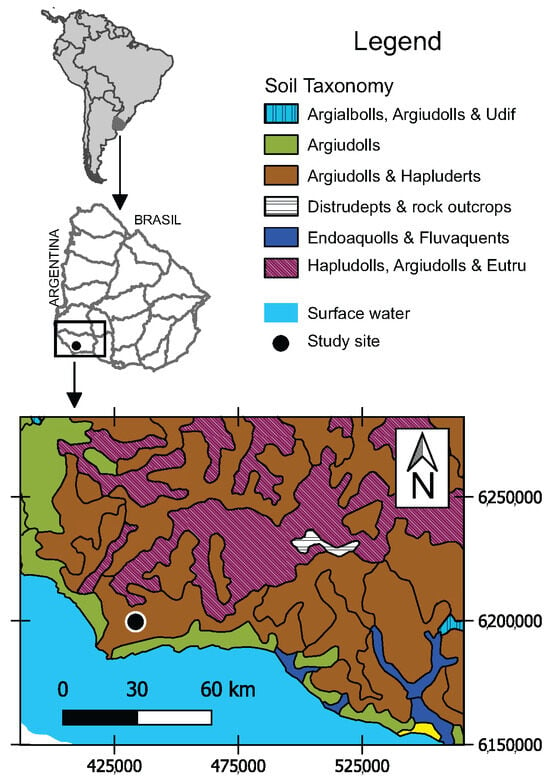
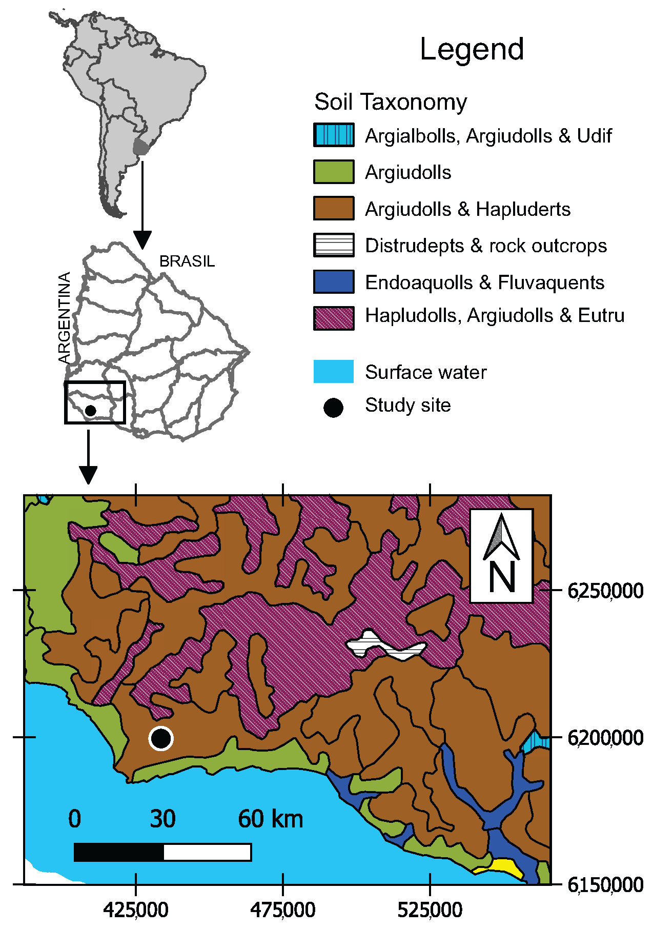
Key resources for assessing the effects of different agricultural systems are long-term experiments (LTEs). Numerous LTEs in the world provide invaluable data on soil health, crop yields, and the environmental impacts of various agricultural techniques. One of the oldest LTEs in South America is located in La Estanzuela, an experimental station operated by the National Institute for Agricultural Research (INIA) of Uruguay. Figure 1 shows the location of the LTE on the soil recognition map of Uruguay. This LTE is located in a soil association dominated by Argiudolls and Hapluderts. These soils are characterized by dark, organic-rich surface horizons and nutrient-rich conditions with medium-to-high fertility, sustaining intensive cropping systems [11,12]. According to [13], this association is the largest in Uruguay, covering approximately 24.9% of the national territory. More than 20% of the Pampas region in Argentina is also covered by this soil [11,14,15]. The Estanzuela LTE has produced significant results during its more than 60 years of development. It features plots with contrasting soil health, including seven different treatments, with three replicates each. This design produced a range of soil conditions, from extreme degradation to very good soil conservation. The plots provide valuable information on the impact of diverse agricultural practices on soil health [16]. These scenarios are likely to reflect the conditions found in different extensive fields across the region, emphasizing the practical relevance of this study.

Figure 1. Uruguay soil recognition map (modified from [17]).

Different studies have warned that soil erosion and degradation represent a threat to global food security and the achievement of the Sustainable Development Goals (e.g., ref. [6]). As such, it is imperative to continue developing new methodologies that contribute to the diagnosis and prevention of soil degradation, as well as to improve the existing ones. Several techniques are used to determine soil structure changes effectively. For example, soil loss can be measured directly, either using barriers in the plots or not. Erosion pins, which are metal rods inserted into the soil, help track changes in the soil surface level over time. Sediment traps are devices placed in runoff pathways to collect eroded soil. According to [18], conventional methods for estimating variations in soil properties are destructive, time-consuming, costly, and do not allow estimation of variability. A possible alternative is, for example, photogrammetry, which involves employing aerial photographs and Geographic Information Systems (GISs) to measure changes in the land surface [19]. Another possibility is to use sensing, based on satellite imagery and drones, to track soil surface changes within large areas [20]. Processing satellite images makes it possible to identify areas with higher vegetation density, which often coincide with areas with soil water accumulation [21]. Although these approaches provide very valuable information on land cover dynamics, they do not allow for precise mapping of the soil horizons, and are conditioned by visibility. Recently, ref. [22,23] showed a method for studying soil erosion caused by rainfall using the Cesium-137 (137Cs) technique, which effectively estimated erosion and the accumulation rates. High-resolution soil mapping in precision agriculture is, in general, costly, primarily because it demands a dense network of sampling points to ensure accuracy [24].

Near-surface geophysics is concerned with the characterization of the shallow subsurface, typically within the first few meters. It employs different physical methods, such as electrical resistivity (ER), induced polarization (IP), electromagnetic induction (EMI), ground-penetrating radar (GPR) and gravimetry, to determine properties such as electrical resistivity, magnetic susceptibility, dielectric permittivity, and mass, which can be related to variables of agronomic and conservation importance, including the soil A horizon thickness (SAHT) [15,25,26,27,28,29,30,31,32]. The advantages of these methods lie in the fact that they allow data to be acquired from the surface of the ground, with minimal or no disturbance to the soil. In addition, measurements can be obtained almost continuously along lines of prospecting. In particular, the ER tomography (ERT) and frequency-domain EMI methods can provide accurate and detailed 2D and 3D images of the electrical resistivity of the soil, with minimal labor and cost [18,28]. Ref. [33] argued that measuring and understanding geophysical properties can be significantly beneficial for agriculture and environmental impact analysis.

Advances in CPUs and electronics in recent decades have enabled the development of different ER acquisition systems focused on surveying large portions of soil and processing the data in short times. In particular, Veris (Veris Technologies Inc., Salina, KS, USA, [34]), ARP (Geocarta, París, France, [35]), and RMCA-3 (Société SEPTA, Roquefort-la-Bédoule, France, [36]) are examples of Wenner based electrode–soil contact systems used to acquire and process electrical resistivity data in real-time [26,31,37,38]. These advances are motivated by the relevance of obtaining high-resolution 2D and 3D ER images of the soil [39], which are useful, particularly, in agricultural research (e.g., ref. [40,41,42]). Improvements in these subjects are challenging due to the need to position electrodes accurately, and allow for a variety of electrode arrangements. Additionally, the energy requirements to carry out these processes must be compatible with the characteristics of a portable source (e.g., ref. [43]). Current EMI systems, on the other hand, can be a useful complement to ER systems, mainly due to their capabilities to rapidly acquire data and produce 2D horizontal electrical images of the subsurface [30,32,44].

In South America, ERT and EMI have been applied individually in agricultural studies to investigate different characteristics and processes occurring in the vadose zone (e.g., refs. [45,46,47,48]). However, the use and benefits of using these methods together in agronomy have not been addressed to date in the region. The combined use of ERT and EMI leverages the complementary advantages of both methods [49,50]. EMI allows for rapid and cost-effective mapping of surface and near-surface variability [32,51]. ERT, on the other hand, provides a proven capability to define strata [52,53], albeit at a higher operating cost and with less spatial coverage than EMI. Integrating both techniques reduces the ambiguities associated with EMI alone, while optimizing the cost-depth ratio compared to surveys based solely on ERT [54]. This complementary framework is particularly relevant for agronomic applications in South America, where high-resolution soil information is needed over large areas, but budgetary and operational constraints, along with equipment availability, often limit the use of geophysical methods. This study evaluates a combined methodology of ERT and EMI, as well as core sampling, to characterize and interpret the soil of La Estanzuela LTE, and, centrally, to map its SAHT, under various agronomic treatments. To reduce the installation time of ERT surveys and reduce human effort, a mounting electrode system was designed and implemented. The soil considered, a smectitic Vertic Argiudol with a silty clay loam texture, refs. [17,55] is of relevance, since it is one of the most productive in Uruguay and the region. The evaluated methodology focused on producing quick but sufficiently accurate SAHT maps for fields or plots of commercial agriculture. The overarching objective is to demonstrate the potential of this type of approach to improve soil characterization and generate actionable data for sustainable land management under varied treatment conditions.

2. Materials and Methods

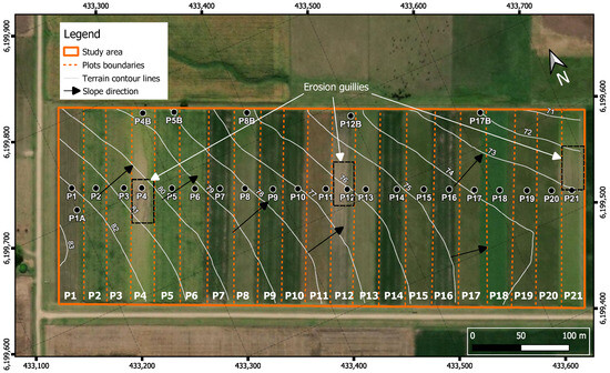
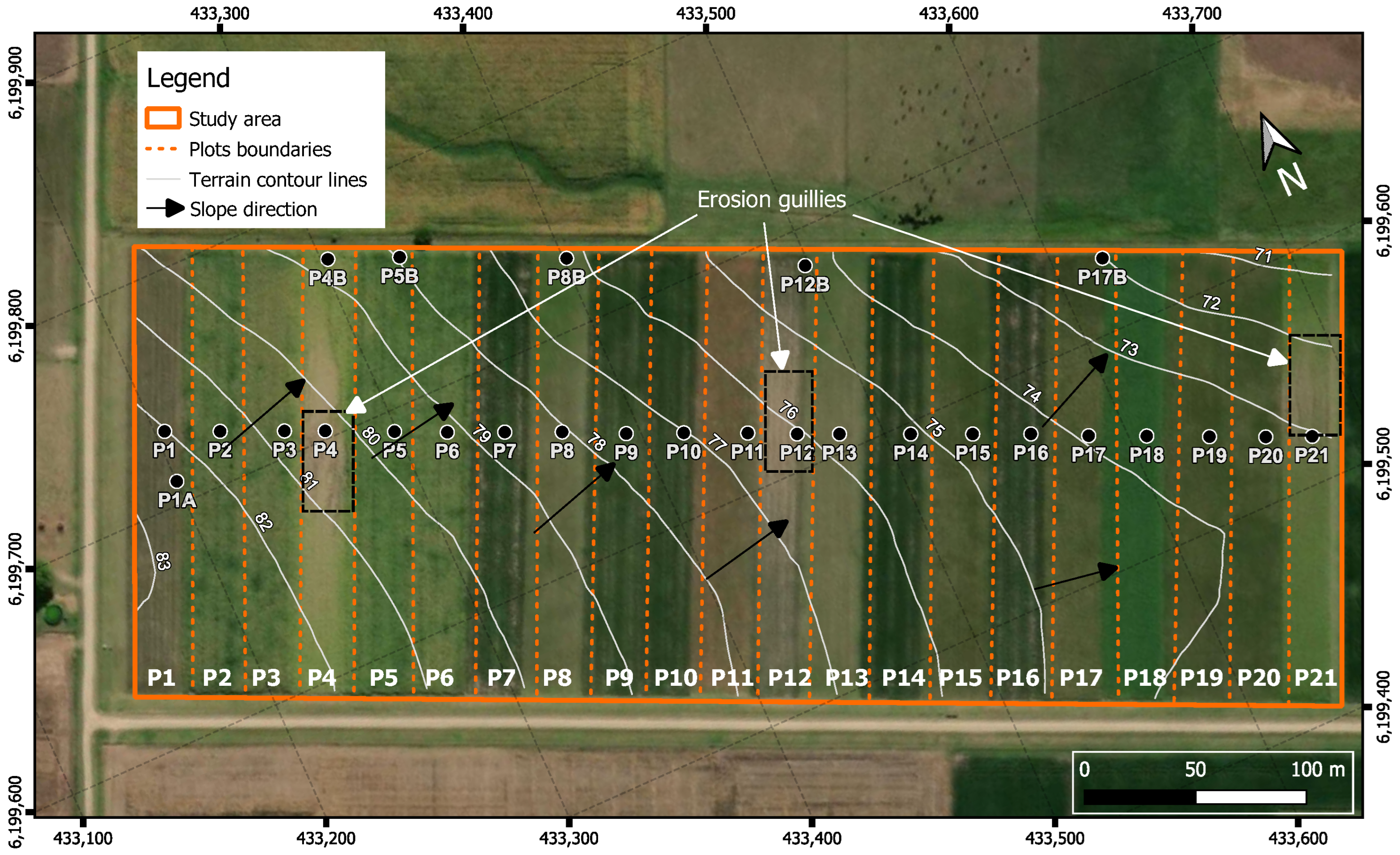
In 1963, an experiment started at the La Estanzuela experimental station to demonstrate the critical importance of crop and pasture rotation for preserving and improving soil productivity [56]. The main objective of this LTE was to study the effects of different crop and crop–pasture rotations, each with several replicates, on soil quality, crop yield, and environmental impact [57]. The experiment analyzed here consists of 21 plots, each 25 m wide and 200 m long, with no animal grazing. Figure 2 shows the LTE with topographic contour lines at 1 m intervals obtained from the Digital Elevation Model (DEM) provided by the Spatial Data Infrastructure of Uruguay [58].

Figure 2. Crop–pasture rotation experiment plots at La Estanzuela. The study area (orange) includes 21 plots (P1–P21), with contour lines (1 m intervals), slope direction, and gully erosion features are indicated (black dashed boxes).

The DEM has a spatial resolution of 2.5 m per pixel, providing a sufficiently detailed representation of the terrain. The slope direction (black arrows) is, on average, oriented toward the northeast. This direction agrees with the location of the FOS, where sedimentation is expected to occur. Comprehensive data on the plots of Figure 2 have been obtained over time, including crop yields, soil properties, erosion rates, water quality, and economic performance [56]. Contrasting treatments of the plots have allowed the observation of appreciable differences in soil degradation and fertility, information that significantly contributed to the development of sustainable agricultural practices [16,56,59,60]. The actual soil management scheme is shown in Table 1.

Table 1. Schematic summary of the seven continuous cropping (CA) or crop–pasture rotation (CPR) treatments studied in the rotation experiment at La Estanzuela.

System	Plots	Fertilizer	Acronym
S1	P4, P12, P21	without	CA
		fertilizer
S2	P5, P9, P18	+P	CAF
		+N
S3	P2, P11, P19	+P	${\mathrm{CPR}}_{50}$
		+N
S4	P3, P13, P15	+P	${\mathrm{CPR}}_{66}$
		+N
S5	P6, P8, P20	+P	${\mathrm{CPR}}_{50}$
		+N
S6	P7, P10, P16	+P	CAF
		+N
S7	P1, P14, P17	+P	${\mathrm{CPR}}_{33}$
		+N

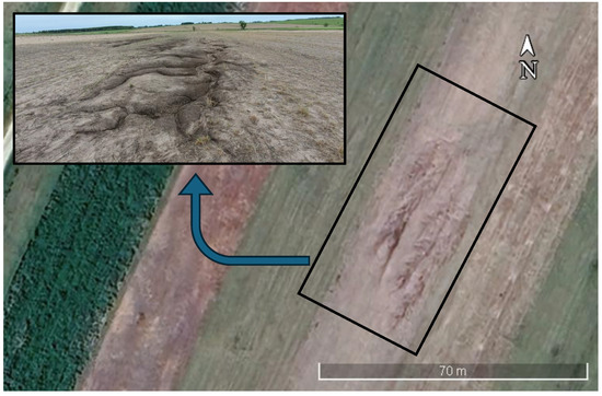
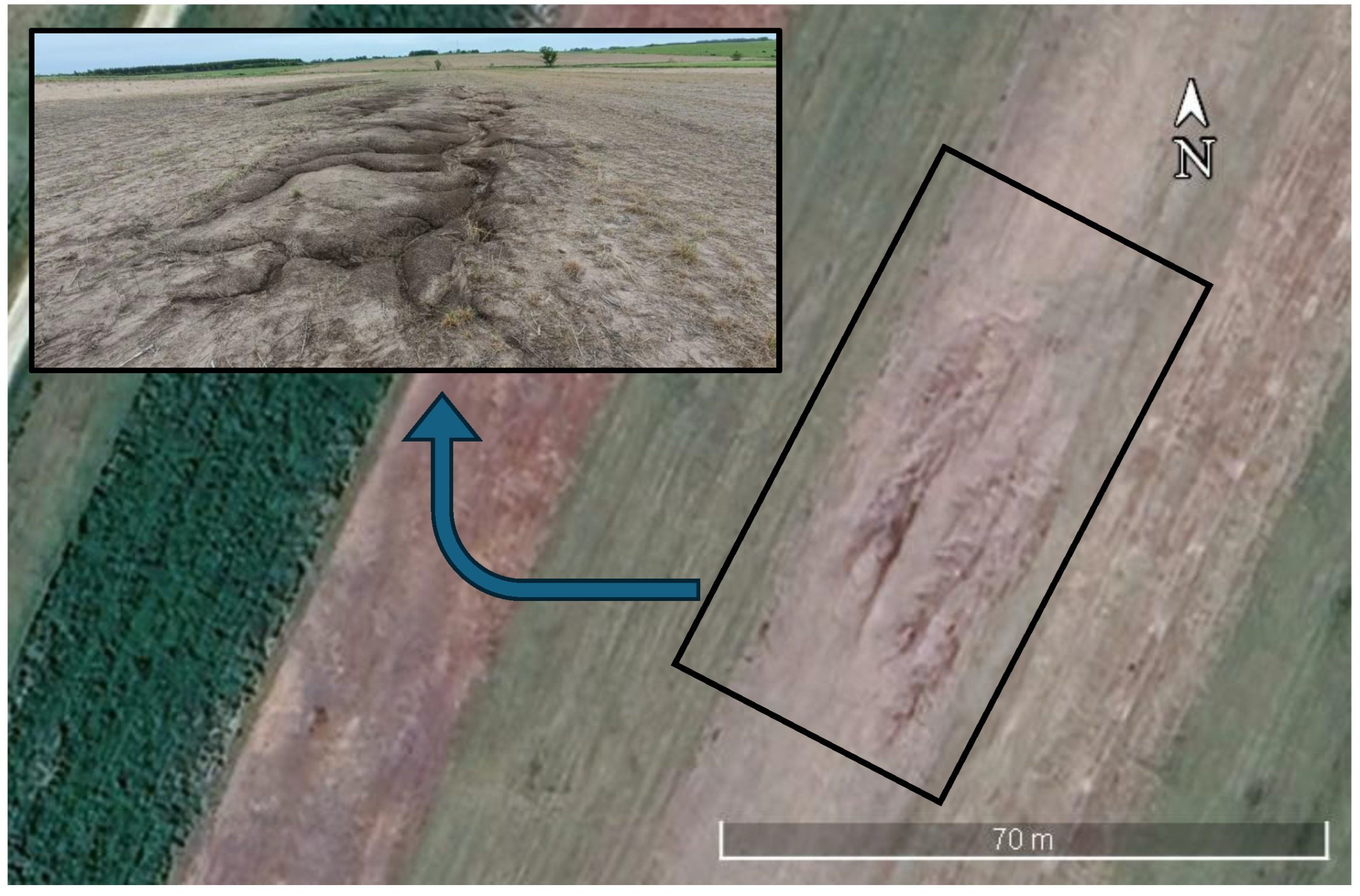
S1 is a continuous cropping system without fertilizers added (CA). S2 and S6 are continuous cropping systems with fertilizers added (CAF). The other four systems are fertilized and have crop–pasture rotations (CPRs) with 33% (${\mathrm{CPR}}_{33}$), 50% (${\mathrm{CPR}}_{50}$) and 66% (${\mathrm{CPR}}_{66}$) pasture proportions and different species compositions. According to [59], CPRs resulted in higher concentrations of soil organic carbon (SOC) and total nitrogen (Ntot). Ref. [60] showed that CPRs were effective in reducing the negative effects of continuous annual agriculture systems on soil quality and corn yields. In the center of plots P4, P12, and P21, which received treatment CA (Figure 2 and Table 1), dendritic gullies, one of the most intense types of erosion created by water flow [61], can be observed (Figure 3).

Figure 3. Satellite view with surface photo of the active gully of P4, showing erosion features within the experimental area.

These gullies, which erode the soil and deplete the fertile A horizon, resemble a branching three pattern, formed by the convergence of smaller channels into larger ones [7]. Based on the topographical characteristics of the site (Figure 2), eroded sediments have probably been deposited at the FOS.

The dominant soils in La Estanzuela are Mollisols, specifically smectitic Vertic Argiudolls (Figure 1), according to the USDA Soil Taxonomy [16,17]. These soils are dark, characterized by a silt clay loam texture (29.2% clay on average), naturally fertile and moderately well drained, located on gentle hills with a slope of 2% to 4%. They are developed on silty clayey sediments of the Quaternary-aged Libertad Formation [62]. The Libertad Formation (Lower Pleistocene) consists of mudstones, loess, and mudrocks with variable percentages of sand and clay, brown to reddish brown in color, indicating continental peridesert sedimentation [63]. According to [64], the content of silt and clay varies between 85% and 100%, with the clay fraction predominantly composed of calcium smectite, secondary illite, and occasional kaolinite. This type of formation is characterized by low hydraulic conductivity [65], which restricts groundwater flow [66].

2.1. Geophysical Methods

2.1.1. Background of the Applied Geophysical Methods in the Study Area

The effectiveness of ERT in characterizing tilled soil layers has been highlighted, for example, in [27]. This study demonstrated how ERT could be used to accurately map subsurface features and monitor changes over time. In Uruguay, a comprehensive ERT study of the Libertad Formation was performed by [47], obtaining electrical resistivity values between 5 and 17 $\Omega$m. Comparable electrical resistivity values were reported for this formation by [67] in La Estanzuela, showing the consistency of the measurements across different locations. However, no other studies of the electrical resistivity characteristics of the Libertad Formation, either with ER, EMI or other methods, have been published.

2.1.2. EMI Survey

The EMI method is based on the measurement of the change in the self impedance of a coil or mutual impedance between coils due to the presence of the soil and soil variations, specifically in its electrical conductivity and magnetic susceptibility [68]. In other words, EMI instruments generate an alternating magnetic field that induces small currents in the ground. These currents create a secondary magnetic field that is measured by the system. For low induction numbers, the ratio of the quadrature component of the secondary magnetic field to the primary magnetic field is approximately proportional to the soil apparent electrical conductivity [69], as expressed in the following formula (Equation (1)):

$${\sigma }_a\approx {\displaystyle \frac{4}{\omega {\mu }_0{s}^2}}\left({\displaystyle \frac{H_s}{H_p}}\right)$$

(1)

where

• ${\sigma }_a$ is the apparent soil conductivity [mS/m];
• $\omega$ is the angular frequency of the electromagnetic field being used;
• ${\mu }_0$ is the permeability of free space;
• s is the separation distance between coils (two-coil system);
• $H_s$ is the quadrature component of the secondary magnetic field;
• $H_p$ is the primary magnetic field.

This expression makes it possible to directly calculate the electrical conductivity from the measured fields and the setup of the system.

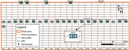
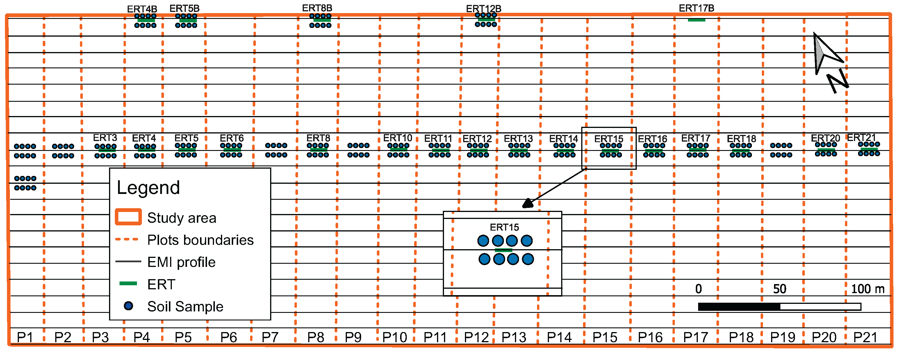
The EMI data were acquired using a two-coil frequency domain EM38 system (GEONICS, Mississauga, ON, Canada). This instrument is often used in agriculture applications (e.g., ref. [70]) and other areas of investigation due to its light weight and small size, in addition to reliability [31]. It operates at a frequency 14.5 kHz, with a selectable inter-coil spacing of 0.5 or 1 m. The coils were oriented vertically coplanar (VCP), as this results in greater sensitivity to shallow soil depths [51,69] with an approximate investigation depth of 0.75 m [71], sufficient for the purposes of this study. Parallel survey lines were deployed across the experimental area, in an approximate SE-NW direction, with a total of 21 parallel lines spaced 10 m apart. Figure 4 shows a diagram of the experiment, including the 21 plots, the transects surveyed using the EMI and ERT methods, and the coring sites.

Figure 4. Layout of geophysical surveys and soil sampling sites across the experimental plots. EMI profiles (black lines), ERT locations (green bars), and soil cores (blue circles) are shown within the study area.

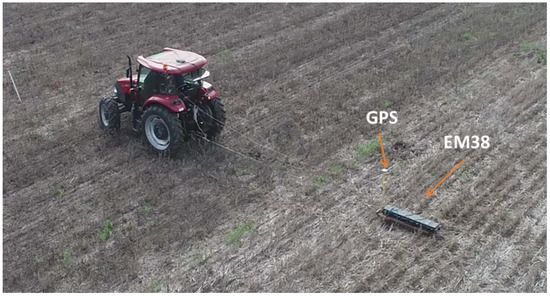
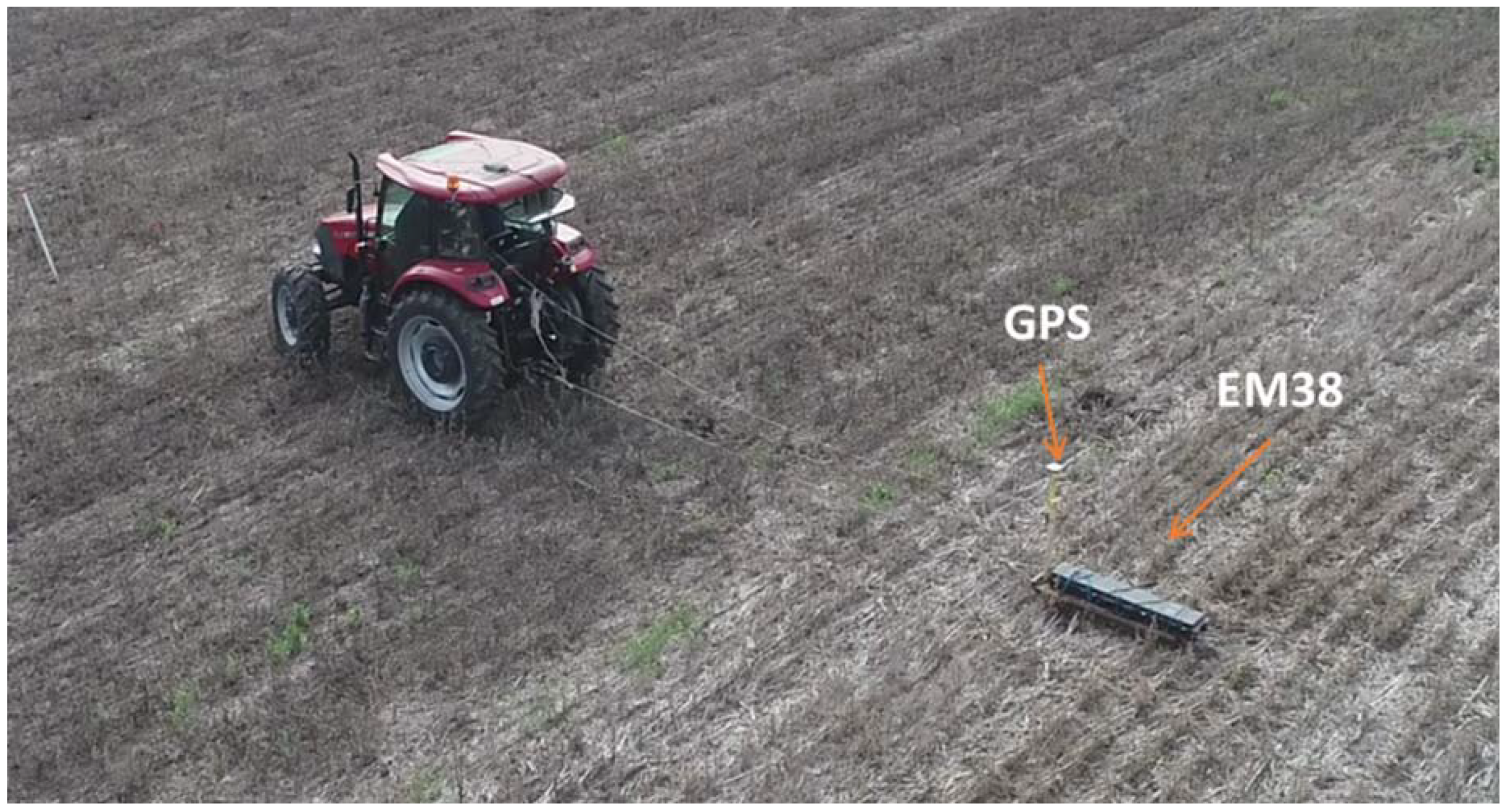
The EMI unit was mounted in a shockproof case tied to a homemade sled, constructed from glued wooden parts. A GPS-guided tractor was used for towing the EMI unit (Figure 5).

Figure 5. EM38 induction equipment mounted on a wooden sled and driven by a GPS-controlled tractor.

Positions were georeferenced using a Geode differential GPS (Juniper Systems). The coil orientation was vertical (horizontal dipoles), in order to minimize the effective depth range of the measurements, and data were acquired at a rate of 1 ${\mathrm{s}}^{-1}$, with a mean travel speed of 1 m/s along the survey lines. The survey covered an approximate area of 0.1 km² and took 1.25 h. The temperature correction was deemed unnecessary, as the mean soil temperature was $24.81°\mathrm{C}$ with a standard deviation less than $3.8°\mathrm{C}$, indicating very low variability.

2.1.3. ERT Survey

The ER method is based on injecting a DC electrical current into the soil through a pair of electrodes and measuring the resulting voltage difference between another pair of them. In ERT, several combinations of injection and measurement pairs are used around each position of the survey line in order to electrically map the soil below, not only horizontally but also in depth. Each current–voltage difference data pair determines an apparent resistivity value as follows:

$${\rho }_a=K\left({\displaystyle \frac{\Delta V}{I}}\right)$$

(2)

where

• ${\rho }_a$ is the apparent soil resistivity [$\Omega$m];
• $\Delta V$ is the voltage difference [V];
• I is the injected current [A];
• K is a factor that depends on the geometry of the injection and measuring electrodes being used [m].

Once the apparent resistivity of all electrode combinations that are part of the measurement design is obtained, an electrical resistivity profile can be calculated by inverting the data.

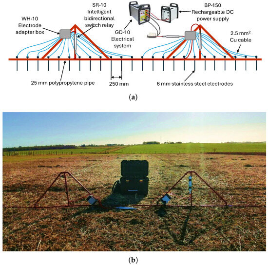
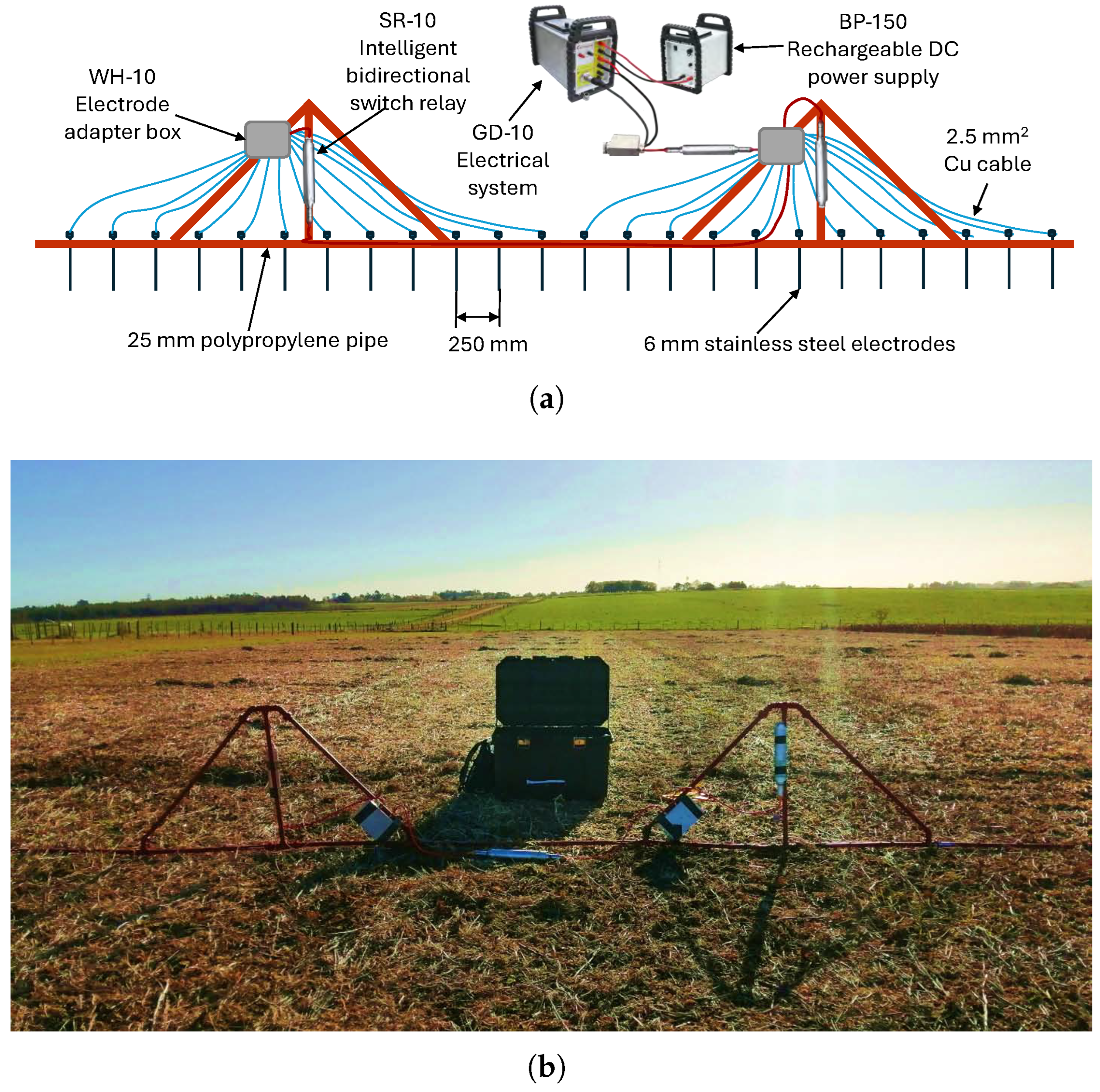
A novel electrode mounting system was designed and constructed to reduce installation time and simplify and speed up the positioning and insertion of the electrodes into the soil, as well as wiring between the electrodes and the resistivity meter, a GD-10 (GEOMATIVE, Shenzhen, China) unit. The mounting system was built with 25 mm diameter polypropylene tubes and fittings to provide rigidity and prevent electrical contact between the electrodes (Figure 6a). Figure 6b shows the electrode mounting system during measurement.

Figure 6. (a) Scheme of the electrode mounting system. (b) Electrode mounting system.

The system has a maximum of 24 injection/voltage electrodes spaced $a=250\mathrm{mm}$ apart, resulting in a total survey line length of 5.75 m. For this setup, the theoretical depth of exploration is approximately one meter, sufficient for the objectives of the survey. The electrodes were manufactured from M6 stainless steel threaded rods, with a diameter of $\varphi =6\mathrm{mm}$ and a length of 100 mm. The ratio $a/\varphi$ is approximately 42, which is consistent with the recommendation of [72] to be greater than 31.5. Electrodes were wired using copper conductors to a connection box provided by the manufacturer of the resistivity meter. A total of 20 Electrical Resistivity Tomography (ERT) surveys were conducted in La Estanzuela. These survey lines crossed the plots parallel to the EMI lines (Figure 4). Most of the lines were located in the central part of the plots (P1–P21),where relatively low values in EMI resistivity and high variability were observed, while others were placed near the northeastern end (P4B, P5B, P8B, P12B, and P17B), close to the FOS, in which the highest values of EMI resistivity were observed. A Wenner–Schlumberger configuration was utilized to acquire the data. The number of electrodes was the maximum allowed by the electrode mounting system. The average time required to position the electrode mounting system and acquire the data was 5–7 min per survey line, which implied a 60% decrease with respect to the alternative of handling the electrodes and wires individually, as well as a significant reduction in human effort. Data were processed and inverted with RES2DINV v4.0 (GEOTOMO, Gelugor, Malaysia; [73]).

2.1.4. Soil Coring

Soil coring was performed along the ER survey lines, at the points indicated in Figure 4. The sampling was carried out using a hydraulic corer mounted on the three-point hitch of a tractor. Eight cores, each up to a depth of 0.9 m, were extracted per ER survey line. Once the tube reached the maximum depth, the corer was carefully lifted to ensure that the soil sample remained intact within the tube. Each core was then removed from the corer tube and placed together with the other cores for direct inspection. Different layers were identified from the color, texture, and apparent organic matter content of the samples. These were interpreted on the basis of the pre-existing knowledge of layers A–C [13,74]. The correspondence between observations and available information was high, ensuring the reliability of the interpretation. The average position of each horizon contact was marked on the core samples and photographed. The average thicknesses of the A and B soil horizons were recorded. The core samples were sectioned and prepared for transport to the laboratory for texture analysis.

3. Results and Discussion

3.1. EMI Electrical Resistivity Map

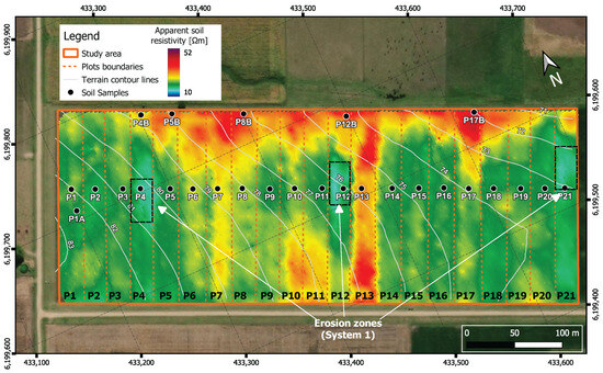
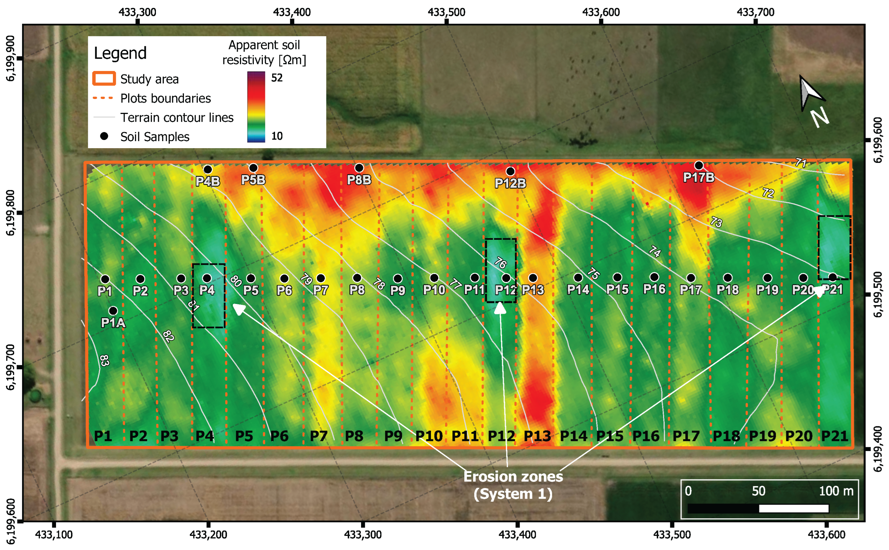
An electrical resistivity map was generated by applying geostatistical analysis to the electrical conductivity data obtained through EMI. Ordinary Kriging interpolation was used to estimate spatial variability and produce a continuous electrical conductivity surface across the experimental plots. An exponential variogram model was fitted with a range of 90, a nugget of 1, and a sill of 70. Interpolation was performed with a search radius of 20 and 64 neighbors. Cross-validation yielded a mean error of −0.085 mS/m and RMSE of 0.397 mS/m. The interpolation results, converted into electrical resistivity values, are shown in Figure 7. The map was used to analyze the spatial distribution of soil bulk electrical resistivity.

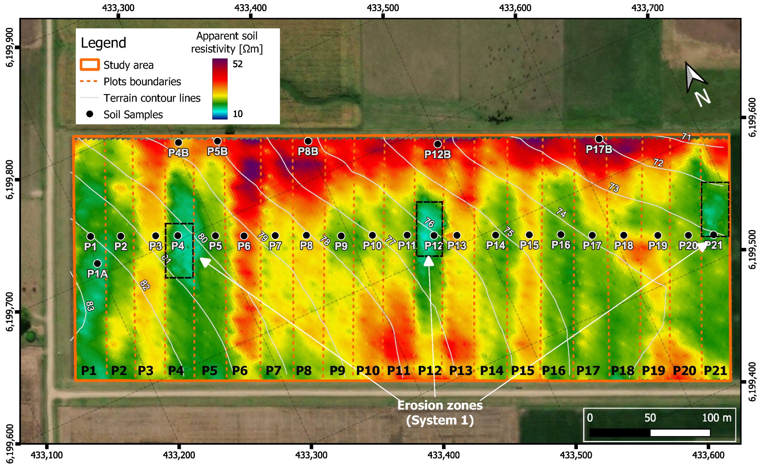
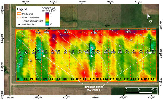
Figure 7. Soil electrical resistivity map of the study area. Plot boundaries, soil sample sites, and erosion zones indicated are shown (black dashed boxes).

Bands of relatively high and low electrical resistivity are observed, which roughly coincide with the arrangement of the plots. Variability of this property is also observed within the plots. It is noteworthy that the eroded spots visible in Figure 2 (P4, P12 and P21) coincide with areas of Figure 7 with low electrical resistivity values. In contrast, the most preserved plots (i.e., P3, P6, P13, P15), on average, exhibit relatively large resistivities. The maximum of electrical resistivity occurs at the lowest parts of the experiment, where eroded sediments are likely to accumulate.

3.2. ERT Profiles and Soil Coring

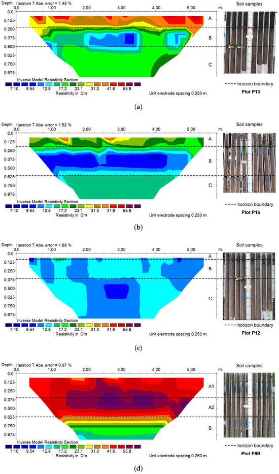
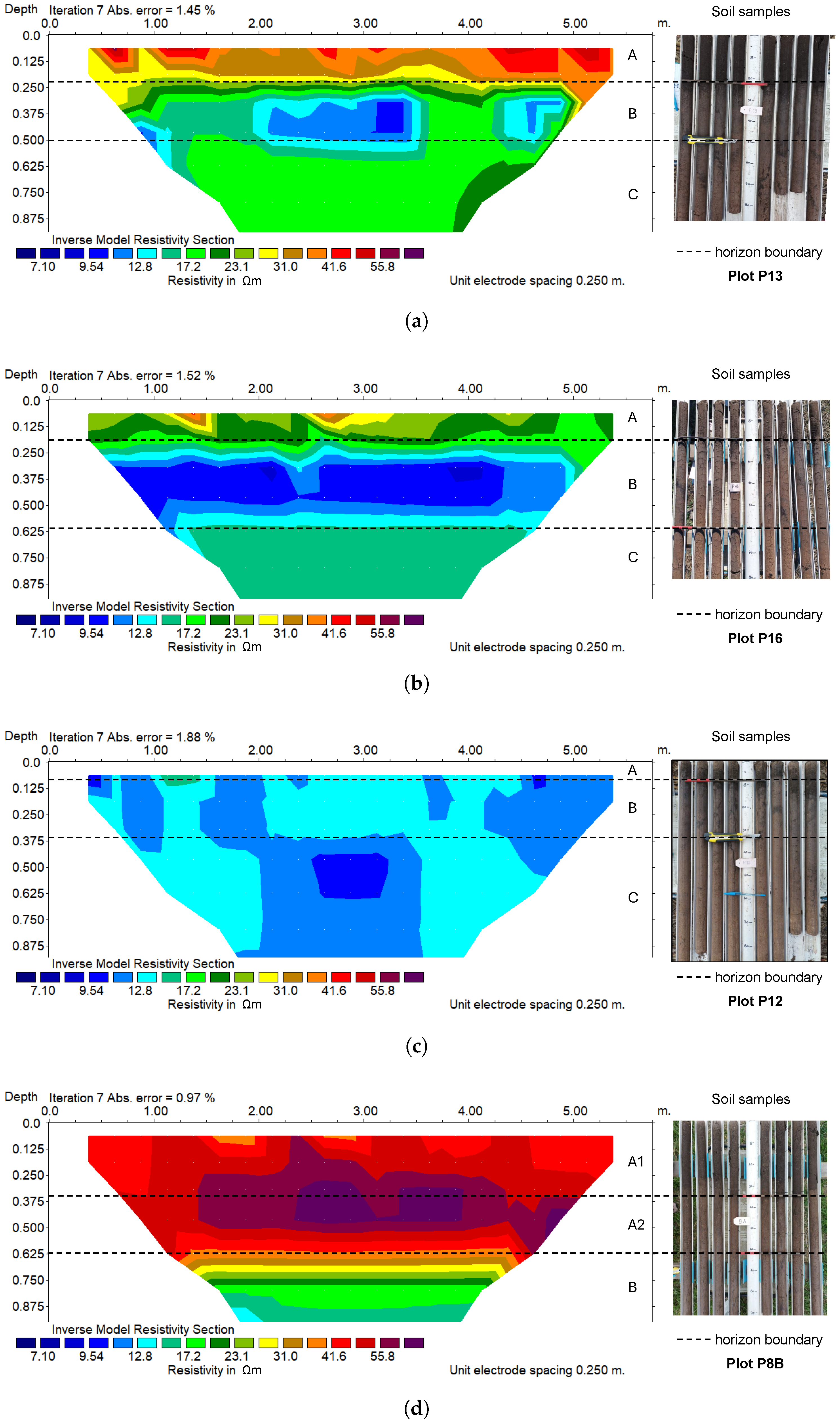
The ERT data were inverted and plotted using a common color scale and a linear depth scale. Figure 8 shows examples of each type of behavior identified in the ERTs, corresponding to ERT13, ERT16, ERT12, and ERT8B, together with matching photographs of the extracted soil cores. The remaining ERT images can be found in the Supplementary Materials. The dashed lines mark the bottom of the A and B horizons, as determined from the direct inspection of the core samples. They were used as a reference in the interpretation of the ERT images. In Figure 8a, Figure 8b and Figure 8d (${\mathrm{CPR}}_{66\%}$, CAF and FOS, respectively), layers with different electrical resistivity values can be distinguished. The base of shallowest layer, which is also the most contrasting interface between layers, coincides with the position of the A–B contact obtained from the soil cores. Figure 8d shows a relatively thick two-layered A horizon, illustrating sediment deposition in the FOS zone. In Figure 8c, the A–B electrical transition cannot be clearly distinguished, since it almost coincides with the upper limit of the image. The contacts between B and C horizons are observed in Figure 8a–c, with varying clarity and contrast. In Figure 8a,b, the electrical resistivity values of C are intermediate between those of A and B, while in Figure 8c, the electrical resistivity values of B and C are quite similar.

Figure 8. ERT profiles alongside extracted soil cores: (a) ERT13, (b) ERT16, (c) ERT12 and (d) ERT8B. The dashed line marks the bottom of the A and B horizons as deduced from the soil samples. Letters A, B, C, A1, and A2 denote soil horizons and subhorizons.

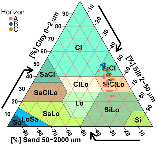
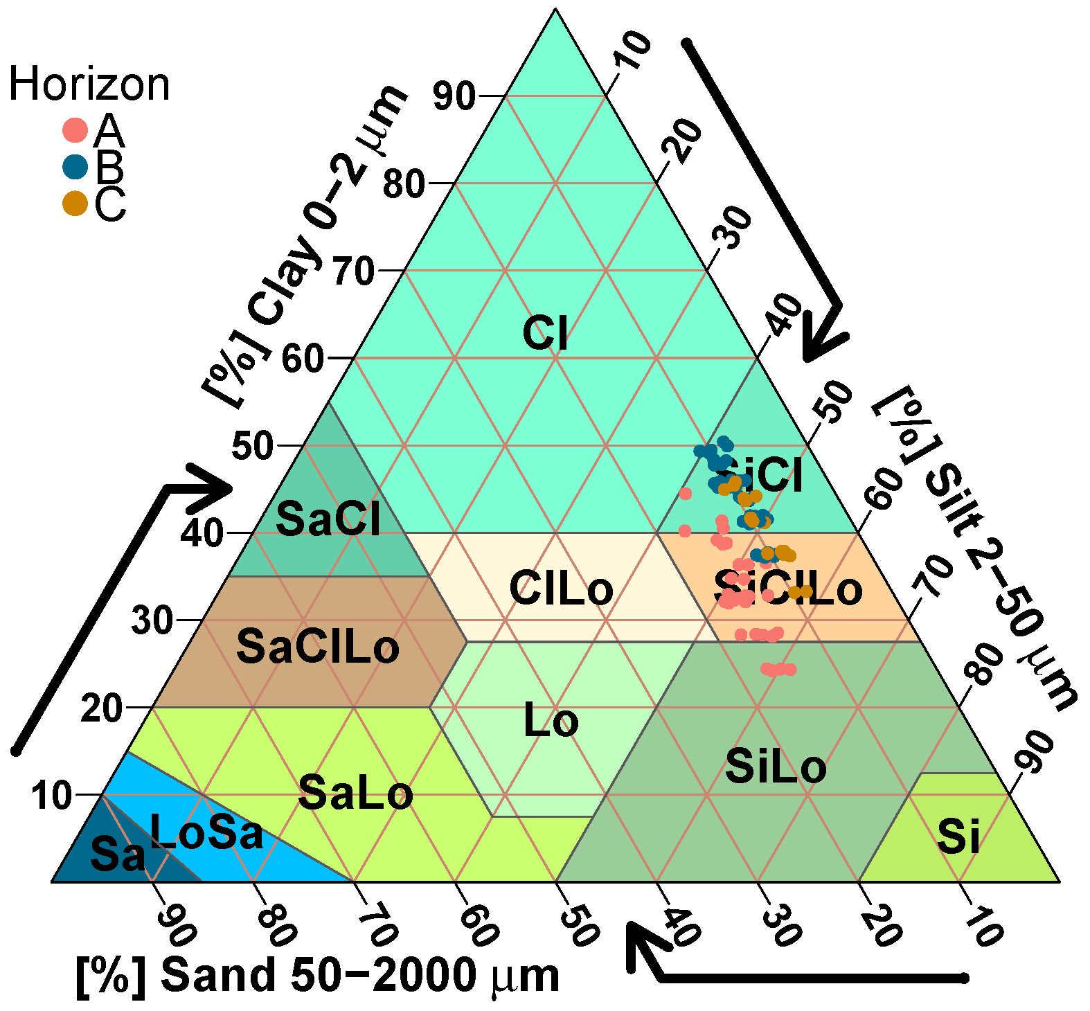
The A–B and B–C contact positions deduced from Figure 8 were verified by comparing the textures of resulting horizons, in order to determine if they are truly different and in accordance with the information available in the literature [75,76]. To do this, textures from the extracted soil cores, which were originally sectioned according to the depth intervals 0–0.1 m, 0.1–0.2 m, 0.2–0.4, 0.4–0.6 m and 0.6–0.8 m, were measured [77]. The percentages of sand, silt and clay obtained for these intervals were then averaged vertically by weighting them with the proportion of assumed A, B and C intervals with which each textural interval coincides. These results were finally averaged along the survey direction and plotted in a textural triangle (Figure 9) by using the Soiltexture v1.5.3 software package [78]. The result of Figure 9 shows grouping of the texture data by horizon, with groups clearly differing in their sand content. For the A horizon, the average sand content is approximately 15%, while for B and C horizons, the average sand content is around 10%.

Figure 9. Soil texture triangle showing the classification of Horizons A, B, and C based on sand, silt, and clay content.

The acronyms used in the textural triangle are explained in Table 2.

Table 2. Soil types (modified from [79]).

N	Acronym	Type
1	Cl	clay
2	SiCl	silty clay
3	SaCl	sandy clay
4	ClLo	clay loam
5	SiClLo	silty clay loam
6	SaClLo	sandy clay loam
7	Lo	loam
8	SiLo	silty loam
9	SaLo	sandy loam
10	Si	silt
11	LoSa	loamy sand
12	Sa	sand

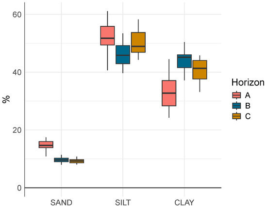
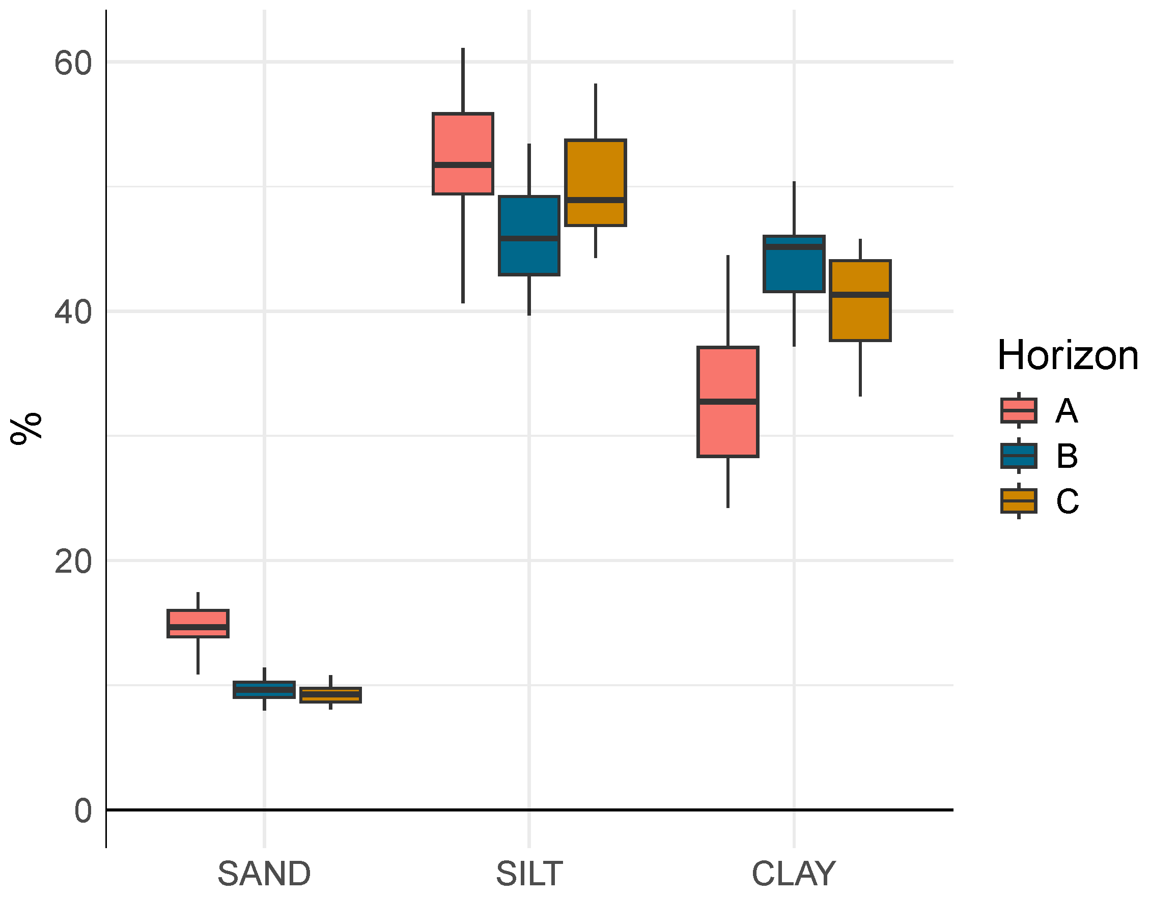
In Figure 10, the textural data of Figure 9 are represented in box plots for each textural category: sand, silt and clay.

Figure 10. Boxplot of sand, silt, and clay percentages in soil A, B and C horizons.

Pairwise comparisons between soil horizons (categories A, B, and C) were conducted using the Wilcoxon rank-sum test to assess differences in soil texture variables. The results are shown in Table 3.

Table 3. Pairwise Wilcoxon test results for soil texture horizons.

Variable	Horizons	${\mathrm{n}}_1$ vs. ${\mathrm{n}}_2$	Adjusted p-Value	Significance
	A–B	32 vs. 45	$4.56\times {10}^{-13}$	****
SAND	A–C	32 vs. 19	$1.01\times {10}^{-8}$	****
	B–C	45 vs. 19	0.339	ns
	A–B	32 vs. 45	$4.5\times {10}^{-6}$	****
SILT	A–C	32 vs. 19	0.57	ns
	B–C	45 vs. 19	0.006	**
	A–B	32 vs. 45	$7.56\times {10}^{-11}$	****
CLAY	A–C	32 vs. 19	$5.22\times {10}^{-5}$	****
	B–C	45 vs. 19	0.014	*

where *, **, and **** indicate statistical significance (p < 0.05, p < 0.01, and p < 0.0001, respectively), while ns denotes non-significant differences.

The analysis of sand content in the soil horizons shows that the A horizon differs significantly from both the B and C horizons (adjusted p-values = $4.56\times {10}^{-13}$ and $1.01\times {10}^{-8}$, respectively), while the B and C horizons do not show a significant difference. For silt content, significant differences were observed between the A and B horizons (p = $4.5\times {10}^{-6}$) and between B and C (adjusted p = 0.006), whereas A and C horizons did not differ significantly (adjusted p = 0.57). Clay content varied significantly across all horizons. The A horizon differed strongly from both B and C (adjusted p-values = $7.56\times {10}^{-11}$ and $5.22\times {10}^{-5}$, respectively), and a moderate but significant difference was also found between the B and C horizons (adjusted p = 0.014). This reflects a progressive change in clay accumulation with depth. These characteristics are consistent with those informed in the literature for the site [75,76]. In general, sandy media are characterized by higher electrical resistivity than silty media, and silty media, in turn, by higher resistivity than clayey media. Therefore, the resistivity differences observed in ERT profiles between A and B–C are likely due to the higher sand content in A, while the smaller differences between B and C are probably produced by the slightly lower clay content in the latter [80]. Considering the textural results obtained for the A, B and C horizons, this seems to be a feasible explanation of the type of electrical response observed in the ERT profiles. While confounding factors could potentially affect the relationship between soil resistivity and texture, these were minimized by conducting the study under stable moisture conditions and in an area with limited microtopographic variability. Although discrete, the soil cores were strategically placed to intersect the main resistivity contrasts (Figure 4), ensuring that the sampled horizons were representative of the units interpreted along the transect. The shallow depth investigated (<1 m) and the clear stratification observed in the field further reduced the likelihood of abrupt lateral variations not captured by the cores. While additional tests, such as supplemental boreholes, in situ moisture measurements, or laboratory conductivity analysis, could refine the horizon characterization, the combined evidence from the ERT data, field observations, and particle size analyses was sufficient to support the presented textural interpretation.

3.3. Electrical Characterization of Soil Horizons

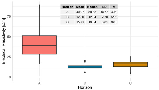
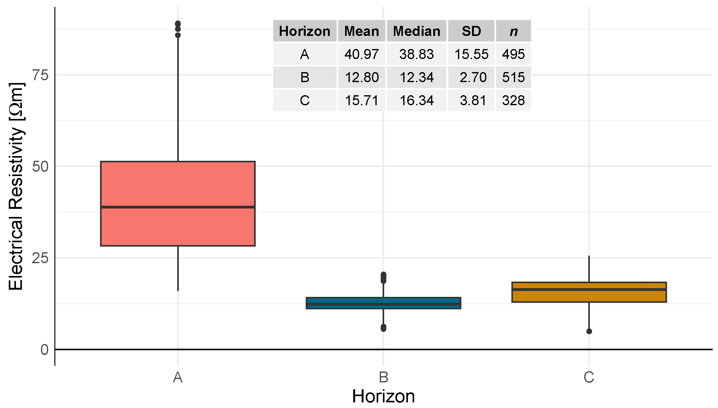
To verify the electrical resistivity interpretation of the soil of La Estanzuela, a characterization of the A, B, and C horizons was performed by analyzing the ERT values above and below the corresponding contact position. For each horizon, n = 495, n = 515 and n = 328 electrical resistivity values were considered, respectively. The main statistics of these data sets are represented in the box plot in Figure 11 and in the inserted table. These results indicate that different resistivity distributions very likely characterize layers A, B and C.

Figure 11. Boxplot illustrating the electrical resistivity statistics for soil A, B and C horizons.

Pairwise comparisons between the A, B and C horizons using the Wilcoxon rank-sum test (Mann–Whitney U) revealed statistically significant differences in resistivity distributions. In all cases, the p-value was less than $2.2\times {10}^{-16}$, indicating that the observed differences in central tendency are highly unlikely to be due to random variation. These results confirm that each horizon represents a distinct population in terms of electrical resistivity. This indicates that the resistivity obtained through ERT can be used as a valid criterion to differentiate the A, B and C horizons in this agronomic experiment. The subsurface exhibits a three-layer behavior down to a depth of approximately 1 m, with an electrical resistivity that decreased from the upper layer to the underlying one, and increased slightly in the third layer. Considering the SAHT and SBHT observed in the ERT profiles, and the typical investigation depth of the EMI instrument for the employed dipole configuration, the EMI in this experiment reflects the lateral variability of a band of approximately constant thickness that includes the first layer and most of the second, as further discussed in Section 3.4. Under this model, when the upper layer is thinner, the instrument captures a stronger signal from the underlying horizon, and the overall electrical resistivity decreases, and vice versa, as observed in the degraded and preserved plots, respectively, as well as the anomalous areas within the plots. As a consequence, the ERT and EMI results complementarily allow for the vertical and horizontal characterization of A horizon, including the interpretation of the horizons boundaries and different heterogeneities.

3.4. Linear Regression Models (LRMs) for Estimating SAHT

The depth of investigation (DOI) in EMI measurements is commonly defined as the depth range where up to 70% of the cumulative sensitivity response function occurs [69,71]. This depth depends primarily on the coil spacing and orientation. In the vertical coplanar (VCP) mode used, the DOI is approximately 0.75 times the coil spacing; therefore, for a 1 m spacing, the effective depth is approximately 0.75 m. Since the A and B horizons occupy most of this depth range, the EMI signal is mainly sensitive to these two layers. The C horizon lies at or just below the main sensitivity zone and contributes only marginally to the response, especially because it is a few $\Omega$m higher than the B horizon. Therefore, the EMI measurements in La Estanzuela LTE primarily reflect the properties of the A and B horizons, with minimal influence from the C horizon.

Under these circumstances, a simple relationship between EMI electrical resistivity and the A–B transition depth could be expected. This is so as long as the lateral variations in moisture, temperature, and dissolved salts and electrolytes within each layer cause only secondary variations in resistivity [51]. To evaluate the possibility of the existence of a simple mathematical relation between the SAHT and EMI data, the average EMI electrical conductivity and resistivity, along with the soil A horizon thickness obtained from each core sample, were considered (Table 4). The logarithm of the EMI electrical resistivity, which is a variable often used in ERT analysis, and the DEM elevation were also included in the analysis to test whether they allowed for improved results.

Table 4. Data used for obtaining a LRM for estimating SAHT.

ID	RE	CE	Z	SAHT
P1	22.18	45.09	11.04	20
P2	22.15	45.15	10.5	16
P3	26.38	37.91	9.62	20
P4	18.01	55.52	10.22	10
P5	23.71	42.18	8.15	18
P6	36.75	27.21	8.65	23
P7	27.51	36.35	7.66	18
P8	27.7	36.10	7.05	22
P9	22.82	43.82	6.48	21
P10	25.57	39.11	6.05	21
P11	24.28	41.19	5.5	22
P12	18.88	52.97	5.05	8
P13	28.58	34.99	4.75	23
P14	24.8	40.32	4.12	23
P15	27.22	36.74	3.64	24
P16	22.35	44.74	3.24	19
P17	22.87	43.73	2.89	18
P18	27.64	36.18	2.67	25
P19	25.46	39.28	2.51	24
P20	23.67	42.25	2.24	20
P21	20.21	49.48	2.08	9
P1A	18.59	53.79	11.4	12
P4B	27.66	36.15	7.79	38
P8B	42.51	23.52	5.25	62
P12B	47.06	21.25	3.33	60

where ID: identification of sampling points indicated in Figure 7 and Figure 12; RE: apparent EMI electrical resistivity [$\Omega$m]; CE: apparent EMI electrical conductivity [Siemens/m]; Z: elevation with respect to the lowest part of the experiment; and SAHT: soil A horizon thickness [cm].

A Pearson correlation test demonstrated that the EMI electrical resistivity and elevation are independent (r = −0.204; p-value = 0.338), as well as the EMI electrical conductivity and elevation (r = 0.255; p-value = 0.229).

LRMs to predict SAHT were calculated for six models using different combinations of explanatory variables. Given that resistivity is highly sensitive to soil moisture, which can vary significantly between vegetated and non-vegetated areas of a given soil, and even within rather uniformly vegetated areas of a soil, the impact of excluding the vegetated plots (P1, P3, P6, and P15) as inputs in the model adjustment was examined. Table 5 presents the metrics for each LRM.

Table 5. LRM model comparison.

Performance metrics for models using data from Table 4
Model	RE	$\mathbf{log}\mathbf{\left(}\mathbf{RE}\mathbf{\right)}$	CE	Z	${\mathit{R}}^{\mathbf{2}}$	RMSE [cm]	MAE [cm]	NSE
1	x				0.79	6.49	4.31	0.79
2			x		0.70	7.70	5.75	0.70
3			x	x	0.68	7.70	5.68	0.68
4	x			x	0.77	6.48	4.30	0.77
5		x			0.76	6.88	4.79	0.76
6		x		x	0.76	7.70	5.68	0.68
Performance metrics for models using data from Table 4 excluding IDs P1, P3, P6, and P15.
1	x				0.88	5.26	3.84	0.88
2			x		0.81	6.63	5.10	0.81
3			x	x	0.80	6.54	5.14	0.80
4	x			x	0.87	5.17	3.95	0.87
5		x			0.87	5.51	4.03	0.87
6		x		x	0.86	5.41	4.13	0.86

where RE: apparent EMI electrical resistivity [$\Omega$m]; CE: apparent EMI electrical conductivity [Siemens/m]; Z: elevation [m.a.s.l.]; RMSE: root mean square error; MAE: mean absolute error; and NSE: Nash–Sutcliffe efficiency. Bold values indicate the best model performance

The results of Table 5 show that all the models analyzed are statistically significant. Models 1 and 4, which include the electrical resistivity variable, show lower RMSE values than those that include the electrical conductivity (Models 2 and 3) or those that include the logarithm of electrical resistivity (Models 5 and 6). Models 1 and 4, which exclude P1, P3, P6, and P15, also exhibit the lowest RMSE and MAE. The Model 1 type shows a slightly higher $R^2$ and is simpler than the Model 4 type, as well as more feasible to apply in scenarios with complex topography, and therefore, it is preferred to the latter.

All model performance metrics improved after excluding the data corresponding to plots with vegetation cover. This is likely due to the fact that the presence of vegetation introduces noise and lateral fluctuations into the geophysical measurements, affecting the accuracy of model predictions. As an alternative to this approach, machine learning algorithms [81,82] were evaluated, but did not yield improved performance. Their results are omitted for brevity. Equation (3) relates the SAHT [cm] and RE [$\Omega$m], according to Model 1, excluding plots with vegetation cover:

$$\mathrm{SAHT}=2.06{\displaystyle \frac{\mathrm{cm}}{\Omega \mathrm{m}}}·\mathrm{RE}-29.40\mathrm{cm}$$

(3)

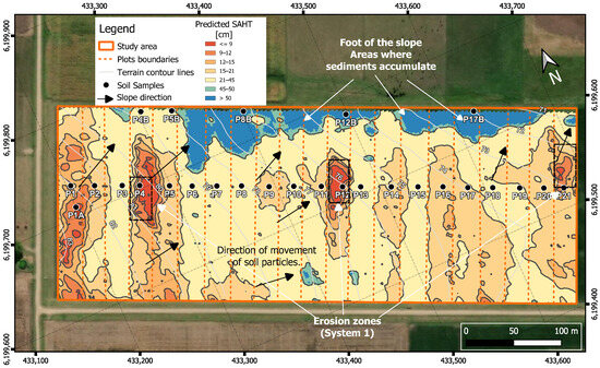
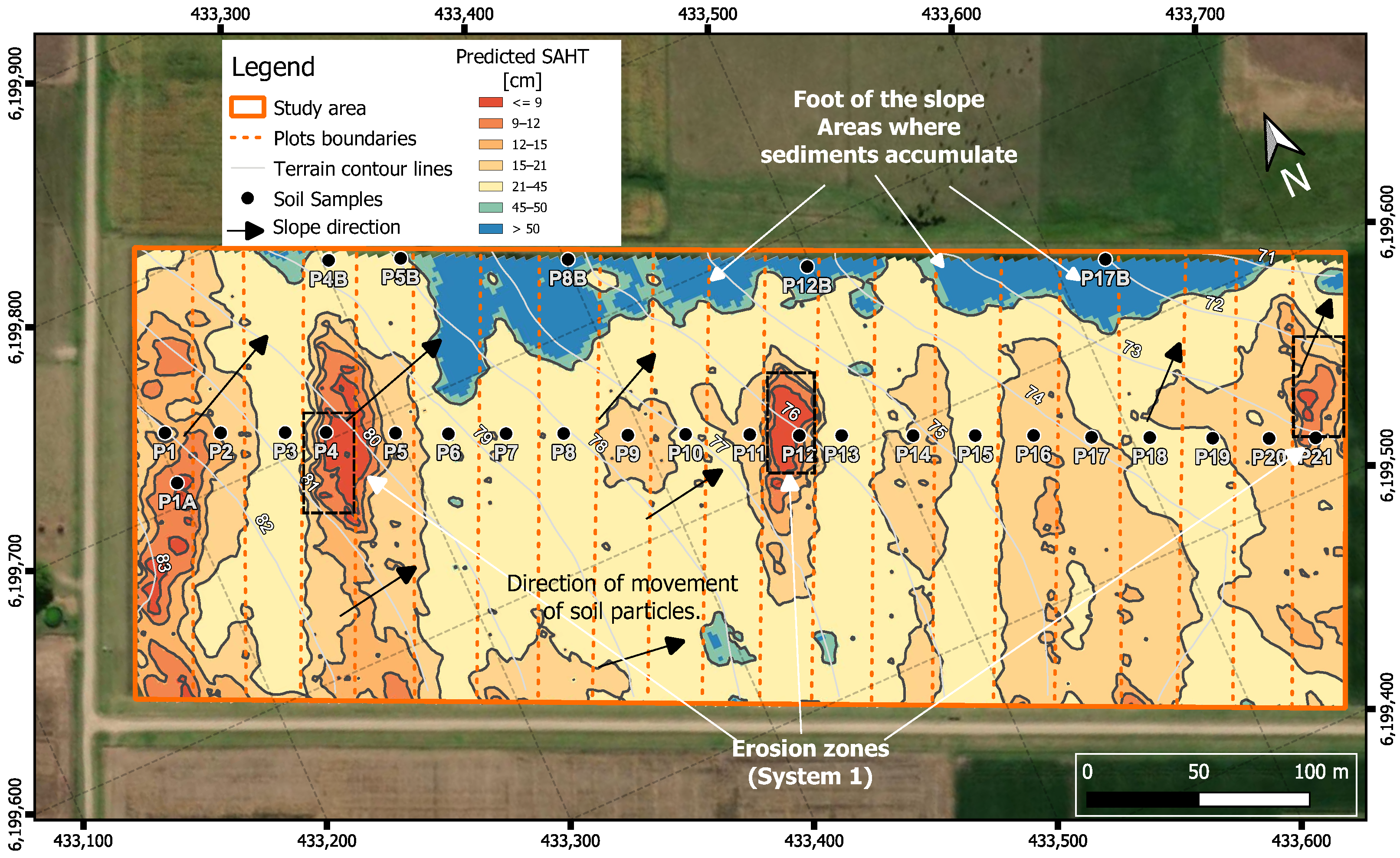
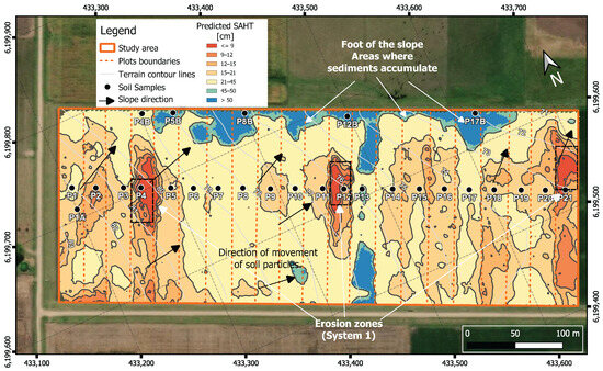
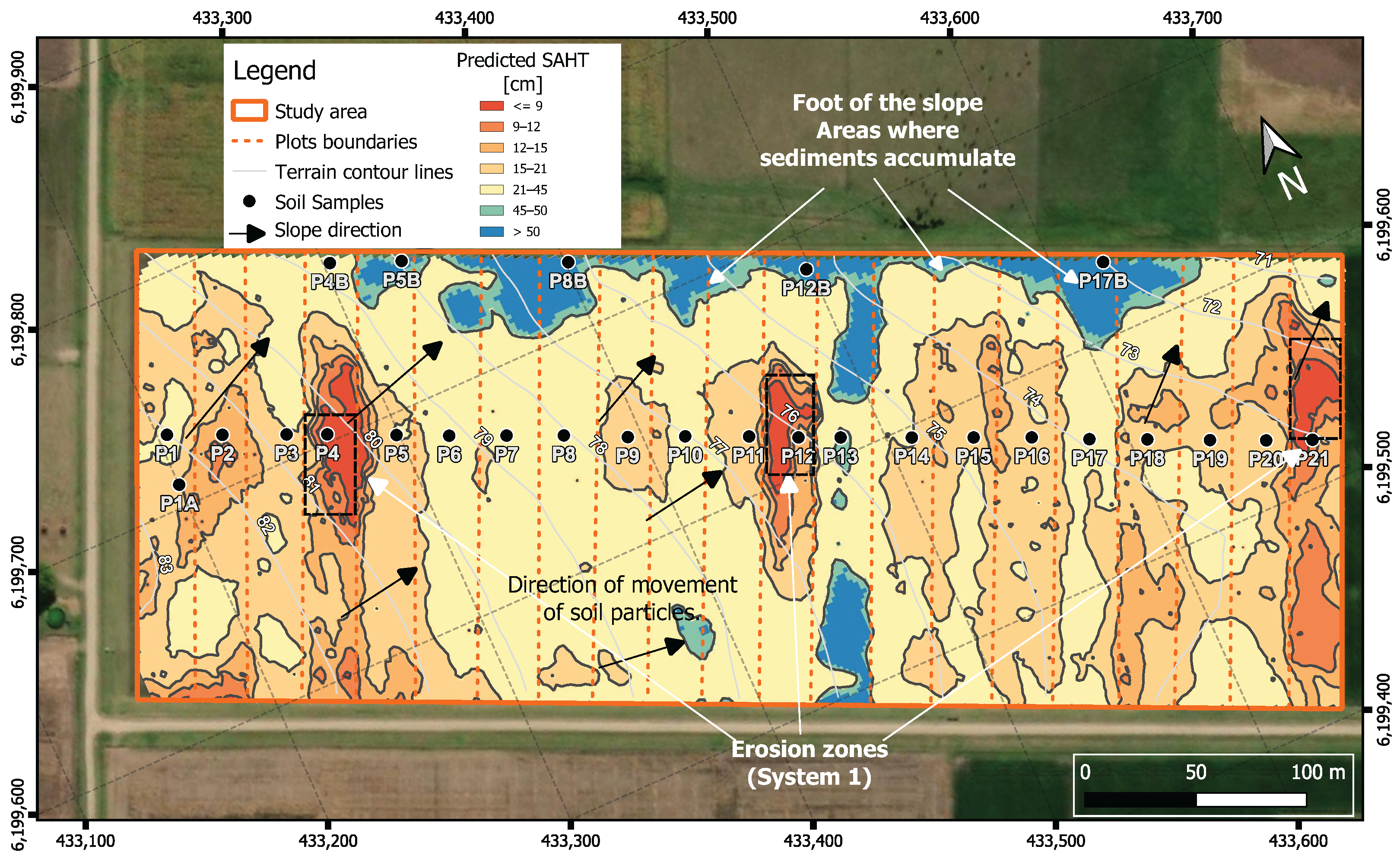
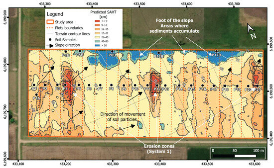
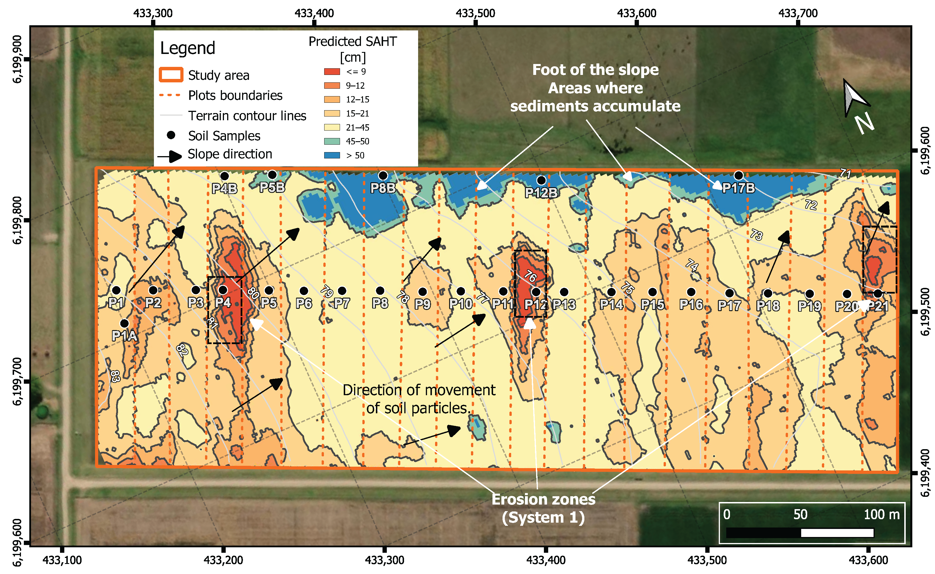
To analyze the generalization capacity of the model, a five-fold cross-validation strategy was used. The results showed stable and consistent performance across partitions, confirming the robustness of the model. Equation (3) was implemented in a Geographic Information System (GIS), using the electrical resistivity data shown in Figure 7. Figure 12 shows the resulting map, which predicts the SAHT across the entire area of the experiment.

Figure 12. Map of estimated soil A horizon thickness, excluding plots with vegetal cover in the calculations. The plots with vegetation cover are P1, P3, P6, and P15. Slope direction (black arrows) and gully erosion areas (black dashed boxes) are indicated.

3.5. SAHT Obtained from Other Soil Humidity Conditions

Equation (3) offers a simple and practical tool for obtaining the SAHT across La Estanzuela plots, from rapid EMI measurements. Since the model coefficients can vary under different overall soil conditions, especially of moisture content, it is important to recalculate them and validate the results in each situation. As an example of this, the previous procedures using data from a second measurement campaign were repeated, which was conducted under higher soil moisture conditions. The same interpolation criteria applied in Figure 7 were used here to visualize the EMI data. The resulting electrical resistivity map is shown in Figure 13.

Figure 13. Soil electrical resistivity map for a situation with higher moisture content in the soil than that corresponding to Figure 7. Gully erosion areas (black dashed boxes) are indicated.

This map reveals a general reduction in resistivity in relation to that shown in Figure 7, a logical consequence of the increase in soil moisture. In Figure 13, the plots with vegetation cover are P13 and P17.

Similar results to those in Table 5 were obtained in this case. The best resulting model also corresponded to the electrical resistivity variable, excluding the plots with vegetation cover. The mathematical relation between SAHT and electrical resistivity is:

$$\mathrm{SAHT}=2.82{\displaystyle \frac{\mathrm{cm}}{\Omega \mathrm{m}}}·\mathrm{RE}-41.98\mathrm{cm}$$

(4)

This model achieved an RMSE of $5.40$ cm and MAE of $4.17$ cm, with performance metrics $NSE=0.86$ and $R^2=0.86$. Compared to the previous model (Equation (3)), the parameters shifted, with the slope increasing from $2.06$ to $2.82$ and the y-intercept decreasing from $-29.40$ to $-41.98$, due to the change in soil moisture. Figure 14 illustrates the SAHT map computed using Equation (4) over the electrical resistivity distribution from Figure 13.

Figure 14. Map of estimated soil A horizon thickness, excuding plots with vegetal cover in the calculations, for larger overall moisture contents than in Figure 13. The plots with vegetation cover are P13 and P17. Slope direction (black arrows) and gully erosion areas (black dashed boxes) are indicated.

Comparing the maps of Figure 12 and Figure 14, it can be observed that the main differences in the SAHT prediction are found in the plots with the presence of vegetation cover. By disregarding these plots, this LRM satisfactorily adapted to different moisture conditions simply by recalculating the parameters. This characteristic allows the model to be transferred from one site or condition to another. However, under conditions substantially different from those of this study (interregional variations in soil structure, generalized or localized water saturation, etc.), adaptability could fail and the model may require reworking.

The maps of Figure 12 and Figure 14 were finally combined by averaging the predicted SAHT values, assigning zero weight to plots P1, P3, P6, and P15 in Figure 12 and to P13 and P17 in Figure 14. The resulting integrated map is showed in Figure 15.

Figure 15. Map of estimated soil A horizon thickness combining Figure 12 and Figure 14. Slope direction (black arrows) and gully erosion areas (black dashed boxes) are indicated.

The combined map provides a more robust representation for predicting SAHT ($R^2=0.90$) by integrating information from two independently calculated LRMs, corresponding to different soil humidity conditions and coverage. Averaging the predictions reduces the influence of local anomalies and model-specific biases, while assigning zero weight to plots with vegetation cover or inconsistent conditions minimizes error propagation. From a research perspective, this methodology is interesting because it allows for greater accuracy under different conditions of the plots. However, if applied at the grower scale, it would be advisable to survey only sites without vegetation cover, as well as other sources of important local fluctuations and general anomalous behavior of the geophysical data (e.g., water saturation conditions), to simplify data acquisition, increase precision, and reduce time and costs.

3.6. Relationship Between the SAHT and the Conservation State of the Plots

The lowest average values of SAHT per plot and most significant contrasts of this variable between plots are observed for the CA systems (P4, P12 and P21), which are known to be the most affected by erosion [16,56,59,60]. The first group of replicated plots (P1 to P7), the oldest in the series, is characterized by a greater dispersion of the mean SAHT values and a relatively low median. This dispersion appears to be primarily related to the location of these plots in the highest part of the experiment, where differential erosion processes would be generating complementary modifications. In particular, the SAHT of P4 indicates that this plot is the most deteriorated of the experiment (Figure 2 and Figure 3), in accordance with the information available from other sources. In the second repetition group (plots P8 to P14), the SAHT is on average moderately high and relatively homogeneous, except for an area located close to the center of P12 (CA), in which this variable is low, due to the presence of the aforementioned gullies (Figure 2). According to the SAHT, the plots that are most preserved in the second repetition group are P13 (${\mathrm{CPR}}_{66}$) and, in the second place, P11 (${\mathrm{CPR}}_{50}$). In the third repetition group (plots P15 to P21), the SAHT dispersion between plots is intermediate, and the SAHT median is comparable to that of the first repetition group. The lowest SAHT is observed in the central area of P21 (CA), whereas the highest values of SAHT correspond to P15, a ${\mathrm{CPR}}_{66}$ plot that is known to be one of the most preserved ones. The largest values of SAHT (SAHT > 45 cm) across the entire experiment are observed mainly in the northeast sector, where sediment accumulation is expected, as well as in small areas of P11 and P13, all of them under CPR treatments.

4. Conclusions

The integrated ERT, EMI, and core sampling methodology evaluated in this article proved to be reliable and efficient for estimating and mapping the SAHT within the La Estanzuela long-term experiment, for different scenarios with diverse pasture and fertilizer treatments, which are frequent in Uruguay and the region. ERT survey lines were strategically placed across the plots. A low-cost electrode mounting system was designed and constructed to streamline data acquisition, reducing the average setup time by 60% compared to manual handling. The ERT data, in conjunction with borehole data and pre-existing stratigraphic information on the site formations, allowed interpreting a series of soil profiles in terms of three main horizons, A, B and C, whose depth and width varied across the experiment. Strong correlations between the geophysical signals, core observations and pre-existing information were obtained.

Textural analysis confirmed this interpretation and revealed meaningful differences between the composition of the A, B and C horizons, with higher sand content in the A horizon, which explained its relatively elevated mean eletrical resistivity. EMI data, collected over a measurement grid covering the entire experiment, produced electrical resistivity maps that correlated well with zones of varying soil conditions, from degraded to well-conserved.

Regression models linking the EMI data to the ERT core observations enabled the generation of SAHT maps across the entire LTE. These maps revealed spatial (lateral and vertical) variability associated with the conservation status of the soil. Plots under continuous agriculture, regardless of fertilization, exhibited the lowest SAHT values and preservation status, while those under crop rotation with increasing pasture percentages showed progressively higher SAHT and preservation. The highest SAHT values were concentrated near the FOS area, consistent with the topographic accumulation processes that occurred there over more than 60 years of the experiment, whereas the lowest SAHT values agree with highly eroded areas that often showed marked gullies.

When comparing SAHT maps corresponding to acquisition periods with different humidity in the soil, similar values of SAHT were observed for plots without vegetation cover, which indicated consistent modeling results in these areas. The most significant variations appear in plots with vegetation, where the presence of plant cover likely introduced fluctuations and noise into the geophysical data. This suggested the exclusion of vegetated plots in the mapping input. This alternative procedure improved the results. Combining the resulting maps further improved the final precision in areas under bare soil conditions. As the evaluated methodology performs best under these types of conditions, future applications to experimental or farmer-managed plots should prioritize data collection during periods of minimal vegetation cover in order to improve accuracy, avoiding circumstances that could increase local fluctuations or produce generalized anomalous behavior of the geophysical data. Since scaling up beyond experimental plots will be required, we recommend increasing the number of ERT measurements and soil-coring samples at anomalies detected after generating resistivity maps with EMI. This strategy enhances resolution and reliability over larger areas. In addition, adapting the electrode mounting system to a tractor’s three-point hydraulic hitch can further reduce operator effort and improve the feasibility of extensive field coverage.

Mapping the SAHT through the considered physical measurements provided essential information for optimizing crop productivity and guiding sustainable soil management. The presented methodology is expected to contribute, in a simple, rapid (i.e., approximately 0.1 ${\mathrm{km}}^2$ of land prospected in less than a day), and cost-effective way, to agricultural practices in La Estanzuela LTE, as well as to similar environments that can be represented as a two-layer system in the EMI measurements.

References

- Hartemink, A.; Zhang, Y.; Bockheim, J.; Curi, N.; Silva, S.; Grauer-Gray, J.; Lowe, D.J.; Krasilnikov, P. Soil horizon variation: A review. Adv. Agron. 2020, 160, 125–185. [Google Scholar]
- Power, J.; Sandoval, F.; Ries, R.; Merrill, S. Effects of topsoil and subsoil thickness on soil water content and crop production on a disturbed soil. Soil Sci. Soc. Am. J. 1981, 45, 124–129. [Google Scholar] [CrossRef] [Scilit]
- Arriaga, F.; Lowery, B. Erosion and productivity. In Encyclopedia of Water Science; CRC Press: New York, NY, USA, 2003; pp. 222–224. [Google Scholar]
- Suleymanov, A.; Komissarov, M.; Asylbaev, I.; Khasanov, A.; Khabirov, I.; Suleymanov, R.; Gabbasova, I.; Belan, L.; Tuktarova, I. Spatial Variations of Genetic Horizons Thicknesses and Erosion Degree Assessment in Temperate Soils. Environ. Process. 2024, 11, 44. [Google Scholar] [CrossRef] [Scilit]
- Groppelli, E.; Giampaoli, O. Biodigestores: Una Propuesta Sustentable; Ediciones UNL, Universidad Nacional del Litoral: Santa Fe, Argentina, 2012. [Google Scholar]
- FAO. Global Symposium on Soil Erosion. 2020. Available online: https://esdac.jrc.ec.europa.eu/node/66983 (accessed on 4 February 2025).
- Amangabara, G.T. Understanding effective gully control measures in Imo State, Nigeria. Can. Open Soil Eros. J. 2014, 1, 1–9. [Google Scholar]
- Conforti, M.; Longobucco, T.; Scarciglia, F.; Niceforo, G.; Matteucci, G.; Buttafuoco, G. Interplay between soil formation and geomorphic processes along a soil catena in a Mediterranean mountain landscape: An integrated pedological and geophysical approach. Environ. Earth Sci. 2020, 79, 59. [Google Scholar] [CrossRef] [Scilit]
- Nath, A.; Bhuyan, P.; Gogoi, N.; Deka, P. Pesticides and Chemical Fertilizers: Role in Soil Degradation, Groundwater Contamination, and Human Health. In Xenobiotics in Urban Ecosystems: Sources, Distribution and Health Impacts; Singh, R., Singh, P., Tripathi, S., Chandra, K.K., Bhadouria, R., Eds.; Springer International Publishing: Cham, Switzerland, 2023; pp. 131–160. [Google Scholar] [CrossRef] [Scilit]
- Musa, I.O.; Samuel, J.O.; Adams, M.; Abdulsalam, M.; Nathaniel, V.; Maude, A.M.; Adedayo, O.A.; Tiamiyu, A.T. Soil Erosion, Mineral Depletion and Regeneration. In Prospects for Soil Regeneration and Its Impact on Environmental Protection; Springer Nature Switzerland: Cham, Switzerland, 2024; pp. 159–172. [Google Scholar] [CrossRef] [Scilit]
- Baridón, J.E.; Marlats, R.M.; Lanfranco, J.W.; Pellegrini, A.E. Productividad de Populus deltoides en Argiudoles y Hapludoles de la Pampa Húmeda: Relación con índices indirectos de sitio. Quebracho 2005, 12, 43–53. [Google Scholar]
- Alvarez, R.; Taboada, M.; Gutierrez Boem, F. Changes in the porosity induced by tillage in typical Argiudolls of southeastern Buenos Aires Province, Argentina. Environ. Earth Sci. 2018, 77, 134. [Google Scholar] [CrossRef] [Scilit]
- Durán, A.; Califra, A.; Molfino, J. Suelos del Uruguay según Soil Taxonomy; Ministerio de Ganadería, Agricultura y Pesca, Dirección General de Recursos Naturales: Montevideo, Uruguay, 1999. [Google Scholar]
- Wilson, M.G.; Maggi, A.E.; Castiglioni, M.G.; Gabioud, E.A.; Sasal, M.C. Conservation of Ecosystem Services in Argiudolls of Argentina. Agriculture 2020, 10, 649. [Google Scholar] [CrossRef] [Scilit]
- Sainato, C.; Losinno, B.; Márquez Molina, J.; Espada, R. Electromagnetic soundings to detect groundwater contamination produced by intensive livestock farming. J. Appl. Geophys. 2018, 154, 159–166. [Google Scholar] [CrossRef] [Scilit]
- Grahmann, K.; Terra, J.A.; Ellerbrock, R.; Rubio, V.; Barro, R.; Caamaño, A.; Quincke, A. Data accuracy and method validation of chemical soil properties in long-term experiments: Standard operating procedures for a non-certified soil laboratory in Latin America. Geoderma Reg. 2022, 28, e00487. [Google Scholar] [CrossRef] [Scilit]
- Durán, A.; Califra, A.; Molfino, J. Suelos del Uruguay según Soil Taxonomy (1999); Technical Report; Facultad de Agronomía, Universidad de la República: Montevideo, Uruguay, 2006. [Google Scholar]
- Chaplot, V.; Lorentz, S.; Podwojewski, P.; Jewitt, G. Digital mapping of A-horizon thickness using the correlation between various soil properties and soil apparent electrical resistivity. Geoderma 2010, 157, 154–164. [Google Scholar] [CrossRef] [Scilit]
- Farooq, O.; Imran, M.; Awan, M.I.; Sarwar, N.; Mubeen, K.; Ahmed, M.; Ahmad, S. Causes of Soil Erosion, Its Measurements, and Management. In Disaster Risk Reduction in Agriculture; Springer Nature: Singapore, 2023; pp. 211–232. [Google Scholar] [CrossRef] [Scilit]
- Ferro, V.; Nicosia, A. Soil Erosion Measurement Techniques and Field Experiments. Water 2023, 15, 2846. [Google Scholar] [CrossRef] [Scilit]
- Catanha, M.; Sacasas León, C.; Pérez Lazo, J. Criterios para localizar zonas acuíferas en Caimbambo, Angola. Ing. Hidráulica Y Ambient. 2014, 35, 45–52. [Google Scholar]
- Čupić, A.; Smičiklas, I.; Manić, M.; Đokić, M.; Dragović, R.; Đorđević, M.; Gocić, M.; Jović, M.; Topalović, D.; Gajić, B.; et al. 137Cs-Based Assessment of Soil Erosion Rates in a Morphologically Diverse Catchment with Varying Soil Types and Vegetation Cover: Relationship with Soil Properties and RUSLE Model Predictions. Water 2025, 17, 526. [Google Scholar] [CrossRef] [Scilit]
- Porto, P.; Fulajtar, E.; Heng, L.K. Using 137Cs Resampling Method to Estimate Mean Soil Erosion Rates for Selected Time Windows; Springer: Cham, Switerland, 2024. [Google Scholar]
- Pereira, G.W.; Valente, D.S.M.; de Queiroz, D.M.; Santos, N.T.; Fernandes-Filho, E.I. Soil mapping for precision agriculture using support vector machines combined with inverse distance weighting. Precis. Agric. 2022, 23, 1189–1204. [Google Scholar] [CrossRef] [Scilit]
- Telford, W.M.; Geldart, L.P.; Sheriff, R.E. Applied Geophysics; Cambridge University Press: Cambridge, UK, 1990. [Google Scholar]
- Tabbagh, A.; Dabas, M.; Hesse, A.; Panissod, C. Soil resistivity: A non-invasive tool to map soil structure horizonation. Geoderma 2000, 97, 393–404. [Google Scholar] [CrossRef] [Scilit]
- Besson, A.; Cousin, I.; Samouëlian, A.; Boizard, H.; Richard, G. Structural heterogeneity of the soil tilled layer as characterized by 2D electrical resistivity surveying. Soil Tillage Res. 2004, 79, 239–249. [Google Scholar] [CrossRef] [Scilit]
- Wang, T.P.; Chen, C.C.; Tong, L.T.; Chang, P.Y.; Chen, Y.C.; Dong, T.H.; Liu, H.C.; Lin, C.P.; Yang, K.H.; Ho, C.J.; et al. Applying FDEM, ERT and GPR at a site with soil contamination: A case study. J. Appl. Geophys. 2015, 121, 21–30. [Google Scholar] [CrossRef] [Scilit]
- Hernandez, J.P.; González, A.P.; Díaz, E.L. Evaluación de la distribución de humedad en la zona no saturada mediante calicata eléctrica, Oro Verde, Entre Ríos, Argentina. In Proceedings of the Estudios en la Zona No Saturada del Suelo–Vol. XIII (ZNS’17), Zaragoza, Spain, 8–10 November 2017. [Google Scholar]
- Heil, K.; Schmidhalter, U. Theory and Guidelines for the Application of the Geophysical Sensor EM38. Sensors 2019, 19, 4293. [Google Scholar] [CrossRef] [Scilit] [PubMed]
- Ünal, I.; Kabaş, Ö.; Sözer, S. Real-time electrical resistivity measurement and mapping platform of the soils with an autonomous robot for precision farming applications. Sensors 2020, 20, 251. [Google Scholar] [CrossRef] [Scilit]
- Pathirana, S.; Lambot, S.; Krishnapillai, M.; Cheema, M.; Smeaton, C.; Galagedara, L. Ground-Penetrating Radar and Electromagnetic Induction: Challenges and Opportunities in Agriculture. Remote Sens. 2023, 15, 2932. [Google Scholar] [CrossRef] [Scilit]
- Delgado Rodríguez, O.; Ladrón de Guevara Torres, M.; Shevnin, V.; Ryjov, A. Estimation of soil petrophysical parameters based on electrical resistivity values obtained from lab and in-field measurements. Geofísica Int. 2012, 51, 5–15. [Google Scholar] [CrossRef]
- Lund, E.; Christy, C.; Drummond, P. Practical applications of soil electrical conductivity mapping. Precis. Agric. 1999, 99, 771–779. [Google Scholar]
- Dabas, M. Theory and practice of the new fast electrical imaging system ARP©. In Seeing the Unseen. Geophysics and Landscape Archaeology; CRC Press: Boca Raton, FL, USA, 2008; pp. 131–154. [Google Scholar]
- Dabas, M.; Hesse, A.; Jolivet, A. Prospection électrique de subsurface automatisée. Aer. Photogr. Geophys. Prospect. Archaeol. 1990, 2, 73–81. [Google Scholar]
- Moral, F.J.; Rebollo, F.J.; Serrano, J.M.; Carvajal, F. Mapping management zones in a sandy pasture soil using an objective model and multivariate techniques. Precis. Agric. 2021, 22, 800–817. [Google Scholar] [CrossRef] [Scilit]
- Virk, S.S.; Porter, W.M.; Li, C.; Rains, G.C.; Snider, J.L.; Whitaker, J.R. On-farm evaluation of planter downforce in varying soil textures within grower fields. Precis. Agric. 2021, 22, 777–799. [Google Scholar] [CrossRef] [Scilit]
- Aizebeokhai, A.P. 2D and 3D geoelectrical resistivity imaging: Theory and field design. Sci. Res. Essays 2010, 5, 3592–3605. [Google Scholar]
- Boiarskii, B.; Vaitekhovich, I.; Tanaka, S.; Güneş, D.; Sato, T.; Hasegawa, H. Comparative Analysis of Remote Sensing via Drone and On-the-Go Soil Sensing via Veris U3: A Dynamic Approach. Environ. Sci. Proc. 2024, 29, 11. [Google Scholar] [CrossRef] [Scilit]
- Rossi, R.; Pollice, A.; Diago, M.P.; Oliveira, M.; Millan, B.; Bitella, G.; Amato, M.; Tardaguila, J. Using an Automatic Resistivity Profiler Soil Sensor On-The-Go in Precision Viticulture. Sensors 2013, 13, 1121–1136. [Google Scholar] [CrossRef] [Scilit] [PubMed]
- Dabas, M.; Decriaud, J.P.; Ducomet, G.; Hesse, A.; Mounir, A.A.; Tabbagh, A. Continuous recording of resistivity with towed arrays for systematic mapping of buried structures at shallow depths. ArchéoSciences Rev. D’Archéométrie 1994, 18, 13–17. [Google Scholar] [CrossRef] [Scilit]
- Uhlemann, S.; Wilkinson, P.B.; Maurer, H.; Wagner, F.M.; Johnson, T.C.; Chambers, J.E. Optimized survey design for electrical resistivity tomography: Combined optimization of measurement configuration and electrode placement. Geophys. J. Int. 2018, 214, 108–121. [Google Scholar] [CrossRef] [Scilit]
- de Vetten, L. A comparison of Methods Assessing Soil Compaction on Black Vertosols. South-Eastern Queensland, Australia. Ph.D. Thesis, Wageningen University, Wageningen, The Netherlands, 2014. [Google Scholar]
- Sainato, C.M.; Losinno, B.N.; Malleville, H.J. Electrical resistivity tomography applied to detect contamination on a dairy farm in the Pampean region, Argentina. Surf. Geophys. 2010, 8, 163–171. [Google Scholar] [CrossRef] [Scilit]
- Dietrich, S.; Weinzettel, P.A.; Varni, M. Infiltration and drainage analysis in a heterogeneous soil by electrical resistivity tomography. Soil Sci. Soc. Am. J. 2014, 78, 1153–1167. [Google Scholar] [CrossRef] [Scilit]
- Giménez, M.; Menta, A.; Ramos, J.; Musso, M.; Flaquer, A. Aplicación de métodos geofísicos al estudio del sistema hidrogeológico Libertad Raigón de Uruguay. Boletín Geológico Y Min. 2020, 132, 185–196. [Google Scholar] [CrossRef] [Scilit]
- de Mello, D.C.; Ferreira, T.O.; Veloso, G.V.; de Lana, M.G.; de Oliveira Mello, F.A.; Di Raimo, L.A.D.L.; Cabrero, D.R.O.; de Souza, J.J.L.L.; Fernandes-Filho, E.I.; Francelino, M.R.; et al. Digital mapping of soil weathering using field geophysical sensor data coupled with covariates and machine learning. J. S. Am. Earth Sci. 2023, 128, 104449. [Google Scholar] [CrossRef] [Scilit]
- Mansourian, D.; Vanderhasselt, A.; Cornelis, W.; Hermans, T. Response to soil compaction of the electrical resistivity tomography, induced polarisation, and electromagnetic induction methods: A case study in Belgium. Soil Res. 2023, 62, SR22260. [Google Scholar] [CrossRef] [Scilit]
- Paz, M.C.; Castanheira, N.L.; Paz, A.M.; Gonçalves, M.C.; Monteiro Santos, F.; Farzamian, M. Comparison of electromagnetic induction and electrical resistivity tomography in assessing soil salinity: Insights from four plots with distinct soil salinity levels. Land 2024, 13, 295. [Google Scholar] [CrossRef] [Scilit]
- Kaufmann, M.S.; Klotzsche, A.; van der Kruk, J.; Langen, A.; Vereecken, H.; Weihermüller, L. Assessing soil fertilization effects using time-lapse electromagnetic induction. Soil 2025, 11, 267–285. [Google Scholar] [CrossRef] [Scilit]
- Garré, S.; Javaux, M.; Vanderborght, J.; Pagès, L.; Vereecken, H. Three-dimensional electrical resistivity tomography to monitor root zone water dynamics. Vadose Zone J. 2011, 10, 412–424. [Google Scholar] [CrossRef] [Scilit]
- Cassiani, G.; Boaga, J.; Vanella, D.; Perri, M.T.; Consoli, S. Monitoring and modelling of soil–plant interactions: The joint use of ERT, sap flow and eddy covariance data to characterize the volume of an orange tree root zone. Hydrol. Earth Syst. Sci. 2015, 19, 2213–2225. [Google Scholar] [CrossRef] [Scilit]
- Carrera, A.; Longo, M.; Piccoli, I.; Mary, B.; Cassiani, G.; Morari, F. Electro-magnetic geophysical dynamics under conservation and conventional farming. Remote Sens. 2022, 14, 6243. [Google Scholar] [CrossRef] [Scilit]
- Grahmann, K.; Rubio, V.; Perez-Bidegain, M.; Quincke, J.A. Soil Use Legacy as Driving Factor for Soil Erosion under Conservation Agriculture. Front. Environ. Sci. 2022, 10, 822967. [Google Scholar] [CrossRef] [Scilit]
- Quincke, A.; Ciganda, V.; Sawchik, J.; Fernández, E.; Hirigoyen, D.; Sotelo, D.; Restaino, E.; Lapetina, J. Rotaciones cultivos pasturas INIA La Estanzuela: Aprendiendo del experimento más antiguo de Latinoamérica. Rev. INIA 2019, 59, 46–60. [Google Scholar]
- Morón, A. Efecto de las rotaciones Cultivos-Pasturas sobre la fertilidad de los suelos en ensayos de larga duración del INIA La Estanzuela (1963–2003). Inf. Agronómicas 2003, 20, 1–20. [Google Scholar]
- IDEUY. Digital Elevation Model; Spatial Data Infrastructure of Uruguay: Montevideo, Uruguay, 2023. [Google Scholar]
- Grahmann, K.; Rubio Dellepiane, V.; Terra, J.A.; Quincke, J.A. Long-term observations in contrasting crop-pasture rotations over half a century: Statistical analysis of chemical soil properties and implications for soil sampling frequency. Agric. Ecosyst. Environ. 2020, 287, 106710. [Google Scholar] [CrossRef] [Scilit]
- Rubio, V.; Diaz-Rossello, R.; Quincke, J.A.; van Es, H.M. Quantifying soil organic carbon’s critical role in cereal productivity losses under annualized crop rotations. Agric. Ecosyst. Environ. 2021, 321, 107607. [Google Scholar] [CrossRef] [Scilit]
- Casabella-González, M.; Borselli, L.; García-Meza, J. Soil Horizon erodibility assessment in an area of México susceptible to gully erosion. J. S. Am. Earth Sci. 2021, 111, 103497. [Google Scholar] [CrossRef] [Scilit]
- Ministerio de Ganadería, Agricultura y Pesca, MGAP. Carta de Suelos del Uruguay: Nueva Actualización; Ministerio de Ganadería, Agricultura y Pesca, MGAP: Montevideo, Uruguay, 2024. [Google Scholar]
- Preciozzi, F.; Sportuno, J.; Heinze, W.; Rossi, P. Carta Geológica del Uruguay; Dirección Nacional de Minería y Geología (DINAMIGE): Montevideo, Uruguay, 1985. [Google Scholar]
- Musso, M.; Rostán, A.; Behak, L. Subrasantes expansivas en Rutas Nacionales:¿ mito o realidad. In Proceedings of the Congreso de Ingeniería Vial, Asociación Uruguaya de Caminos, Montevideo, Uruguay, 4–6 November 2003; pp. 4–6. [Google Scholar]
- Cherry, J.A.; Freeze, R.A. Groundwater; Prentice-Hall: Englewood Cliffs, NJ, USA, 1979. [Google Scholar]
- Rodríguez, R.; Bango, G.; Flaquer, A.; Musso, M. Propiedades hidráulicas de la Fm. Libertad: Ensayos de Campo y Laboratorio. In Proceedings of the Actas XX Congreso Argentino de Geología, SM Tucumán, Argentina, 7–11 August 2017; p. 5. [Google Scholar]
- Menta Romano, A. Aplicación de Tomografía eléCtrica (ERT2D), Polarización Inducida (IP2D) y Muestreos geoquíMicos Para la Detección de Filtraciones de Lagunas de Efluentes de Establecimientos Lecheros. Master’s Thesis, Universidad Nacional Autónoma de México, Mexico City, Mexico, 2021. [Google Scholar]
- Doolittle, J.A.; Brevik, E.C. The use of electromagnetic induction techniques in soils studies. Geoderma 2014, 223, 33–45. [Google Scholar] [CrossRef] [Scilit]
- McNeeill, J. Electromagnetic Terrain Conductivity Measurement at Low Induction Numbers; Geonics Technical Note TN-6; Geonics Ltd.: Mississauga, ON, Canada, 1980. [Google Scholar]
- Wodajo, L.T.; Bakhtiari Rad, P.; Sharif, S.I.; Samad, M.A.; Mamud, M.L.; Hickey, C.J.; Wilson, G.V. Agrogeophysical methods for identifying soil pipes. J. Appl. Geophys. 2021, 192, 104383. [Google Scholar] [CrossRef] [Scilit]
- Geonics Limited. EM38-MK2 User Manual, 2nd ed.; Geonics Limited: Toronto, ON, Canada, 2025. [Google Scholar]
- Ciani, L.; Patrizi, G.; Innocenti, A.; Fanti, R.; Pazzi, V. Considerations on the electrode-spacing-to-electrode-diameter ratio in electrical resistivity tomography (ERT): An operational approach. IEEE Trans. Instrum. Meas. 2024, 73, 1–12. [Google Scholar] [CrossRef] [Scilit]
- Loke, M. Res2DInv ver. 3.59. 102 Geoelectrical Imaging 2D and 3D. Instruction Manual; Geotomo Software: Gelugor, Malaysia, 2010. [Google Scholar]
- Museo Virtual de Suelos. Brunosol Éutrico Típico. 2023. Available online: https://museovirtualdesuelos.net/perfiles-exhibidos/ (accessed on 15 November 2023).
- Soares Gerscovich, D.M.; Vipulanandan, C. Data analyses to correlate the soil properties to the electrical resistivity. Geotech. Geol. Eng. 2023, 41, 4507–4528. [Google Scholar] [CrossRef] [Scilit]
- Sangprasat, K.; Puttiwongrak, A.; Inazumi, S. Review of Correlations Between Soil Electrical Resistivity and Geotechnical Properties. Geosciences 2025, 15, 166. [Google Scholar] [CrossRef] [Scilit]
- Beretta, A.N.; Silbermann, A.V.; Paladino, L.; Torres, D.; Kassahun, D.; Musselli, R.; Lamohte, A.G. Soil texture analyses using a hydrometer: Modification of the Bouyoucos method. Cienc. E Investig. Agrar. Rev. Latinoam. De Cienc. De La Agric. 2014, 41, 263–271. [Google Scholar] [CrossRef] [Scilit]
- Moeys, J.; Shangguan, W.; Petzold, R.; Minasny, B.; Rosca, B.; Jelinski, N.; Zelazny, W.; Souza, R.M.S.; Safanelli, J.L.; ten Caten, A. Soiltexture: Functions for Soil Texture Plot, Classification and Transformation, R Package Version 1.5.3. 2024. Available online: https://cran.r-project.org/web/packages/soiltexture/index.html (accessed on 10 December 2025).
- Jiménez, J.U. Funciones para Graficar en R; Centro de Investigaciones Hidráulicas e Hidrotécnicas, Universidad Tecnológica de Panamá: Panama City, Panama, 2019. [Google Scholar]
- Peinado-Guevara, H.J.; Green-Ruíz, C.R.; Delgado-Rodríguez, O.; Herrera-Barrientos, J.; Belmonte-Jiménez, S.; Ladrón de Guevara Torres, M.d.l.A.; Shevnin, V. Estimación de la conductividad hidráulica y contenido de finos a partir de leyes experimentales que relacionan parámetros hidráulicos y eléctricos. Ra Ximhai 2010, 6, 469–478. [Google Scholar] [CrossRef] [Scilit]
- Driba, D.; Emmanuel, E.; Doro, K. Predicting wetland soil properties using machine learning, geophysics, and soil measurement data. J. Soils Sediments 2024, 24, 2398–2415. [Google Scholar] [CrossRef] [Scilit]
- Nachtigall, S.D.; Reis, R.A.; Mancini, M.; de Araújo, E.F.; Carneiro, M.A.C.; Curi, N.; Silva, S.H.G. Advancing the transferability of local and regional soil texture prediction models based on X-ray fluorescence. J. South Am. Earth Sci. 2025, 164, 105629. [Google Scholar] [CrossRef] [Scilit]
Disclaimer/Publisher’s Note: The statements, opinions and data contained in all publications are solely those of the individual author(s) and contributor(s) and not of MDPI and/or the editor(s). MDPI and/or the editor(s) disclaim responsibility for any injury to people or property resulting from any ideas, methods, instructions or products referred to in the content. |
© 2026 by the authors. Licensee MDPI, Basel, Switzerland. This article is an open access article distributed under the terms and conditions of the Creative Commons Attribution (CC BY) license.