


Abstract
This set of notes complements the lectures and recitation sessions discussed in the following graduate schools: Hampton University Graduate Summer Program (HUGS) at Jefferson Lab (years 2018, 2019, 2021), the International School and Workshop on Probing Hadron Structure at the Electron-Ion Collider at International Centre for Theoretical Sciences (ICTS) (2024), Frontiers in Nuclear and Hadronic Physics at The Galileo Galilei Institute for Theoretical Physics (GGI) (2025), and the International Workshop and School on Hadron Structure and Strong Interactions at Nanjing University (2025).
1. Introduction
These lecture notes are essentially a written version of the lectures and recitation sessions that were delivered at the HUGS (https://www.jlab.org/stem/hugs (accessed on 3 April 2026)) program at Jefferson Lab (years 2018, 2019, 2021), the International School and Workshop on Probing Hadron Structure at the Electron-Ion Collider (https://icts.res.in/program/QEICIII2024 (accessed on 3 April 2026)) at ICTS (2024), Frontiers in Nuclear and Hadronic Physics (https://www.ggi.infn.it/showevent.pl?id=494 (accessed on 3 April 2026)) at GGI (2025), and the International Workshop and School on Hadron Structure and Strong Interactions (https://indico.ihep.ac.cn/event/27023/ (accessed on 3 April 2026)) at Nanjing University (2025).
The aim of these notes is not to provide a comprehensive overview of the topic of hadron tomography in momentum space, but to provide a guide, a map for newcomers to find an accessible entry point and to be able to position themselves in relation to the vast literature and research directions within this exciting research field. Training the next generation of scientists is an essential step in moving science forward. Often graduate students learn directly from research articles, which are rarely written in a pedagogical way. In this respect, providing an entry-level manual to tackle the field of hadronic imaging in momentum space is a worthwhile initiative.
The lecture notes are organized as follows. In Section 1, we briefly introduce the distribution functions that encode information on the structure of hadrons and a selection of suggested references is given. In Section 2, we present the process of Deep-Inelastic Scattering (DIS) and the response functions used to parametrize the structure of the target. In Section 3, we introduce transverse momentum distributions and discuss Semi-Inclusive DIS, as a tool to investigate the dependence on partonic transverse momentum in the description of the hadronic target and of the produced hadron. In Section 4, we discuss the interplay between the gauge and discrete symmetries which give rise to spin–momentum correlations that obey generalized universality properties. In Section 5, we briefly present some of the steps needed to establish an imaging program relying on perturbation theory, namely, the concept of TMD evolution and the relevance of emerging non-perturbative effects in TMD observables.
1.1. The Hadron Structure Landscape
In these lecture notes, we will focus mostly on collinear and transverse-momentum-dependent distribution functions and fragmentation functions. However, these quantities are part of a much broader and richer landscape of functions that characterize hadron structure and hadronization within the framework of Quantum Chromodynamics (QCD). At the most general level, one can introduce generalized parton correlation functions (see Equation (1)), which depend simultaneously on the partonic four momentum k, the four momentum P of the hadronic target, and the four momentum transferred to the final-state hadron. For a two-quark correlation function the definition reads [1]:
where the ket and bra are momentum eigenstates of the hadronic target, is the Dirac field of the struck quark, z is the space-time separation conjugated to the momentum k, and the Dirac matrix selects a specific Dirac projection (as will be explained in more detail in the forthcoming sections). For now, we do not consider the additional complications associated with the gauge invariance and the renormalization of these objects. Figure 1 provides a graphical representation of Equation (1), in which a quark with four momentum is extracted from a hadron target with four momentum and is then reabsorbed into the bound state transferring a four-momentum imbalance .
Figure 1.
Graphical representation of the parton correlation function defined in Equation (1). The labels indicate the momentum assignments for the quarks and the hadrons.
By taking suitable limits, Fourier transforms, and projections of the parent correlation function , one can obtain a number of distributions that appear in the context of hadron tomography. Figure 2 gives a graphical representation of the connection between H and these other distributions. For example, setting the momentum transfer to zero and then integrating over the suppressed quark momentum component leads to transverse-momentum-dependent distributions (TMDs), which provide a three-dimensional picture of hadrons in momentum space. Additionally integrating over the partonic transverse momentum yields the simpler collinear parton distribution functions (PDFs). Alternatively, integrating H over and over the transverse momentum while retaining a finite momentum transfer leads to the generalized parton distributions (GPDs [1,2,3]). These functions describe the spatial distribution of partons inside hadrons, and are connected with impact-parameter distributions and form factors. Last but not least, Wigner distributions and generalized transverse-momentum-dependent distributions (GTMDs) combine information on both momentum and position [4]. Figure 2 summarizes these relations schematically, emphasizing how the different functions are interconnected through well-defined mathematical operations rather than representing independent descriptions of hadron structure.
Figure 2.
Selected quantities that can be derived from the parton correlation function (PCF) defined in Equation (1). Double arrows marked by “FT” denote a Fourier transform between and or between and . Fractions of plus-momentum (commonly called “longitudinal momentum fractions”) are written as and . The scales introduced by ultraviolet renormalization or by the regulation of rapidity divergences are suppressed. As discussed in the text, the integrals cannot be taken literally but must be supplemented with a regularization procedure. Figure inspired by Ref. [1]. Acronyms: PCF (parton correlation function), GTMD (generalized transverse momentum distribution), GPD (generalized parton distribution), GFF (generalized form factor), TMD (transverse momentum distribution), PDF (parton distribution function).
Although the function in Equation (1) provides the most general description of the quark correlation function, no phenomenologically established process is currently known to probe it directly through a factorization theorem. Existing factorization frameworks involve only lower-dimensional projections of H, such as PDFs, TMDs, GTMDs, or GPDs. Thus, the partonic structure of hadrons can be investigated by combining information from different projections of the same underlying structure [4].
A word of caution is in order before concluding this introduction. The integrations shown schematically in Figure 2 are formally valid for bare (unrenormalized) correlation functions. Once ultraviolet and rapidity divergences are taken into account, the definition of the physical distributions requires appropriate regularization and renormalization schemes [5]. As a consequence, some of the simple integral relations suggested by the figure receive important qualifications, and understanding how the different renormalized hadronic distributions are connected is still the subject of ongoing theoretical research [6].
1.2. Suggested References
As mentioned above, these notes are far from being a complete introduction to the field. Several important topics are missing or just introduced without delving into the details. To compensate for that, here a selection of additional resources is provided, organized by type.
1.2.1. Graduate Schools Lecture Notes
- R. Jaffe, Erice School Lecture Notes (https://arxiv.org/pdf/hep-ph/9602236.pdf (accessed on 3 April 2026)) [7]
- P. Mulders, GGI Lecture Notes (http://www.nat.vu.nl/~mulders/tmdreview-vs3.pdf (accessed on 3 April 2026)) [8]
- C. D. Roberts, Three Lectures on Hadron Physics (https://inspirehep.net/literature/1392805 (accessed on 3 April 2026)) [9]
- V. Barone, Cabeo Lecture Notes (https://www.fe.infn.it/cabeo_school/2010/cabeo_school_2010.pdf (accessed on 3 April 2026))
- A. Bacchetta, Trento Lecture Notes (https://www2.pv.infn.it/bacchett/teaching/Bacchetta_Trento2012.pdf (accessed on 3 April 2026)) [10]
- The HUGS Pedagogical Page (https://www.jlab.org/education/hugs/references (accessed on 3 April 2026))
1.2.2. Books
- V. Barone and P. Ratcliffe, Transverse Spin Physics
- J. Collins, Foundations of Perturbative QCD [5]
- R. Devenish and A. Cooper-Sarkar, Deep Inelastic Scattering
- T. Muta, Foundations of Quantum Chromodynamics [11]
- M. Peskin, D. Schroeder, An Introduction to Quantum Field Theory [12]
1.2.3. Papers and Reviews
- J. C. Collins, D. E. Soper, Parton Distribution and Decay Functions (https://inspirehep.net/literature/166064 (accessed on 3 April 2026)) [13]
- Handbook of Perturbative QCD (https://inspirehep.net/literature/357192 (accessed on 3 April 2026)) [14]
- EPJ-A Topical Issue: The 3D Structure of the Nucleon (https://link.springer.com/journal/10050/topicalCollection/AC_628286e999d9a60c9a780398df15f93d (accessed on 3 April 2026))
- M. Diehl, Introduction to GPDs and TMDs (https://inspirehep.net/literature/1408303 (accessed on 3 April 2026)) [1]
- A. Bacchetta et al., Single Spin Asymmetries: The Trento Conventions (https://inspirehep.net/literature/660999 (accessed on 3 April 2026)) [15]
- J. Collins, Light Cone Variables, Rapidity and All That (https://inspirehep.net/literature/443368 (accessed on 3 April 2026)) [16]
- A. Metz and A. Vossen, Parton Fragmentation Functions (https://inspirehep.net/literature/1475000 (accessed on 3 April 2026)) [17]
- I. Scimemi, A Short Review on Recent Developments in TMD Factorization (https://inspirehep.net/literature/1716549 (accessed on 3 April 2026)) [18]
- C. D. Roberts, Strong QCD and Dyson–Schwinger Equations (https://inspirehep.net/literature/1094861 (accessed on 3 April 2026)) [19]
- T. Horn and C. D. Roberts, The Pion: An Enigma within the Standard Model (https://inspirehep.net/literature/1421431 (accessed on 3 April 2026)) [20]
- X. Ji et al., What We Know and What We Don’t Know About the Proton Spin (https://inspirehep.net/literature/1814771 (accessed on 3 April 2026)) [21]
1.2.4. Experimental Overviews
- J. Dudek et al., Physics Opportunities with the 12 GeV Upgrade at Jefferson Lab (https://inspirehep.net/literature/1125972 (accessed on 3 April 2026)) [22]
- A. Accardi et al., Electron Ion Collider: The Next QCD Frontier (https://inspirehep.net/literature/1206324 (accessed on 3 April 2026)) [23]
- R. Abdul Khalek et al., The EIC Yellow Report (https://inspirehep.net/literature/1851258 (accessed on 3 April 2026)) [24]
- M. Anderle et al., Electron-Ion Collider in China (https://inspirehep.net/literature/1847312 (accessed on 3 April 2026)) [25]
- C. Aidala et al., LHCspin: a Polarized Gas Target for LHC (https://inspirehep.net/literature/2914859 (accessed on 3 April 2026)) [26]
2. Probing Hadron Structure
In this part, we introduce the Deep-Inelastic Scattering (DIS) process and exploit it as a tool to investigate the (un)polarized structure of the hadronic target in momentum space. In particular, we focus on the definition of specific structure functions, which act as response functions of the target to an external probe, and their link to parton distribution functions in the collinear factorization framework.
Between 1906 and 1913, the experiments performed by Rutherford, Geiger, and Marsden led to the discovery of the atomic nucleus. By scattering alpha particles off a gold target, it was realized that positive electric charges were condensed in a nucleus rather than being uniformly distributed. In a similar fashion, but at much higher energies, between the 1960s and 1970s, scientists at MIT and SLAC scattered leptons off hadronic targets in order to resolve the inner structure of hadronic matter. These experiments led to evidence [27] that protons were essentially made out of point-like, free, and spin 1/2 particles, named partons.
2.1. Deep-Inelastic Scattering
In DIS, a lepton with 4-momentum l scatters off a hadronic target such as a nucleon N with 4-momentum P. Then, another lepton with 4-momentum is detected in the final state:
The 4-momentum transfer is defined as:
2.1.1. Kinematics
If the target is a nucleon, there are four available independent vectors: the three 4-momenta in Equation (2) and the covariant spin of the target. With the momenta, one can build the following invariants:
where s is the center of mass energy squared, W is the invariant mass of the hadronic final states, and quantifies how deep the hadronic target is probed ( is the inviariant mass of the intermediate photon). One can also define the following variables:
which is the so-called Bjorken-x variable, and the inelasticity of the reaction:
The deep-inelastic regime of the reaction in Equation (2), or Bjorken limit, is reached when
where M is the mass of the hadronic target (around 1 GeV for the nucleon).
Since we are dealing with high-energy scattering events and momenta which are (almost) light-like, it is more convenient to work with light-cone coordinates in place of the standard Cartesian coordinates. The relation between these two systems is outlined in Appendix A and, e.g., in Ref. [16]. For DIS, it is customary [8,28] to identify P and q as the two light-like directions with which one can construct a light-cone basis. When we refer to “transverse” quantities, we refer to vectors which are transverse with respect to the basis in the sense of Equation (A7).
2.1.2. Cross-Section
The DIS cross-section differential with respect to the Bjorken-x variable, the inelasticity y, and the azimuthal angle of the transverse target spin (see Appendix B) reads [29]:
The cross-section is essentially the contraction of two tensors: the leptonic tensor and the hadronic tensor . This contraction can be pictorially represented as a cut diagram with specific Feynman rules for states that cross the cut [30,31] (see Figure 3).
Figure 3.
Contraction of the leptonic and hadronic tensors in DIS. The lines crossing the cut represent on-shell states that enter the final state of the reaction.
The structure of Equation (10) remains valid for a target with different spin. In the case of a deuteron (spin 1) target, the hadronic tensor depends on an additional spin matrix T, as discussed in Appendix B and, e.g., Refs. [29,32,33,34,35].
The leptonic tensor represents the leptonic part of the process. It depends on the lepton momenta and on the helicity of the leptons. The term proportional to the transverse lepton polarization is of the order of the lepton mass, , and thus it can be ignored compared to other mass scales. In the one-photon exchange approximation, the lepton tensor reads [29,36] as follows:
where the last term refers to the contribution to the scattering process due to the longitudinal incoming lepton polarization.
2.1.3. Hadronic Tensor
The hadronic tensor, instead, encodes all the information about the hadronic part of the process. Because of the scale dependence of the QCD coupling, in a high-energy scattering process involving hadrons, one needs to take into account both perturbative and non-perturbative contributions to the observable. The perturbatively calculable ones are related to the hard scattering process involving partons, while the non-perturbative ones are related to hadron structure and hadronization effects at scales . The hadronic tensor for DIS on a spin- target is defined as:
The matrix element corresponds to the left part (with respect to the cut) of the grey blob diagram in Figure 3. It represents the action of the current J on the initial nucleon state, generating another hadronic final state with momentum , for which an on-shell momentum integration is performed, along with a sum on all the possible final states X. The current is a local operator defined as a normal-ordered product of operators, which in the electromagnetic case reads [11]:
where is the (fractional) charge of the fermion. In the electroweak case, the current of course has a different form [8].
2.1.4. Structure Functions
At this point, it is useful to introduce a specific light-cone basis to describe the hadronic tensor [8,37]. The following choice is particularly useful to decompose the hadronic tensor in structures with well-defined polarization:
where is a factor that encodes target mass corrections. From now on, effects will be suppressed. The correct expressions including these effects can be found in, e.g., Refs. [36,38]. The vectors are orthogonal and normalized in the sense of a light-cone basis. Accordingly, the symmetric and antisymmetric transverse projectors are:
The hadronic tensor is a Lorentz matrix. Being an intrinsically non-perturbative object, it is not possible to directly compute in perturbation theory, but the symmetries of QCD can help in shedding light on its content. In particular, considering a spin target, one can use the following relations [8]:
where, in Cartesian components, . The previous equations encode the hermiticity property and the invariance of QCD under parity, time reversal, and gauge transformations, respectively. Based on the previous relations, one can find the most general parametrization of for a spin target based on the available four vectors. The hadronic tensor reads [36,39]:
where the structure functions are functions of , and is the azimuthal angle of the transverse spin (the transverse components are calculated with respect to the light-cone directions defined in Equation (14)).
The subscripts in the structure functions refer to the lepton, hadron, and photon polarization, respectively. Thus, and describe unpolarized DIS mediated by a transversely or longitudinally polarized photon, and multiply symmetric Lorentz structures. Instead, and refer to the polarized case and multiply antisymmetric Lorentz structures [7]. There are other widely used conventions in the literature (see, e.g., Refs. [7,8,37]), in which the structure functions are named , . The relations with the structure functions used in this set of notes, up to effects, are [36,39]:
After contracting the leptonic and the hadronic tensor, the cross-section in terms of the DIS structure functions reads:
In order to connect this expression of the DIS cross-section with the one presented in Ref. [36], one needs to properly take into account target mass correction throughout the whole Section 2.1. In particular, one needs to explicitly introduce these corrections in the definitions of the light-cone basis vectors and and propagate them to the kinematics and the calculation of the hadronic tensor in terms of structure functions.
For a spin 1 target, there are four additional structure functions emerging in the hadronic tensor and in the cross-section, owing to the presence of the tensor polarization states. As for the spin case, there are different conventions to describe these additional configurations, which are extensively discussed in Refs. [35,40,41].
2.2. Operator Product Expansion
Until now, we just organized the cross-section and the hadronic tensor in terms of structure functions, which describe the response of the target to excitations from an external electromagnetic probe. At this point, we need to devise a connection with the partonic degrees of freedom of QCD, quarks and gluons. The tool that we are going to employ in the following is the Operator Product Expansion [7,11,12,28,42,43,44] (OPE), which allows one to link structure functions to parton distribution functions (PDFs). A conceptually similar result can be obtained with collinear factorization in perturbation theory [5,14]. The renormalization of the involved operators is not discussed in these notes, but it is of fundamental importance in order to build a framework with predictive power. The PDFs introduced either via the OPE or factorization encode the intrinsic non-perturbative QCD effects for which universality properties hold between different processes [45].
In Ref. [42], K. Wilson showed that a product of local operators has an expansion, when is small, of the form:
This expression is called the Operator Product Expansion (OPE) of the non-local product on the basis of the local operators . The OPE has been demonstrated by W. Zimmerman in perturbation theory [46] for a time-ordered product of operators (which, in turn, can be normal-ordered products of field operators, as for a current).
2.2.1. Light-Cone Dominance
The only two processes for which an OPE on the hadronic tensor W is formally proved are inclusive DIS and inclusive annihilation [11]. The reason being that in both cases the hadronic tensor contains a commutator of currents, which is related to the time-ordered products of currents.
Starting from Equation (12) and by using the completeness relation on the intermediate states , the properties of the delta distribution, the hermiticity of the current, and translating the argument of the current, one can rewrite the DIS hadronic tensor as:
Thanks to the presence of the commutator, it is possible to apply the OPE to the DIS hadronic tensor. In fact, causality implies that the commutator is non-zero only in the time-like region. Moreover, the Riemann–Lebesgue lemma implies that W is zero unless . Thus, the hadronic tensor W is dominated by the region [11]. This property, named light-cone dominance, allows the application of Equation (26) to Equation (27). Inclusive electron–positron annihilation is the only other case in which the OPE can be formally applied to the hadronic tensor, as this is dominated by the space-time region [11].
2.2.2. Handbag Diagram
Applying the OPE to Equation (27) and relying on Equation (13) for the electromagnetic current, it is possible to identify different contributions [11] to the DIS hadronic tensor, with a diagrammatic interpretation given in Figure 4. The first one (a) is a disconnected contribution and does not represent a scattering with the target. The second one (b), the so-called “handbag diagram”, coincides with probing an anti-quark in the target and its reinsertion in the remnant at a separation via a vector or an axial coupling. The third one (c), the so-called “cat’s ear diagram” is power-suppressed and involves the interaction with two partons.
Figure 4.
Diagrammatic interpretations of the operators contributing to the DIS hadronic tensor. Contribution (a) is trivial, the target is not probed. The diagram (b) represent the so-called “handbag diagram”, in which an anti-quark is probed, whereas in (c), the “cat’s ear diagram” two anti-quarks in the target are probed in the same diagram.
Accordingly, the DIS hadronic tensor can be approximated at leading power by the handbag diagram. Inserting in Equation (27) the expression for its vector component one obtains:
For the detailed calculation, we refer the reader to Refs. [7,11]. The matrix elements are evaluated at fixed light-cone time , so the time ordering on the currents eventually does not have a practical effect [47].
2.2.3. Twist
The light-cone expansion for the product of two currents is of the form [7,11]:
where is an irreducible symmetric traceless tensor of rank n, referred to as the spin of the local operator. The singularity structure of the coefficient functions is crucial to determine which operators contribute most, but their form depends on the structure of the currents (it is not a general property of the OPE). In a free field theory one can perform [11] a power counting of the mass dimensions in Equation (30) and see that the singularity structure of the coefficients is of the form:
where is the dimension of the current j and is the dimension of the local operator . The strength of the singularity for each term in the OPE is governed by , which is the twist of the local operator [11,48]. The smaller the twist of the operator, the higher the singularity of the coefficient function and, accordingly, the more relevant the local operator will be in physical observables.
The coefficient functions that appear in the OPE of the DIS hadronic tensor are proportional to [7]:
This suggests that one can evaluate the relevance of local operators in the OPE looking at the power of to which they contribute to the coefficient functions (this argument, based on power counting, holds true when no other mass scales appear in the theory; in an interacting theory, extra care is needed [11,12,43,44]). In this context, the cat’s ear diagram can be considered a higher twist effect compared to the handbag diagram in the DIS hadronic tensor.
However, in order to correctly evaluate twist t effects in an OPE, one needs to identify all contributions of twist t from different local operators i (with increasing spin) and resum them in a “tower” of fixed twist t. This procedure (first expanding the bilocal operators, Fourier transforming, and then summing all the contributions with the same twist), though, is rather lengthy. It should be possible to introduce a concept of twist directly on the non-local operators.
Based on the simple expression in Equation (32) for the local operators, a “working” definition of twist for a matrix element of a bi-local operator was proposed in Ref. [7], based on the order in at which the element contributes to the cross-section of deep inelastic processes. In practice, twist-t matrix elements contribute as . From a phenomenological point of view, the working definition is more practical than looking at the OPE-based twist and allows to label immediately a specific contribution as leading or sub-leading in powers of . In the following, we will adopt this definition.
Effectively, it is possible to describe hadron-structure-related observables using a double expansion, one in powers of (the QCD coupling constant) and one in (limited) powers of , as illustrated in Figure 5.
Figure 5.
A physical observable can be expanded in powers of the coupling constant and in powers of . The twist expansion is limited by the symmetries of QCD.
What has been presented in this section is a characterization of the DIS hadronic tensor at leading order in and leading twist. A discussion beyond the leading order is available, e.g., in Ref. [14]. The term “twist” is sometimes also used to address several other kinematic power corrections, which involve ratios of small quantities (such as masses, transverse momenta, etc.) and hard scales (typically, the invariant mass of the virtual photon or the leading component of the target momentum).
2.2.4. Collinear PDFs
The right-hand side of Equation (29) can be interpreted as the trace of three Dirac matrices with a collinear quark–quark correlator (or correlation function) , defined as the Fourier transform of the expectation value on the target state of the fermion bilinear operator :
where
The collinear correlator is a non-perturbative Dirac matrix that encodes information about hadron structure on the light cone (). Accordingly, it can be parametrized using a basis for the linear space of Dirac matrices as [36]:
where and thus . The functions multiplying the Dirac structures in Equation (35) are the collinear parton distribution functions. The first line contains the three leading twist PDFs for a spin 1/2 target (see Section 2.2.3): is the unpolarized PDF, , the helicity PDF (not to be confused with the structure function mentioned in Section 2.1.4), and , the transversity PDF. The second line contains the twist 3 PDFs, which are kinematically suppressed by a factor compared to the twist 2 ones. The twist 4 PDFs (third line) are simply omitted, but can be found, for example, in Ref. [28]. Each PDF can be singled-out from the correlator by tracing it with a suitable Dirac matrix (see Section 3.1.1 for more details).
For a spin-1 hadron, the correlator acquires an additional dependence on the tensor spin components (see Appendix B). At leading twist, there is an additional PDF . At higher twist, additional structures are available (see, e.g., Refs. [34,35]).
Given the fact that the hadronic tensor can be expressed both in terms of structure functions and in terms of PDFs, it is possible to write relations between these two sets of functions [36,39]. Working up to twist 3 (namely, neglecting effects) and at leading order in , one has:
where the sums run over the partonic species q. The mass which appears in the RHS of Equation (39) is a contribution to the quark mass which quantifies the strength of dynamical quark–gluon–quark correlations (for more details see Refs. [39,49,50]). As already mentioned, each of the previous equations receives perturbative corrections governed by powers of . At higher orders in , the structure functions can be written as a convolution between perturbatively calculable coefficients C and the associated collinear PDFs. Schematically:
where both the structure functions and the PDFs have acquired a scale dependence, which is a byproduct of the renormalization of ultraviolet divergencies.
Equation (37) is particularly interesting, as it coincides with the so-called Callan–Gross relation [27] , which is a signal of the spin 1/2 nature of quarks and whose “scaling” properties at large were interpreted as a signal of the asymptotic freedom of partons.
Last but not least, it is important to say a few words about higher twist distributions. This terminology can refer to two types of higher twists: kinematical and dynamical. Kinematical higher twist PDFs are those which appear in Equation (35) suppressed by powers of , for example, . Dynamical higher twist PDFs are defined from three-parton matrix elements of the type . They are usually denoted with a tilde, e.g., , and do not present any additional kinematic suppression factor [28,36,37]. The Dirac equation allows one to draw relations among twist 2 and kinematical/dynamical higher-twist PDFs, which are referred to as equations of motions (EOMs) [28,36,37]. As an example, we consider the EOM for the unpolarized sector:
where M is the hadron mass and is the current quark mass which enters the Dirac equation. In the so-called Wandzura–Wilzcek approximation [51], one usually neglects the dynamical higher twists, in which case, the kinematic twist 3 PDFs become proportional to the twist 2 distributions, .
2.3. Exercises
- (1)
- Derive the hermiticity condition for the hadronic tensor and its transformation under parity and time-reversal invariance (see Equations (16)–(18))
- (2)
- Derive the parametrization of the DIS hadronic tensor given in Equation (20)
- (3)
- Relate the different parametrizations of the hadronic tensor available in Refs. [7,36,39] and derive the relations among the structure functions (see Equation (21)) including target mass corrections (e.g., do not drop terms proportional to ).
3. Non-Collinear Partons
In Section 2 of these notes, we introduced (at least partially) the tools to probe hadron structure in 1D momentum space, via deep-inelastic scattering and collinear PDFs. In this Section 3, we are going to generalize the previous results, introducing transverse-momentum-dependent (TMD) parton distribution and fragmentation functions, which are the maps that can be used to image the structure of hadrons and of the hadronization mechanism in a 3D momentum space. One of the scattering processes that we can use to access TMD distributions is Semi-Inclusive DIS (SIDIS), a generalization of DIS in which one hadron is detected in the final state. Measuring one hadron in the final state is necessary in order to access (collinear or TMD) fragmentation functions (FFs). Additionally measuring the transverse momentum of the detected hadron is essential in order to study the transverse momentum dependence of the partons active in the process via TMD distributions (TMDs).
3.1. Transverse Momentum Distributions
3.1.1. TMD PDFs
We start by introducing a more general version of the correlation function defined in Equation (34), named the unintegrated correlator. This is a function of partonic/hadronic four momenta and of the target spin. The unintegrated quark distribution correlator is defined as [36,37,52]:
In Equation (42), k is the quark four momentum, P is the hadronic four momentum, S is the covariant spin vector. The operators , represent time ordering (see Ref. [5] Section 6.9.4 for the role of time ordering in uncut amplitudes vs. the insertion of a sum on intermediate on-shell states ) and anti-time ordering, respectively, [47], and are the gauge link operators (Wilson lines) that render the operator gauge invariant (see also Section 4). One should also keep in mind that only the connected contributions to need to be considered [5,53].
The TMD parton distribution correlator is defined as:
where is the parton light-cone momentum fraction. A further integration over yields the collinear distribution correlator introduced in Equation (34):
The Dirac projections of collinear or TMD correlators are defined as:
where is a generic Dirac matrix. For example, is associated with the unpolarized distributions, whereas the matrices associated with the other TMDs can be found in, e.g., Ref. [36]. In Equation (45), the operator “Tr” without subscripts indicates a Dirac trace, whereas the factor is justified in Sections 6.7 and 6.8 of Ref. [5]. In the spirit of Feynman rules, the Dirac trace operator “Tr” corresponds to the sum over the polarization states of the quark in the final state of the diagram that represents (see Figure 4b). The analogous color trace , corresponding to a sum over the color configurations, is included in Equation (42). Assuming that the correlators have the standard analiticity properties of the scattering amplitudes, the integration over the suppressed momentum component in the definition of the TMD correlator, Equation (43), can be performed by complex contour deformation. Depending on the value of x, one can then replace the integral of the unintegrated correlator by the integral of its s-channel or u-channel discontinuity, denoted by “Disc”. These correspond, respectively, to a quark distribution (), and to an anti-quark distribution () [2,47,53,54,55].
As for the collinear case, the TMD correlator also is a non-perturbative Dirac matrix that encodes information about hadron structure at . Accordingly, it can be parametrized using a basis for the linear space of Dirac matrices relying on the hermiticity property of and on the invariance of QCD under parity and time-reversal transformations (see also Section 4). Here, we present the parametrization of the TMD correlator up to twist 3 (considering the operational definition of twist [7]) [36]:
The distribution functions on the RHS depend on x and , except for the functions with subscript s, where a shorthand notation is used [37]:
and so forth for the other functions. These functions can be organized according to the polarization state of the quark and of the nucleon target they refer to. The classification is summarized in Table 1 and Table 2. The color code that is usually included in this kind of tables is omitted at this stage, and it will be introduced in Section 4, after discussing the time-reversal transformations. The first eight distributions of Equation (46) are the twist 2 TMD PDFs, and the next 16 distributions are referred to as twist 3 TMD PDFs. In principle, there are eight other functions of twist 4, which have been omitted here and can be found in Ref. [56].
Table 1.
Transverse-momentum-dependent quark distribution functions at twist 2 and twist 3, organized by polarization state. Columns refer to the quark polarization, rows to the nucleon polarization.
Table 2.
TMD PDFs organized by polarization of the parent hadron (rows) and Dirac matrices (columns). At twist 2, there is a one-to-one correspondence between the quark polarization state and a corresponding Dirac structure. At twist 3, in particular for transversely polarized quarks, the situation is more involved. The Dirac matrices mentioned in these tables correspond to the structures entering in Equation (45) to calculate a specific distribution function. The corresponding table for TMD FFs can be obtained by interchanging plus and minus directions in the light-cone basis ().
The 10 functions , , , , , , , , , h are odd under time-reversal transformations (T-odd) [56,57] (see Section 4). This nomenclature for the distribution functions follows closely that of Ref. [37], sometimes referred to as “Amsterdam notation.” A number of other notations exist in the literature for some of the distribution functions, see, e.g., Refs. [58,59,60,61,62]. Leading twist TMDs have been widely discussed also by Anselmino et al. in Refs. [63,64,65]. A dictionary to relate some of the notations is provided in Ref. [65].
A similar classification is available for gluon TMD PDFs, with the difference that the gluon correlation function is a Lorentz matrix and not a Dirac one. A detailed treatment of gluon TMDs can be found in, e.g., Ref. [33] and references therein.
For a spin one hadron, given the additional dependence of the correlator on the tensor spin components, there are in total 18 TMD PDFs at leading twist. Their description can be found in, e.g., Refs. [32,35,66].
3.1.2. TMD FFs
As a consequence of the confinement of the strong force, any individual parton struck in a high-energy scattering process and extracted from its parent hadron must transform into at least one hadron—in technical language, it must “hadronize”. During this process, a struck light quark, such as an up, down, or strange quark, initially propagates as a high-energy but nearly massless colored particle radiating gluons. Before being observed, however, this system of colored, nearly massles particles will turn into a number of massive, color-neutral hadrons such as pions, kaons, and protons. Hadronization is thus quite clearly and tightly connected to parton propagation, color charge neutralization, and dynamical generation of the mass, spin, and size of hadrons. However, the exact details of this parton-to-hadrons transition are poorly known. For this reason, it can be useful to introduce a mathematical way to describe the hadronization mechanism in momentum space, via so-called parton fragmentation functions (FFs). Refs. [17,67] provide an overview of FFs and of electron–positron annihilation into hadrons, one of the standard processes used to study hadronization and FFs.
As for parton distribution functions, we introduce an unintegrated correlator, whose projections and Dirac traces are used to introduce collinear and TMD fragmentation functions. The unintegrated correlator describing the fragmentation of a quark into a single hadron (or “single-inclusive” correlator) is defined as [17,28,36,37,52,68,69]:
where k is the quark’s four-momentum, h is an identified hadron with four momentum P and spin S, and X represents the quantum numbers of all unobserved hadrons in the final state.
The fragmentation process can be studied either in the parton or in the hadron frame [5,70]. The Lorentz transformation between these frames and its consequences are discussed in detail in Ref. [50] (see also Ref. [28] and Section 12.4.1 in Ref. [5]). In the parton frame, defined such that the parton’s transverse momentum , one can interpret the fragmentation correlator as the probability density (in a loose sense) for the quark to fragment into a hadron of a given flavor h and momentum P, with generically non-zero [5,17]. The parton frame, however, turns out not to be convenient in derivations of factorization theorems and calculations of semi-inclusive cross-sections: the partonic momenta are integrated over, and the parton frame axes are not fixed (see Chap. 12 in Ref. [5]). In this case, it is preferable to utilize the hadron frame, where the experimentally observable hadron’s 3-momentum determines the z-direction, so that . In this frame, it is the quark’s transverse momentum that, in general, has a non-zero value.
The TMD parton fragmentation correlator in the parton frame is defined as:
with the hadron’s fractional momentum in the dominant momentum direction. The explicit expression reads:
Moreover, by integrating over the hadronic transverse momentum, one obtains a collinear matrix element [36]:
where the collinear fragmentation correlator is defined as:
The Dirac projections are defined as:
where the factor in Equation (53) arises in the same way as in Equation (45). In Equation (50), the factor comes from the normalization of the hadronic states (see Ref. [13] and Section 12.4 in Ref. [5]). The Dirac trace operator in Equation (53) receives an additional factor which is explicitly included in Equation (50), since in this case, one needs to calculate an average over the quark polarizations in the initial state. On the same footing, a color trace , that in the same way corresponds to an average over the parton’s color configurations, is already included in the definition of the unintegrated correlator .
As for the TMD PDFs, the TMD fragmentation correlator can be parametrized using a basis for the linear space of Dirac matrices relying on the hermiticity property and on the invariance of QCD under parity and time-reversal transformations. As mentioned in Section 4, time reversal is more involved in the hadronization case and needs special care [71]. The parametrization of the TMD hadronization correlator up to twist 3 can be obtained from Equation (46) with the following replacements (the change in sign of the tensor is due to the exchange in its definition):
Moreover, the distribution functions are replaced with the corresponding fragmentation functions, namely, f is replaced with D and all other letters are capitalized. The result is:
where the TMD FFs are functions of z and in the parton frame. The subscript s notation follows again from Equation (47).
Also, the TMD FFs can be organized according to the polarization state of the quark and of the produced hadron. The classification is summarized in Table 3. The color code that is usually included in this kind of table is omitted at this stage, and it will be introduced in Section 4, after discussing the time-reversal transformations.
Table 3.
Transverse-momentum-dependent quark fragmentation functions at twist 2 and twist 3, organized by polarization state. Columns refer to the quark polarization, rows to the nucleon polarization.
Last but not least, it is important to remark that equations of motion relations (see Section 2.2.3) can be derived also for fragmentation functions. Considering the relations between twist 2 and twist 3 fragmentation functions in the parton frame for unpolarized hadrons one has:
where the functions with a tilde parametrize the twist 3 quark–gluon–quark correlator [36], and m is the current mass of the specific quark considered. These relations, that are a consequence of the Dirac equation for the quark field, have been originally presented in the hadron frame [37,72] (see also Ref. [36]). In Ref. [50], their transformation to the parton frame is discussed.
3.2. The Drell–Levy–Yan Relation
We now present a relation based on the crossing symmetry for Feynman amplitudes which allows one to connect the operators that define the parton distribution and fragmentation functions. This relation suggests that PDFs and FFs are essentially one and the same function, evaluated on different supports in the light-cone momentum fraction [55]. A similar and related relation exists between the structure functions in lepton–hadron scattering and lepton pair annihilation, the so-called Drell–Levy–Ian (DLY) relation [73,74,75], which predates QCD. In Ref. [76], it was shown that the relation between collinear parton distribution and fragmentation functions in the unpolarized case can be derived from the original DLY relation. Accordingly, we use the term “DLY relation” to indicate both the original relation between the structure functions and its more recent form between distribution and fragmentation functions. Here, we generalize the analysis of Ref. [76] to different Dirac structures working at the level of the unintegrated quark distribution and fragmentation correlators. We will also comment on some of the limitations of this approach.
3.2.1. Unpolarized Hadrons
By applying the crossing symmetry of Feynman amplitudes [12] on the unintegrated fragmentation correlator in Equation (48), one can exchange in the initial (final) state with in the final (initial) state. In order to neglect the complications associated with the spin [12], we consider a spin 0 hadron. The argument can, however, be generalized to higher spin states. In this case, one obtains:
where the correlator is defined in Equation (104) (including the Wilson lines), the superscripts specify the quark/hadron combination, k is the parton momentum, and P is the hadron momentum.
By integrating both sides of Equation (60) over the partonic four momentum as in Equations (44) and (51) and by tracing with a specific Dirac matrix , we can obtain a relation between the collinear fragmentation and distribution correlators:
where at the LHS, one can identify x with .
At this point, relying on the charge conjugation relations described in Section 4.1.4, one can show that:
where in the first equality, the ± sign depends on the specific Dirac structure considered (see Equations (109) and (110)), whereas the second equality means that a distribution for a specific quark/anti-quark a in a hadron h is equal to the distribution for the associated anti-particle in an antihadron (see Equation (105) and Ref. [5]). Combining Equations (61) and (62), one obtains a relation between the projections of the quark distribution and fragmentation collinear correlators:
As we mentioned earlier, this relation suggests that PDFs and FFs are one and the same function evaluated in different kinematic regions. In particular, the distribution functions obtained for are related to the fragmentation functions in the unphysical region , and, vice versa, the fragmentation functions obtained for are related to the distribution functions in the unphysical region . A similar relation can be obtained for the transverse-momentum-dependent distribution and fragmentation correlators, by avoiding the integration on the partonic transverse momentum [77].
By calculating the relevant Dirac traces, one obtains relations that allow one to calculate the fragmentation functions for from the corresponding distribution functions in the unphysical region . Considering only the unpolarized and the scalar PDFs:
3.2.2. Limitations
At this point, some remarks are in order. First of all, these relations are presented at the bare level in the context of QCD and are, in general, broken by renormalization (evolution) effects in perturbative QCD [76]. Thus, Equation (64) is of little use in the context of perturbative QCD-based phenomenological extractions of PDFs and FFs from experimental data (also in light of the fact that phenomenological extractions probe only the regions). Moreover, in the context of perturbative QCD, the evolution of a PDF and FF associated to the same Dirac structure cannot in general be related by analytic continuation, apart from some specific cases for which the so-called Gribov–Lipatov reciprocity relation holds true [76,78,79,80,81]. Nonetheless, in a non-renormalizable effective theory such as the Nambu–Jona-Lasinio (NJL) model these breaking effects are absent, and the validity of the DLY relations can be assumed at least at the scale at which the model calculation is performed.
One should also note that Equation (61) is obtained by applying the crossing symmetry on the identified hadron states in and by using the completeness relation for the unobserved states. These two steps combined effectively prevent the exchange of “in” and “out” states that generates the time-reversal-odd (T-odd) components in [71]. Thus, obtaining the collinear FFs from the collinear PDFs via the DLY relations forces one to consider only the T-even structures, at least at the collinear level.
Additionally, the DLY does not establish any relation between the moments of the PDFs and the FFs, since these are calculated in different kinematic regions for the light-cone fractions x and z.
Finally, the FFs obtained via the DLY relations do not satisfy the momentum and isospin sum rules [76]. This can be explicitly checked, for example, in the NJL model of QCD. The reason is that hadronization is a dynamical multi-step process that cannot be approximated by a single quark–anti-quark–hadron vertex. Accordingly, the “elementary” FFs obtained by using the DLY relations on PDFs need to be embedded in a multi-step stastical description of hadronization (e.g., the “NJL-jet” model described in Refs. [76,82]). By doing that, one obtains expressions that comply with the momentum and isospin sum rules.
3.3. Semi-Inclusive DIS
Now that we have introduced the TMD correlation functions, we need to introduce one of the scattering processes whose cross-section can be written as a function of these correlators. Closely following the treatment given in Ref. [36], we consider one-particle inclusive, or semi-inclusive, deep inelastic scattering (SIDIS), where a lepton with momentum l scatters off a hadron target (a nucleon N in this case) with momentum P and a lepton and one hadron are detected in the final state, with momenta and , respectively:
3.3.1. Kinematics
We work in the one-photon exchange approximation and neglect the lepton mass. We denote by M and the respective masses of the nucleon and of the hadron h. As usual, we define and and introduce the variables
We use P and q to build a light-cone basis, and neglect effects. The expressions with the full kinematics including the corrections are given in Ref. [36]. Following the Trento conventions [15], the azimuthal angle of the outgoing hadron is defined as:
where and are the transverse components of l and with respect to the photon momentum. The tensors
are the symmetric and antisymmetric projectors in the perpendicular plane. The covariant spin vector S of the target is decomposed as:
Its azimuthal angle is defined in analogy to in Equation (68), with replaced by S. The helicity of the lepton beam is denoted by . For sake of simplicity, we consider the case where the detected hadron h has spin zero or where its polarization is not measured.
3.3.2. Cross-Section
Assuming single photon exchange, the lepton–hadron cross-section can be expressed in terms of structure functions [36], similarly to what was done in Equation (25). The result including the corrections is:
where is the fine structure constant and the structure functions on the RHS depend on , , z, and . The angle is the azimuthal angle of around the lepton beam axis with respect to an arbitrary fixed direction, which in the case of a transversely polarized target, we choose to be the direction of S. The corresponding relation between and is given in Ref. [38]. In deep inelastic kinematics, one has . The first and second subscript of the above structure functions indicate the respective polarization of beam and target, whereas the third subscript in , and , specifies the polarization of the virtual photon. Note that longitudinal or transverse target polarization refer to the photon direction here. The conversion to the experimentally relevant longitudinal or transverse polarization with respect to the lepton beam direction is given in Ref. [38]. The ratio of the longitudinal and transverse photon flux in Equation (72) is given by:
3.3.3. Hadronic Tensor
The cross-section in Equation (72) can also be expressed as the contraction of a hadronic and a leptonic tensor,
where the leptonic tensor is given in Equation (11) and the hadronic tensor for SIDIS is defined as:
where is the electromagnetic current divided by the elementary charge (see also Equation (13)). The final state is summed over the hadrons’ polarization. Figure 6 gives a pictorial representation of Equation (75).
Figure 6.
This figure gives a diagrammatic interpretation of the hadronic tensor for SIDIS, where an electromagnetic current J acts on a hadron with momentum P and produces another hadron with momentum and a remnant. The left-hand part of the diagram is multiplied by the corresponding conjugated Feynman amplitude. Together, they produce a cut diagram. The lines crossing the cut represent on-shell states that enter the final state of the reaction.
In Section 2.2, we learned how to factorize the hadronic tensor for inclusive DIS in terms of collinear parton distribution functions and hard scattering coefficients, thanks to the possibility of applying the operator product expansion. In this case, the OPE cannot be formally applied because the presence of the detected hadron h in the final state prevents one from writing the operator structure in Equation (75) as a commutator of currents. However, the diagrammatic approach [83] allows one to systematically study the cross-section of the process at tree level, introducing a twist expansion in powers of , as discussed in Section 2.2.3. This approach essentially combines the two-parton and multi-parton hadronic matrix elements (such as and ) formally introduced via the OPE, even when the operator product expansion itself cannot be applied (e.g., in SIDIS, non-inclusive annihilation, and Drell–Yan). For a review of the diagrammatic approach see, e.g., Ref. [84] and references therein.
Nowadays, the factorization of the SIDIS cross-section in terms of TMD parton distribution and fragmentation functions is known both at twist 2 (e.g., Ref. [5]) and at twist 3 (e.g., Refs. [61,62,85,86]). In general, when a factorization theorem exists in perturbative QCD, its tree-level version corresponds to the results obtained with the diagrammatic approach. The results in perturbation theory, however, automatically have a much stronger predictive power, which is rooted in the renormalization of the operators involved.
With the diagrammatic approach, one can express the hadronic tensor as a trace of a TMD parton distribution correlator with a TMD fragmentation correlator, together with the Dirac matrices associated to the quark–photon hard vertices. For this purpose (and similarly to what is done in TMD factorization), we work in a frame where the incoming and the outgoing hadrons are collinear (in which the transverse components are denoted with a T subscript), which is different from the P, q frame used in Section 3.3.2 and Equation (69) (where the transverse components are denoted with a ⊥ subscript). Details on the relation between the two choices can be found in [37,71]. Transverse and longitudinal components differ by sub-leading twist terms, up to [36].
In this T-frame, the corresponding expression of the hadronic tensor is [36,37,71]
where the sum runs over the quark and anti-quark flavors a, and denotes the fractional charge of the struck quark or anti-quark. Figure 7 is a pictorial representation of the leading twist part in Equation (76). The higher twist corrections are related to diagrams that involve multi-parton correlators (dynamical higher twists) and power-suppressed kinematic corrections. For example, in Equation (76), the two-dimensional delta distribution allows one to express the transverse momentum of the photon as the sum of the partonic transverse momentum of the struck quark with the transverse momentum of the hadronizing quark :
The Lorentz transformation between the “T” and “⊥” frames [5], generates the second part of Equation (77), which explicitly relates the photon transverse momentum and the measured transverse momentum [87]. The kinematic higher twist corrections can be neglected in the limit , but they could in principle be sizeable when Q is not very large (i.e., a few GeV, which is the case of the current fixed-target experiments performed by the HERMES, COMPASS, and CLAS collaborations) or in the region where the transverse momentum is comparable with Q (which is again relevant at the current fixed-target experiments).
Figure 7.
Leading twist and tree-level approximation for the SIDIS hadronic tensor as a trace of the TMD parton correlation functions and a . A virtual photon probes a quark in the hadronic target (via a parton distribution function), which then fragments into an observed hadron h (via a parton fragmentation function).
3.3.4. Structure Functions
The possibility to compute the hadronic tensor as a trace involving the TMD parton distribution and fragmentation correlators allows one to express the structure functions which appear in the fully differential cross-section Equation (72) as convolutions of TMD PDFs and TMD FFs. The complete result for the 18 SIDIS structure functions is available in Ref. [36]. Here, we limit ourselves to some specific cases.
To present the results in a compact form, we introduce the unit vector and the notation
where is an arbitrary function and the sum runs over quarks and anti-quarks.
The leading twist structure functions are essentially a convolution of one twist 2 TMD PDF with one twist 2 TMD FF. Their expressions (at leading order) read:
The previous equations create a direct connection between specific modulations of the SIDIS cross-section with the TMDs, and effectively set the basis for a transverse momentum imaging program based on SIDIS measurements.
The higher twist structure functions, instead, feature convolutions which include one leading twist distribution and one higher twist distribution:
Equation (87) refers to the so-called Cahn effect [88]. Equation (88), instead, can be investigated via a beam spin asymmetry [89]. Their expressions reveal how difficult it is to single out specific higher twist distributions, since these typically enter physical observables mixed with other effects.
3.4. Exercises
The following exercises can be performed by hand or by using tools such as Mathematica (with FeynCalc (https://feyncalc.github.io/ (accessed on 3 April 2026))) and Python (with Sympy (https://www.sympy.org/ (accessed on 3 April 2026))).
Consider Ref. [10]:
- (1)
- Starting from Equation (3.85) in those notes, derive the Dirac projections of the TMD correlator outlined in Equations (3.88)–(3.90);
- (2)
- Compute the Sivers structure function (in particular, its angular dependence) in SIDIS. notes. [Suggested steps: define the hadronic tensor in terms of TMD correlators, define the leptonic tensor, contract them, etc.];
- (3)
- Do the same for other structure functions in SIDIS.
4. The Role of Symmetries
The symmetries of QCD play an essential role in the definition of the functions that describe hadron structure and hadronization in momentum space. These symmetries constrain the number of structures that can be used to parametrize a certain correlation function. In particular, the interplay between the time-reversal symmetry and the gauge symmetry generates the so-called generalized universality of a specific class of TMDs [45]. The time-reversal-odd (T-odd) functions, in fact, acquire a calculable process dependence because of the gauge links that enter the associated operators. The following material is partly based on Ref. [28].
4.1. Discrete Symmetries
To get started, let us first consider the role of discrete symmetries, using correlation functions that do not contain any gauge link. The role of the gauge symmetry will be considered in Section 4.2 and Section 4.3. Thus, the quark–quark unintegrated correlator for a spin 1/2 hadron is defined as:
where a summation over color indices is implicit.
Let us first introduce the following notation for a generic four vector:
where the bold face represents the three spacial components. Accordingly, positions (z), momenta (P), spins (S), light-cone vectors (, see Appendix A), and Dirac structures (, ) change in the following way under parity and time-reversal transformations:
- parity:
- time-reversal:
4.1.1. Hermiticity
Calculating the hermitian conjugate of the quark–quark correlator in Equation (89) is a useful step to approach the transformation under parity and time reversal:
where from the third to the fourth line, the change of variable has been used.
4.1.2. Parity
The invariance of the QCD Lagrangian under parity transformation implies for the Dirac fermions that (see Equation (91)). Accordingly, for the correlator, we have:
where we have used and we have changed the integration variable from to .
4.1.3. Time Reversal
The invariance of the QCD Lagrangian under time-reversal transformation implies for the Dirac fermions that , with (see Equation (92)). The operator is anti-unitary, namely:
Accordingly, for the correlator, we have:
where from the first to the second line, we used the antiunitary nature of the time-reversal operator (Equation (95)) and we applied the same property twice from the second to the third line. Also, we have used and we have changed the integration measure from to .
4.1.4. Charge Conjugation
Charge-conjugation properties are discussed in, e.g., Refs. [28,54] for a quark–quark correlator and in Ref. [33] for a gluon–gluon correlator.
The charge-conjugation symmetry in QCD can be implemented via the unitary operator such that:
where the operator transforms the state of a hadron h with momentum P into the state of an antihadron with the same momentum, and transforms the operator representing a quark with flavor a into the operator describing an anti-quark . The matrix C acting in the Dirac space satisfies
and can be chosen as
The unintegrated correlator for an anti-quark in a hadron h is defined as Equation (89) by replacing with its charge-conjugated version defined in Equation (99). In the following, we report, for convenience, the definition of together with the anti-quark correlator and the auxiliary correlator [28,58,90]:
By using the unitarity of and its action on the states and the spinors (Equations (97)–(99)), one can show that the correlator for a quark a in a hadron h is equal to the correlator for an anti-quark in an antihadron :
where in this case, the superscripts represent the quark/hadron flavor. As a consequence, the same holds true for TMD and collinear parton distribution functions [5,90]. By using Equation (99), instead, it is possible to show that the relation between and is:
As for , it is possible to define the collinear (and TMD) version of the unintegrated correlators and by integrating over the partonic momentum components and fixing :
The collinear PDFs , , etc. are defined as Dirac traces (see Equation (45)) of the charge-conjugated correlators, . To this extent, the relative sign (±) between and needs to be taken into account [28,90]. This sign depends on the transformation properties of the considered Dirac structure, . Explicitly one has:
Moreover, by using the anticommutation relations for the fermion fields at spacelike and timelike separations (see Appendix D and Ref. [91]), one obtains (this argument generalizes the ones given in Refs. [5,53] for based on the anticommutation relations for the good components of the quark fields and on the fact that the PDFs are defined from connected matrix elements):
Equations (109)–(111) allow one to obtain relations between a specific projection of and , namely, between quark and anti-quark PDFs. The projections result in:
while the projection results in:
In particular, one can show how the domain for the quark PDFs is related to physical () anti-quark distributions. Summarizing: the traces of define the standard , with , whereas the traces of define the distributions , with . Thanks to Equations (112) and (113), it is possible to convert an integral over for a specific PDF f to an integral over (the physical domain for the quark and antiquark distributions) of the combination of f and .
Let us now make a digression on the notation used in this Section versus a more common one used in the literature. The fermion field already contains information on both quark q and anti-quark for a specific flavor f. For this reason, a flavor subscript (rather than a quark q or anti-quark one) should be added to the correlation functions like , and their Dirac projections (e.g., and ), because they all contain contributions from quarks and anti-quarks. At this point, some confusion might arise, due to the fact the notation is rarely used in the literature and to the fact that quark and anti-quark contributions for a specific flavor f are mixed in these objects.
The physical (i.e., with ) quark distribution for a flavor f () is defined as:
whereas the physical (i.e., with ) anti-quark distribution for a flavor f () is defined as:
The arrow is to indicate that usually in the literature, the physical anti-quark PDF is indicated with the shorthand notation , rather than the more lengthy . In these notes, we will also use the more compact notation, but one must keep in mind that the physical anti-quark PDF is associated to the correlation function rather than . The same holds true for the scalar projection .
The relations presented in this Section for collinear PDFs can be generalized to the TMD case and to the fragmentation correlator in a straightforward manner following the same strategy.
4.2. Gauge Symmetry
Part of the following Section is taken from Refs. [28,92]. In order to deal with gauge-invariant correlators, we need to introduce the concept of gauge link. It arises from the geometrical notion of parallel transport, which defines a way of comparing elements from different linear spaces by a connection.
The transport of a vector is defined as “parallel” if the scalar products are conserved while the vector is transported along a path in spacetime. This provides a specific way of moving fields along a path, defining an isomorphism between the spaces where the fields live. The parallel transport equation for a fermion field along the curve c in spacetime parametrized by is:
The solution of Equation (116) is given in terms of a path-ordered exponential factor involving the gauge connection:
is a gauge link, or Wilson line. In the case of QCD, it is a matrix in color space and are the Gell-Mann matrices. A gauge link connecting to , under local gauge transformations behaves as [11,12]:
As a result, the operator
is invariant under gauge transformations. This nicely shows the geometrical interpretation of the concepts underlying particle physics, in particular, gauge invariance. A similar argument holds for the matrix elements involved in gluon–gluon correlators, with the difference that we need two links to ensure gauge invariance:
This is because gluons live in the octet representation of and, accordingly, we need two color matrices to connect each of the factor representation 3 and [45].
4.2.1. Eikonal Quarks
Let us consider field combinations denoted as:
where and , which are the only relevant components that we want to consider here. The superscript indicates that we are considering only the piece of the gauge link along the direction. The subscripts ± refer to the future or past pointing links. For the link explicitly, one has (with ):
in which the arguments run between , implemented through . One can show that [28]:
4.2.2. Link Structure in DIS-like and Drell–Yan-like Processes
We want to consider a hard process and see which gluon fields need to be resummed to get a gauge-invariant correlator including a gauge link. At this stage, we neglect non-abelian effects. Working with momentum representation of the fields [28], we consider only the collinear term in the insertion, namely, . Furthermore, first consider the situation that the hard process is a simple (constant) vertex (like a in deep inelastic scattering). Thus, we are going to resum the diagrams.
 Here, we consider the first two diagrams only. For including the third diagram and the transverse degrees of freedom too, see Ref. [28]. The first term is trivial:
Let us now consider as the light-cone basis (see Appendix A). In this way, we have . The first contribution to the gauge link is:
The numerator becomes = = = . The added term is zero since . Thus, one has:
Comparing to Equation (123) and considering only the collinear momentum components (for the treatment including all components see Ref. [28]), we can see that:
Equation (127) means that the gauge-link structure entering DIS-like processes is the future pointing link (hadron remnant feeling the color force of a parton in the final state). Following the same procedure, it is possible to show that the gauge-link structure entering Drell–Yan-like processes is the past pointing link (hadron remnant feeling the color force of a parton in the initial state):
This implies that the parton distribution functions are process-dependent, but the interplay between the time-reversal symmetry and the gauge symmetry makes the process dependence calculable (a simple sign change for the quark Sivers and the quark Boer–Mulders TMD PDFs).
4.2.3. Discrete Transformations of the Gauge Link
We have defined to be a link running along the light-cone minus component in spacetime and for which the A field is projected along the direction. A notation with similar meaning is introduced for . The integral over the minus component in spacetime can be further decomposed in two consecutive integrations, one from to and another from to . In this way, it is possible to introduce the so-called staple-like links (see Figure 8):
where the adopted notation means that the link runs from a to b, or, in general, from the second to the first point in brackets.
Figure 8.
Representations of staple-like Wilson lines running from 0 to in the hyperplane defined by the minus component and the transverse components of . The future-pointing Wilson line (a) and the past-pointing Wilson line (b). Figure from Ref. [93].
There are two crucial points here: the first one is that the path followed in spacetime to bridge the non-locality is determined by the hard scattering process (in particular, contributes to DY, whereas enters the SIDIS cross-section, as briefly outlined in Section 4.2.2). The second one is that the path dependence mixes with the discrete symmetries.
A time-reversal transformation interchanges the staple links and , whereas parity and hermiticity do not. In practice:
where the proofs for Equations (130)–(132) follow from the application of the transformation properties for the gluon field to the definition of the gauge link and its staple-like version (see Equations (117) and (129)):
The previous equations mean that hermiticity and the parity transformation do not mix with the structure of the gauge link, in particular with the associated path. On the contrary, time reversal does, as it changes a past-pointing Wilson line into a future-pointing one, and vice-versa. This has profound consequences at the level of hadron structure.
4.3. Combining Discrete and Gauge Symmetries
We now revisit the definition for the quark–quark correlator for a spin 1/2 hadron given in Equation (89). Including the Wilson line to make the matrix element gauge invariant, we have:
where the superscript represents the dependence on the path of the Wilson line in spacetime.
Taking into account also the gauge links, the conditions imposed on the quark–quark correlator by applying hermiticity, parity, and time-reversal symmetry on the fields and the states are:
where the superscripts refer to the staple-like gauge links (see Equation (129)) and the tilde refers to quantities transformed according to parity (see Equations (91) and (92)).
The interplay between the time-reversal symmetry and the gauge link generates relations between the and the correlators, which allow one to define time-reversal-odd (T-odd) and time-reversal-even (T-even) combinations of . The cases of the and projections will be discussed in Section 4.3.1 and Section 4.3.2, respectively. Parity, instead, does not mix with the gauge link structure. For this reason, it always poses constraints on correlators, preventing the possibility of defining P-odd structures.
The impact of the charge-conjugation transformation on quark and gluon distributions taking into account the gauge links is discussed in [33,54], respectively.
4.3.1. The Sivers Distribution
Considering , the relevant structures in the TMD correlator are:
where and are, respectively, the path-dependent unpolarized and Sivers TMD PDFs, which are real functions. The tensor is defined in Appendix A.
By projecting along , the time-reversal relation in Equation (137), we obtain:
which, by virtue of Equation (92), becomes:
where the prime indicates the transformation under parity or time reversal. Keeping in mind that also the light-cone basis vectors change under parity and time-reversal transformations (see Equations (91) and (92)) and considering the unpolarized part of the TMD correlator defined in Equation (138), we get:
which implies that .
Considering the spin-dependent part of the TMD correlator, instead, we get:
which, thanks to the total antisymmetry of the tensor, implies:
namely,
which is the well-known sign-change relation for the Sivers TMD PDF between the future and past-pointing gauge link configurations, namely, between SIDIS-like and Drell–Yan-like processes. If the Sivers function is non-zero for a specific link configuration, then the symmetries of QCD predict that it should have the opposite value using the conjugated path in spacetime. It is important to notice that without the path-dependence of the distributions, we would just obtain . This argument applies to all the T-odd TMD PDFs, not only to the Sivers function.
At the correlator level, it is possible to define the T-even and the T-odd combinations of the two gauge link configurations:
which satisfy
Moreover, we can also write:
and thus one realizes that the unpolarized TMD PDF is the T-even part of , whereas the Sivers TMD PDF is part of the T-odd part of . At this point, it is useful to introduce Table 4 and Table 5, which are an improved version of Table 1 and Table 3 that classify the TMDs according to the polarization of the quark and of the parent hadron, and introduce a color code to mark the property of each function under the time-reversal symmetry.
Table 4.
TMD PDFs at twist 2 and twist 3. Functions in black survive transverse momentum integration. Functions in red are T-odd.
Table 5.
TMD FFs at twist 2 and twist 3. Functions in black and magenta survive transverse momentum integration. Functions in red and magenta are T-odd.
4.3.2. The Boer–Mulders Distribution
The case of the T-odd quark TMD PDF (Boer–Mulders distribution) (Table 4) is similar to the Sivers one, but related to a different Dirac projection of the correlator. The projection of the correlator related to transversely polarized quarks is . Tracing the TMD quark distribution correlator with and introducing time-reversal transformations, we get:
As in Section 4.3.1, the interchange of the staple links allows the decomposition of into T-even and T-odd pieces:
Note the different signs with respect to the Sivers case. , , are the functions entering the T-even part of (Table 4). The Boer–Mulder function enters the T-odd part and, as the Sivers, is subject to a sign change between SIDIS and Drell–Yan:
The sign-change relation can also be obtained from the interplay between the combined symmetries and the gauge symmetry, as discussed, for example, in Ref. [5].
For the discussion of time-reversal-odd effects beyond the leading twist and in fragmentation functions vs. PDFs, we refer the reader to Ref. [71].
Last but not least, we note that this argument is not affected by the specific gauge group used to define the gauge link. It can be the group for QCD (in the case of a colored quark extracted from a QCD bound state) or the group of QED (in the case of an electrically charged particle, e.g., an electron extracted from a QED bound state) [94].
4.4. Exercises
- (1)
- (2)
- Derive the expression of the gauge link in the case of Drell–Yan , following the steps outlined in Section 4.2.1 for the case of (see Equations (127) and (128))
- (3)
- Show that the staple gauge link transforms into the one under time-reversal transformations, whereas the parity transformation sends in (see Section 4.2.3)
- (4)
- Prove Equations (135)–(137) for the transformation of the gauge-invariant correlation function , using the results discussed in Section 4.1 and Section 4.2.3.
5. Phenomenology
The way 3D hadron structure in momentum space is modified changing the relevant renormalization scales in the associated operators is referred to as TMD evolution. The evolution equations which govern TMD evolution are a byproduct of the factorization theorems for the involved physical observables. For an overview of collinear factorization, we refer to [14,95] and references therein. Factorization of observables in terms of TMD distributions is a lively research topic. As comprehensive references, we indicate, for example, Refs. [5,18,96] and references therein. Effective theories are widely employed to address factorization and evolution. Introductory material is available in Ref. [97], via the MIT online lecture series (https://mitxonline.mit.edu/courses/course-v1:MITxT+8.EFTx/ (accessed on 3 April 2026)) and notes (https://courses.edx.org/c4x/MITx/8.EFTx/asset/notes_EFT.pdf (accessed on 3 April 2026)) and the TASI lecture notes (https://courses.edx.org/c4x/MITx/8.EFTx/asset/notes_scetnotes.pdf (accessed on 3 April 2026)) for 2013 and 2014.
The partonic transverse momentum is physically associated with the emissions of gluons from the considered parton. Accordingly, and as we will see in the following, TMD distributions receive both perturbative and non-perturbative contributions. It is of utmost importance to distinguish between these two contributions and to understand in which kinematic regions TMDs are dominated by non-perturbative (or intrinsic) effects and in which other regions they are dominated by perturbatively calculable contributions. In those regions, the predictive power of the TMD formalism is maximal.
In Section 5.1, we review the evolution equations of TMDs and their solution. In Section 5.2, we explicitly show how perturbation theory breaks down at large . Finally, in Section 5.3, we explore quantitatively in which kinematic regions the TMD formalism is most predictive and in which regions the non-perturbative corrections dominate, relying on the saddle-point approximation. Most of the following is taken from Ref. [98].
5.1. TMD Evolution
Let us consider an unpolarized TMD PDF for a parton with flavor a,
which carries the collinear momentum fraction x of the parent hadron collinear momentum and has a transverse momentum with respect to the hadron’s momentum. The scales and are the ultraviolet (UV) renormalization and rapidity regularization scales, respectively [5]. The dependence of the TMD PDF probed at the hard collision is a combination of the parton’s intrinsic transverse momentum and the amount of generated by the parton shower. Rather than studying the -dependence of the TMDs directly in momentum space, it can be advantageous to study the TMDs in their Fourier-transformed form (-space), defined as [96]:
When is small, much less than , the scale dependence of the TMDs’ -dependence is perturbatively calculable. Otherwise it is non-perturbative, as the dependence itself (see Section 5.2). Once we understand the TMD PDF in the -space, we then Fourier-transform it back into the momentum space:
The zero-th order Bessel function emerges from the angular part of the integral and the absence of any dependence on the azimuthal angle of the transverse momentum in the unpolarized case. Polarized TMDs feature a Bessel function of different order. The above Fourier transform would require the information of the for the entire region. If the Fourier transform is dominated by the information of TMDs at small , we will have good predictive power for in all relevant regions, modulo the knowledge of the standard collinear PDFs. On the other hand, if the Fourier transform is sensitive to the large region, the distribution in momentum space will largely depend on the chosen non-perturbative models.
5.1.1. Evolution Equations
The QCD evolution equations of the TMDs take the following form [98]:
is the Collins–Soper evolution kernel (the relation between the Collins–Soper kernel defined in Ref. [5] and the function D introduced in Equation (157) is ), and is the anomalous dimension of the operator defining the TMD PDF. The last equation is obtained from the fact that the differential order in and in for is interchangeable, i.e.,
so long as are differentiable in both and in the kinematic regime that we are interested in.
In the perturbative region where (small ), one can compute the evolution kernels in the above evolution equations in perturbation theory. For example, for a quark TMD PDF:
where is the Euler constant. and are the cusp and non-cusp anomalous dimensions, respectively. They generally have the expansion
likewise for the non-cusp. For a quark TMD PDF, one has , etc. At the same time, we have , etc. At the first non-trivial order, we have
The higher-order expressions, and the expressions for gluon TMD PDF can be found in, e.g., Ref. [52].
5.1.2. Logarithmic Accuracy
The function contains products of powers of the coupling constant and a logarithm . In the perturbative regime, the coupling is small and the log can be significantly large. For this reason, it is possible to organize the contributions to Equation (164) assuming that :
Thus, the function can be organized according to logarithmic accuracy, which is equivalent to a power series in . The first term in Equation (169) is the leading log (LL), the second is the next-to-leading log (NLL), the third the next-to-next-to-leading log (NNLL), etc. Equation (169) further shows that is required at an order in increased by one with respect to .
Increasing the logarithmic accuracy in the solution of the evolution equations increases both the precision and the accuracy of the calculation of TMD observables [87].
5.1.3. Solution
Solving the evolution equations, one can obtain the evolved TMD PDF as:
where and are the initial values for the renormalization scales. Integrating Equation (160) from to , one obtains:
and thus, we have
Finally, when both and are in the perturbative region, the TMD PDF at the input scales and can be re-factorized onto collinear PDFs via an operator product expansion (OPE) at low [5]:
In practice, one typically chooses the input values as , where
in order to eliminate the potentially large logarithms in the coefficient functions and improve the convergence of perturbation theory (see in particular Section 5.2). At the same time, one usually chooses and to be associated with the hard scale Q, such as the invariant mass of the lepton pair in the Drell–Yan process, , or of the virtual photon in SIDIS:
Thus, in phenomenological implementations of the TMDs, one typically writes the TMD PDF in Equation (170) in the following form:
where is obtained through Equation (173).
5.2. Breakdown of Perturbation Theory
We now illustrate explicitly how perturbation theory breaks down in the calculation of the TMD distributions and of the Collins–Soper kernel, working at one loop accuracy.
5.2.1. TMD Distributions
The quark-to-quark coefficient in Equation (173) at one loop reads [5,52,99]:
where
and
The quark-from-gluon channel starts at one loop:
with
Let us now consider the scenario in which we choose a generic value for and consider the large region. In this limit:
The perturbative expansion is effectively in powers of and rather than alone. In particular, the ratio between the one-loop and tree-level contributions in the TMD PDF at fixed and large behaves as:
When the logarithm grows such that , the first order correction becomes larger than the leading term and fixed-order perturbation theory breaks down.
In order to circumvent the problem of large logarithms, one could fix the scale and automatically obtain . The coefficient then simplifies to:
However, the coupling is now evaluated at the scale . For large , this scale becomes soft and eventually approaches , so that becomes large and perturbation theory fails. The same applies to the coefficient.
Beyond logarithmic effects, the OPE itself in Equation (173) contains power corrections of the form which are not suppressed when . Therefore, the perturbative matching onto collinear PDFs is valid only if and , namely, at small .
5.2.2. Collins–Soper Kernel
The same issue appears in the Collins–Soper evolution kernel D, which at one loop is given by (see Equation (166), Refs. [5,100]):
As for TMD distributions, at large , either large logarithms appear at fixed , or the coupling becomes non-perturbative because of the scale choice . The result is the same: perturbation theory breaks and one needs non-perturbative corrections at large .
Thus, the applicability region of perturbation theory at leading twist is defined by the following observations:
- at fixed , large implies the presence of large logarithms ,
- the choice removes these logarithms but drives the coupling into the non-perturbative regime,
- power corrections of the form invalidate the leading-twist expansion of TMDs onto collinear distributions.
Summarizing: in the kinematic region where Q is large () and in the small- region, one can rely on the perturbative result in Equation (176) to obtain the information for the TMD PDF . However, in the large- region, perturbative results are no longer reliable and non-perturbative effects become relevant. In particular, non-perturbative corrections are needed for the matching of the TMD distribution onto the collinear PDFs (see Section 5.2.1) and for the Collins–Soper kernel (see Section 5.2.2). These corrections are usually referred to as the intrinsic part of the TMD distribution and the non-perturbative part of TMD evolution. Several proposals have been introduced to study the TMDs and their evolution at large . It is not the purpose of these lecture notes to discuss them here, but the interested reader can look, for example, at Refs. [87,101].
5.3. Non-Perturbative Content
Let us consider again the unpolarized TMD PDF as a Fourier transform of the -space distribution:
where we have set in Equation (156). As discussed, if in the -space is dominated by the small- behavior, the integration on the right-hand side, and thus in -space, will be mainly controlled by perturbative physics. On the contrary, if is very sensitive to the large- behavior, non-perturbative physics will play an important role in the behavior of the TMD PDF in momentum space. Understanding the TMD PDF in momentum -space, i.e., whether it is more dominated by perturbative (small-) or non-perturbative (large-) physics, is very important in order to investigate the predictive power of the TMD formalism.
5.3.1. Saddle Point Approximation
Following Refs. [96,102], we use the saddle-point method to pinpoint if and how the integration on the right-hand side of Equation (186) is dominated by the small- region. The saddle-point approximation, or the method of steepest descent, is often used to approximate an integral when the integrand has the form of , where c is a constant and S a smooth function of the variable . As the negative exponential function is rapidly decreasing, one only needs to look at the contribution from where the exponent is at its minimum. Since the TMD PDF in -space follows such a form, see Equation (176), it is natural to apply the saddle-point approximation to analyze the TMD PDF [98]. We mainly concentrate on the case where . In such a case, and no oscillations are present. When , the Bessel function further suppresses the large- region of the integration, and the validity of the result presented in the following is even stronger. At , one has:
and thus the integral is dominated by a saddle point at , which is determined by [96,98]:
In the following, we study in detail the kinematic dependence of the saddle point , in particular, the most relevant x and Q dependencies:
The approximation relates the integral over in Equation (187) to the evaluation of the integrand at the saddle point . When the saddle point is small, , i.e., well in the perturbative region, then one would expect the TMD PDF to be mainly controlled by the perturbative physics (always modulo the collinear PDFs). On the contrary, if is large, i.e., , the large- non-perturbative contributions are very important and one has to understand/constrain them well, in order to have a full understanding of the TMD PDF. In other words, we use the information on the saddle point as an indication of the predictive power of the TMD formalism.
5.3.2. Leading-Log Solution
We use the perturbative contribution to to compute the saddle-point . Plugging the perturbative expression in Equation (176) into Equation (188), one obtains:
In general, one can evaluate the saddle point of the TMD PDF by solving numerically the above equation. However, at the leading logarithmic (LL) accuracy where one keeps the leading order (LO) result in and in the coefficient functions , one can solve analytically the above equation and obtain the following simple results:
where we have introduced . The function quantifies the impact of the DGLAP evolution on the position of the saddle point. Its sign changes according to the value of the light-cone fraction x and determines the x-dependence of the saddle point.
The saddle point for the resummed contribution to the Drell–Yan cross-section differential with respect to the transverse momentum of the lepton pair has been discussed in Refs. [96,103]. In that treatment, the effect of the x-dependence was neglected. In our treatment, neglecting the x-dependence corresponds to setting . Accordingly, the solution of Equation (191) reads:
where is the one-loop coefficient of the QCD beta function [104], and is the number of active flavors. The expression for is analogous to the one presented in Refs. [96,103]. It follows the usual wisdom that the larger the value of Q is, the smaller is, and thus the perturbative contributions to the observable play a more important role. By including the contribution of , the solution to Equation (191) acquires an x-dependence:
Note that the right-hand side of Equation (193) depends on through , and thus Equation (191) needs to be solved by iterations. A legitimate choice for the first iteration is to evaluate at . Comparing Equation (193) with (192), one observes that if (), one would have (). Apart from the gluon case at GeV, the function is positive for and negative for . Thus, its effect is to reduce the value of the saddle point with respect to the solution for and to increase it for . Because of this, for the same Q value but at smaller x, the perturbative contribution (from small- region) plays a more important role for the TMD PDF. This means that in general, away from the limiting cases, the TMD PDF is more perturbatively dominated at large Q and small x. On the other hand, the TMD PDF is more dominated by the non-perturbative contribution at small Q and large x. This suggests that even for a moderately large Q, the TMD PDF at large x could become quite sensitive to the non-perturbative contributions, due to the x-dependence of the function. Following this argument, the sweet spot for investigating non-perturbative TMD effects would be a kinematics in which x and Q are sufficiently large. In this way, the Q-dependent power corrections to the factorization theorems for physical observables are kept under control, while the large x region retains good sensitivity to the non-perturbative effects.
5.4. Exercises
- (1)
- Derive the functional dependence of the saddle point for a TMD distribution as a function of x, Q.
- (2)
- Repeat the same calculation for a TMD fragmentation function.
- (3)
- Find the matching coefficients for the helicity and transversity TMD PDFs, and in Ref. [99] and show that the perturbative calculations are not reliable at large (as for the unpolarized distribution).
6. Summary and Outlook
These notes have presented an introductory path to the transverse-momentum imaging of hadrons, with the aim of providing graduate students and newcomers with a conceptual map of the field rather than a comprehensive review. Starting from inclusive deep-inelastic scattering, we introduced the description of hadron structure in terms of structure functions and collinear parton distribution functions, and then generalized this framework to include the transverse motion of partons through transverse-momentum-dependent (TMD) distributions. Semi-inclusive deep-inelastic scattering was presented as the natural process to access these quantities experimentally, while the role of discrete and gauge symmetries was discussed as part of the theoretical foundation of the rich spin-momentum correlations encoded in TMDs. Finally, we briefly introduced the concepts of TMD evolution and the interplay between perturbative and non-perturbative dynamics that underlies modern phenomenological analyses.
Many important topics have necessarily been omitted or only briefly mentioned. Among them are generalized parton distributions and the relation between momentum- and coordinate-space imaging [1,2], generalized TMDs and Wigner distributions [4], small-x dynamics, gluon tomography, lattice-QCD calculations, higher-order perturbative calculations, and the growing role of effective field theories in the derivation of factorization theorems [6]. Likewise, the discussion of phenomenology has focused on the solution of the evolution equations and the associated non-perturbative effects rather than on the existing broad range of current global analyses and experimental measurements [87,105,106,107,108].
The coming years promise to be particularly exciting for hadron tomography. Precision measurements at the upgraded Jefferson Lab [109], AMBER [110], LHCSpin [26], and especially at the future Electron–Ion Colliders [24,25] will considerably expand the available experimental information, probing both quark and gluon transverse structure over an unprecedented kinematic range. At the same time, continued developments in perturbative QCD, lattice calculations, global analyses, and effective field theory are steadily improving the theoretical description of TMD observables.
Ultimately, the study of transverse-momentum-dependent distributions is part of the broader effort to understand how the complex structure of hadrons emerges from Quantum Chromodynamics. Combining precise experimental measurements with increasingly sophisticated theoretical tools offers the prospect of constructing a quantitative three-dimensional picture of hadrons and hadronization in momentum space, providing new insights into the dynamics of confinement and the origin of the observable properties of strongly interacting matter.
Funding
These notes are the results of efforts spread across several years, for which support has been received by multiple institutions and funding agencies. Thus, the author acknowledges the support received from the U.S. Department of Energy, Office of Science, Office of Nuclear Physics, contract no. DE-AC05-06OR23177 and contract no. DE-AC02-06CH11357, from the European Commission through the Marie Sklodowska-Curie Action SQuHadron (grant agreement ID: 795475), and from the European Union “Next Generation EU” program through the Italian PRIN 2022 grant n. 20225ZHA7W. This research was also supported in part by the International Centre for Theoretical Sciences (ICTS) for participating in the program—International School and Workshop on Probing Hadron Structure at the Electron-Ion Collider (code: ICTS/QEICIII2024/01).
Data Availability Statement
No new data were created or analyzed in this study. Data sharing is not applicable to this article.
Conflicts of Interest
The authors declare no conflicts of interest. The funders had no role in the design of the study; in the collection, analyses, or interpretation of data; in the writing of the manuscript; or in the decision to publish the results.
Appendix A. Light-Cone Coordinates
An introduction to light-cone coordinates is given in Ref. [16]. Given a Cartesian basis , we can introduce a light-cone basis as:
such that
Light-cone coordinates for a generic vector V are:
where are the standard Cartesian coordinates. In particular,
The symmetric projector onto the transverse plane is defined as:
In components . Accordingly, the scalar product between two 4-vectors reads:
The antisymmetric projector onto the transverse plane is:
We choose so that . We also use the following notation:
An example of convention for light-cone coordinates in SCET is given in Ref. [97].
Appendix B. Spin
The description of the spin is inherited from the formalism of quantum mechanics. A particle of spin J is described as a combination of tensors up to rank . For example, the spin state of a spin 1/2 particle is described by a rank 1 tensor (a spin vector ) with the formalism of the spin density matrix:
The covariant spin 4-vector is defined as:
where is the 2-dimensional transverse spin vector, and is the longitudinal spin component (we implicitly choose as the longitudinal direction). Accordingly, one has
and that the covariant spin can be written in terms of the hadronic momentum [8,28], which identifies the leading light-cone direction (see Appendix A):
For a spin-1 target, the density matrix involves a spin vector and a spin tensor:
where and are the 3D Pauli matrices and their rank-2 generalization, is the spin vector, and the spin tensor. For further details related to the physics of the spin 1 targets and the description of its components, we refer to Refs. [29,32,33,34,35,41]. A spin-1 target (e.g., the deuteron) has more degrees of freedom compared to a spin-1/2 target (e.g., nucleon). There exists unique spin–momentum correlations [32,34,111] in spin-1 states that do not appear in the nucleon and can be experimentally studied in (Semi-Inclusive) DIS in fixed-target configuration, for example, at Jefferson Lab.
Appendix C. Dirac Matrices
Dirac matrices [12] satisfy the anticommutation relation:
where is the identity in Dirac space. A fifth matrix is defined as:
Furthermore, an antisymmetric structure can be defined in the following way:
Appendix D. Anticommutation Relations
The anticommutation relation for the fermion fields expressed in light-cone coordinates reads [91]:
where is the unequal-light-front time commutator of two scalar fields which satisfy the Klein–Gordon equation.
For space-like separations , causality requires that . Thus, the fermion fields in Equation (A19) anticommute. For timelike distances , instead, the scalar commutator takes the (singular) form [91]:
where and is the step function with [112].
For a collinear correlator, such as , the momentum integrations force . Thus, the non-locality is light-like, . In this case, Equation (A20) means that strictly speaking, the Dirac fields do not anticommute. However, the anticommutator produces an operator that gives rise to a disconnected diagram, which can be neglected in the calculation of PDFs (see Ref. [5], Section 6.9.3) and effectively one can anticommute the two fermion fields in the definition of . For a TMD correlator, instead, one has only , which implies that . If causality implies that the Dirac fields in the definition of the correlator anticommute. If , instead, one recovers the case of the collinear correlator.
References
- Diehl, M. Introduction to GPDs and TMDs. Eur. Phys. J. A 2016, 52, 149. [Google Scholar] [CrossRef] [Scilit]
- Diehl, M. Generalized parton distributions. Phys. Rept. 2003, 388, 41–277. [Google Scholar] [CrossRef] [Scilit]
- Mezrag, C. A Step-by-Step Introduction to Generalised Parton Distributions. Particles 2026, 9, 69. [Google Scholar] [CrossRef] [Scilit]
- Lorcé, C.; Metz, A.; Pasquini, B.; Schweitzer, P. Parton Distribution Functions and their Generalizations. arXiv 2025, arXiv:2507.12664. [Google Scholar] [CrossRef] [Scilit]
- Collins, J. Foundations of Perturbative QCD; Cambridge University Press: Cambridge, UK, 2013. [Google Scholar]
- Boussarie, R.; Burkardt, M.; Constantinou, M.; Detmold, W.; Ebert, M.; Engelhardt, M.; Fleming, S.; Gamberg, L.; Ji, X.; Kang, Z.; et al. TMD Handbook. arXiv 2023, arXiv:2304.03302. [Google Scholar] [CrossRef] [Scilit]
- Jaffe, R.L. Spin, twist and hadron structure in deep inelastic processes. In Proceedings of the The Spin Structure of the Nucleon. Proceedings, International School of Nucleon Structure, 1st Course, Erice, Italy, 3–10 August 1995; Springer: Berlin/Heidelberg, Germany, 1996; pp. 42–129. [Google Scholar] [CrossRef] [Scilit]
- Mulders, P.J. Transverse-Momentum Distributions and Beyond: Setting Up the Nucleon Tomography; Unpublished Lecture Notes. 2015. Available online: https://www.nat.vu.nl/~mulders/tmdreview-vs3.pdf (accessed on 3 April 2026).
- Roberts, C.D. Three Lectures on Hadron Physics. J. Phys. Conf. Ser. 2016, 706, 022003. [Google Scholar] [CrossRef] [Scilit]
- Bacchetta, A. Transverse Momentum Distributions; Unpublished Lecture Notes. 2012. Available online: https://drive.google.com/file/d/1wU7zH9FXWaYL0OA4XQbiVKvwLOy5LEjk/view?usp=sharing (accessed on 3 April 2026).
- Muta, T. Foundations of Quantum Chromodynamics: An Introduction to Perturbative Methods in Gauge Theories, 3rd ed.; World Scientific Lecture Notes in Physics; World Scientific: Hackensack, NJ, USA, 2010; Volume 78. [Google Scholar]
- Peskin, M.E.; Schroeder, D.V. An Introduction to Quantum Field Theory; CRC Press: Boca Raton, FL, USA, 1995. [Google Scholar]
- Collins, J.C.; Soper, D.E. Parton Distribution and Decay Functions. Nucl. Phys. 1982, B194, 445–492. [Google Scholar] [CrossRef] [Scilit]
- Brock, R.; Smith, J.; Collins, J.C.; Whitmore, J.; Brock, R.; Huston, J.; Pumplin, J.; Tung, W.K.; Weerts, H.; Yuan, C.P.; et al. Handbook of perturbative QCD: Version 1.0. Rev. Mod. Phys. 1995, 67, 157–248. [Google Scholar] [CrossRef] [Scilit]
- Bacchetta, A.; D’Alesio, U.; Diehl, M.; Miller, C.A. Single-spin asymmetries: The Trento conventions. Phys. Rev. D 2004, 70, 117504. [Google Scholar] [CrossRef] [Scilit]
- Collins, J.C. Light cone variables, rapidity and all that. arXiv 1997, arXiv:hep-ph/9705393. [Google Scholar] [CrossRef] [Scilit]
- Metz, A.; Vossen, A. Parton Fragmentation Functions. Prog. Part. Nucl. Phys. 2016, 91, 136–202. [Google Scholar] [CrossRef] [Scilit]
- Scimemi, I. A short review on recent developments in TMD factorization and implementation. Adv. High Energy Phys. 2019, 2019, 3142510. [Google Scholar] [CrossRef] [Scilit]
- Roberts, C.D. Strong QCD and Dyson-Schwinger Equations. IRMA Lect. Math. Theor. Phys. 2015, 21, 355–458. [Google Scholar] [CrossRef] [Scilit]
- Horn, T.; Roberts, C.D. The pion: An enigma within the Standard Model. J. Phys. G 2016, 43, 073001. [Google Scholar] [CrossRef] [Scilit]
- Ji, X.; Yuan, F.; Zhao, Y. What we know and what we don’t know about the proton spin after 30 years. Nat. Rev. Phys. 2021, 3, 27–38. [Google Scholar] [CrossRef] [Scilit]
- Dudek, J.; Ent, R.; Essig, R.; Kumar, K.S.; Meyer, C.; McKeown, R.D.; Meziani, Z.E.; Miller, G.A.; Pennington, M.; Richards, D.; et al. Physics Opportunities with the 12 GeV Upgrade at Jefferson Lab. Eur. Phys. J. 2012, A48, 187. [Google Scholar] [CrossRef] [Scilit]
- Accardi, A.; Albacete, J.L.; Anselmino, M.; Armesto, N.; Aschenauer, E.C.; Bacchetta, A.; Boer, D.; Brooks, W.K.; Burton, T.; Chang, N.B.; et al. Electron Ion Collider: The Next QCD Frontier—Understanding the glue that binds us all. arXiv 2012, arXiv:1212.1701. [Google Scholar] [CrossRef] [Scilit]
- Abdul Khalek, R.; Accardi, A.; Adam, J.; Adamiak, D.; Akers, W.; Albaladejo, M.; Al-Bataineh, A.; Alexeev, M.G.; Ameli, F.; Antonioli, P.; et al. Science Requirements and Detector Concepts for the Electron-Ion Collider: EIC Yellow Report. Nucl. Phys. A 2022, 1026, 122447. [Google Scholar] [CrossRef] [Scilit]
- Anderle, D.P.; Bertone, V.; Cao, X.; Chang, L.; Chang, N.; Chen, G.; Chen, X.; Chen, Z.; Cui, Z.; Dai, L.; et al. Electron-ion collider in China. Front. Phys. 2021, 16, 64701. [Google Scholar] [CrossRef] [Scilit]
- Accardi, A.; Bacchetta, A.; Barion, L.; Bedeschi, G.; Benesova, V.; Bertelli, S.; Bertone, V.; Bissolotti, C.; Boglione, M.; Bozzi, G.; et al. LHCspin: A Polarized Gas Target for LHC. arXiv 2025, arXiv:2504.16034. [Google Scholar] [CrossRef] [Scilit]
- Callan, C.G., Jr.; Gross, D.J. High-energy electroproduction and the constitution of the electric current. Phys. Rev. Lett. 1969, 22, 156–159. [Google Scholar] [CrossRef] [Scilit]
- Mulders, P.J. Transverse Momentum Dependence in High-Energy Scattering Processes; Unpublished Lecture Notes. 2016. Available online: http://www.nat.vu.nl/~mulders/correlations-0new.pdf (accessed on 3 April 2026).
- Bacchetta, A. Probing the Transverse Spin of Quarks in Deep Inelastic Scattering. arXiv 2002, arXiv:hep-ph/0212025. [Google Scholar] [CrossRef] [Scilit]
- Cutkosky, R.E. Singularities and discontinuities of Feynman amplitudes. J. Math. Phys. 1960, 1, 429–433. [Google Scholar] [CrossRef] [Scilit]
- Zwicky, R. A brief Introduction to Dispersion Relations and Analyticity. In Proceedings of the Quantum Field Theory at the Limits: From Strong Fields to Heavy Quarks; Verlag Deutsches Elektronen-Synchrotron (DESY): Hamburg, Germany, 2017; pp. 93–120. [Google Scholar] [CrossRef]
- Bacchetta, A.; Mulders, P.J. Deep inelastic leptoproduction of spin-one hadrons. Phys. Rev. D 2000, 62, 114004. [Google Scholar] [CrossRef] [Scilit]
- Boer, D.; Cotogno, S.; van Daal, T.; Mulders, P.J.; Signori, A.; Zhou, Y.J. Gluon and Wilson loop TMDs for hadrons of spin ≤ 1. arXiv 2016, arXiv:1607.01654. [Google Scholar] [CrossRef] [Scilit]
- Kumano, S. Parton distribution functions and fragmentation functions of spin-1 hadrons. Eur. Phys. J. A 2024, 60, 205. [Google Scholar] [CrossRef] [Scilit]
- Zhao, J.; Bacchetta, A.; Kumano, S.; Liu, T.; Zhou, Y.j. Semi-inclusive deep inelastic scattering off a tensor-polarized spin-1 target. J. High Energ Phys. 2025, 12, 67. [Google Scholar] [CrossRef] [Scilit]
- Bacchetta, A.; Diehl, M.; Goeke, K.; Metz, A.; Mulders, P.J.; Schlegel, M. Semi-inclusive deep inelastic scattering at small transverse momentum. J. High Energ Phys. 2007, 2007, 093. [Google Scholar] [CrossRef] [Scilit]
- Mulders, P.J.; Tangerman, R.D. The Complete tree level result up to order 1/Q for polarized deep inelastic leptoproduction. Nucl. Phys. B 1996, 461, 197–237, Erratum in Nucl. Phys. B 1997, 484, 538–540. [Google Scholar] [CrossRef] [Scilit]
- Diehl, M.; Sapeta, S. On the analysis of lepton scattering on longitudinally or transversely polarized protons. Eur. Phys. J. C 2005, 41, 515–533. [Google Scholar] [CrossRef] [Scilit]
- Accardi, A.; Bacchetta, A. Accessing the nucleon transverse structure in inclusive deep inelastic scattering. Phys. Lett. B 2017, 773, 632–638. [Google Scholar] [CrossRef] [Scilit]
- Hoodbhoy, P.; Jaffe, R.L.; Manohar, A. Novel Effects in Deep Inelastic Scattering from Spin 1 Hadrons. Nucl. Phys. B 1989, 312, 571–588. [Google Scholar] [CrossRef] [Scilit]
- Cosyn, W.; Tomei, B.R.; Sosa, A.; Zec, A. Polarization options in inclusive DIS off tensor polarized deuteron. Eur. Phys. J. A 2025, 61, 83. [Google Scholar] [CrossRef] [Scilit]
- Wilson, K.G. Nonlagrangian models of current algebra. Phys. Rev. 1969, 179, 1499–1512. [Google Scholar] [CrossRef] [Scilit]
- Wilson, K.G.; Zimmermann, W. Operator product expansions and composite field operators in the general framework of quantum field theory. Commun. Math. Phys. 1972, 24, 87–106. [Google Scholar] [CrossRef] [Scilit]
- Weinberg, S. Modern Applications. The Quantum Theory of Fields; Cambridge University Press: Cambridge, UK, 2013; Volume 2. [Google Scholar] [CrossRef] [Scilit]
- Buffing, M.G.A. Color and TMD Universality in Hadronic Interactions. PhD. Thesis, National Institute for Subatomic Physics, Amsterdam, The Netherlands, 2 September 2015. [Google Scholar]
- Zimmermann, W. Normal products and the short distance expansion in the perturbation theory of renormalizable interactions. Ann. Phys. 1973, 77, 570–601. [Google Scholar] [CrossRef] [Scilit]
- Diehl, M.; Gousset, T. Time ordering in off diagonal parton distributions. Phys. Lett. B 1998, 428, 359–370. [Google Scholar] [CrossRef] [Scilit]
- Gross, D.J.; Treiman, S.B. Light cone structure of current commutators in the gluon quark model. Phys. Rev. D 1971, 4, 1059–1072. [Google Scholar] [CrossRef] [Scilit]
- Accardi, A.; Signori, A. Quark fragmentation as a probe of dynamical mass generation. Phys. Lett. B 2019, 798, 134993. [Google Scholar] [CrossRef] [Scilit]
- Accardi, A.; Signori, A. On the connection between quark propagation and hadronization. Eur. Phys. J. C 2020, 80, 825. [Google Scholar] [CrossRef] [Scilit]
- Accardi, A.; Bacchetta, A.; Melnitchouk, W.; Schlegel, M. What can break the Wandzura-Wilczek relation? J. High Energ Phys. 2009, 11, 093. [Google Scholar] [CrossRef] [Scilit]
- Echevarria, M.G.; Scimemi, I.; Vladimirov, A. Unpolarized Transverse Momentum Dependent Parton Distribution and Fragmentation Functions at next-to-next-to-leading order. J. High Energ Phys. 2016, 9, 4. [Google Scholar] [CrossRef] [Scilit]
- Jaffe, R.L. Parton Distribution Functions for Twist Four. Nucl. Phys. B 1983, 229, 205–230. [Google Scholar] [CrossRef] [Scilit]
- Boer, D. Azimuthal Asymmetries in Hard Scattering Processes. PhD. Thesis, Vrije Universiteit Amsterdam, Amsterdam, The Netherlands, 1998. [Google Scholar]
- Gamberg, L.P.; Mukherjee, A.; Mulders, P.J. A model independent analysis of gluonic pole matrix elements and universality of TMD fragmentation functions. Phys. Rev. D 2011, 83, 071503. [Google Scholar] [CrossRef] [Scilit]
- Goeke, K.; Metz, A.; Schlegel, M. Parameterization of the quark-quark correlator of a spin-1/2 hadron. Phys. Lett. B 2005, 618, 90–96. [Google Scholar] [CrossRef] [Scilit]
- Boer, D.; Mulders, P.J. Time reversal odd distribution functions in leptoproduction. Phys. Rev. D 1998, 57, 5780–5786. [Google Scholar] [CrossRef] [Scilit]
- Ralston, J.P.; Soper, D.E. Production of Dimuons from High-Energy Polarized Proton Proton Collisions. Nucl. Phys. B 1979, 152, 109. [Google Scholar] [CrossRef] [Scilit]
- Barone, V.; Drago, A.; Ratcliffe, P.G. Transverse polarisation of quarks in hadrons. Phys. Rept. 2002, 359, 1–168. [Google Scholar] [CrossRef] [Scilit]
- Idilbi, A.; Ji, X.d.; Ma, J.P.; Yuan, F. Collins-Soper equation for the energy evolution of transverse-momentum and spin dependent parton distributions. Phys. Rev. D 2004, 70, 074021. [Google Scholar] [CrossRef] [Scilit]
- Ebert, M.A.; Gao, A.; Stewart, I.W. Factorization for azimuthal asymmetries in SIDIS at next-to-leading power. J. High Energ Phys. 2022, 6, 7, Erratum in J. High Energ Phys. 2023, 7, 96. [Google Scholar] [CrossRef] [Scilit]
- Rodini, S.; Vladimirov, A. Transverse momentum dependent factorization for SIDIS at next-to-leading power. Phys. Rev. D 2024, 110, 034009. [Google Scholar] [CrossRef] [Scilit]
- Anselmino, M.; Boglione, M.; Hansson, J.; Murgia, F. Polarized inclusive leptoproduction, lN→hX, and the hadron helicity density matrix, ρ(h): Possible measurements and predictions. Phys. Rev. D 1996, 54, 828–837. [Google Scholar] [CrossRef] [Scilit] [PubMed]
- Anselmino, M.; Leader, E.; Murgia, F. Single spin asymmetries in DIS. Phys. Rev. D 1997, 56, 6021–6024. [Google Scholar] [CrossRef] [Scilit]
- Anselmino, M.; Boglione, M.; D’Alesio, U.; Leader, E.; Melis, S.; Murgia, F. The general partonic structure for hadronic spin asymmetries. Phys. Rev. D 2006, 73, 014020. [Google Scholar] [CrossRef] [Scilit]
- van Daal, T. Quark and gluon TMD correlators in momentum and coordinate space. arXiv 2016, arXiv:1612.06585. [Google Scholar] [CrossRef] [Scilit]
- Boer, D. Angular dependences in inclusive two-hadron production at BELLE. Nucl. Phys. 2009, B806, 23–67. [Google Scholar] [CrossRef] [Scilit]
- Goeke, K.; Metz, A.; Pobylitsa, P.V.; Polyakov, M.V. Lorentz invariance relations among parton distributions revisited. Phys. Lett. B 2003, 567, 27–30. [Google Scholar] [CrossRef] [Scilit]
- Meissner, S.; Metz, A.; Goeke, K. Relations between generalized and transverse momentum dependent parton distributions. Phys. Rev. D 2007, 76, 034002. [Google Scholar] [CrossRef] [Scilit]
- Levelt, J.; Mulders, P.J. Quark correlation functions in deep inelastic semiinclusive processes. Phys. Rev. D 1994, 49, 96–113. [Google Scholar] [CrossRef] [Scilit] [PubMed]
- Boer, D.; Mulders, P.J.; Pijlman, F. Universality of T odd effects in single spin and azimuthal asymmetries. Nucl. Phys. B 2003, 667, 201–241. [Google Scholar] [CrossRef] [Scilit]
- Tangerman, R.D.; Mulders, P.J. Polarized twist - three distributions gT and hL and the role of intrinsic transverse momentum. arXiv 1994, arXiv:hep-ph/9408305. [Google Scholar] [CrossRef] [Scilit]
- Drell, S.D.; Levy, D.J.; Yan, T.M. A Theory of Deep Inelastic Lepton-Nucleon Scattering and Lepton Pair Annihilation Processes. 1. Phys. Rev. 1969, 187, 2159–2171. [Google Scholar] [CrossRef] [Scilit]
- Drell, S.D.; Levy, D.J.; Yan, T.M. A Theory of Deep Inelastic Lepton Nucleon Scattering and Lepton Pair Annihilation Processes. 2. Deep Inelastic electron Scattering. Phys. Rev. D 1970, 1, 1035–1068. [Google Scholar] [CrossRef] [Scilit]
- Drell, S.D.; Levy, D.J.; Yan, T.M. A Theory of Deep Inelastic Lepton-Nucleon Scattering and Lepton Pair Annihilation Processes. 3. Deep Inelastic electron-Positron Annihilation. Phys. Rev. D 1970, 1, 1617–1639. [Google Scholar] [CrossRef] [Scilit]
- Ito, T.; Bentz, W.; Cloet, I.C.; Thomas, A.W.; Yazaki, K. The NJL-jet model for quark fragmentation functions. Phys. Rev. D 2009, 80, 074008. [Google Scholar] [CrossRef] [Scilit]
- Jakob, R.; Mulders, P.J.; Rodrigues, J. Modeling quark distribution and fragmentation functions. Nucl. Phys. A 1997, 626, 937–965. [Google Scholar] [CrossRef] [Scilit]
- Belitsky, A.V. Leading order analysis of twist-3 space- and time-like cut vertices in QCD. Int. J. Mod. Phys. A 2017, 32, 1730018. [Google Scholar] [CrossRef] [Scilit]
- Henneman, A.A.; Boer, D.; Mulders, P.J. Evolution of transverse momentum dependent distribution and fragmentation functions. Nucl. Phys. B 2002, 620, 331–350. [Google Scholar] [CrossRef] [Scilit]
- Kiselev, V.V. Reciprocity in Heavy Quark Fragmentation Function. arXiv 2025, arXiv:2511.17690. [Google Scholar] [CrossRef] [Scilit]
- Kartvelishvili, V.G.; Likhoded, A.K.; Petrov, V.A. On the Fragmentation Functions of Heavy Quarks Into Hadrons. Phys. Lett. B 1978, 78, 615–617. [Google Scholar] [CrossRef] [Scilit]
- Bentz, W.; Kotzinian, A.; Matevosyan, H.H.; Ninomiya, Y.; Thomas, A.W.; Yazaki, K. Quark-Jet model for transverse momentum dependent fragmentation functions. Phys. Rev. D 2016, 94, 034004. [Google Scholar] [CrossRef] [Scilit]
- Politzer, H.D. Power Corrections at Short Distances. Nucl. Phys. B 1980, 172, 349–382. [Google Scholar] [CrossRef] [Scilit]
- Pijlman, F. Single Spin Asymmetries and Gauge Invariance in Hard Scattering processes. PhD. Thesis, Vrije Universiteit Amsterdam, Amsterdam, The Netherlands, 2006. [Google Scholar] [CrossRef] [Scilit]
- Bacchetta, A.; Bozzi, G.; Echevarria, M.G.; Pisano, C.; Prokudin, A.; Radici, M. Azimuthal asymmetries in unpolarized SIDIS and Drell-Yan processes: A case study towards TMD factorization at subleading twist. Phys. Lett. B 2019, 797, 134850. [Google Scholar] [CrossRef] [Scilit]
- Vladimirov, A.; Moos, V.; Scimemi, I. Transverse momentum dependent operator expansion at next-to-leading power. J. High Energ Phys. 2022, 2022, 110. [Google Scholar] [CrossRef] [Scilit]
- Bacchetta, A.; Bertone, V.; Bissolotti, C.; Bozzi, G.; Cerutti, M.; Piacenza, F.; Radici, M.; Signori, A. Unpolarized transverse momentum distributions from a global fit of Drell-Yan and semi-inclusive deep-inelastic scattering data. J. High Energ Phys. 2022, 10, 127. [Google Scholar] [CrossRef] [Scilit]
- Cahn, R.N. Azimuthal Dependence in Leptoproduction: A Simple Parton Model Calculation. Phys. Lett. B 1978, 78, 269–273. [Google Scholar] [CrossRef] [Scilit]
- Kripko, A.; Diehl, S.; Joo, K.; Achenbach, P.; Alvarado, J.S.; Amaryan, M.; Armstrong, W.R.; Atac, H.; Avakian, H.; Baashen, L.; et al. Multidimensional measurements of beam single-spin asymmetries in semi-inclusive deep-inelastic charged-kaon electroproduction off protons in the valence region. Phys. Rev. C 2025, 112, 055202. [Google Scholar] [CrossRef] [Scilit]
- Tangerman, R.D.; Mulders, P.J. Intrinsic transverse momentum and the polarized Drell-Yan process. Phys. Rev. D 1995, 51, 3357–3372. [Google Scholar] [CrossRef] [Scilit] [PubMed]
- Mannheim, P.D.; Lowdon, P.; Brodsky, S.J. Comparing light-front quantization with instant-time quantization. Phys. Rept. 2021, 891, 1–65. [Google Scholar] [CrossRef] [Scilit]
- Signori, A. Flavor and Evolution Effects in TMD Phenomenology. PhD. Thesis, Vrije Universiteit Amsterdam, Amsterdam, The Netherlands, 2016. [Google Scholar]
- Buffing, M.G.A.; Mulders, P.J. Gauge links for transverse momentum dependent correlators at tree-level. J. High Energ Phys. 2011, 7, 065. [Google Scholar] [CrossRef] [Scilit]
- Manna, D.; Signori, A.; Aidala, C. Time reversal-odd effects in QCD and beyond. SciPost Phys. Proc. 2022, 8, 169. [Google Scholar] [CrossRef] [Scilit]
- Collins, J.C.; Soper, D.E.; Sterman, G.F. Factorization of Hard Processes in QCD. Adv. Ser. Direct. High Energy Phys. 1989, 5, 1–91. [Google Scholar] [CrossRef] [Scilit]
- Collins, J.C.; Soper, D.E.; Sterman, G.F. Transverse Momentum Distribution in Drell-Yan Pair and W and Z Boson Production. Nucl. Phys. B 1985, 250, 199–224. [Google Scholar] [CrossRef] [Scilit]
- Becher, T.; Broggio, A.; Ferroglia, A. Introduction to Soft-Collinear Effective Theory; Lecture Notes in Physics; Springer: Cham, Switzerland, 2015; Volume 896, pp. 1–206. [Google Scholar] [CrossRef] [Scilit]
- Grewal, M.; Kang, Z.B.; Qiu, J.W.; Signori, A. Predictive power of transverse-momentum-dependent distributions. Phys. Rev. D 2020, 101, 114023. [Google Scholar] [CrossRef] [Scilit]
- Bacchetta, A.; Prokudin, A. Evolution of the helicity and transversity Transverse-Momentum-Dependent parton distributions. Nucl. Phys. B 2013, 875, 536–551. [Google Scholar] [CrossRef] [Scilit]
- Echevarria, M.G.; Idilbi, A.; Scimemi, I. Factorization Theorem for Drell-Yan At Low qT and Transverse Momentum Distributions On-the-Light-Cone. J. High Energ Phys. 2012, 7, 2. [Google Scholar] [CrossRef] [Scilit]
- Scimemi, I.; Vladimirov, A. Non-perturbative structure of semi-inclusive deep-inelastic and Drell-Yan scattering at small transverse momentum. J. High Energ Phys. 2020, 6, 137. [Google Scholar] [CrossRef] [Scilit]
- Qiu, J.w.; Zhang, X.f. Role of the nonperturbative input in QCD resummed Drell-Yan QT distributions. Phys. Rev. D 2001, 63, 114011. [Google Scholar] [CrossRef] [Scilit]
- Parisi, G.; Petronzio, R. Small Transverse Momentum Distributions in Hard Processes. Nucl. Phys. B 1979, 154, 427–440. [Google Scholar] [CrossRef] [Scilit]
- Patrignani, C. Review of Particle Physics. Chin. Phys. C 2016, 40, 100001. [Google Scholar] [CrossRef] [Scilit]
- Bacchetta, A.; Bertone, V.; Bissolotti, C.; Bozzi, G.; Cerutti, M.; Delcarro, F.; Radici, M.; Rossi, L.; Signori, A. Flavor dependence of unpolarized quark transverse momentum distributions from a global fit. J. High Energ Phys. 2024, 8, 232. [Google Scholar] [CrossRef] [Scilit]
- Bacchetta, A.; Bertone, V.; Bissolotti, C.; Cerutti, M.; Radici, M.; Rodini, S.; Rossi, L. Neural-Network Extraction of Unpolarized Transverse-Momentum-Dependent Distributions. Phys. Rev. Lett. 2025, 135, 021904. [Google Scholar] [CrossRef] [Scilit] [PubMed]
- Moos, V.; Scimemi, I.; Vladimirov, A.; Zurita, P. Extraction of unpolarized transverse momentum distributions from the fit of Drell-Yan data at N4LL. J. High Energ Phys. 2024, 5, 36. [Google Scholar] [CrossRef] [Scilit]
- Moos, V.; Scimemi, I.; Vladimirov, A.; Zurita, P. Determination of unpolarized TMD distributions from the fit of Drell-Yan and SIDIS data at N4LL. J. High Energ Phys. 2025, 11, 134. [Google Scholar] [CrossRef] [Scilit]
- Accardi, A.; Achenbach, P.; Adhikari, D.; Afanasev, A.; Akondi, C.S.; Akopov, N.; Albaladejo, M.; Albataineh, H.; Albrecht, M.; Almeida-Zamora, B.; et al. Strong interaction physics at the luminosity frontier with 22 GeV electrons at Jefferson Lab. Eur. Phys. J. A 2024, 60, 173. [Google Scholar] [CrossRef] [Scilit]
- Adams, B.; Aidala, C.A.; Alexeev, G.D.; Alexeev, M.G.; Amoroso, A.; Andrieux, V.; Anfimov, N.V.; Anosov, V.; Antoshkin, A.; Augsten, K.; et al. COMPASS++/AMBER: Proposal for Measurements at the M2 Beam Line of the CERN SPS Phase-1: 2022–2024; Proposal for Measurements; The Collaboration Has Not Yet Constituted Itself, Thus Instead of a Spokesperson Currently the Nominated Contact Person is Acting in Place. 2019. Available online: https://cds.cern.ch/record/2676885 (accessed on 3 April 2026).
- Ninomiya, Y.; Bentz, W.; Cloët, I.C. Transverse-momentum-dependent quark distribution functions of spin-one targets: Formalism and covariant calculations. Phys. Rev. C 2017, 96, 045206. [Google Scholar] [CrossRef] [Scilit]
- Mannheim, P.D.; Lowdon, P.; Brodsky, S.J. Structure of light front vacuum sector diagrams. Phys. Lett. B 2019, 797, 134916. [Google Scholar] [CrossRef] [Scilit]
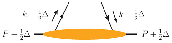
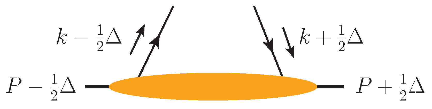
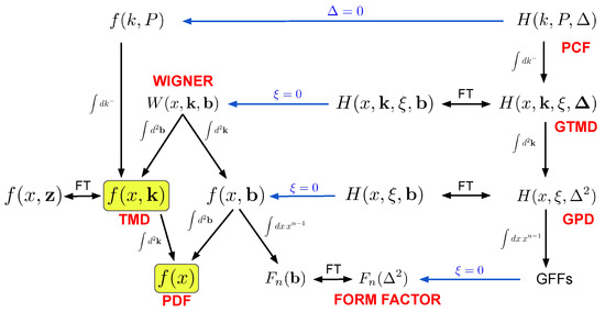
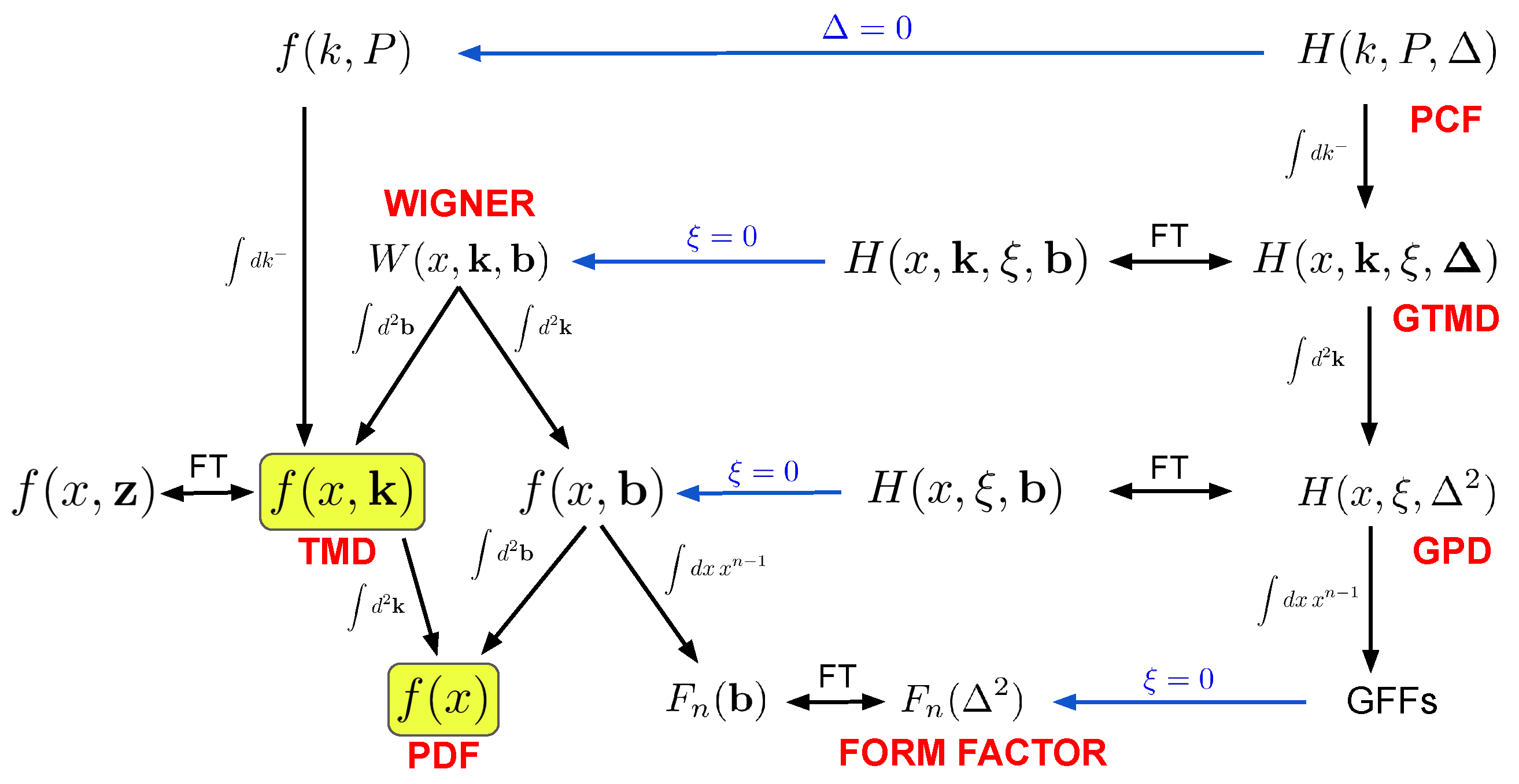
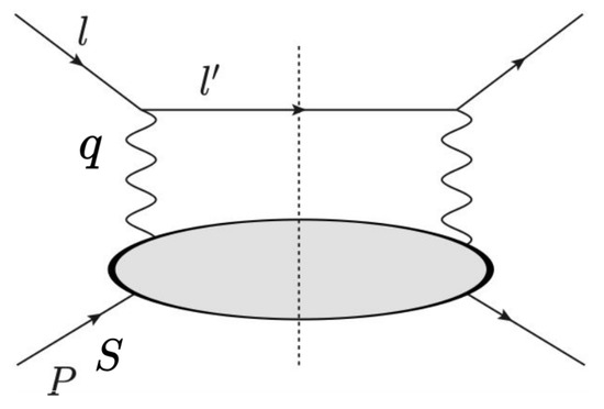
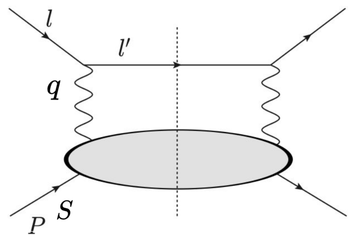


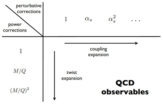
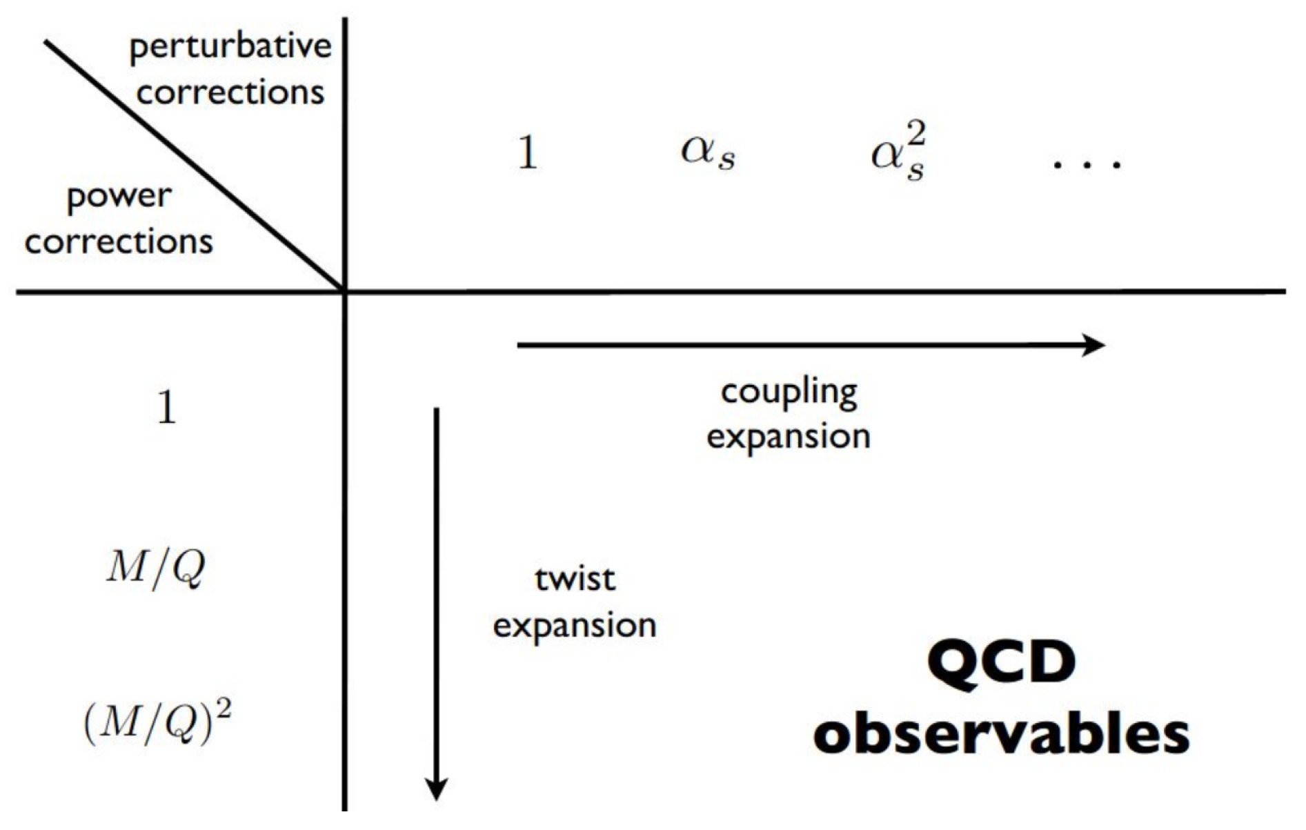
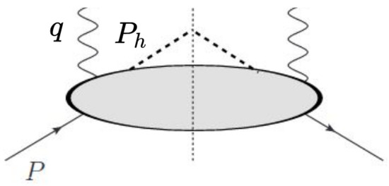
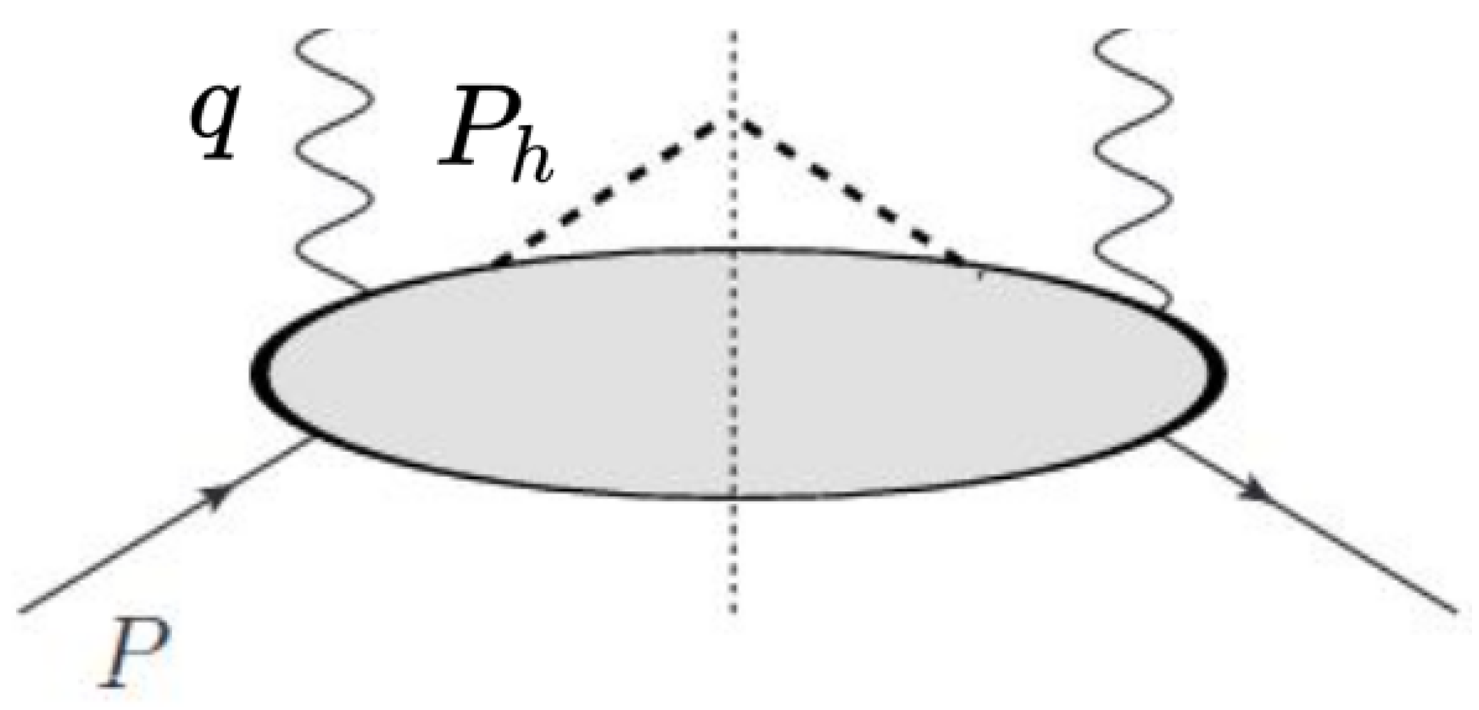
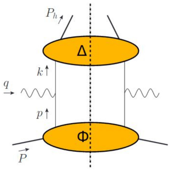
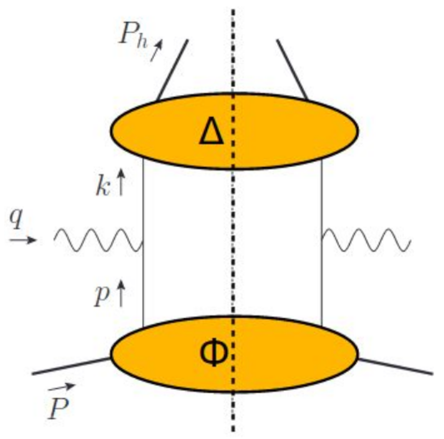
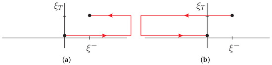

Disclaimer/Publisher’s Note: The statements, opinions and data contained in all publications are solely those of the individual author(s) and contributor(s) and not of MDPI and/or the editor(s). MDPI and/or the editor(s) disclaim responsibility for any injury to people or property resulting from any ideas, methods, instructions or products referred to in the content. |
© 2026 by the author. Licensee MDPI, Basel, Switzerland. This article is an open access article distributed under the terms and conditions of the Creative Commons Attribution (CC BY) license.