


Abstract
We review the role of primordial black holes (PBHs) for illuminating the dark ages of the cosmological evolution and as dark matter (DM) candidates. We elucidate the role of phase transitions for primordial black hole formation in the early Universe and focus our attention on the cosmological QCD phase transition within a recent microscopic model. We explore the impact of physics beyond the Standard Model (SM) on the cosmic equation of state and the probability distribution for the formation of PBHs, which serve as candidates for DM and contribute to present-day binary black hole merger events.
1. Introduction
The search for sub-solar mass mergers is of particular interest for cosmology and astrophysics, as such compact objects hint at new physics [1,2,3]. On 12 November 2025, the LVK collaboration reported a candidate sub-solar mass gravitational wave merger event [4,5]. This single candidate, if confirmed, could be direct evidence that primordial black holes (PBHs) populate the sub-solar mass window—a region inaccessible to standard stellar evolution and therefore a unique fingerprint of early Universe physics [6]. However, another interpretation of this event in terms of a subsolar mass neutron star merger has been discussed as well [7]. PBHs form in the radiation-dominated era when sufficiently large overdensities cross the particle horizon [8]. Unlike other relics, they carry direct information on the Universe before Big Bang Nucleosynthesis (BBN): their mass spectrum is a fossil of the cosmic equation of state (EoS) at their formation [9,10,11,12]. The PBH distribution from the thermal history is constrained by many observations [4,6,13,14,15,16]. Any modification of the thermal history therefore leaves a direct imprint on the PBH mass distribution and can mitigate the constraints.
The Big Bang scenario describes the early Universe as an extremely dense plasma of fundamental particles, cooling and expanding on a radiation-dominated background. As it cools, a succession of phase transitions (PT) occurs. It is of primary importance to map the nuclear matter phase diagram to understand how the Universe evolved through this period and what kind of PT remnants can be found in observations [17,18,19,20,21,22]. While the SM predicts smooth crossovers for both the QCD and electroweak (EW) transitions, the motivation for at least one strong first-order PT remains compelling: a strong first-order PT can leave imprints in the Stochastic Gravitational Wave Background (SGWB) through bubble nucleation [19,23], and its order has direct consequences for baryogenesis [24,25]. The Sakharov conditions [26] require CP violation, departure from thermal equilibrium, and baryon number violation—conditions that a first-order PT naturally satisfies. The smooth EW crossover suggested by the observed Higgs mass [27] seems to disfavor EW baryogenesis in the SM [28,29], yet the research on beyond-standard-model (BSM) mechanisms remains very active [30,31,32,33].
Asymmetries in the lepton sector could also be powering first-order transitions. Schwarz & Stuke [34] showed that an accurate description of the early Universe requires accounting for lepton flavor asymmetries, which generate cosmic trajectories in the QCD phase diagram. A large primordial lepton asymmetry of the Universe (LAU) can suppress sphaleron rates, reconciling a large LAU with the observed small baryon asymmetry (BAU) [35,36], and can trigger a first-order QCD transition with a distinct SGWB signature [37,38,39]. Crucially, large lepton asymmetries before BBN are observationally allowed, as neutrino flavor oscillations starting at relax them to values consistent with CMB and BBN constraints [40,41]. Bödeker et al. demonstrated that these asymmetries reshape the PBH spectrum in a way potentially consistent with LVK observations [42].
In this work we extend this framework using a microscopic QCD model [43], incorporating BAU and LAU through state of the art Taylor-expanded susceptibilities up to 4th order, following [44]. We compute cosmic trajectories and the EoS across a range of baryon and lepton asymmetry scenarios and translate the results into PBH mass distributions, discussing their implications for gravitational wave and microlensing observations.
2. The Thermal History After the Big Bang
In this section, we develop the cosmic EoS across different transitions. We start by presenting the standard model picture, before discussing effects of Beyond-SM physics.
2.1. The Standard Model
The cosmological equation of state is described through SM interactions, assuming that the laws of physics are rigorously the same as those observed on Earth at present time. The Big Bang scenario describes the early Universe as an extremely dense plasma of fundamental particles in thermal equilibrium on an expanding background. The rate of particle interactions being much larger than the Hubble expansion rate [45], the primordial plasma can be described solely through thermodynamic equilibrium. In its early stage, the “cosmic soup” is radiation-dominated (This study focuses on the radiation-dominated era; later times or the early matter-dominated era are outside the scope of the current study.) and cools down with time according to [46]:
where is the effective number of relativistic degrees of freedom for the energy density and . As it cools down, transitions to different phases of matter occur; let us make a brief summary. After the Planck time corresponding to a temperature , when all four fundamental interactions are unified, the Universe is minuscule, and quantum fluctuations are non-negligible. After , gravity decouples and the Grand Unification Era begins. It lasts until the strong interaction decouples at s with , which triggers the inflation era. According to Guth’s inflationary scenario [47], if the Universe undergoes a first-order phase transition with sufficient supercooling during this early epoch, it can enter a period of exponential expansion driven by the energy density of a false vacuum state. This inflationary phase addresses two fundamental problems of the standard Big Bang model: the horizon problem and the flatness problem. The exponential expansion during inflation stretches quantum fluctuations, filling the Universe with patches of inhomogeneity in energy density and curvature.
The decay of the inflation field marks the start of the quark-gluon plasma (QGP) phase. The deconfined quarks and ambient gluons provide the bulk of the contribution to the thermodynamics until the temperature drops down to [48], when a smooth crossover to the hadron resonance gas (HRG) occurs as quarks get confined into hadrons that (except protons) subsequently decay. Such energy regimes can be explored experimentally through large-scale projects such as the LHC [18]. In heavy ion collisions, the fireball formed can be similar to the very early Universe in terms of temperature regime, but it is significantly different when looking at the baryon’s net number density and chemical potential. Also, the lifetime of the experimental fireball is much smaller than the Big Bang time scale. Therefore, one cannot straightforwardly apply LHC results to the Big Bang model. It is of primary importance to properly map the QCD phase diagram for cosmology and particle physics experiments; see [20,21] for a recent overview. The preferred way to explore the nuclear matter phase diagram in the Big Bang regime is through lattice QCD simulations. In this study, we rather use the generalized Beth–Uhlenbeck (GBU) approach to the EOS of strongly interacting matter, which we will refer to as the microscopical model.
According to the GBU approach, hadrons appear as correlations in the strong interaction among quarks, which are described by phase shifts with a characteristic jump by for a bound state and a smooth tail describing the continuum of scattering states. These phase shifts in different hadronic channels are subject to in-medium modifications such as the chiral symmetry restoration (SR) and bound state dissociation (Mott effect). When one reverses the cosmic evolution so that the temperature increases and passes , the chiral condensate melts, and the quark masses drop toward their current-quark mass values in the SR crossover transition. As a consequence, the continuum edges for two-, three-, and multiquark states are dramatically lowered and “eat up” the hadronic bound states, which, upon further temperature increases, disappear as fading resonances in the continuum of few-quark scattering states. At the same time, when the quarks lose most of their mass upon SR, they appear as dominant degrees of freedom together with the gluons, which are set free by the simultaneous breaking of the center symmetry of the SU(3) color charge of QCD. This aspect of the QCD transition is captured in the behavior of the traced Polyakov loop and its potential. With the emergence of deconfined quarks and gluons in their QGP state, perturbative quark-gluon scattering processes also play an important role and have been included in the microscopic model, which provides an excellent description of QCD thermodynamics in accordance with ab initio lattice QCD simulations. For a detailed description and further results of the approach, see [43]. An advantage of the microscopic approach over that of the lattice QCD simulation is its flexibility when applications to cosmology are considered. We can straightforwardly extend the temperature range of the calculation, add photons, leptons, further quark flavors and hadron species, as well as extend the application to nonzero chemical potentials of baryon number and different flavors.
Once the pressure P as thermodynamic potential of the grand canonical ensemble is known, thermodynamic relations can be used to obtain the entropy density s, the number densities and the energy density :
where the temperature T and the set of chemical potentials are the free parameters characterizing the thermodynamic state of the system. The thermal equilibrium allows us to write any summable thermodynamic quantity marked with X as
where the subscripts and their corresponding particle species are self-explanatory. The QCD sector encapsulates deconfined quark and gluon interactions. denotes the number of quark flavors considered; our base data from the microscopic model contains quarks. Conveniently, at the QCD transition, heavier quarks have almost fully vanished. Recent studies show that heavy charmed hadrons/mesons are formed at the QCD transition [49,50]. However, since the charm quark abundance is already negligible at this temperature scale, the added contribution to the total thermodynamics is negligible. For consistency, we still added the data found in [50] to the mix, without any significant effect, as expected. Every particle mass was set according to [27]. In higher-temperature regimes, the inclusion of heavy quarks is required for a realistic picture. It is tempting to straightforwardly add a gas of free quarks to the mix on the grounds that the QCD sector at these temperatures is already very close to an ideal gas of free quarks; however, such an approach cannot account for the interaction between the heavy quarks and the gluons. At tree level, we can evaluate the (2+1+1) configuration with (2+1) as follows (from Supplementary Information of [17]):
where is the Stefan–Boltzmann limit for quark flavors considered, and is the pressure of a gas of free quarks. Note that the Stefan–Boltzmann limit should not only take into account quarks but also gluons, i.e., a non-interacting gas of massive quarks and eight massless gluons. A similar treatment to that shown in Equation (6) can be applied to extend the description of the QCD sector by adding bottom and top quarks (see Appendix A).
Between the start and decay of the QGP phase lies another transition: at –, the electromagnetic and weak interactions split, referred to as the electroweak phase transition (EWPT). The Higgs vacuum expectation value v is also set at this time; the observed mass of the Higgs boson is thought to be high enough to produce a smooth crossover rather than a proper phase transition per se [28,29]. In other words, v evolves continuously from the symmetric phase to the broken symmetry phase with . In the symmetric phase, the cosmic soup is effectively a mix of massless particles. Such a smooth crossover prevents the formation of cosmological relics like domain walls or cosmic strings, which can leave distinct imprints in the SGWB [23]; see [19] for a review.
Phase transitions, whether first- or second-order or a crossover, leave distinct imprints in the EoS. A deviation from the pure radiation value occurs there, see Figure 1. Here, we corrected the thermodynamics up to the bottom quarks. Given the mass of the top quark and the fact that quarks heavier than the strange do not significantly contribute to the QCD transition, ignoring their contribution in the microscopical temperature range [1:1300] is realistic. We see that the QCD transition is the most prominent feature of the EoS in Figure 1. At the confinement of quarks into hadrons and mesons, the entropy and energy density drop, as well as the pressure, though less steeply, creating a dip in the EoS parameter w. The same parameter rises to the radiation value after the transition as the leptons and photons become the dominant source of pressure. Then, another dip appears at , corresponding to the annihilation of the newly formed pions.
Figure 1.
Cosmic EoS tree-level corrected up to the bottom quark, Equation (6), for the SM (blue) and SM+X17 case (red). For , at the EWPT scale, we used data from Laine & Meyer [51]. For , we used the NUDEC BSM code [52,53] to model decoupling. Dashed vertical lines denote key temperatures.
Once the QGP has vanished, the other species contributions start to be significant; see Figure 2. Neutrinos and photons are added as a relativistic ideal gas of massless fermions and bosons. For charged leptons, we use a non-degenerate ideal gas of massive particles approximating the Fermi–Dirac integral with Bessel functions; see Appendix of [12] for details. The bump in lepton contributions just after the QCD transition in Figure 2 is due to the muons, which have not yet annihilated. Their mass of is close to the critical QCD temperature , so that when the QGP has almost fully decayed, the charged lepton gas is the main pressure contribution for a short time. Then, the muons decay and the charged lepton pressure drops, carried from this point on only by electrons.
Figure 2.
Partial thermodynamic contributions from different particle species and flavors in the standard case “Std b, std ℓ”. While the model introduces asymmetries, their small values () make it effectively identical to the blue curve shown in Figure 1. The red shaded region highlights the QCD transition pseudo-critical temperature . The different species contributions can be read in the legend; “B” denotes bosons. All of the neutrinos contributions, with dotted lines, are the same and the lines overlap.
At , the neutrinos start oscillating, the individual lepton flavor asymmetries mix with each other according to the mixing angle [40], and are fully decoupled at . Eventually, the electron contribution starts to vanish as electrons annihilate with the positrons at , heating up the cosmic components still coupled with photons, mainly hadrons. This succession of processes also leaves a signature in the EoS parameter, modeled here using the publicly available code NUDEC BSM [52,53].
2.2. Beyond the Standard Model
In the previous section, we described the Universe in its most standard way. The picture is consistent with (most) particle physics observations but does not address some fundamental cosmological conundrums. Unknown or overlooked BSM physics could be the culprit. Let us start from the most grounded observations by mentioning “anomalies” in the SM. Experimental research on BSM physics is a particularly active field; so far, many “anomalies” (most often in the form of resonances) have been found in nuclear and particle physics experiments. The extension in particle physics can occur in the sectors of fermions (spin 1/2), scalar bosons (spin 0), and vector bosons (spin 1). For a recent overview of anomalies in particle physics, see Crivellin & Mellado [54]. In a previous study, we looked at the impact of the putative X17 boson [55,56] on the cosmic EoS and the PBH distribution around the QCD transition, see [12]. In Figure 1, we updated the previous study by including annihilation and the standard crossover at the EW scale. This picture remains close to the standard case, as we do not include new physics per se, but simply add another non-interacting boson to the thermodynamics. It acts as a proof of principle of how particle physics “anomalies” can leave a cosmological imprint.
Turning now to cosmic mysteries, we already mentioned the need for a baryogenesis mechanism able to match the observed baryon asymmetry inferred from Planck [57]. In the SM, b is supposedly linked to the lepton asymmetry ℓ through the Sphaleron process, allowing violation of baryon B and lepton L numbers while conserving . We are not concerned here with the underlying mechanism leading to baryo- or leptogenesis; we refer the interested reader to the reviews and references therein [24,25]. Nevertheless, we want to examine the thermodynamic impact of an asymmetric Universe in baryon and lepton number, i.e., accounting for chemical potentials —respectively, the baryonic, electric charge, electronic, muonic, and tauonic sectors. Efficient sphaleron processes would yield ℓ = −51/28 × b [58]. Such a scenario would remain very close to the picture described in Section 2.1 and the blue curve of Figure 1, as the asymmetries b and ℓ are very small and the induced chemical potentials do not significantly impact the thermodynamics. It was pointed out in Ref. [34] that an accurate description of the early Universe requires accounting for those asymmetries, as their introduction along with conservation of the associated charges (see Equations (7)–(9) below) generates cosmic trajectories in the QCD phase diagram; see Section 4,
where is the net baryon number density, is the net charge number density, is the net lepton number density, ℓα is the lepton flavor asymmetry for the flavor , and s is the total entropy density from Equation (5). We stress that all the number densities are net: , and similarly for the neutrinos.
Many ideas and BSM processes have been proposed to generate a baryon asymmetry, often able to generate values above observations. For instance, the Affleck–Dine (AD) mechanism assumes the possibility of inhomogeneous baryogenesis, i.e., there could be patches of the Universe with a high baryon number [59,60]. The AD mechanism also predicts the possibility of a globally high baryon number, which could trigger a 1-order QCD transition. Understanding how the PT occurs in these regimes is necessary, as unexpected processes could evade the constraints on the baryon asymmetry. Boeckel & Schaffner–Bielich suggested a “little inflation” era (or supercooling) at the QCD crossing for followed by reheating [30,31]. We want to study how these models could evolve thermodynamically, and to do so, we use QCD thermodynamics with from [43].
Another pathway for an early Universe with high baryon chemical potential, which does not require a large baryon asymmetry, is through lepton flavor asymmetries, which recent analyses find to be up to [61,62,63,64,65]. The AD mechanism could also be the culprit for such a value of the LAU [66]. The idea is straightforward: large values of lepton asymmetries before BBN are hard to constrain, as neutrino oscillations starting at can change the lepton flavor asymmetries to values fulfilling the constraints [40]. Some values of lepton flavor asymmetries are preferred by CMB and BBN [41,67]. It should be noted that in the references above only neutrino chemical potentials are taken into account in the calculations, i.e neutrinos only carries the asymmetries. The present calculations, based on Equation (7), distribute the asymmetry between both charged leptons and neutrinos, resulting in non-vanishing chemical potentials for the former; their contributions are subdominant at , which makes the CMB and BBN constraints still relevant, even though not exact. Only a direct measurement of the infamously hard-to-measure Cosmic Neutrino Background could shed light on the MeV era. None of the models presented in this study are favored by neutrino oscillations; the aim of the present paper is to examine how the LAU affects the thermal history and to link it to PBH formation in the manner of Bödeker et al. [42]. An exhaustive study of the preferred LAU configuration is planned.
3. Methods
After presenting the thermal history after the Big Bang in various contexts, we now turn to how to solve the conservation equations. In order to solve Equations (7)–(9), the dependence of the entropy density on the baryonic and electric charge chemical potentials must be evaluated. To do so, following the procedure introduced in Refs. [34,44,68,69], we rely on a Taylor expansion over the tree-level correction up to the charm quark. We used state-of-the-art QCD pressure derivatives, called susceptibilities, up to 4 order from [50,70]. The lepton sector was solved using the Fermi-Dirac integrals with the JEL approximation [71]. Even though our approach is very similar to the latest study [44] and we used the same susceptibilities for the Taylor expansion, our base entropy density does not come from lattice QCD calculations but rather from the microscopic model [43]. This comes with the advantage of continuous trajectories, rather than 3 distinct regimes. We also extended the calculations to higher temperatures using polynomial extrapolations from Bresciani et al. [72] and interpolation from to . The interpolation range is chosen for a smooth connection between the two data sets; see Appendix A.
The (2+1) susceptibilities from Ref. [70] range from [30:800] ; we used the Thermal-Fist package [73] for computations below . In order to properly include the charm quark in the calculation, we also need the (2+1+1) susceptibilities. Using the susceptibilities from [50], one can derive the relevant susceptibilities , , including the charm quarks. We also extrapolate the susceptibilities from Refs. [50,70] to high temperatures. It can be seen in the figures of the mentioned references that the susceptibilities tend to tend to ∼95–90% of the SB limit at asymptotic temperature. We added a point at 90% of their SB limit at and performed a polynomial fit to ultimately extend the Taylor expansion to higher regimes. We set the extrapolation limits at 90% of their SB values, since lattice QCD results [72,74] suggest that QCD matter thermodynamics tends to ∼90–85% of the SB limit at high temperatures. It has been demonstrated in Ref. [43] that the correction to the ideal gas pressure due to quark–quark interaction via one-gluon exchange leads precisely to this reduction in the SB limit. The tree-level evaluation of the charm and bottom quarks conserves this behavior at the limit; see Appendix A. We show as an example in Figure 3. We observe a similar behavior for the (2+1) and (2+1+1) cases, the former being a reliable pure lattice QCD calculation; the similarities between the red and blue curves show that the inclusion of the charm quark and the polynomial extrapolation are fairly reliable. The comparison with the model of an ideal gas of massive quarks and massless gluons shows how poorly this approximation describes the QCD transition. We stress that the absence of susceptibility data including heavy quarks at high temperature is one caveat of our approach. The present study should motivate the further exploration of this temperature regime.
Figure 3.
comparison between the ideal QCD sector comprising massive quarks up to the charm sector and gluons, shown as the black dashed line; the data from Ref. [70] in red; and the derived inclusion of the charm quark using Ref. [50] as blue dots. The SB limits are shown as colored squares to the right of the plot.
4. Results and Discussion
4.1. Equation of State with LAU and BAU
After having presented the equations to be solved in Section 2 and how we extended the analysis in Section 3, we now look in detail at the resulting EoS and trajectories of cosmic evolution.
The LAU triggers an increase in the absolute value of the lepton chemical potentials. Then, electric charge neutrality, Equation (9), imposes a correlation between the QCD net electric charge and the lepton sector net electric charge . It follows that the chemical potentials associated with the quarks also increase in absolute value. We can see how the LAU changes the cosmic trajectories in the nuclear matter phase diagram in Figure 4. The dashed gray and black lines correspond to models presented in Bödeker et al. [42]. The dashed red line, also presented in the same study, corresponds to the case with lepton asymmetry associated with the sphaleron process , which we call the standard case “Std b, std ℓ”. The dash-dotted line corresponds to an extreme scenario where and the Taylor expansion is no longer reliable. For this dash-dotted model, we only present the massive non-interacting quark and gluon gas approximation. For easier comparison with the other models, the charm quark is the most massive quark of the model. The quarks and leptons have associated chemical potentials:
where is the electric charge chemical potential, (also written ) corresponds to the neutrino flavor chemical potential and represents the charged leptons. The gluons are treated without chemical potential as an ultra-relativistic gas of massless bosons. All the dashed lines in the figures throughout this study are determined for from [57], consistent with constraints on the electric charge of the Universe [75], and arbitrarily fixed, corresponding to realistic trajectories found by solving the conservation equations Equations (7)–(9).
Figure 4.
Cosmic trajectories for different scenarios: the dashed lines correspond to realistic scenarios. Colored dots show the trajectories with const imposed. The purple dash-dotted line marked as “High b IG” corresponds to an ideal gas (IG) calculation with ; the lime green dashed line marked as “Std b, high ℓ” corresponds to ; the black dashed line marked as “Bödeker-like 1 path”: ; the gray dashed line marked as “Bödeker-like 2 path”: ; the red dashed line marked as “Std b, std ℓ”: . See Appendix B for the cosmic trajectories in the T vs. planes. The parametrization of (red dotted) is taken from [76].
Since the Taylor expansion breaks down when , the extreme dashed-dotted model is computed only at high temperatures using the ideal gas approximation. Furthermore, a pion condensate can form when or , which could leave an imprint in the SGWB [77,78,79,80]. The entry into and departure from the condensate could be a 1 or 2 order PT depending on the value of . We show the pion mass in the T vs. plane in the Appendix B Figure A2. None of the realistic trajectories presented form a pion condensate. The cases with const also do not form a pion condensate because in the microscopic model.
Gao & Oldengott [37] used a functional QCD method to explore cosmic trajectories with high lepton flavor asymmetry. They find the signature of a 1-order QCD transition when looking at the quark chemical potential [22,37,39]. The condition for a 1-order PT relies on the determination of the critical end point (CEP), where the PT stops being a crossover. They find that if MeV at the PT is 1-order. None of the realistic cosmic trajectories fulfill this condition.
While it is clear that paths with const are not realistic around the QCD transition, they remain interesting when considering AD baryogenesis or high lepton flavor asymmetries. Such trajectories could approximate the thermodynamic evolution of the models proposed by Boeckel & Schaffner-Bielich [30,31] or the High Baryon Bubbles proposed in [60]. These regions could retain a high baryon number and somehow evolve independently if they are large enough, i.e., on superhorizon scales. We want to keep the number of assumptions to a minimum, so that we do not include lepton asymmetry in the calculations of these models; we take the data from Figures 8 and 12 of [43] and insert them in Equation (5). The paths with const use (2 + 1) quark flavors, while the dashed lines use a tree-level correction to account for the charm quark as well. The reason lies in Equation (6). The accurate determination of in the presence of chemical potentials would have to take into account the electric charge chemical potential; see Equations (10)–(12). Since depends on the lepton asymmetry and we chose to use a simplistic model, we shall remain conservative and not add any tree-level corrections. The charm quark is not thought to be very significant at the QCD transition [12,50]; the leptons, however, are, and with fixed, we do not compute the lepton chemical potentials—we discuss the effect of this choice in the following paragraphs. A “zig-zag” feature can be seen at for the case . The parameters of the microscopical model were tuned to unify the QGP and HRG phases at , where the lattice QCD is the most reliable. With non-vanishing , a discontinuity appears because the microscopic model treats the hadrons and quarks distinctly with a sharp cutoff at . Increasing makes the discontinuity more significant, as seen in [43].
It is worth noting that at , the slopes of the paths with const are similar to those of the “High b IG” and “Std B, high ℓ” models. This is because, with massless particles, which is a reasonable approximation away from the QCD transition, the charge conservation Equations (8) and (9) are analogous to const. In the Appendix of [44], they find valid for .
The EoS of the different models is plotted in Figure 5. The dashed gray, black and red lines reproduce the Bödeker results; the dip in the EoS at the QCD transition is mitigated by the baryon chemical potential but also by the lepton chemical potentials. It is clear from the colored continuous lines that the baryon chemical potential does provide a mitigation of the softening, but the difference with the “lepton powered models” shows that the lepton sector might be even more important when it comes to creating a shallower dip at the QCD transition. We explain this through the muon lepton: in the two Bödeker-like and “Std b, high ℓ”, is large; hence, follows, which makes the contribution of the muon sector more significant; see Figure 6. At , the muons have not yet decayed and can therefore still compensate for the dip created by the QCD transition.
Figure 5.
EoS corresponding to the different cosmic trajectories. The same color code from Figure 4 is applied. Between and , the thermodynamic quantities have been interpolated. Since no physics processes are modeled in this intermediate region, the equation of state parameter remains constant for the case . The same interpolation method is applied to both the energy density and pressure P; consequently, w remains constant across all trajectories. For non-vanishing , the Taylor expansion makes the stalling of w less significant.
Figure 6.
Partial thermodynamic contributions from different particle species and flavors in the case “Std b, high ℓ” with high lepton flavor asymmetries. .
In Figure 6, the effect of high on the contribution is clear. Looking closely at the purple lines, we see how the decay of the charged leptons is associated with the rise of the as the “ leptonic” charge must be conserved. Comparing with Figure 2, we see that the QCD sector does not necessarily dominate the pressure or energy density at high T in the presence of LAU. Furthermore, the behavior of the different species contributions is not identical between different thermodynamic quantities. In “Std b, std ℓ”, charged leptons dominate shortly after the QCD transition; with the “Std b high ℓ” model, neutrinos are the dominant contributors to the entropy density after the QCD transition. The charged leptons might come close to the neutrino contribution, but the decay of the muon, associated with a rise in contribution, leaves the charged lepton contributions subdominant. For the same model, there is a sharp drop in entropy and energy density at the QCD transition, corresponding to the zig-zag in the associated cosmic trajectory Figure 4.
Increasing also comes with the effect of shifting the minimum of the softening to lower temperatures; this is not observed in the presence of lepton asymmetry because is small. The effect is not very significant, but it can be explained by the well-known shift of to a lower value as increases [48,76], shown in Figure 4 as the red dotted line. is close to the standard case, and the minimum is barely distinguishable. The dip to the minimum is steeper compared to the Bödeker-like and standard models, which can be partially explained by the difference in the number of quark flavors; see Figure 2 from [12]. The inclusion of heavier quarks would make the rise to slower, because massive quarks such as the bottom are not yet ultra-relativistic.
One more notable feature of the continuous colored lines appears at high temperature: w rises above the radiation value, corresponding to a Universe “stiffer” than what can be expected with pure radiation. Such an effect is not observed in the Bödeker-like models, because the baryon chemical potentials are not high enough for departures from pure radiation at high temperatures. The purple dash-dotted line, where the QCD sector is an ideal gas of massive quarks and gluons, also sits around at high temperature; even though it has a large chemical potential, the Fermi–Dirac distribution imposes in any case. The lime green dashed model also shows at high temperatures, which can be explained by the fact that this model also exhibits high chemical potential at high temperatures, triggering the departure from the ideal gas.
Since w is simply defined as the ratio of pressure over energy density, is not a limit indicating incorrect physics. In Figure 7, we plot the pressures of the different models and their associated IG approximations, which act as upper limits. It is clear that all the models sit below the IG limits. The behavior of the energy density is similar. The purple “High b IG” shows the highest pressure, as it is also the model with the highest chemical potential. It might be surprising not to find the fixed models on top of the others, but we are plotting the total pressure from Equation (5), and these models do not account for lepton chemical potential; hence they might not even exhibit higher pressure values than the “Std b, std ℓ” model. This shows how important it is to take into account the conservation equations Equations (7)–(9).
Figure 7.
Normalized pressures , the same color code from Figure 4 is applied. The dashed-dotted lines correspond to the ideal gas cases. The slight discontinuity in “Std b, high ℓ” around T = 30–40 correspond to the concatenation of the microscopical model with Thermal-Fist [73].
Having established the cosmic trajectories and their thermodynamic consequences, we now turn to the PBH mass distributions induced by the different LAU.
4.2. The Primordial Black Hole Mass Spectrum
In this section, we briefly reintroduce the formalism to translate the EoS into a PBH distribution. For a detailed discussion, see [10,11,12] and the references cited in the following paragraph. Primordial black holes are a unique probe of the early Universe; since these objects form in the radiation era, they can provide a picture of the Universe before the CMB. Notably, this was proposed as a probe for lepton flavor asymmetry in [42]. We argue here for a similar idea, computing the PBH mass spectrum from the EoS presented in Section 2 and comparing the induced distributions and their implications for future observations. Fluctuations of energy density in the very early Universe are necessary to explain the current energy distribution of the Universe. Hawking and Carr introduced the idea that some of these early fluctuations could have been large enough to collapse to PBHs when the particle horizon crosses the fluctuation radius at [8]. Although early energy density fluctuations may have many possible origins, the main scenario is cosmic inflation, which typically assumes a Gaussian fluctuation spectrum. No matter what the source of the fluctuations is, they should be larger than the Jeans length at maximum expansion if they are to undergo gravitational collapse. Recently, Carr explored different formation scenarios [13,14], and various studies provide numerical simulations of the collapse of overdensities [11,81,82,83,84]. We refer interested readers to the 2021 review by Escrivà [85] and the references therein. These studies find that a PBH does not form exactly at the horizon mass, which has the notable effect of widening peaks in the distributions; the QCD peak, for instance, sees its width increase. For simplicity, we stay in the purely analytical formulation, as we are interested in drawing a general picture of the PBH spectrum. Collapse can occur at different epochs during the radiation-dominated era, depending on the size of the fluctuation. From Equation 2.2 of Ref. [86], the particle horizon grows as follows:
where is the number of degrees of freedom of the energy density , is the mass in the cosmic horizon , accounts for the critical behavior of a collapse to a PBH, i.e., reflecting the fact that PBHs are not born with exactly . (Note that Equation 2.2 from Ref. [86] seems to partially incorporate the critical behavior of a PBH collapse. The Choptuik’s critical collapse law [87,88] appears more complex. Nevertheless, the equation from Ref. [86] is standard in PBH studies, as similar ones are presented in Bödeker et al. [42] or Carr et al. [15].) For simplicity and because we are mainly interested in describing tendencies, we set . From Equation (13) , so that a change in the value of would slightly shift the peaks to lower masses; see [86], where they use . The introduction of the factor is simplistic, as it is often set as a constant independent of temperature. In fact, one would expect to change as the matter changes phase and to depend on the actual energy content; for instance, when comparing Figure 2 and Figure 6, we see how the presence of high LAU changes the energy density and pressure content drastically. One should expect the physics inside an overdensity to be different for a Universe whose energy density is dominated by leptons compared to a QCD-dominated one.
In the past five years, new developments have emerged; different statistical methods now exist to evaluate the PBH mass spectrum through compaction function [81,89] or peak theory [90,91]. The evaluation presented here does not compete with these approaches and represents a less accurate representation of the PBH mass spectrum from the thermal history. Nevertheless, regardless of the method used, the overall impact of phase transitions on the PBH spectra is the same.
The size of candidate PBH fluctuations increases with time; a full PBH mass spectrum is possible from Planck’s mass ( g) if formed at Planck’s time ( s) to the supermassive range () for those formed as late as 1 s after the Big Bang [14]. It should be noted that Equation (13) depends on , which is a thermodynamic function, so the horizon mass differs slightly between the different models. For a detailed comparison between the SM and SM+X17 scenarios, see the Appendix of [12]. We follow Carr’s prescription to fully describe an overdense region by its energy density contrast:
where is the energy density in the region, and is the background energy density. Then, the fate of an overdensity is determined by the relation between and the threshold [9]. If at , a PBH is formed; if not, the overdensity is eventually dispersed away by the pressure. Assuming Gaussian fluctuations, the fraction of the Universe collapsing is
where M is the PBH mass, is the complementary error function and is the root mean square amplitude of the Gaussian fluctuation; is taken from [83]. Following [15,42],
where is the spectral index taken at its CMB value [57]. On PBH scales, there is actually more liberty on the shape of and the value of ; for instance, could be running [86]. The amplitude A is a normalization parameter that expresses the strength of the fluctuations.
The present fraction of DM in a PBH of mass M is then
where is the horizon mass at matter–radiation equality. The numerical factor originates from , with and being the baryon and CDM density parameters from [57].
The dips in the EoS are of particular interest for PBH formation, as they can be understood as a softening of the Universe: they increase the chance that a given overdense region collapses into a PBH. In Figure 8, we show the PBH mass spectrum for the SM and SM+X17, including now the super-massive black hole (SMBH) production at annihilation, as well as the sub-solar peak at the EWPT. The logarithmic scaling can be deceiving as the SM+X17 seems to produce many more PBHs outside of the QCD peak. The slight mitigation of the QCD softening from X17 does not drastically modify the mass spectrum, but it does show an impact on the entire PBH spectrum. Although we do not show the PBH spectrum for fixed—since the absence of lepton chemical potential makes the behavior of the QCD transition unreliable—we can predict that the QCD peak would be mitigated, with the rest of the distribution increasing its contribution accordingly. The case would not be as straightforward, since indicates a stiff EoS prior to the QCD transition; production in this era would be harder, and PBH production would be mitigated. The increased production post-QCD transition seen for SM+X17, “Bödeker-like” and “Std b, high ℓ”, could have significant observational effects; we discuss this mass range extensively in [12] Sections 3 and 4.
Figure 8.
Comparison of SM and SM+X17 PBH mass spectra without chemical potentials. The legend gives , the fraction of DM in PBHs, and A, the normalization amplitude of . The asterisks denote the maximum of the distribution; the color code of the vertical lines is the same as in the Figure 1. Note that the vertical lines corresponding horizon mass and for the SM (dashed) and SM+X17 (dotted) nearly perfectly overlaps.
The standard case, Bödeker-like models and “Std b, high ℓ” are shown in Figure 9. In Figure 3 of Bödeker et al. [42], similar spectra are plotted, but the normalization of is not consistent between the models. Here, we plot them again with . Again, the mitigation of the QCD peak triggers increased production in other eras, similarly to the SM+X17 case. “Std b, high ℓ” might be the most notable one, as it shifts the largest peak to a smaller mass. Looking at the right panel Figure 9, the region does not represent the bulk of the PBH population for “Std b, high ℓ”. The formation of a dome pre-QCD transition at is caused by the decay of the lepton, leaving a deep imprint in the thermal history; see Figure 6. For models carrying a large tau lepton chemical potential, annihilation helps to soften the EoS pre-QCD transition, but the onset of the contribution to carry mitigates the QCD drop and hence the production. The neutrinos dominate P and after the QCD transition, so the behavior of the EoS and PBH production comes from the leptonic sector. At , the annihilate and completely disappeared by , creating another peak at . The number density of increases, and the neutrinos become the dominant thermodynamic contribution.
Figure 9.
Bödeker-like PBH spectra, “Std b, std ℓ” and the “Std b, high ℓ”. Using the same color code as Figure 4, Figure 5 and Figure 7. The shaded region shows the observations of GWTC-4 [92], including the analysis from Ruiz-Rocha et al. [93] up to . The asterisks denote the maximum of the distribution.
As mentioned in Section 2, a pion condensate can form in the presence of high lepton asymmetry, with impact on the PBH distribution [78]. Furthermore, cosmological relics from first-order transitions could also collapse into PBHs or interact with them [94,95,96]. PBHs have also been proposed as a probe for a first-order EWPT [97].
4.3. Discussing the Constraints and Positive Evidence
After showing how the PBH mass spectrum is modified in the presence of LAU and BSM anomalies like X17, we discuss how these results compare with current observations. We should start by stating that the aim of the present paper is not to constrain the models presented, nor to make quantitative predictions for future observations. We are mainly interested in describing the EoS behavior around the QCD transition across a diverse variety of models. The PBH mass spectrum is another way to look at the consequences of modifications of the EoS, and would become a direct probe of the Universe pre-BBN should future observations confirm the existence of PBHs. For a thorough review of PBHs and their implications, see Ref. [4] from the LISA theory group, or more generally, the work of B. Carr [6,13].
The stiffening of the EoS pre-QCD transition associated with sub-solar mass PBH formation has implications for microlensing observations. Although it is hard to draw firm conclusions because different collaborations claim different results and constraints, it remains worth mentioning, as it is an active field of research. Moreover, the constraints rely on assumptions that are not fully secured. For instance, the spatial distribution of PBHs could have a significant impact on the constraints; see the recent review by Green [98]. Hawkins in Ref. [99] discussed how the galactic rotation curve can bias microlensing observations. The current discussion, in a nutshell, is as follows: in the late 1990s and early 2000s, the MACHO collaboration reported observations consistent with a significant fraction of the Milky Way halo being composed of sub-solar compact objects [100,101]. EROS [102] and OGLE [103,104] were not able to corroborate the results. Hawkins & Garcia-Bellido [105,106] showed how using the Milky Way rotation curve inferred by GAIA can mitigate the constraints from OGLE. To add to the debate, the Subaru telescope can also be used to search for microlensing events in Andromeda; in their 2017 analysis, they found strong constraints [107] on the mass range –. A 2026 analysis [108] mitigates this original claim, explicitly stating that it originated from a better treatment of the data. Another way to constrain this mass range is through PBH–star interactions [109,110].
The sub-solar mass range is particularly interesting: on 12 November 2025, the LVK collaboration reported a candidate sub-solar mass merger event [4,5]. It was quickly followed by an analysis finding the merger rate of such an event to be compatible with a slightly modified version of “Bödeker-like 2” (the spectrum they present is tilted compared to the one from this study and Bödeker’s, which typically appears when modifying the value of in Equation (16)) [6]; see also [16]. PBH formation and the peaks associated with thermal history can leave hints in the SGWB [86,111]. In a broader sense, primordial fluctuations are also sources of the SGWB with associated bounds on the fluctuation power spectrum [112,113]; see Ref. [114] for a review.
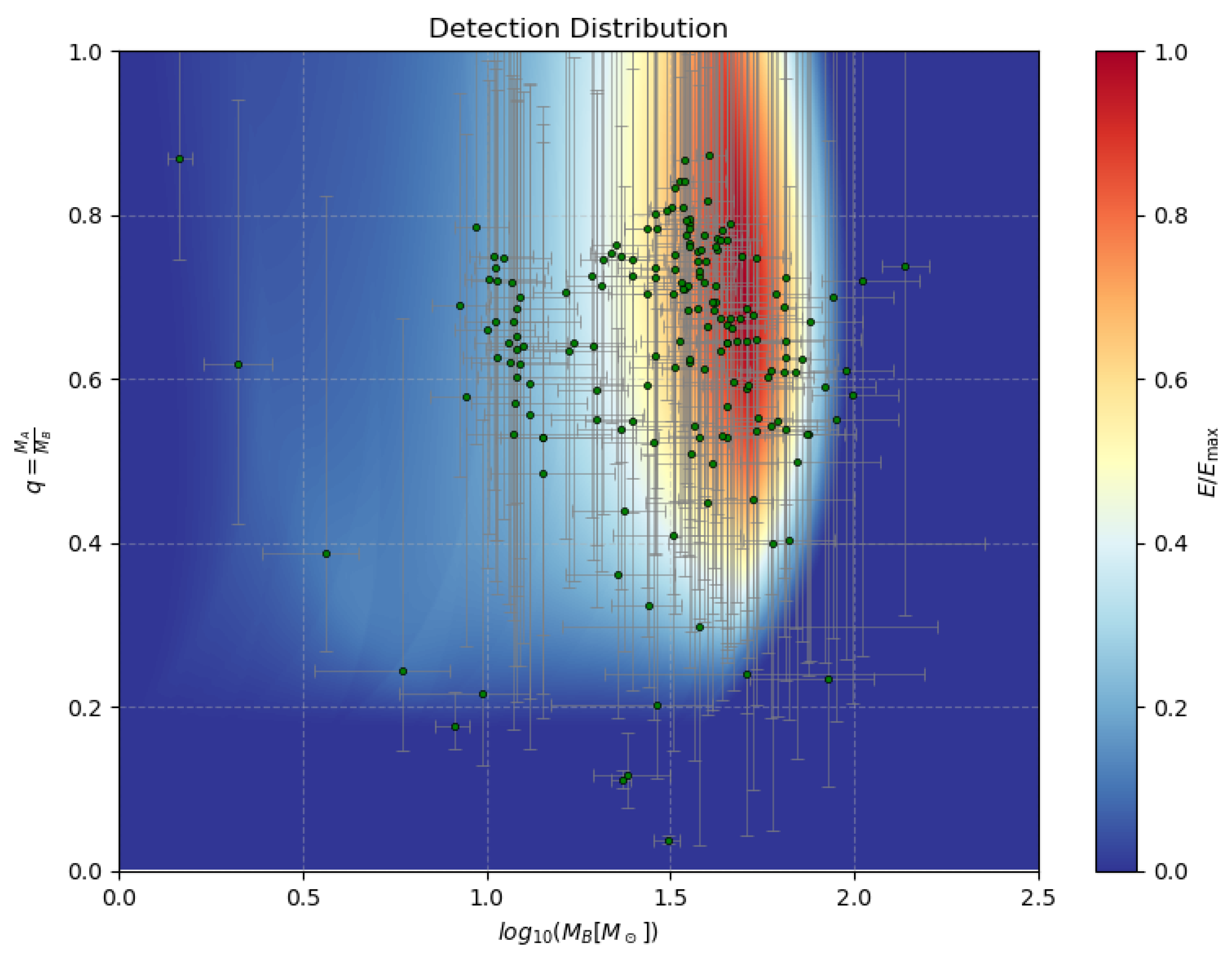
Stellar mass PBH production has direct implications for GW observations; see Refs. [4,5] for a recent review. As shown by Bödeker et al. in Ref. [42], lepton asymmetry can be a convenient way to make GW observations agree with the predicted PBH mass distribution from thermal history. We showed the current LVK observation mass range in Figure 8 and Figure 9. In Figure 10, we show how the probability density of PBH mergers compares to the actual events from GWTC-4 [92]; to model the PBH merger rate, we assume only late binaries [115]. Comparing with Figures 4–6 from Bödeker et al. [42], it is clear how the lepton asymmetry can shift the peak in the probability density of PBH mergers closer to the observed aggregate in the plane, where q is the mass ratio of the binary, and is the heaviest binary component.
On the more massive part of the spectrum, Ref. [116] showed that distortions (not related to muons nor chemical potentials) in the CMB power spectrum could draw limits on the higher portion of the PBH mass function. In the same intermediate BH mass range –, Ref. [117] constrains monochromatic PBH abundance through energy deposits in the CMB during the dark ages; see [118]. It is therefore crucial to include the LAU in the PBH mass spectrum estimates and so the SMBH peaks, as it could leave a distinct imprint on the SGWB detected by future experiments [4]. In the absence of a given signal, it would constrain the primordial fluctuations power spectrum, similarly to what is currently inferred from the CMB fluctuation spectrum, for instance. A quantitative study of the SGWB induced by the scenarios presented in this study is outside the scope of the article; we stress that such calculations are of primary importance to decipher the primordial parameters of the universe. On the other hand, it is tempting to understand the newly discovered population of supermassive black holes at high z, the “little red dots”, through PBH seeds [119,120,121]. Several mechanisms to form the little red dots from PBHs have been considered [122]; the massive seeds appear to be ruled out by -distortion, although the strength of the constraints depends on which statistical framework for PBH formation is adopted [113]. Moreover, supermassive PBHs could impact early structure formation through their seeding effect [123].
We close this section by stressing that the PBH mass spectra produced throughout this study are constrained by various observational channels. Although the results are difficult to compare directly with the extended mass functions, current observations are likely already ruling out the spectra presented in this study. We are particularly concerned with scalar-induced gravitational waves [113,114] and -distortion [116]. Nevertheless, our study shows that the relative abundance of different PBH masses can significantly change depending on the LAU, with implications for observations, as shown in Figure 10, which makes PBHs a compelling probe of the primordial Universe. We show that the characteristic peak from the QCD transition does not necessarily make up the bulk of the PBH population, as seen in “Std b, high ℓ” in Figure 9. The application of monochromatic constraints to an evenly distributed PBH mass spectrum is, to say the least, questionable.
Figure 10.
Probability density of PBH mergers with masses . Inspired by Figures 4–6 from Bödeker et al. [42]. Events from GWTC-4 are shown as green dots [92]. We used O4 strain noise from [124].
5. Conclusions
In this study, we explored the cosmic equation of state across the QCD transition for a range of baryon and lepton asymmetry scenarios, extending our previous work [12] to include non-vanishing chemical potentials and to show the complete thermal history in the presence of X17 bosons. Using a microscopic QCD model [43] combined with state-of-the-art lattice QCD susceptibilities up to fourth order [44], we computed cosmic trajectories in the nuclear matter phase diagram and their thermodynamic consequences over a temperature range up to by including charm quark corrections. We motivate the computation of susceptibilities of heavy quarks in a cosmological context. The extension to is also of crucial importance, as this epoch corresponds to the formation of SMBHs (see the last peak in Figure 8 or [15]). A future study accounting for LAU during neutrino decoupling is already planned.
Using two simplistic models with high baryonic chemical potential but without LAU, we clarified the role of the baryon and lepton chemical potentials on the thermodynamics, finding the possibility of a stiff universe pre-QCD transition that has not been considered so far. Furthermore, the comparison with realistic models highlights the importance of lepton asymmetry on the EoS. Unlike the previous Taylor expansion and lattice-QCD-based approaches, which rely on distinct hadronic, quark–gluon and non-interacting quark gas regimes, the microscopic model provides continuous trajectories across the transition, offering a smoother and more consistent description of the thermodynamics. We find that the baryon chemical potential alone does not capture the full picture of the primordial plasma at the QCD transition: lepton flavor asymmetries, through electric charge conservation, generate comparable or larger chemical potentials in the QCD sector and significantly mitigate the EoS softening. The resulting PBH mass distributions show distinct features—in particular, a pre-QCD stiffening and a modified QCD peak—that differ qualitatively from the standard scenario. The recent LVK sub-solar mass candidate [4,5] and its compatibility with lepton-asymmetry-driven PBH scenarios [6] motivate a deeper quantitative comparison, which we plan to address in a future study including a more systematic exploration of the lepton asymmetry parameter space and a tighter confrontation with gravitational wave observations.
Author Contributions
Conceptualization, M.G., G.H., D.B., O.I.; methodology, M.G.; software, M.G.; validation, G.H., D.B., O.I.; formal analysis, M.G.; investigation, M.G.; resources, M.G.; data curation, M.G., O.I.; writing—original draft preparation, M.G.; writing—review and editing, M.G., G.H., D.B., O.I.; visualization, M.G.; supervision, G.H., D.B., O.I.; project administration, M.G.; funding acquisition, G.H., D.B. All authors have read and agreed to the published version of the manuscript.
Funding
The research of D.B. and O.I. was part of project No. 2021/43/P/ST2/03319 co-funded by the National Science Centre and the European Union Framework Programme for Research and Innovation Horizon 2020 under Marie Skłodowska-Curie grant agreement No. 945339. For the purpose of Open Access, the author has applied a CC-BY public copyright license to any Author Accepted Manuscript (AAM) version arising from this submission.
Data Availability Statement
The data used in this study is available through the DOI: 10.14278/rodare.4776.
Acknowledgments
We thank Alberto Magaraggia for the code plotting Figure 10, Lorenzo Formaggio, Francesco Di Clemente, Dominik Schwarz, Julien Froustey, Albert Escrivá and Florian Kühnel for the fruitful discussions.
Conflicts of Interest
The authors claim no conflict of interest.
Appendix A. Base Thermodynamics
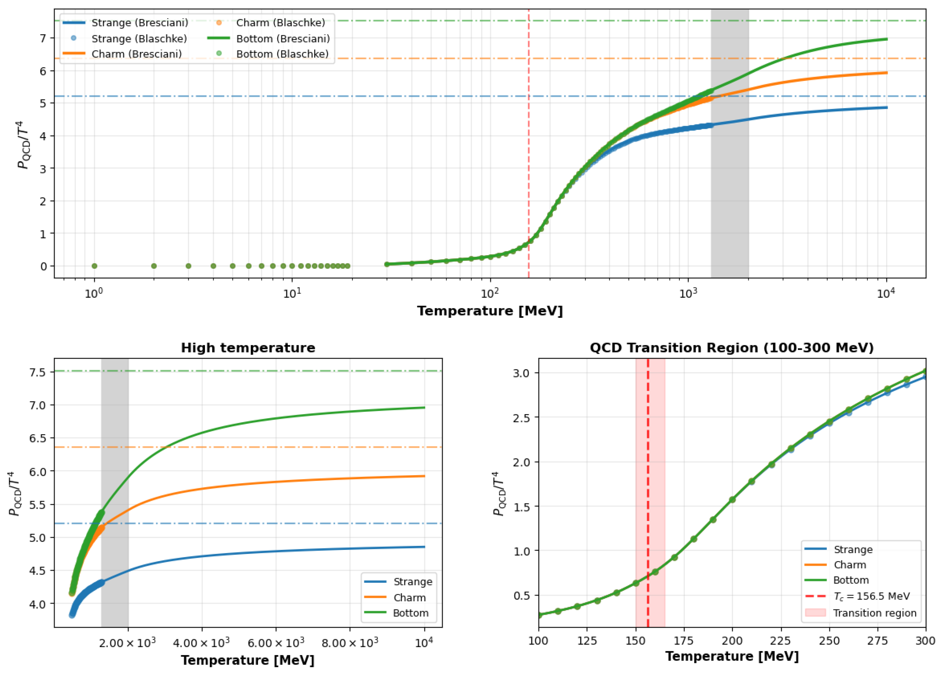
In Figure A1, we show different base pressures from the microscopical model and Bresciani in blue, and in orange and green, the tree-level evaluation using Equation (6). We can see how little impact the addition of heavy quarks has on the QCD transition at . The EW scale is not considered here, as it could be the baryogenesis and/or leptogenesis era, making the evolution of the thermodynamic quantities very model dependent [24]. The charge conservation Equations Equations (7)–(9) would not apply with the left-hand side as constant values. Bresciani et al. [72] and the microscopical data rely on different assumptions; a simple concatenation at exhibits a discontinuity. At , the microscopical model has not been compared with lattice QCD data; is therefore the highest reliable temperature of our microscopical model. We tried different interpolation ranges and found out that a concatenation at is the smallest temperature for which a smooth connection is possible for the three thermodynamic quantities s, and P. For consistency, we want to interpolate the three thermodynamic quantities on the exact same temperature range. The orange curve corresponds to the base data used to compute the cosmic trajectories (Section 3 and Section 4). The green curve is the one used in Figure 1 and Figure 8.
Figure A1.
Base QCD pressure for different numbers of quark flavors; the legend shows the heaviest quark of each configuration. Dots represent the base pressure from Ref. [43] down to MeV. The dash-dotted lines correspond to the SB limits, while the continuous lines show the data used for cosmic trajectory calculations; for , we used the polynomial extrapolation from Ref. [72], and the microscopical data extends up to . We rely on PCHIP interpolation, marked with the gray shaded region. In the bottom right plot, the three configurations overlaps.
Appendix B. More Cosmic Trajectories
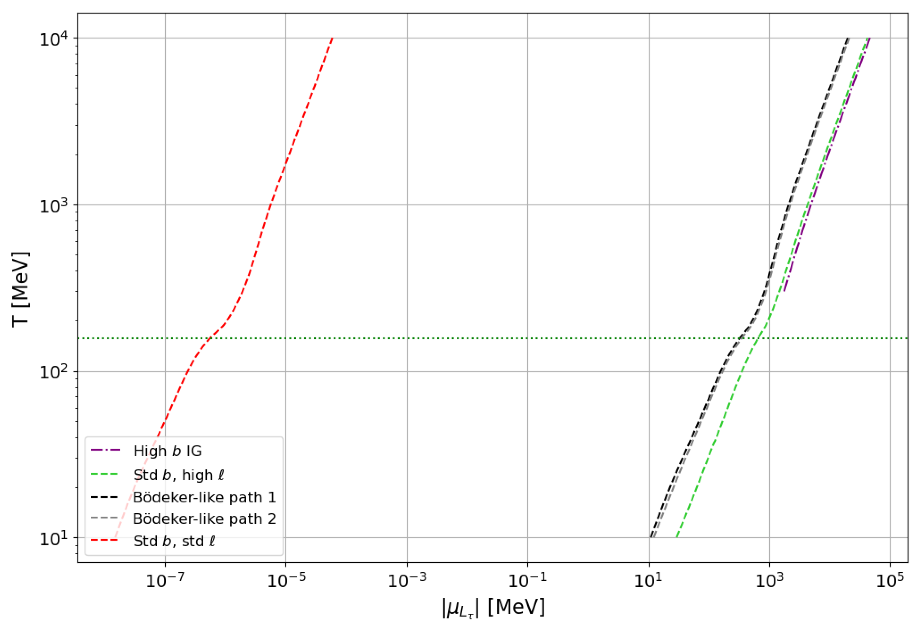
In Section 2, we presented the equations to solve and the induced cosmic trajectories in the T vs. plane. Since the system of equations is solved in the direction of the five chemical potentials, we show in this Appendix the cosmic trajectories in the other directions. Neutrinos and their associated charged leptons are linked according to Equation (12). Comparing the magnitude of Figure A3 and Figure A2, it becomes obvious that is small. The same analysis can be done for muon and tau leptons. In “Bödeker-like 2”, gains a significant value at large temperature, while for “Std b, high ℓ”, the bounce at the QCD transition lets gain value before vanishing at low temperature. For completeness, we show the cosmic trajectories in T vs. in Figure A4 and in T vs. Figure A5.
We also observe the difference in behavior between “Bödeker-like 1” and “Bödeker-like 2” in the T vs. plane, where the former don’t have asymmetry in the electronic sector, and the latter does, which shows a similar behavior to "Std b, high ℓ".
Figure A2.
Trajectories in the T vs. plane. The trajectories with fixed are not shown, as is ignored. If a trajectory were on the right on , it would indicate the formation of a pion condensate.
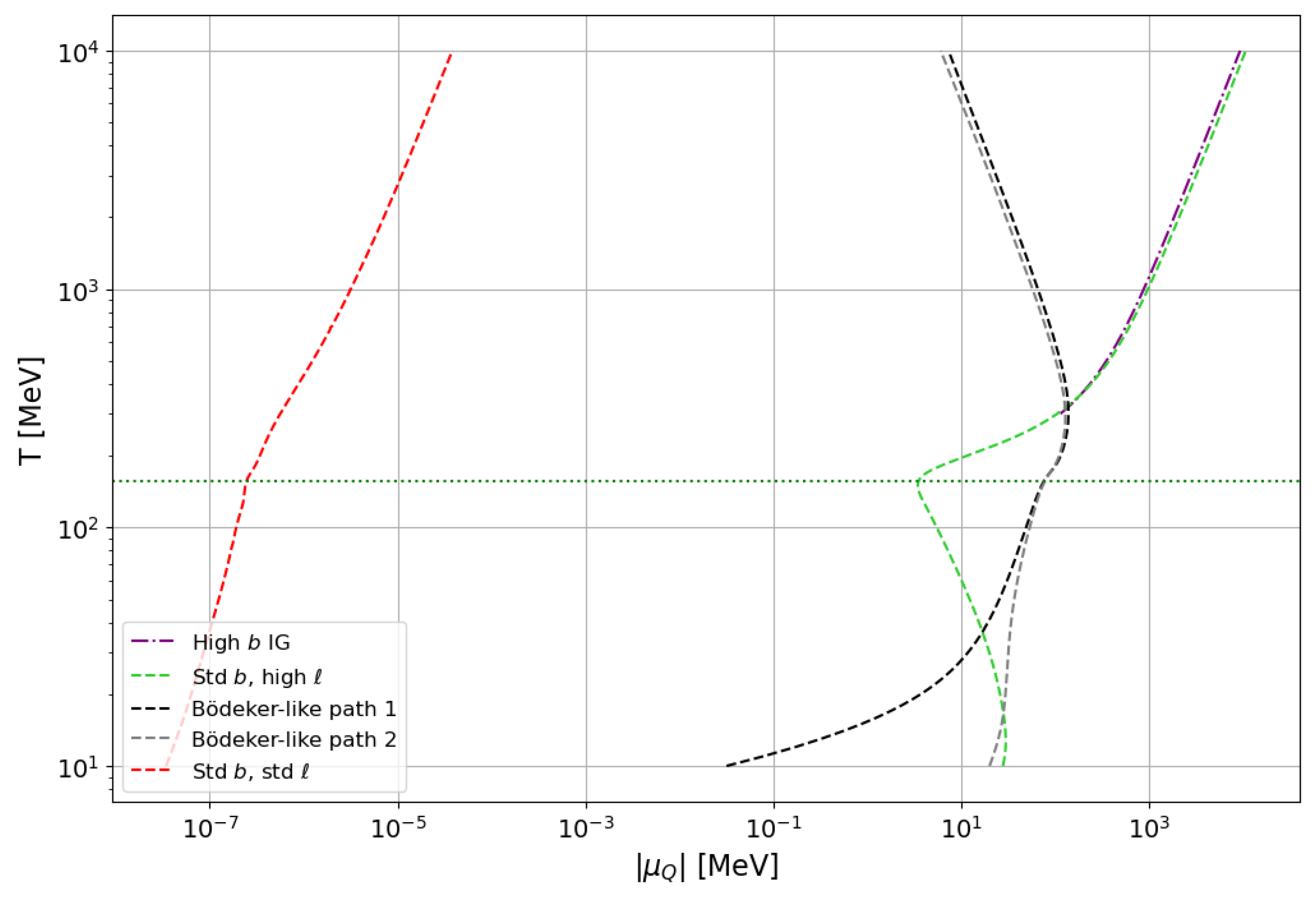
Figure A3.
Trajectories in the T vs. plane.
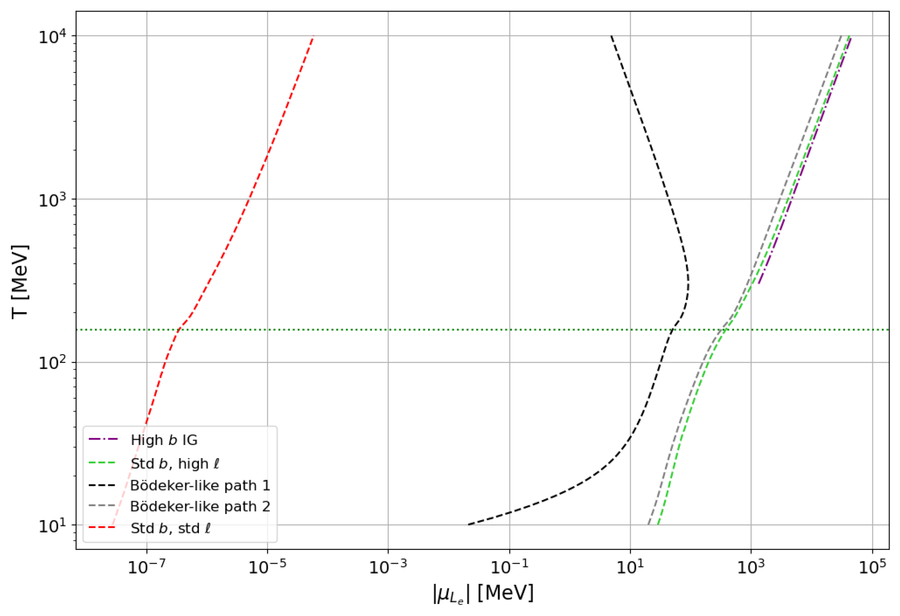
Figure A4.
Trajectories in the T vs. plane. “High b IG”, “Std b, high ℓ” and “Bödeker-like 2” exhibit positive chemical potential as the muon asymmetry is positive; for “Bödeker-like 1” and “Std b, std ℓ”, we show .
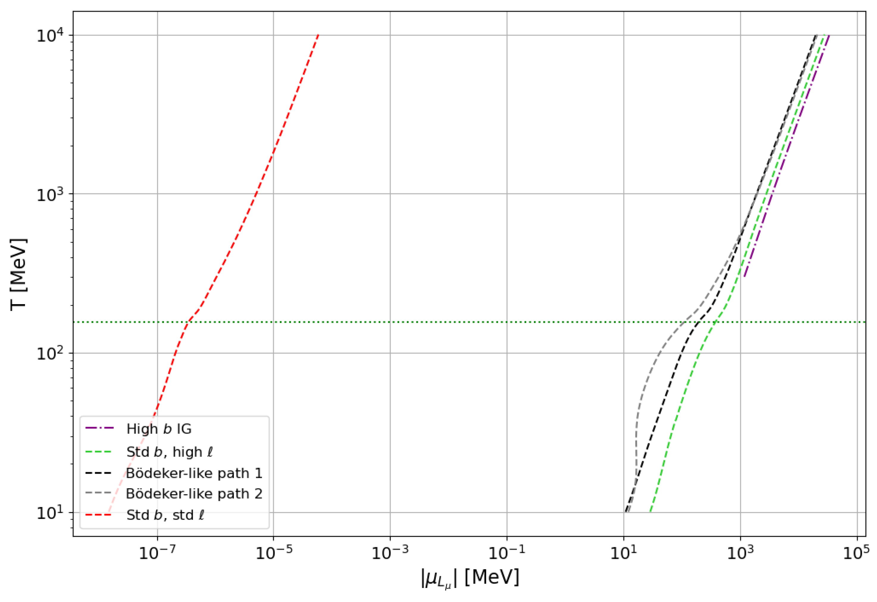
Figure A5.
Trajectories in the T vs. plane. “Bödeker-like 1” and “Bödeker-like 2” exhibit positive chemical potential as the tau asymmetry is positive; for the remaining model, we show .
References
- Abbott, R.; Abe, H.; Acernese, F.; Ackley, K.; Adhicary, S.; Adhikari, N.; Adhikari, R.X.; Adkins, V.K.; Adya, V.B.; Affeldt, C.; et al. Search for subsolar-mass black hole binaries in the second part of Advanced LIGO’s and Advanced Virgo’s third observing run. Mon. Not. R. Astron. Soc. 2023, 524, 5984–5992, Erratum in Mon. Not. R. Astron. Soc. 2023, 526, 6234. https://doi.org/10.1093/mnras/stad588.. [Google Scholar]
- The LIGO Scientific Collaboration; the Virgo Collaboration; the KAGRA Collaboration; Abac, A.G.; Abouelfettouh, I.; Acernese, F.; Ackley, K.; Adamcewicz, C.; Adhicary, S.; Adhikari, D.; et al. Search for planetary-mass ultra-compact binaries using data from the first part of the LIGO–Virgo–KAGRA fourth observing run. arXiv 2025, arXiv:2511.19911. [Google Scholar] [CrossRef] [Scilit]
- Kacanja, K.; Soni, K.; Akyüz, A.; Nitz, A.H. Search for Sub-Solar Mass Binaries in the First Part of LIGO’s Fourth Observing Run. arXiv 2026, arXiv:2602.12115. [Google Scholar] [CrossRef] [Scilit]
- Bagui, E.; Clesse, S.; De Luca, V.; Ezquiaga, J.M.; Franciolini, G.; García-Bellido, J.; Joana, C.; Kumar Jain, R.; Kuroyanagi, S.; Musco, I.; et al. Primordial black holes and their gravitational-wave signatures. Living Rev. Relativ. 2025, 28, 1. [Google Scholar] [CrossRef] [Scilit] [PubMed]
- Ligo Scientific Collaboration; VIRGO Collaboration; Kagra Collaboration. LIGO/Virgo/KAGRA S251112cm: Identification of a GW compact binary merger candidate. GRB Coord. Netw. 2025, 42650, 1. [Google Scholar]
- Carr, B.; Iovino, A.J.; Perna, G.; Vaskonen, V.; Veermäe, H. Primordial black holes: Constraints, potential evidence and prospects. arXiv 2026, arXiv:2601.06024. [Google Scholar] [CrossRef] [Scilit]
- Kasliwal, M.M.; Ahumada, T.; Stein, R.; Karambelkar, V.; Hall, X.J.; Singh, A.; Fremling, C.; Metzger, B.D.; Bulla, M.; Swain, V.; et al. ZTF25abjmnps (AT2025ulz) and S250818k: A Candidate Superkilonova from a Subthreshold Subsolar Gravitational-wave Trigger. Astrophys. J. Lett. 2025, 995, L59. [Google Scholar] [CrossRef] [Scilit]
- Carr, B.J.; Hawking, S.W. Black holes in the early Universe. Mon. Not. R. Astron. Soc. 1974, 168, 399–415. [Google Scholar] [CrossRef] [Scilit]
- Carr, B.J. The Primordial black hole mass spectrum. Astrophys. J. 1975, 201, 1–19. [Google Scholar] [CrossRef] [Scilit] [PubMed]
- Byrnes, C.T.; Hindmarsh, M.; Young, S.; Hawkins, M.R.S. Primordial black holes with an accurate QCD equation of state. J. Cosmol. Astropart. Phys. 2018, 08, 041. [Google Scholar] [CrossRef] [Scilit]
- Musco, I.; Jedamzik, K.; Young, S. Primordial black hole formation during the QCD phase transition: Threshold, mass distribution, and abundance. Phys. Rev. D 2024, 109, 083506. [Google Scholar] [CrossRef] [Scilit]
- Gonin, M.; Hasinger, G.; Blaschke, D.; Ivanytskyi, O.; Röpke, G. Primordial black-hole formation and heavy r-process element synthesis from the cosmological QCD transition. Eur. Phys. J. A 2025, 61, 170. [Google Scholar] [CrossRef] [Scilit]
- Carr, B.; Kuhnel, F. Primordial Black Holes as Dark Matter: Recent Developments. Ann. Rev. Nucl. Part. Sci. 2020, 70, 355–394. [Google Scholar] [CrossRef] [Scilit]
- Carr, B.; Kohri, K.; Sendouda, Y.; Yokoyama, J. Constraints on primordial black holes. Rept. Prog. Phys. 2021, 84, 116902. [Google Scholar] [CrossRef] [Scilit] [PubMed]
- Carr, B.; Clesse, S.; García-Bellido, J.; Kühnel, F. Cosmic conundra explained by thermal history and primordial black holes. Phys. Dark Univ. 2021, 31, 100755. [Google Scholar] [CrossRef] [Scilit]
- Hasinger, G. Illuminating the dark ages: Cosmic backgrounds from accretion onto primordial black hole dark matter. J. Cosmol. Astropart. Phys. 2020, 07, 022. [Google Scholar] [CrossRef] [Scilit]
- Borsanyi, S.; Fodor, Z.; Guenther, J.; Kampert, K.H.; Katz, S.D.; Kawanai, T.; Kovacs, T.G.; Mages, S.W.; Pasztor, A.; Pittler, F.; et al. Calculation of the axion mass based on high-temperature lattice quantum chromodynamics. Nature 2016, 539, 69–71. [Google Scholar] [CrossRef] [Scilit] [PubMed]
- Pandav, A. Experimental status of QCD phase diagram. J. Subat. Part. Cosmol. 2025, 4, 100167. [Google Scholar] [CrossRef] [Scilit]
- Hindmarsh, M.B.; Lüben, M.; Lumma, J.; Pauly, M. Phase transitions in the early universe. SciPost Phys. Lect. Notes 2021, 24, 1. [Google Scholar] [CrossRef] [Scilit]
- Guenther, J.N. Overview of the QCD phase diagram: Recent progress from the lattice. Eur. Phys. J. A 2021, 57, 136. [Google Scholar] [CrossRef] [Scilit] [PubMed]
- Guenther, J.N. An overview of the QCD phase diagram at finite T and μ. Proc. Sci. 2022, LATTICE2021, 013. [Google Scholar] [CrossRef] [Scilit]
- Lu, Y.; Gao, F.; Fu, B.; Song, H.; Liu, Y.X. Constructing the equation of state of QCD in a functional QCD based scheme. Phys. Rev. D 2024, 109, 114031. [Google Scholar] [CrossRef] [Scilit]
- Correia, J.; Hindmarsh, M.; Rummukainen, K.; Weir, D.J. Gravitational waves from strong first-order phase transitions. Phys. Rev. D 2025, 112, 123546. [Google Scholar] [CrossRef] [Scilit]
- Bodeker, D.; Buchmuller, W. Baryogenesis from the weak scale to the grand unification scale. Rev. Mod. Phys. 2021, 93, 035004. [Google Scholar] [CrossRef] [Scilit]
- van de Vis, J.; de Vries, J.; Postma, M. Bubble Trouble: A Review on Electroweak Baryogenesis. arXiv 2025, arXiv:2508.09989. [Google Scholar] [CrossRef] [Scilit]
- Sakharov, A.D. Violation of CP Invariance, C asymmetry, and baryon asymmetry of the universe. Pisma Zh. Eksp. Teor. Fiz. 1967, 5, 32–35. [Google Scholar] [CrossRef] [Scilit]
- Workman, R.L.; Burkert, V.D.; Crede, V.; Klempt, E.; Thoma, U.; Tiator, L.; Agashe, K.; Aielli, G.; Allanach, B.C.; Amsler, C.; et al. Review of Particle Physics. Prog. Theor. Exp. Phys. 2022, 2022, 083C01. [Google Scholar] [CrossRef] [Scilit]
- Kajantie, K.; Laine, M.; Rummukainen, K.; Shaposhnikov, M.E. Is there a hot electroweak phase transition at mH ≳ mW? Phys. Rev. Lett. 1996, 77, 2887–2890. [Google Scholar] [CrossRef] [Scilit] [PubMed]
- Kajantie, K.; Laine, M.; Rummukainen, K.; Shaposhnikov, M.E. A Nonperturbative analysis of the finite T phase transition in SU(2) x U(1) electroweak theory. Nucl. Phys. B 1997, 493, 413–438. [Google Scholar] [CrossRef] [Scilit]
- Boeckel, T.; Schettler, S.; Schaffner-Bielich, J. The Cosmological QCD Phase Transition Revisited. Prog. Part. Nucl. Phys. 2011, 66, 266–270. [Google Scholar] [CrossRef] [Scilit]
- Boeckel, T.; Schaffner-Bielich, J. A little inflation at the cosmological QCD phase transition. Phys. Rev. D 2012, 85, 103506. [Google Scholar] [CrossRef] [Scilit]
- Iso, S.; Serpico, P.D.; Shimada, K. QCD-Electroweak First-Order Phase Transition in a Supercooled Universe. Phys. Rev. Lett. 2017, 119, 141301. [Google Scholar] [CrossRef] [Scilit] [PubMed]
- Khlopov, M. What comes after the Standard Model? Prog. Part. Nucl. Phys. 2021, 116, 103824. [Google Scholar] [CrossRef] [Scilit]
- Schwarz, D.J.; Stuke, M. Lepton asymmetry and the cosmic QCD transition. J. Cosmol. Astropart. Phys. 2009, 11, 025, Erratum in J. Cosmol. Astropart. Phys. 2010, 10, E01. https://doi.org/10.1088/1475-7516/2009/11/025.. [Google Scholar] [CrossRef] [Scilit]
- March-Russell, J.; Murayama, H.; Riotto, A. The Small observed baryon asymmetry from a large lepton asymmetry. J. High Energy Phys. 1999, 11, 015. [Google Scholar] [CrossRef] [Scilit]
- Barenboim, G.; Park, W.I. A full picture of large lepton number asymmetries of the Universe. J. Cosmol. Astropart. Phys. 2017, 04, 048. [Google Scholar] [CrossRef] [Scilit]
- Gao, F.; Oldengott, I.M. Cosmology Meets Functional QCD: First-Order Cosmic QCD Transition Induced by Large Lepton Asymmetries. Phys. Rev. Lett. 2022, 128, 131301. [Google Scholar] [CrossRef] [Scilit] [PubMed]
- Gao, F.; Harz, J.; Hati, C.; Lu, Y.; Oldengott, I.M.; White, G. Sphaleron freeze-in baryogenesis with gravitational waves from the QCD transition. Phys. Lett. B 2025, 869, 139849. [Google Scholar] [CrossRef] [Scilit]
- Gao, F.; Harz, J.; Hati, C.; Lu, Y.; Oldengott, I.M.; White, G. Baryogenesis and first-order QCD transition with gravitational waves from a large lepton asymmetry. J. High Energy Phys. 2025, 06, 247. [Google Scholar] [CrossRef] [Scilit]
- Barenboim, G.; Kinney, W.H.; Park, W.I. Resurrection of large lepton number asymmetries from neutrino flavor oscillations. Phys. Rev. D 2017, 95, 043506. [Google Scholar] [CrossRef] [Scilit]
- Froustey, J.; Pitrou, C. Constraints on primordial lepton asymmetries with full neutrino transport. Phys. Rev. D 2024, 110, 103551. [Google Scholar] [CrossRef] [Scilit]
- Bödeker, D.; Kühnel, F.; Oldengott, I.M.; Schwarz, D.J. Lepton flavor asymmetries and the mass spectrum of primordial black holes. Phys. Rev. D 2021, 103, 063506. [Google Scholar] [CrossRef] [Scilit]
- Blaschke, D.; Cierniak, M.; Ivanytskyi, O.; Röpke, G. Thermodynamics of quark matter with multiquark clusters in an effective Beth-Uhlenbeck type approach. Eur. Phys. J. A 2024, 60, 14. [Google Scholar] [CrossRef] [Scilit]
- Formaggio, L.; Di Clemente, F.; Yadav, G.; Drago, A.; Ratti, C. Cosmic trajectories calculation with a state of the art lattice QCD equation of state. Phys. Rev. D 2026, 113, 023522. [Google Scholar] [CrossRef] [Scilit]
- Rafelski, J.; Birrell, J.; Grayson, C.; Steinmetz, A.; Yang, C.T. Quarks to Cosmos: Particles and plasma in cosmological evolution. Eur. Phys. J. Spec. Top. 2025, 234, 1125–1329. [Google Scholar] [CrossRef] [Scilit]
- Husdal, L. On Effective Degrees of Freedom in the Early Universe. Galaxies 2016, 4, 78. [Google Scholar] [CrossRef] [Scilit]
- Guth, A.H. The Inflationary Universe: A Possible Solution to the Horizon and Flatness Problems. Phys. Rev. D 1981, 23, 347–356. [Google Scholar] [CrossRef] [Scilit]
- Bazavov, A.; Ding, H.T.; Hegde, P.; Kaczmarek, O.; Karsch, F.; Karthik, N.; Laermann, E.; Lahiri, A.; Larsen, R.; Li, S.T.; et al. Chiral crossover in QCD at zero and non-zero chemical potentials. Phys. Lett. B 2019, 795, 15–21. [Google Scholar] [CrossRef] [Scilit]
- Sharma, S.; Karsch, F.; Petreczky, P. Thermodynamics of charmed hadrons across chiral crossover from lattice QCD. J. Subat. Part. Cosmol. 2025, 3, 100044. [Google Scholar] [CrossRef] [Scilit]
- Kaczmarek, O.; Karsch, F.; Petreczky, P.; Schmidt, C.; Sharma, S. Generalized susceptibilities and the properties of charm degrees of freedom across the QCD crossover temperature. Phys. Rev. D 2025, 112, 034509. [Google Scholar] [CrossRef] [Scilit]
- Laine, M.; Meyer, M. Standard Model thermodynamics across the electroweak crossover. J. Cosmol. Astropart. Phys. 2015, 07, 035. [Google Scholar] [CrossRef] [Scilit]
- Escudero Abenza, M. Precision early universe thermodynamics made simple: Neff and neutrino decoupling in the Standard Model and beyond. J. Cosmol. Astropart. Phys. 2020, 05, 048. [Google Scholar] [CrossRef] [Scilit]
- Escudero, M.; Jackson, G.; Laine, M.; Sandner, S. Fast and flexible neutrino decoupling. Part I. The Standard Model. J. Cosmol. Astropart. Phys. 2026, 02, 046. [Google Scholar] [CrossRef] [Scilit]
- Crivellin, A.; Mellado, B. Anomalies in Particle Physcis. PoS 2025, DIS2024, 007. [Google Scholar] [CrossRef] [Scilit]
- Krasznahorkay, A.J.; Krasznahorkay, A.; Csatlós, M.; Timár, J.; Begala, M.; Krakó, A.; Rajta, I.; Vajda, I.; Sas, N.J. An Update of the Hypothetical X17 Particle. Universe 2024, 10, 409. [Google Scholar] [CrossRef] [Scilit]
- Alves, D.S.M.; Barducci, D.; Cavoto, G.; Darmé, L.; Delle Rose, L.; Doria, L.; Feng, J.L.; Frankenthal, A.; Gasparian, A.; Goudzovski, E.; et al. Shedding light on X17: Community report. Eur. Phys. J. C 2023, 83, 230. [Google Scholar] [CrossRef] [Scilit]
- Aghanim, N.; Akrami, Y.; Ashdown, M.; Aumont, J.; Baccigalupi, C.; Ballardini, M.; Banday, A.J.; Barreiro, R.B.; Bartolo, N.; Basak, S.; et al. Planck 2018 results. VI. Cosmological parameters. Astron. Astrophys. 2020, 641, A6, Erratum in Astron. Astrophys. 2021, 652, C4. https://doi.org/10.1051/0004-6361/201833910.. [Google Scholar] [CrossRef] [Scilit]
- Harvey, J.A.; Turner, M.S. Cosmological Baryon and Lepton Number in the Presence of Electroweak Fermion Number Violation. Phys. Rev. D 1990, 42, 3344–3349. [Google Scholar] [CrossRef] [Scilit] [PubMed]
- Allahverdi, R.; Mazumdar, A. A mini review on Affleck-Dine baryogenesis. New J. Phys. 2012, 14, 125013. [Google Scholar] [CrossRef] [Scilit]
- Kasai, K.; Kawasaki, M.; Murai, K. Revisiting the Affleck-Dine mechanism for primordial black hole formation. J. Cosmol. Astropart. Phys. 2022, 10, 048. [Google Scholar] [CrossRef] [Scilit]
- Oldengott, I.M.; Schwarz, D.J. Improved constraints on lepton asymmetry from the cosmic microwave background. EPL 2017, 119, 29001. [Google Scholar] [CrossRef] [Scilit]
- Kawasaki, M.; Murai, K. Lepton asymmetric universe. J. Cosmol. Astropart. Phys. 2022, 08, 041. [Google Scholar] [CrossRef] [Scilit]
- Escudero, M.; Ibarra, A.; Maura, V. Primordial lepton asymmetries in the precision cosmology era: Current status and future sensitivities from BBN and the CMB. Phys. Rev. D 2023, 107, 035024. [Google Scholar] [CrossRef] [Scilit]
- Lattanzi, M.; Moretti, M. Lepton Asymmetries in Cosmology. Symmetry 2024, 16, 1657. [Google Scholar] [CrossRef] [Scilit]
- Li, Y.Z.; Yu, J.H. Primordial lepton asymmetries: Neutrino transport, spectral distortions and cosmological constraints. J. High Energy Phys. 2025, 06, 213. [Google Scholar] [CrossRef] [Scilit]
- Akita, K.; Hamaguchi, K.; Ovchynnikov, M. Affleck-Dine leptoflavorgenesis. J. High Energy Phys. 2025, 12, 142. [Google Scholar] [CrossRef] [Scilit]
- Domcke, V.; Escudero, M.; Fernandez Navarro, M.; Sandner, S. Lepton flavor asymmetries: From the early Universe to BBN. J. High Energy Phys. 2025, 06, 137. [Google Scholar] [CrossRef] [Scilit]
- Wygas, M.M.; Oldengott, I.M.; Bödeker, D.; Schwarz, D.J. Cosmic QCD Epoch at Nonvanishing Lepton Asymmetry. Phys. Rev. Lett. 2018, 121, 201302. [Google Scholar] [CrossRef] [Scilit] [PubMed]
- Wygas, M.M. Large Lepton Asymmetry and the Cosmic QCD Transition. Ph.D. Thesis, Bielefeld University (Germany), Bielefeld, Germany, 2019. [Google Scholar]
- Abuali, A.; Borsányi, S.; Fodor, Z.; Jahan, J.; Kahangirwe, M.; Parotto, P.; Pásztor, A.; Ratti, C.; Shah, H.; Trabulsi, S.A. New 4D lattice QCD equation of state: Extended density coverage from a generalized T’ expansion. Phys. Rev. D 2025, 112, 054502. [Google Scholar] [CrossRef] [Scilit]
- Johns, S.M.; Ellis, P.J.; Lattimer, J.M. Numerical approximation to the thermodynamic integrals. Astrophys. J. 1996, 473, 1020–1028. [Google Scholar] [CrossRef] [Scilit]
- Bresciani, M.; Brida, M.D.; Giusti, L.; Pepe, M. QCD Equation of State with Nf=3 Flavors up to the Electroweak Scale. Phys. Rev. Lett. 2025, 134, 201904. [Google Scholar] [CrossRef] [Scilit] [PubMed]
- Vovchenko, V.; Stoecker, H. Thermal-FIST: A package for heavy-ion collisions and hadronic equation of state. Comput. Phys. Commun. 2019, 244, 295–310. [Google Scholar] [CrossRef] [Scilit]
- Bazavov, A.; Petreczky, P.; Weber, J.H. Equation of State in 2+1 Flavor QCD at High Temperatures. Phys. Rev. D 2018, 97, 014510. [Google Scholar] [CrossRef] [Scilit]
- Caprini, C.; Biller, S.; Ferreira, P.G. Constraints on the electrical charge asymmetry of the universe. J. Cosmol. Astropart. Phys. 2005, 02, 006. [Google Scholar] [CrossRef] [Scilit]
- Blaschke, D.; Liebing, S.; Röpke, G.; Dönigus, B. Cluster production and the chemical freeze-out in expanding hot dense matter. Phys. Lett. B 2025, 860, 139206. [Google Scholar] [CrossRef] [Scilit]
- Middeldorf-Wygas, M.M.; Oldengott, I.M.; Bödeker, D.; Schwarz, D.J. Cosmic QCD transition for large lepton flavor asymmetries. Phys. Rev. D 2022, 105, 123533. [Google Scholar] [CrossRef] [Scilit]
- Vovchenko, V.; Brandt, B.B.; Cuteri, F.; Endrődi, G.; Hajkarim, F.; Schaffner-Bielich, J. Pion Condensation in the Early Universe at Nonvanishing Lepton Flavor Asymmetry and Its Gravitational Wave Signatures. Phys. Rev. Lett. 2021, 126, 012701. [Google Scholar] [CrossRef] [Scilit] [PubMed]
- Ferreira, O.; Fraga, E.S.; Hippert, M.; Schaffner-Bielich, J. Chiral symmetry breaking and pion condensation in the early Universe. Phys. Rev. D 2025, 112, 094009. [Google Scholar] [CrossRef] [Scilit]
- Di Clemente, F.; Drago, A.; Formaggio, L.; Ratti, C.; Vovchenko, V.; Yadav, G. Upper Bound on the Cosmic Baryon Chemical Potential from Lepton-Flavor Asymmetry. arXiv 2025, arXiv:2511.11995. [Google Scholar] [CrossRef] [Scilit]
- Escrivà, A.; Bagui, E.; Clesse, S. Simulations of PBH formation at the QCD epoch and comparison with the GWTC-3 catalog. J. Cosmol. Astropart. Phys. 2023, 05, 004. [Google Scholar] [CrossRef] [Scilit]
- Escrivà, A. Simulation of primordial black hole formation using pseudo-spectral methods. Phys. Dark Univ. 2020, 27, 100466. [Google Scholar] [CrossRef] [Scilit]
- Musco, I.; Miller, J.C.; Rezzolla, L. Computations of primordial black hole formation. Class. Quant. Grav. 2005, 22, 1405–1424. [Google Scholar] [CrossRef] [Scilit]
- Musco, I.; Miller, J.C. Primordial black hole formation in the early universe: Critical behaviour and self-similarity. Class. Quant. Grav. 2013, 30, 145009. [Google Scholar] [CrossRef] [Scilit]
- Escrivà, A. PBH Formation from Spherically Symmetric Hydrodynamical Perturbations: A Review. Universe 2022, 8, 66. [Google Scholar] [CrossRef] [Scilit]
- Braglia, M.; Garcia-Bellido, J.; Kuroyanagi, S. Testing Primordial Black Holes with multi-band observations of the stochastic gravitational wave background. J. Cosmol. Astropart. Phys. 2021, 12, 012. [Google Scholar] [CrossRef] [Scilit]
- Choptuik, M.W. Universality and scaling in gravitational collapse of a massless scalar field. Phys. Rev. Lett. 1993, 70, 9–12. [Google Scholar] [CrossRef] [Scilit] [PubMed]
- Niemeyer, J.C.; Jedamzik, K. Dynamics of primordial black hole formation. Phys. Rev. D 1999, 59, 124013. [Google Scholar] [CrossRef] [Scilit]
- Germani, C.; Sheth, R.K. The Statistics of Primordial Black Holes in a Radiation-Dominated Universe: Recent and New Results. Universe 2023, 9, 421. [Google Scholar] [CrossRef] [Scilit]
- Yoo, C.M.; Harada, T.; Hirano, S.; Kohri, K. Abundance of Primordial Black Holes in Peak Theory for an Arbitrary Power Spectrum. Prog. Theor. Exp. Phys. 2021, 2021, 013E02, Erratum in Prog. Theor. Exp. Phys. 2024, 2024, 049203. https://doi.org/10.1093/ptep/ptaa155.. [Google Scholar] [CrossRef] [Scilit]
- Escriva, A.; Tada, Y.; Yoo, C.M. Primordial black holes and induced gravitational waves from a smooth crossover beyond standard model theories. Phys. Rev. D 2024, 110, 063521. [Google Scholar] [CrossRef] [Scilit]
- The LIGO Scientific Collaboration; the Virgo Collaboration; the KAGRA Collaboration; Abac, A.G.; Abouelfettouh, I.; Acernese, F.; Ackley, K.; Adamcewicz, C.; Adhicary, S.; Adhikari, D.; et al. GWTC-4.0: Updating the Gravitational-Wave Transient Catalog with Observations from the First Part of the Fourth LIGO-Virgo-KAGRA Observing Run. arXiv 2025, arXiv:2508.18082. [Google Scholar] [CrossRef] [Scilit]
- Ruiz-Rocha, K.; Yelikar, A.B.; Lange, J.; Gabella, W.; Weller, R.A.; O’Shaughnessy, R.; Holley-Bockelmann, K.; Jani, K. Properties of “Lite” Intermediate-mass Black Hole Candidates in LIGO-Virgo’s Third Observing Run. Astrophys. J. Lett. 2025, 985, L37. [Google Scholar] [CrossRef] [Scilit]
- Khlopov, M.Y.; Konoplich, R.V.; Rubin, S.G.; Sakharov, A.S. First-order phase transitions as a source of black holes in the early universe. Grav. Cosmol. 2000, 6, 153–156. [Google Scholar]
- Baker, M.J.; Breitbach, M.; Kopp, J.; Mittnacht, L. Primordial black holes from first-order cosmological phase transitions. Phys. Lett. B 2025, 868, 139625. [Google Scholar] [CrossRef] [Scilit]
- Vilenkin, A.; Levin, Y.; Gruzinov, A. Cosmic strings and primordial black holes. J. Cosmol. Astropart. Phys. 2018, 11, 008. [Google Scholar] [CrossRef] [Scilit]
- Hashino, K.; Kanemura, S.; Takahashi, T.; Tanaka, M. Probing first-order electroweak phase transition via primordial black holes in the effective field theory. Phys. Lett. B 2023, 838, 137688. [Google Scholar] [CrossRef] [Scilit]
- Green, A.M. Stellar microlensing as a probe of Primordial Black Holes: Status and prospects. arXiv 2026, arXiv:2602.15974. [Google Scholar] [CrossRef] [Scilit]
- Hawkins, M.R.S. A new look at microlensing limits on dark matter in the Galactic halo. Astron. Astrophys. 2015, 575, A107. [Google Scholar] [CrossRef] [Scilit]
- Alcock, C.; Allsman, R.A.; Alves, D.; Axelrod, T.S.; Becker, A.C.; Bennett, D.P.; Cook, K.H.; Freeman, K.C.; Griest, K.; Guern, J.; et al. The MACHO project LMC microlensing results from the first two years and the nature of the galactic dark halo. Astrophys. J. 1997, 486, 697–726. [Google Scholar] [CrossRef] [Scilit]
- Alcock, C.; Allsman, R.A.; Alves, D.R.; Axelrod, T.S.; Becker, A.C.; Bennett, D.P.; Cook, K.H.; Dalal, N.; Drake, A.J.; Freeman, K.C.; et al. The MACHO project: Microlensing results from 5.7 years of LMC observations. Astrophys. J. 2000, 542, 281–307. [Google Scholar] [CrossRef] [Scilit]
- Tisserand, P.; Le Guillou, L.; Afonso, C.; Albert, J.N.; Andersen, J.; Ansari, R.; Aubourg, É.; Bareyre, P.; Beaulieu, J.P.; Charlot, X.; et al. Limits on the Macho Content of the Galactic Halo from the EROS-2 Survey of the Magellanic Clouds. Astron. Astrophys. 2007, 469, 387–404. [Google Scholar] [CrossRef] [Scilit]
- Mróz, P.; Udalski, A.; Szymański, M.K.; Kapusta, M.; Soszyński, I.; Wyrzykowski, Ł.; Pietrukowicz, P.; Kozłowski, S.; Poleski, R.; Skowron, J.; et al. Microlensing Optical Depth and Event Rate toward the Large Magellanic Cloud Based on 20 yr of OGLE Observations. Astrophys. J. Suppl. Ser. 2024, 273, 4. [Google Scholar] [CrossRef] [Scilit]
- Mróz, P.; Udalski, A.; Szymański, M.K.; Soszyński, I.; Pietrukowicz, P.; Kozłowski, S.; Poleski, R.; Skowron, J.; Skowron, D.; Ulaczyk, K.; et al. Microlensing Optical Depth, Event Rate, and Limits on Compact Objects in Dark Matter Based on 20 Yr of OGLE Observations of the Small Magellanic Cloud. Astrophys. J. Suppl. Ser. 2025, 280, 49. [Google Scholar] [CrossRef] [Scilit]
- Garcia-Bellido, J.; Hawkins, M. Reanalysis of the MACHO Constraints on PBH in the Light of Gaia DR3 Data. Universe 2024, 10, 449. [Google Scholar] [CrossRef] [Scilit]
- Hawkins, M.R.S.; García-Bellido, J. A critical analysis of the recent OGLE limits on stellar mass primordial black holes in the halo of the Milky Way. Mon. Not. R. Astron. Soc. 2025, 544, 1950–1957. [Google Scholar] [CrossRef] [Scilit]
- Niikura, H.; Takada, M.; Yasuda, N.; Lupton, R.H.; Sumi, T.; More, S.; Kurita, T.; Sugiyama, S.; More, A.; Oguri, M.; et al. Microlensing constraints on primordial black holes with Subaru/HSC Andromeda observations. Nat. Astron. 2019, 3, 524–534. [Google Scholar] [CrossRef] [Scilit]
- Sugiyama, S.; Takada, M.; Yasuda, N.; Tominaga, N. Microlensing constraints on Primordial Black Hole abundance with Subaru Hyper Suprime-Cam observations of Andromeda. arXiv 2026, arXiv:2602.05840. [Google Scholar] [CrossRef] [Scilit]
- Esser, N.; Tinyakov, P. Constraints on primordial black holes from observation of stars in dwarf galaxies. Phys. Rev. D 2023, 107, 103052. [Google Scholar] [CrossRef]
- Esser, N.; García-Bellido, J.; Tinyakov, P. Gravitational waves from primordial black holes passing by neutron stars: Observational prospects for the Galactic center. arXiv 2026, arXiv:2602.23429. [Google Scholar] [CrossRef] [Scilit]
- Braglia, M.; Garcia-Bellido, J.; Kuroyanagi, S. Tracking the origin of black holes with the stochastic gravitational wave background popcorn signal. Mon. Not. R. Astron. Soc. 2023, 519, 6008–6019. [Google Scholar] [CrossRef] [Scilit]
- Franciolini, G.; Musco, I.; Pani, P.; Urbano, A. From inflation to black hole mergers and back again: Gravitational-wave data-driven constraints on inflationary scenarios with a first-principle model of primordial black holes across the QCD epoch. Phys. Rev. D 2022, 106, 123526. [Google Scholar] [CrossRef] [Scilit]
- Cecchini, C.; Franciolini, G.; Pieroni, M. Forecasting constraints on scalar-induced gravitational waves with future pulsar timing array observations. Phys. Rev. D 2025, 111, 123536. [Google Scholar] [CrossRef] [Scilit]
- Domènech, G. Scalar Induced Gravitational Waves Review. Universe 2021, 7, 398. [Google Scholar] [CrossRef] [Scilit]
- Clesse, S.; García-Bellido, J. Detecting the gravitational wave background from primordial black hole dark matter. Phys. Dark Univ. 2017, 18, 105–114. [Google Scholar] [CrossRef] [Scilit]
- Cyr, B.; Kite, T.; Chluba, J.; Hill, J.C.; Jeong, D.; Acharya, S.K.; Bolliet, B.; Patil, S.P. Disentangling the primordial nature of stochastic gravitational wave backgrounds with CMB spectral distortions. Mon. Not. R. Astron. Soc. 2024, 528, 883–897. [Google Scholar] [CrossRef] [Scilit]
- Agius, D.; Essig, R.; Gaggero, D.; Scarcella, F.; Suczewski, G.; Valli, M. Feedback in the dark: A critical examination of CMB bounds on primordial black holes. J. Cosmol. Astropart. Phys. 2024, 07, 003. [Google Scholar] [CrossRef] [Scilit]
- Nakama, T.; Carr, B.; Silk, J. Limits on primordial black holes from μ distortions in cosmic microwave background. Phys. Rev. D 2018, 97, 043525. [Google Scholar] [CrossRef] [Scilit]
- Pacucci, F.; Nguyen, B.; Carniani, S.; Maiolino, R.; Fan, X. JWST CEERS and JADES Active Galaxies at z = 4–7 Violate the Local M⊙–M⊙ Relation at >3σ: Implications for Low-mass Black Holes and Seeding Models. Astrophys. J. Lett. 2023, 957, L3. [Google Scholar] [CrossRef] [Scilit]
- Goulding, A.D.; Greene, J.E.; Setton, D.J.; Labbe, I.; Bezanson, R.; Miller, T.B.; Atek, H.; Bogdán, Á.; Brammer, G.; Chemerynska, I.; et al. UNCOVER: The Growth of the First Massive Black Holes from JWST/NIRSpec—Spectroscopic Redshift Confirmation of an X-Ray Luminous AGN at z = 10.1. Astrophys. J. Lett. 2023, 955, L24. [Google Scholar] [CrossRef] [Scilit]
- Larson, R.L.; Finkelstein, S.L.; Kocevski, D.D.; Hutchison, T.A.; Trump, J.R.; Arrabal Haro, P.; Bromm, V.; Cleri, N.J.; Dickinson, M.; Fujimoto, S.; et al. A CEERS Discovery of an Accreting Supermassive Black Hole 570 Myr after the Big Bang: Identifying a Progenitor of Massive z > 6 Quasars. Astrophys. J. Lett. 2023, 953, L29. [Google Scholar] [CrossRef] [Scilit]
- De Luca, V.; Del Grosso, L.; Franciolini, G.; Kritos, K.; Berti, E.; D’Orazio, D.; Silk, J. Primordial-Black-Hole-Based Pathways to Little Red Dots. Phys. Rev. Lett. 2026, 136, 231402. [Google Scholar] [CrossRef] [Scilit] [PubMed]
- Mack, K.J.; Ostriker, J.P.; Ricotti, M. Growth of structure seeded by primordial black holes. Astrophys. J. 2007, 665, 1277–1287. [Google Scholar] [CrossRef] [Scilit]
- Essick, R.; Coughlin, M.W.; Zevin, M.; Chatterjee, D.; Clarke, T.A.; Colloms, S.; Mali, U.; Miller, S.; Steinle, N.; Baral, P.; et al. Compact binary coalescence sensitivity estimates with injection campaigns during the LIGO-Virgo-KAGRA Collaborations’ fourth observing run. Phys. Rev. D 2025, 112, 102001. [Google Scholar] [CrossRef] [Scilit]
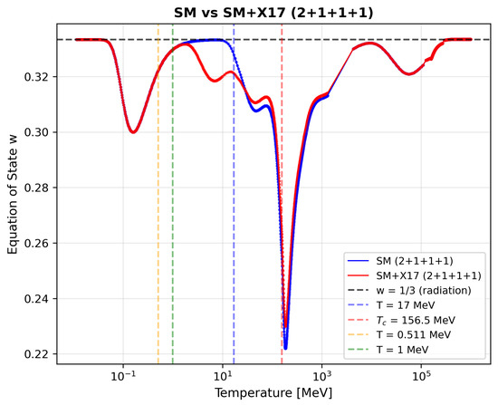
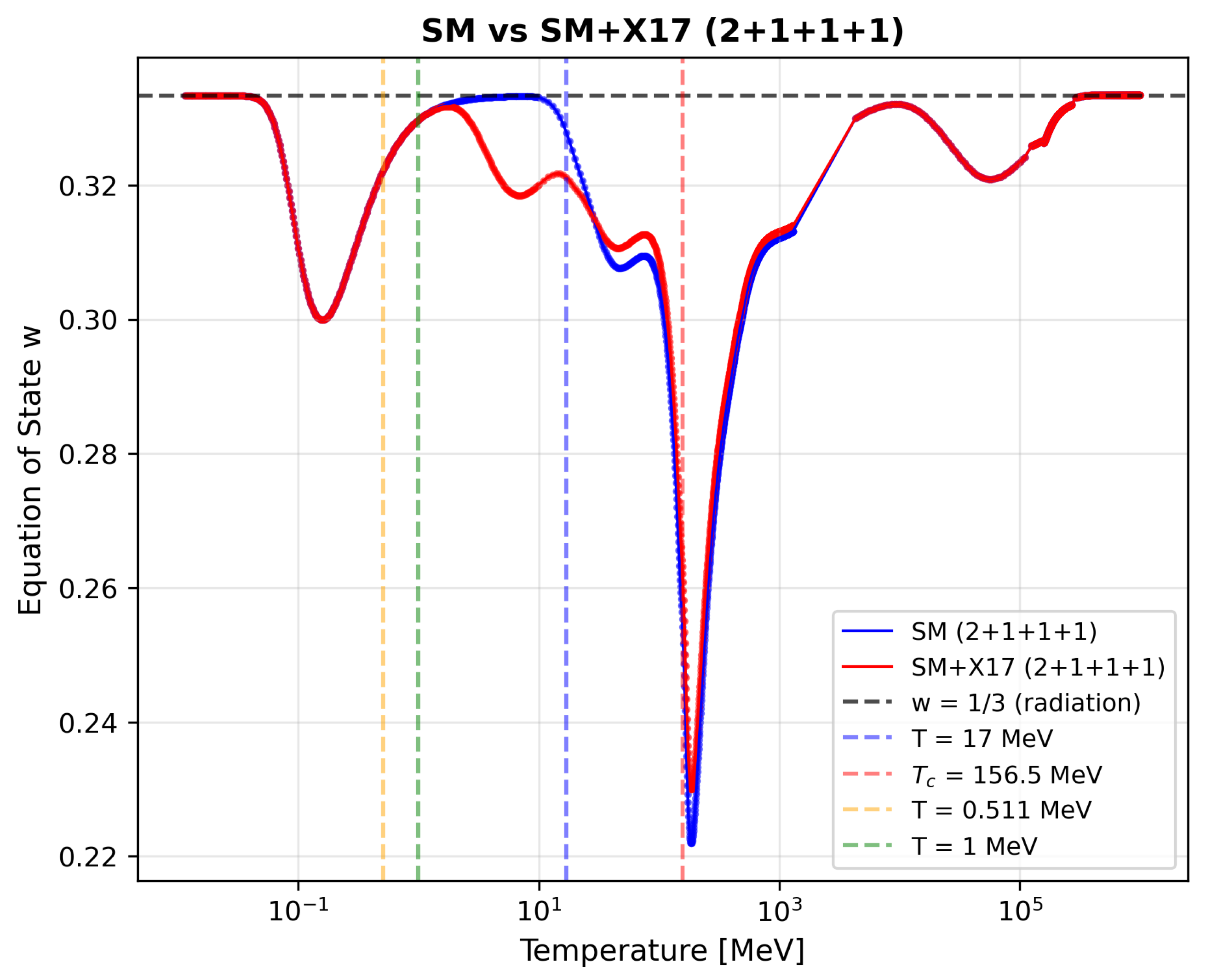
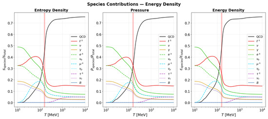
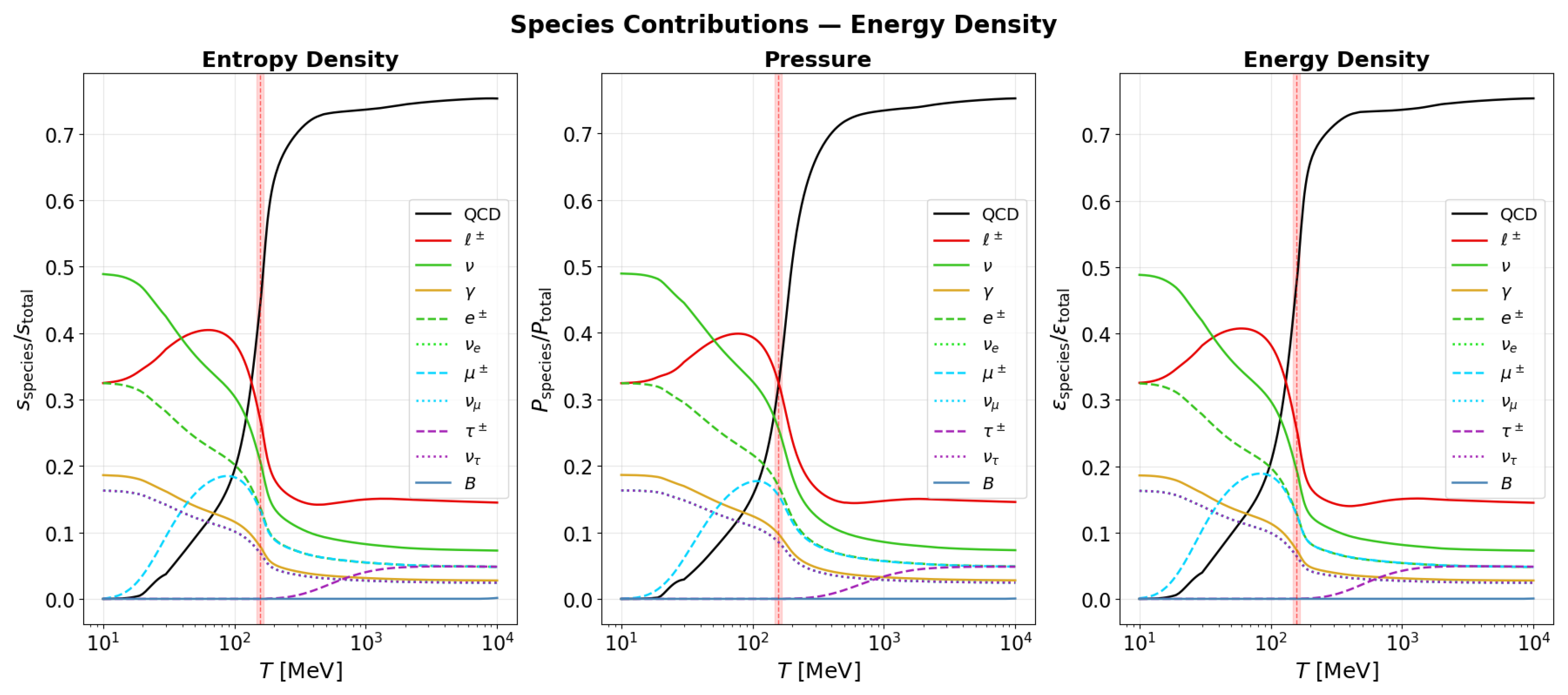
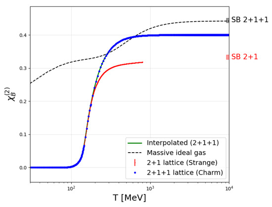
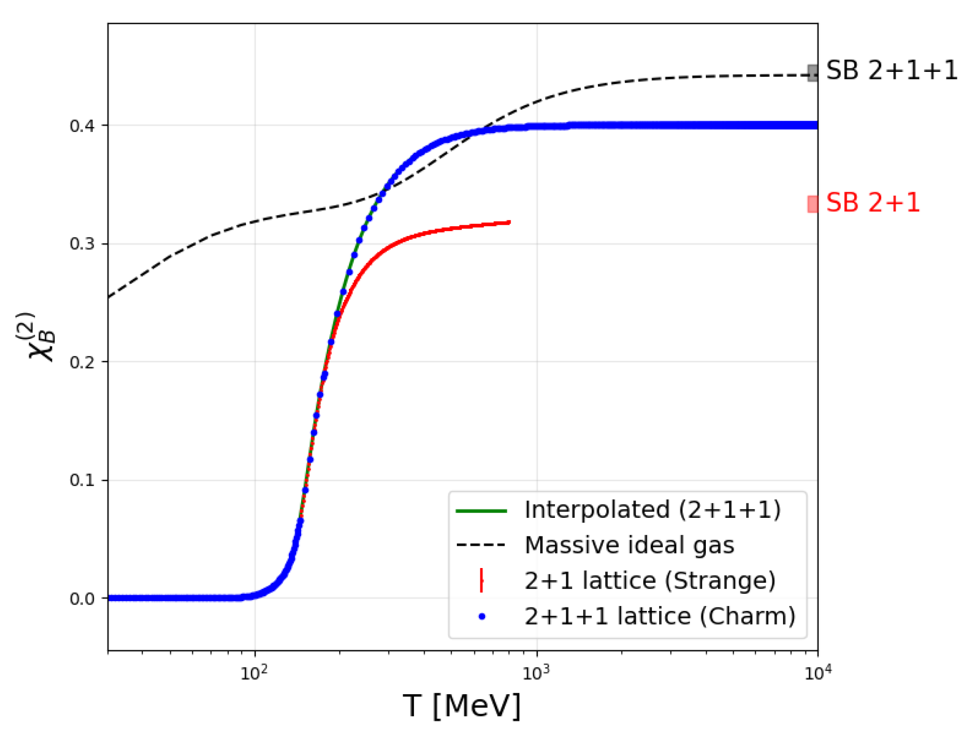
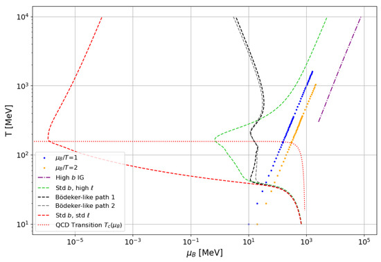
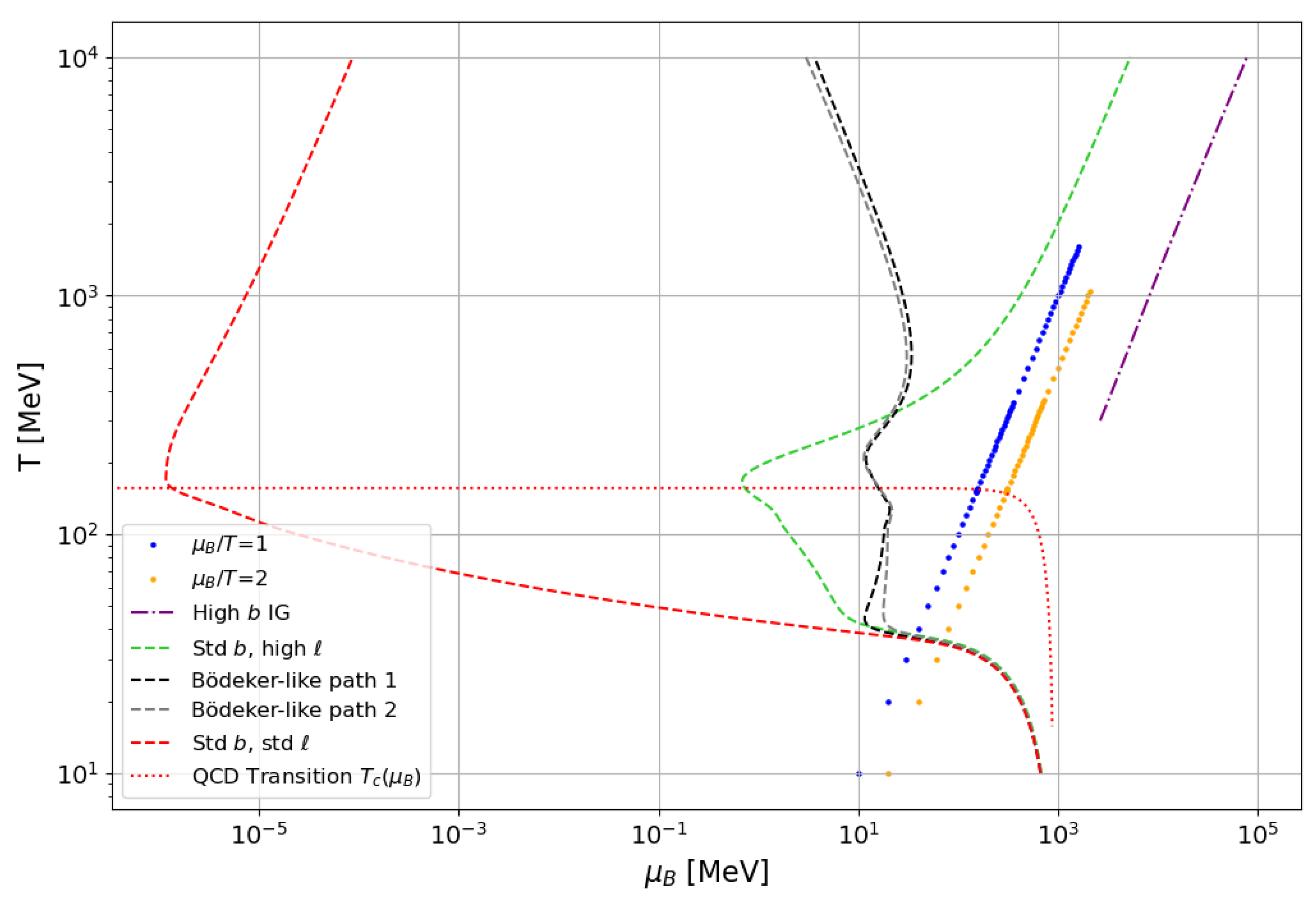
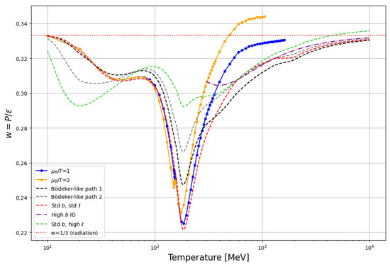
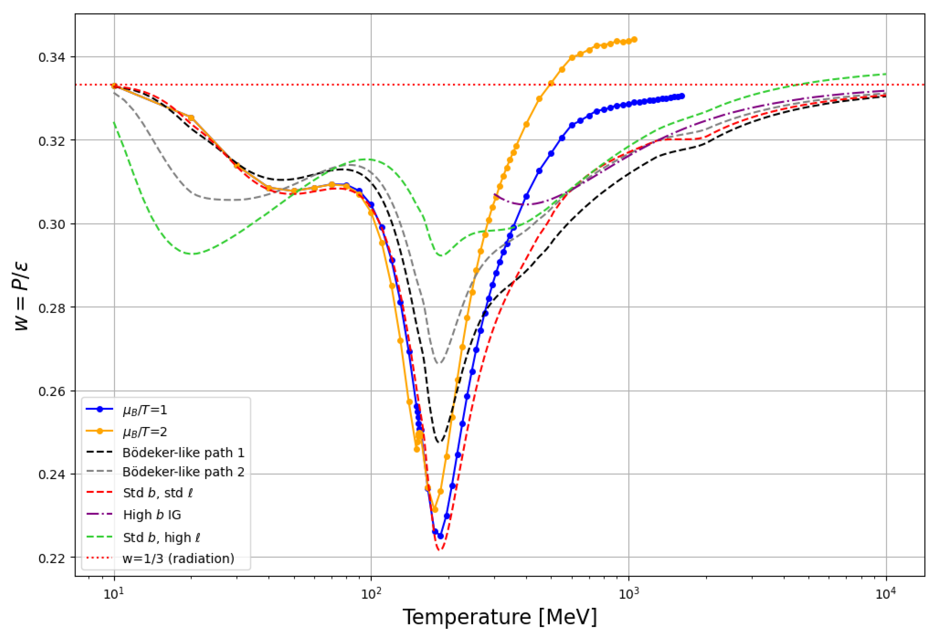
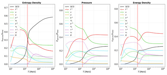
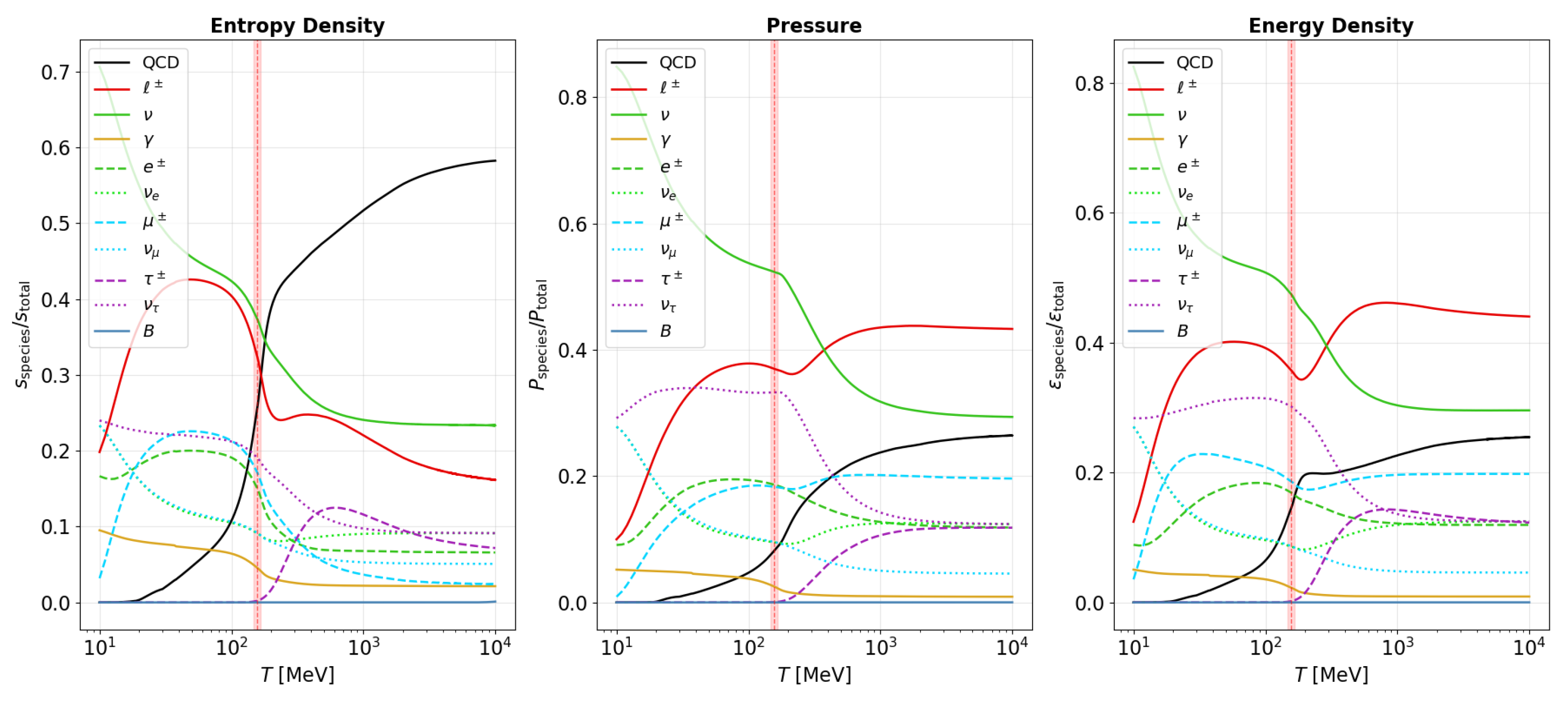
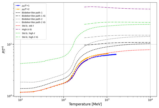
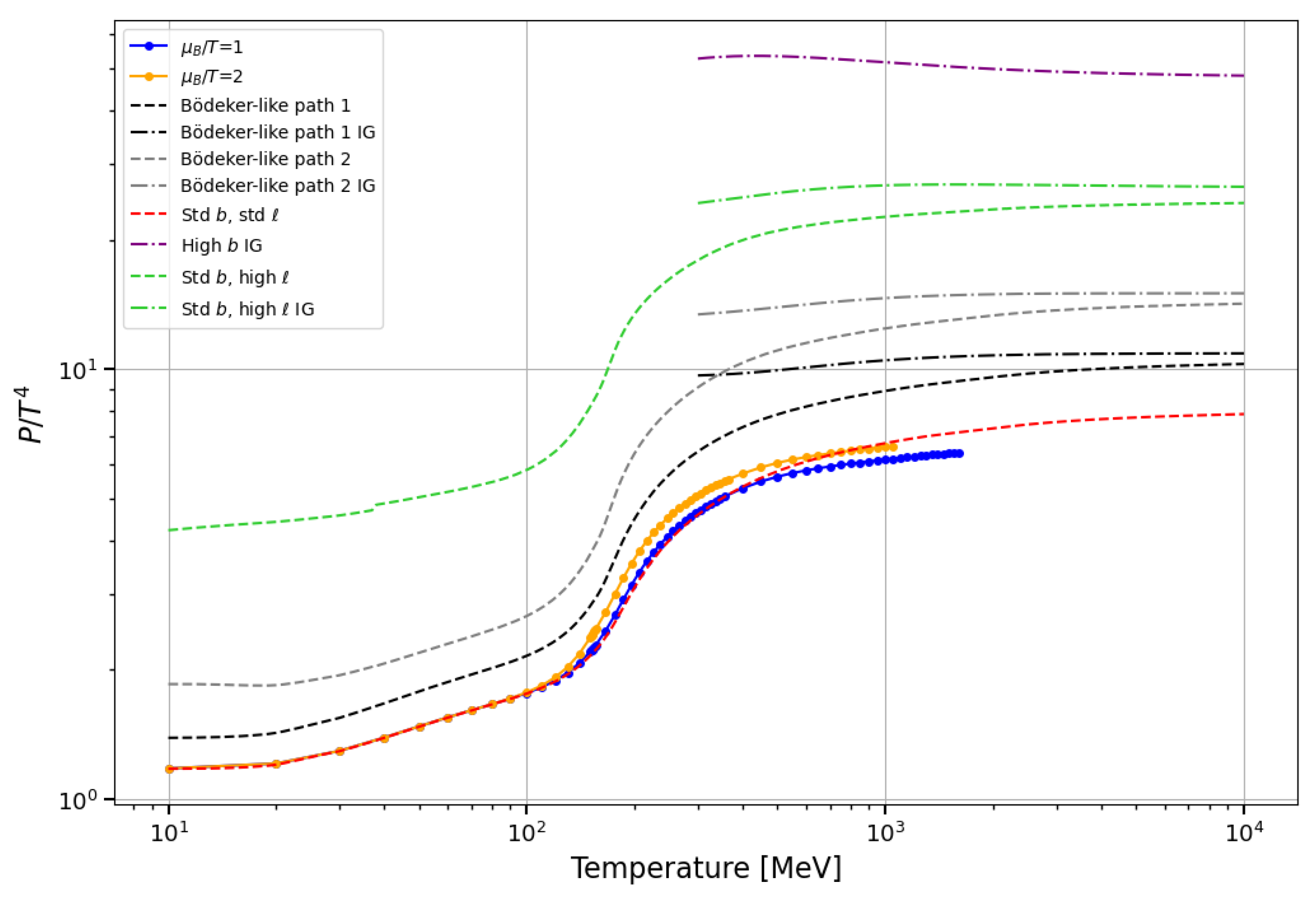
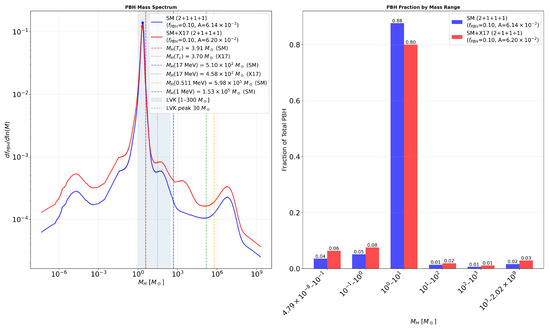
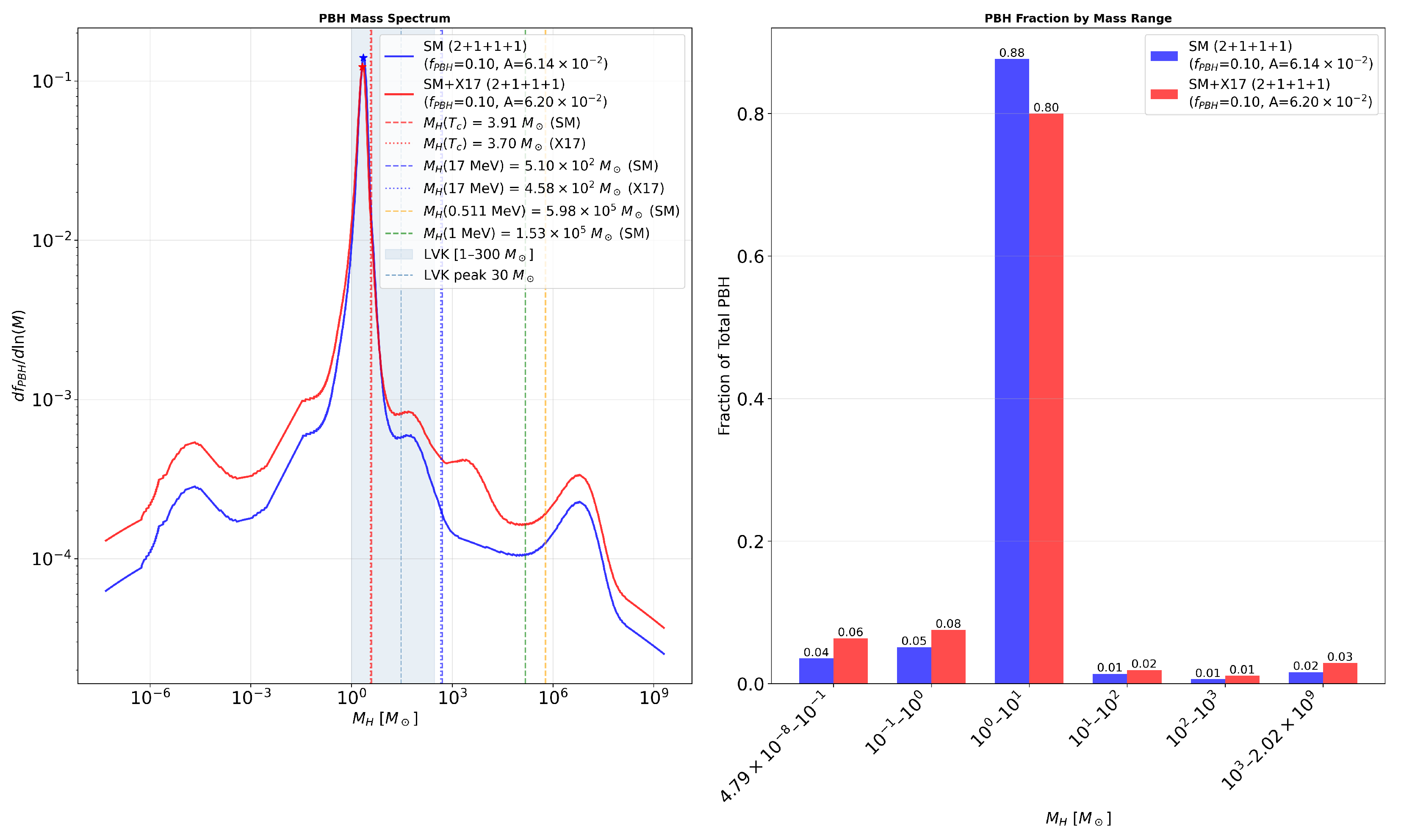
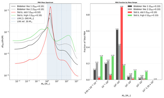
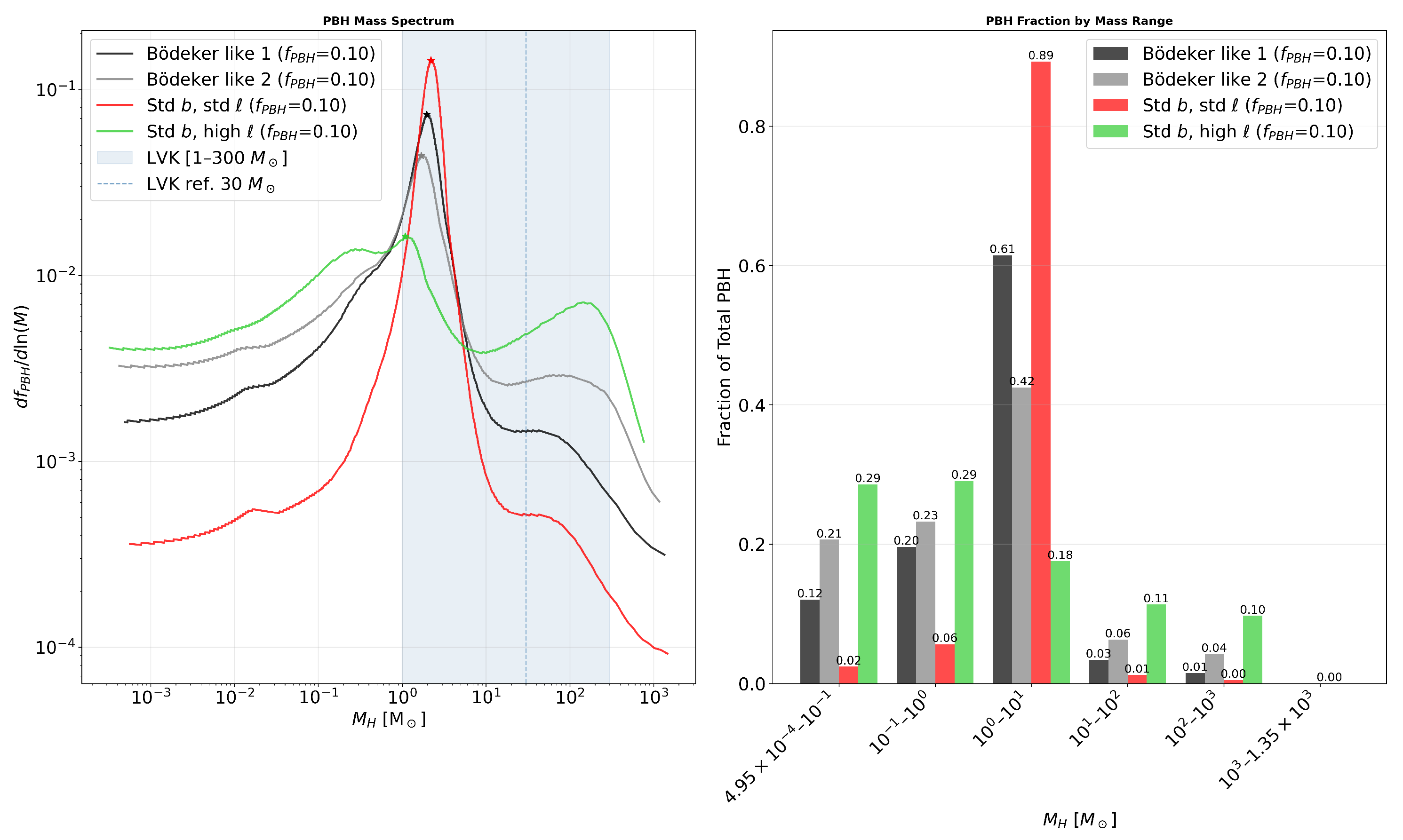
Disclaimer/Publisher’s Note: The statements, opinions and data contained in all publications are solely those of the individual author(s) and contributor(s) and not of MDPI and/or the editor(s). MDPI and/or the editor(s) disclaim responsibility for any injury to people or property resulting from any ideas, methods, instructions or products referred to in the content. |
© 2026 by the authors. Licensee MDPI, Basel, Switzerland. This article is an open access article distributed under the terms and conditions of the Creative Commons Attribution (CC BY) license.