Global Near-Real-Time Burned Area Mapping Using Sentinel-2 and VIIRS Active Fires

Abstract

Despite the well-known strong influence of spatial resolution on the quality of burned area mapping and the need for timely environmental information, global wildfire monitoring services are commonly based on coarse spatial resolution (300–500 m) reflectance imagery and deliver products months or years after the present date. The paper presents, for the first time, an algorithm that provides highly accurate near-real-time medium spatial resolution burned area, from 20 m Sentinel-2 imagery. The paper exploits a pioneering sensor-independent potential of a mapping method, based on land surface reflectance modelling and machine learning, originally optimised for Sentinel-3 imagery. The mapping method uses predictions of time series of burned area from a neural network, which are combined with the spatio-temporal density of active fire detections. The mapping method was calibrated and validated using reference datasets for the years 2020 and 2019, respectively. The novelty of this method lies in its high accuracy and multi-latency flexibility: it achieves a Dice coefficient (DC) of 82.7% with zero-day latency, already surpassing the 81.8% accuracy of current state-of-the-art non-time critical methods. As reflectance data availability increases, accuracy scales to DC 84.7% and 85.4% with 5 and 10 days of latency, respectively, and to DC 87.2% for monthly composites with 45 days of latency.

1. Introduction

The frequency and intensity of extreme wildfires are increasing due to anthropogenic global warming [1,2], leading to longer fire seasons and worsened environmental and socio-economic impacts [3,4]. Therefore, precise, timely information about the areas affected by fires is becoming critical for evaluating the environmental and societal impacts of fires [5]. Burned area (BA) is identified as one of the Essential Climate Variables by the Global Climate Observing System (GCOS) programme [6], as it is critical, for example, in the estimation of the amount of gas and particulate matter released by fires [7,8,9].

Several wildfire monitoring services already provide BA data at a global scale. However, the BA datasets are generated at coarse spatial resolutions (300–500 m). They are often distributed several months or years after the present date on a so-called non-time critical (NTC) basis. For example, the US National Aeronautics and Space Agency (NASA) provides the 500 m MCD64A1 product [10] with a latency of several months. The Copernicus Climate Change Service and the European Space Agency’s Climate Change Initiative (CCI) Fire Disturbance project distribute the 300 m CS3BA11 and FIRECCIS311 products, respectively, with a latency of several years [11,12,13]. The Copernicus Land Monitoring Service (CLMS) is the only exception, as it provides a 300 m product, the CLMBA40nrt, on a near-real-time (NRT) basis, the day after image sensing, and, since recently, at a similar accuracy to the above-mentioned NTC products [14].

Several studies have demonstrated that the quality of BA maps depends strongly on the spatial resolution of input imagery. In particular, medium spatial resolution imagery (20–30 m), from Sentinel-2 and Landsat, leads to large improvements in accuracy due to an improvement in the detection of small fires [15,16], which have considerable implications in the evaluation of fire impacts. Ramo et al. [17] found that using 20 m Sentinel-2 BA estimates instead of 500 m MODIS estimates increased fire emission estimates by 31–101% in sub-Saharan Africa. For this reason, several methods have been developed to provide medium-resolution BA products, but not yet at the global scale.

Semi-automated methods have been used, for example, by the Portuguese Forest Research Centre to provide BA products for Portugal since 1975 [18] or by the Queensland Government between 1986 and 2016 for the state of Queensland in Australia [19,20]. Such methods might yield high-quality BA data, but their reliance on human intervention hinders their implementation at regional or global scales.

Fully automated methods have been used to retrieve BA; however, they have not yet been developed for an NRT basis at a global scale. The United States Geological Survey provides BA data from 1984 onwards for the Conterminous United States, using an algorithm that provides NRT estimates based on temporal mosaics before the mapping day [21]. Roteta et al. [15] also designed an algorithm that provides NRT estimates based on image pairs, but it was also designed for a specific region, sub-Saharan Africa in this case. Furthermore, successive evolutions of this algorithm [22,23] incorporated images acquired after the mapping day, thereby losing the capacity to provide NRT estimates. Roy et al. [16] designed an algorithm to simultaneously use Landsat and Sentinel-2 data by analysing image pairs; in this case, three months of data were needed to map the central month. Long et al. [24] and Bastarrika et al. [22] designed two algorithms to map BA at a global scale, but both used temporal mosaics of reference data before and after the mapping days, rendering those approaches unsuitable for NRT estimates.

The challenge of global BA mapping is the broad diversity of soil reflectivity and fire-related spectral changes across the globe [19,25]. NRT mapping adds the challenge of limited observational data availability, as observations after the mapping day are unavailable. Time series of observations after the mapping day are useful for distinguishing between land surface reflectance changes caused by fire, which persist over time, and ephemeral reflectance changes unrelated to fire, such as shadows cast by clouds. The most recent NRT BA mapping studies propose using temporal or spatio-temporal deep learning models, such as recurrent neural networks or Transformer-based models, possibly because they may be more efficient at exploiting the temporal information embedded in reflectance time series than temporal mosaics or image-pair analyses previously used. However, deep learning needs large amounts of data. For this reason, some studies proposed addressing such data needs by using other global or regional products as training data [26,27,28]. Such practice inevitably limits the algorithm’s output accuracy to that of existing products. Nolde et al. [29] proposed an NRT mapping method for medium- to coarse-resolution (10–500 m) data using a superpixel-based image segmentation technique, temporal mosaics, and a graph-based deep learning model. However, the intermediate accuracy of their output estimates, similar to that of the coarse-resolution 500 m MCD64A1 product [29,30], possibly reflected an inefficient use of temporal reflectance information.

Land surface reflectance modelling of fire effects on vegetation [31,32] has been applied over a relatively large area in southern Africa to map BA using Landsat and Sentinel-2 imagery and machine learning [16]. Building on those methods, Padilla et al. [14] developed an algorithm that implements fire effect modelling and deep learning specifically designed to exploit the temporal evolution of 300 m Sentinel-3 reflectance data, yielding unprecedented accuracy and timeliness in BA estimates. Therefore, the purpose of this study is to demonstrate the suitability of this algorithm for NRT BA mapping from medium-resolution 20 m Sentinel-2 data.

The proposed algorithm can retrieve BA estimates in NRT and on an NTC basis. It is based on a deep learning algorithm trained on a dataset automatically built from a global sample of reflectance time series located at active fire detections. A physically based radiative transfer modelling framework is used to estimate land surface fire effects independently for each time series, thereby building a swarm of quantifications of fire effects, each with an associated spectral evolution. Fractional estimates of fire-affected area predicted by the deep learning model are combined with the spatio-temporal density of active fire detections to reduce false positives. This combination is calibrated using time series of Landsat-derived reference data generated in 2020 by the Copernicus Climate Change Service (C3S). The main output of the algorithm is the date of the BA detection, which was validated against independent C3S reference data from the previous year, 2019. The validation year was selected to enable comparison with the Bastarrika et al. [22] global 20 m BA algorithm, which was also validated using the same 2019 dataset. At the time the calibration analysis started, the archive of Sentinel-2 Level-2A product files was complete for 2020, but not for 2017–2018, which led to the selection of 2020 as the calibration year. The validation results are contextualised by including other operational global products available for 2019 at the time of writing this manuscript: the NTC CLMBA40ntc CLMS product, the MCD64A1 Collection 6 from the United States NASA, the C3SBA11 from C3S, and the FIRECCIS11 from the CCI Fire Disturbance project. The Global Annual Burned Area Map (GABAM) from Long et al. [24] is available for 2019 but is not included in the validation analysis due to its large temporal mismatches with the reference data (one-year temporal resolution vs. up to 48 days).

2. Methods

2.1. Burned Area Mapping

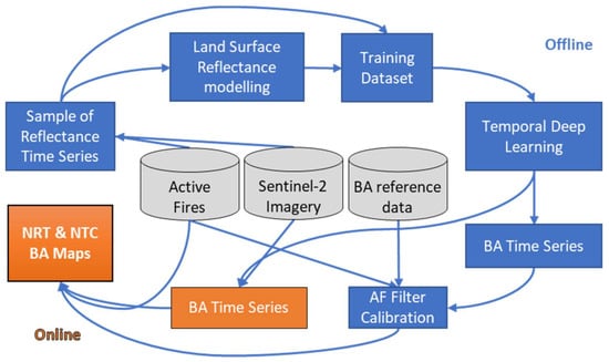
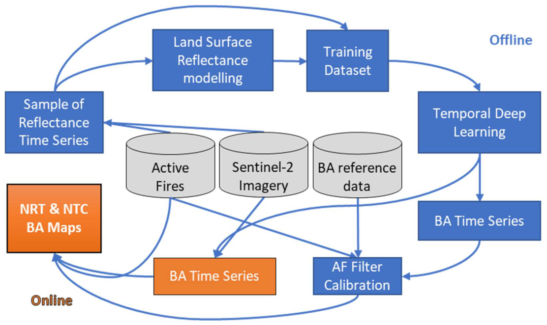
The burned area algorithm used here was developed in the framework of the Copernicus Land Monitoring Service and was originally designed to process Sentinel-3 OLCI&SLSTR imagery. A detailed description of the algorithm can be found in the open access manuscript by Padilla et al. [14]. Therefore, this section includes a summary of the algorithm (Figure 1), its calibration, and the adaptations needed for its use with Sentinel-2 imagery.

Figure 1. The burned area mapping algorithm workflow. The calibration steps (blue boxes) run once, global and offline, and prepare the algorithm to be run in the operational processing chain (orange boxes). The arrows indicate the data flow, which starts at the input data (grey boxes).

2.1.1. Algorithm Overview

The deep learning algorithm consists of a neural network (NN) formed by convolutional layers [33] followed by a Long Short-Term Memory (LSTM) layer [34], a recurrent neural network designed to process the time series of data. The convolutional layers are applied to the spectral and temporal dimensions of the data. Therefore, the NN is applied on a per-pixel basis. The network is trained on a global, automatically built dataset containing time series of reflectance observations and associated fractional BA derived from physically based radiative transfer modelling. Fractional BA is estimated by a spectral mixing model of land surface changes caused by fire effects over vegetation [31,32], and taking into account the effects of land surface anisotropy [35,36] on the Sentinel-2 reflectance measurements. A logistic model is used to combine the fractional BA predicted by the NN with the spatio-temporal density of active fire detections. This combination aims at reducing false positive detections—land surface changes unrelated to fires, such as agricultural practices, fast vegetation senescence or cloud shadows. The generation of the global dataset with reflectance time series, and the NN training and the logistic model calibration analyses are performed once, globally and ‘offline’, outside the processing chain.

The NRT implementation of the algorithm produces one BA map per day (hereinafter referred to as BAS2nrtR0) using reflectance data for that day and the previous 45 days. Additionally, each daily NRT map is updated twice over the following ten days: BAS2nrt0, generated at day zero, is updated in days five (BAS2nrtR5) and ten (BAS2nrtR10), in both cases with all images available until the product generation day. Accuracy is expected to improve with each update, as additional images after the mapping day are expected to reduce errors, such as false positives due to cloud shadows, caused by the scarcity of observations. Lastly, an NTC monthly BA map (BAS2ntc) is produced using all available images for that month and the previous and posterior 45 days. Therefore, BAS2ntc is expected to have the highest accuracy.

2.1.2. Input Data

The BA mapping is mainly based on Sentinel-2 MultiSpectral Instrument (MSI) Level-2A data from the European Space Agency (ESA). The Sentinel-2 mission consists of a constellation of two satellites in the same sun-synchronous orbit (https://sentinels.copernicus.eu/copernicus/sentinel-2, accessed on 28 April 2026). The Level-2A product provides land surface reflectance estimates and a Scene Classification Layer (SCL) that includes information on its quality and land surface type [37]. The MSI swath of 290 km and the two satellites allow a revisit time of 5 days at the equator and 2–3 days at mid-latitudes. The BA algorithm uses five of the 20 m spectral bands: the red band B4, centred at 0.665 µm, two near-infrared (NIR) bands B6 and B8A, centred at 0.740 and 0.864 µm, respectively, and two shortwave infrared (SWIR) bands B11 and B12, centred at 1.610 and 2.190 µm, respectively. Similar to Roteta et al. [15], MSI reflectances are discarded if classified as ‘no-data’, ‘saturated or defective pixel’, ‘cloud shadows’, ‘cloud medium probability’, ‘cloud high probability’, ‘thin cirrus’ or ‘snow or ice’, or if B12 reflectance is below 0.07.

The BA mapping is also based on active fire data from NASA’s 375 m VIIRS active fire and thermal anomalies products [38]. The NRT VNP14IMGTDL VIIRS active fire product is used for the NRT BA processing chain, and the NTC VIIRS VNP14IMGML product for the NTC BA processing. The two active fire products are available at the LANCE archive via HTTP [39] and through the Archive Download tool of the Fire Information for Resource Management System [40], respectively. They provide the spatial location, timing, and degree of confidence for the fire detection. Only detections labelled as ‘vegetation fire’ are used by the algorithm, and those detected over urban areas are excluded, as they may correspond to heat released by industrial buildings [41,42]. Pixels over urban areas are identified using the Land Cover (LC) v2.1.1 product from the Copernicus Climate Change Service [43].

2.1.3. Training Data

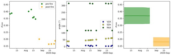
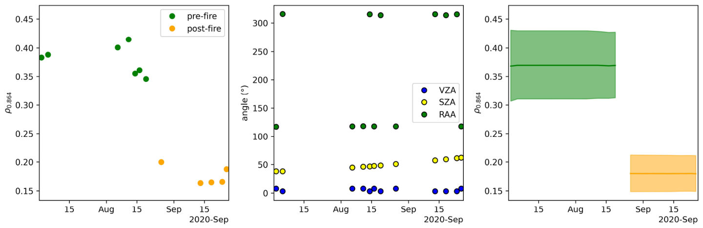
The training data are built from a global sample of reflectance time series and associated estimates of the fractional area of a pixel affected by fire (${0\le f}_{\mathrm{b}}\le 1$), retrieved independently for each time series using two semi-empirical models. The details of the semi-empirical modelling can be found in Padilla et al. [14]. In summary, a linear spectral mixing model [31,32] is used to estimate $f_{\mathrm{b}}$ and its associated uncertainty from two consecutive land surface reflectance estimates at a common acquisition geometry (Figure 2 and Figure 3). The model assumes that the reflectance of the land surface unaffected by the fire is constant over short time intervals between consecutive observation times. Reflectance at the common acquisition geometry at the observation times immediately before and after the active fire detection times is retrieved from a semi-empirical bidirectional reflectance model [35,36], independently applied over the two segments of the reflectance time series before and after the active fire detection time. The two semi-empirical models are based on linear equations; therefore, the model parameters (expected values and associated uncertainties) are estimated using least-squares estimators. Time series are discarded if (1) spectral model parameter expected values are outside the ranges with physical meaning or (2) the highest $f_{\mathrm{b}}$ expected value is found at an observation time not immediately after active fire detection time, which helps avoid using time series with invalid data or without burns, eventually sampled by false active fire detections or due to misalignments between the 375 m VIIRS and the 20 m Sentinel-2 pixels.

Figure 2. Illustration of the semi-empirical modelling for a time series of Sentinel-2 MSI NIR band B8A reflectance observations (at wavelength 0.864 µm; ${\rho }_{0.864}$) at an active fire detected in the Asian Boreal Forest in August 2020. The left panel shows the reflectance observations before (green) and after (orange) the active fire detection time. The middle panel shows the acquisition geometry angles: viewing zenith angle (VZA), solar zenith angle (SZA) and relative azimuth angle (RAA). The right panel shows the estimated NIR reflectance before (green) and after (orange) the active fire detection time, normalised to a common acquisition geometry. The solid lines represent the expected values, and the shaded areas the 95% confidence intervals.

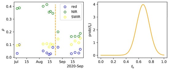
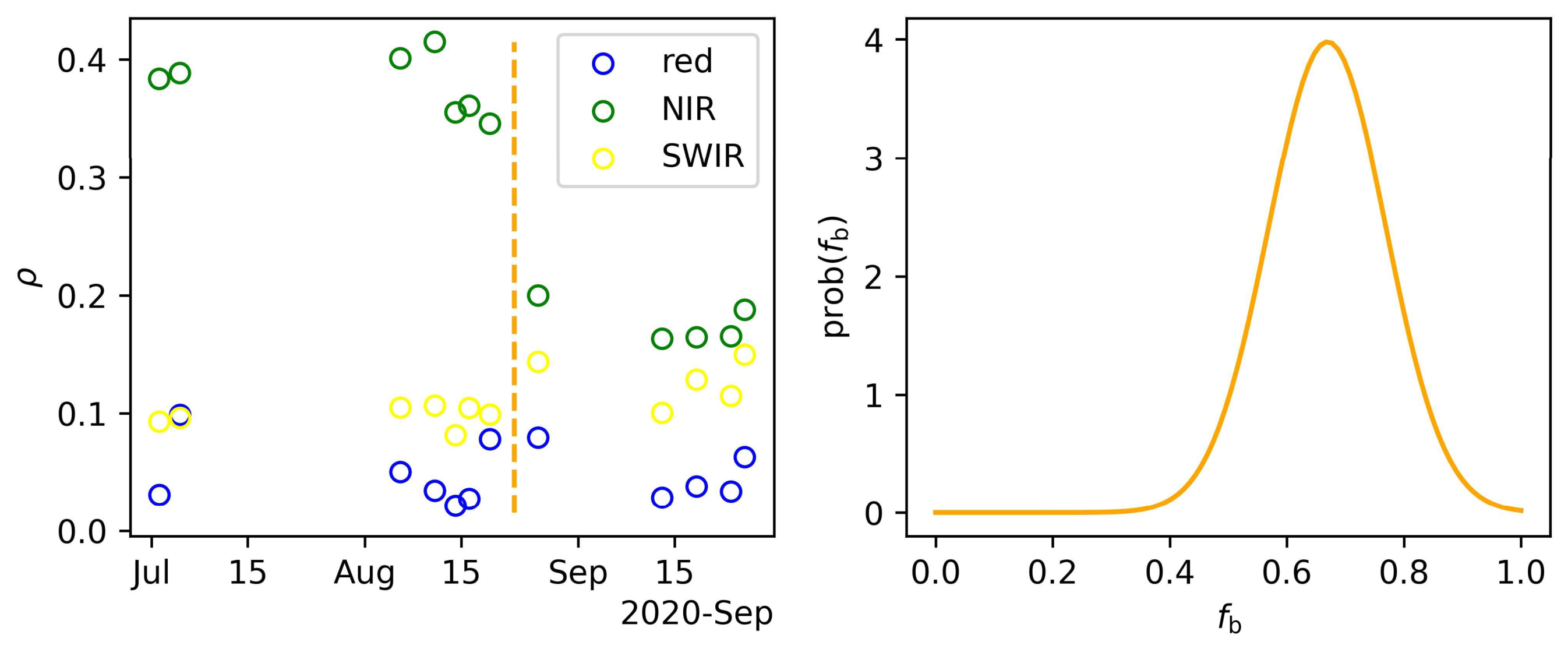
Figure 3. Illustration of Sentinel-2 MSI red, NIR and SWIR observations (bands B4, B8A and B12, respectively; left panel) for the same time series shown in Figure 2, with the associated active fire detection (dashed orange vertical line), and the probability density function of the fraction of fire-affected material $f_b$ retrieved by the semi-empirical modelling (right panel).

The target data to be predicted by the neural network can be represented as a matrix, $\mathbf{Y}$, with $t_{\mathrm{m}\mathrm{a}\mathrm{x}}$ columns and two rows: one for each target variable, $f_{\mathrm{b}}$, and one for the probability that $f_{\mathrm{b}}$ is above 0.1, ${\mathrm{p}\mathrm{r}\mathrm{o}\mathrm{b}(f}_{\mathrm{b}}>0.1)$. $t_{\mathrm{m}\mathrm{a}\mathrm{x}}$ represents the number of observations included in a time series. The variable ${\mathrm{p}\mathrm{r}\mathrm{o}\mathrm{b}(f}_{\mathrm{b}}>0.1)$ allows incorporating the uncertainty of the semi-empirical modelling into the following steps of the BA algorithm. $f_{\mathrm{b}}$ and ${\mathrm{p}\mathrm{r}\mathrm{o}\mathrm{b}(f}_{\mathrm{b}}>0.1)$ range from zero to one and are zero except for the first observation after the active fire detection time.

$$\mathbf{Y}=\left[\begin{array}{cccc}{f}_{\mathrm{b},1}& f_{\mathrm{b},2}& \dots & f_{\mathrm{b},{\mathrm{t}}_{\mathrm{m}\mathrm{a}\mathrm{x}}}\\ {{\mathrm{p}\mathrm{r}\mathrm{o}\mathrm{b}(f}_{\mathrm{b}}>0.1)}_1& {{\mathrm{p}\mathrm{r}\mathrm{o}\mathrm{b}(f}_{\mathrm{b}}>0.1)}_2& \dots & {{\mathrm{p}\mathrm{r}\mathrm{o}\mathrm{b}(f}_{\mathrm{b}}>0.1)}_{t_{\mathrm{m}\mathrm{a}\mathrm{x}}}\end{array}\right]$$

(1)

Each reflectance time series can be represented by another matrix, $\mathbf{X}$, with $t_{\mathrm{m}\mathrm{a}\mathrm{x}}$ columns and five rows, one for each predictor variable: three spectral bands B4, B8A and B12, in the red, NIR and SWIR regions, respectively, and two spectral indices, the Normalised Difference Vegetation Index (NDVI) and the Normalised Burn Ratio Index 2 (NBR2) [44]. Spectral changes in the red, NIR, and SWIR spectral regions are strongly related to changes in leaves’ chlorophyll content and structure, canopy cover and landscape dryness [45]. Spectral indices are commonly used for burned area mapping because they are less affected by variations in image acquisition geometry than raw reflectance observations. NBR2 is often used in global burned algorithms [13,22], and NDVI has been found useful for reducing false positives (incorrect burned detections) associated with agricultural harvesting [46].

$$\mathbf{X}=\left[\begin{array}{cccc}{\mathsf{\rho }}_{red,1}& {\mathsf{\rho }}_{red,2}& \dots & {\mathsf{\rho }}_{red,t_{\mathrm{m}\mathrm{a}\mathrm{x}}}\\ {\mathsf{\rho }}_{NIR,1}& {\mathsf{\rho }}_{NIR,2}& \dots & {\mathsf{\rho }}_{NIR,t_{\mathrm{m}\mathrm{a}\mathrm{x}}}\\ {\mathsf{\rho }}_{\mathrm{S}\mathrm{W}\mathrm{I}\mathrm{R},1}& {\mathsf{\rho }}_{\mathrm{S}\mathrm{W}\mathrm{I}\mathrm{R},2}& \dots & {\mathsf{\rho }}_{\mathrm{S}\mathrm{W}\mathrm{I}\mathrm{R},t_{\mathrm{m}\mathrm{a}\mathrm{x}}}\\ {\mathrm{N}\mathrm{D}\mathrm{V}\mathrm{I}}_1& {\mathrm{N}\mathrm{D}\mathrm{V}\mathrm{I}}_2& \dots & {\mathrm{N}\mathrm{D}\mathrm{V}\mathrm{I}}_{t_{\mathrm{m}\mathrm{a}\mathrm{x}}}\\ {\mathrm{N}\mathrm{B}\mathrm{R}2}_1& {\mathrm{N}\mathrm{B}\mathrm{R}2}_2& \dots & {\mathrm{N}\mathrm{B}\mathrm{R}2}_{t_{\mathrm{m}\mathrm{a}\mathrm{x}}}\end{array}\right]$$

(2)

Preliminary tests showed that the best performance was observed with NN predictions from data of the same temporal length as the training data, particularly for short time series. Therefore, multiple training sets were generated across several time series lengths, with $t_{\mathrm{m}\mathrm{a}\mathrm{x}}$ ranging from 3 to 20. Each set of training data is divided into three (sub)datasets, the training, validation and testing datasets, containing, respectively, 58,485, 12,938 and 10,385 burned samples (i.e., time series with an associated active fire detection), and the same number of unburned samples, located far away from fire detections. It is important to emphasise that, here, the term ‘validation’ follows the machine learning naming convention to refer to an intermediate model assessment, not to be mistaken for the products’ independent validation analyses presented in Section 2.2.

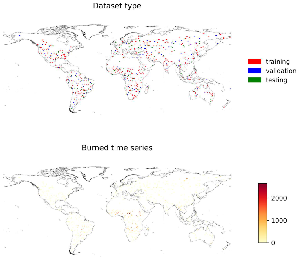
A cluster sampling design is followed to sample reflectance time series across the globe in 2020. The clusters are defined spatially by the delineations of the 100 km × 100 km Sentinel-2 tiles and temporally by calendar months. In total, 627 tiles are randomly selected across the globe: 60% (375) for training, 20% (126) for validation and 20% (126) for testing the model (Figure 4). For each selected tile, time series are sampled at 12 clusters (one per month) within a 40 km × 40 km spatial window, each located at the centre of the tile. In order to address the class imbalance problem—in our case, the high prevalence of unburned area—on each selected cluster, the same number of burned and unburned time series are sampled: up to 10,000 reflectance time series are sampled at the locations of the VIIRS active fire detections, and up to the same number of time series are sampled at locations far away from fire detections, further than 20 km and 40 days from any fire.

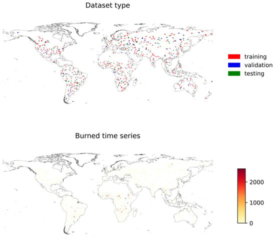
Figure 4. Spatial distribution of the units used to sample the reflectance time series for the training, validation and testing datasets (top panel) and number of reflectance time series at VIIRS active fires (up to 2642 per unit; bottom panel). For brevity, the number of unburned time series is not plotted.

2.1.4. Neural Network Training

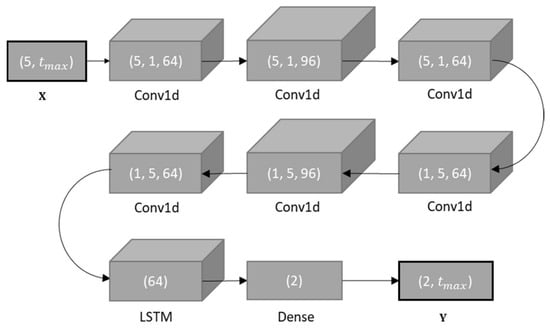
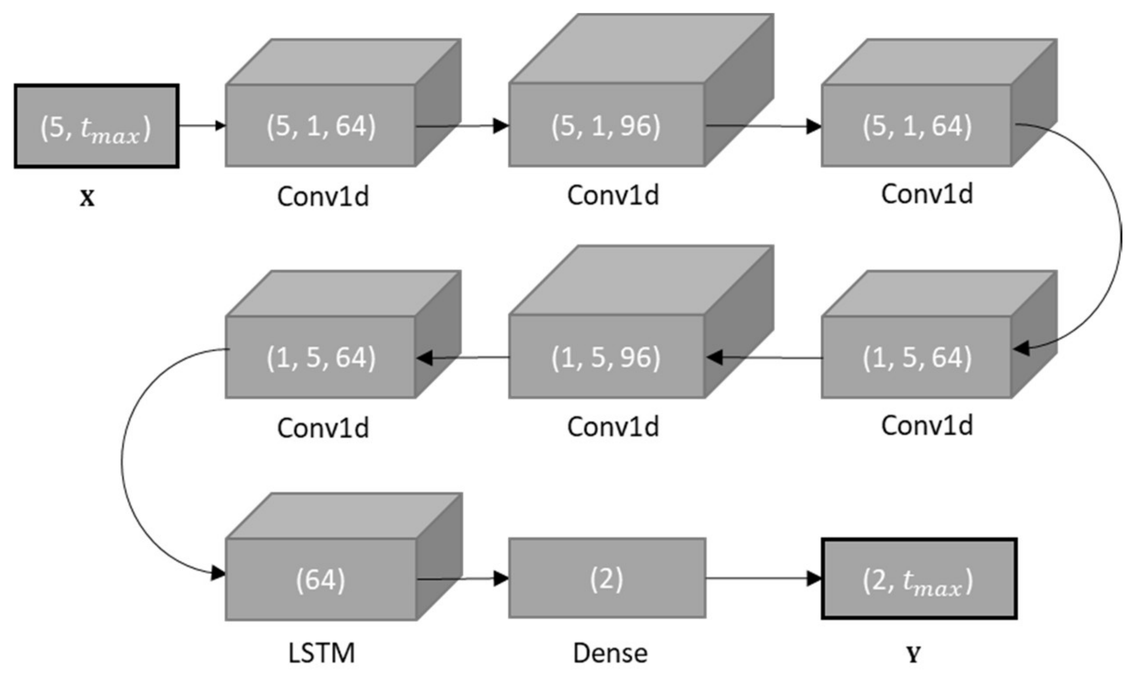
The neural network contains two blocks of 1-dimensional (1D) convolutional layers followed by a bidirectional Long Short-Term Memory (LSTM) [34] layer (Figure 5). The convolutions are applied to the spectral and temporal dimensions of the data. As recommended by De Fauw et al. [47], two blocks of 1D convolutional layers are used instead of 2-dimensional convolutional layers, leading to a smaller and faster network with similar accuracies: three 1D convolutional layers applied on the spectral dimension, with 64, 96 and 64 filters respectively and a kernel size of five, are followed by the other three 1D layers, with the same number of filters, 64, 96 and 64 filters respectively, applied on the temporal dimension with kernel size of five or up the length of the time series if that is lower than five (Table 1). The convolutional layers are followed by an LSTM layer with 64 filters and a fully connected layer, the latter activated with the sigmoid function to ensure a meaningful output range of 0 to 1. The other layers are activated by a linear function, and a dropout of 0.2 is applied in each layer. The weights and biases of the activation functions are initialised with the Glorot uniform method [48], the default method in the software used: TensorFlow [49] version 2.13.0.

Figure 5. Diagram of the neural network’s architecture designed for time series with five or more observations ($t_{\mathrm{m}\mathrm{a}\mathrm{x}}\ge 5$). For shorter time series, only the kernel dimension of the temporal convolution differs (see main text for details). The numbers within brackets represent the shapes of the input and output data ($\mathbf{X}$ and $\mathbf{Y}$), the sizes of the kernels and the number of filters used for the convolutional layers (Conv1d; the first three Conv1d layers for the spectral dimension and the following three for the temporal dimension) or the number of filters used for the Long Short-Term Memory (LSTM) and the fully connected dense layers (Dense). All layers are activated by a linear function, except the last one (Dense), which is activated by the sigmoid function, with dropout of 0.2 in all cases.

Table 1. Summary of the neural network’s hyperparameters.

Name	Values
Temporal convolutional kernel size	5
Filters of the convolutional layers	64, 96 and 64
Filters of the LSTM layer	64
Activation functions	Linear; sigmoid for the last layer
Dropout	0.2
Weights and biases initialisation	Glorot uniform method
Loss function	Mean squared error (MSE)
Stopping criteria	MSE decreases < ${10}^{-6}$ over 50 epochs
Learning rate	0.0001
Software	Tensorflow 2.13.0

One neural network is trained separately for each of the 18 sets of training data (with $t_{\mathrm{m}\mathrm{a}\mathrm{x}}$ ranging from 2 to 20). Each neural network, which contains up to 210,000 parameters, is trained by minimising the mean squared error (MSE) with Adam’s optimisation algorithm [50], with a learning rate of 0.0001 and 64 elements per batch until the MSE did not decrease by more than ${10}^{-6}$ over 50 epochs, evaluated with the validation dataset after each epoch. The network was evaluated with the testing dataset only once, after the training was finalised.

2.1.5. Burned Area Prediction

Time series of $f_{\mathrm{b}}$ and ${\mathrm{p}\mathrm{r}\mathrm{o}\mathrm{b}(f}_{\mathrm{b}}>0.1)$ maps (one for each reflectance image acquisition) are generated by the trained neural networks, covering the products’ mapping periods—i.e., a natural month for the NTC and a single day for the NRT products—and an additional 15-day buffer. Pixels located far from active fires (more than 20 km and 40 days from any fire) are flagged as unburned and excluded from the analyses, which allows a large improvement in computational speed. This computational optimisation implies a small penalty, in the form of an omission of less than 0.2% of the burned area, according to a comparison between this VIIRS-based unburned mask and 30 m Landsat-derived reference data, undertaken during the preparation of the original algorithm calibration for Sentinel-3 data [14].

The neural network prediction ${\mathrm{p}\mathrm{r}\mathrm{o}\mathrm{b}(f}_{\mathrm{b}}>0.1)$ is combined with the density of active fire detections ($\mathrm{A}\mathrm{F}\mathrm{d}\mathrm{e}\mathrm{n}\mathrm{s}\mathrm{i}\mathrm{t}\mathrm{y}$) using a logistic regression model designed to predict the probability that a pixel is classified as burned by the reference data, $\mathrm{p}\mathrm{r}\mathrm{o}\mathrm{b}\left(\mathrm{b}\right)$. Fire density is based on a Gaussian kernel with a standard deviation of 2 km and 4 days, and is temporally accumulated to match the time intervals between consecutive reflectance image acquisitions. The large kernel size in the spatial dimension (2 km) helps limit the spatial ‘mismatches’ between the 375 m VIIRS active fire detections and the 20 m Sentinel-2 reflectance observations. The $\mathrm{A}\mathrm{F}\mathrm{d}\mathrm{e}\mathrm{n}\mathrm{s}\mathrm{i}\mathrm{t}\mathrm{y}$ aggregations across the temporal dimension allow addressing the datasets’ temporal mismatches, caused by cloud coverage and the different satellite revisit frequencies: daily (VIIRS) vs every 5 days (Sentinel-2).

This logistic model is calibrated separately for the two mapping modes, NTC and NRT (at day 0), using the C3S BA reference data for 2020, which includes long time series (≥48 days) of Landsat-based BA maps across 106 units. The time series of maps of ${\mathrm{p}\mathrm{r}\mathrm{o}\mathrm{b}(f}_{\mathrm{b}}>0.1)$ and $\mathrm{A}\mathrm{F}\mathrm{d}\mathrm{e}\mathrm{n}\mathrm{s}\mathrm{i}\mathrm{t}\mathrm{y}$ (one every ~5 days) are temporally mosaicked to match the periods covered by the reference data, similarly as in the final temporal mosaics of the product (mentioned in the paragraph below) and with the $\mathrm{A}\mathrm{F}\mathrm{d}\mathrm{e}\mathrm{n}\mathrm{s}\mathrm{i}\mathrm{t}\mathrm{y}$ value of the acquisition time with the highest ${\mathrm{p}\mathrm{r}\mathrm{o}\mathrm{b}(f}_{\mathrm{b}}>0.1)$. The pixels with estimated $\mathrm{p}\mathrm{r}\mathrm{o}\mathrm{b}\left(\mathrm{b}\right)$ below a specific threshold are flagged as unburned (i.e., ${\mathrm{p}\mathrm{r}\mathrm{o}\mathrm{b}(f}_{\mathrm{b}}>0.1)=0$ and $f_{\mathrm{b}}=0$). This threshold is selected according to the output’s accuracy measured by the Dice coefficient; 21 threshold candidates were tested, from 0 to 1 with increments of 0.05, and the one leading to the highest Dice coefficient was selected as the optimal $\mathrm{p}\mathrm{r}\mathrm{o}\mathrm{b}\left(\mathrm{b}\right)$ threshold. Each dataset used to calibrate the logistic model contains 1 million observations sampled across the 106 units. The stratified random sampling design of the reference data is taken into account by allocating the sample across the units inversely proportional to the inclusion probability. Therefore, the logistic regression and the $\mathrm{p}\mathrm{r}\mathrm{o}\mathrm{b}\left(\mathrm{b}\right)$ threshold are representative of the entire globe.

The output products consist of temporal mosaics of burn dates (day of the year) detected during the mapping period: for the NTC product, a whole calendar month, and for the NRT product, a single day. The highest ${\mathrm{p}\mathrm{r}\mathrm{o}\mathrm{b}(f}_{\mathrm{b}}>0.1)$ value determines the detection date when multiple burns are detected across the product mapping period and the additional 15-day buffer. Pixels with no prediction available during the mapping period (with no observation available during the mapping period or with less than three reflectance observations during the entire mapping period and the previous and posterior 45 days) are flagged as no-data (−1).

2.2. Validation Analysis

The validation dataset was generated by the Copernicus Climate Change Service (C3S) for 2019 [51], similarly to the 2020 reference dataset used for algorithm calibration (see previous section). The dataset consists of long time series of BA maps, generated by supervised classifications of consecutive Landsat image pairs, covering approximately 100 × 100 km² squares, for a sample of 105 units distributed across the globe, following a stratified random sampling design based on the Ecoregions 2017 biomes [52]. The validation analysis for the Sentinel-2 products presented here focused on 40 × 40 km² squares centred on each sampled unit to keep the computational effort required for product generation at affordable levels. The amount of data available in each unit, commonly referred to as cluster size, affects the uncertainty but not the bias of the accuracy estimates [53]. Therefore, using the 40 × 40 km² cluster instead of the 100 × 100 km² cluster might increase the standard errors of the accuracy estimates, but it is not expected to introduce any bias. The accuracy measures are derived from error matrices generated by a cross-tabulation analysis, as is common in BA products [54]. Accuracy inferences consist of a stratified combined ratio estimator [55], which accounts for the amount of available data in each sampling unit. Similarly as in Padilla et al. [14,56], product pixels with no-data are considered as no-data and accuracy measures are defined as ratios: (1) the Dice coefficient (DC) [56], the conditional probability that one classifier identifies a pixel as burned, given that the other classifier also identified it as burned, (2) the commission error ratio (Ce), the amount of commission errors divided by the total product BA, (3) the omission error ratio (Oe), the amount of omission errors divided by the total reference BA, and (4) the relative bias (relB), the difference between the product and reference BA divided by the reference BA.

3. Results

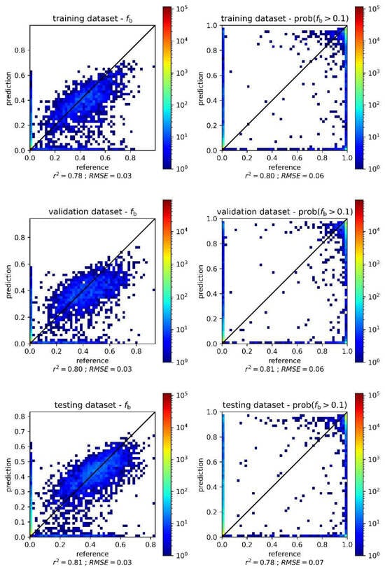
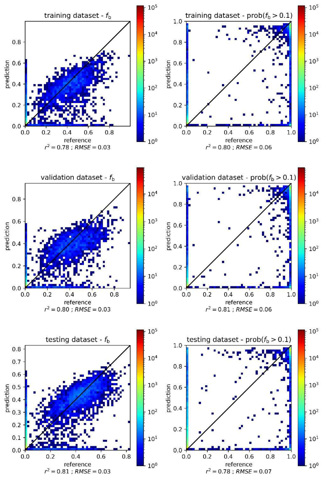
The observed NN training performances are relatively high. The highest performance is observed at the longest time series ($t_{\mathrm{m}\mathrm{a}\mathrm{x}}=20$): similarly across the three evaluation datasets, training, validation and testing, the correlation coefficient ($r^2$) and root mean squared error (RMSE) for the fractional BA ($f_{\mathrm{b}}$) are approximately 0.8 and 0.03, respectively; for ${\mathrm{p}\mathrm{r}\mathrm{o}\mathrm{b}(f}_{\mathrm{b}}>0.1)$, 0.79 and 0.07, respectively (Figure 6). The observed training performance declines with time series length, leading to the lowest RMSE of approximately 0.08 and 0.15 for $f_{\mathrm{b}}$ and ${\mathrm{p}\mathrm{r}\mathrm{o}\mathrm{b}(f}_{\mathrm{b}}>0.1)$, respectively, at the shortest time series ($t_{\mathrm{m}\mathrm{a}\mathrm{x}}=3$).

Figure 6. Scatter plots between NN predictions and reference data (inferences from semi-empirical modelling) for the two target variables ($f_{\mathrm{b}}$ and ${\mathrm{p}\mathrm{r}\mathrm{o}\mathrm{b}(f}_{\mathrm{b}}>0.1)$), in the training, validation and testing datasets (top, middle and bottom panels, respectively) with the time series of 20 observations. The density of points is represented by the colour palette. The solid black line represents the 1:1 line.

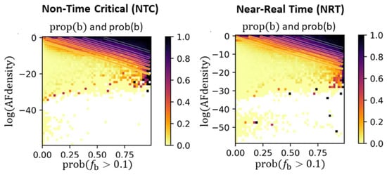
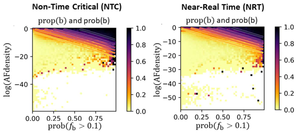
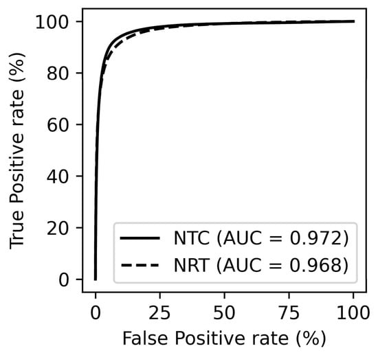
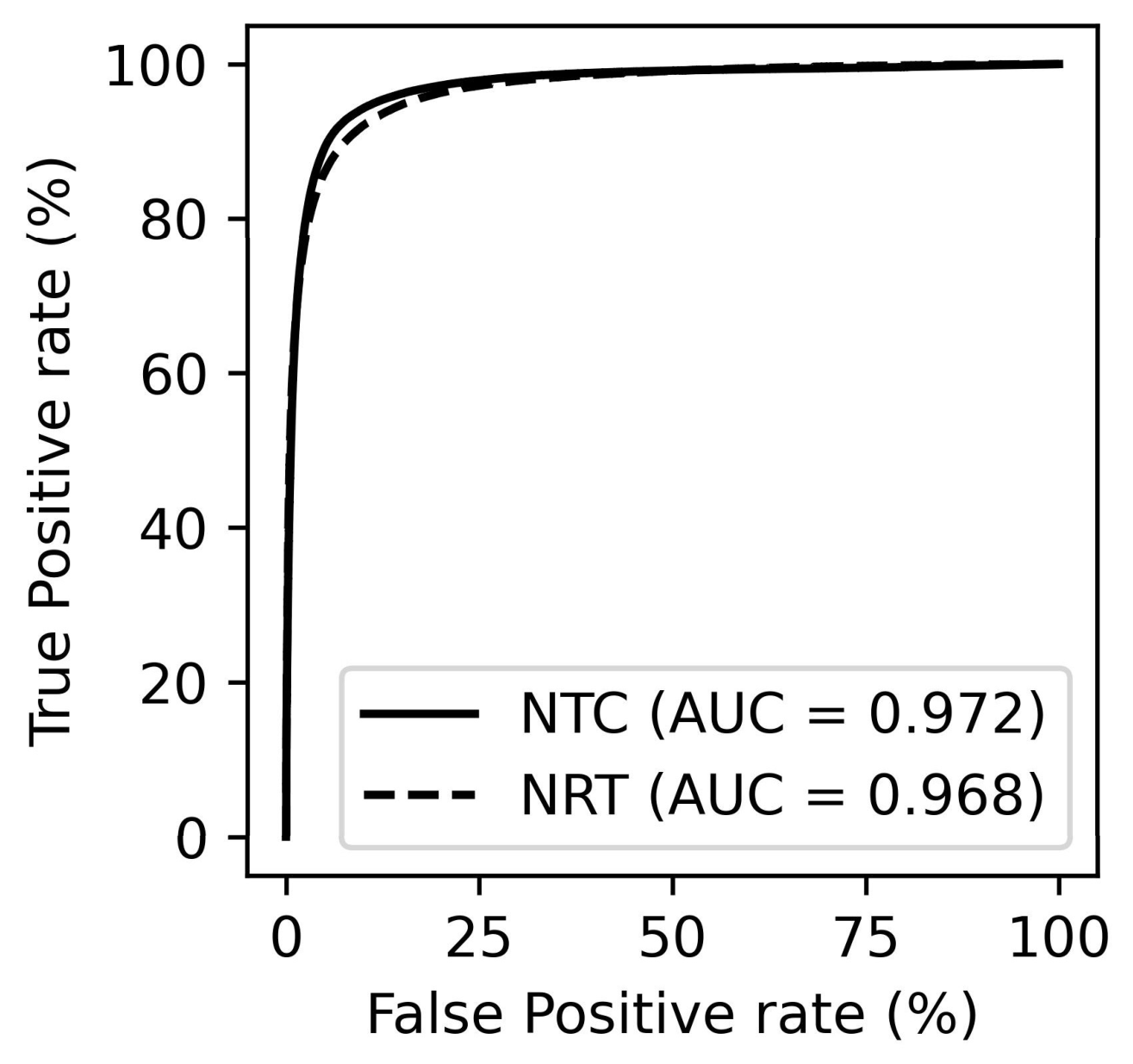
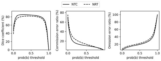
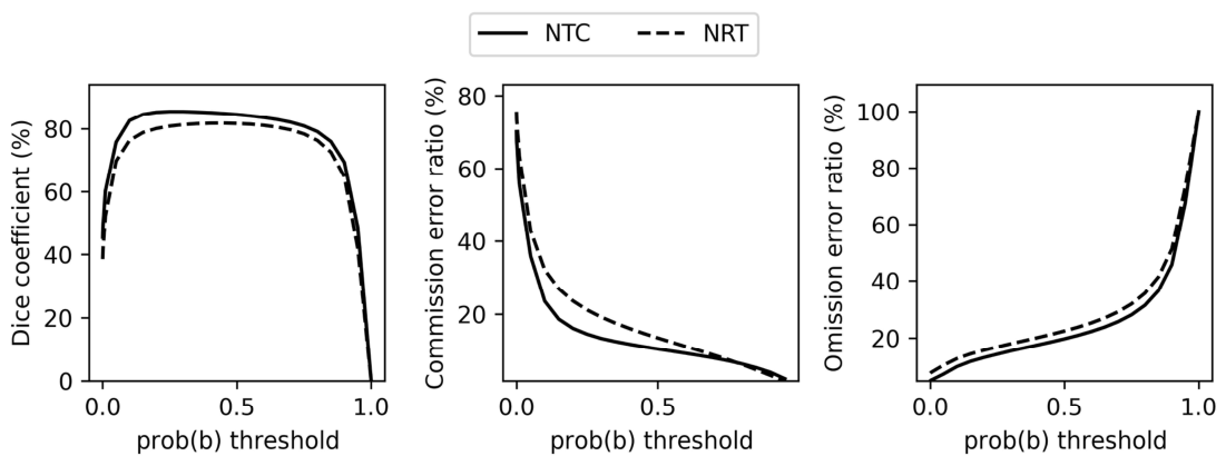
The distribution of reference burned classifications across the two-dimensional space of ${\mathrm{p}\mathrm{r}\mathrm{o}\mathrm{b}(f}_{\mathrm{b}}>0.1)$ and $\mathrm{A}\mathrm{F}\mathrm{d}\mathrm{e}\mathrm{n}\mathrm{s}\mathrm{i}\mathrm{t}\mathrm{y}$ (the two explanatory variables of the logistic model) is clearly different from that of the unburned classifications (Figure 7). Similarly, in both mapping modes, NTC and NRT, particularly in NRT, the proportion of burned classifications is highest for high ${\mathrm{p}\mathrm{r}\mathrm{o}\mathrm{b}(f}_{\mathrm{b}}>0.1)$ and high $\mathrm{A}\mathrm{F}\mathrm{d}\mathrm{e}\mathrm{n}\mathrm{s}\mathrm{i}\mathrm{t}\mathrm{y}$. Proportions of burned classifications are slightly higher in intermediate levels of ${\mathrm{p}\mathrm{r}\mathrm{o}\mathrm{b}(f}_{\mathrm{b}}>0.1)$ for NTC than NRT mapping modes. Such variations in data distributions are well modelled by the logistic regressions; the receiver operating characteristic’s area under the curves (AUCs) [57,58] are 0.972 and 0.968 for NTC and NRT, respectively (Figure 8). The identified optimal thresholds of $\mathrm{p}\mathrm{r}\mathrm{o}\mathrm{b}\left(\mathrm{b}\right)$ (probability of reference burned classification, the outcome of the logistic model), which led to the highest accuracy, are 0.25 and 0.5 for NTC and NRT, respectively. Nearby threshold candidates lead to similarly high accuracies (Figure 9).

Figure 7. Distribution of proportions of reference burned classifications, $\mathrm{p}\mathrm{r}\mathrm{o}\mathrm{p}\left(\mathrm{b}\right)$, across the dimensional space of the explanatory variables of the logistic model for the NTC and NRT mapping modes. The contour lines represent the probability of a burned classification, $\mathrm{p}\mathrm{r}\mathrm{o}\mathrm{b}\left(\mathrm{b}\right),$ estimated by the logistic model.

Figure 8. Receiver operating characteristic curves for NTC and NRT.

Figure 9. Global inference accuracy, based on the 2020 C3S global reference dataset, across the candidates of threshold of probability of a burned classification, $\mathrm{p}\mathrm{r}\mathrm{o}\mathrm{b}\left(\mathrm{b}\right),$ for the NTC and NRT mapping modes.

According to the validation results based on the 2019 C3S global reference dataset, the Sentinel-2 NTC mapping (BAS2ntc) produces the most accurate BA estimates (Dice coefficient (DC) of 87.2% and commission and omission error ratios of 13.2% and 12.5, respectively), closely followed by the NRT mapping with the highest latency (DC 85.4% for BAS2nrtR10). The accuracy of the NRT estimates gradually decreases along with the mapping latency (DC 84.7% and 82.7% for BAS2nrtR5 and BAS2nrtR0, respectively). Clearly, lower accuracies are observed in the coarse-resolution BA products (DCs around or below 75%).

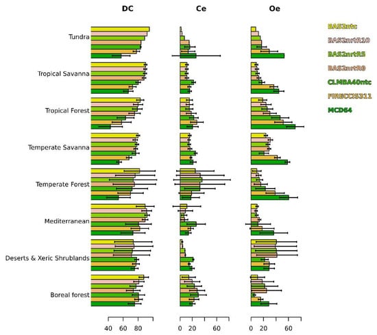
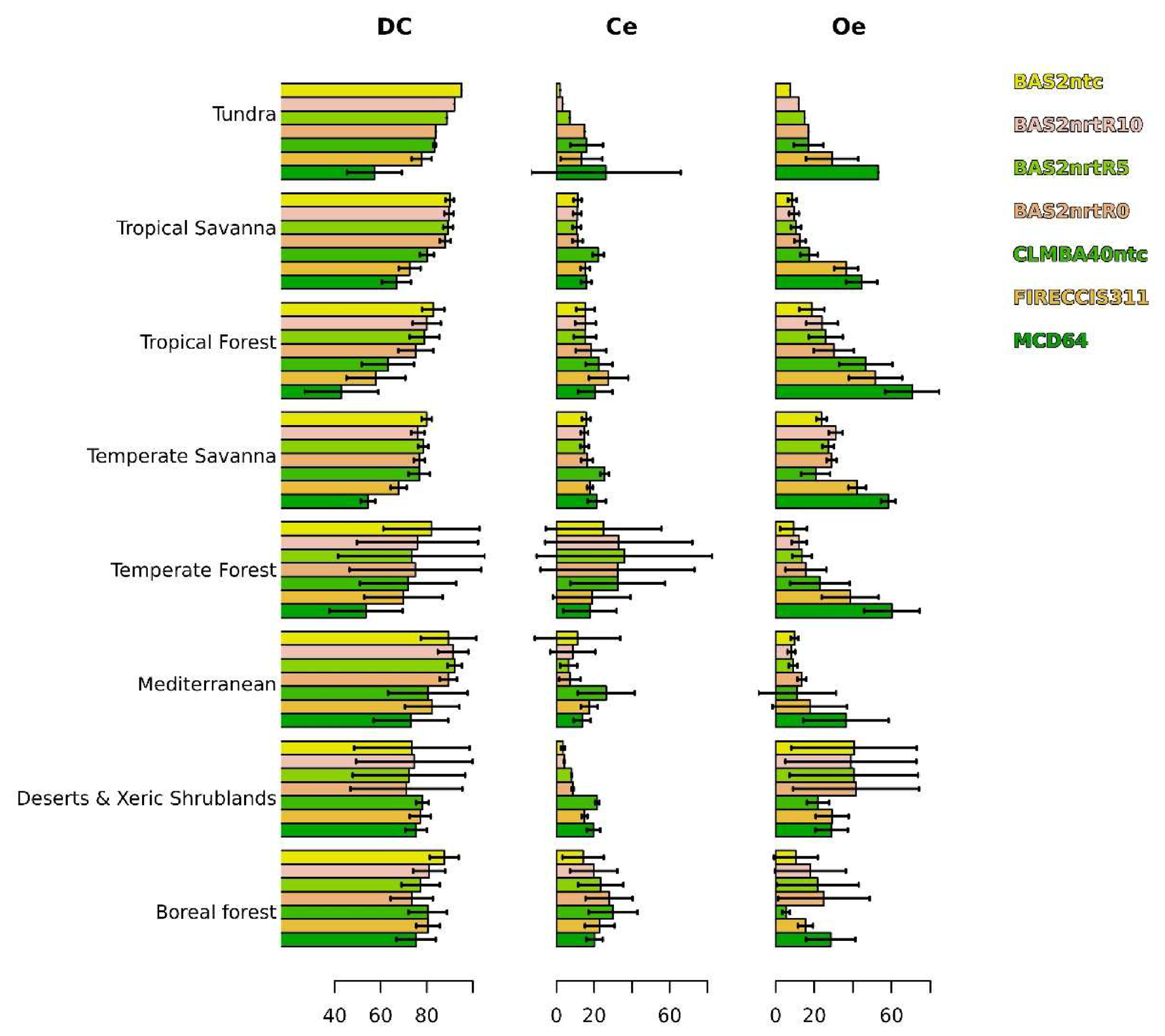
The accuracies inferred at global scale are somewhat replicated at biome level (Figure 10), particularly for two of the eight biomes: Tropical Savanna and Tropical Forest. Departures from global inferences vary across the other biomes, particularly in Boreal Forest, Deserts and Xeric Shrublands, where the accuracy of the Sentinel-2 BA mapping is similar to, and lower than, that of the coarse-resolution products. Particularly in the latter case, the uncertainty in the Sentinel-2 BA accuracy is remarkably large (see the large 95% confidence intervals in Figure 10).

Figure 10. Per-biome inferences of accuracy for 2019, Dice coefficient (DC), commission error ratio (Ce), and omission error ratio (Oe) expressed as %. Error bars represent 95% confidence intervals.

4. Discussions

This study used a burned area (BA) mapping method based on deep learning developed originally for Sentinel-3 OLCI&SLSTR data [14] but implemented here for Sentinel-2 MSI data.

The relatively high neural network (NN) training performance with Sentinel-2 data, which increases with the length of the time series, similarly to what was observed with Sentinel-3 data [14], reflects the consistency of the NN architecture in retrieving accurate estimates regardless of the source of reflectance data. Likewise, the distinct distributions of burned and unburned reference classifications across the two-dimensional space of NN-predicted ${\mathrm{p}\mathrm{r}\mathrm{o}\mathrm{b}(f}_{\mathrm{b}}>0.1)$ and active fire detection density ($\mathrm{A}\mathrm{F}\mathrm{d}\mathrm{e}\mathrm{n}\mathrm{s}\mathrm{i}\mathrm{t}\mathrm{y}$), broadly similar in Sentinel-2 and -3 data, reflect the usefulness of a single logistic model to incorporate active fire information, regardless of the source of reflectance data. The flat curves around the selected thresholds of $\mathrm{p}\mathrm{r}\mathrm{o}\mathrm{b}\left(\mathrm{b}\right)$ (Figure 9) reflect the relatively low sensitivity of the output’s accuracy to the threshold selection.

The implementation of the NN convolutional layers on the temporal and spectral dimensions of the data enabled the use of a computationally efficient, relatively small neural network (<300,000 parameters). The generation of each daily NRT and monthly NTC product takes, on average, 6.5 and 19 min, and up to 20 and 40 GB of memory, respectively, per 100 km × 100 km Sentinel-2 tile. This is in the same order of magnitude as the computational runtimes of another Sentinel-2 BA algorithm run in Google Earth Engine [59]. In our case, the computational requirements were measured in a 15-CPUs (Intel(R) Core(TM) i7-10700K CPU @ 3.80 GHz) computer, generating products over a multiyear period covering a fire-prone region (approximately 10⁵ km²) in the north east of Spain.

The benefits of adding convolutional layers on the spatial dimension are unclear in the literature. While Belenguer-Plomer et al. [60] found there was no such benefit, other studies successfully implemented convolutional layers simultaneously on the spatial, temporal and spectral dimensions [26,61,62], however, needing very large NNs and training data made of pre-existent global BA products to estimate BA at very coarse 0.01–0.25° spatial resolutions. The large size of such NNs, up to 3.5 million parameters [26], may lead to computationally expensive algorithms, which can be of concern for NRT applications. Furthermore, using global BA products as training data might lead to the transfer of product quality issues into NN predictions. Therefore, further research should be conducted to ensure the NNs’ computational efficiency and to generate large amounts of high-quality spatio-temporal training data.

The accuracy of the Sentinel-2 NTC BA, BAS2ntc, Dice coefficient (DC) 87.2%, is slightly higher than the accuracy of the equivalent Sentinel-2 BA algorithm available in the literature, developed by Bastarrika et al. [22] (DC 81.8%), also evaluated with the same 2019 C3S reference dataset but using the full spatial extent of the sampled units, 100 × 100 km²—commonly referred to as cluster size in the sampling design literature ([54], Chapter 9). The use of a smaller cluster size in this study (40 × 40 km²) did not increase the uncertainty of the accuracy estimates: the magnitudes of the standard errors of the accuracy estimates reported here (Table 2) are similar to those in Bastarrika et al. [22]. This might reflect a strong positive intracluster spatial autocorrelation of errors, similarly as in previous BA validation exercises [63]. Positive spatial autocorrelation is common in the spatial distribution of classification errors [53]. It might explain the limited extra information added when cluster sizes are increased, leading to limited reductions in the uncertainty of estimates.

Table 2. Global inferences of accuracy for 2019, Dice coefficient (DC), commission error ratio (Ce), omission error ratio (Oe) and relative bias (relB) expressed as %. Standard errors are shown in parentheses.

Product	DC (%)	relB (%)	Ce (%)	Oe (%)
BAS2ntc	87.2 (1.0)	0.7 (1.7)	13.2 (1.1)	12.5 (1.4)
BAS2nrtR10	85.4 (1.3)	−2.2 (2.2)	13.6 (1.3)	15.5 (1.9)
BAS2nrtR5	84.7 (1.4)	−3.5 (2.4)	13.7 (1.5)	16.7 (2.0)
BAS2nrtR0	82.7 (1.6)	−5.2 (2.8)	15.0 (1.7)	19.5 (2.2)
CLMBA40ntc	75.6 (1.8)	−3.4 (3.5)	23.0 (1.3)	25.7 (2.8)
FIRECCIS311	68.7 (2.4)	−26.4 (2.6)	19.0 (1.6)	40.4 (2.9)
MCD64	60.3 (3.1)	−42.6 (3.7)	17.2 (1.3)	52.5 (3.5)

The higher accuracy of BA as timeliness decreases (Table 2) reflects the expected benefits of using reflectance observations after the mapping period, which help reduce false BA detections caused by cloud shadows. The highest gains in accuracy at the shortest prediction latencies—DC increases 2% between 0 and 5 days of latency (between BAS2nrt0 and BAS2nrt5) and 0.7% between 5 and 10 days (between BAS2nrt5 and BAS2nrt10)—indicate the effects of the reflectance observations availability following the mapping periods, particularly when those are scarce.

The large uncertainties in the accuracy estimates for some products in some biomes and the relatively large variability in differences between products at the biome level reflect the small validation sample sizes allocated in some biomes. It is important to emphasise that the sample allocation in the C3S reference datasets was designed to provide accurate estimates at the global level, not at the biome level [30,54]. Therefore, per-biome accuracy results must be interpreted with caution. Small sample sizes together with large variability in accuracies in some biomes might raise questions about the validity of accuracy inferences in some cases [30,54].

The results of this study demonstrate that a semi-empirical and deep learning-based method, originally designed for Sentinel-3 OLCI&SLSTR data [14], can be used to retrieve highly accurate BA estimates from Sentinel-2 MSI data. The high accuracies of Sentinel-2 and -3 BA estimates, in both cases higher than equivalent global products, yet retrieved by a single BA mapping method, provide support for the sensor independence of this method, which can be critical for integrating ever-evolving satellite technologies and expanding fire-monitoring systems. Such sensor independence could be key to facilitating the transfer of developments from one satellite sensor to another and keeping the costs of monitoring system development down. Our work provides opportunities to develop new BA monitoring systems by combining existing missions’ data (e.g., Sentinel-2 and Landsat) or integrating new satellite instruments, such as the EUMETSAT geostationary MTG-FCI, which has been available since September 2024 and delivers 0.5–1 km radiance imagery every 10 min. In the latter case, some modifications are needed to ingest radiance instead of reflectance observations. Additionally, the mapping method used here is able to provide estimates at several levels of latency—with accuracy estimates increasing along with latency. BA estimates are retrieved as daily maps at NRT, with 0, 5, and 10 days of latency relative to the mapping day, and as monthly mosaics at NTC with 45 days of latency. Such capability might facilitate the usage of BA products in time-critical wildfire impact applications by providing a range of choices with several levels of accuracy and latency.

5. Conclusions

This study presents the results of the calibration and the validation of a burned area (BA) mapping method, based on semi-empirical modelling and deep learning, originally developed for Sentinel-3 OLCI&SLSTR data but implemented here with Sentinel-2 MSI data. The mapping method uses a neural network (NN) with two blocks of 1-dimensional convolutional layers applied to the temporal and spectral dimensions of the data, along with a bidirectional Long Short-Term Memory layer. Additionally, a logistic model is used to account for the spatio-temporal density of active fire detections. The similar NN training performance and logistic regression results obtained here with Sentinel-2 data, compared to those with Sentinel-3 data, indicate the usefulness of this mapping method regardless of the source of reflectance data. Additionally, the mapping method used here is able to provide BA estimates across a wide range of latencies. The accuracy of the estimates increases with the latency, which allows for a higher amount of observations posterior to the mapping period and helps avoid false positive classifications caused by cloud shadows. Similarly, and as is the case for Sentinel-3, Sentinel-2 BA estimates have a similar or higher accuracy—DC 82.7% for daily maps with 0 days of latency, DC 84.7% with 5 days, DC 85.4% with 10 days, and DC 87.2% for monthly composites derived on a non-time critical basis (NTC) with 45 days of latency—than equivalent global algorithms found in the literature, in this case only one—DC 81.8% for NTC BA.

References

- Cunningham, C.X.; Williamson, G.J.; Bowman, D.M. Increasing Frequency and Intensity of the Most Extreme Wildfires on Earth. Nat. Ecol. Evol. 2024, 8, 1420–1425. [Google Scholar] [CrossRef] [Scilit] [PubMed]
- Zantout, K.; Balkovic, J.; Billing, M.; Folberth, C.; Gosling, S.N.; Hank, T.; Hantson, S.; Iizumi, T.; Ito, A.; Jägermeyr, J.; et al. Shifting Dominant Periods in Extreme Climate Impacts under Global Warming. Nat. Commun. 2025, 16, 9746. [Google Scholar] [CrossRef] [Scilit]
- Bowman, D.; Kolden, C.A.; Abatzoglou, J.T.; Johnston, F.H.; van der Werf, G.R.; Flannigan, M. Vegetation Fires in the Anthropocene. Nat. Rev. Earth Environ. 2020, 1, 500–515. [Google Scholar] [CrossRef] [Scilit]
- Jolly, W.M.; Cochrane, M.A.; Freeborn, P.H.; Holden, Z.A.; Brown, T.J.; Williamson, G.J.; Bowman, D.M. Climate-Induced Variations in Global Wildfire Danger from 1979 to 2013. Nat. Commun. 2015, 6, 7537. [Google Scholar] [CrossRef] [Scilit]
- Bowman, D.; Williamson, G.; Yebra, M.; Lizundia-Loiola, J.; Pettinari, M.L.; Shah, S.; Bradstock, R.; Chuvieco, E. Wildfires: Australia Needs National Monitoring Agency. Nature 2020, 584, 188–191. [Google Scholar] [CrossRef] [Scilit]
- Mason, P.; Zillman, J.; Simmons, A.; Lindstrom, E.; Harrison, D.; Dolman, H.; Bojinski, S.; Fischer, A.; Latham, J.; Rasmussen, J.; et al. Implementation Plan for the Global Observing System for Climate in Support of the UNFCCC (2010 Update); World Meteorological Organization: Geneva, Switzerland, 2010. [Google Scholar]
- Chen, Y.; Hall, J.; Van Wees, D.; Andela, N.; Hantson, S.; Giglio, L.; Van Der Werf, G.R.; Morton, D.C.; Randerson, J.T. Multi-Decadal Trends and Variability in Burned Area from the 5th Version of the Global Fire Emissions Database (GFED5). Earth Syst. Sci. Data Discuss. 2023, 2023, 5227–5259. [Google Scholar] [CrossRef] [Scilit]
- Seiler, W.; Crutzen, P.J. Estimates of Gross and Net Fluxes of Carbon between the Biosphere and the Atmosphere from Biomass Burning. Clim. Change 1980, 2, 207–247. [Google Scholar] [CrossRef] [Scilit]
- van der Werf, G.R.; Randerson, J.T.; Giglio, L.; Collatz, G.J.; Kasibhatla, P.S.; Arellano, A.F., Jr. Interannual Variability in Global Biomass Burning Emissions from 1997 to 2004. Atmos. Chem. Phys. 2006, 6, 3423–3441. [Google Scholar] [CrossRef] [Scilit]
- Giglio, L.; Boschetti, L.; Roy, D.P.; Humber, M.L.; Justice, C.O. The Collection 6 MODIS Burned Area Mapping Algorithm and Product. Remote Sens. Environ. 2018, 217, 72–85. [Google Scholar] [CrossRef] [Scilit]
- Alonso-Canas, I.; Chuvieco, E. Global Burned Area Mapping from ENVISAT-MERIS and MODIS Active Fire Data. Remote Sens. Environ. 2015, 163, 140–152. [Google Scholar] [CrossRef] [Scilit]
- Chuvieco, E.; Lizundia-Loiola, J.; Lucrecia Pettinari, M.; Ramo, R.; Padilla, M.; Tansey, K.; Mouillot, F.; Laurent, P.; Storm, T.; Heil, A.; et al. Generation and Analysis of a New Global Burned Area Product Based on MODIS 250 m Reflectance Bands and Thermal Anomalies. Earth Syst. Sci. Data 2018, 10, 2015–2031. [Google Scholar] [CrossRef] [Scilit]
- Lizundia-Loiola, J.; Franquesa, M.; Khairoun, A.; Chuvieco, E. Global Burned Area Mapping from Sentinel-3 Synergy and VIIRS Active Fires. Remote Sens. Environ. 2022, 282, 113298. [Google Scholar] [CrossRef] [Scilit]
- Padilla, M.; Ramo, R.; Gomez-Dans, J.; Sierra, S.; Mota, B.; Lacaze, R.; Tansey, K. Near-Real Time Monitoring of Burned Area at Global Scale Based on Deep Learning. Int. J. Remote Sens. 2025, 46, 5996–6038. [Google Scholar] [CrossRef] [Scilit]
- Roteta, E.; Bastarrika, A.; Padilla, M.; Storm, T.; Chuvieco, E. Development of a Sentinel-2 Burned Area Algorithm: Generation of a Small Fire Database for Sub-Saharan Africa. Remote Sens. Environ. 2019, 222, 1–17. [Google Scholar] [CrossRef] [Scilit]
- Roy, D.P.; Huang, H.; Boschetti, L.; Giglio, L.; Yan, L.; Zhang, H.H.; Li, Z. Landsat-8 and Sentinel-2 Burned Area Mapping-A Combined Sensor Multi-Temporal Change Detection Approach. Remote Sens. Environ. 2019, 231, 111254. [Google Scholar] [CrossRef] [Scilit]
- Ramo, R.; Roteta, E.; Bistinas, I.; Van Wees, D.; Bastarrika, A.; Chuvieco, E.; Van der Werf, G.R. African Burned Area and Fire Carbon Emissions Are Strongly Impacted by Small Fires Undetected by Coarse Resolution Satellite Data. Proc. Natl. Acad. Sci. USA 2021, 118, e2011160118. [Google Scholar] [CrossRef] [Scilit] [PubMed]
- Oliveira, S.L.; Pereira, J.M.; Carreiras, J.M. Fire Frequency Analysis in Portugal (1975–2005), Using Landsat-Based Burnt Area Maps. Int. J. Wildland Fire 2012, 21, 48–60. [Google Scholar] [CrossRef] [Scilit]
- Goodwin, N.R.; Collett, L.J. Development of an Automated Method for Mapping Fire History Captured in Landsat TM and ETM+ Time Series across Queensland, Australia. Remote Sens. Environ. 2014, 148, 206–221. [Google Scholar] [CrossRef] [Scilit]
- Hardtke, L.A.; Blanco, P.D.; del Valle, H.F.; Metternicht, G.I.; Sione, W.F. Semi-Automated Mapping of Burned Areas in Semi-Arid Ecosystems Using MODIS Time-Series Imagery. Int. J. Appl. Earth Obs. Geoinf. 2015, 38, 25–35. [Google Scholar] [CrossRef] [Scilit]
- Hawbaker, T.J.; Vanderhoof, M.K.; Schmidt, G.L.; Beal, Y.-J.; Picotte, J.J.; Takacs, J.D.; Falgout, J.T.; Dwyer, J.L. The Landsat Burned Area Algorithm and Products for the Conterminous United States. Remote Sens. Environ. 2020, 244, 111801. [Google Scholar] [CrossRef] [Scilit]
- Bastarrika, A.; Rodriguez-Montellano, A.; Roteta, E.; Hantson, S.; Franquesa, M.; Torre, L.; Gonzalez-Ibarzabal, J.; Artano, K.; Martinez-Blanco, P.; Mesanza, A.; et al. An Automatic Procedure for Mapping Burned Areas Globally Using Sentinel-2 and VIIRS/MODIS Active Fires in Google Earth Engine. ISPRS J. Photogramm. Remote Sens. 2024, 218, 232–245. [Google Scholar] [CrossRef] [Scilit]
- Chuvieco, E.; Roteta, E.; Sali, M.; Stroppiana, D.; Boettcher, M.; Kirches, G.; Storm, T.; Khairoun, A.; Pettinari, M.L.; Franquesa, M.; et al. Building a Small Fire Database for Sub-Saharan Africa from Sentinel-2 High-Resolution Images. Sci. Total Environ. 2022, 845, 157139. [Google Scholar] [CrossRef] [Scilit]
- Long, T.; Zhang, Z.; He, G.; Jiao, W.; Tang, C.; Wu, B.; Zhang, X.; Wang, G.; Yin, R. 30 m Resolution Global Annual Burned Area Mapping Based on Landsat Images and Google Earth Engine. Remote Sens. 2019, 11, 489. [Google Scholar] [CrossRef] [Scilit]
- Roy, D.P.; Jin, Y.; Lewis, P.; Justice, C. Prototyping a Global Algorithm for Systematic Fire-Affected Area Mapping Using MODIS Time Series Data. Remote Sens. Environ. 2005, 97, 137–162. [Google Scholar] [CrossRef] [Scilit]
- Pinto, M.M.; Libonati, R.; Trigo, R.M.; Trigo, I.F.; DaCamara, C.C. A Deep Learning Approach for Mapping and Dating Burned Areas Using Temporal Sequences of Satellite Images. ISPRS J. Photogramm. Remote Sens. 2020, 160, 260–274. [Google Scholar] [CrossRef] [Scilit]
- Yuan, Y.; Lin, L.; Huo, L.-Z.; Kong, Y.-L.; Zhou, Z.-G.; Wu, B.; Jia, Y. Using an Attention-Based LSTM Encoder–Decoder Network for near Real-Time Disturbance Detection. IEEE J. Sel. Top. Appl. Earth Obs. Remote Sens. 2020, 13, 1819–1832. [Google Scholar] [CrossRef] [Scilit]
- Zhao, Y.; Ban, Y. Near Real-Time Wildfire Progression Mapping with VIIRS Time-Series and Autoregressive SwinUNETR. Int. J. Appl. Earth Obs. Geoinf. 2025, 136, 104358. [Google Scholar] [CrossRef] [Scilit]
- Nolde, M.; Rösch, M.; Riedlinger, T.; Taubenböck, H. Multi-Sensor near-Realtime Burnt Area Monitoring Using a Superpixel-Based Graph Convolutional Network Approach. GIScience Remote Sens. 2025, 62, 2498188. [Google Scholar] [CrossRef] [Scilit]
- Franquesa, M.; Lizundia-Loiola, J.; Stehman, S.V.; Chuvieco, E. Using Long Temporal Reference Units to Assess the Spatial Accuracy of Global Satellite-Derived Burned Area Products. Remote Sens. Environ. 2022, 269, 112823. [Google Scholar] [CrossRef] [Scilit]
- Lewis, P.; Quaife, T.; Gomez-Dans, J.; Disney, M.; Wooster, M.; Roy, D.; Pinty, B. Modelling the Impact of Wildfire on Spectral Reflectance. In Proceedings of the 2009 IEEE International Geoscience and Remote Sensing Symposium, Cape Town, South Africa, 12–17 July 2009; IEEE: New York, NY, USA, 2009; Volume 4, pp. IV-1019–IV-1022. [Google Scholar]
- Roy, D.P.; Landmann, T. Characterizing the Surface Heterogeneity of Fire Effects Using Multi-Temporal Reflective Wavelength Data. Int. J. Remote Sens. 2005, 26, 4197–4218. [Google Scholar] [CrossRef] [Scilit]
- LeCun, Y.; Boser, B.; Denker, J.; Henderson, D.; Howard, R.; Hubbard, W.; Jackel, L. Handwritten Digit Recognition with a Back-Propagation Network. Adv. Neural Inf. Process. Syst. 1989, 2, 396–404. [Google Scholar]
- Hochreiter, S.; Schmidhuber, J. Long Short-Term Memory. Neural Comput. 1997, 9, 1735–1780. [Google Scholar] [CrossRef] [Scilit]
- Li, X.; Strahler, A.H. Geometric-Optical Bidirectional Reflectance Modeling of the Discrete Crown Vegetation Canopy: Effect of Crown Shape and Mutual Shadowing. IEEE Trans. Geosci. Remote Sens. 1992, 30, 276–292. [Google Scholar]
- Ross, J. The Radiation Regime and Architecture of Plant Stands; Springer Science & Business Media: The Hague, The Netherlands, 1981. [Google Scholar]
- Louis, J. Sentinel-2 L2A Algorithm Theoretical Basis Document; ESA: Paris, France, 2021. [Google Scholar]
- Schroeder, W.; Giglio, L. NASA VIIRS Land Science Investigator Processing System (SIPS) Visible Infrared Imaging Radiometer Suite (VIIRS) 375 m & 750 m Active Fire Products: Product User’s Guide Version 1.4. Prod. User’s Guide Version 2018, 1, 23. [Google Scholar]
- LANCE. LANCE Near Real Time (NRT). Available online: https://nrt4.modaps.eosdis.nasa.gov/archive/FIRMS (accessed on 9 July 2022).
- FIRMS. Fire Information for Resource Management System. Available online: https://firms.modaps.eosdis.nasa.gov/map (accessed on 9 July 2022).
- Schroeder, W.; Oliva, P.; Giglio, L.; Csiszar, I.A. The New VIIRS 375 m Active Fire Detection Data Product: Algorithm Description and Initial Assessment. Remote Sens. Environ. 2014, 143, 85–96. [Google Scholar]
- Zhang, T.; Wooster, M.J.; Xu, W. Approaches for Synergistically Exploiting VIIRS I-and M-Band Data in Regional Active Fire Detection and FRP Assessment: A Demonstration with Respect to Agricultural Residue Burning in Eastern China. Remote Sens. Environ. 2017, 198, 407–424. [Google Scholar]
- C3S Land Cover Classification Gridded Maps from 1992 to Present Derived from Satellite Observation. Available online: https://cds.climate.copernicus.eu/datasets/satellite-land-cover?tab=overview (accessed on 17 January 2025).
- Trigg, S.; Flasse, S. An Evaluation of Different Bi-Spectral Spaces for Discriminating Burned Shrub-Savannah. Int. J. Remote Sens. 2001, 22, 2641–2647. [Google Scholar]
- Pereira, J.M.; Sá, A.C.; Sousa, A.M.; Silva, J.M.; Santos, T.N.; Carreiras, J.M. Spectral Characterisation and Discrimination of Burnt Areas. In Remote Sensing of Large Wildfires: In the European Mediterranean Basin; Springer: Berlin/Heidelberg, Germany, 1999; pp. 123–138. [Google Scholar]
- van Dijk, D.; Shoaie, S.; van Leeuwen, T.; Veraverbeke, S. Spectral Signature Analysis of False Positive Burned Area Detection from Agricultural Harvests Using Sentinel-2 Data. Int. J. Appl. Earth Obs. Geoinf. 2021, 97, 102296. [Google Scholar]
- De Fauw, J.; Ledsam, J.R.; Romera-Paredes, B.; Nikolov, S.; Tomasev, N.; Blackwell, S.; Askham, H.; Glorot, X.; O’Donoghue, B.; Visentin, D.; et al. Clinically Applicable Deep Learning for Diagnosis and Referral in Retinal Disease. Nat. Med. 2018, 24, 1342–1350. [Google Scholar] [CrossRef] [Scilit]
- Glorot, X.; Bengio, Y. Understanding the Difficulty of Training Deep Feedforward Neural Networks. In Proceedings of the Thirteenth International Conference on Artificial Intelligence and Statistics, Sardinia, Italy, 13–15 May 2010; JMLR Workshop and Conference Proceedings; JMLR: Norfolk, MA, USA, 2010; pp. 249–256. [Google Scholar]
- Abadi, M.; Barham, P.; Chen, J.; Chen, Z.; Davis, A.; Dean, J.; Devin, M.; Ghemawat, S.; Irving, G.; Isard, M.; et al. TensorFlow: A System for Large-Scale Machine Learning. In Proceedings of the 12th USENIX Symposium on Operating Systems Design and Implementation (OSDI 16), Savannah, GA, USA, 2–4 November 2016; USENIX Association: Berkeley, CA, USA, 2016; pp. 265–283. [Google Scholar]
- Kingma, D.P.; Ba, J. A Method for Stochastic Optimization. arXiv 2014, arXiv:1412.6980. [Google Scholar] [CrossRef] [Scilit]
- Franquesa, M.; Vanderhoof, M.K.; Stavrakoudis, D.; Gitas, I.Z.; Roteta, E.; Padilla, M.; Chuvieco, E. Development of a Standard Database of Reference Sites for Validating Global Burned Area Products. Earth Syst. Sci. Data 2020, 12, 3229–3246. [Google Scholar] [CrossRef] [Scilit]
- Dinerstein, E.; Olson, D.; Joshi, A.; Vynne, C.; Burgess, N.D.; Wikramanayake, E.; Hahn, N.; Palminteri, S.; Hedao, P.; Noss, R.; et al. An Ecoregion-Based Approach to Protecting Half the Terrestrial Realm. BioScience 2017, 67, 534–545. [Google Scholar] [CrossRef] [Scilit]
- Stehman, S.V. Estimating Standard Errors of Accuracy Assessment Statistics under Cluster Sampling. Remote Sens. Environ. 1997, 60, 258–269. [Google Scholar]
- Padilla, M.; Olofsson, P.; Stehman, S.V.; Tansey, K.; Chuvieco, E. Stratification and Sample Allocation for Reference Burned Area Data. Remote Sens. Environ. 2017, 203, 240–255. [Google Scholar]
- Cochran, W.G. Sampling Methods, 3rd ed.; John Wiley & Sons: New York, NY, USA, 1977. [Google Scholar]
- Padilla, M.; Stehman, S.V.; Ramo, R.; Corti, D.; Hantson, S.; Oliva, P.; Alonso-Canas, I.; Bradley, A.V.; Tansey, K.; Mota, B.; et al. Comparing the Accuracies of Remote Sensing Global Burned Area Products Using Stratified Random Sampling and Estimation. Remote Sens. Environ. 2015, 160, 114–121. [Google Scholar]
- Dice, L.R. Measures of the Amount of Ecologic Association between Species. Ecology 1945, 26, 297–302. [Google Scholar] [CrossRef] [Scilit]
- Bradley, A.P. The Use of the Area under the ROC Curve in the Evaluation of Machine Learning Algorithms. Pattern Recognit. 1997, 30, 1145–1159. [Google Scholar] [CrossRef] [Scilit]
- Roteta, E.; Bastarrika, A.; Franquesa, M.; Chuvieco, E. Landsat and Sentinel-2 Based Burned Area Mapping Tools in Google Earth Engine. Remote Sens. 2021, 13, 816. [Google Scholar]
- Belenguer-Plomer, M.A.; Tanase, M.A.; Chuvieco, E.; Bovolo, F. CNN-Based Burned Area Mapping Using Radar and Optical Data. Remote Sens. Environ. 2021, 260, 112468. [Google Scholar] [CrossRef] [Scilit]
- Masolele, R.N.; De Sy, V.; Herold, M.; Marcos, D.; Verbesselt, J.; Gieseke, F.; Mullissa, A.G.; Martius, C. Spatial and Temporal Deep Learning Methods for Deriving Land-Use Following Deforestation: A Pan-Tropical Case Study Using Landsat Time Series. Remote Sens. Environ. 2021, 264, 112600. [Google Scholar]
- Zhang, G.; Wang, M.; Liu, K. Dynamic Prediction of Global Monthly Burned Area with Hybrid Deep Neural Networks. Ecol. Appl. 2022, 32, e2610. [Google Scholar] [CrossRef] [Scilit] [PubMed]
- Padilla, M.; Stehman, S.V.; Chuvieco, E. Validation of the 2008 MODIS-MCD45 Global Burned Area Product Using Stratified Random Sampling. Remote Sens. Environ. 2014, 144, 187–196. [Google Scholar] [CrossRef] [Scilit]
Disclaimer/Publisher’s Note: The statements, opinions and data contained in all publications are solely those of the individual author(s) and contributor(s) and not of MDPI and/or the editor(s). MDPI and/or the editor(s) disclaim responsibility for any injury to people or property resulting from any ideas, methods, instructions or products referred to in the content. |
© 2026 by the authors. Licensee MDPI, Basel, Switzerland. This article is an open access article distributed under the terms and conditions of the Creative Commons Attribution (CC BY) license.