


Abstract
Bioaerosols released during wildland and prescribed fires may influence ecosystems, air quality, and microbial dispersal, yet their transport and deposition remain poorly understood. This study combined infrared uncrewed aircraft system (UAS) observations of a prescribed burn with the coupled fire–atmosphere model WRF-SFIRE and a Lagrangian particle model in order to evaluate how uncertainties in simulated fire behavior affect predicted bioaerosol (bacterial cell) transport and deposition. A reconstruction of the observed spatiotemporal evolution of the fire was derived from thermal UAS measurements acquired during the burn and incorporated into a WRF-SFIRE simulation, in which the modeled fire spread was constrained to follow this reconstructed progression. This benchmark run was compared with two unconstrained, fully coupled simulations that used a low and a high estimate of fuel moisture content (FMC) to represent typical uncertainty in fire rate of spread (ROS) prediction. Despite substantial differences in fire intensity and plume dynamics among the simulations, the resulting bioaerosol transport pathways and deposition patterns were broadly consistent across cases. The horizontal transport of the bioaerosols was dominated by the ambient Easterly wind and the bioaerosols were lofted by fire-affected updrafts—some exceeding 10 m/s—within the buoyant plume structure resolved in WRF-SFIRE. Deposition hot-spots appeared in consistent locations in the three simulations, especially regions where topography forced up-slope transport. Although the most intense fire produced slightly greater local deposition—likely due to a combination of stronger fire-induced downdrafts and overturning from penetration into strong vertical wind shear above the boundary layer—differences were small relative to the overall deposition footprint. These results suggested that, for burns of this scale, bioaerosol transport and deposition predictions are relatively robust to realistic uncertainties in fire-behavior modeling. This finding indicates that coupled fire–atmosphere and particle-transport modeling frameworks could be employed to quantitatively forecast microbial transport and deposition during future controlled burn experiments.
1. Introduction
Living microorganisms, including bacteria and fungi, have been found to be aerosolized in the smoke emitted by biomass burning [1,2,3,4,5,6,7,8]. The composition and concentration of these bioaerosols within the microbiome of plumes of wildland fires have been shown to differ significantly from those of ambient conditions, with higher concentrations and diversity indicated across locations [4,8]. The strong updrafts observed in the pyro-convective plumes of wildland fires (up to 60 m/s) [9,10] have the potential to loft these bioaerosols into the atmosphere, where they may be transported and eventually deposited non-locally [6,7]. The transport and deposition of these plume-injected bioaerosols are of significant interest due to their potential effects on the ecology of the communities where the microorganisms are deposited, their atmospheric role as ice-nucleating particles, as well as their potential significance as drivers of ecosystem connections [3,7,8]. Despite their potential influence and importance, observational investigation of the transport and deposition of fire-aerosolized microorganisms remains challenging, particularly due to inherent difficulties in collecting observations of these bioaerosols both aloft and after deposition near active fires.
However, advances in technology have enabled the deployment of uncrewed aircraft systems (UAS) in an attempt to overcome these difficulties: UAS have been used to observe wildland fire behavior and estimate metrics like fire rate of spread, fuel consumption, and fire progression from thermal and near-infrared imagery [11,12,13,14,15], and UAS-mounted bioaerosol sampling was recently used to collect, profile, and quantify bioaerosol samples directly over wildland fires [1,7]. In one such case, UAS were employed during the Fire and Smoke Model Evaluation Experiment (FASMEE) burns near Richfield, UT, USA [16,17]. During this experimental burn, UAS collected measurements of the concentration and composition of lofted bioaerosols [1,4]. These observations provided novel insights into microbial smoke composition and enabled the estimation of bioaerosol emission factors [2], but these observations alone were not sufficient to fully characterize the transport of bioaerosols emitted during the burn, and their deposition was not observed. Further analysis of the emission, transport, and deposition of bioaerosols emitted from wildland fires could be critical for bettering current assessments of their ecological impacts on larger scales. So, alongside direct (but spatially sparse) observation of fire-borne bioaerosols both aloft and deposited, the capability to simulate their release, transport, and deposition is essential for assessing the potential reach of these ecological impacts. It is also crucial for improving experimental and prescribed burn planning, where more data could be collected, particularly when combined with spatially explicit fire behavior measurements [12,15].
In prior work, to address this need for a modeling framework capable of estimating the emission, transport, and deposition of fire-borne bioaerosols, a novel bioaerosol modeling framework was established and used to make a spatially explicit estimation of the emission, transport, and deposition of bioaerosols emitted by one of the FASMEE experimental fires [2]. This framework combined the fire progression and fire-influenced wind fields from the WRF-SFIRE [18,19] coupled fire–atmosphere forecast of the FASMEE burn with a Lagrangian particle transport model that resolved the deposition of bioaerosols released during the fire [2]. In this framework, WRF-SFIRE resolved the fire-driven plume dynamics and fire progression that were used to drive the particle transport model to render the transport of these bioaerosols. WRF-SFIRE has demonstrated the ability to render plume top heights from wildland fires with accuracies within hundreds of meters of observations [20,21], which made it a strong candidate to use to simulate the near-fire circulation, fire-induced plume, and larger-scale winds controlling the transport of fire-borne bioaerosols.
While this WRF-SFIRE-based modeling framework was the first and only effort known to the authors towards modeling the transport and deposition of fire-borne bioaerosols [2], other particle transport frameworks exist [22,23,24]. Despite the capability of these frameworks to couple the resolved background flow from coupled fire–atmosphere models with particle transport solvers, they are designed to model the flight trajectories and landings of particles (mostly firebrands) with characteristic length scales of 0.01 m, which is orders of magnitude larger than the characteristic length of aerosolized bacteria, that is, 1 μm. In effect, the governing equations apply to particles with low Stokes numbers, . In this regime, the Brownian motion due to turbulence and the thermal interactions of aerosolized particles with the air become important, whereas they are ignored in other regimes. Hence, the aforementioned frameworks are not suitable for simulating fire-borne bioaerosol transport. Therefore, in this study, the framework presented in [2] is employed to simulate the transport and fate of fire-borne bioaerosols on large spatiotemporal scales.
The estimation of a fire’s progression in WRF-SFIRE relies on the rate of spread model (in this case [25]), which has been shown to be highly dependent on factors including fuel moisture, classification, and characteristics [26,27]. Capturing the spatial variability of these factors with observations on the scale of WRF-SFIRE’s grid is challenging, and a truncated representation of the spatial patterns of these input parameters thus introduces a source of uncertainty into the fire simulations. These errors have the potential to propagate into the modeled fire intensity, smoke emissions, and the plume rise, raising the uncertainty in simulated microbial transport and deposition [28].
To reduce the uncertainties associated with the fire spread estimation, WRF-SFIRE can be executed with fire growth constrained by reconstructing fire progression based on observations—typically from satellite fire detections and infrared perimeters [21,29,30]. Such constrained fire progressions have utility in the modeling of wildfire events that are intense and large enough to be detected and resolved by satellite and infrared airborne observations. However, the applicability of this methodology is limited for the modeling of smaller, less intense fires that cannot be resolved in satellite products due to limitations in their temporal and spatial resolution [31]. This presents a challenge when using modeling to investigate bioaerosol transport and deposition during smaller prescribed fire experiments. Fortunately, the UAS deployed during some experimental burns can collect critical observations of fire spread. One such prescribed burn, where the necessary data in this study was collected, took place in a tallgrass prairie near Manhattan, Kansas, and provided an opportunity to overcome this challenge. The emission, transport, and deposition of bioaerosols via wildland fire have been explored in limited previous studies, with field-scale transport and deposition examined in [2] and laboratory characterization of emission processes from multiple fuel types recently conducted [32]. Motivated by the need to further advance bioaerosol modeling capabilities, this study leverages bioaerosol emission insights from both prescribed burns [2] and laboratory studies [32] along with UAS fire observations to simulate the transport and deposition of bioaerosols generated during a prescribed grass burn, and to evaluate the sensitivity of microbial transport and deposition to the representation of fire progression in WRF-SFIRE.
To do that, first, the observations collected by UAS during this burn were processed and used to produce a rasterized reconstruction of the progression of the fire. The UAS-based fire arrival time raster was then used to constrain fire progression in WRF-SFIRE simulations in order to render the evolution of the fire and the induced pyro-convective plume. These simulations were then used to drive simulations of the emission, transport, and deposition of bioaerosols emitted during the prescribed burn. Comparisons of simulations across different fuel moisture values present a novel test for the role of fuel characteristics on fire-driven bioaerosol dynamics, with relevance to future research on the role of prescribed fires in biological dispersal and biodiversity [6,7].
2. Methods
2.1. Experimental Burn Data
The prescribed burn of unit K1A of Kansas’ Konza tall grass prairie was conducted in April of 2022 as a part of the NSF-sponsored Biosmoke-Connect project and in concert with long-term prairie conservation-focused research on the seasonality and frequency of prescribed burning at the Konza Prairie Biological Station 10 km south of Manhattan, KS, USA (KPBS; 39°05′ N, 96°35′ W). The unit has been burned annually in the early spring season since at least 2005. This burn provided a unique dataset which characterized fuel properties, set ignition procedures, and collected infrared observations of the head fire’s progression [33].
The watershed’s grass-dominated fuels were classified into fuel categories with their assigned fuel properties presented in Table 1. The fuel map, based on K-means clustering of imagery of the burn plot from the National Agriculture Imagery Program (NAIP) was produced at 1 m resolution [34,35,36]. Each of the resulting categories was associated with the most representative fuel classes of the 40 Scott and Burgan fuel models [37], and assigned the respective fuel properties of their associated fuel model.
Table 1.
Fuel classification.
Three fuel moisture samples, 10.7%, 16.0%, and 23.0%, were collected using standard methods [38] in the morning before the burn’s ignition within three randomly located clip plots. It has to be noted that right before the burn, the fuel moisture could have been drier due to higher temperatures and lower relative humidity later in the day. These fuel moisture values could also have been influenced by the inclusion of some shrubs in the randomly distributed clip plots, which were primarily collected for biological assessments. However, other work has shown high variability in fuel moisture content across the KPBS even when characterizing exclusively grass samples [39], so it is hard to assess to what degree the inclusion of shrubs contributed to the variability across the samples. The burn plot’s most-representative fuel models (GR1, GR2, GR4, GR7) had a fuel moisture of extinction of 15%. So the higher fuel moisture content (FMC) measurement values, when used as input, would not allow the modeled fire to spread. This would not be consistent with actual fire behavior: readily spreading through the grass-dominated fuels within the burn plot. Therefore, 10.7%, the only value below the models’ fuel moisture of extinction, was chosen as the baseline fuel moisture content for the burn plot’s fuels in the simulations.
Additionally, near-surface winds were measured by a nearby National Ecological Observatory Network (NEON) tower. These observations were utilized to confirm that the simulations reasonably resolved the overall flow near the fire [40]. A primarily easterly/north-easterly wind prevailed for the duration of the burn, forcing a head fire that was ignited by drip torches along the eastern boundary of the plot. The head fire ignition team was equipped with a global positioning system (GPS) as they ignited the eastern plot boundary, starting from the northeast corner of the plot and walking south. Once the head fire ignition team reached the southeast corner of the plot, they continued west around the rest of the plot boundary, igniting a back fire. Leaving the northeast boundary at the same time as the primary ignition team, a second ignition team walked the northern plot boundary, igniting a second back fire. The head fire ignition team’s location data had to be used to estimate the speed at which the second team walked, under the assumption that both teams walked the boundary at a comparable speed, as this second ignition team was not equipped with a GPS. The fire spread was almost entirely from the head fire, traveling from the eastern boundary for the duration of the collection of UAS infrared observations; however, the backburn carried fire from the north and south later into the burn, with the fire area ultimately encompassing the entire burn plot—about 300 acres in size.
Most uniquely, high-resolution thermal infrared imagery of the advancing head fire was captured using a DJI Mavic 2 Enterprise Advanced UAS platform (SZ DJI Technology Co., Ltd., Shenzhen, China) The UAS was equipped with a 640 × 512 sensor with an 8–14 μm spectral resolution. This imagery of the progressing fire front was captured across seven UAS flight paths. These thermal images were then georeferenced and aligned into seven orthomosaics at a 0.25 m × 0.25 m resolution.
2.2. Fire Progression Reconstruction from Infrared Observations
The UAS thermal imagery was processed to reconstruct the fire progression and generate a spatially continuous representation of the temporal evolution of the fire’s position—a fire arrival time raster where each cell’s value represents the first time at which the fire arrived at that cell centroid [12,13]. To accomplish this, fire perimeters were heads-up digitized; perimeters separating the unburnt and burnt/burning area of the plot were digitized by tracing the approximate fire boundary using a view-dependent histogram normalization of the orthomosaics of the imagery from each flight. This allowed for an estimation of the fire perimeter’s location in areas where it would otherwise be difficult to discern due to lower local intensity in the infrared imagery. This methodology produced five complete fire perimeters, but two flights’ imagery covered too small a region of the fire to estimate a complete fire perimeter.
Unlike satellite data or airborne infrared perimeters [11,41], where an entire fire’s area is imaged almost instantaneously, these perimeters represent the fire’s location at the time at which the UAS imaged that section of the perimeter. During each flight, as the UAS flew over the fire front, small sections of the fire were imaged one at a time. As a result, each perimeter represents the fire front’s position at piecewise continuous time intervals along the perimeter derived from each flight. These perimeters are also spatiotemporally sparse, as the head fire advanced considerably between flights, leaving gaps between subsequent perimeters, along with gaps caused by incomplete imagery during the two flights.
To address these complexities, interpolation was performed at multiple stages. First, each perimeter was discretized into points spaced every 10 m along the fire perimeter. Second, these points were assigned the detection time of the nearest pixel in the infrared imagery. Third, lines were cast from front to front, connecting all combinations of pairs of these points between points on front i with points on front , similar to fire spread vector approaches used in prior work [11,14]. These pairs determined potential lines along which the fire may have spread from a point on front i to front . Fourth, these potential spread lines were then filtered based on several criteria: (i) Only spread lines completely contained within the growth area (the region contained in perimeter but not in perimeter i) were considered. (ii) From each source point, spread lines were retained if they were among the shortest 10% generated from that point. (iii) Lastly, the spread lines were filtered based on a normal angle metric, defined as the sum of the absolute differences between each line’s angle and the normal of the perimeter at both the originating and terminating points. For each originating point, 50% of the lines with the lowest values of this metric were retained. This filtering using criteria (i–iii) thus preserved spread lines that connected the nearest locations on the next observed fire perimeter where the perimeters were most similarly oriented. Fifth, the fire’s arrival time was interpolated at points every 10 m along each spread line from the known arrival time at each spread line’s endpoints on each front. This produced estimations of fire arrival time between the sparse fire perimeters from the UAS imagery.
Lastly, the fire arrival time data from the points between fronts and the arrival time data from the start and end points along the perimeters were collected and spatially interpolated to produce a rasterized fire arrival time for the region of the burn plot covered by the extent of the imagery. This spatial interpolation was completed using both Inverse Distance Weighted (IDW) and Natural Neighbors interpolation, two standard methods for interpolating point data spatially. In order to demonstrate the beneficial effects of the inclusion of points interpolated along the spread lines, both methods were also applied to the point data from the endpoints along the perimeters without the spread line data. The resulting four reconstruction rasters (IDW with and without the addition of the interpolated spread line data, and Natural Neighbors with and without the addition of the interpolated data), were then evaluated based on the independent fire arrival time observations from the two UAS flights that did not collect sufficient imagery of the entire front to estimate complete fire perimeters and thus were excluded for the fire arrival time reconstruction.
2.3. Modeling Framework
This study used a modeling framework consisting of the fire model (WRF-SFIRE version W4.4-S0.1) and a Lagrangian particle transport model. WRF-SFIRE provides information on fire heat fluxes and the resulting three-dimensional wind field, while the particle model uses these outputs to release particles and simulate their trajectories based on the WRF-SFIRE wind fields. Details of the two models are provided in the subsequent subsections.
2.3.1. Fire Model
The coupled fire–atmosphere model, WRF-SFIRE, was used to recreate the fire progression, fire behavior, plume rise, and smoke dispersion, including the 3D atmospheric flow in the pyroconvective column. The model was run, in all simulations, using the same nested grid configuration with 5 two-way nested domains with the grid spacing ranging from 1620 m to 20 m as shown in Table 2. The fire mesh in the innermost domain d05 was refined with a factor of 20, resulting in a fire mesh with a resolution of 1 m.
Table 2.
WRF-SFIRE model configuration options.
Simulations were completed using the fire model in two different configurations: free-run and constrained. The free-running simulations allowed the fire to spread from the walking ignition, according to the rate and direction of spread calculated by the model based on the fuel characteristics, topography, and wind conditions, computed within the fifth domain. The constrained simulation was completed with the fire’s spread controlled by a rasterized arrival time reconstruction. In this configuration, the model advances the fire at the speed and direction encoded in the observed fire arrival time. The results from the constrained run represent a replay of the fire’s progression based on the infrared observations, whereas the free-running simulations are more typical of a situation where only ignition information is known. An additional no-fire simulation was performed as well, to enable direct quantification of the fire-induced perturbations. This simulation produced a wind flow impacted by the topography of the domain without the impacts of the fire. This enabled the estimation of the fire-induced circulation for each of the coupled fire–atmosphere simulations by subtracting the wind field produced by the simulation with and without fire heat fluxes, cell by cell.
The head fire in the free-running simulations was ignited according to a walking ignition pattern along the eastern boundary of the plot, as determined by GPS data of the head fire ignition team’s location. However, because the infrared imagery allowed only the reconstruction of the first 53.75 min of the fire’s position, the constrained simulation was configured to replay the fire progression only until that moment. Afterwards, the model switched to the free-running mode and continued advancing the fire from its final observed perimeter according to local topography as well as fuel and weather conditions.
Additionally, at the end of the collected infrared observations, 53.75 min into the simulation, fuel was ignited and freely allowed to spread from the northern and southern boundaries of the plot in both free-running and constrained simulations to account for the back-burning. This procedure allowed both simulations (constrained and free) to follow the same ignition pattern so that the simulations were more directly comparable.
One of the free runs (labeled free run low-FMC) was completed with a constant fuel moisture content of 10.7%, the lowest of the fuel moisture contents observed on the day of the fire. In addition, to investigate the uncertainty associated with the two other fuel moisture content measurements that had to be disregarded, an additional free-running simulation (labeled free run high-FMC) was completed with an elevated constant fuel moisture content of 13.8%. This value was calculated as the baseline of 10.7% plus half the standard deviation computed from all three fuel moisture measurements (6.2%).
For all simulations, the scale-aware Large Eddy Simulation scheme, km_opt = 5, was selected for all atmospheric domains to accommodate grid resolutions within the PBL gray zone [42]. To better capture the fire-induced buoyancy and the resulting formation of pyroconvective plumes, the first vertical model layer was set at 10 m above ground. To allow for this change, the vertical grid was adjusted using auto_lvls option two, which gives model users more control over the spacing of the model’s vertical grid.
To determine the spatial extent of the smoke plume and to compute plume properties such as the vertical velocities within the plume core, a passive tracer field in WRF-SFIRE representing concentrations of particulate matter with diameter ≤ 2.5 μm (PM2.5) was used. Although this passive tracer is a simplified representation of particulate transport, it provides a practical diagnostic tool for analyzing WRF-SFIRE output. By applying a threshold value to the tracer concentration, we delineated the plume region and isolated grid cells influenced by the fire. In this study, we defined plume-affected cells as those with PM2.5 concentrations , using as a threshold for distinguishing areas inside versus outside the plume at each model time step.
2.3.2. Particle Transport Model
The dynamics of bioaerosols in wildfire plumes involve several transport mechanisms, including advection and turbulent diffusion driven by particle inertia and Brownian diffusion resulting from interactions with air molecules [43]. This work employs a highly scalable and adaptive Lagrangian numerical framework, developed to describe the transport and deposition of the aerosolized particles emitted through the interactions between combusting wildland fuels and the boundary layer [4]. Following [2], the model accounts for the drag force that adaptively changes between corrected Stokes’ law and empirical drag [44]. Also, the gravitational deposition is considered while the particles are assumed to be spherical and non-aqueous, that is, the shape effects and intra-particle forces with their cascading effects, such as coagulation and nucleation, are not considered. Additionally, the Basset history force is not considered.The resulting model leads to a stochastic differential equation similar to Langevin Dynamics, representing the dispersion of aerosols in turbulent flows [45,46]. The primary assumption in resolving the trajectories and deposition zones is to consider the stochastic dispersion as a Markovian Process [47,48]. Therefore, the model resolves the mean trajectories following the method of [45] and integrates the remaining terms using the technique presented in [48].
The physical properties of the particles, such as diameter, were defined based on results from the field and microscopy measurements [2,4]. The particle diameter was sampled from a uniform distribution ranging from 1 μm to 50 μm. Therefore, ninety percent of the particle diameters were randomly chosen from the uniform distribution μm and the remaining 10% were sampled from μm to align the distribution of bioaerosols (bacterial cells) observed through microscopy in smoke samples collected during the FASMEE burn [1,2,4], though recent studies show size distributions can vary with combustion conditions [32]. The density of the particles was considered to follow the measurements presented in [49] and was sampled from a uniform random distribution of kg/m3. For each timestamp of the fire progression, the particles were initialized uniformly throughout the active fire areas, where the modeled heat flux (GRNHFX variable in WRF-SFIRE) was greater than 5 kW/m2. Approximately five million particles were initialized per 5 min timestamp of the WRF-SFIRE to represent the spatial ensemble of the trajectories and deposition in a 11.58 × 11.58 km domain centered on the burn. The trajectories were computed based on the U, V, W wind speed components from the WRF-SFIRE domain d04. The particles’ positions were reported every minute until they were transported out of the domain or deposited. The number of particles was selected arbitrarily, and further work is needed to establish the statistical significance of the number of released particles throughout the landscape, as well as the relationships between bioaerosol flux, fuel consumption rate, and species yields. Recent laboratory characterizations of combustion-dependent emissions [32] provide insights for future parameterizations, though integrating these into the frameworks remains beyond this study’s scope. An example of a 3D rendering of the bioaerosol transport resolved by this modeling framework is presented in Figure 1.
Figure 1.
A 3D render (created using VAPOR v3.9.3 [50,51]) of the time-aggregated density(number particles per grid-cell volume) of emitted bioaerosols (shorthanded to BioD in this figure) in the particle simulation forced by the WRF-SFIRE run with the fire’s progression constrained to infrared observations. A time-averaged vertical wind profile is shown upwind of the burn plot in dark brown. Orographic height (HGT) above mean sea level is also shown.
3. Results and Discussion
3.1. Fire Progression Reconstruction
Infrared UAS observations of a prescribed burn in the Konza tall grass prairie provided a unique opportunity to investigate the effect of errors in fire behavior representation within WRF-SFIRE on the simulated transport and deposition of bioaerosols emitted during the burn. Since uncertainties in FMC have the potential to significantly change the modeled fire behavior and pyroconvection, the accuracy of the FMC representation used in the model could be critical when attempting to predict the transport paths and deposition locations of fire-borne bioaerosols. These considerations are important because measuring bioaerosol deposition at specific locations is difficult and costly, and observing its spatial patterns is even more challenging. The locations and concentrations are of broad relevance. For example, significant smoke-driven bioaerosol deposition in marine systems has been observed [52], and pathogenic bioaerosols have the potential to affect downwind population centers [3]. Studies have already indicated that different fuels and fire behavior produce different bioaerosol concentrations and composition in smoke [2,8,53]. For the bioaerosol modeling framework proposed in this study to be useful for planning and executing observations of bioaerosol deposition during prescribed-fire experiments, it must therefore be reasonably robust with respect to uncertainties in FMC data and to errors in the fire behavior simulated by WRF-SFIRE. To assess the robustness of the framework, a baseline representation of the observed fire progression had to be established. To do this, the sparse and discontinuous UAS thermal imagery of the head fire was processed into the continuous rasterized fire arrival maps presented in Figure 2, one of which was selected and used to constrain the fire spread within WRF-SFIRE.
Figure 2.
Estimations of the fire’s arrival time produced using the uncrewed aircraft system (UAS) thermal imagery reconstruction methodology. Plots (a–d) show the rasters produced when two different spatial interpolation methods were used on the data including and not including the spread lines between detected fronts: (a) Inverse Distance Weighted (IDW) interpolation applied to data only from the points along the 5 detected continuous fire perimeters, (b) Natural Neighbors interpolation applied to data only from the points along the 5 detected continuous fire perimeters, (c) IDW applied to points from along the perimeters in addition to points interpolated along front to front spread lines, (d) Natural Neighbors applied to points from along the perimeters in addition to points interpolated along front to front spread lines. One-minute contours are shown in black in (a–d).
These fire arrival time rasters were produced from two distinct sets of fire–arrival point features: one containing only points located directly along each observed fire front, and a second, more comprehensive set that included these points together with additional interpolated points generated using the spread-line interpolation method described above in Section 2.2. Each dataset was spatially interpolated twice—once using Inverse Distance Weighting (IDW) and once using Natural Neighbors—yielding four candidate fire progressions. The resulting reconstructions, shown in Figure 2, were compared to evaluate both their qualitative structure and quantitative agreement with the UAS observations.
As presented in the reconstructions in Figure 2a,b, the reconstructions interpolated from the data without the points generated between the perimeters along front-to-front spread lines resulted in large regions of quick fire spread between each of the perimeters and slower spread near these perimeters. This led to these reconstructions representing a fire progression where the area between each perimeter is ignited nearly all at once. This phenomenon is most clearly seen in Figure 2a. This unrealistic, stepwise progression of fire in grassy fuels, resulting in a very thick fire front, is not consistent with observations of fire front depth in tall grasses in physical models and experimental prescribed burning, which are typically on the scale of tens of meters or less [54,55]. Therefore, the rasterized fire progressions in Figure 2a,b that represent the fire as traveling large distances were excluded as not suitable for constraining the fire progression in the control simulation.
When examining the qualitative features of reconstructions interpolated with the addition of data from the linearly interpolated front-to-front spread lines, Figure 2c,d, it can be seen that these reconstructions are smooth and free from the aforementioned issue. The comparison between the progressions in Figure 2c,d indicates that the progression interpolated with IDW (c) is significantly smoother and less prone to interpolation artifacts than the progression using Natural Neighbors (d). Additionally, the reconstruction using IDW and the front-to-front interpolation presented in Figure 2c, despite representing the fire front’s progression most smoothly, retained a detailed representation of fine-scale fire behavior, such as the fire front fingering that could be seen approximately 35 min into the progression. At one location towards the southernmost edge of the fire front, the spread was slowed by the presence of shrubby woody fuels. This reconstruction maintained smooth fire progression in this region and correctly captured the fingering to the south of these woody fuels, after which, about 40 min into the progression, the finger was incorporated into the head of the fire. The other three reconstructions struggled to maintain any consistency in the fire front representation of this fine-scale fire behavior and produced non-physical artifacts unrepresentative of the observed fire behavior, especially exacerbated by the spatial complexity of the fingering/pocketing behavior in this region.
The data from the two incomplete UAS flights (1 and 5) were used to digitize partial perimeters that were then discretized into points every 10 m along the incomplete perimeters. The observed time of the fire’s arrival to the perimeter at each of these points was then compared to the rasterized value of the fire’s time of arrival at each of these points’ locations according to the predictions from each of the four rasters. This was done to assess how well each of the rasters estimated the time of arrival of the fire at points with known arrival times lying between the perimeters used to create the rasters; essentially, testing how well each of the four reconstruction methods performed.
For both IDW and Natural Neighbors interpolation, the addition of the spread line data improved the average error, as seen in Table 3. A small, but consistent negative bias in interpolated fire arrival was observed. The reconstruction interpolated with Natural Neighbors, leveraging the spread line data, resulted in marginally better error statistics than that of the IDW reconstruction with the added lines. However, because of the aforementioned favorable qualitative properties of the reconstruction and similar quantitative performance, the reconstruction produced by IDW with the spread lines, pictured in Figure 2c, was selected as the representation to be used to constrain WRF-SFIRE simulations and to serve as a benchmark for the fire spread simulated in the free runs.
Table 3.
Effect of inclusion of spread lines on fire arrival time error.
3.2. Fire–Atmosphere Simulations
The surface winds in each simulation were compared to observations from the nearby NEON station [40]. A wind rose based on the observations from the NEON tower during the simulation duration, Figure 3a, was compared to wind roses at that location for each simulation, Figure 3b–d, which illustrated the dominance of the winds from the East/North-East during the burn that forced the head fire’s spread. This comparison illustrates that all three simulations resolved the dominant wind speeds and direction observed during the burn reasonably well.
Figure 3.
Wind roses from (a) the National Ecological Observatory Network (NEON) tower’s observations of surface winds [40], and (b–d) each simulation’s estimations of surface winds at this location during the simulation. The location of the NEON tower (cyan star) in relation to the burn plot (yellow contour) is shown in (e) over National Agriculture Imagery Program (NAIP) imagery of the burn plot [34].
To further assess the success of the model in capturing these observations, the averages, root mean square errors, and mean bias errors of each simulation’s wind speed and direction were calculated and are reported in Table 4 and Table 5.
Table 4.
Wind speed (WS) statistics: modeled vs observed at NEON tower.
Table 5.
Wind direction (WD) statistics: modeled vs observed at NEON tower.
These results seemed to suggest the model was relatively successful in resolving the winds during the burns. The average wind speeds from each simulation were close to the observed average, but the simulations struggled to time the instantaneous fluctuations in wind speed, as evidenced by the root mean squared errors (RMSE) of approximately 1.3 m/s. However, the low bias suggests that these wind speed errors were not systematic.
The wind direction statistics in Table 5 indicate that the model resolved the wind’s general direction, but with a consistent northerly bias of around 25°. On average, the observed winds at the NEON tower were more easterly than those modeled in each simulation.
The results from the simulation with fire spread constrained by observations were compared with results from two runs with fire freely spreading from the burn’s ignition point with low and high fuel moisture in order to assess the sensitivity of the burn’s fire spread, fire-induced circulation and resulting aerosol dispersion to variability in the fuel moisture initialization. This comparison was performed at two fuel-moisture settings—one low and one high. The influence of fuel moisture uncertainty on the fire spread is illustrated in Figure 4. This plot shows the simulated fire area and the instantaneous fire growth (defined as the change in burned area every 15 s output frame) for all three simulations. Overall, the fire in the low fuel moisture (low-FMC) free run spread more rapidly than in the constrained run, whereas the high fuel moisture (high-FMC) free run produced slower fire spread than was observed. Although the general patterns of fire growth were broadly consistent across the three simulations, the results exhibit a clear stratification in fire fire rate of spread (ROS): the low-FMC free run produced the most vigorous spread, followed by the constrained run, and finally the high-FMC free run.
Figure 4.
WRF-SFIRE-modeled fire growth in one constrained and two free-spreading simulations with different fuel moisture content (FMC) values: (a) total fire area, and (b) change in fire area per minute over minutes after start. The vertical dashed lines indicate the time at which the backburn was ignited.
Across all simulations, a sharp increase in fire growth is seen shortly after the modeled ignition of the back burn (indicated by the vertical dashed line in Figure 4). It is important to note, however, that this pattern does not reflect a sudden acceleration in the main fire. Instead, the increase results from additional back-burn ignitions around the plot boundaries, which expanded the total length of the fire perimeter and therefore caused a temporary spike in the rate of area growth.
It has to be noted that in the constrained run, the fire replay was performed only until the time at which the back burn was ignited. Throughout this period, and continuing afterward, the constrained simulation consistently produces a fire area between the low- and high-moisture free runs. Thus, even though the constrained simulation transitioned to free spread after the back burn began, its overall fire evolution remained broadly consistent with the behavior it exhibited while constrained to observations.
The results from these three WRF-SFIRE runs were compared, and differences between the constrained and unconstrained spread, as well as between the simulations with the fire freely spreading according to low and high fuel moisture, were analyzed. As seen in Figure 4a,b, the free run with low-FMC spread the fire faster than the constrained run and much faster than the free run with high-FMC. Additionally, before the backburn was ignited, the overall shape of the time series of fire area and fire growth from the constrained run more closely resembled that of the low-FMC free run than that of the high-FMC free run in Figure 4a,b. Because, during the period before the ignition of the backburn, the fire progression in the constrained run followed the observed progression exactly, the constrained run’s results in Figure 4a,b depend entirely on the reconstructed fire progression during that period and still fall between the two free runs. So, if it is assumed that WRF-SFIRE’s fire ROS prediction is accurate for a given FMC and winds were accurately resolved by the simulations, the results suggest that the low-FMC value of 10.7% was too low while the 13.7% was slightly too high to replicate the observed rate of spread exactly.
The buoyant forcing within the plume is analyzed in Figure 5, which shows the mean density perturbation inside each simulation’s plume. Positive density perturbations indicate parcels of the plume that will sink to equilibrate with local conditions, while negative values indicate parcels of the plume that will rise. The density perturbations in the plume from the free run with low-FMC indicate strong positive perturbations at the top of the plume, as well as the initiation of downdrafts at 25 and 30 min into the simulation. The influence of the strong vertical wind shear seen in Figure 1 is clearly visible in panel (h) where the top part of the plume is significantly tilted backwards.
Figure 5.
East–West vertical profile of density perturbations within the plume in each simulation. Plume extent is comprised of cells where WRF-SFIRE’s passive smoke tracer produced concentrations of particulate matter with diameter ≤ 2.5 μm (PM2.5) ≥ 1.0 μg/m3. Perturbation density was calculated as the density at each cell minus the average density in that vertical layer. The average perturbation density of all cells at the XZ position inside the plume is plotted at 5 min intervals from 20 to 35 min after simulation start (columns) for each simulation (rows). For each of these four times, plots (a–d), (e–h), and (i–l) display this quantity for the constrained run, the free run with low FMC, and the free run with high FMC, respectively.
To investigate the modeled representation of the winds induced by the fire, the vertical velocities from each simulation were compared to those present in the atmosphere-only simulation run (AOR). To isolate the burn’s impact on the flow, the vertical velocities from the fire simulations were cell-by-cell subtracted from the vertical velocities produced by an identical simulation with the fire model turned off (), representing the flow without the fire’s effects. To investigate the vertical profile and intensity of the fire-induced updrafts, we generated a time series of the maximum fire-induced updraft at each model layer for each simulation, and we compare these profiles in Figure 6a–c. This analysis highlights how the vertical profile and extent of the core updraft evolve over time across the three WRF-SFIRE simulations.
Figure 6.
Fire-induced vertical winds in the 3 simulations: Plots (a–c) show the maximum fire-induced vertical velocity at each vertical level over time in each simulation. Plots (d–f) show the mean fire-induced vertical velocity over cells within the plume (where PM2.5 > 1.0) at each vertical level over time. Fire-induced vertical velocities were calculated by cell-by-cell subtracting the vertical velocities in each simulation from the vertical velocities from an atmosphere-only simulation. Heights of the vertical layers are shown in meters above ground level.
As can be seen, the fires in all three simulations induced peak updrafts in excess of 10.0 m/s. However, the fire in the free run with low-FMC (shown in panel b) induced the strongest updrafts that penetrated highest into the atmosphere when compared to its free run counterpart with higher-FMC (c) and the constrained run (a). The induced updrafts in the constrained simulation were initially weaker than both free runs and showed updrafts more similar to the high-FMC free run up until about 25 min into the simulation. From 25 to 35 min, the constrained run’s updraft strength increased to values more typical of the low-FMC free run. After 35 min, the constrained run’s induced updrafts fell somewhere between the less intense high-FMC free run and the more intense low-FMC free run.
This pattern continued in the second row of plots in Figure 6d–f which show the mean vertical velocities induced by the fire in each model layer, but only for cells within the plume, identified according to the PM2.5 threshold of ≥1.0 μg/m3. Figure 6a–c, however, show the evolution of the peak updraft at each highest over time and Figure 6d–f highlight the average vertical motion at each height within the plumes and how these profiles evolve over time. This also provides an estimation of plume top height over time, as the topmost cell with a plotted value in Figure 6d–f at each time corresponds to the simulated vertical plume extent. The low-FMC free run exhibited the strongest and most consistent updraft as well as the highest max plume top height, while the high-FMC free run shows a weaker updraft overall and the lowest maximum plume top height. The updraft in the constrained run developed more slowly than both free runs, but once it developed its strength, its profile more closely resembled the strength and vertical profile of the low-FMC free run.
Additionally, in Figure 6d–f, the development of downdrafts is observed in all three simulations near the plume tops. This pattern appears oscillatory, alternating between updrafts and downdrafts near the top of the plume. The strongest and most consistent downdrafts appeared in the low-FMC free run, the weakest and briefest downdrafts in the high-FMC free run, while the downdrafts in the constrained run fell somewhere in the middle.
These downdrafts appear to have developed at the top of the plumes soon after both the 25 and 30 min marks, which corresponds to the downward buoyant forcing observed at these times in Figure 5b,c,f,g, and to a lesser extent (j,k). Furthermore, these results confirm that, in these simulations, increased fire growth speeds, as observed in Figure 4, generate stronger buoyant forcing, as seen in Figure 5. The air was heated by the fire, inducing updrafts of increased strength with increased fire ROS. However, when this air reaches a height at which its density approaches equilibrium with the surrounding environment, its vertical momentum carries it past this equilibrium height, producing plume-top overshooting. The resulting restoring forces initiate a cycle of alternating updrafts and downdrafts, creating the oscillatory plume-top motion. All three simulations exhibited this pattern, though the stronger updrafts in the low-FMC free run seemed to overshoot equilibrium farther which produced slightly more pronounced downdrafts compared to the other cases. These oscillations could have been important for the study of the pyro-aerobiology of the burn as they may have influenced the transport of bioaerosols represented in the particle-transport model driven by the wind fields from the coupled fire–atmosphere model.
Overall, given that the measured FMC varied by more than 10% across the observations, the 3.1% increase in the fuel moisture between the low- and high-FMC runs was more than enough to create noticeable variability in both the simulated fire growth rates and fire-induced updrafts. This 3.1% increase in FMC resulted in a decrease in the modeled fire rate of spread and intensity. As seen when comparing Figure 6b,c,e,f, reduced fuel flammability decreased the strength of pyroconvection and reduced the modeled plume top height, strength and the depth of fire-induced downdrafts within the plume. This indicates that the variability in the FMC did, in fact, propagate to cause variability in the modeled circulation. This influence demonstrates that uncertainty in the simulated fire’s rate of spread—arising from typical variability in FMC measurements—may translate into uncertainty in the modeled aerosol transport.
3.3. Bioaerosol Transport and Deposition Modeling
The wind fields and fire progressions produced by the three WRF-SFIRE simulations of the prescribed burn, one constrained run forced by the UAS reconstruction, and two free-running simulations with a low- and high-FMC, were used in the Lagrangian bioaerosol transport model according to the methodology discussed in Section 2.3.2. Figure 1 presents the time-aggregated density of bioaerosols emitted from the fire during the simulation forced by the constrained run. This plot shows the bioaerosols being lofted by the fire-induced updrafts observed in Figure 6 and transported by the easterly winds dominating within within the first 1700 m above the ground. The sudden change in the wind direction above this layer also observably causes overturning at the top of the plume, as seen in Figure 5g,h.
To compare the overall simulated deposition patterns, final deposition maps were produced for each simulation. Panels (a–c) in Figure 7 display grid-cell-aggregated percentages of particles emitted that were deposited at each cell in each of the simulations. Figure 7d,e show the same quantities as (a–c) but using a log color scale to highlight more detail in the deposition distribution farther from the burn plot, where fewer total particles were deposited. Burn plot bounds are shown with a red contour.
Figure 7.
Deposition results from each simulation within their 11.58 × 11.58 km bioaerosol transport simulation domain extents. Plots (a–c) show the percentage of emitted particles deposited per square meter in each simulation. Plots (d–f) display the same quantity plotted with a logarithmic color bar. The pink contour in all plots encircles all cells where at least one particle was deposited, and the red contour encircles the burn plot. Topography contours are plotted with bold black lines every 50 m of elevation with thinner dashed lines every 10 m. Deposition hotspots of interest common to all simulations are indicated with yellow arrows.
The deposition fields produced by the simulations forced by the two free runs were compared with those from the constrained run to evaluate how over- or underestimation of fire growth affects both the magnitude and spatial distribution of deposited bioaerosols. Overall, the deposition patterns from the free runs (Figure 7b,c) appear consistent with those from the constrained simulation (Figure 7a). In all cases, the locations of maximum deposition align closely with hot-spots, indicated by yellow arrows, near or within the burn plot.
However, the linear-scale maps in Figure 7a–c reveal only part of the picture. When these fields are compared with the pink contours—indicating the full area of non-zero particle deposition, it becomes clear that these hot-spots represent only the regions where the majority of emitted bioaerosols landed. The full deposition footprint, as indicated by the contours, extends farther and provides a more complete representation of particle dispersal across the landscape.
In order to emphasize local maxima in deposition at greater distances from the burn, the deposition fields from the three simulations were additionally plotted on a logarithmic scale (see Figure 7d–f). Certain regions, indicated with yellow arrows in in Figure 7d–f, exhibit increased deposition and are consistently located in the results from all three simulations. Even though fewer bioaerosols were deposited at these secondary maxima than at the primary peaks highlighted in Figure 7a–c, they remain of considerable interest. Similarly to the main deposition maxima, the local peaks shown in Figure 7d–f occur in comparable locations across all three simulations, indicating a consistent pattern in how the bioaerosols disperse and settle despite the differences in the simulated fire progression.
After finding that the spatial patterns of deposition from the three simulations with different fire intensities produced both global and local deposition maxima at approximately the same locations, the horizontal transport paths of emitted bioaerosols in each simulation were also compared to evaluate whether the simulated fire behavior had a large impact on how the model transported the bioaerosols.
The paths of a random sample of N = 50,000 emitted particles from each simulation were tracked, and the numbers of particles that passed over each grid cell were counted to compare how the particles were transported horizontally. Comparison of the transport of particles in the simulation forced by the constrained run, Figure 8a, to their transport in the simulations forced by the free runs (b,c), shows overall good agreement. The particles in all of the simulations are transported west and slightly south of the burn plot. The paths seen from the low-FMC free run in Figure 8b, however, show slightly less horizontal spread than the other two simulations, where the particles’ paths are slightly more clustered together. But, as is to be expected, the areas where the framework estimated non-zero bioaerosol deposition—the pink contours in Figure 7—fell largely under the paths of bioaerosol transport presented in Figure 8. However, all locations in the area of the domain, under which the bulk of bioaerosols were transported, were not equally deposited upon.
Figure 8.
Plots (a–c) show the aggregated spatial distributions of particle transport paths produced throughout the duration of each of the simulations within their 11.58 × 11.58 km bioaerosol transport simulation domain extents. A random sample of N = 50,000 particles from each of the simulations was tracked for the duration of their transport. Every time one of these particles passed over a location on the horizontal grid, that grid cell’s count was incremented. Each particle’s path was only allowed to contribute to a particular grid cell’s count once to avoid overcounting if a particle traveled slowly through a cell or vertically while remaining within a single XY cell. Plots (a–c) were all plotted on a log-scale colorbar. Topography contours are plotted with bold black lines every 50 m of elevation with thinner dashed lines every 10 m.
As previously discussed, a closer examination of the estimated bioaerosol deposition fields (Figure 7a–f) shows that the framework produced similar locations of locally increased deposition across all three simulations, both near the burn unit and at more distant sites. These shared deposition hotspots—highlighted by yellow arrows in Figure 7—indicate that the model consistently identified preferential deposition zones at all distances from the burn. This consistency suggests that the particle transport simulations with a spatially explicit deposition mechanism remained robust despite potential inaccuracies in the resolved fire spread in the WRF-SFIRE simulations forcing them, and thus have the potential to serve as a tool for modeling the transport and deposition of pyro-bioaerosols.
These locations, common to all three simulations, exhibited this enhanced deposition in areas where the bulk transport direction of bioaerosols encountered upslope terrain, causing particle trajectories to intersect the surface. Regions where this occurred in all simulations are indicated with yellow arrows in Figure 7. In Figure 7a–c, the absolute deposition maxima coincide with the upslope regions immediately adjacent to the burn plot, indicating that particles are more likely to deposit over the rising slopes and ridges. Likewise, the secondary deposition maxima shown in Figure 7d–f of non-local deposition also seem to tend to occur in areas where particles interact with the terrain. This pattern, although subtle, suggests that topography could be an important factor in the deposition of fire-borne bioaerosols. However, the scale and intensity of the fires and the winds they induce relative to ambient conditions could affect this phenomenon. A similar effect was also observed in a previous application of this model and was described as plume attachment in regions of higher elevation in [2].
The results also indicate that bioaerosol transport in these simulations was strongly governed by the ambient wind. The bioaerosols’ horizontal trajectories in all three runs aligned closely with the mean flow, which suggests that accurate representation of ambient wind direction and speed is critical for predicting fire-borne bioaerosol transport and deposition. This is consistent with the fact that WRF-SFIRE’s fire-spread predictions themselves depend heavily on the accuracy of the modeled winds, since errors in near-surface wind direction or magnitude can substantially affect simulated fire progression.
This suggests that, when the ambient flow is well resolved, bioaerosol transport and deposition remain relatively robust despite variability in the simulated fire progression. However, fully assessing the relative influence of ambient winds versus fire-induced circulation would require targeted sensitivity experiments that vary background wind strength and consider larger, more intense fires with more energetic plumes.
To assess the effectiveness of particle deposition the percentages of emitted bioaerosols that were deposited in each simulation were also estimated. This metric offers a framework-appropriate numerical comparison of deposition across simulations. Table 6 presents the number of bioaerosols emitted, the number and percentage of those that were deposited, and the percentage of particles emitted before 30 min that were deposited in each of the three simulations.
Table 6.
Particle emission and deposition statistics.
While the relationship between fire ROS and smoke particle emission rates is more easily estimated, quantitative relationships between fire behavior and viable bioaerosol emissions remain poorly constrained for field-scale applications. Recent laboratory studies have shown that combustion temperature significantly affects both bioaerosol emission concentrations and viability, with smoldering conditions producing higher absolute concentrations but different viability patterns compared to flaming combustion [32], and that fire intensity likely affects both the production and survival of bioaerosols [2]. So, as discussed in the particle transport methodology, the current modeling framework emits an arbitrary number of particles for each input frame of the fire’s progression for each model cell with the heat flux over the specified threshold. The number of particles emitted cannot yet be related to field-scale fire behavior because translating laboratory-observed temperature-dependent emission and viability relationships to the complex, spatially heterogeneous combustion conditions of wildland fires remains challenging. So, even though each simulation, as seen in Table 6, emitted a different total number of particles, the differences in these totals cannot be attributed to a relationship between the fire behavior and microbial emissions; it is instead an artifact of the framework itself. For example, the free run with high-FMC emitted almost 13 million more individual bioaerosols than the low-FMC free run and almost 4 million more than the constrained run. Thus, the least intense and slowest spreading fire (the high-FMC free run) resulted in the largest emission of particles, while the most intense and fastest spreading fire representation (the low-FMC free run) emitted the least. The number of bioaerosols emitted in the constrained run and the fire intensity in the constrained run both fell somewhere between the two free runs. However, these results can not be used to support a claim of a negative relationship between a fire’s rate of spread and the number of emitted particles. This is just a consequence of the fact that the slower fire emitted particles for a longer period of time than the fast one, which ended sooner.
When instantaneous fire and wind output from WRF-SFIRE simulations is fed into the particle transport model, the particle model releases bioaerosols from cells that are burning in the particular frames of the simulation inputted into the model. Forcing the particle transport model with a faster-moving fire will therefore result in a smaller total number of particles emitted across the burn duration due to it burning through the fuel bed more quickly. During a faster fire, at a given input frame time frequency, fewer of the total model grid cells that are burned by the fire trigger the emission of bacterial cells because more grid cells are burnt between frames, and some of the burning pixels are missed. This could theoretically be avoided by setting the input frame time frequency low enough that particles are emitted from every cell the fire burns through, or even by adjusting the output frequency of the fire–atmosphere simulations. However, this is computationally prohibitive in the context of the number of particles that are simulated by the transport model.
To alleviate this ambiguity, instead of comparing the exact number of bioaerosols deposited across the three simulations, the percentages of the emitted particles that were deposited were compared. The percentages of deposited particles are presented in Table 6, while the percentage of emitted bioaerosols deposited by cell area is shown in Figure 7.
As reported in Table 6, only approximately 1% of emitted bioaerosols were deposited within the 11.58 × 11.58 km domain. This alone was unsurprising, as in previous bioaerosol modeling experiments with this framework [2], around 99% of the particles emitted were transported out of the domain. Even though the framework seems to tend to advect the majority of the emitted bioaerosols aloft and out of the simulation domain, the estimation of deposition locations close to the burn plot are of greater importance at the current stage. In the future, if bioaerosol deposition observations are collected during a prescribed fire experiment, it will be important to assess deposition near the burn as sampled bioaerosols far away from the burn could be more difficult to attribute to the burn rather than other sources of bioaerosols in the ambient air, although genetic source-tracking methods demonstrated in other studies could potentially alleviate some of these challenges [7]. Because the deposition of only about 1% of the emitted bioaerosols was simulated, and this is the deposition most relevant to the experimental application of the proposed modeling framework, seemingly small differences in the percentages of emitted bioaerosols deposited in each of the three simulations could be significant. However, direct validation of these estimations of deposition was not possible. In this study, validation deposition sampling platforms intended for this purpose, suspended 1 m above ground level, were established in locations predicted to be downwind of the burn prior to ignition, but surface winds disrupted the sampling platforms and also exposed the sample media (filters and petri plates with growth media) to mechanical and convective turbulence, circulating bioaerosols from the proximate vegetation and soils (as indicated by visible particles of vegetation and dust). This rendered the collected samples unusable. Methodology for bioaerosol deposition field measurements varies greatly and is highly sensitive to the instrument’s ability to distinguish between bioaerosols from nearby vegetation and pyro-bioaerosols, which was a requirement beyond the scope of our study design [56].
Of the three simulations, the low-FMC free run deposited the largest percentage of its emitted particles, %, while the high-FMC free run deposited the lowest, %, and the constrained run deposited %. This indicates that the particle simulation forced by the slowest spreading fire, the high-FMC free run, deposited the smallest percentage of its emitted particles, and the simulation forced by the fastest spreading fire, the low-FMC free run, deposited the largest percentage of its emitted particles, with the constrained run falling in the middle. When considering only the strength of the updrafts in the plume core, a more intense and rapidly spreading fire, such as the low-FMC free run, would be expected to yield a lower fraction of emitted bioaerosols undergoing deposition. This expectation arises because stronger updrafts should transport a greater quantity of entrained bioaerosols to higher altitudes, thereby decreasing their probability of deposition. However, these results suggest the opposite. Percentage-wise, the more intense the fire ROS in the run, the more bioaerosols were deposited.
Despite this, assertions about these results suggesting positive associations between fire spread rate and increased bioaerosol deposition are confounded by the fact that when ordering the simulations by the spread rate, the ordering is different when looking at instantaneous intensity at certain input frames vs. overall fire growth rate. Figure 4a shows that the fire in the low-FMC free run grew the fastest, the free run with high-FMC grew the slowest, and the constrained run’s fire area remained in between the two free runs. However, Figure 4b shows that there were times at which this order was disrupted both before and after the backburn started. For example, at 50 min into the simulation, the high-FMC free run was growing the fastest, with the low-FMC free run growing the slowest.
Nonetheless, if restricted only to the first 30 min of the simulations, the instantaneous growth rate of the low-FMC free run was consistently higher than in the other two simulations. The high-FMC free run and constrained run were slightly closer, but the constrained run grew faster after the initial 5 min of growth during this period. The percentage of particles emitted in the first 30 min that were deposited in each simulation is reported in the last column of Table 6. When this analysis is restricted only to the bioaerosols emitted during the first 30 min of the simulation, the positive correlation between fire ROS in the representation and the fraction of emitted particles that were deposited becomes more apparent. In the first 30 min of the simulations, the fire in the low-FMC free run grew distinctly faster than in the other two runs, even more so than for the whole fire duration. In this period a larger percentage (1.451%) of the particles were also deposited when compared to the whole simulation (1.034%). The second most intense fire during the first 30 min, the constrained run, deposited the second largest percentage (1.126%) of particles during the first 30 min. The high-FMC free run deposited the lowest percentage of particles during this period. The positive association between fire growth rate and percentage of deposited particles is evident across the whole simulation, but as seen in Table 6, this relationship is more evident when the analysis is restricted to the first 30 min.
If stronger fire-induced updrafts were to reduce local deposition by carrying particles higher and farther from the source, the low-FMC free run would be expected to deposit the smallest fraction of the bioaerosols emitted during the first 30 min. Instead, it deposited a larger fraction than either of the other two simulations. This indicates that the relationship between fire growth and local deposition is likely more complex than naturally assumed.
The strong vertical wind shear shown in Figure 1 and the resulting overturning observed in Figure 5c,d,g,h could be somewhat responsible for the counterintuitively elevated deposition in the simulation with the most energetic fire and plume dynamics. Stronger updrafts in this run could have lofted more bioaerosols to higher elevations where they experiences an opposite (westerly) flow, limiting the westward particle advections dominant in the 1700 m layer near the surface.
Another potential mechanism that emerged from these results was that the increased strength and frequency of fire-induced downdrafts were accompanied by stronger downdrafts. As shown in Figure 6, the low-FMC free run produced both more intense updrafts and slightly stronger, more persistent downdrafts near the plume top. The cross sections presented in Figure 5 reveal that the low-FMC run developed a more buoyant and deeper plume, consistent with the stronger updrafts seen in Figure 6b,c. At the same time, Figure 5e–h show larger positive density perturbations ahead of the updraft core compared to the high-FMC run (Figure 5i–l), thus indicating stronger compensating downdrafts. This pattern suggests a plausible explanation for the higher local deposition in the more intense fire: stronger updrafts may result in more intense overturning and stronger downdrafts near the cross-flow layer, resulting in a greater fraction of lofted particles transported back toward the surface. Further targeted analysis would be required to confirm this relationship, but these results highlight a potentially important link between turbulent plume structure and particle deposition.
To better assess these observed differences in the fraction of deposited particles across the runs, the vertical velocities experienced by the deposited particles that were emitted in the first 30 min of each simulation were examined.
Bioaerosols deposited during the first 30 min of the low-FMC free run (Figure 9b) experienced strong updrafts more frequently than in the other two simulations, with vertical velocities exceeding occurring noticeably more often than in Figure 9a,c. Despite these stronger updrafts, particles in this high-intensity, low-FMC run also most frequently encountered the strongest downdrafts, as indicated by the elevated counts in the three most negative velocity bins (approximately ). In contrast, bioaerosols from the high-FMC free run—characterized by the slowest fire progression during this period—experience the fewest occurrences of these strong downdrafts. Particles from this high-FMC run also encountered the mildest updraft and downdraft bins more often than in the other two simulations, as seen by comparing Figure 9c with Figure 9a,b. The constrained run exhibits a vertical-velocity distribution that lies between those of the two free runs, consistent with its intermediate fire growth rate during this interval. Overall, this analysis of the vertical velocity histories during the first 30 min of the simulations suggests that particles in the high-FMC (weaker-fire) run encountered milder updrafts and downdrafts more frequently, while those released in the low-FMC (intense-fire) run experienced the strongest updrafts and strongest downdrafts more often. These patterns are consistent with the more vigorous plume circulation generated by the intense fire. However, the differences between simulations are relatively subtle, making it difficult to determine whether this enhanced vertical variability alone accounted for the higher fraction of particles deposited locally in the low-FMC case. Overall, the spatial distributions of bioaerosol deposition estimated by the framework resulted in similar outputs, regardless of small discrepancies in the simulated fire ROS. The overall similarity among the three simulations indicates that the characteristics of the horizontal particle transport produced by the framework are largely robust to the variability in fire progression representation within the WRF-SFIRE-based framework.
Figure 9.
Subplots (a–c) show the distribution of vertical velocities experienced by the bioaerosols emitted during the first 30 min of each simulation. Histograms are normalized to probability density functions, updraft bins are shown in red, and downdraft bins in blue. The vertical black dashed lines separate these updrafts and downdrafts.
4. Concluding Remarks
4.1. Conclusions
This study integrated infrared UAS observations of a prescribed burn into a pyro-bioaerosol modeling framework to evaluate how uncertainties in fire behavior representation—specifically those arising from typical variability in fuel moisture content—affect simulated bioaerosol transport and deposition. By constraining one simulation to observed fire progression and comparing it with two free-spreading simulations that used low- and high-FMC values, the analysis isolated the influence of fire-induced plume differences on particle dispersal. Despite meaningful differences in fire spread rate, plume strength, and vertical circulation across the three simulations, the modeled bioaerosol transport and deposition patterns remained broadly consistent. The dominant controls on transport were the strengths of the updrafts induced by fire, which lofted bioaerosols into prevailing ambient winds stronger and more consistent near-surface winds, which steered horizontal particle trajectories similarly in all runs. Deposition hotspots also appeared in consistent locations across simulations, suggesting that small-scale variations in fire-induced flow did not substantially alter the spatial pattern of settling. Topographic influences along the prevailing path of bioaerosol transport proved important in shaping particle deposition in all cases.
Although only 1% of emitted bioaerosols were deposited within the model domain, small but systematic differences emerged: the most intense fire (low-FMC run) produced a higher fraction of deposited particles than the weaker cases. This outcome contrasts with the expectation that stronger updrafts would loft particles higher and reduce deposition. Instead, it points to a possible role for enhanced downdrafts and shear-induced plume overturning in returning particles toward the surface. These differences were modest, and the overall deposition footprints remained similar; however, this is not to say that a proper representation of fire behavior is not vital for accurate representation of bioaerosol transport. For example, a more energetic or larger fire could have injected these bioaerosols into the shearing winds above the surface layer, inevitably changing the resulting bioaerosol transport.
Despite this, the results indicate that, under the meteorological and fire behavior conditions of this burn, uncertainties in the FMC and resulting fire spread errors propagated into the plume dynamics but did not dramatically alter the modeled distribution of bioaerosol transport and deposition. This robustness suggests that bioaerosol forecasting for prescribed burns may remain reliable even when fire ROS predictions carry a certain level of uncertainty, provided somewhat accurate wind profiles are used and plume structure (in particular the plume top height) is realistically resolved. Further work with larger fires and varied background wind conditions will be needed to assess how general these findings are. Furthermore, bioaerosol deposition observations from a well-observed prescribed fire are necessary to validate and calibrate the deposition counts produced. The need for more observations of pyro-bioaerosol deposition strengthens the importance of this work.
Even though the framework’s precise deposition counts may not be ready to be directly compared to deposition counts collected during future burns, these results demonstrate its robustness to fire ROS variability inherent to real data modeling cases. Because of this apparent robustness, during future burn experiments, the framework could be used to identify potential bioaerosol deposition hot-spots both local and tens of kilometers away from the burn, provided an accurate forecast of the vertical wind profile during the burn and information of the ignition procedure are available.
While exact FMC observation may or may not be available at the start of the forecast, an ensemble approach with multiple fire realizations with varying FMC could be leveraged. If, as was observed in this case, these simulations highlight consistent locations of increased deposition across simulations, the results could be used to inform a bioaerosol deposition observation strategy to improve chances of capturing the spatial variability in the concentration of deposited particles.
4.2. Limitations and Future Efforts
There are several important limitations in the proposed modeling approach that must be highlighted. Firstly and very importantly, for use with WRF-SFIRE, the FMC observations collected on the day of the burn modeled were variable and only one of the three observations collected reported a FMC value below the 15% fuel moisture of extinction of the tall grass fuel model and the other two higher FMC observations could not be used directly within the model and could only be used to indirectly influence the FMC value chosen for the free run with elevated FMC. Because the observation constrained progression spread at a rate somewhere between that of the fire in the two free runs, assuming relative accuracy of the fuel model, the two FMC observations were likely higher than the true FMC of the tall grass at the time of the burn’s ignition. These elevated fuel moisture measurements could have been due to their collection in the morning, significantly before the ignition time, when moisture could have still been elevated from overnight humidities. Additionally, these elevated values could also have been influenced by the inclusion of some shrubs in the randomly distributed clip plots.
Additionally, the backburn provided both a challenge for modeling and drawing certain conclusions from the results. While GPS data of the head fire’s ignition was collected as the burn was ignited by the team that walked the eastern boundary of the burn plot, the ignition of the backburn was only qualitatively observed. Since the progression of the fire from the backburn was not observed in any UAS imagery, and the ignition timing and location were uncertain (because these ignitions were not tracked by GPS), this was a significant confounding factor when reconstructing the later stage of the burn. Because of this, the reconstructed fire progression could only cover around half of the area burnt during the experiment, and added uncertainty to the constrained run. In future efforts, providing all members of the ignition teams with a GPS could enable improvement of the modeling and analysis of back burn spread. Alternatively, the ignition of the head fire could be delayed and only ignited when blacklines have been burned and extinguished along the plot boundary. Additionally, it would be ideal for modeling and reconstruction of the burn if thermal UAS observations were collected throughout the entire burn’s duration. The imagery collected during the burn ended before the head fire met/merged with the back burn, which made it difficult to assess the performance of the fire spread model and reconstruction after the fire observations concluded.
Additionally, while the modeling framework proved robust to the FMC uncertainties inherent to the real data modeling case, this work does not provide sufficient evidence to conclude that the framework is robust and would perform as such in all modeled cases. Further work must be conducted to ensure the framework’s robustness as a bioaerosol forecasting tool. The robustness observed in these simulations could have been influenced by factors like the strength of the fire and the resulting fire-induced winds relative to the strength of the ambient winds. When modeling such a scenario—where the ambient winds are weaker relative to those induced by the fire—variability in the modeled fire progression could more greatly affect deposition results. This could be investigated using idealized WRF-SFIRE simulations with varying ambient winds and a constrained fire progression.
There are also significant limitations in the framework itself. Several assumptions in the bioaerosol transport model could influence its results. By assuming spherical bioaerosols, the model could underestimate residence times because of the fact that non-spherical particles often experience more drag and thus fall slower than equivalent spheres [57]. Additionally, particle collision rates increase rapidly with concentration, potentially affecting size distributions during transport via coagulation [58], which is not resolved by the model. This could lead to underestimation of local deposition in when pyro-bioaerosols are most concentrated. The model also does not account for hygroscopic growth, where water uptake can significantly increase particle diameters under humid conditions, altering settling velocities [59]. Lastly, the simplified dry deposition scheme may not capture the full range of surface interactions, as deposition velocities can vary by orders of magnitude depending on surface roughness and particle size [60]. While these assumptions are reasonable for near-source transport modeling, they warrant consideration when interpreting longer-range dispersal predictions.
Also, aerosol particles are released over burning cells regardless of the fire intensity, as it is currently uncertain how fire intensity impacts the production vs survival of bioaerosols. Also, the emission did not depend on the extent of fuel burnt or emission factors, but was instead initialized with an arbitrary number of bioaerosols emitted. These limitations preclude any claim about the framework predicting the exact number of bioaerosols transported to or deposited at any one location. However, while recent laboratory studies have begun to characterize bioaerosol emissions from multiple vegetation types including southwestern US fuels [32] and sub-alpine forest [2], standardized emission factors that account for varying fire intensity and fuel moisture remain underdeveloped, limiting the framework’s quantitative predictive capability. There is significant work to be done to establish such emission factors, and this framework could prove useful in supporting experiments that investigate how they are driven by changes in fire ROS. The results from such experiments could additionally be used to inform bioaerosol emission factors in the framework and make the simulated bioaerosol fluxes more realistic for exploring predictive applications for ecological and pathogen-exposure implications.
Author Contributions
Conceptualization, A.K., A.T. and I.F.; methodology, A.K., A.T., P.L. and I.F.; software, A.T., I.F., and A.F.; validation, I.F. and A.K.; formal analysis, I.F., A.K., A.C. and A.F.; investigation, I.F., A.K., A.C. and A.F.; resources, A.K.; observational data: L.N.K., P.L. and E.R.; writing—original draft preparation, I.F. and A.K.; writing—review and editing, all authors; visualization, I.F., A.K. and A.C.; supervision, A.K.; project administration, A.K.; funding acquisition, L.N.K. and A.K. All authors have read and agreed to the published version of the manuscript.
Funding
This research was supported by NSF Grants DEB-2039552, DEB-2039525, IUCRC-2113931, and CBET-2523421, CALFIRE grant 8GG21829, NASA Grants 80NSSC23K1344 and 80NSSC25K7276, as well as Joint Fire Science Program Grant 23-1-01-23. We would like to acknowledge high- performance computing support from the Derecho system (https://doi.org/10.5065/qx9a-pg09) provided by the NSF National Center for Atmospheric Research (NCAR), sponsored by the National Science Foundation, as well as the support from the SJSU High-Performance Computing group.
Data Availability Statement
According to MDPI Research Data Policies, the original data presented in this study are openly available at https://www.met.sjsu.edu/~012762230/datasets/konza/. The repository includes GeoTIFF raster files containing the fire arrival time maps used in the analysis, provided in the rasters directory. It also contains the complete set of input files required to reproduce the three WRF-SFIRE simulations presented in this work. In the main folder, sample configuration files (namelist.input, namelist.fire, and namelist.fire_emissions) are provided. Additional materials are organized by case and include the corresponding initial and boundary condition files (wrfinput and wrfbdy) necessary to initialize and execute each simulation. Post-processed and aggregated deposition output is provided in a serialized Python 3.10.8 pickle file, which contains two-dimensional arrays of total deposition for each simulated case, associated latitude and longitude arrays for spatial geolocation, and a label list identifying the individual cases. All simulations were conducted using the open-source WRF-SFIRE coupled atmosphere-fire model, based on WRF version 4.4 (GitHub: https://github.com/openwfm/WRF-SFIRE, version W4.4-S0.1, commit c959580092191b315d936566361314f9cab669ec), and the Pyroaerobiology model code is still under active development and can be accessed upon request.
Conflicts of Interest
The authors declare no conflicts of interest.
Abbreviations
The following abbreviations are used in this manuscript:
| UAS | Uncrewed Aerial Systems |
| FMC | Fuel Moisture Content |
| KPBS | Konza Prairie Biological Station |
| NEON | National Ecological Observatory Network |
| FASMEE | Fire and Smoke Model Evaluation Experiment |
| (GPS) | Global Positioning System |
| IDW | Inverse Distance Weighted |
| RUC | Rapid Update Cycle |
| TKE | Turbulent Kinetic Energy |
| PM2.5 | particulate matter with diameter ≤ 2.5 μm |
| WS | Wind Speed |
| WD | Wind Direction |
| HGT | Orographic Height |
| MBE | Mean Bias Error |
| RMSE | Root Mean Squared Error |
| ROS | Rate of Spread |
| AOR | Atmosphere Only Run |
References
- Kobziar, L.; Pingree, M.; Watts, A.; Nelson, K.; Dreaden, T.; Ridout, M. Accessing the Life in Smoke: A New Application of Unmanned Aircraft Systems (UAS) to Sample Wildland Fire Bioaerosol Emissions and Their Environment. Fire 2019, 2, 56. [Google Scholar] [CrossRef] [Scilit]
- Kobziar, L.N.; Lampman, P.; Tohidi, A.; Kochanski, A.K.; Cervantes, A.; Hudak, A.T.; McCarley, R.; Gullett, B.; Aurell, J.; Moore, R.; et al. Bacterial Emission Factors: A Foundation for the Terrestrial-Atmospheric Modeling of Bacteria Aerosolized by Wildland Fires. Environ. Sci. Technol. 2024, 58, 2413–2422. [Google Scholar] [CrossRef] [Scilit] [PubMed]
- Kobziar, L.; Thompson, G. Wildfire smoke, a potential infectious agent. Science 2020, 370, 1408–1410. [Google Scholar] [CrossRef] [Scilit] [PubMed]
- Kobziar, L.N.; Vuono, D.; Moore, R.; Christner, B.C.; Dean, T.; Betancourt, D.; Watts, A.C.; Aurell, J.; Gullett, B. Wildland fire smoke alters the composition, diversity, and potential atmospheric function of microbial life in the aerobiome. ISME Commun. 2022, 2, 8. [Google Scholar] [CrossRef] [Scilit] [PubMed]
- Radosevich, M.; Dobson, S.; Weaver, A.; Lampman, P.; Kollath, D.; Couper, L.; Campbell, G.; Taylor, J.; Remais, J.; Kobziar, L.; et al. Detection of Airborne Coccidioides Spores Using Lightweight Portable Air Samplers Affixed to Uncrewed Aircraft Systems in California’s Central Valley. Environ. Sci. Technol. Lett. 2025, 12, 580–586. [Google Scholar] [CrossRef] [Scilit]
- Ellington, A.; Walters, K.; Christner, B.; Fox, S.; Bonfantine, K.; Walker, C.; Lampman, P.; Vuono, D.; Strickland, M.; Lambert, K.; et al. Dispersal of microbes from grassland fire smoke to soils. ISME J. 2024, 18, wrae232. [Google Scholar] [CrossRef] [Scilit]
- Bonfantine, K.; Vuono, D.; Christner, B.; Moore, R.; Fox, S.; Dean, T.; Betancourt, D.; Watts, A.; Kobziar, L. Evidence for Wildland Fire Smoke Transport of Microbes From Terrestrial Sources to the Atmosphere and Back. J. Geophys. Res. Biogeosci. 2024, 129, e2024JG008236. [Google Scholar] [CrossRef] [Scilit]
- Moore, R.; Bomar, C.; Kobziar, L.; Christner, B. Wildland fire as an atmospheric source of viable microbial aerosols and biological ice nucleating particles. ISME J. 2020, 15, 461–472. [Google Scholar] [CrossRef] [Scilit]
- Rodriguez, B.; Lareau, N.P.; Kingsmill, D.E.; Clements, C.B. Extreme Pyroconvective Updrafts During a Megafire. Geophys. Res. Lett. 2020, 47, e2020GL089001. [Google Scholar] [CrossRef] [Scilit]
- Lareau, N.P.; Clements, C.B.; Kochanski, A.; Aydell, T.; Hudak, A.T.; McCarley, T.R.; Ottmar, R. Observations of a rotating pyroconvective plume. Int. J. Wildland Fire 2024, 33, WF23045. [Google Scholar] [CrossRef] [Scilit]
- Stow, D.A.; Riggan, P.J.; Storey, E.J.; Coulter, L.L. Measuring fire spread rates from repeat pass airborne thermal infrared imagery. Remote Sens. Lett. 2014, 5, 803–812. [Google Scholar] [CrossRef] [Scilit]
- Moran, C.J.; Seielstad, C.A.; Cunningham, M.R.; Hoff, V.; Parsons, R.A.; Queen, L.; Sauerbrey, K.; Wallace, T. Deriving Fire Behavior Metrics from UAS Imagery. Fire 2019, 2, 36. [Google Scholar] [CrossRef] [Scilit]
- Gowravaram, S.; Chao, H.; Zhao, T.; Parsons, S.; Hu, X.; Xin, M.; Flanagan, H.; Tian, P. Prescribed grass fire evolution mapping and rate of spread measurement using orthorectified thermal imagery from a fixed-wing UAS. Int. J. Remote Sens. 2022, 43, 2357–2376. [Google Scholar] [CrossRef] [Scilit]
- Schag, G.M.; Stow, D.A.; Riggan, P.J.; Nara, A. Spatial-Statistical Analysis of Landscape-Level Wildfire Rate of Spread. Remote Sens. 2022, 14, 3980. [Google Scholar] [CrossRef] [Scilit]
- O’Neill, L.; Fulé, P.Z.; Watts, A.; Moran, C.; Hopkins, B.; Rowell, E.; Thode, A.; Afghah, F. Pixels to pyrometrics: UAS-derived infrared imagery to evaluate and monitor prescribed fire behaviour and effects. Int. J. Wildland Fire 2024, 33, WF24067. [Google Scholar] [CrossRef] [Scilit]
- Liu, Y.; Kochanski, A.; Baker, K.R.; Mell, W.; Linn, R.; Paugam, R.; Mandel, J.; Fournier, A.; Jenkins, M.A.; Goodrick, S.; et al. Fire behaviour and smoke modelling: Model improvement and measurement needs for next-generation smoke research and forecasting systems. Int. J. Wildland Fire 2019, 28, 570–588. [Google Scholar] [CrossRef] [Scilit]
- Prichard, S.; Larkin, N.S.; Ottmar, R.; French, N.H.F.; Baker, K.; Brown, T.; Clements, C.; Dickinson, M.; Hudak, A.; Kochanski, A.; et al. The Fire and Smoke Model Evaluation Experiment—A Plan for Integrated, Large Fire–Atmosphere Field Campaigns. Atmosphere 2019, 10, 66. [Google Scholar] [CrossRef] [Scilit] [PubMed]
- Mandel, J.; Beezley, J.D.; Kochanski, A.K. GMD-Coupled Atmosphere-Wildland Fire Modeling with WRF 3.3 and SFIRE 2011. Geosci. Model Dev. 2011, 4, 591–610. [Google Scholar] [CrossRef] [Scilit]
- Mandel, J.; Amram, S.; Beezley, J.D.; Kelman, G.; Kochanski, A.K.; Kondratenko, V.Y.; Lynn, B.H.; Regev, B.; Vejmelka, M. Recent Advances and Applications of WRF–SFIRE. Nat. Hazards Earth Syst. Sci. 2014, 14, 2829–2845. [Google Scholar] [CrossRef] [Scilit]
- Kochanski, A.K.; Jenkins, M.A.; Yedinak, K.; Mandel, J.; Beezley, J.; Lamb, B. Toward an Integrated System for Fire, Smoke and Air Quality Simulations. Int. J. Wildland Fire 2015, 25, 534–546. [Google Scholar] [CrossRef] [Scilit]
- Kochanski, A.K.; Mallia, D.V.; Fearon, M.G.; Mandel, J.; Souri, A.H.; Brown, T. Modeling Wildfire Smoke Feedback Mechanisms Using a Coupled Fire-Atmosphere Model With a Radiatively Active Aerosol Scheme. J. Geophys. Res. Atmos. 2019, 124, 9099–9116. [Google Scholar] [CrossRef] [Scilit]
- Alonso-Pinar, A.; Filippi, J.B.; Filkov, A. Modelling aerodynamics and combustion of firebrands in long-range spotting. Fire Saf. J. 2025, 152, 104348. [Google Scholar] [CrossRef] [Scilit]
- Alonso-Pinar, A.; Filippi, J.B.; Nguyen, H.N.; Filkov, A. A simplified model to incorporate firebrand transport into coupled fire atmosphere models. Int. J. Wildland Fire 2025, 34, WF24200. [Google Scholar] [CrossRef] [Scilit]
- Frediani, M.; Shamsaei, K.; Juliano, T.W.; Ebrahimian, H.; Kosović, B.; Knievel, J.C.; Tessendorf, S.A. Modeling Firebrand Spotting in WRF-Fire for Coupled Fire–Weather Prediction. Fire 2025, 8, 374. [Google Scholar] [CrossRef] [Scilit]
- Rothermel, R.C. A Mathematical Model for Predicting Fire Spread in Wildland Fuels; Res. Pap.; INT-115; U.S. Department of Agriculture, Intermountain Forest and Range Experiment Station: Ogden, UT, USA, 1972; 40p.
- Jolly, W.M. Sensitivity of a surface fire spread model and associated fire behaviour fuel models to changes in live fuel moisture. Int. J. Wildland Fire 2007, 16, 503–509. [Google Scholar] [CrossRef] [Scilit]
- Liu, Y.; Hussaini, M.Y.; Ökten, G. Global sensitivity analysis for the Rothermel model based on high-dimensional model representation. Can. J. For. Res. 2015, 45, 1474–1479. [Google Scholar] [CrossRef] [Scilit]
- Roberts, M.; Lareau, N.P.; Juliano, T.W.; Shamsaei, K.; Ebrahimian, H.; Kosovic, B. Sensitivity of Simulated Fire-Generated Circulations to Fuel Characteristics During Large Wildfires. J. Geophys. Res. Atmos. 2024, 129, e2023JD040548. [Google Scholar] [CrossRef] [Scilit]
- Mallia, D.V.; Kochanski, A.K.; Kelly, K.E.; Whitaker, R.; Xing, W.; Mitchell, L.E.; Jacques, A.; Farguell, A.; Mandel, J.; Gaillardon, P.; et al. Evaluating Wildfire Smoke Transport Within a Coupled Fire-Atmosphere Model Using a High-Density Observation Network for an Episodic Smoke Event Along Utah’s Wasatch Front. J. Geophys. Res. Atmos. 2020, 125, e2020JD032712. [Google Scholar] [CrossRef] [Scilit]
- Lassman, W.; Mirocha, J.D.; Arthur, R.S.; Kochanski, A.K.; Farguell Caus, A.; Bagley, A.M.; Carreras Sospedra, M.; Dabdub, D.; Barbato, M. Using Satellite-Derived Fire Arrival Times for Coupled Wildfire-Air Quality Simulations at Regional Scales of the 2020 California Wildfire Season. J. Geophys. Res. Atmos. 2023, 128, e2022JD037062. [Google Scholar] [CrossRef] [Scilit]
- LoPresti, A.; Hayden, M.T.; Siegel, K.; Poulter, B.; Stavros, E.N.; Dee, L.E. Remote sensing applications for prescribed burn research. Int. J. Wildland Fire 2024, 33, WF23130. [Google Scholar] [CrossRef] [Scilit]
- Shawon, A.S.M.; Gutierrez, A.; Benedict, K.B. Bioaerosol Emission Characteristics from Laboratory Burns. ACS ES&T Air 2025, 2, 857–867. [Google Scholar] [CrossRef] [Scilit]
- Lampman, P.T.A. A Drone-Based Investigation of Pyroaerobiology and Wildland Fire Behavior Using AI and Mixed-Effects Modeling. Ph.D. Dissertation, University of Idaho, Moscow, ID, USA, 2025. [Google Scholar]
- Earth Resources Observation and Science (EROS) Center. USGS EROS Archive—Aerial Photography—National Agriculture Imagery Program (NAIP)—Kansas, Acquired 24 August 2021; U.S. Geological Survey: Sioux Falls, SD, USA, 2018. Available online: https://www.usgs.gov/centers/eros/science/usgs-eros-archive-aerial-photography-national-agriculture-imagery-program-naip (accessed on 16 February 2024). [CrossRef]
- Shaik, R.U.; Alipour, M.; Shamsaei, K.; Rowell, E.; Balaji, B.; Watts, A.; Kosovic, B.; Ebrahimian, H.; Taciroglu, E. Wildfire Fuels Mapping through Artificial Intelligence-based Methods: A Review. Earth-Sci. Rev. 2025, 262, 105064. [Google Scholar] [CrossRef] [Scilit]
- Stavros, E.N.; Coen, J.; Peterson, B.; Singh, H.; Kennedy, K.; Ramirez, C.; Schimel, D. Use of imaging spectroscopy and LIDAR to characterize fuels for fire behavior prediction. Remote Sens. Appl. Soc. Environ. 2018, 11, 41–50. [Google Scholar] [CrossRef] [Scilit]
- Scott, J.H.; Burgan, R.E. Standard Fire Behavior Fuel Models: A Comprehensive Set for Use with Rothermel’s Surface Fire Spread Model; Technical Report RMRS-GTR-153; U.S. Department of Agriculture, Forest Service, Rocky Mountain Research Station: Ft. Collins, CO, USA, 2005. [CrossRef] [Scilit]
- Haase, S.M.; Sánchez, J.; Weise, D.R. Evaluation of Standard Methods for Collecting and Processing Fuel Moisture Samples. 2016. Available online: https://research.fs.usda.gov/treesearch/52252 (accessed on 10 February 2026).
- Josephson, A.J.; Aurell, J.; Cohen, S.A.; Walton, T.; Linn, R.R.; Gullett, B.K. Impact of grassland fire dynamics on particulate emission factors. Fire Saf. J. 2025, 158, 104554. [Google Scholar] [CrossRef] [Scilit] [PubMed]
- National Ecological Observatory Network (NEON). Bundled Data Products-Eddy Covariance (DP4.00200.001). 2025. Available online: https://data.neonscience.org/data-products/DP4.00200.001/RELEASE-2025 (accessed on 4 January 2024).
- Chen, Y.; Hantson, S.; Andela, N.; Coffield, S.R.; Graff, C.A.; Morton, D.C.; Ott, L.E.; Foufoula-Georgiou, E.; Smyth, P.; Goulden, M.L.; et al. California wildfire spread derived using VIIRS satellite observations and an object-based tracking system. Sci. Data 2022, 9, 249. [Google Scholar] [CrossRef] [Scilit]
- Zhang, X.; Bao, J.W.; Chen, B.; Grell, E.D. A Three-Dimensional Scale-Adaptive Turbulent Kinetic Energy Scheme in the WRF-ARW Model. Mon. Weather. Rev. 2018, 146, 2023–2045. [Google Scholar] [CrossRef] [Scilit]
- Li, A.; Ahmadi, G. Dispersion and Deposition of Spherical Particles from Point Sources in a Turbulent Channel Flow. Aerosol Sci. Technol. 1992, 16, 209–226. [Google Scholar] [CrossRef] [Scilit]
- Seinfeld, J.H.; Pandis, S.N. Atmospheric Chemistry and Physics: From Air Pollution to Climate Change, 3rd ed.; John Wiley & Sons, Inc.: Hoboken, NJ, USA, 2016. [Google Scholar]
- Chock, D.P.; Winkler, S.L. A particle grid air quality modeling approach: 1. The dispersion aspect. J. Geophys. Res. Atmos. 1994, 99, 1019–1031. [Google Scholar] [CrossRef] [Scilit]
- Crone, G.C.; Dinar, N.; van Dop, H.; Verver, G.H.L. A Lagrangian approach for modelling turbulent transport and chemistry. Atmos. Environ. 1999, 33, 4919–4934. [Google Scholar] [CrossRef] [Scilit]
- Chandrasekhar, S. Stochastic Problems in Physics and Astronomy. Rev. Mod. Phys. 1943, 15, 1–89. [Google Scholar] [CrossRef] [Scilit]
- Ermak, D.L.; Buckholz, H. Numerical integration of the Langevin equation: Monte Carlo simulation. J. Comput. Phys. 1980, 35, 169–182. [Google Scholar] [CrossRef] [Scilit]
- Bratbak, G.; Dundas, I. Bacterial dry matter content and biomass estimations. Appl. Environ. Microbiol. 1984, 48, 755–757. [Google Scholar] [CrossRef] [Scilit]
- Li, S.; Jaroszynski, S.; Pearse, S.; Orf, L.; Clyne, J. VAPOR: A Visualization Package Tailored to Analyze Simulation Data in Earth System Science. Atmosphere 2019, 10, 488. [Google Scholar] [CrossRef] [Scilit]
- Visualization and Analysis Systems Technologies. Visualization and Analysis Platform for Ocean, Atmosphere, and Solar Researchers, VAPOR version 3.9.3; UCAR/NCAR—Computational and Information System Lab: Boulder, CO, USA, 2024. [CrossRef]
- Yue, S.; Cheng, Y.; Zheng, L.; Lai, S.; Wang, S.; Song, T.; Li, L.; Li, P.; Zhu, J.; Li, M.; et al. Mass deposition of microbes from wildfire smoke to the sea surface microlayer. Limnol. Oceanogr. 2025, 70, 1770–1781. [Google Scholar] [CrossRef] [Scilit]
- Kobziar, L.N.; Pingree, M.R.A.; Larson, H.; Dreaden, T.J.; Green, S.; Smith, J.A. Pyroaerobiology: The aerosolization and transport of viable microbial life by wildland fire. Ecosphere 2018, 9, e02507. [Google Scholar] [CrossRef] [Scilit]
- Kochanski, A.K.; Jenkins, M.A.; Mandel, J.; Beezley, J.D.; Clements, C.B.; Krueger, S. Evaluation of WRF-SFIRE performance with field observations from the FireFlux experiment. Geosci. Model Dev. 2013, 6, 1109–1126. [Google Scholar] [CrossRef] [Scilit]
- Wragg, P.D.; Mielke, T.; Tilman, D. Forbs, grasses, and grassland fire behaviour. J. Ecol. 2018, 106, 1983–2001. [Google Scholar] [CrossRef] [Scilit]
- Van Leuken, J.; Swart, A.; Havelaar, A.; Van Pul, A.; Van der Hoek, W.; Heederik, D. Atmospheric dispersion modelling of bioaerosols that are pathogenic to humans and livestock – A review to inform risk assessment studies. Microb. Risk Anal. 2016, 1, 19–39. [Google Scholar] [CrossRef] [Scilit] [PubMed]
- Ganser, G.H. A rational approach to drag prediction of spherical and nonspherical particles. Powder Technol. 1993, 77, 143–152. [Google Scholar] [CrossRef] [Scilit]
- Pratsinis, S.E. Simultaneous nucleation, condensation, and coagulation in aerosol reactors. J. Colloid Interface Sci. 1988, 124, 416–427. [Google Scholar] [CrossRef] [Scilit]
- Tang, I.N.; Munkelwitz, H.R. Water activities, densities, and refractive indices of aqueous sulfates and sodium nitrate droplets of atmospheric importance. J. Geophys. Res. Atmos. 1994, 99, 18801–18808. [Google Scholar] [CrossRef] [Scilit]
- Chamberlain, A.C. Transport of Lycopodium spores and other small particles to rough surfaces. Proc. R. Soc. Lond. Math. Phys. Sci. 1967, 296, 45–70. [Google Scholar] [CrossRef] [Scilit]
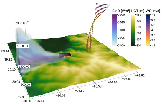
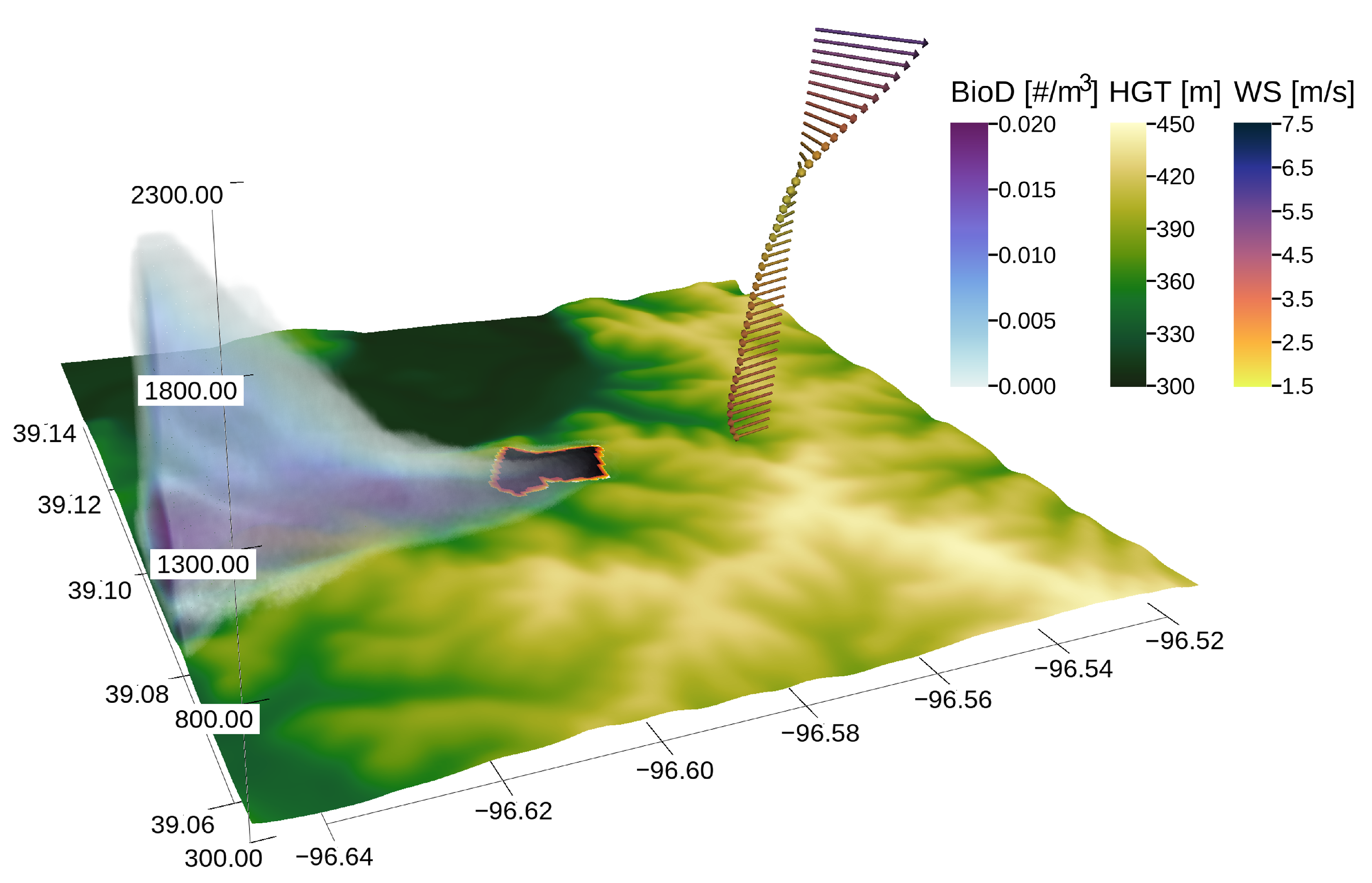
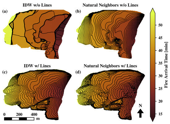
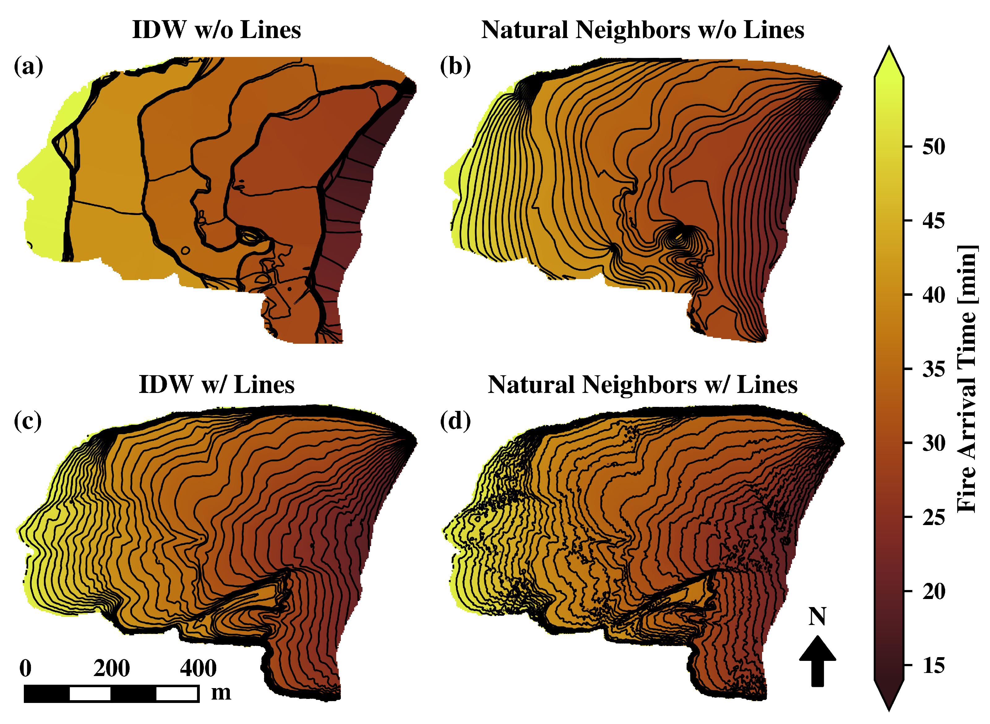
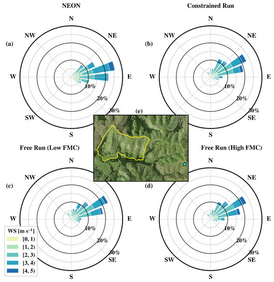
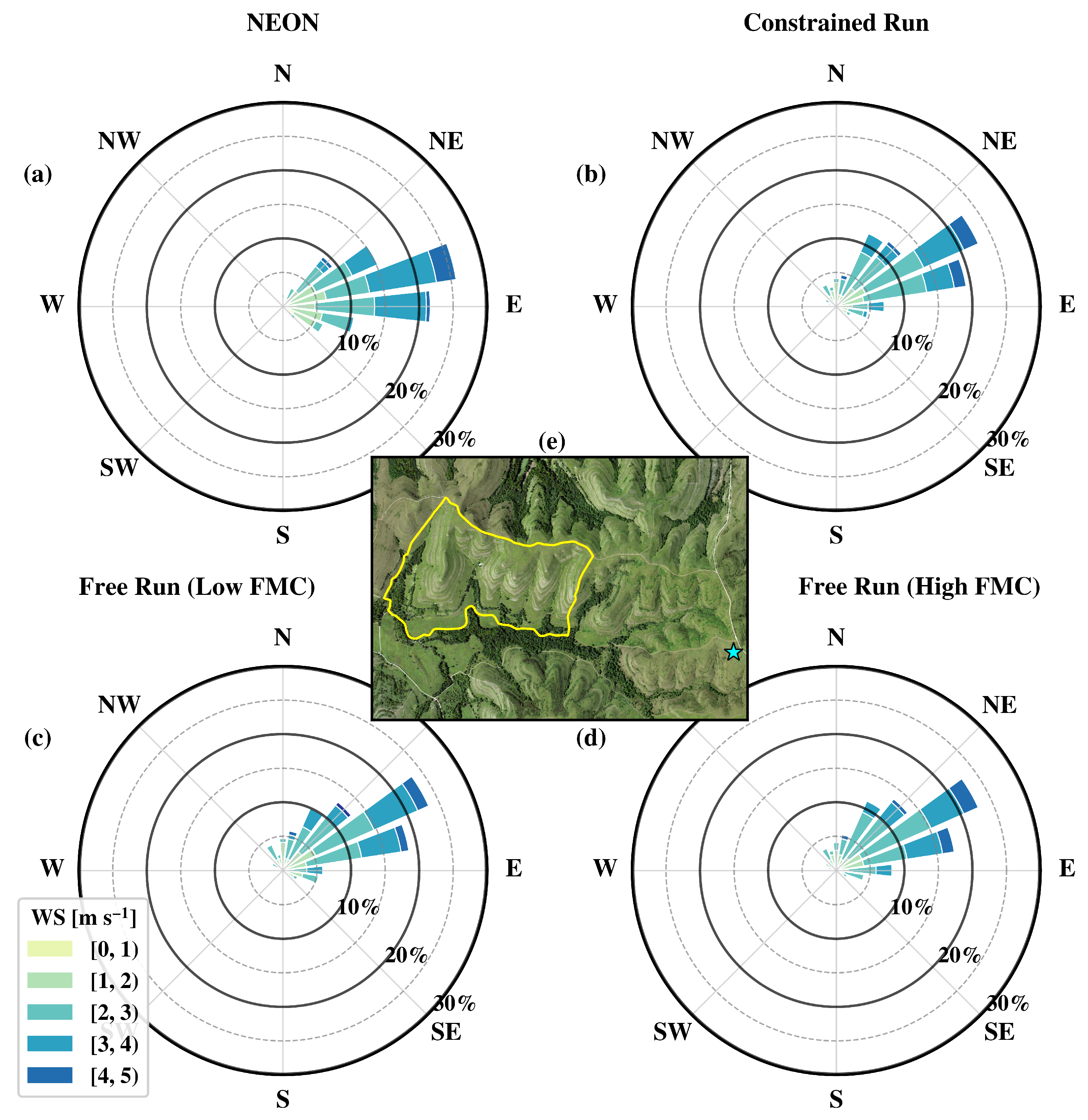
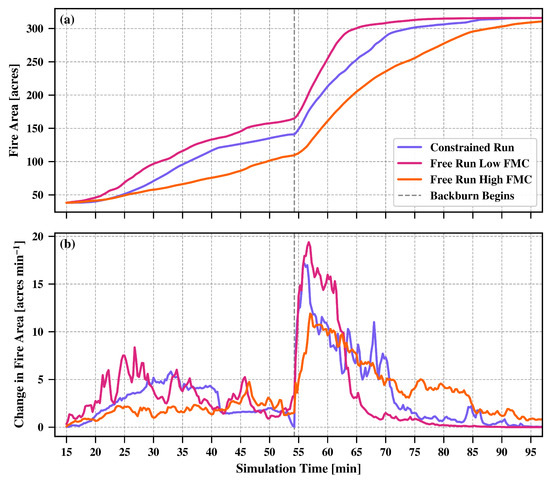
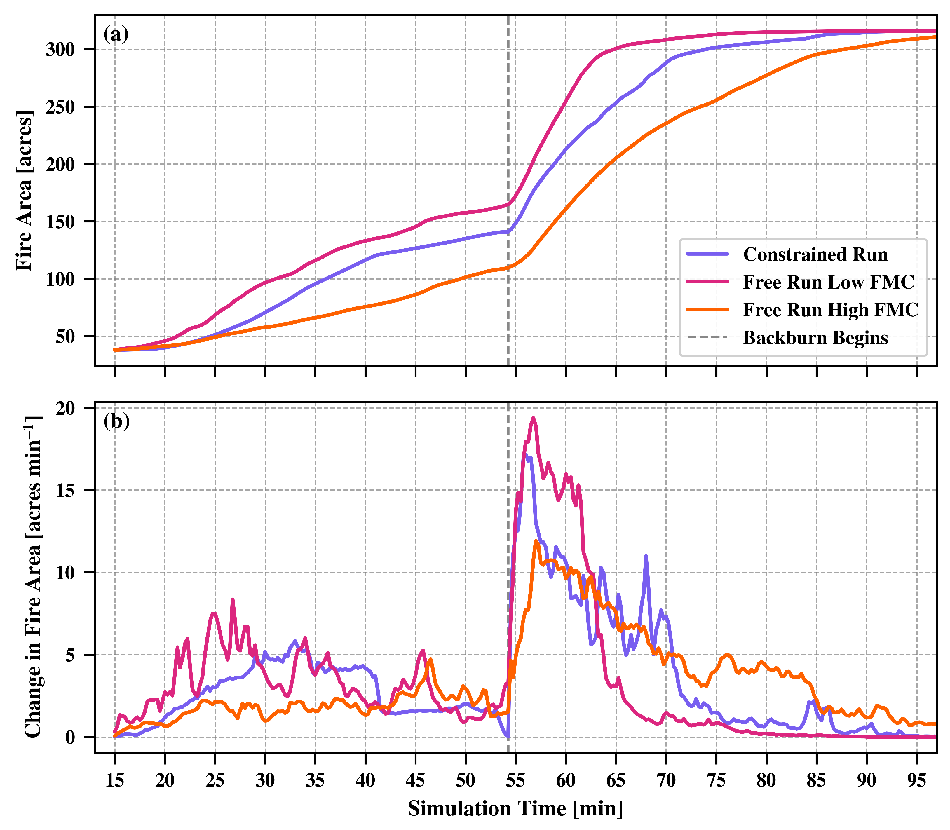
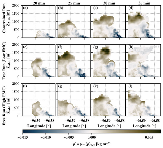
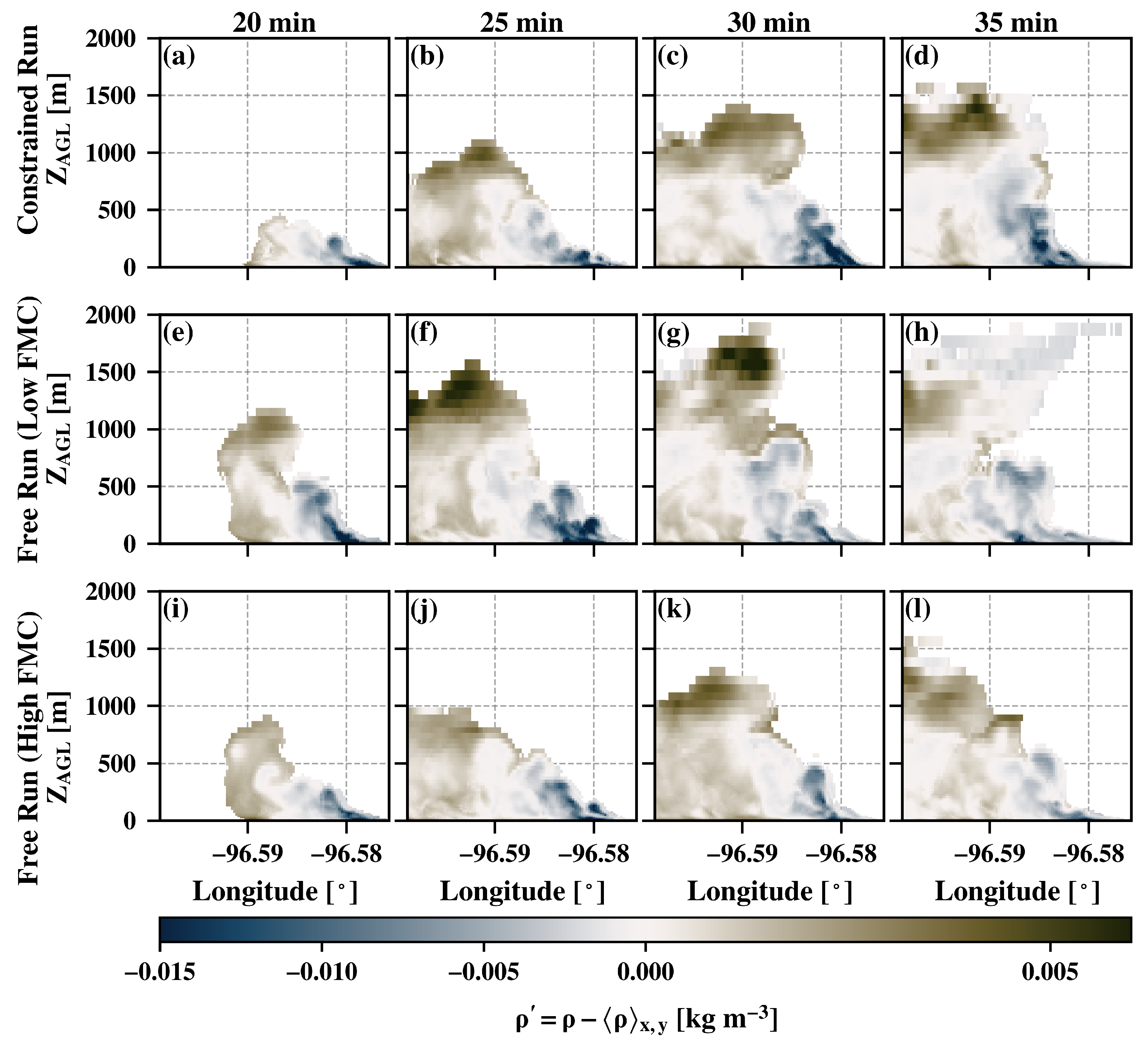
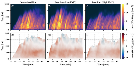
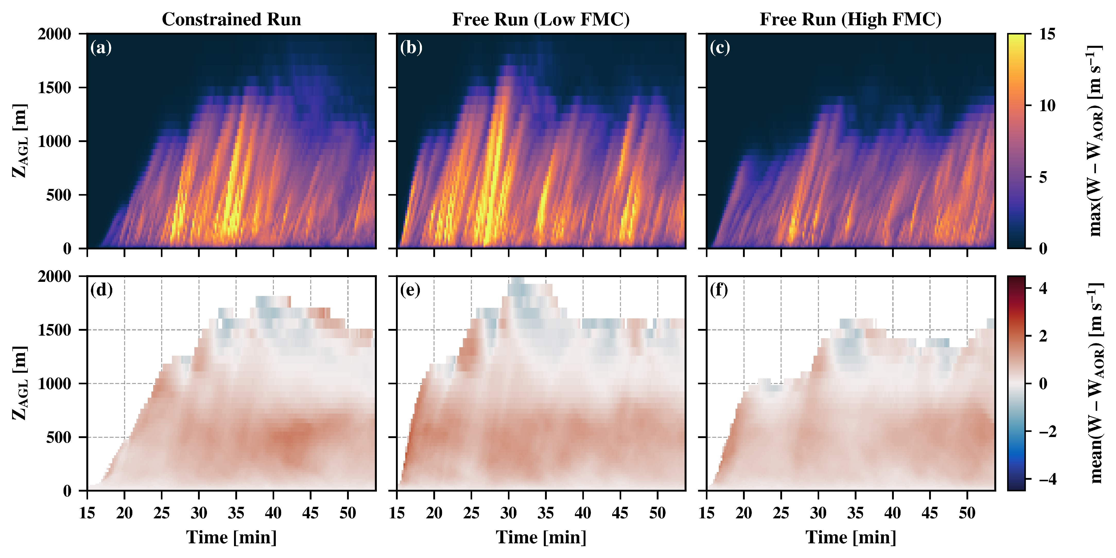
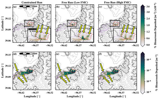
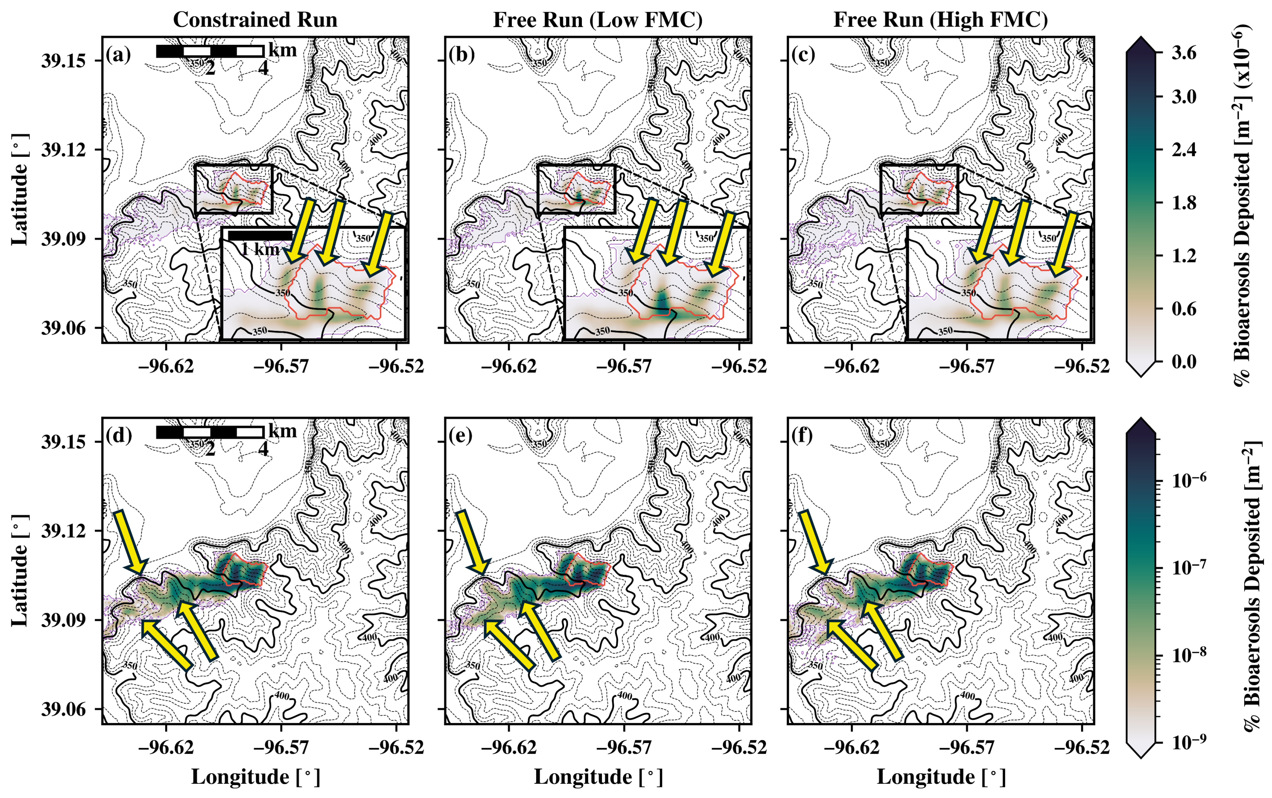
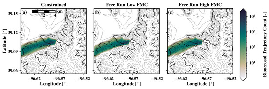
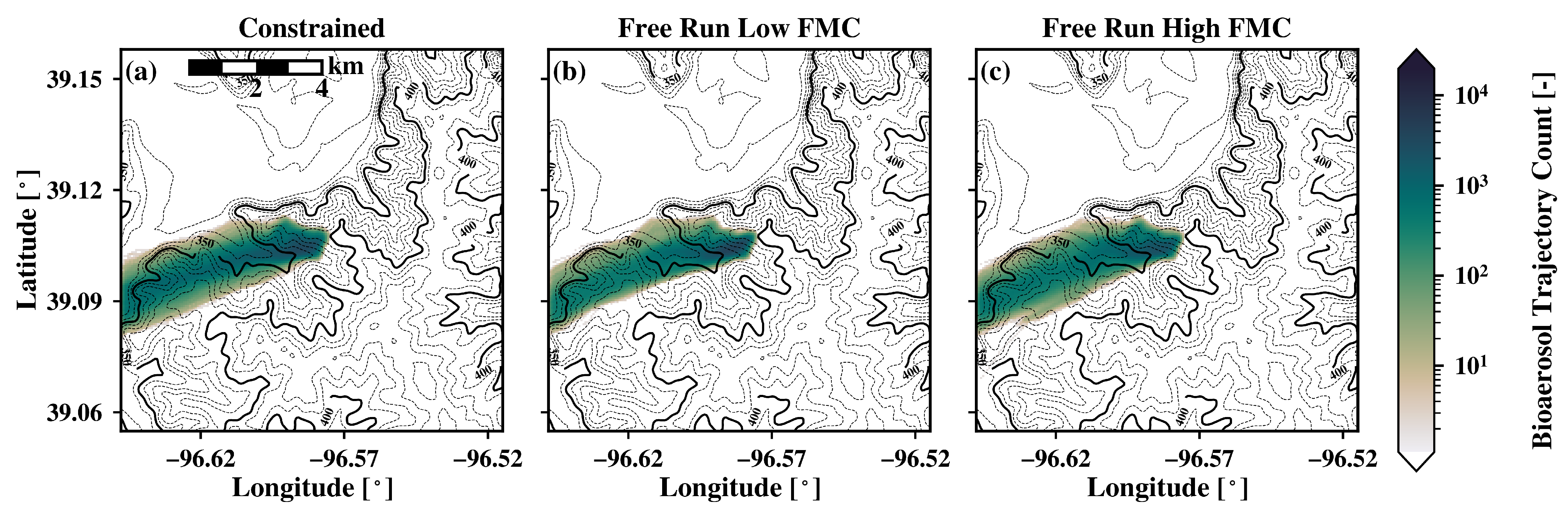
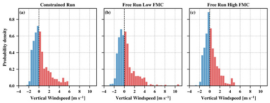
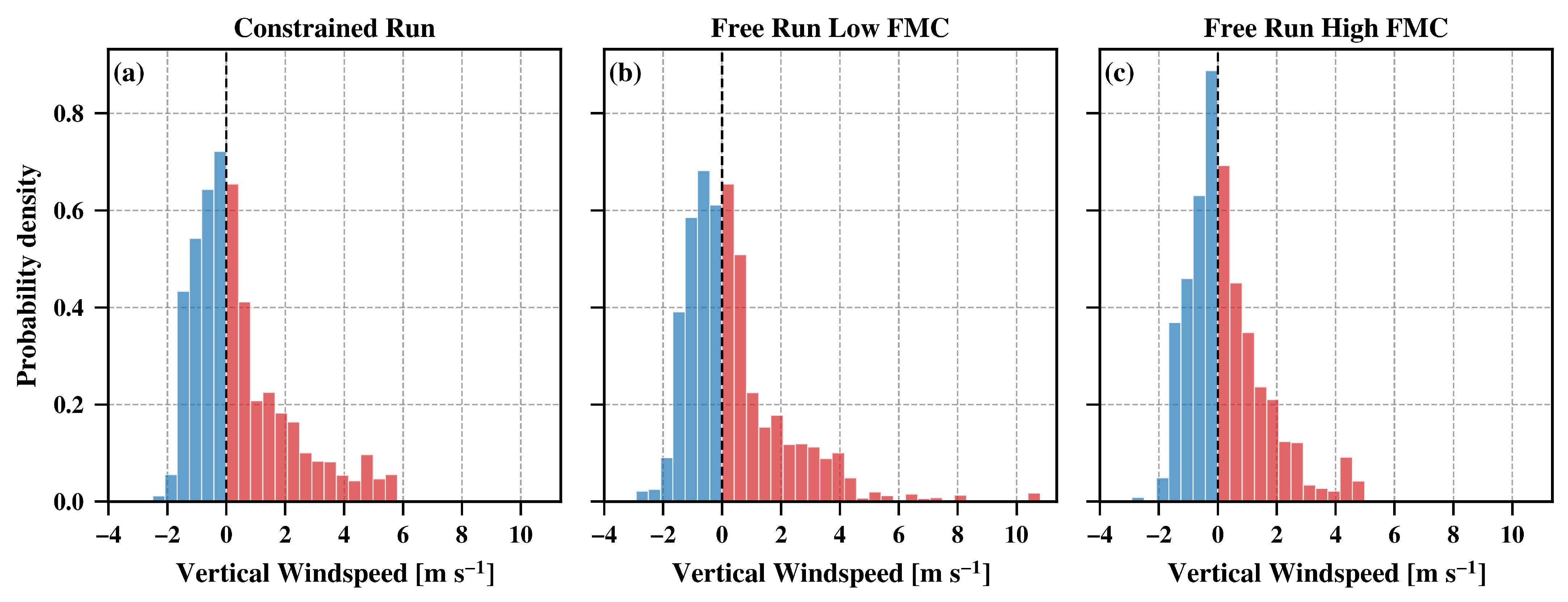

Disclaimer/Publisher’s Note: The statements, opinions and data contained in all publications are solely those of the individual author(s) and contributor(s) and not of MDPI and/or the editor(s). MDPI and/or the editor(s) disclaim responsibility for any injury to people or property resulting from any ideas, methods, instructions or products referred to in the content. |
© 2026 by the authors. Licensee MDPI, Basel, Switzerland. This article is an open access article distributed under the terms and conditions of the Creative Commons Attribution (CC BY) license.