


Highlights
What are the main findings?
- Fire severity’s relative SHAP importance declines approximately five-fold from 2021 to 2025; elevation ranks highest in 2021 and 2025, whereas pre-fire NDVI ranks highest in 2023. Complementary hotspot analysis identifies elevation-associated spatial variation in recovery.
- Annual Random Forest models, each using 15 predictors (12 common static environmental predictors and three year-specific climate predictors), failed to generalise to unseen locations under spatial cross-validation, with R2 near zero or negative across all tested spatial block resolutions, despite higher apparent performance under conventional random-split validation.
What are the implications of the main findings?
- Post-fire monitoring should be reassessed periodically, with attention to elevation-associated spatial patterns as severity-class differences narrow.
- Spatial cross-validation should become standard practice when machine learning is applied to spatially autocorrelated remotely sensed vegetation recovery data.
Abstract
The 2019–2020 Black Summer fires affected approximately 33.5% of Kosciuszko National Park, Australia’s largest alpine reserve; post-fire recovery models in Australia have rarely used spatial validation. We quantified recovery across severity classes and elevation zones (2021–2025), tested whether predictor importance shifts over time, and whether predictors generalise to unseen locations. A Sentinel-2 Normalized Difference Vegetation Index (NDVI)-derived recovery index was modelled with Random Forest at one, three and five years post-fire using 15 predictors per annual model (12 static predictors and three year-specific climate predictors) and random/spatial cross-validation; SHapley Additive exPlanations (SHAP) importance used bootstrap confidence intervals, and recovery was cross-validated against the Normalized Burn Ratio (NBR). Severity’s mean absolute SHAP importance declined from 0.116 in 2021 to 0.019 in 2025; elevation ranked highest in 2021 and 2025, whereas pre-fire NDVI ranked highest in 2023. Fast-recovery clusters occurred at lower elevation (877 versus 1284 m; p < 0.001), and montane and subalpine trajectories were statistically distinguishable. NDVI overstated recovery relative to NBR every year (p < 0.001). Spatial cross-validation R2 stayed near zero regardless of block resolution, versus 0.10–0.16 under random splitting. The association between fire severity and recovery weakened over the five-year observation period, whereas elevation-associated differences persisted; nevertheless, the annual models show limited transferability to unseen locations under spatial cross-validation. Post-fire monitoring should be reassessed periodically rather than prioritised on severity alone; spatial cross-validation should become standard for spatially autocorrelated recovery data.
1. Introduction
The 2019–2020 Australian bushfire season, popularly known as the Black Summer, burned an estimated 5.4 million hectares of New South Wales (NSW), including 2.7 million hectares of national park estate, and was the most extensive fire season in the state’s recorded history [1]. The scale of the event has been attributed to the compounding effects of record-breaking drought, extreme fuel dryness, and anomalously high spring and summer temperatures across southeastern Australia [2]. Ecological impacts were correspondingly severe, with long-unburnt fire-sensitive vegetation communities, including Gondwanan rainforest relicts, burning for the first time in recorded history in some locations. Understanding how vegetation recovers from disturbance of this magnitude and what governs the pace and completeness of that recovery is therefore central not only to post-fire land management and biodiversity conservation in the immediate term but also to anticipating ecosystem response to a fire regime that is projected to intensify in frequency and severity under continued climate change.
Remote sensing time series of spectral vegetation indices, most commonly the Normalized Difference Vegetation Index (NDVI) and the Normalized Burn Ratio (NBR), have become the standard tool for monitoring post-fire recovery at landscape scale, offering a spatially continuous and temporally repeatable alternative to labour-intensive field surveys [3]. The advent of cloud-based geospatial platforms such as Google Earth Engine [4] has made it computationally feasible to construct multi-year, cloud-free composite time series across large or remote study areas without local data storage or processing infrastructure and has substantially lowered the barrier to entry for this type of analysis. Combined with Random Forest regression [5] and, increasingly, SHapley Additive exPlanations (SHAP) [6] for interpreting the relative contribution of individual predictors, this workflow has become close to a standard template and has been applied to fire events across boreal, Mediterranean, and temperate forest systems worldwide [7].
This template has recently been applied to Australian fires specifically. A 2026 study of the 2009 Black Saturday fires in Victoria used an equivalent NDVI/NBR/Random Forest framework to show that canopy greenness (NDVI) recovered within approximately 8 years, while structural recovery (NBR) lagged, requiring around 11 years in high-severity zones [8]. This distinction matters throughout the present study: every recovery metric used here is spectral (greenness-based) rather than structural, and greenness recovery is known to outpace structural recovery and is not equivalent to biodiversity recovery in fire-affected eucalypt and snow gum ecosystems specifically [9,10]. A separate analysis of the Gospers Mountain fire, part of the same Black Summer event, used the TSS-RESTREND method to show recovery rate varied by both fire severity and land cover and that above-average post-fire rainfall accelerated recovery by an estimated two years [11]. At a global scale, an analysis of post-fire productivity recovery found post-fire climatic conditions, particularly soil moisture, vapour pressure deficit and air temperature, dominated recovery time across roughly 89% of assessed burned area worldwide, more so than pre-fire productivity or fire-induced productivity loss [12], a pattern that, if it holds locally, predicts the severity-to-climate handover this study tests directly.
A second gap this study addresses is methodological. Random Forest models of post-fire recovery are almost universally validated using random train-test splitting, yet recovery values are spatially autocorrelated by construction, since neighbouring pixels experience correlated fire behaviour, terrain and climate. Random cross-validation under these conditions systematically underestimates true predictive error, because geographically close training and test points leak information across the split even with no spatial term in the model; block-structured cross-validation, holding out spatially contiguous groups together, is recommended wherever such dependence exists [13]. None of the studies above [7,8,11,12] report spatial cross-validation, leaving open how much of their reported skill reflects genuine, transferable relationships versus spatial autocorrelation exploited by random splitting.
This study therefore has four objectives: (1) to quantify vegetation recovery trajectories across fire severity classes in Kosciuszko National Park from 2021 to 2025; (2) to use SHAP analysis of Random Forest models to test whether the relative importance of fire severity, terrain, climate, soil, and vegetation-community predictors shifts over the first five years of recovery; (3) to test, using both random and spatial block cross-validation across a range of block resolutions, whether the annual Random Forest models, each incorporating 12 common static environmental predictors and three-year-specific climate predictors, can meaningfully predict recovery at unseen locations and to situate this result within the broader methodological literature on spatial cross-validation in ecology; and (4) to test explicitly whether elevation zone, as a proxy for vegetation type and growing-season length, is associated with divergent recovery trajectories and whether these patterns persist as severity-class differences narrow.
2. Materials and Methods
2.1. Study Area
During the 2019–2020 Black Summer fire season, the Dunns Road fire and the Adaminaby fire complex (originating from the Green Valley fire) burned through the northern and central portions of the park, consuming approximately 231,000 hectares, or 33.5% of the park’s total area (Table 1) [14,15]. Burnt areas were concentrated in the montane and subalpine zones; the highest alpine areas near the park’s southern boundary, including the Thredbo and Perisher resort areas and the summit region, were largely unaffected. This uneven distribution of burnt area across the elevation gradient is a feature of the fire event itself rather than a data-processing artefact and is reflected in the spatial coverage of the fire severity data used in this study (Section 2.2), shown in Figure 1.
Table 1.
Summary of the study area and fire event.
Figure 1.
Kosciuszko National Park boundary (source: NSW National Parks and Wildlife Service Estate dataset), spanning the elevation gradient from montane eucalypt forest to subalpine snow gum woodland described above.
2.2. Fire Severity and Fire History
Fire severity for the 2019–2020 fire season was obtained from the New South Wales Fire Extent and Severity Mapping (FESM) version 3 product, a statewide 10 m raster derived from Sentinel-2 imagery using a Random Forest classifier trained on aerial photo interpretation, with five severity classes (unburnt, low, moderate, high, and extreme) plus an experimental reserved class not used operationally at the time of this study [1]. Independent aerial-photo-interpretation validation yielded balanced accuracies of 0.76–0.90 across the low-to-extreme severity classes, while post-fire field validation yielded 0.73–0.84 for the low-to-high classes; field validation for the extreme class was not reported [1]. The statewide raster was clipped to the park boundary, obtained from the NSW National Parks and Wildlife Service (NPWS) Estate dataset. Fire history back to the early twentieth century was obtained from the NSW NPWS Fire History dataset and clipped to the same boundary, and the number of previously recorded fires at each sample location was used as a predictor of fire-return-interval effects. The spatial distribution of fire severity across the park is shown in Figure 2.
Figure 2.
FESM fire severity classification for the 2019–2020 fire season, Kosciuszko National Park. White areas fall outside the fire footprint mapped by FESM.
2.3. Satellite Vegetation Indices and the Recovery Index
Sentinel-2 Level-2A surface reflectance imagery [16] was accessed via Google Earth Engine. For each year from 2019 to 2025, a cloud-masked median composite was constructed from the January–March period, chosen to hold seasonal phenology constant and avoid conflating seasonal variation with fire-driven change. From each composite, NDVI [17], NBR, the Normalized Difference Moisture Index (NDMI), and the Enhanced Vegetation Index (EVI) were calculated; NDVI was used as the primary index for the recovery calculation reported here, with NBR, NDMI, and EVI retained as ancillary indices for future cross-validation of the recovery signal.
A pixel-level recovery index was calculated for each year t from 2021 to 2025 as:
where NDVI_2019 represents pre-fire vegetation condition and NDVI_2020 represents immediate post-fire condition. A value of 1.0 indicates full recovery to pre-fire NDVI; values above 1.0 indicate NDVI exceeding the pre-fire baseline. Because this ratio is unstable where the pre/post-fire NDVI difference is small, the calculation was restricted to pixels classified as burnt (FESM severity class 2–5), and extreme outlier values were clipped to the range [−3, 3]. No additional cross-year normalisation was applied beyond the shared Sentinel-2 Level 2A surface-reflectance processing and the identical January–March compositing window used in every year, since the recovery index is defined relative to each pixel’s own pre-fire baseline rather than to a population-level annual normalisation.
Recovery_t = (NDVI_t − NDVI_2020)/(NDVI_2019 − NDVI_2020)
2.4. Environmental Predictors
Terrain variables (elevation, slope, aspect) were derived from the Copernicus GLO-30 digital elevation model (30 m). Climate variables (cumulative rainfall and mean temperature over 2020–2021, 2020–2023, and 2020–2025) were obtained from the Climate Hazards Group InfraRed Precipitation with Station data (CHIRPS) [18] and ERA5-Land [19], which also provided volumetric soil moisture for the uppermost layer (0–7 cm) over the same windows. Static soil properties (organic carbon, clay, sand, and pH, all at 0–5 cm depth) were obtained from SoilGrids 2.0 at 250 m resolution [20]. Generalised land cover came from the European Space Agency (ESA) WorldCover v200 (10 m) [21], and fine-scale vegetation community type from the NSW State Vegetation Type Map (SVTM, Extant edition; ~100 Plant Community Types (PCT) at 5 m resolution). All raster layers were accessed and pre-processed via Google Earth Engine [4] before extraction to point locations. Elevation and slope, the two topographic variables identified as most influential in subsequent analyses (Section 3.5), are mapped in Figure 3.
Figure 3.
(a) Elevation (m) and (b) slope (°) across Kosciuszko National Park, derived from the Copernicus GLO-30 digital elevation model.
2.5. Sampling Design and Dataset Construction
5000 sample points were generated within the burnt footprint, stratified to include 1250 points from each of the four FESM severity classes (low, moderate, high, extreme). At each point, the recovery index for each year (2021–2025), pre-fire NDVI, and all environmental predictors listed above were extracted. After removing points with missing values arising from edge effects at raster boundaries, 4864–4907 points remained for analysis, depending on the specific variable set used. This exclusion was not random with respect to either fire severity or pre-fire vegetation condition. Using the 5000-point pre-cleaning dataset for the full predictor and recovery variable set (4864 points retained), a chi-square test found a significant association between fire severity class and exclusion status (chi-square = 105.40, df = 3, p < 0.001): exclusion was most common among low-severity points (6.64% excluded) and least common among extreme-severity points (0.64% excluded). Excluded points also had substantially lower pre-fire NDVI than retained points (mean 0.47 versus 0.71; Mann–Whitney U test, p < 0.001). We interpret this pattern as reflecting sparsely vegetated or rocky terrain, which is both more likely to coincide with raster data gaps at mixed or boundary pixels and more likely to be mapped as low severity, since there is comparatively little canopy or understory present to register scorch. Retained severity-class proportions nonetheless remain close to the original 25% per class design (24.0% to 25.5% across the four classes), so this exclusion is unlikely to materially bias the severity-based comparisons reported throughout this study, though it does mean the sparsest, lowest pre-fire-NDVI terrain in the park is somewhat underrepresented in the analysed sample, a point we return to in Section 4.5.
2.6. Spatial Autocorrelation
Global spatial autocorrelation in the 2021 recovery values was tested using Moran’s I [22] with a k-nearest-neighbour (k = 8) row-standardised spatial weights matrix and 999 permutations. Analyses used Python 3.8.20 with the libpysal (v4.8.1) and esda (v2.5.1) packages.
2.7. Random Forest Modelling and Cross-Validation
Three Random Forest regression models (300 trees, scikit-learn v1.3.2 implementation in Python 3.8.20 [23]), a widely used ensemble method for remote sensing and environmental prediction tasks [24], were built, predicting the recovery index for 2021, 2023, and 2025, using 15 predictors, comprising 12 static environmental predictors (severity, pre-fire NDVI, elevation, slope, aspect, land cover, vegetation community (SVTM PCT), fire history count, soil organic carbon, clay, sand, and pH) and three year-specific climate predictors (rainfall, temperature, and soil moisture) corresponding to the respective recovery window. Each model was evaluated two ways, reporting both R2 and root mean square error (RMSE): (i) a conventional 80/20 random train-test split and (ii) five-fold spatial block cross-validation, in which sample points were assigned to spatial blocks using k-means clustering on point coordinates, and folds were built from held-out blocks rather than held-out points, reducing spatial dependence between training and test data relative to random splitting, following the block cross-validation approach recommended for spatially structured ecological data [13] and implemented in dedicated software such as the blockCV package [25]. To test sensitivity to the arbitrary choice of block count, the 2025 model was additionally evaluated using 5, 10, 15, 20, 30, and 50 spatial blocks, spanning coarse to fine partitions of the study area. The VIF and pairwise-correlation diagnostics reported in Section 3.2 were calculated for the 12 static predictors only. Predictor counts refer to the input variables before one-hot encoding of categorical variables.
2.8. SHAP Analysis and Uncertainty Quantification
For each of the three fitted Random Forest models, SHAP (SHapley Additive exPlanations) values were used to quantify each predictor’s contribution to model output [6], computed using the TreeExplainer implementation in the shap package (v0.44.1). The mean absolute SHAP value for each predictor was used as a measure of overall variable importance, allowing direct comparison of variable importance rankings across the three modelled years. To quantify uncertainty around these importance estimates, a bootstrap procedure was applied: for each modelled year, 20 bootstrap resamples of 2000 points were drawn with replacement, a Random Forest (100 trees) was refitted on each resample, and mean absolute SHAP values were recomputed using shap package v0.52.0 (run in a separate computing environment from the primary analysis; numpy v2.5.2, scipy v1.18.1); 95% confidence intervals were taken as the 2.5th and 97.5th percentiles of the resulting bootstrap distribution for each variable.
2.9. Cross-Index Validation with NBR
To evaluate whether the NDVI-based recovery index used throughout this study is sensitive to the choice of spectral index, an equivalent recovery index was calculated using the Normalized Burn Ratio (NBR) [26], following the identical formula, masking, and clipping procedure described in Section 2.3, using NBR calculated from the same Sentinel-2 composites. Pearson and Spearman correlations between NDVI-based and NBR-based recovery were calculated at each of the 4864 sample points for all five recovery years, and a paired t-test was used to test for systematic directional differences between the two indices.
2.10. Hotspot Analysis
Spatial clusters of significantly fast (“hotspot”) and slow (“coldspot”) recovery in 2025 were identified using the Getis-Ord Gi* local statistic [27] (esda v2.5.1 implementation), computed on the same k = 8 nearest-neighbour, row-standardised spatial weights matrix used for the Moran’s I test, with 999 conditional permutations. Self-inclusion for Gi* used esda’s default convention, with each point’s self-weight set equal to its largest neighbour weight. Points with a permutation p-value below 0.05 were classified as significant hotspots (positive z-score) or coldspots (negative z-score); all other points were classified as not significant. Mean elevation was compared across the three classes as a complementary spatial assessment of elevation-associated recovery patterns identified in the model analysis, using both Welch’s t-test and the Mann–Whitney U test to confirm the result was not dependent on distributional assumptions.
2.11. Elevation–Severity Sensitivity Analysis
An auxiliary sensitivity analysis examined whether the elevation-related model signal was sensitive to the elevation distributions of the fire-severity classes. Unlike the primary annual Random Forest models described in Section 2.7, this analysis used 21 candidate predictor variables before categorical one-hot encoding. These comprised the 12 static predictors listed in Section 2.7 and nine climate-window variables (rainfall, temperature, and soil moisture for each of 2021, 2023, and 2025). Spatial coordinates and recovery-response columns were excluded from the predictors.
Three Random Forest variants (300 trees) were fitted using an 80/20 random train–test split: (i) the full sample with all 21 candidate predictors, including severity; (ii) the subset within the common elevation range of all severity classes, also retaining all 21 candidate predictors; and (iii) the full sample with severity excluded, retaining the remaining 20 candidate predictors. Elevation permutation importance was calculated on the test set as the mean decrease in R2 when elevation values were permuted (10 repeats).
2.12. Vegetation-Community Sensitivity Analysis
To examine whether fire severity was associated with vegetation-community composition, the SVTM Plant Community Type (PCT) variable was cross-tabulated against the four severity classes. A total of 46 distinct PCT categories were identified; the ten most frequent categories were retained separately, while the remaining 36 categories were grouped as ‘Other’ for the contingency analysis. Pearson’s chi-square test of independence was used to assess the association, and Cramér’s V was calculated to describe its strength. To assess whether the observed High–Extreme recovery contrast persisted within vegetation communities, the ten most frequent PCT categories were screened for sufficient representation. Categories with at least 30 valid observations in both the High- and Extreme-severity classes were included, yielding eight eligible categories in each year. For each eligible category, High- and Extreme-severity observations were compared separately for each annual NDVI-based recovery index from 2021 to 2025 using two-sided Mann–Whitney U tests, producing 40 category-by-year comparisons. Observed group means were used to describe the direction of each contrast; because the Mann–Whitney U test assesses differences in distributions rather than means, the means were not treated as the quantity directly tested. p-values were adjusted across the 40 tests using Holm’s step-down procedure to control the family-wise error rate. These point-level analyses did not explicitly account for spatial dependence among sample locations and were therefore treated as exploratory.
3. Results
3.1. Recovery Trajectories by Fire Severity Class
Mean recovery differed clearly among severity classes in the first year post-fire, with low-severity areas closest to pre-fire NDVI (1.034) and high-severity areas furthest below it (0.722; Table 2, Figure 4). All classes rose through 2022–2023, with low- and moderate-severity areas briefly exceeding baseline. From 2023 onward, however, the ordering among severity classes broke down: by 2025, all four classes had converged to a narrow band between 0.88 and 0.92, indicating that the initial severity gradient in recovery had largely disappeared within five years.
Table 2.
Mean recovery index by fire severity class and year.
Figure 4.
Mean vegetation recovery index by fire severity class, 2021–2025. Dashed line indicates full recovery to pre-fire NDVI.
To quantify uncertainty around the severity-convergence pattern, 95% percentile bootstrap confidence intervals (2000 resamples per severity-class × year group) were calculated for the mean recovery index in each class and year (Section 3.4). The Low and Moderate intervals overlap in 2021 and 2022, while the High and Extreme intervals remain separated from the lower-severity intervals in those years. In 2023, the Low and Moderate intervals overlap, as do the Low and Extreme intervals and, marginally, the High and Extreme intervals. In 2024, the Low and High intervals overlap, as do the High and Extreme intervals. By 2025, the intervals for all four severity classes overlap pairwise. This increasing overlap is consistent with convergence in the sampled mean recovery values; however, overlap of marginal confidence intervals is descriptive and does not itself establish statistical equivalence.
3.2. Predictor Screening
Variance inflation factors (VIF) were calculated for the 12 common static environmental predictors. All VIF values were below 5, indicating no severe multicollinearity among these variables (Table 3, Figure 5). The highest VIF (4.66, clay content) reflects an expected soil-texture relationship with sand content but does not warrant exclusion of either variable. The three year-specific climate predictors were not included in this VIF screening.
Table 3.
Variance inflation factors for the environmental predictor set.
Figure 5.
Pairwise correlation matrix for the 12 static predictors (2025 model year), complementing the VIF diagnostics in Table 3.
3.3. Spatial Autocorrelation
The 2021 recovery values exhibited statistically significant positive spatial autocorrelation (Moran’s I = 0.180; expected I under the null hypothesis = −0.0002; p = 0.001; z = 27.09), confirming that recovery values are not spatially independent and that random train-test splitting is likely to overstate model performance.
3.4. Random Forest Performance: Random Split Versus Spatial Cross-Validation
The severity-class bootstrap confidence intervals discussed in Section 3.1 are summarised in Table 4(a). Random-split R2 ranged from 0.100 to 0.161 across the three modelled years, indicating weak-to-moderate apparent predictive skill. Under spatial block cross-validation, however, R2 fell to near zero or negative in every year (Table 4(b), Figure 6), indicating that the annual 15-predictor primary Random Forest models did not generalise to unseen locations despite showing weak positive skill under random splitting.
Table 4.
(a) Mean vegetation recovery index by fire severity class and year, with 95% bootstrap confidence intervals (2000 resamples). (b) Performance of the annual Random Forest models, each incorporating 15 predictors, under random-split and spatial cross-validation (20 spatial blocks).
Figure 6.
Random Forest R2 under random-split versus spatial cross-validation, by recovery year.
To test whether this gap reflected an arbitrary choice of spatial block resolution, the 2025 model was re-evaluated across six block counts (5–50). Spatial R2 remained consistently near zero or negative at every resolution tested (range: −0.146 to +0.003), well below the random-split R2 of 0.100 at every point (Figure 7), indicating the gap is a robust feature of the data rather than an artefact of one arbitrary parameter choice.
Figure 7.
Sensitivity of spatial cross-validation R2 (2025 model) to the number of spatial blocks used, compared against the random-split R2.
3.5. SHAP Variable Importance and Its Temporal Shift
SHAP analysis of the three fitted models revealed a marked temporal shift in variable importance (Table 5, Figure 8). Fire severity was the second most important predictor at year 1 (mean |SHAP| = 0.116) but declined to be among the least important predictors by year 5 (0.019), a five-fold reduction that closely mirrors the convergence of severity-class recovery trajectories described in Section 3.1. Elevation, by contrast, was the most important predictor at year 1 (0.118) and year 5 (0.106), dipping only at year 3 (0.071), making it the most temporally stable predictor in the set. Pre-fire NDVI showed a similar pattern to elevation, peaking at year 3 (0.116). Rainfall, temperature, and soil moisture for the corresponding recovery year each showed modest importance (0.02–0.03) in the year they were most relevant, consistent with a growing role for climate/moisture variables as fire severity’s relative SHAP importance declines.
Table 5.
SHAP variable importance (mean |SHAP value|) for the 15 predictors in each annual Random Forest model, comprising 12 common static predictors and three year-specific climate predictors, ranked by 2025 importance.
Figure 8.
Temporal shift in SHAP-based variable importance for the 15 predictors used in each annual Random Forest model, 2021–2025, ranked by 2025 importance.
The direction, not only the magnitude, of each variable’s effect appears in the SHAP summary plots for each year (Figure 9, Figure 10 and Figure 11). In 2021 (Figure 9), high severity (red) is associated with negative SHAP values, confirming that severely burned sites recovered more slowly, while low severity (blue) pushes predictions upward; this separation weakened by 2023 (Figure 10) and largely collapsed by 2025 (Figure 11), consistent with the declining severity importance reported above. Elevation shows a more persistent pattern: low elevation (blue) is associated with positive SHAP values in every year, while high elevation skews negative, consistent with the elevation-zone divergence in Section 3.7. Pre-fire NDVI shows the clearest direction: low pre-fire NDVI is consistently associated with negative SHAP values, indicating sparser pre-fire vegetation predicted less complete recovery.
Figure 9.
SHAP summary plot for the 2021 recovery model, showing the direction and magnitude of each predictor’s effect on model output.
Figure 10.
SHAP summary plot for the 2023 recovery model, showing the direction and magnitude of each predictor’s effect on model output.
Figure 11.
SHAP summary plot for the 2025 recovery model, showing the direction and magnitude of each predictor’s effect on model output.
To confirm that these year-to-year differences reflect genuine shifts rather than sampling noise, a bootstrap procedure (20 resamples of 2000 points per year, 100 trees per resample) was used to compute 95% confidence intervals around each mean |SHAP| estimate (Table 6, Figure 12). Severity’s confidence interval in 2021 (0.104–0.135) does not overlap at all with its 2025 interval (0.014–0.029), confirming that the decline in severity’s importance is a robust feature of the data rather than an artefact of a single model fit. Elevation’s confidence intervals show a similar pattern to Table 5’s point estimates: elevation is significantly lower at 2023 (0.057–0.095) than at 2021 (0.108–0.144), but its 2021 and 2025 (0.072–0.130) intervals overlap, indicating that while elevation’s dip at year 3 is statistically real, the claim that its importance is fully “unchanged” between year 1 and year 5 should be read as broadly stable rather than statistically identical.
Table 6.
Bootstrap 95% confidence intervals for mean |SHAP value|, selected variables (20 resamples of n = 2000 per year).
Figure 12.
Bootstrap 95% confidence intervals for SHAP-based variable importance, 2021–2025 (20 resamples of n = 2000 per year).
3.6. Cross-Validation with NBR-Based Recovery
To test whether the NDVI-based recovery index is robust to the choice of spectral index, an equivalent recovery index was calculated using NBR (Section 2.9) and compared against the NDVI-based index at all sample points for all five recovery years (Table 7, Figure 13). NDVI-based and NBR-based recovery were moderately to strongly correlated in rank order (Spearman r = 0.70–0.77 across years) but were more weakly correlated in absolute magnitude (Pearson r = 0.45–0.53), indicating that the two indices agree well on which locations recovered better than others but disagree more on the precise degree of recovery. A paired t-test at each year found that NDVI-based recovery was significantly higher than NBR-based recovery in every single year (mean difference 0.03–0.14, all p < 0.001; Table 7), consistent with the canopy-structure decoupling reported for the 2009 Black Saturday fires in Victoria, where canopy greenness (NDVI) recovered markedly faster than structural condition (NBR) [8]. The gap between the two indices was largest in 2021 and 2024 (mean difference 0.12–0.14) and smallest in 2025 (0.03), suggesting this canopy-structure decoupling is most pronounced early in recovery and narrows, though does not fully close, as structural regrowth gradually catches up to canopy greening.
Table 7.
Correlation and paired difference between NDVI-based and NBR-based recovery by year.
Figure 13.
NDVI-based versus NBR-based recovery at all sample points, 2025. Dashed line indicates 1:1 agreement; points below the line indicate NDVI overstating recovery relative to NBR.
We note that NBR is itself sensitive to soil and moisture signals, not only canopy structure, so the NDVI-NBR gap reported here should not be read as a one-sided statement that NDVI alone overstates recovery; some portion of the gap may reflect NBR’s own sensitivity to understory and soil moisture conditions rather than canopy structure specifically.
3.7. Recovery Trajectories by Elevation Zone
Stratifying sample points into montane forest (<1400 m) and subalpine woodland (1400–1850 m) revealed that the two zones followed broadly similar recovery trajectories through 2023 before diverging sharply (Table 8, Figure 14). No burnt sample points existed above 1850 m, consistent with the fire’s concentration in the park’s montane and subalpine, rather than true alpine, zone. The 95% confidence intervals around each zone’s yearly mean do not overlap at any point across 2021–2025, and the gap widens rather than narrows after 2023, indicating the two zones are statistically distinguishable throughout, not only in later stages. Subalpine woodland recovery declined from a 2023 peak of 0.957 to 0.769 by 2025, falling below its own 2021 starting value and well below full recovery. Montane forest, by contrast, declined more gently over the same period (1.020 to 0.927), remaining close to the pre-fire NDVI baseline throughout. The underlying spatial pattern of 2025 recovery, from which this elevation-zone divergence emerges, is mapped in Figure 15.
Table 8.
Mean recovery index by elevation zone and year.
Figure 14.
Vegetation recovery trajectory by elevation zone, 2021–2025, with 95% confidence bands (shaded). Bands do not overlap at any year.
Figure 15.
Spatial pattern of vegetation recovery index across Kosciuszko National Park, 2025 (values above 1.0 indicate recovery beyond pre-fire NDVI).
3.8. Hotspot Analysis
Getis-Ord Gi* analysis of 2025 recovery values identified 469 points (9.6%) as significant fast-recovery hotspots and 311 points (6.3%) as significant slow-recovery coldspots, with the remaining 4084 points (83.2%) showing no significant local clustering. Mean elevation differed substantially and in the expected direction across these three classes (Table 9, Figure 16; point counts here and throughout Section 3 follow the valid-pixel definition given in Section 2.5): hotspots occurred at a mean elevation of 877 m (s.d. 242), compared to 1284 m (s.d. 275) for coldspots. This difference was confirmed as highly statistically significant by both a parametric and a non-parametric test (Welch’s t = −21.20, p = 4.6 × 10−75; Mann–Whitney U = 19,966, p = 3.2 × 10−66), providing complementary spatial evidence of an elevation-associated pattern identified in the model analysis. The spatial distribution of these hotspot and coldspot clusters across the park is shown in Figure 17.
Table 9.
(a) Elevation permutation importance (mean decrease in test-set R2) and model test R2 under the full-sample, common-elevation-band, and severity-excluded auxiliary model variants by year. (b) Elevation of recovery hotspot and coldspot clusters, 2025 (Getis-Ord Gi*, k = 8, 999 permutations). Hotspot versus coldspot elevation differed significantly (Welch’s t = −21.20, p = 4.6 × 10−75; Mann–Whitney U = 19,966, p = 3.2 × 10−66).
Figure 16.
Mean elevation (±1 s.d.) of significant recovery hotspot, coldspot, and non-significant clusters, 2025.
Figure 17.
Spatial distribution of significant recovery hotspots and coldspots, 2025, identified by local Getis-Ord Gi* statistics.
3.9. Sensitivity Analyses for Elevation and Vegetation-Community Composition
Figure 18 maps the spatial distribution of fire severity class (panel a) and elevation (panel b) across all sample points and summarises the resulting severity-class composition within the two elevation zones defined in Table 8 (panel c). The composition differs between zones: in the montane forest zone, Low, Moderate and High severity points occur in broadly similar proportions (27.1%, 27.3% and 27.9%, respectively), with Extreme severity comparatively underrepresented (17.7%), whereas in the subalpine woodland zone, Extreme severity accounts for the largest single share of points (49.3%), nearly double its montane-zone share, while Low severity falls to its smallest share in either zone (14.5%).
Figure 18.
Spatial distribution of fire severity class (a) and elevation (b) across all sample points, and severity-class composition within the montane forest and subalpine woodland elevation zones (c).
Because elevation and fire severity are not assigned independently across the landscape, we tested directly whether the elevation–recovery association reported above is an artefact of this confound. Elevation differed significantly across the four severity classes (Kruskal–Wallis H = 321.00, p = 2.83 × 10−69), although the associated effect size was small-to-moderate (ε2 = 0.065), indicating that despite the extreme significance driven by the large sample size, severity classes overlap substantially in elevation rather than occupying wholly separate elevation bands. Restricting the dataset to the elevation range common to all four severity classes (392.6–1717.9 m) retained 4848 of 4864 points (99.7%), confirming that the severity classes are not confined to disjoint elevation zones.
Table 9(a) reports elevation permutation importance (mean decrease in test-set R2 when elevation values are permuted) and the corresponding test R2 under three auxiliary model variants fitted separately for 2021, 2023, and 2025. These auxiliary models used 21 candidate predictors before categorical one-hot encoding: the 12 static predictors and nine climate-window variables described in Section 2.11. The three variants comprised the full sample with severity included, the common-elevation-band subset with severity included, and the full sample with severity excluded. Elevation permutation importance was retained and increased under the overlap-band restriction and severity exclusion in all three target years. These results suggest that the elevation-associated model signal is not explained solely by unequal elevation distributions across severity classes, but they do not establish a causal or fully independent elevation effect.
A further sensitivity analysis examined whether the observed High–Extreme recovery contrast was associated with differences in vegetation-community composition among fire-severity classes. The contingency analysis showed a statistically significant association between fire severity and SVTM Plant Community Type (PCT) composition (χ2(30, N = 4864) = 1179.59, p = 5.18 × 10−229; Cramér’s V = 0.284). The ten most frequent PCT categories accounted for 76.4% of the sample points; the remaining 36 categories were grouped as ‘Other’ for this test. Within-community comparisons were conducted for the eight PCT categories with at least 30 valid observations in both the High- and Extreme-severity classes, yielding 40 two-sided Mann–Whitney U tests across the five recovery years. Before adjustment, 19 of the 40 comparisons were significant at p < 0.05; in all 19, the observed mean NDVI recovery was higher in Extreme- than in High-severity pixels. None showed a significant difference in the opposite direction. After Holm adjustment across all 40 comparisons, nine remained statistically significant, all in the same direction. Thus, the High–Extreme recovery reversal persisted within a subset of the sampled PCT categories, but most category-by-year comparisons were not significant after adjustment. These results do not support the claim that vegetation-community composition alone explains the pooled High–Extreme reversal, nor do they quantify the contribution of PCT composition to the pooled severity-class differences. Because the tests used point-level observations without explicitly accounting for spatial dependence, these findings should be interpreted as exploratory.
4. Discussion
4.1. The Association Between Fire Severity and Recovery Weakens over Time
The clearest pattern in the results is that the association between fire severity and recovery was strongest in the first post-fire year and weakened over the five-year observation period. Severity strongly separated recovery trajectories at one year post-fire in both the descriptive comparison (Table 2) and SHAP-based importance (Table 5), with a roughly five-fold decline between 2021 (0.116) and 2025 (0.019). This is consistent with the Gospers Mountain TSS-RESTREND analysis, which similarly found severity-dependent differences that narrowed as post-fire rainfall accumulated [11], and with the global analysis of Xu et al. (2024) [12], which found post-fire climatic conditions dominated recovery time across most global burned areas, exceeding pre-fire productivity and fire-induced productivity loss once the acute phase had passed. Our results extend this by quantifying the shift within a single modelling framework and showing that the relative importance of fire severity declines, while climate- and moisture-related predictors become more prominent, between roughly the first and third post-fire years in the sampled communities.
Three complementary lines of evidence help explain why this convergence occurs so consistently. First, above-average rainfall during the La Niña-influenced 2021–2023 period in south-eastern Australia is a plausible driver of accelerated recovery in the initially most severely burnt plots, consistent with the rainfall-driven acceleration of severity-dependent recovery documented at Gospers Mountain [11]. Second, NDVI is known to saturate at moderate-to-high canopy cover [8,28], which compresses the attainable range of the recovery index as vegetation re-greens and mechanically narrows the gap between severity classes over time regardless of the underlying ecological process. Third, the vegetation-community sensitivity analysis in Section 3.9 indicates that the High–Extreme recovery reversal is not uniform across PCT categories. Nineteen of the 40 within-PCT comparisons were nominally significant before adjustment, but only nine remained significant after Holm correction; all nine showed a higher observed mean NDVI recovery in Extreme- than in High-severity pixels. The remaining comparisons were not significant after adjustment. Thus, the reversal persists within a subset of the sampled PCT categories, but these results do not quantify the contribution of vegetation-community composition to the pooled severity-class pattern or establish an independent causal effect of severity.
4.2. Elevation-Associated Patterns and Temporal Predictor Importance
Elevation showed a temporally persistent pattern of model-based importance, ranking highest in 2021 and 2025 and below pre-fire NDVI in the 2023 model. The 2025 hotspot analysis also identified fast-recovery clusters at a lower mean elevation than slow-recovery coldspots (877 m versus 1284 m; Table 9). This spatial pattern provides complementary evidence of elevation-associated variation in recovery. The agreement between model-based importance and hotspot patterns is informative, but neither analysis establishes a causal elevation effect nor demonstrates independence from other environmental gradients.
We interpret the elevation association as potentially reflecting its relationship with post-fire climatic and microclimatic conditions, including temperature, frost frequency, snow persistence, and soil moisture, rather than as a direct causal mechanism of its own. This interpretation is consistent with Xu et al. (2024), whose global analysis found post-fire climatic variables dominated recovery time across 91% of burned area once the acute severity-driven phase had passed [12], and with Zahura et al. (2024), who found topographic and climate variables jointly outperformed severity and land-cover variables in predicting post-fire recovery trajectories [7]. The primary models included year-specific gridded rainfall, temperature, and near-surface soil-moisture predictors. These landscape-scale summaries do not, however, resolve fine-scale microclimatic conditions, frost frequency, snow persistence, or local soil-water dynamics. Elevation may therefore retain information about environmental gradients not fully represented by the available gridded climate variables; the comparatively low spatial-CV R2 reported throughout this study (Section 4.3) is consistent with the limited ability of the available predictors to explain recovery at unseen locations. This snow-persistence pathway specifically is supported by independent climatological evidence from this same region, where precipitation falls predominantly as snow above approximately 1400 m [29], closely matching the montane–subalpine elevation threshold used throughout this study (Table 8). A second, independently verified source specific to this same range reports that snow cover remains present across every observed year specifically above approximately 1500 m in the Snowy Mountains [30], reinforcing the same montane-to-subalpine threshold from an independent dataset and analytical method. Quantitative support for the growing-season part of this mechanism comes from the Victorian Alps, part of the same broader Australian alpine bioregion: early-melting snowpatches at 1670 to 1850 m average 23 to 53 snow days into the growing season, compared with 53 to 83 snow days at sites above 1850 m, a documented elevation-linked difference in how much growing season late-lying snow removes [31]. A direct, New South Wales-specific source for the growing-season and frost pathways is the classic account by Costin [32], who reports that mean monthly minimum temperature remains below freezing for approximately six months of the year in the subalpine tract (between the snow line and treeline) and six to eight months in the alpine tract (above treeline) in this region, with the snow line at approximately 1520 to 1680 m and treeline at approximately 1680 to 1980 m in New South Wales and the Australian Capital Territory, elevations that sit directly across the montane and subalpine thresholds used in this study (Table 8). This directly supports the frost-frequency and growing-season part of the proposed mechanism for this specific region, with the Victorian snow-day comparison above [31] as corroborating quantitative context from the same broader bioregion.
The persistence of pre-fire NDVI as an important predictor, particularly at year 3 (SHAP = 0.116, the highest value in the 2023 model), is consistent with ecological memory, whereby the legacy of pre-disturbance ecosystem state shapes post-disturbance trajectories independently of the disturbance event itself [33]. Under this interpretation, sites with denser, more vigorous pre-fire vegetation retain greater capacity for recovery: at lower fire severity, eucalypts commonly resprout epicormically from surviving stems [34], whereas more severely burnt stems draw on root and lignotuber reserves and local seed banks as an information and material legacy, consistent with lignotuber-based vegetative recovery documented in Kosciuszko snow gum one year after the 2003 fires [35]. Sites with greater pre-fire vegetation density and vigour therefore recover more readily and rapidly once the initial post-fire growth phase is underway. This is consistent with the broader concept of ecological memory introduced above, in which antecedent ecosystem state measurably, and sometimes underappreciably, shapes disturbance recovery trajectories.
This ecological-memory interpretation should, however, be read with an important caveat. A SHAP sensitivity analysis comparing random-split and spatial block cross-validation found that pre-fire NDVI’s importance was concentrated specifically in the 2023 model and fell by roughly two-thirds (68.5%) once spatial block cross-validation was used instead of a random split, indicating this particular predictor’s apparent importance is substantially more sensitive to the validation scheme and study year than elevation’s. We therefore present the ecological-memory interpretation above as most strongly supported for 2023 under random-split evaluation, rather than as a uniformly robust effect across every year and validation scheme tested.
The persistent elevation-associated pattern is also consistent with the statistically distinct late-stage decline identified in subalpine snow gum woodland (Section 3.7). Beyond the climatic mechanism proposed above, the within-PCT analysis in Section 3.9 indicates that the High–Extreme recovery contrast varies among vegetation communities: nine of the 40 category-by-year comparisons remained significant after Holm adjustment, and all showed a higher observed mean NDVI recovery in Extreme- than in High-severity pixels. This analysis does not, however, establish that vegetation-community composition explains the late-stage decline in subalpine snow gum woodland. Independently, high-elevation snow gum woodland in this park has been documented to experience elevation-associated dieback driven by Phoracantha beetle infestation [36], a stressor unrelated to the 2019–2020 fires but concentrated in the same high-elevation zone. We cannot fully separate a climate-proxy mechanism from a vegetation-community-specific vulnerability mechanism with the present predictor set and recommend this be tested directly in future work using explicit, fine-grained vegetation-type classification (e.g., distinguishing snow gum woodland from other subalpine and montane classes) rather than the coarser community categories used here.
4.3. Limited Spatial Predictability and Its Implications for the Field
The most methodologically important finding of this study, however, is the consistent failure of the 15-predictor primary Random Forest models, spanning fire severity and history, terrain, climate, soil physicochemical properties, and fine-scale vegetation community type, to generalise under spatial cross-validation, regardless of the spatial block resolution used to define the cross-validation folds (Section 3.4, Figure 7). This has at least two distinct implications, one ecological and one methodological.
Ecologically, it suggests that recovery at any location retains a meaningful component not explained by any combination of the variables tested, even though several (severity, elevation, pre-fire NDVI) show clear relationships with recovery in aggregate: these variables shift the distribution of likely outcomes without narrowing it enough for confident pixel-level prediction. The unexplained variance may reflect fine-scale processes below the resolution of the data used here, including microtopographic variation in soil moisture and frost exposure, localised seed dispersal and recruitment limitation, patchy herbivory, or individual weather events during the critical early resprouting window. Feral horse grazing and trampling is a plausible source of this patchy variance: feral horses cause extensive, spatially uneven damage to vegetation, soil and waterways across Kosciuszko and the broader Australian Alps, concentrated in particular sub-catchments rather than distributed evenly [37]. A paired comparison of Sphagnum peatland sites within the park found that sites with feral horse presence were net carbon sources, while similar sites without horses were net carbon sinks [38], a site-to-site difference driven by an unmapped biotic disturbance that none of the 15 predictors in the primary models were designed to capture.
We emphasise that near-zero or negative spatial-CV R2 alongside clear, consistent SHAP relationships under random-split evaluation (Section 3.4 and Section 3.5) is not a contradiction. The random-split SHAP values describe associations the model exploited where training and held-out points share spatial neighbours and, by extension, unobserved local conditions; the spatial-CV R2 instead tests whether those same associations transfer to locations with no nearby training data. The consistent loss of skill across every block count tested, from the finest to the coarsest resolution (Figure 7), argues against this being an artefact of any single, arbitrarily chosen block size, and supports treating the two metrics as answering different questions rather than as disagreeing with one another.
Methodologically, this result is a caution for the broader post-fire recovery literature. Block cross-validation, or an equivalent method respecting spatial dependence, should be used wherever such structure exists, even where no correlation is visible in fitted model residuals [13]. This pattern is not unique to post-fire recovery: an analogous demonstration in large-scale tropical forest biomass mapping found a model explaining over half of the variance under random validation showed quasi-null predictive power once spatial autocorrelation was accounted for [39]. None of the directly comparable Australian or global post-fire recovery studies discussed here [7,8,11,12] report spatial cross-validation alongside random-split metrics, despite recovery values being spatially autocorrelated by construction in every case, a property we confirmed for our own study area via Moran’s I (Section 3.3). The gap identified here, roughly 0.10–0.25 R2 units, and its consistency across a six-fold range of block counts (Figure 7) suggest that predictive skill based solely on random splitting may be optimistic when strong spatial dependence is present, as it likely is in comparable published studies that do not report spatial cross-validation. We recommend that spatial cross-validation, or at minimum an explicit report of spatial autocorrelation, become standard practice when Random Forest methods are applied to spatially continuous ecological outcomes.
4.4. Implications for Post-Fire Land Management
From a management perspective, these results offer two practical points. First, the rapid convergence of severity-class recovery by year 3–5 suggests initial burn severity is a comparatively poor long-term indicator of which locations need sustained management attention; sites should instead be re-assessed periodically, since a site severely affected in year 1 may show no meaningful difference from a lightly burned site by year 3. Second, the persistent elevation-associated spatial pattern and late-stage subalpine decline suggest post-fire monitoring and intervention (such as feral herbivore control or supplementary planting) may be more usefully prioritised toward higher-elevation burned areas from around year 3 onward, when the divergence from lower-elevation forest becomes apparent, rather than allocated primarily on initial severity mapping.
4.5. Limitations and Future Directions
This study has several limitations. First, the FESM severity product covers approximately half the park’s area; the unmapped remainder was unburnt higher-elevation terrain, meaning recovery could not be assessed above ~1850 m. This coverage gap reflects where the 2019–2020 fires actually burned, rather than a flaw or omission in the FESM product itself, since FESM maps severity only within the mapped fire perimeter. Second, this is a single-park, remote-sensing-only study without direct field validation; related field-based studies exist for this park for other vegetation types [40,41], and we treat the present findings as hypothesis-generating rather than confirmatory, offering specific testable predictions such as field-measured resprouting vigour decoupling from canopy NDVI recovery in high-severity subalpine plots by year 3–5. Third, NDVI systematically overstated recovery relative to NBR in every year (Section 3.6), consistent with known NDVI saturation in dense canopy [8,28]; NDMI and EVI composites remain available for further cross-index validation. Finally, the five-year study window captures only the early phase of what is likely a multi-decadal recovery process for slower-growing subalpine communities, and continued monitoring will be needed to confirm whether the late-stage subalpine decline identified here persists or eventually re-converges with montane forest.
Beyond these limitations, several alternative approaches to quantifying post-fire vegetation recovery warrant consideration, particularly NBR2-based recovery measures, delayed or rolling recovery indices, and recovery classification schemes. These approaches have been applied to Australian, and specifically New South Wales, post-fire recovery monitoring using comparable Sentinel-2 or Landsat time series [42,43]. NBR2 substitutes two shortwave-infrared bands for the near-infrared and shortwave-infrared pairing used in standard NBR. In a New South Wales case study spanning ten fires, including several from the 2019–2020 Black Summer, an NBR2-based post-fire stability index was the best supported single predictor of three of four field-measured recovery responses, and the only candidate index among NBR, NBR2, and their pre-fire-baseline and post-fire-stability variants able to statistically separate low- from moderate-severity recovery [42]. We did not adopt NBR2 here. This study already cross-validates its primary NDVI-based recovery signal against standard NBR (Section 2.9 and Section 3.6), and extending that comparison to NBR2 specifically was outside the present scope but is a reasonable next step given the result reported [42].
The same New South Wales study introduced a delayed, rolling recovery index that compares each post-fire year’s spectral value against the immediately preceding year, rather than against a single pre-fire baseline, specifically to avoid the instability a fixed pre-fire baseline can introduce when pre-fire years are affected by drought or other anomalous rainfall [42]. This differs from the fixed, 2019 pre-fire baseline design used throughout the present study (Section 2.3). We retained a fixed baseline here for direct comparability with the global and Australian NDVI- and NBR-based studies discussed throughout this Discussion [7,8,11,12], while recognising that a delayed or rolling baseline is a methodologically distinct, and in some settings more robust, alternative worth testing against the present dataset in future work. A second New South Wales Black Summer study, using standard NBR with a fixed one-year post-fire baseline, similarly reported that the effect of severity on spectral recovery varied regionally, weak in the north-east and markedly stronger in the south [43], a pattern broadly consistent with the spatially uneven, elevation-mediated recovery reported here (Section 4.1, Section 4.2 and Section 4.3).
Recovery classification approaches summarise a continuous recovery signal into a small number of discrete, interpretable states, rather than reporting the continuous value itself. The New South Wales post-fire stability index is itself converted into a standardised thirteen-class scheme, from extreme decrease to extreme increase, to characterise system stability at each post-fire time step [42], and the widely used LandTrendr algorithm segments a pixel’s spectral trajectory into disturbance, recovery, and stable segments on a related conceptual basis [44]. We did not adopt a classification approach here because this study’s central aim, quantifying how much fire severity and elevation explain variation in recovery via Random Forest and SHAP (Section 2.6, Section 2.7 and Section 2.8), required a continuous response variable. Translating the present recovery index into a small number of discrete classes, as in [42,44], is a natural extension for future work and may be of particular value for operational monitoring contexts where a small number of interpretable states is preferable to a continuous index.
Several further limitations should be noted. The fire-history predictor used here was a simple count of recorded fires at each location; we did not have access to time-since-previous-fire, inter-fire interval, or fire-season timing data, any of which could carry independent explanatory value not captured by a count alone. This study also examines recovery from a single fire event, and the generalisability of the specific findings reported here, particularly the roughly three-year severity-convergence window, to other fire events, regions, or ecosystems remains to be tested. The Sentinel-2 composites used throughout may also retain some residual atmospheric contamination (haze, thin cloud, or smoke) despite cloud masking, which could not be fully excluded at this spatial and temporal resolution. The point exclusions described in Section 2.5 were also not random: exclusion was significantly more common among low-severity, low-pre-fire-NDVI locations than among higher-severity locations, plausibly reflecting sparsely vegetated or rocky terrain that is both prone to raster data gaps and likely to register as low severity. Retained severity-class proportions remain close to the original 25% per class design, so this is unlikely to materially bias the severity-based comparisons reported throughout this study, but it does mean the sparsest, lowest pre-fire-NDVI terrain in the park is somewhat underrepresented in the analysed sample. Additionally, the vegetation-community sensitivity analysis in Section 3.9 was based on point-level contingency and within-PCT tests that did not explicitly model spatial dependence among sample locations. Although Holm adjustment controls the family-wise error rate across the 40 within-PCT comparisons, it does not account for spatial autocorrelation; these results should therefore be interpreted as exploratory. Finally, the January–March compositing window, while applied identically and consistently across every study year to preserve comparability, is itself an arbitrary choice among several defensible alternatives, and results using a different fixed seasonal window were not tested here.
5. Conclusions
Vegetation recovery following the 2019–2020 Black Summer fires in Kosciuszko National Park shows a temporal shift in model-based predictor importance: fire severity had relatively high importance in the first post-fire year but declined substantially by 2025, while elevation ranked highest in the 2021 and 2025 models and pre-fire NDVI ranked highest in 2023. The 2025 hotspot analysis also identified fast-recovery clusters at lower mean elevations than slow-recovery coldspots, providing complementary evidence of elevation-associated spatial variation; these model-based and spatial associations should not be interpreted as causal effects. A cross-index comparison further showed that NDVI-based recovery estimates exceeded NBR-based estimates in every year, indicating that canopy greenness and the spectral signal captured by NBR do not track identically. The 15-predictor primary Random Forest models (12 static predictors and three year-specific climate predictors) did not generalise reliably to unseen locations under spatial cross-validation, despite positive R2 under random splitting. Overall, the results indicate that recovery patterns are associated with changing severity-class differences, elevation-related environmental gradients, and variation in the High–Extreme recovery contrast among the sampled PCT categories in a landscape also affected by regional climate [29], documented high-elevation dieback [36], and reburn-related stressors. We recommend that future Random Forest-based post-fire recovery studies routinely report spatial, in addition to random, cross-validation results and bootstrap-based uncertainty. Alpine and subalpine systems, several of which are classified as threatened by climate- and fire-regime-driven risk assessments [45], warrant further targeted investigation given the late-stage recovery divergence identified here.
Author Contributions
Conceptualization, O.Z.A.M. and N.S.; methodology, O.Z.A.M. and N.S.; software, O.Z.A.M. and N.S.; validation, O.Z.A.M., N.S. and Z.K.; formal analysis, O.Z.A.M. and N.S.; investigation, O.Z.A.M. and N.S.; resources, H.L.; data curation, O.Z.A.M. and N.S.; writing—original draft preparation, O.Z.A.M. and N.S.; writing—review and editing, N.S., Z.K. and H.L.; visualization, O.Z.A.M.; supervision, H.L.; project administration, H.L. All authors have read and agreed to the published version of the manuscript.
Funding
This research received no external funding.
Institutional Review Board Statement
Not applicable. This study involved no human participants or animal experimentation; it used remote-sensing and other publicly available spatial datasets.
Informed Consent Statement
Not applicable.
Data Availability Statement
All primary datasets used in this study are publicly available. The NSW Fire Extent and Severity Mapping (FESM), NSW Fire History, NPWS Estate boundary and NSW State Vegetation Type Map datasets are freely available from the NSW Government SEED portal (https://www.seed.nsw.gov.au, accessed on 28 August 2026). Sentinel-2 Level-2A surface reflectance imagery, the Copernicus GLO-30 digital elevation model, CHIRPS precipitation data, ERA5-Land climate and soil moisture data, and ESA WorldCover land cover data were accessed via Google Earth Engine (https://earthengine.google.com, accessed on 28 August 2026). SoilGrids 2.0 data are available from the International Soil Reference and Information Centre (ISRIC) (https://soilgrids.org, accessed on 28 August 2026). The derived recovery rasters, the sample point dataset and the analysis code generated during this study are available from the corresponding author upon reasonable request.
Acknowledgments
We acknowledge the Traditional Owners and Custodians of the lands on which this research was conducted, the Monaro Ngarigo, Wiradjuri, Wolgalu and Ngunnawal peoples, as recognised in the Kosciuszko National Park Plan of Management (NSW Department of Climate Change, Energy, the Environment and Water), and pay respect to their Elders past and present, and to their continuing cultural and spiritual connection to the mountains and waterways of the Australian Alps. We thank the NSW Department of Climate Change, Energy, the Environment and Water for maintaining and freely distributing the FESM, Fire History, NPWS Estate and SVTM datasets used in this study, and the Google Earth Engine development team for providing free access to the computational platform on which the satellite-derived predictors were processed.
Conflicts of Interest
The authors declare no conflicts of interest.
Abbreviations
The following abbreviations are used in this manuscript:
| NDVI | Normalized Difference Vegetation Index |
| NBR | Normalized Burn Ratio |
| NDMI | Normalized Difference Moisture Index |
| EVI | Enhanced Vegetation Index |
| SHAP | SHapley Additive exPlanations |
| RMSE | Root Mean Square Error |
| VIF | Variance Inflation Factor |
| CI | Confidence Interval |
| FESM | Fire Extent and Severity Mapping |
| NPWS | NSW National Parks and Wildlife Service |
| SVTM | State Vegetation Type Map |
| PCT | Plant Community Type |
| CHIRPS | Climate Hazards Group InfraRed Precipitation with Station data |
| ERA5 | ECMWF Reanalysis v5 |
| DEM | Digital Elevation Model |
| s.d. | standard deviation |
References
- NSW Department of Planning and Environment. DPE Fire Extent and Severity Mapping (FESMv3) Factsheet; NSW Government: Sydney, NSW, Australia, 2020.
- Nolan, R.H.; Boer, M.M.; Collins, L.; Resco de Dios, V.; Clarke, H.; Jenkins, M.; Kenny, B.; Bradstock, R.A. Causes and consequences of eastern Australia’s 2019–20 season of mega-fires. Glob. Change Biol. 2020, 26, 1039–1041. [Google Scholar] [CrossRef] [Scilit] [PubMed]
- Bright, B.C.; Hudak, A.T.; Kennedy, R.E.; Braaten, J.D.; Henareh Khalyani, A. Examining post-fire vegetation recovery with Landsat time series analysis in three western North American forest types. Fire Ecol. 2019, 15, 8. [Google Scholar] [CrossRef] [Scilit]
- Gorelick, N.; Hancher, M.; Dixon, M.; Ilyushchenko, S.; Thau, D.; Moore, R. Google Earth Engine: Planetary-scale geospatial analysis for everyone. Remote Sens. Environ. 2017, 202, 18–27. [Google Scholar] [CrossRef] [Scilit]
- Breiman, L. Random forests. Mach. Learn. 2001, 45, 5–32. [Google Scholar] [CrossRef] [Scilit]
- Lundberg, S.M.; Lee, S.-I. A unified approach to interpreting model predictions. Adv. Neural Inf. Process. Syst. 2017, 30, 4765–4774. [Google Scholar]
- Zahura, F.T.; Bisht, G.; Li, Z.; McKnight, S.; Chen, X. Impact of topography and climate on post-fire vegetation recovery across different burn severity and land cover types through random forest. Ecol. Inform. 2024, 82, 102757. [Google Scholar] [CrossRef] [Scilit]
- Yuan, Z.; Liu, X.; Zhang, Z.; Maraseni, T. Assessment of post-fire vegetation recovery in relation to environmental, topographic and climate variables: A case study in Churchill fire. Remote Sens. Appl. Soc. Environ. 2026, 41, 101922. [Google Scholar] [CrossRef] [Scilit]
- Coates, F.; Cullen, P.J.; Zimmer, H.; Shannon, J. How Snow Gum Forests and Sub-alpine Peatlands Recover After Fire: Black Saturday Victoria 2009—Natural Values Fire Recovery Program; Department of Sustainability and Environment: Heidelberg, VIC, Australia, 2012. [Google Scholar]
- Lee, K.; van Leeuwen, W.J.D.; Falk, D.A. Quantifying Forest Structural and Functional Responses to Fire Severity Using Multi-Source Remotely Sensed Data. Geographies 2025, 5, 30. [Google Scholar] [CrossRef] [Scilit]
- Nyandwi, E.; Wanyama, D.; Kabera, J.; Uwiringiyimana, E. Quantifying vegetation recovery after fire considering post-fire rainfall. Environ. Res. Commun. 2024, 6, 125021. [Google Scholar] [CrossRef] [Scilit]
- Xu, H.; Chen, H.W.; Chen, D.; Wang, Y.; Yue, X.; He, B.; Guo, L.; Yuan, W.; Zhong, Z.; Huang, L.; et al. Global patterns and drivers of post-fire vegetation productivity recovery. Nat. Geosci. 2024, 17, 874–881. [Google Scholar] [CrossRef] [Scilit]
- Roberts, D.R.; Bahn, V.; Ciuti, S.; Boyce, M.S.; Elith, J.; Guillera-Arroita, G.; Hauenstein, S.; Lahoz-Monfort, J.J.; Schröder, B.; Thuiller, W.; et al. Cross-validation strategies for data with temporal, spatial, hierarchical, or phylogenetic structure. Ecography 2017, 40, 913–929. [Google Scholar] [CrossRef] [Scilit]
- The Mountain Journal. The Impacts of the Kosciuszko Fires. Available online: https://themountainjournal.com/2020/04/21/the-impacts-of-the-kosciuszko-fires/ (accessed on 28 August 2026).
- Foundation for National Parks and Wildlife (FNPW). Kosciuszko National Park 2020 Fire Recovery. Available online: https://fnpw.org.au/project/kosciuszko-national-park-2020-fire-recovery/ (accessed on 28 August 2026).
- Drusch, M.; Del Bello, U.; Carlier, S.; Colin, O.; Fernandez, V.; Gascon, F.; Hoersch, B.; Isola, C.; Laberinti, P.; Martimort, P.; et al. Sentinel-2: ESA’s optical high-resolution mission for GMES operational services. Remote Sens. Environ. 2012, 120, 25–36. [Google Scholar] [CrossRef] [Scilit]
- Rouse, J.W.; Haas, R.H.; Schell, J.A.; Deering, D.W. Monitoring vegetation systems in the Great Plains with ERTS. In Third ERTS-1 Symposium; NASA SP-351; NASA: Washington, DC, USA, 1974; pp. 309–317. [Google Scholar]
- Funk, C.; Peterson, P.; Landsfeld, M.; Pedreros, D.; Verdin, J.; Shukla, S.; Husak, G.; Rowland, J.; Harrison, L.; Hoell, A.; et al. The climate hazards infrared precipitation with stations—A new environmental record for monitoring extremes. Sci. Data 2015, 2, 150066. [Google Scholar] [CrossRef] [Scilit] [PubMed]
- Muñoz-Sabater, J.; Dutra, E.; Agustí-Panareda, A.; Albergel, C.; Arduini, G.; Balsamo, G.; Boussetta, S.; Choulga, M.; Harrigan, S.; Hersbach, H.; et al. ERA5-Land: A state-of-the-art global reanalysis dataset for land applications. Earth Syst. Sci. Data 2021, 13, 4349–4383. [Google Scholar] [CrossRef] [Scilit]
- Poggio, L.; de Sousa, L.M.; Batjes, N.H.; Heuvelink, G.B.M.; Kempen, B.; Ribeiro, E.; Rossiter, D. SoilGrids 2.0: Producing soil information for the globe with quantified spatial uncertainty. Soil 2021, 7, 217–240. [Google Scholar] [CrossRef] [Scilit]
- Zanaga, D.; Van De Kerchove, R.; Daems, D.; De Keersmaecker, W.; Brockmann, C.; Kirches, G.; Wevers, J.; Cartus, O.; Santoro, M.; Fritz, S.; et al. ESA WorldCover 10 m 2021 v200. Zenodo 2022. [Google Scholar] [CrossRef]
- Moran, P.A.P. Notes on continuous stochastic phenomena. Biometrika 1950, 37, 17–23. [Google Scholar] [CrossRef] [Scilit]
- Pedregosa, F.; Varoquaux, G.; Gramfort, A.; Michel, V.; Thirion, B.; Grisel, O.; Blondel, M.; Prettenhofer, P.; Weiss, R.; Dubourg, V.; et al. Scikit-learn: Machine learning in Python. J. Mach. Learn. Res. 2011, 12, 2825–2830. [Google Scholar]
- Belgiu, M.; Drăguț, L. Random forest in remote sensing: A review of applications and future directions. ISPRS J. Photogramm. Remote Sens. 2016, 114, 24–31. [Google Scholar] [CrossRef] [Scilit]
- Valavi, R.; Elith, J.; Lahoz-Monfort, J.J.; Guillera-Arroita, G. blockCV: An R package for generating spatially or environmentally separated folds for k-fold cross-validation of species distribution models. Methods Ecol. Evol. 2019, 10, 225–232. [Google Scholar] [CrossRef] [Scilit]
- Key, C.H.; Benson, N.C. Landscape assessment: Ground measure of severity, the Composite Burn Index; and remote sensing of severity, the Normalized Burn Ratio. In FIREMON: Fire Effects Monitoring and Inventory System; General Technical Report RMRS-GTR-164-CD; USDA Forest Service, Rocky Mountain Research Station: Fort Collins, CO, USA, 2006. [Google Scholar]
- Getis, A.; Ord, J.K. The analysis of spatial association by use of distance statistics. Geogr. Anal. 1992, 24, 189–206. [Google Scholar] [CrossRef] [Scilit]
- Huang, S.; Tang, L.; Hupy, J.P.; Wang, Y.; Shao, G. A commentary review on the use of normalized difference vegetation index (NDVI) in the era of popular remote sensing. J. For. Res. 2021, 32, 1–6, Correction in J. For. Res. 2021, 32, 2719. https://doi.org/10.1007/s11676-020-01155-1.. [Google Scholar] [CrossRef] [Scilit]
- McGowan, H.; Callow, J.N.; Soderholm, J.; McGrath, G.; Campbell, M.; Zhao, J.-X. Global warming in the context of 2000 years of Australian alpine temperature and snow cover. Sci. Rep. 2018, 8, 4394. [Google Scholar] [CrossRef] [Scilit] [PubMed]
- Rasouli, A.A.; Cheung, K.K.W.; Mohammadzadeh Alajujeh, K.; Ji, F. On the detection of snow cover changes over the Australian Snowy Mountains using a dynamic OBIA approach. Atmosphere 2022, 13, 826. [Google Scholar] [CrossRef] [Scilit]
- Morgan, J.W.; Walker, Z. Early-melting snowpatch plant communities are transitioning into novel states. Sci. Rep. 2023, 13, 16520. [Google Scholar] [CrossRef] [Scilit] [PubMed]
- Costin, A.B. Vegetation of high mountains in Australia in relation to land use. In Biogeography and Ecology in Australia; Keast, A., Crocker, R.L., Christian, C.S., Eds.; Monographiae Biologicae, Vol. 8; W. Junk: Den Haag, The Netherlands, 1959; pp. 427–451. [Google Scholar]
- Johnstone, J.F.; Allen, C.D.; Franklin, J.F.; Frelich, L.E.; Harvey, B.J.; Higuera, P.E.; Mack, M.C.; Meentemeyer, R.K.; Metz, M.R.; Perry, G.L.W.; et al. Changing disturbance regimes, ecological memory, and forest resilience. Front. Ecol. Environ. 2016, 14, 369–378. [Google Scholar] [CrossRef] [Scilit]
- Pausas, J.G.; Keeley, J.E. Epicormic resprouting in fire-prone ecosystems. Trends Plant Sci. 2017, 22, 1008–1015. [Google Scholar] [CrossRef] [Scilit] [PubMed]
- Pickering, C.M.; Barry, K. Size/age distribution and vegetative recovery of Eucalyptus niphophila (snowgum, Myrtaceae) one year after fire in Kosciuszko National Park. Aust. J. Bot. 2005, 53, 517–527. [Google Scholar] [CrossRef] [Scilit]
- Brookhouse, M.T.; Farrow, R.; Meyer, J.; McDougall, K.; Ward-Jones, J.; Wright, G.T. Incidence and severity of Phoracantha-induced decline within high-elevation eucalypt woodlands are strongly associated with elevation and land management. For. Ecol. Manag. 2024, 561, 121872. [Google Scholar] [CrossRef] [Scilit]
- Tulloch, A.I.T.; Ritchie, E.G.; Driscoll, D.A. Feral horses and their environmental impacts in the Australian Alps: Policy and management priorities. Austral Ecol. 2025, 50, e70117. [Google Scholar] [CrossRef] [Scilit]
- Treby, S.; Grover, S.P. Carbon emissions from Australian Sphagnum peatlands increase with feral horse (Equus caballus) presence. J. Environ. Manag. 2023, 347, 119034. [Google Scholar] [CrossRef] [Scilit] [PubMed]
- Ploton, P.; Mortier, F.; Réjou-Méchain, M.; Barbier, N.; Picard, N.; Rossi, V.; Dormann, C.; Cornu, G.; Viennois, G.; Bayol, N.; et al. Spatial validation reveals poor predictive performance of large-scale ecological mapping models. Nat. Commun. 2020, 11, 4540. [Google Scholar] [CrossRef] [Scilit] [PubMed]
- Doherty, M.D.; Robertson, G.; Wright, G. Regeneration of Eucalyptus delegatensis R.T.Baker subsp. delegatensis (Alpine Ash) in Kosciuszko National Park after the severe 2003 and 2020 fires. Cunninghamia 2023, 23, 55–66. [Google Scholar] [CrossRef]
- McDougall, K.L.; Walsh, N.G.; Wright, G.T. Recovery of treeless subalpine vegetation in Kosciuszko National Park after the landscape-scale fire of 2003. Aust. J. Bot. 2015, 63, 597–607. [Google Scholar] [CrossRef] [Scilit]
- Gibson, R.K.; White, L.A.; Hislop, S.; Nolan, R.H.; Dorrough, J. The post-fire stability index; a new approach to monitoring post-fire recovery by satellite imagery. Remote Sens. Environ. 2022, 280, 113151. [Google Scholar] [CrossRef] [Scilit]
- Gibson, R.K.; Hislop, S. Signs of resilience in resprouting Eucalyptus forests, but areas of concern: 1 year of post-fire recovery from Australia’s Black Summer of 2019–2020. Int. J. Wildland Fire 2022, 31, 545–557. [Google Scholar] [CrossRef] [Scilit]
- Kennedy, R.E.; Yang, Z.; Cohen, W.B. Detecting trends in forest disturbance and recovery using yearly Landsat time series: 1. LandTrendr, temporal segmentation algorithms. Remote Sens. Environ. 2010, 114, 2897–2910. [Google Scholar] [CrossRef] [Scilit]
- Rowland, J.A.; Sato, C.; Regan, T.; Keith, D.A.; Ferrer-Paris, J.R.; Balmer, J.; Camac, J.; Green, K.; Kirkpatrick, J.; Lee, C.K.F.; et al. Risk status of Australia’s alpine and subalpine ecosystems. Austral Ecol. 2026, 51, e70214. [Google Scholar] [CrossRef] [Scilit]
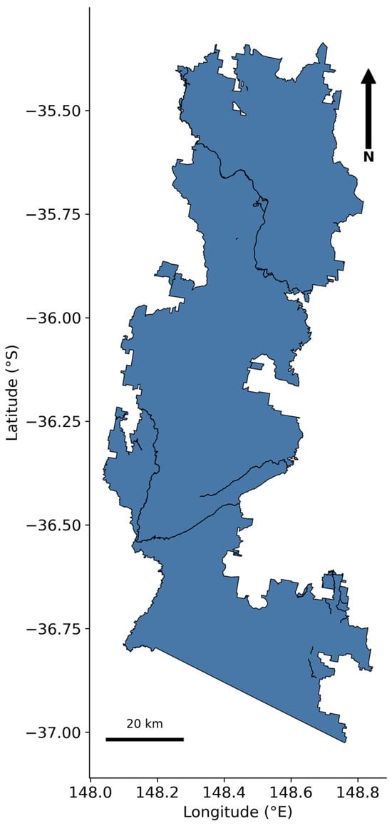
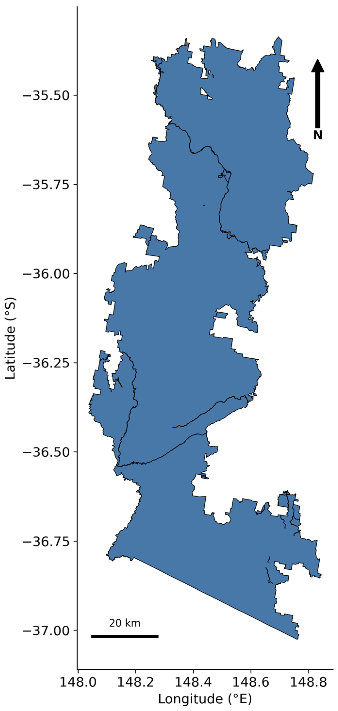
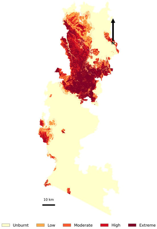
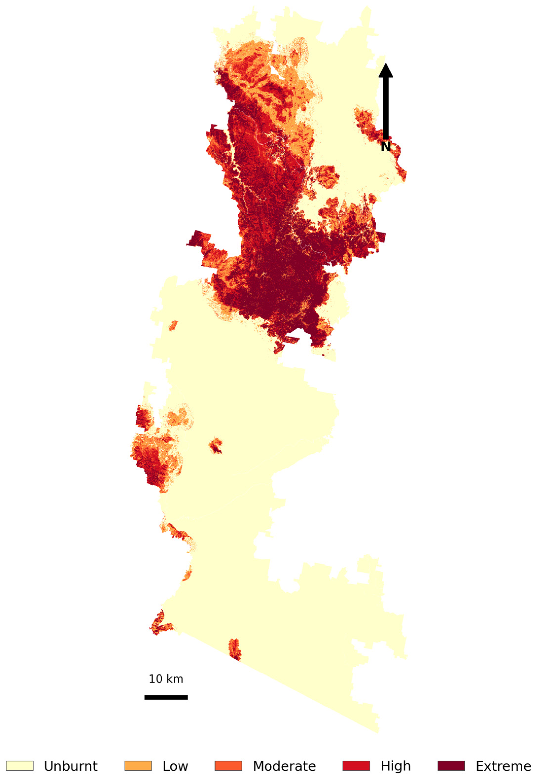
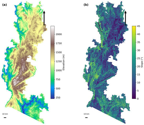
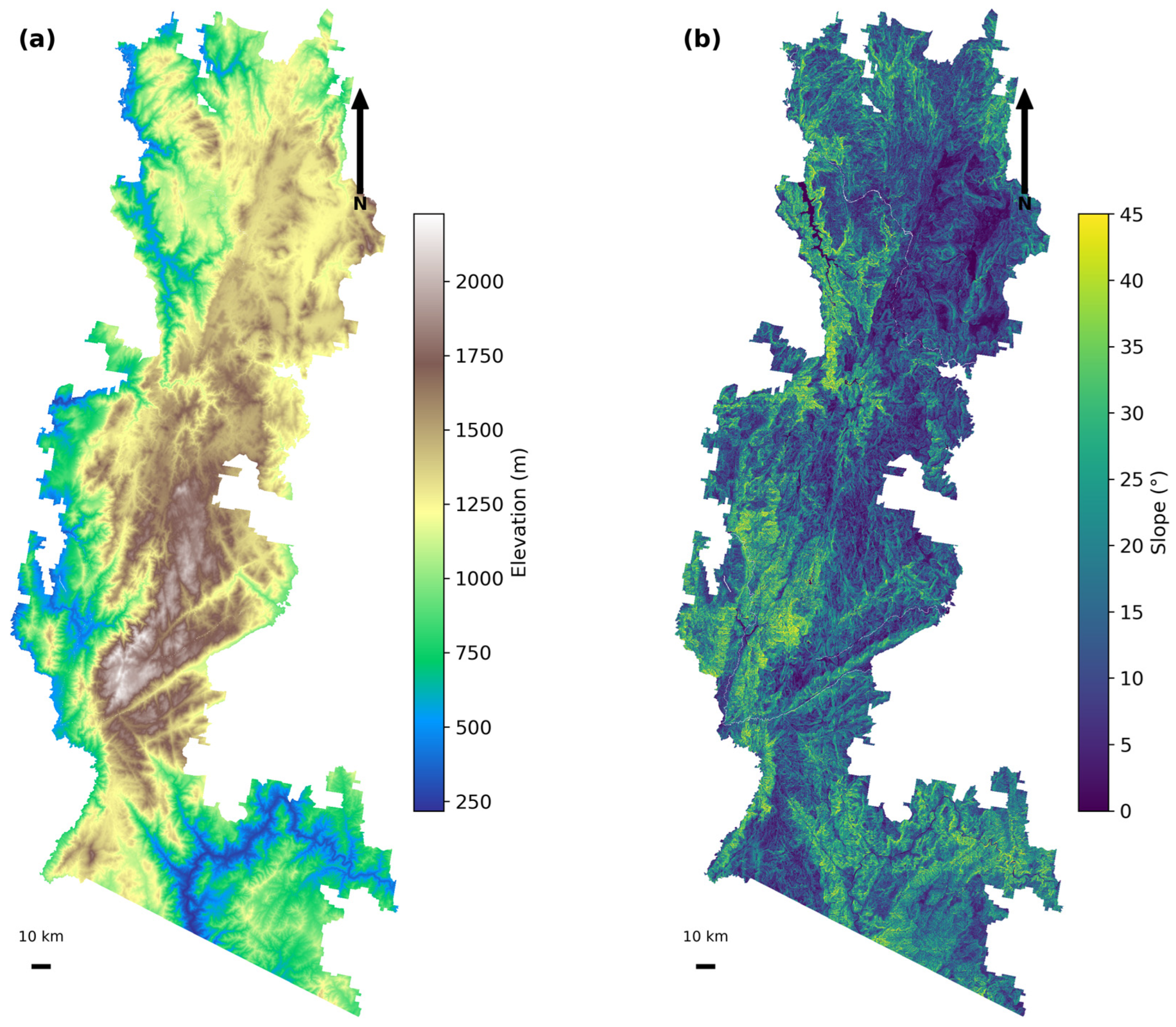
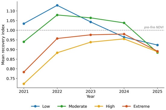
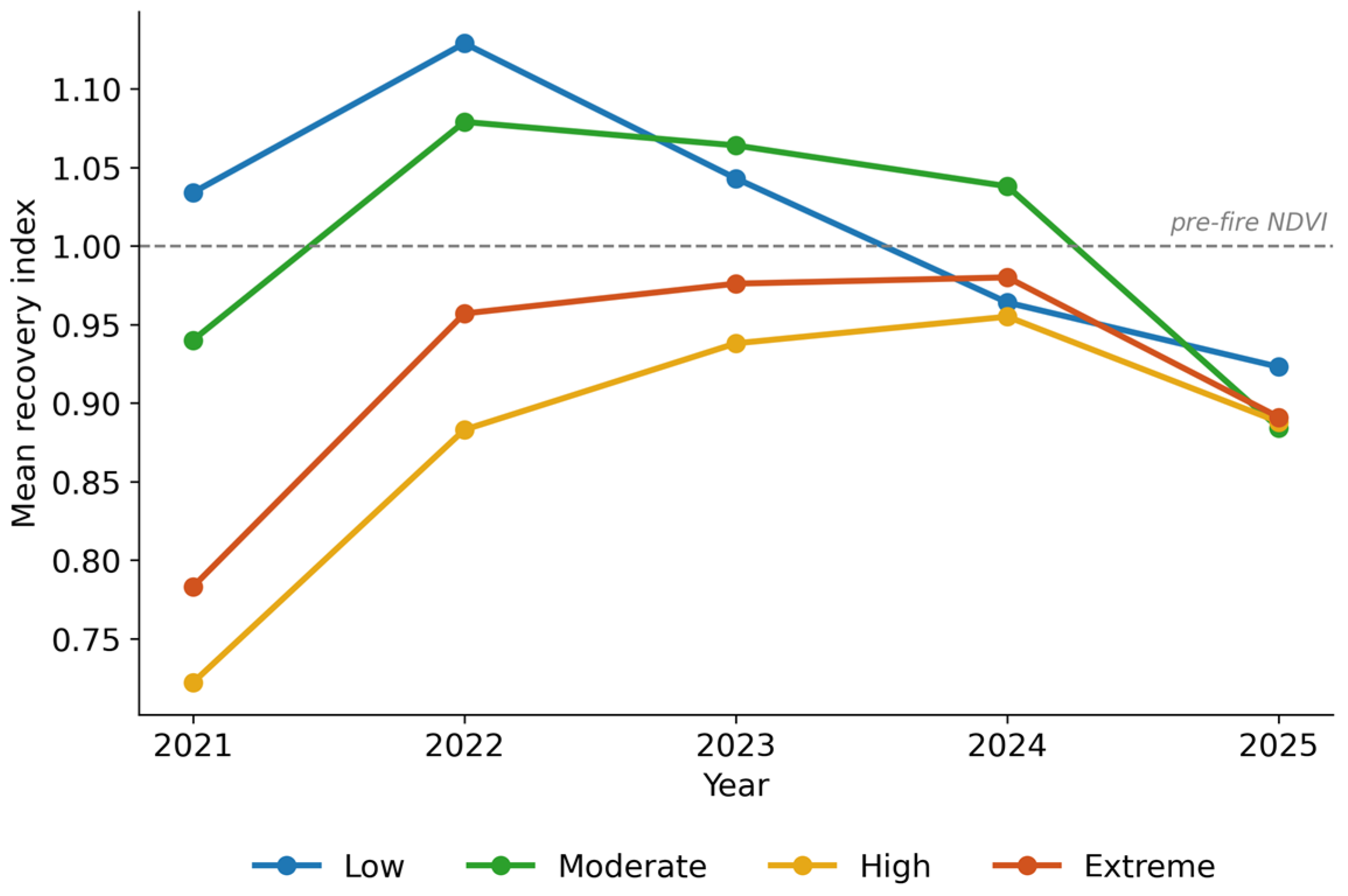
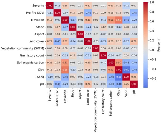
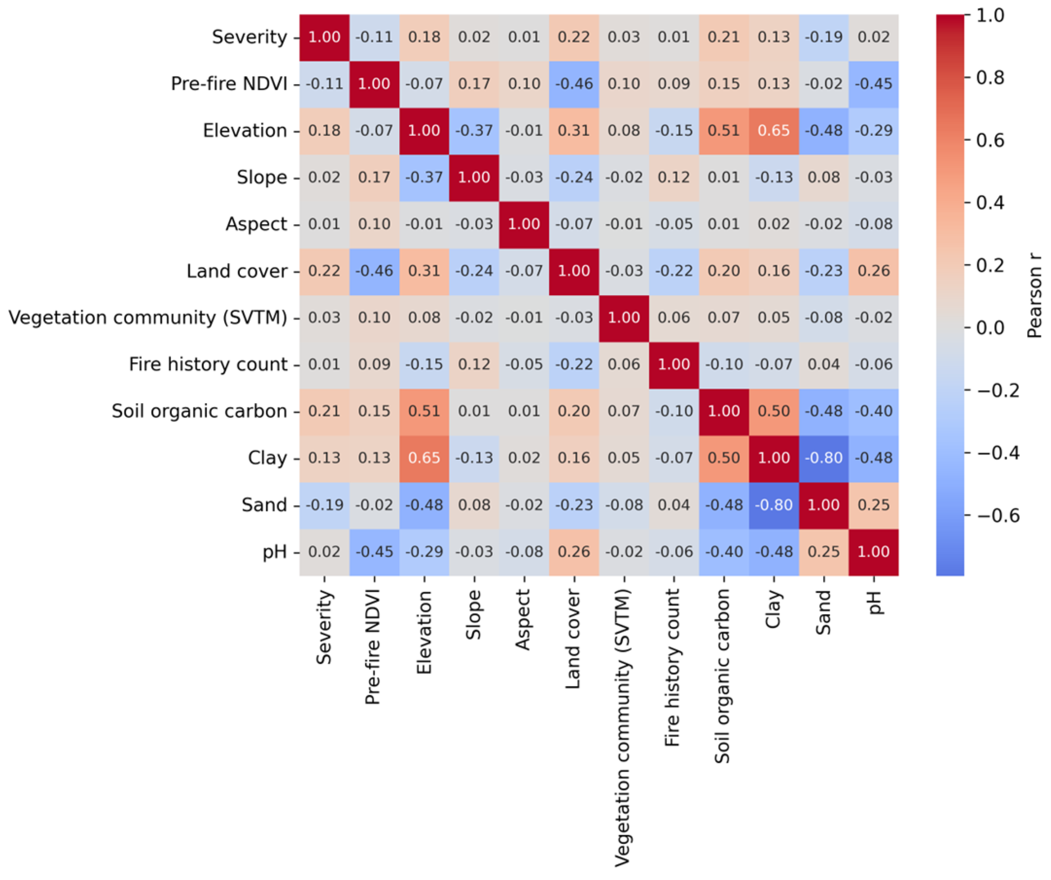
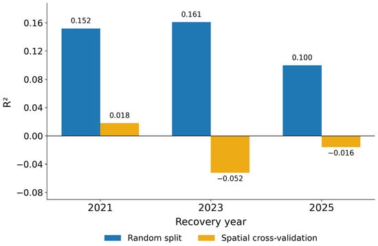
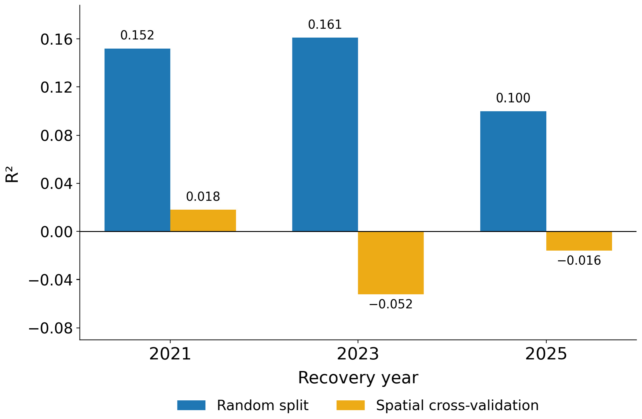
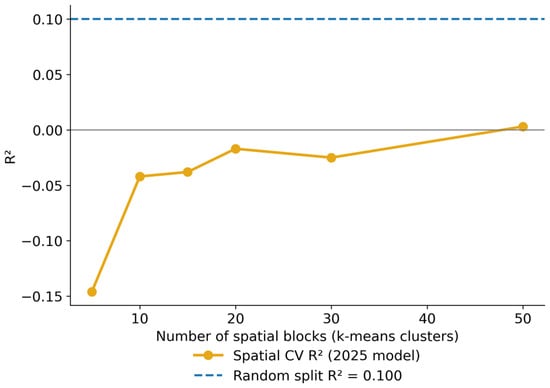
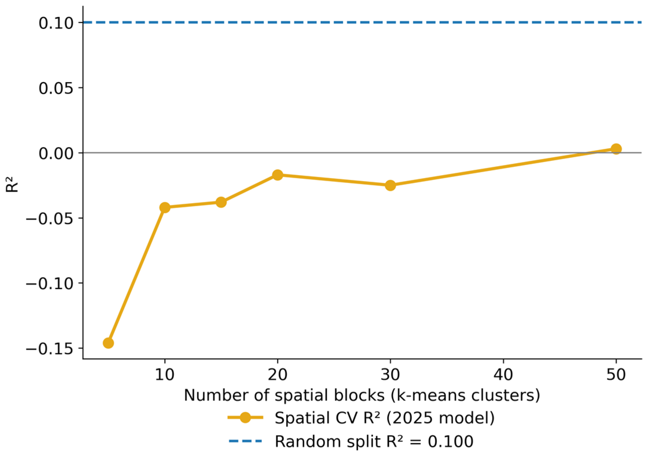
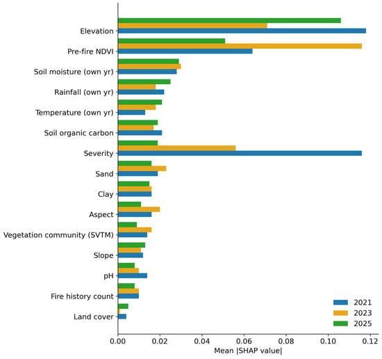
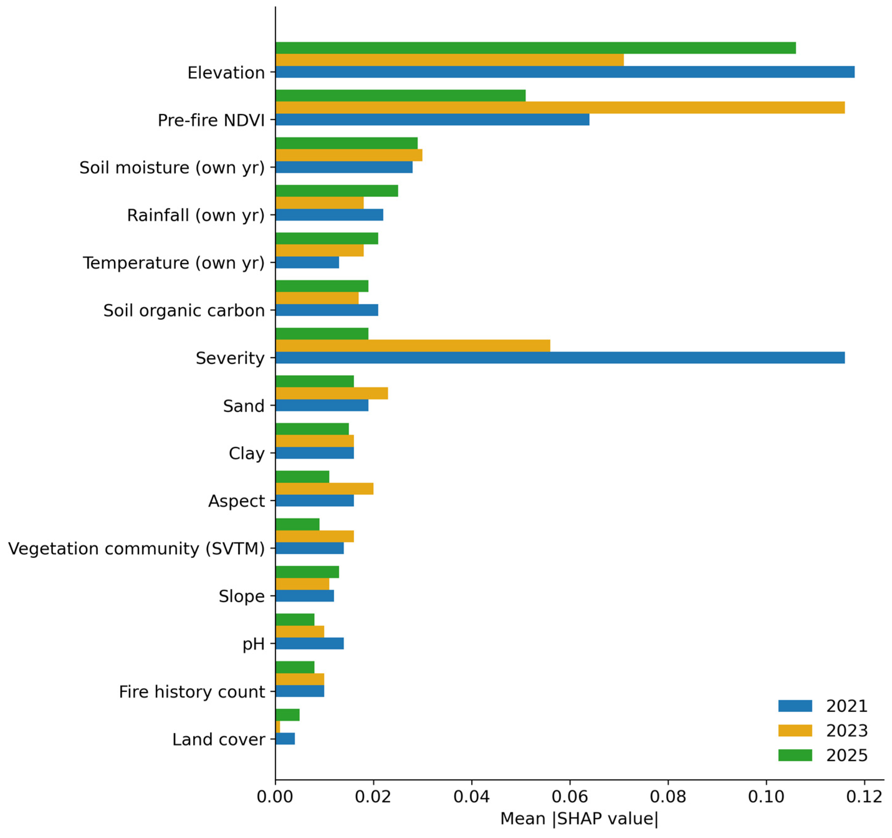
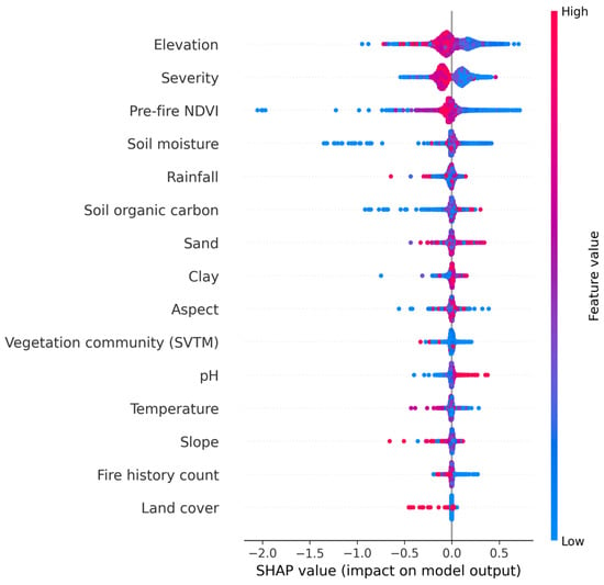
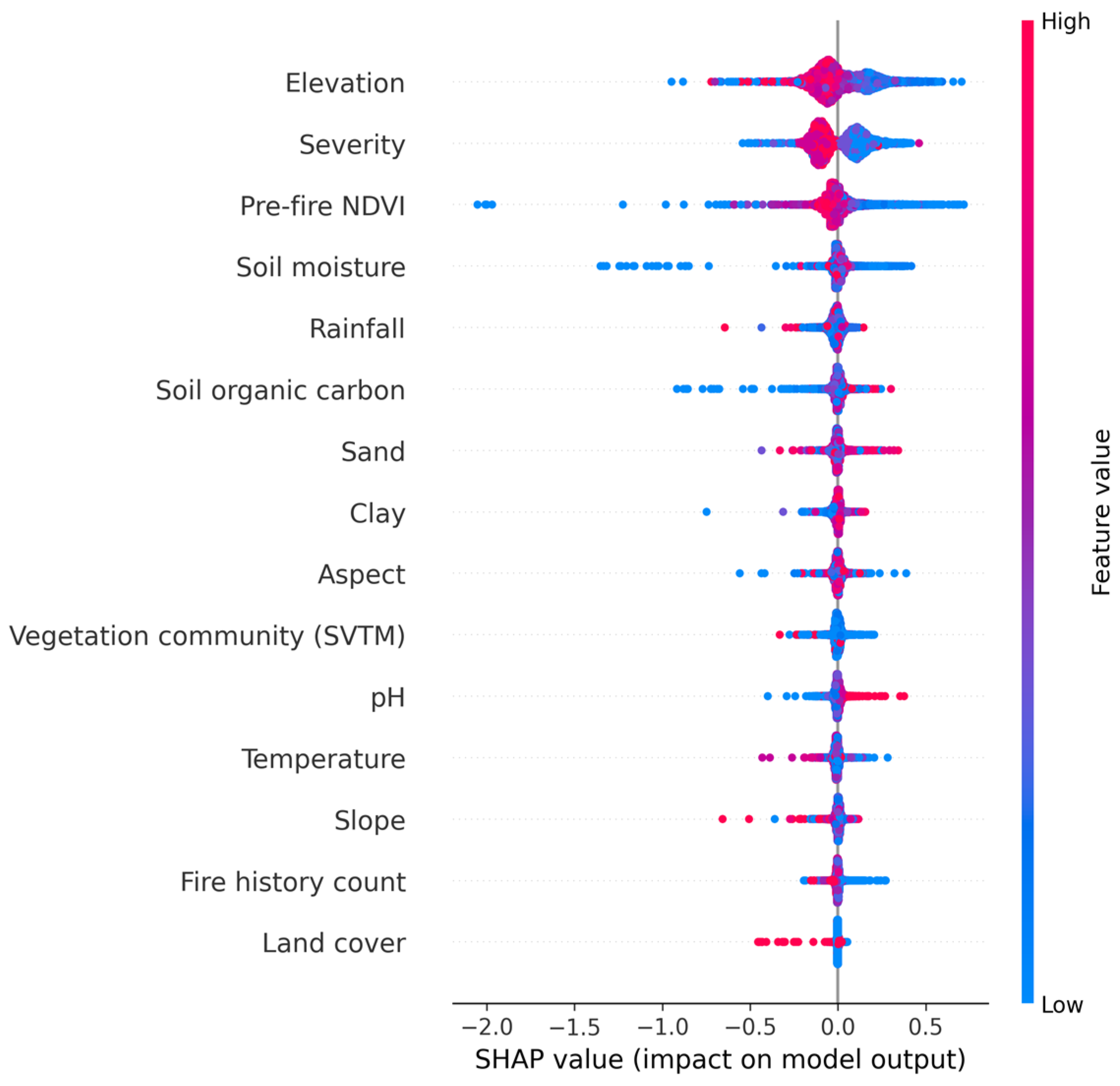
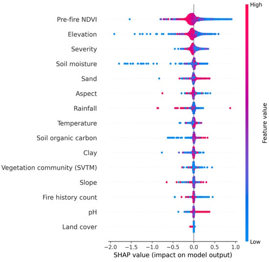
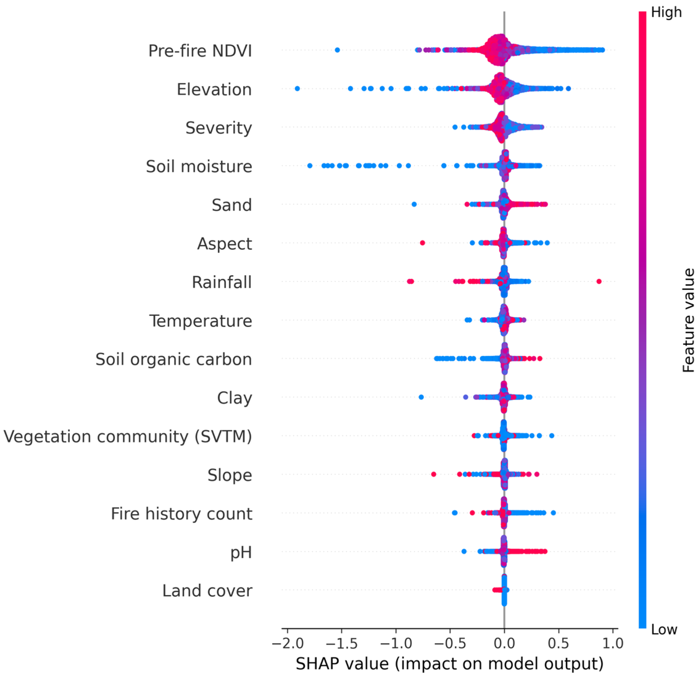
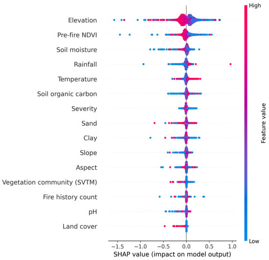
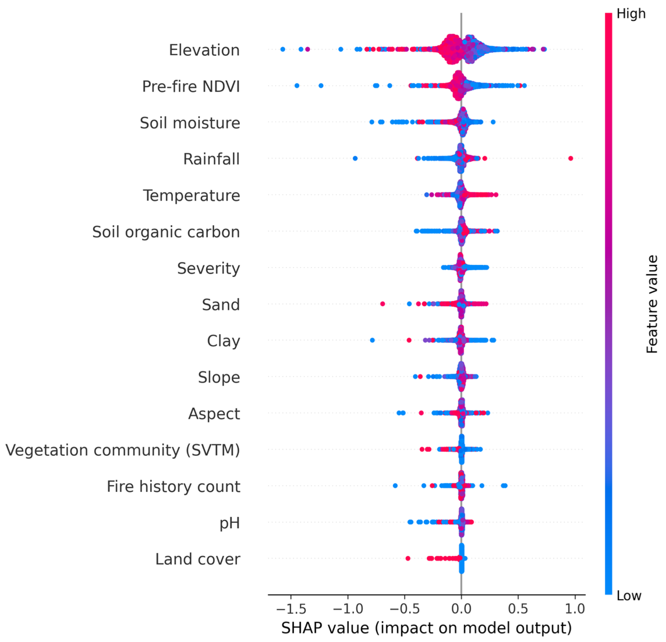
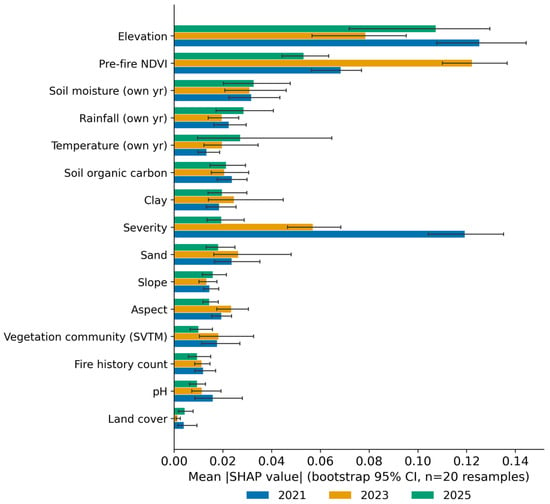
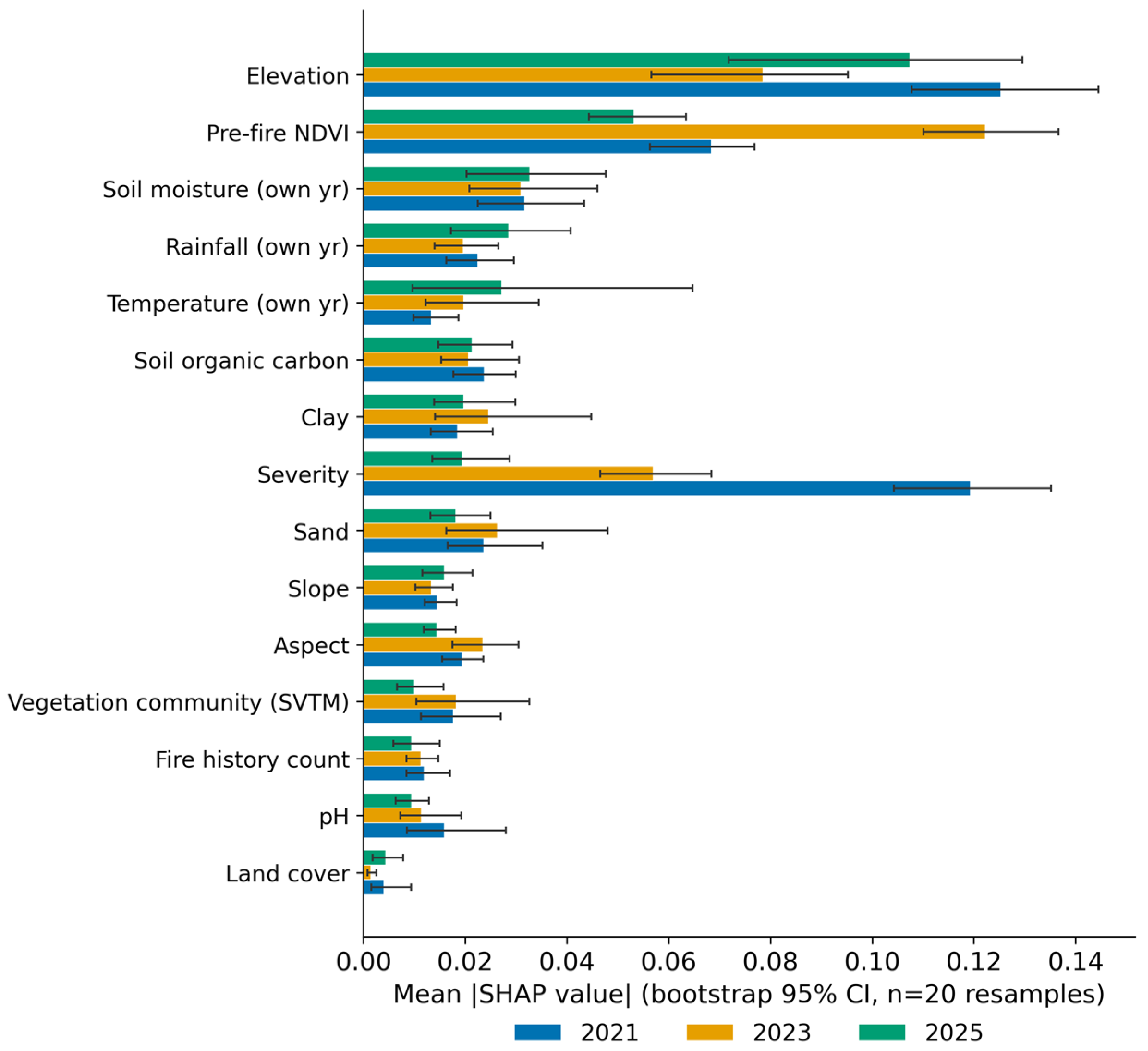
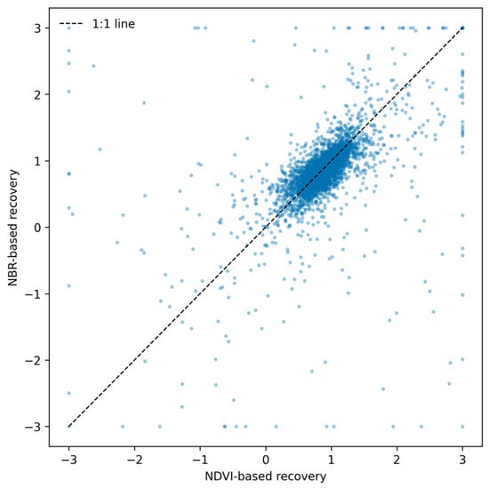
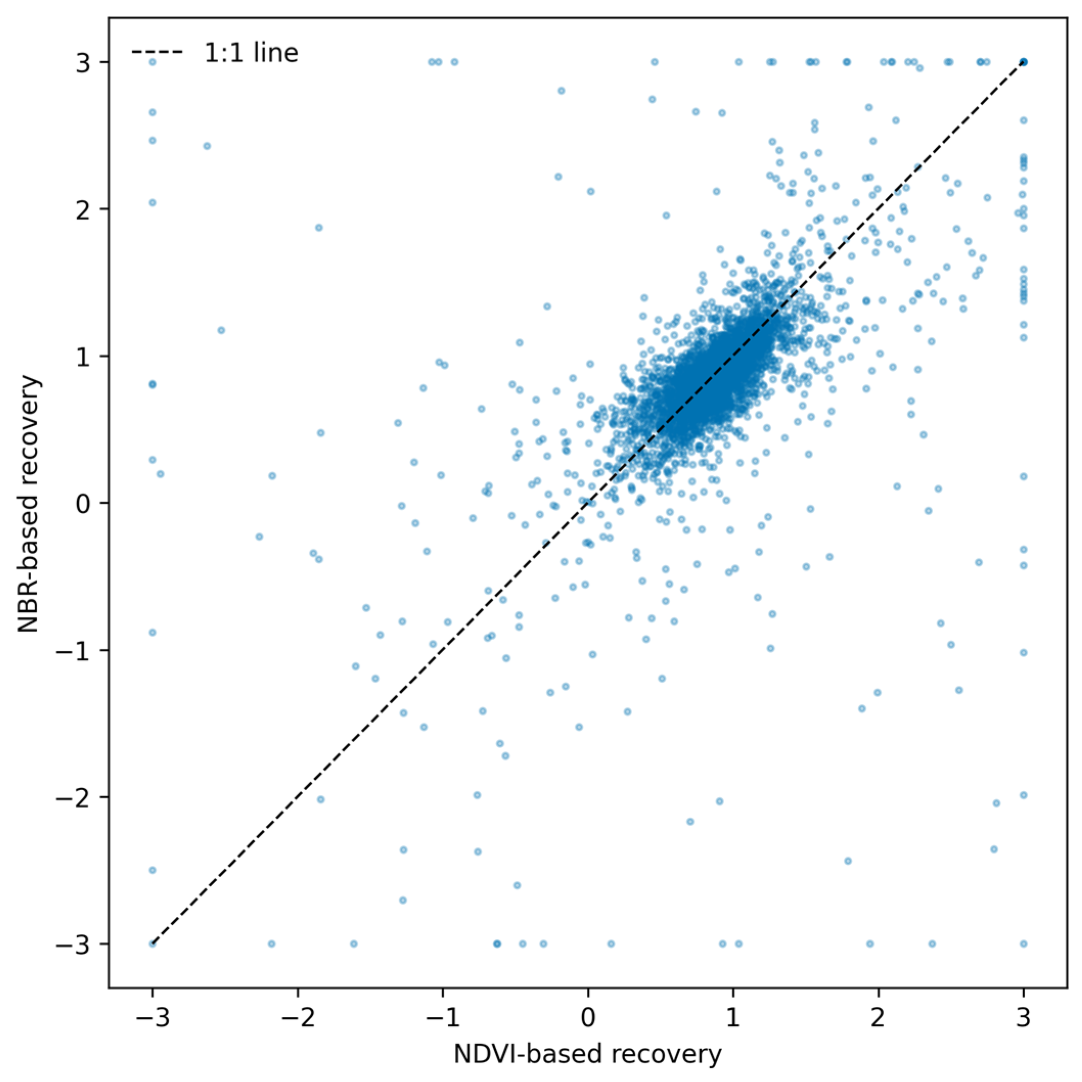
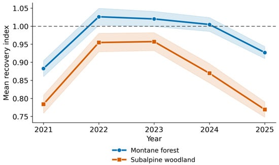
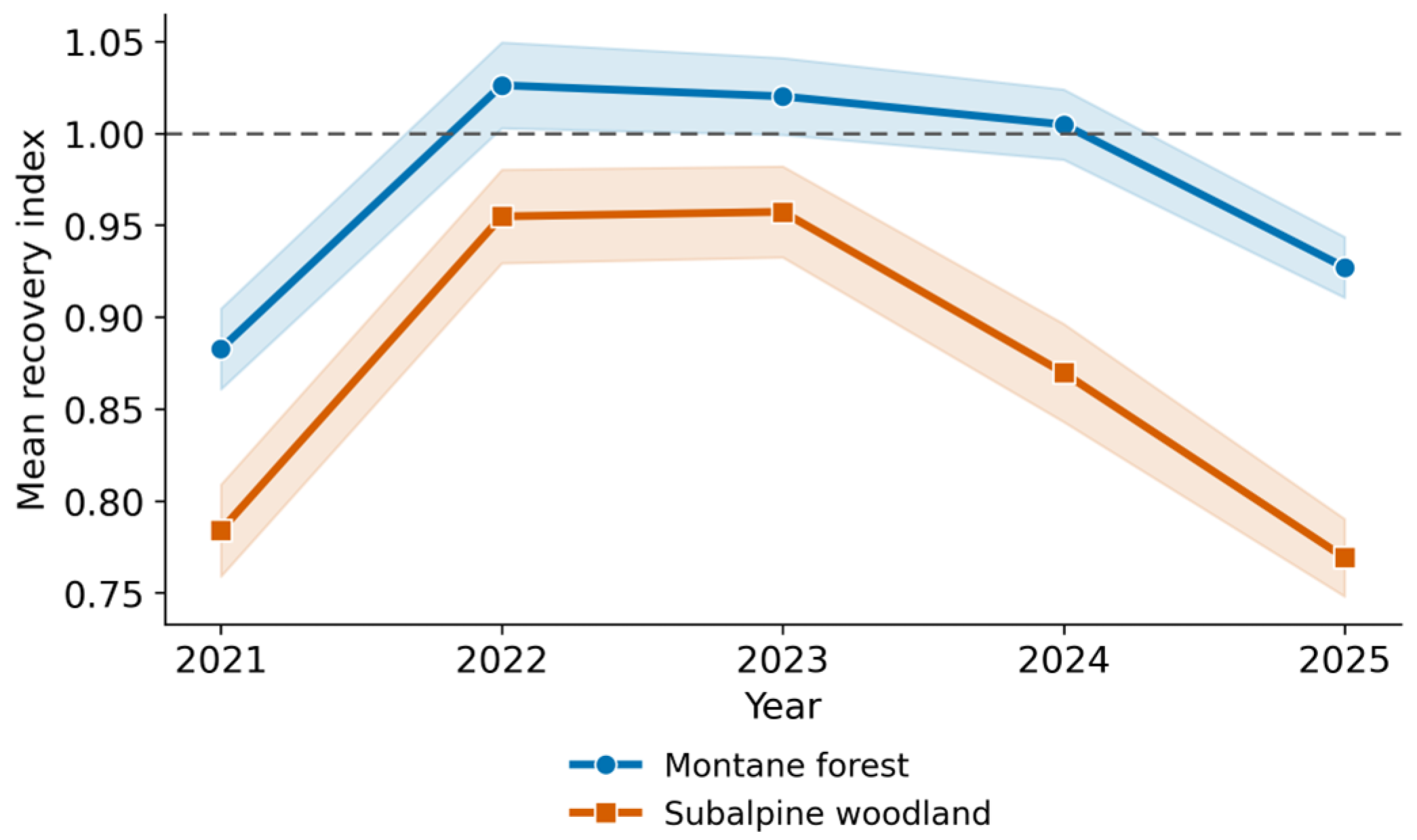
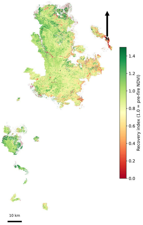
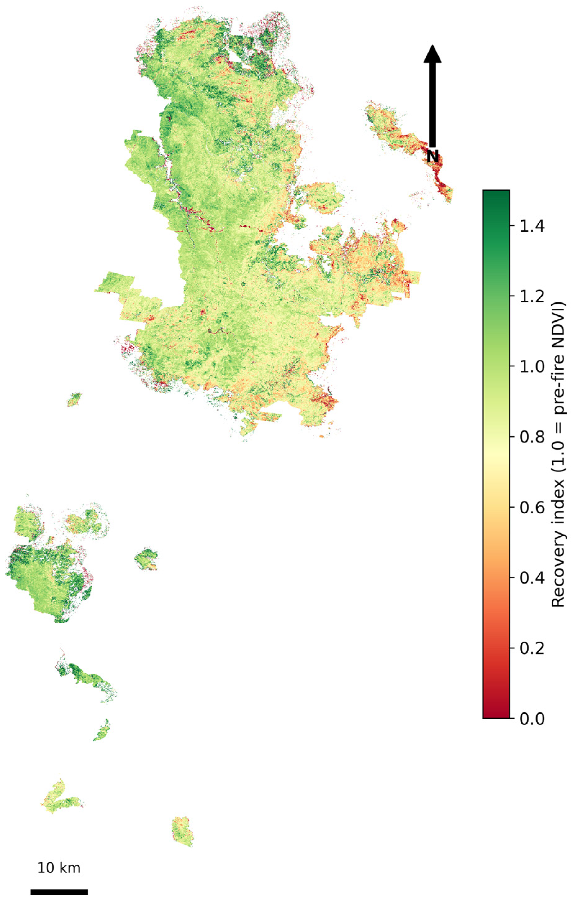
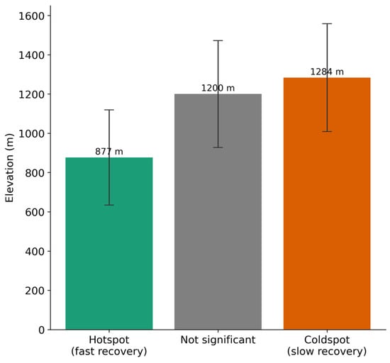
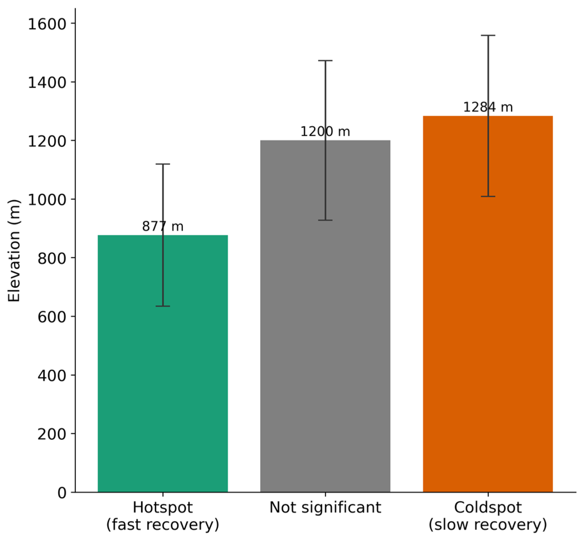
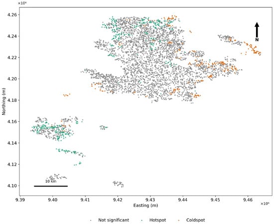
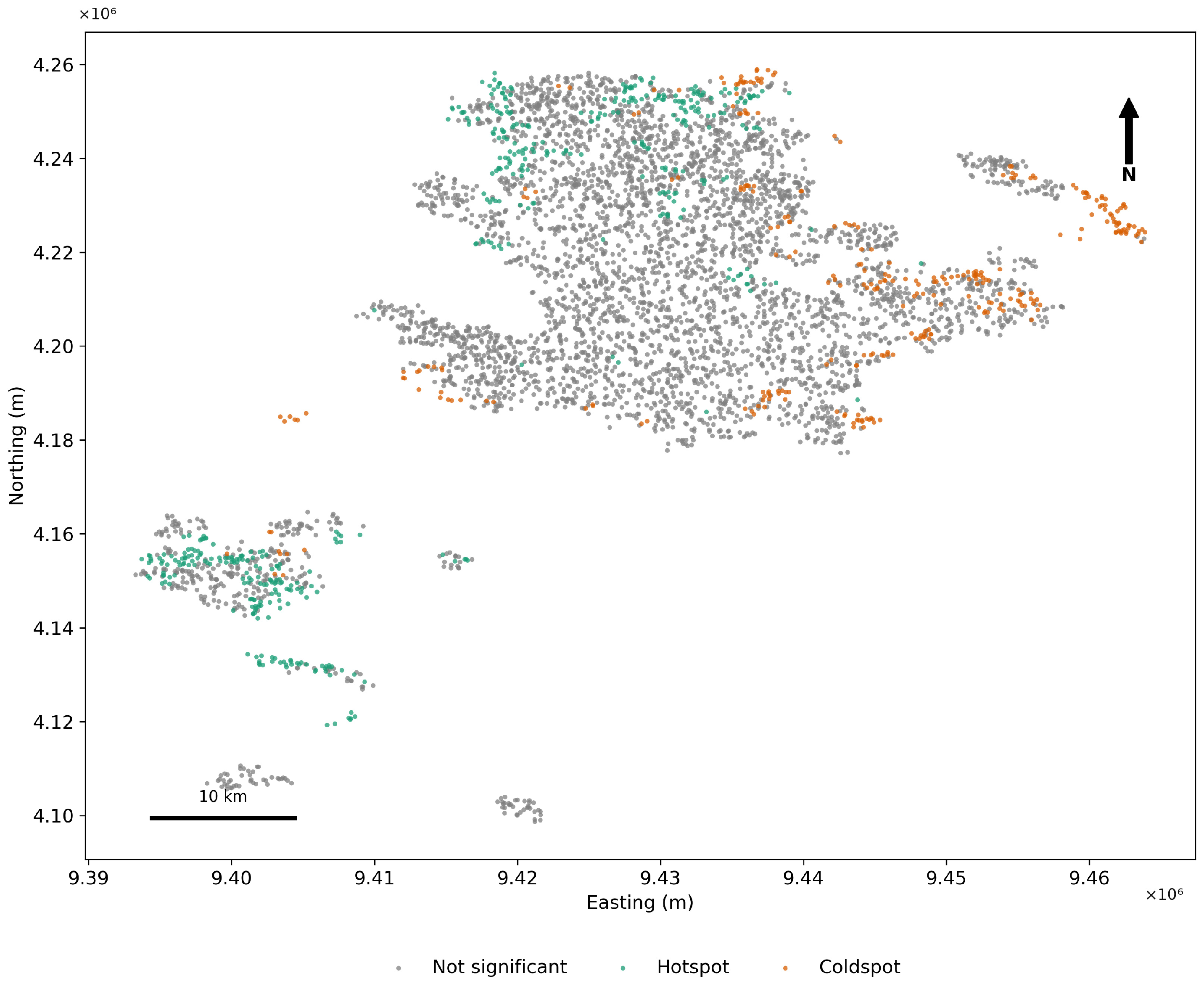
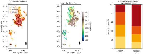
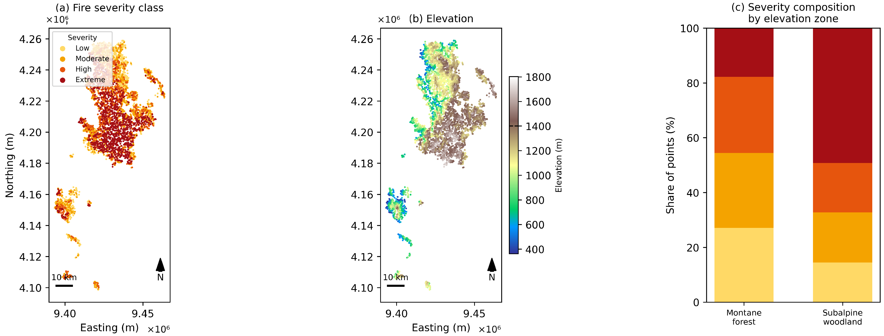

Disclaimer/Publisher’s Note: The statements, opinions and data contained in all publications are solely those of the individual author(s) and contributor(s) and not of MDPI and/or the editor(s). MDPI and/or the editor(s) disclaim responsibility for any injury to people or property resulting from any ideas, methods, instructions or products referred to in the content. |
© 2026 by the authors. Licensee MDPI, Basel, Switzerland. This article is an open access article distributed under the terms and conditions of the Creative Commons Attribution (CC BY) license.