


Abstract
Fixed-view forest smoke monitoring must distinguish weak smoke from recurrent interference under irregular observation intervals. We propose a candidate-verification framework in which the CITE-R stage combines physical-time multiscale transition representation (PMTR) with hard-negative signed residual calibration (HSRC). Contextual presence estimates anchor bounded candidate-specific corrections learned with group-level supervision. Models and thresholds are selected on non-FIgLib development data and frozen for FIgLib evaluation. Across 127 events and 27.8506 negative camera-hours, CITE-R reduces false-alarm episodes from 16 to 8 relative to the contextual presence baseline, while Recall@300 s decreases from 44.88% to 40.16%. Seed-44 validation controls yield 13/28 positive-group hits with the full design versus 2/28 for suppress-only and time-ablated variants at one false group. Matched three-seed retraining gives lower mean external recall for the full design at the primary calibration budget but higher mean recall and false-alarm rate (FAR) than both time controls at a less restrictive budget. Ten HSRC initializations with PMTR fixed reduce FAR relative to the presence baseline, with variable recall costs. The complete pipeline averages 70.62 ms per target window on an RTX 4090. Physical-time evidence and bounded signed correction provide candidate-specific control of the sensitivity–false-alarm trade-off.
1. Introduction
Visible-light cameras can monitor large outdoor areas and localize the first visible signs of forest fires. Incipient smoke is difficult to recognize because it often occupies a small, low-contrast region with diffuse boundaries. Reviews of visual smoke and fire detection identify target scale, atmospheric interference, and background complexity as persistent challenges [1,2,3].
A warning system must distinguish a useful detection from a recurrent nuisance alarm. Clouds, fog, haze, and illumination changes can resemble smoke, yet suppressing uncertain responses can also remove genuine incipient smoke. Studies using realistic smoke and non-smoke imagery [4,5] and operational camera observations [6] highlight the importance of this sensitivity–alarm-burden trade-off in deployment. Candidate verification should therefore use contextual evidence to strengthen supported smoke responses and suppress persistent interference.
Publicly available resources support more detailed investigations of this problem. FIgLib and SmokeyNet provide fixed-view spatio-temporal data and modeling [7]; Nemo emphasizes fine-grained and incipient smoke [8]; and PYRONEAR-2025 includes image and sequential observations from multiple sources [9]. Lightweight spatio-temporal detectors also exploit information beyond individual images [10]. For camera-based warning, however, these representations must be evaluated in terms of event sensitivity and repeated false-alarm episodes because image-level discrimination alone does not determine alarm workload.
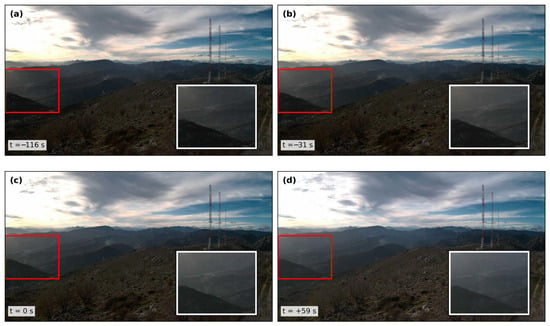
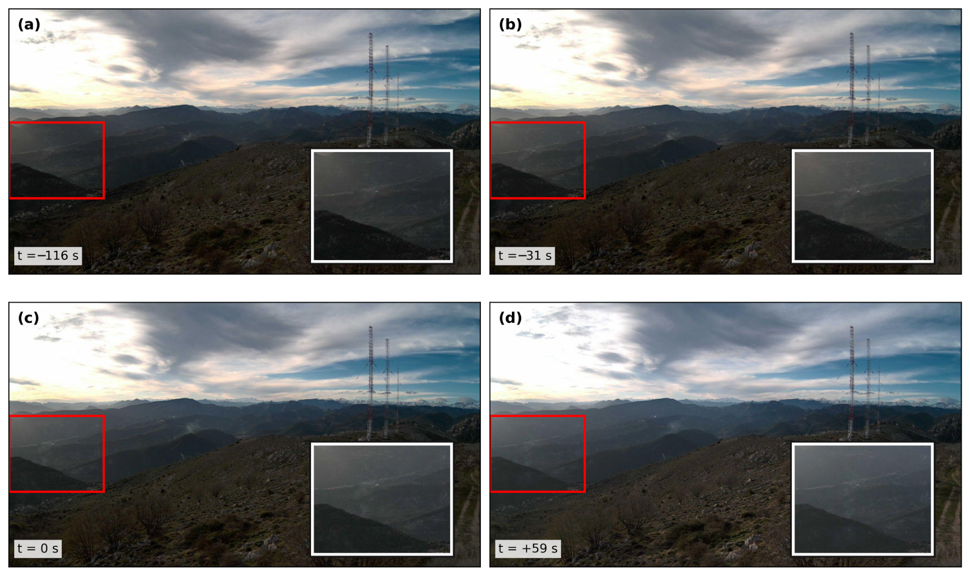
Figure 1 illustrates the task using a real PyroNear2025-V sequence [9]. A small region on a distant hillside must be interpreted against terrain and extensive cloud cover. Unequal observation intervals further complicate comparisons between adjacent frames. This setting motivates both a scene reference that preserves emerging candidates and a verification mechanism that uses actual elapsed time.
Figure 1.
Fixed-view forest observations from PyroNear2025-V [9]. Panels (a–d) show the same region at −116, −31, 0, and +59 s relative to the first positive annotation. The −31 s observation is the protocol-suggested boundary for this example. Red rectangles indicate the region used to illustrate weak visibility and irregular sampling; the white-bordered insets show enlarged views of the regions marked by the red rectangles.
This study addresses three connected decisions: how to adapt a reference without rapidly absorbing a suspicious region, how to interpret a candidate relative to its neighborhood and the wider scene, and how to use irregularly spaced history to revise its current score. The last decision is central. Historical evidence can support smoke detection as well as reject interference, so the temporal update should permit both positive and negative corrections.
The framework retains a frozen candidate detector. Time-aware dual-timescale normality adaptation (TDNRI) constructs protected reference states and residual features. A candidate–context evidence head (CCEH) combines local appearance, neighborhood context, reference residuals, and global scene information into a smoke-presence logit. CITE-R then applies a physical-time multiscale transition representation (PMTR) and hard-negative signed residual calibration (HSRC) to this logit. The final update is candidate-dependent and bounded; calibration refers to alarm-oriented score adjustment rather than probability calibration.
The main contribution is a candidate-specific, bounded signed correction that combines physical-time transition evidence with group-level alarm supervision. It allows weak smoke responses to be strengthened while learning to suppress high-scoring nuisance groups. Protected reference adaptation and local–neighborhood–scene relations provide the contextual presence anchor. Controlled comparisons and source-out event evaluation link this design to recall and false-alarm burden.
The frozen-threshold FIgLib comparison measures the transferred recall–false-alarm trade-off: CITE-R halves false-alarm episodes while detecting six fewer of 127 events within 300 s. The mechanism controls examine the contributions of physical-time information and positive residual correction to this verification design.
1.1. Visual Smoke Detection and Candidate Verification
Earlier video smoke detectors combined wavelet features with support vector machines [11] or used spatial context alongside motion, color, texture, and shape [12]. These approaches established the value of interpreting a suspected smoke region together with its surroundings. Learned verification extends this principle by combining candidate appearance with contextual and temporal evidence.
Visual fire and smoke detection methods address weak targets through multiscale representation, attention, and localization [1,2,3]. Peng and Wang combined candidate extraction with a compact classifier [13], while DeepSmoke coupled recognition and segmentation for outdoor environments [14]. Zheng et al. compared mainstream detectors for forest smoke localization [15]. MVMNet [16], BCMNet [17], and SMWE-GFPNNet [18] developed specialized attention, cross-layer interaction, and smoke-oriented feature fusion. These methods improve the visual evidence available for candidate decisions.
Efficient architectures such as RT-DETR [19] also provide candidate generators for verification pipelines. Jung et al. combined multi-resolution inputs with selective second-stage classification [20]. Other work addresses ambiguous positive regions and hard-negative backgrounds through data and training design [21] or targets recognition with very low false-positive rates using EfficientNets [22]. PSNet [23] and LMINet [24] further investigate representations that distinguish smoke from interference.
STV-FSANet groups detections into tracks and combines appearance and geometry to verify fire, smoke, and false-alarm tracks [25]. CITE-R organizes verification around a reference at the current candidate location, explicit candidate–scene relations, and a physical-time-conditioned correction to the presence logit. The resulting bounded update links contextual recognition to the alarm decision.
1.2. Temporal Evidence and Time-Aware Decision Correction
Temporal smoke recognition has used bidirectional recurrent modeling and attention [26], foreground-enhanced features [27], adaptive frame selection [28], and temporal relations that reduce spatial and semantic interference [29]. SmokeyNet [7], the PYRONEAR-2025 sequential benchmark [9], and LwST-FSD [10] demonstrate the relevance of historical information for fixed-view monitoring. Krstinić et al. encode short- and long-term temporal and contextual information as additional image channels for YOLO architectures [30].
Operational studies also integrate complementary evidence. Bhamra et al. proposed Multimodal SmokeyNet, which integrates camera imagery with weather measurements, and SmokeyNet Ensemble, which combines camera-based, satellite-based, and weather-based predictions [31]. EARL learns normal scene dynamics and uses emergence cues with a training objective that accounts for detection delay and false alarms [32]. Together, these studies connect smoke recognition to nuisance rejection and warning time. CITE-R pursues this objective through RGB-derived candidate evidence, actual observation intervals, and a signed correction to an existing presence estimate.
Elapsed-time modeling is also established in general sequence learning: GRU-D incorporates observation masks and time intervals [33]. Here, elapsed time serves three task-specific roles. It regulates protected reference adaptation, defines the retrieval horizons for candidate transitions, and conditions a bounded signed update learned with group-level alarm supervision.
This design separates temporal representation from the final decision objective. PMTR encodes observed changes; HSRC uses the frozen encoding to adjust the CCEH presence anchor. Group-balanced classification, hard-negative ranking, and candidate-level supervision train that adjustment at complementary levels. The experiments consequently examine the physical-time representation and signed correction separately before interpreting their combined alarm behavior.
2. Materials and Methods
2.1. Data Roles and Supervision
The experiments separate static detector development, temporal-model development, reviewed visibility-boundary analysis, and FIgLib source-out evaluation. Table 1 summarizes the inputs and supervision used at each stage. Supplementary Materials Sections S2 and S7 give the archive inventories and source mappings.
Table 1.
Data roles and archived experimental populations. Counts refer to the image lists, window protocols, supervised candidate records, or reviewed events used at the indicated stage.
Detector development begins with cleaned Pyro-SDIS images obtained from the official PyroNear dataset repository [34] and continues on the retained non-FIgLib PyroNear2025-I lists. The temporal development caches use non-FIgLib training and validation data; all FIgLib entries in the audited feature cache have the external-test role. Supplementary Materials Sections S2 and S7.6 report archive totals, annotation availability, source mappings, and protocol overlap checks.
The reviewed onset set contains 46 training and 29 validation events, each with a last confirmed no-smoke observation L and a first confirmed visible-smoke observation R. Endpoint reconstruction produces 288 windows across these 75 events. No observed frame lies strictly inside an L–R interval; R is therefore an observed visibility boundary, not a reconstructed continuous-time onset. The reviewed negative set contains 292 training and 37 validation units.
CCEH uses 58,746 training and 13,738 validation candidates with positive or negative supervision. When valid positive geometry is available, a maximum IoU of at least 0.30 defines a positive candidate and an IoU of at most 0.05 defines a negative; intermediate overlaps are ignored. Valid empty-label frames provide negative candidates, while missing labels and invalid positive geometry are excluded. The frame-level TDNRI protection mask is constructed separately. Complete label-state and candidate counts are provided in Supplementary Materials Tables S14 and S18.
FIgLib contributes 127 reviewed positive events for source-out recall [7]. The negative evaluation uses 22 reviewed no-smoke streams, comprising 1646 windows and 27.8506 database-covered camera-hours. Checkpoints and thresholds are selected on non-FIgLib development data and frozen before evaluation. Review decisions and stream exclusions are documented in Supplementary Materials Section S7.
2.2. Candidate-Anchored Verification Framework
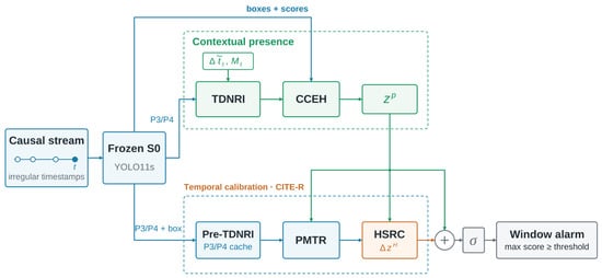
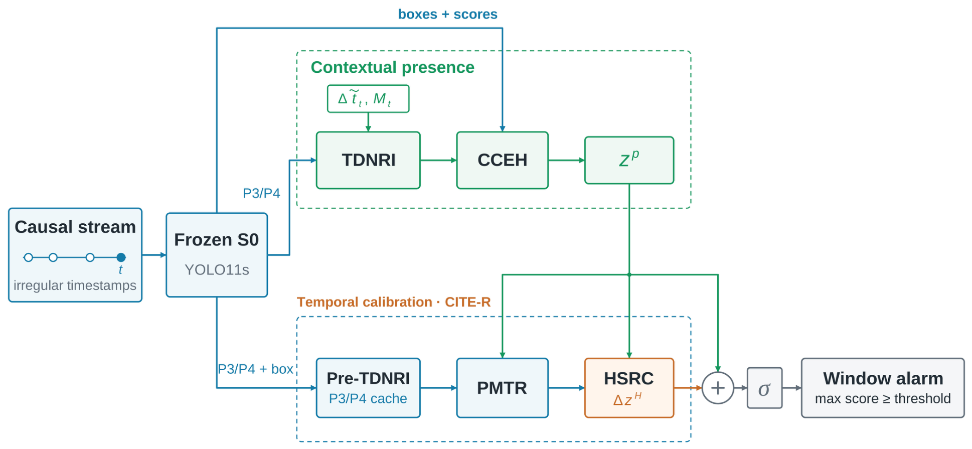
For an RGB image observed at time t, the frozen YOLO11s-based detector S0 [35] produces candidate boxes, confidence scores, and intermediate features. Verification rescores these candidates without creating an independent detection set. Figure 2 shows the contextual presence path and the temporal correction path.
Figure 2.
Candidate-anchored verification framework. TDNRI and CCEH produce the contextual presence estimate. PMTR uses pre-TDNRI detector features to represent physical-time transitions. HSRC combines the PMTR outputs with the original presence logit and adds the final bounded signed residual. Arrows indicate the direction of information flow. Blue represents detector data and temporal features, green represents the contextual presence pathway, orange represents the final signed residual, and gray represents the alarm decision pathway.
TDNRI and CCEH construct the current presence estimate from reference-relative and scene-relative evidence. In parallel, PMTR retrieves pre-TDNRI detector features at the current candidate location to describe historical changes. The first path estimates presence; the second provides evidence for revising that estimate. CITE-R denotes the PMTR–HSRC correction stage applied to the CCEH anchor.
Denoting the original CCEH presence logit by the superscript pres and the final HSRC correction as Δzᴴ, the candidate-level output is
where σ is the sigmoid function. Positive residuals can raise supported candidates above the alarm threshold, while negative residuals can suppress nuisance responses. Historical inputs are strictly earlier than the current timestamp. Because the correction operates on S0 proposals, its output remains constrained by their availability and quality.
S0 uses a 1024-pixel input, a candidate confidence threshold of 0.01, an NMS IoU threshold of 0.70, and at most 20 detections per frame. Adaptive pooling of layer-16 and layer-19 activations produces P3-derived and P4-derived tensors of 128 × 16 × 16 and 256 × 8 × 8. Both paths use the same detector tensors but construct different downstream representations. Supplementary Materials Section S1 gives the implementation details.
2.3. Candidate-Protected Reference Adaptation
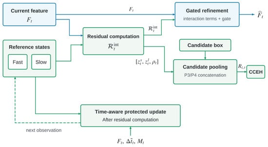
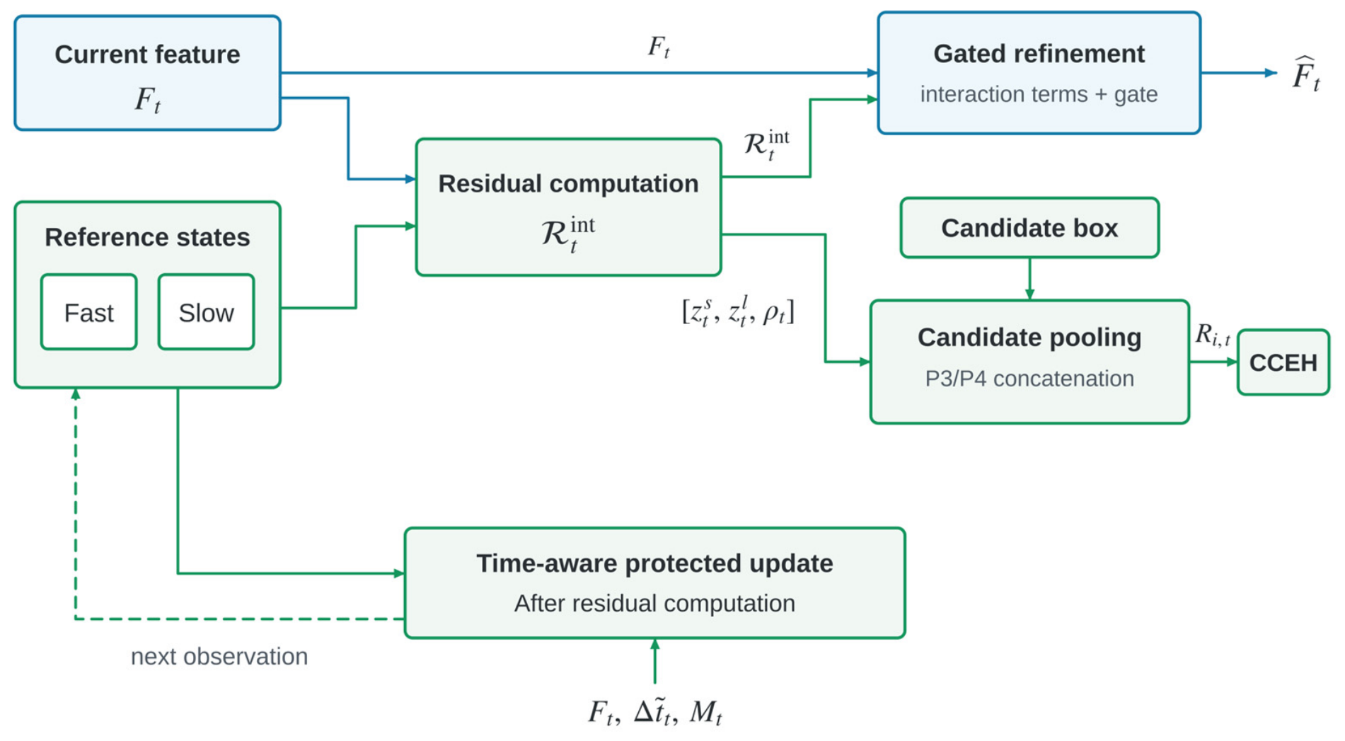
A fixed viewpoint provides a reference for interpreting change, but rapid adaptation can absorb emerging smoke. TDNRI couples elapsed-time adaptation with detector-derived candidate protection. At each feature scale, it maintains fast and slow mean and variance states. The current observation is first compared with the preceding states; the states are updated only after the residuals have been computed (Figure 3).
Figure 3.
Candidate-protected reference adaptation at one feature scale. Fast and slow states provide standardized residuals and a variance-ratio cue before the current observation updates them. These cues refine detector features and form candidate descriptors. Elapsed time and the candidate mask control the subsequent update. P3 and P4 maintain independent states, which are reset for each four-observation window. Solid arrows show the direction of information flow when processing the current observation. The dashed green arrow indicates that the updated reference states are carried forward to the next observation.
In the reference update, Δtt denotes elapsed seconds divided by 30; q identifies the fast or slow state. The temporal coefficient and its spatially protected counterpart are
where Mt is the binary detector-supported-region mask resized to the feature scale. The final settings are τs= 2.5, τl = 20, and κ = 0.95, corresponding to nominal physical-time constants of 75 and 600 s. A protected location receives 5% of the ordinary update rate. Elapsed time thus determines the amount of adaptation, while the mask determines where adaptation is slowed.
For current detector features Ft, standardized residuals and the log-variance ratio are
The internal residual tensor combines short- and long-timescale deviations, their interaction, their difference, and the variance-ratio cue:
The current feature and the internal residual tensor are fused through a depthwise 3 × 3 convolution, BatchNorm, and SiLU. Learned 1 × 1 projections produce a channel gate and the residual feature update:
The learned residual scale γ is initialized to 10−3. The mean and variance states are subsequently updated using
with element-wise operations and spatial coefficients broadcast over channels. Computing residuals before this update ensures that the current score is calculated relative to the preceding state.
Each causal four-observation window initializes both means from its first feature map and both variances to 1.0. The reference is estimated from the available window history. The nominal 75 s and 600 s time constants specify adaptation rates; the actual observation span is determined by the four retained timestamps.
For CCEH, only the short residual, long residual, and log-variance ratio are pooled over each candidate. Concatenating these cues across P3 and P4 produces the 1152-dimensional residual descriptor. The interaction and difference terms remain in feature refinement but are not separately included in this descriptor.
2.4. Candidate and Scene Relations for Presence Estimation
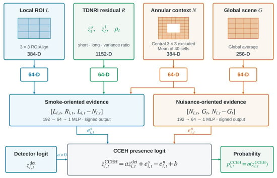
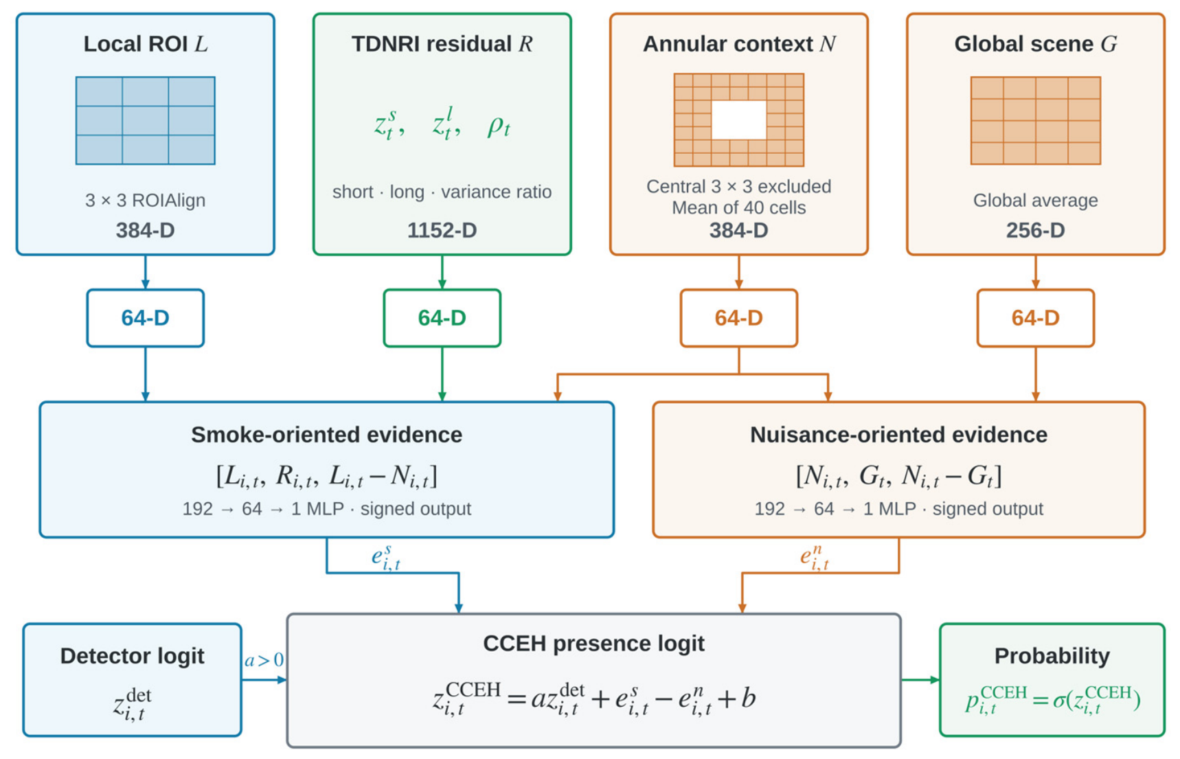
CCEH estimates presence based on a candidate’s relationships with its surroundings (Figure 4). It receives a 384-dimensional local descriptor L, a 384-dimensional annular-neighborhood descriptor N, a 256-dimensional global descriptor G, and the 1152-dimensional TDNRI residual descriptor R. Local and neighborhood descriptors use the refined P3/P4 maps; G is the spatial average of refined P4.
Figure 4.
Relation-based presence estimation with CCEH. Four descriptors are independently projected to 64 dimensions. The local branch combines appearance, reference residuals, and local–neighborhood contrast; the scene branch combines neighborhood, global context, and neighborhood–global contrast. Their signed outputs modify a positively scaled detector logit. The smoke-oriented and nuisance-oriented labels describe input roles, not fixed output signs. Arrows indicate the flow of features and scores. Blue marks the local appearance input and the smoke-oriented branch, green marks the TDNRI residual input and the output probability, and orange marks the neighborhood and global inputs and the nuisance-oriented branch.
Local pooling uses 3 × 3 ROIAlign over the candidate box. Neighborhood pooling expands the box by a factor of 1.75, applies 7 × 7 ROIAlign, and averages the 40 cells outside the central 3 × 3 region. The term annular neighborhood refers to this central-cell exclusion on the pooled grid, not an exact geometric mask of the original candidate box. The same grid rule is applied after clipping at the image boundary. Supplementary Materials Section S1.1 specifies the construction.
Each descriptor is independently projected to 64 dimensions by a linear layer, LayerNorm, and SiLU. The two branches then encode local–neighborhood and neighborhood–global relations:
Each branch is a 192 → 64 → 1 MLP with LayerNorm, SiLU, and hidden-layer dropout. The original detector confidence is clipped and converted to a logit. CCEH combines it with the branch outputs as
followed by a sigmoid. The positive coefficient retains a direct detector-evidence path, and both relation branches provide unconstrained signed adjustments. Consequently, subtracting the neighborhood–global output does not necessarily reduce the final logit. The final C5 configuration uses no nonzero auxiliary competition loss.
2.5. Physical-Time Multiscale Transition Representation
PMTR describes changes at the current candidate location over actual elapsed time. It uses cached S0 features before TDNRI refinement. For both current and historical observations, 3 × 3 ROIAlign features at the current box are spatially averaged on P3 and P4 and concatenated into a 384-dimensional regional vector. Each vector is L2-normalized.
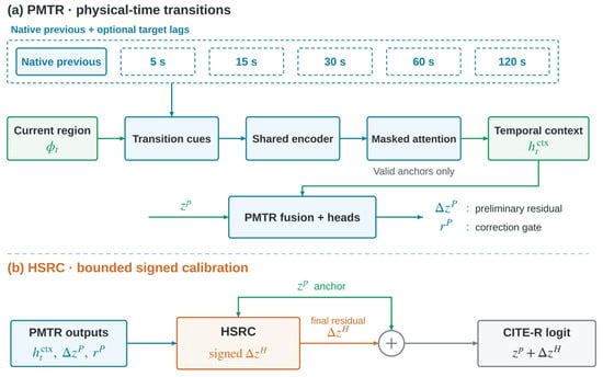
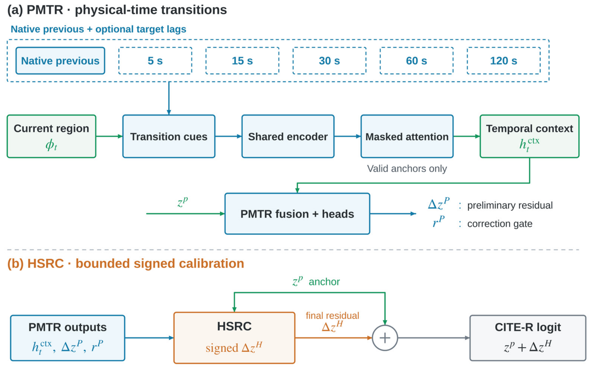
Every sample entering the evaluated PMTR path retains one native preceding observation. Optional historical observations are retrieved at around 5, 15, 30, 60, and 120 s. For each target lag, the nearest causal observation is accepted when its lag error is at most max(3 s, half the target lag). A frame assigned to one physical-time slot is not reused in another; unavailable slots are masked. Figure 5 summarizes this retrieval and its connection to the final correction. Supplementary Materials Section S1.1 gives the implementation details.
Figure 5.
Physical-time representation and signed correction. PMTR encodes the native preceding observation and optional elapsed-time anchors, then produces temporal context, a preliminary residual, and a correction gate. HSRC uses these outputs and the original presence logit to predict the final residual. Hard-negative ranking is used during training. Arrows indicate the direction of information flow. Blue marks the temporal anchors and PMTR processing blocks, green marks the current-region feature, temporal context, and original presence logit, orange marks the HSRC correction, and gray marks the addition step and resulting CITE-R logit.
For a historical regional feature and the current regional feature, PMTR calculates their difference, a dimensionless logarithmic interval, a time-scaled difference, and cosine similarity:
The reference unit t0 is 1 s. Unlike the normalized interval used for TDNRI, PMTR uses elapsed physical seconds. The time-scaled difference is a representation feature rather than a physical velocity. Each descriptor includes signed and absolute differences, signed and absolute time-scaled differences, cosine similarity, and elapsed time:
The resulting descriptor has 1538 dimensions. Statistics estimated from valid training anchors are used to standardize its inputs; invalid slots are zeroed and masked. A shared 1538 → 96 → 32 encoder with LayerNorm, ReLU, and dropout produces scale embeddings. A 32 → 16 → 1 Tanh attention network assigns scores to them, and masked aggregation gives
where normalization includes only valid scales. During training, each optional slot is dropped independently with probability 0.20; the native preceding anchor is retained.
The 32-dimensional context and CCEH logit enter a 33 → 32 fusion layer. Two output heads predict a Tanh correction direction and a sigmoid correction gate. Their product, scaled by βP = 2, defines the preliminary residual:
The superscripts pres and PMTR distinguish the original CCEH presence logit from the preliminary PMTR output. The gate controls the magnitude of the correction and is learned through the PMTR objective, without an independent confidence-calibration target. Training combines weighted binary cross-entropy, squared-residual regularization, and an attention-entropy reward:
Entropy is computed over valid scales without division by the logarithm of their count. PMTR is then frozen before HSRC training.
2.6. Alarm-Oriented Signed Residual Learning
HSRC learns the final residual relative to the original CCEH logit using frozen PMTR outputs. Its 35-dimensional input contains that logit, the 32-dimensional temporal context, the preliminary residual, and the correction gate. A 35 → 32 → 16 → 1 MLP uses LayerNorm after its first linear layer, ReLU activations, and dropout of 0.10 after the first hidden activation. This head has 1761 trainable parameters. Its last layer is initialized to zero, so the initial corrected score reproduces CCEH.
For raw output u, the final correction is bounded by a scaled Tanh:
with βH = 2, so −2 < Δzᴴ < 2. Only this final residual is added to the original presence logit in Equation (1). The preliminary PMTR residual is an input to HSRC, not a second additive update.
Training combines group-level and candidate-level supervision. For candidates in temporal group g, softmax weights with temperature τg = 0.25 produce the group logit:
This weighted mean approaches the maximum at low temperature without the explicit count offset of unnormalized log-sum-exp. The classification term gives equal weight to positive and negative group means. Hard-negative ranking pairs every positive group with the highest-scoring 30% of negative groups using a softplus margin of 0.50. Candidate-level supervision retains all supervised positives and the highest-scoring 15% of supervised negatives, with equal class-mean weights. The combined objective is
where the regularizer is the mean squared final residual. Supplementary Materials Section S1.2 defines the component losses, averaging conventions, and upward rounding of hard-negative counts.
The signed parameterization determines which corrections are possible; the group-oriented objective determines how they are learned. Positive updates allow weak presence evidence to be strengthened, while hard-negative learning emphasizes nuisance groups likely to trigger alarms. Unlike a single threshold change, this mechanism can revise different candidates differently. Its effects on alarm performance are evaluated in Section 3.
2.7. Training and Comparison Protocol
Training proceeds stage by stage: S0 is frozen before TDNRI development, TDNRI-R7 before CCEH-C5, CCEH before PMTR, and PMTR before HSRC. Static development uses 1024 × 1024 inputs, a batch size of 16, eight workers, and seed 42, with up to 100 epochs in each of the Pyro-SDIS and target-domain stages. PMTR and HSRC use AdamW with a learning rate and weight decay of 10−3 each for at most 500 epochs. PMTR uses a patience value of 80; HSRC uses gradient clipping at 5. The settings are summarized in Supplementary Materials Table S1.
The principal computational environment comprises a GeForce RTX 4090 D (NVIDIA, Santa Clara, CA, USA) with approximately 24 GB of memory, Python 3.12.3, PyTorch 2.3.0 with CUDA 12.1, torchvision 0.18.0, and Ultralytics 8.3.227. Detector-family comparisons are separate from this frozen environment. HSRC checkpoints are selected lexicographically by validation recall at the low-false-group constraint, then group AP, then group AUC. The representative head is from the original run with seed 44.
The main comparison follows successive scoring stages on the same S0 candidates: CCEH, PMTR, and CITE-R. HSRC ablations remove positive residual boosting or hard-negative ranking. Supporting TDNRI comparisons test no temporal state, adjacent-frame differences, dual-timescale elapsed-time adaptation, and candidate-protected adaptation. CCEH interventions instead modify inputs to the fitted head; they are not retrained feature-removal ablations.
The retained physical-time comparison uses seed 44 for Full Physical-Time, Same-Anchor No-Time, and Observation-Indexed. Same-Anchor No-Time retains the full model’s anchors while zero-filling elapsed-time and rate-dependent descriptor channels. Observation-Indexed retrieves history by observation order and applies the same channel ablation. Input dimensions and network architectures are retained, and each PMTR is paired with its corresponding HSRC. Supplementary Materials Section S7 specifies the channels, coverage, thresholds, stopping epochs, and the additional matched-retraining protocol.
A matched causal ResNet50–LSTM verifier, adapted from the public PyroNear architecture [9], uses the same frozen S0 proposals and four-observation candidate protocol. Its frozen ImageNet-pretrained backbone supplies features to a newly trained LSTM head; the development candidate AP is used to select the checkpoint, and the same 37 reviewed development-negative units are used to set its alarm threshold. The training settings and separate historical CNN–LSTM reference are given in Supplementary Materials Section S7.17.
ChatGPT (OpenAI, GPT-5.6 Sol) assisted with language editing and schematic preparation and, during revision, the preparation of analysis scripts. Product details and author responsibility are stated in the Acknowledgments.
2.8. Alarm and Event Metrics
AP, ROC-AUC, and, where appropriate, F1 describe candidate or group discrimination. Transition-group comparisons use 28 positive validation groups and the reported one-false-group operating constraint. Boundary evaluation uses 29 reviewed positive events and 37 reviewed negative units. The two positive populations and their recall measures are distinct. A false-group count is also distinct from a camera-hour false-alarm rate.
For every compared method, the inference window score is the maximum candidate probability, or zero when no candidate is present. A window triggers an alarm when this score is greater than or equal to its validation-selected threshold. This inference rule is separate from the softmax-weighted group logit used to train HSRC.
Boundary recall measures alarms at the first reviewed visible-smoke observation R; alarms at or before L are recorded separately as premature responses. Source-out Recall@H counts an event as detected when at least one evaluated observation in [R, R + H] triggers an alarm for H = 30, 60, 120, or 300 s. An alarm before R alone is not a hit. This is a temporal event-alarm criterion based on detector-supported candidates, with no additional spatial-overlap requirement. Only observed frames are used; missing frames and within-interval onset times are not interpolated.
False alarms are counted on the 22 verified no-smoke streams. Alarm timestamps are ordered within each video and contiguous group. An interval greater than 120 s since the preceding alarm starts a new episode; otherwise, alarms remain in the same episode. Episodes do not merge across video or group boundaries, and their duration is not capped. FAR is the episode count divided by 27.8506 covered camera-hours. The boundary constraint of one triggered unit among 37 reviewed negatives is reported separately.
FIgLib observations near the reviewed boundary are approximately 60 s apart: the median interval is 60 s, and the mean is 60.77 s. R-anchor and 30 s recall therefore coincide in this sample; the later horizons summarize detections as further observations become available.
2.9. Operating-Point Analysis and Uncertainty
The primary comparison uses validation-selected thresholds frozen for FIgLib. A retrospective threshold sweep additionally describes the highest observed Recall@300 s under shared FAR upper bounds on the evaluation sample. This descriptive envelope is reported separately from the frozen operating points.
For the frozen operating-point comparison, 10,000 paired bootstrap replicates use the available positive-event and negative-stream camera identifiers as clusters; event/stream-resampling diagnostics are retained separately in the Supplementary Materials. Ten HSRC heads, initialized with seeds 40–49, are evaluated with CCEH and PMTR fixed, with each using its own threshold selected on non-FIgLib validation data. These runs measure final-head initialization sensitivity. Matched PMTR–HSRC retraining is reported separately in Supplementary Materials Section S7.11.
For nuisance analysis, the 22 reviewed negative streams are screened for alarms from either frozen CCEH or CITE-R. The seven streams that trigger alarms are manually categorized as cloud/fog/haze or terrain/vegetation. Categorization follows operating-point freezing and is used only for error interpretation, without category-specific training or threshold adjustment.
3. Results
3.1. Source-Out Recall and False-Alarm Episodes
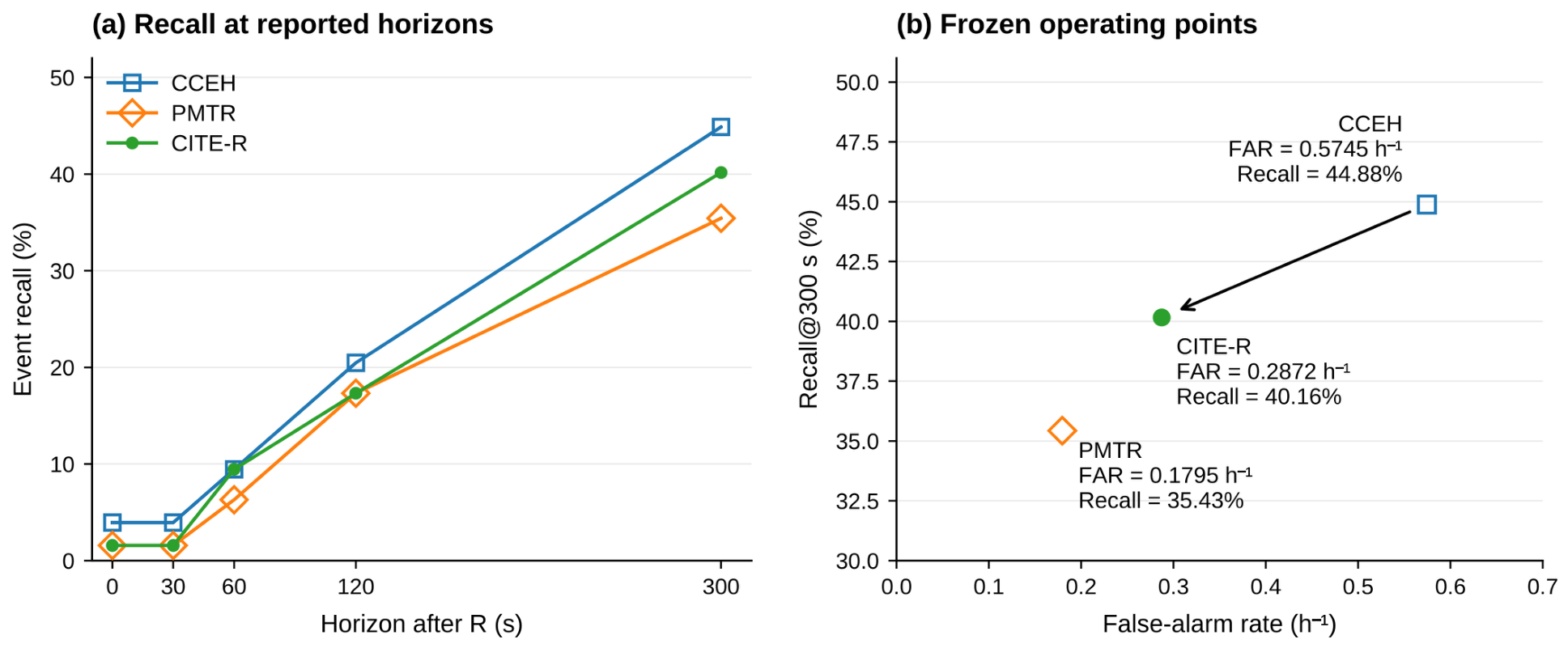
At the validation-frozen operating points, CITE-R detects 51 of 127 FIgLib events within 300 s, compared with 57 for CCEH (Table 2). Over the same negative exposure, false-alarm episodes decrease from 16 to 8 and FAR from 0.5745 to 0.2872 h−1. This represents a 50% reduction in episodes accompanied by a 4.72-percentage-point decrease in event recall. Supplementary Materials Tables S11a and S23 give paired event outcomes and uncertainty estimates.
Table 2.
FIgLib event recall values and false-alarm rates at model-specific validation-frozen thresholds. Recall values are expressed as percentages. FAR uses the same verified negative exposure and 120 s consecutive-alarm merging rule for all methods.
PMTR is more conservative, with 35.43% recall at 300 s and a FAR of 0.1795 h−1. With HSRC, CITE-R increases these to 40.16% and 0.2872 h−1, trading higher sensitivity for more false alarms rather than acting solely as a rejection gate.
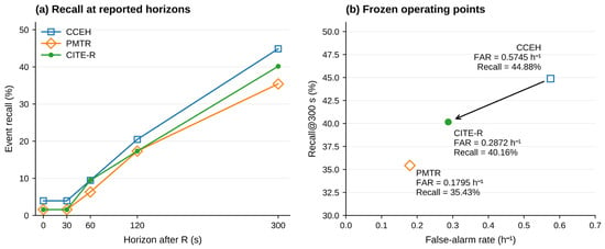
At 60 s, CITE-R and CCEH each detect 9.45% of events, compared with 6.30% for PMTR. Figure 6b shows the associated recall–FAR operating points. These measurements describe how the final correction balances sensitivity and alarm burden after threshold transfer. Supplementary Materials Table S4 reports the archival multiplicative verifier.
Figure 6.
FIgLib source-out performance from Table 2. (a) Event recall at the observed post-R horizons. (b) Recall@300 s and FAR at the model-specific validation-frozen thresholds; the arrow connects the CCEH and CITE-R operating points.
At FAR ceilings of 0.20, 0.30, and 0.40 h−1, the descriptive common-FAR envelope gives recall differences of 0.79–1.57 percentage points in favor of CITE-R; the paired 95% camera-cluster intervals include zero. The complete results are reported in Supplementary Materials Table S48.
Under the same development-negative-unit constraint, the score-only calibration control detects 61 events and produces 44 false-alarm episodes, compared with 51 and 8 for CITE-R. Its training, frozen operating points, and paired comparisons are reported in Supplementary Materials Section S7.8.
The newly trained ResNet50–LSTM verifier detects 45/127 events within 300 s and produces 12 false-alarm episodes, compared with 51/127 and 8 for CITE-R under the shared development calibration rule. Within 60 s, CITE-R detects 12 events, and the LSTM detects six. Supplementary Materials Section S7.17 reports this public-architecture comparison and the simpler presence anchors.
All ten HSRC heads trained with PMTR fixed reduce FAR relative to CCEH. Mean source-out recall is 36.06% ± 5.69 percentage points and mean FAR is 0.2226 ± 0.1099 h−1 (Supplementary Materials Table S11b). These results characterize the sensitivity–false-alarm trade-off across final-head initializations.
3.2. Controlled Physical-Time Comparison
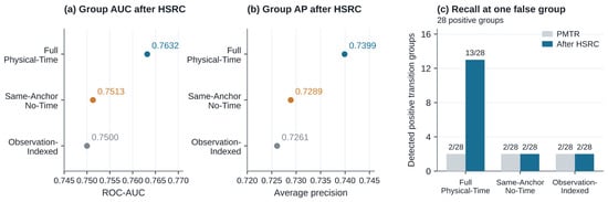
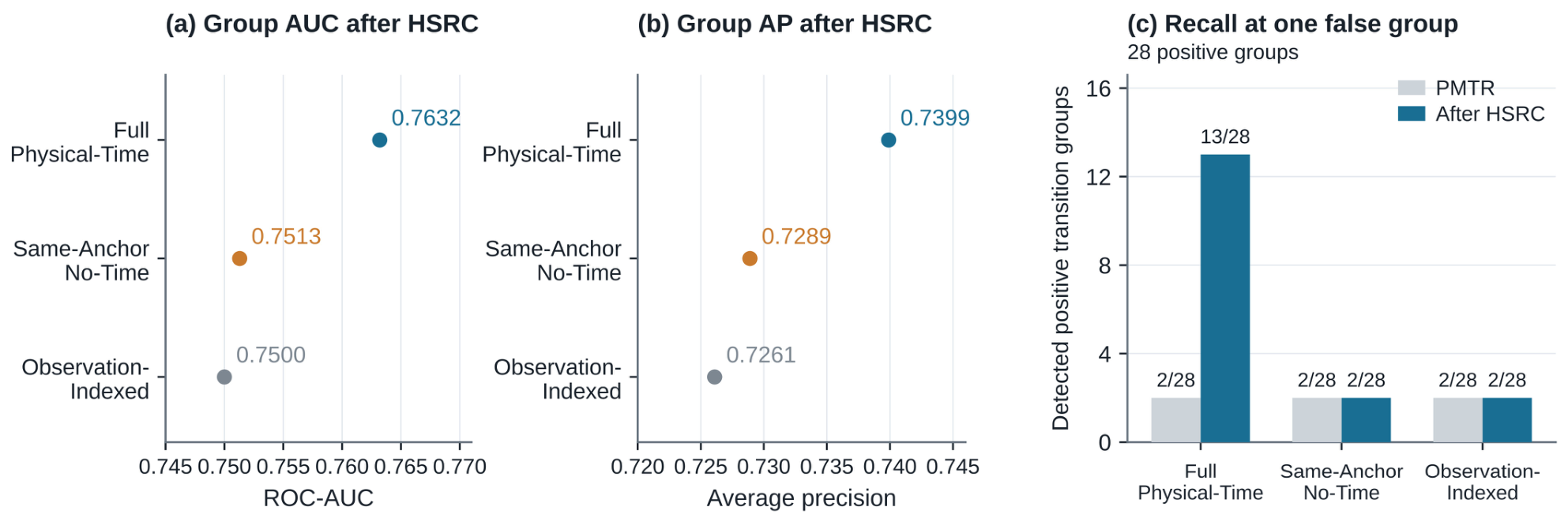
The seed-44 controls examine whether the physical-time design provides benefits beyond access to historical observations (Figure 7). After HSRC, Full Physical-Time achieves a group AUC/AP of 0.7632/0.7399, compared with 0.7513/0.7289 for Same-Anchor No-Time and 0.7500/0.7261 for Observation-Indexed. At one false validation group, the full representation detects 13/28 positive transition groups (46.43%); each alternative detects 2/28 (7.14%). Supplementary Materials Table S13 gives both stage-level results and history coverage.
Figure 7.
Physical-time controls at seed 44. (a,b) Validation group AUC and AP after HSRC. (c) Detected positive transition groups before and after HSRC at one false group, with 28 positives in each comparison. PMTR denotes the representation-stage result (A3); the corresponding HSRC result is A4. These are single-seed transition-group results. In panels (a) and (b), blue denotes Full Physical-Time, orange denotes Same-Anchor No-Time, and gray denotes Observation-Indexed. In panel (c), light-gray bars show the PMTR results before HSRC, and blue bars show the results after HSRC.
The stage comparison identifies where the difference in constrained recall appears. Before HSRC, all three variants detect 2/28 groups, although Full Physical-Time already has higher AUC and AP (Table S13). HSRC improves AUC and AP for all three representations, while the full representation increases constrained hits to 13/28. This result links physical-time features and signed correction at the tested low-false-group operating point.
Full Physical-Time and Same-Anchor No-Time have the same mean coverage of 2.624 valid anchors, compared with 5.359 for Observation-Indexed. These means include the native slot and all 1244 cached records. The indexed history contains substantially older observations (Supplementary Materials Section S7.3). Same-Anchor No-Time tests descriptor-time encoding with matched anchors, whereas Observation-Indexed changes both retrieval coverage and encoding.
Across seeds 40, 41, and 42, matched PMTR–HSRC retraining yields mean FIgLib Recall@300 s after HSRC of 4.72%, 12.86%, and 11.02% for Full Physical-Time, Same-Anchor No-Time, and Observation-Indexed, respectively, at the primary one-of-37 development-negative-unit constraint. The corresponding mean FARs are 0.0838, 0.1317, and 0.0598 h−1. At this budget, Full Physical-Time detects 4, 7, and 7 of the 127 FIgLib events within 300 s for seeds 40, 41, and 42, respectively, with fewer detections than either time control in each matched comparison (Supplementary Materials Table S30). Results across all three calibration budgets are reported in Supplementary Materials Tables S29–S31.
In observation-removal tests with the seed-44 models and thresholds fixed, Full retains higher recall than both time controls, while its recall decreases as observations are removed. These tests use frozen upstream candidate and context features (Supplementary Materials Tables S45 and S46).
3.3. Signed Correction and Supporting Presence Evidence
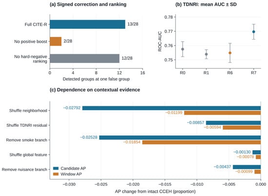
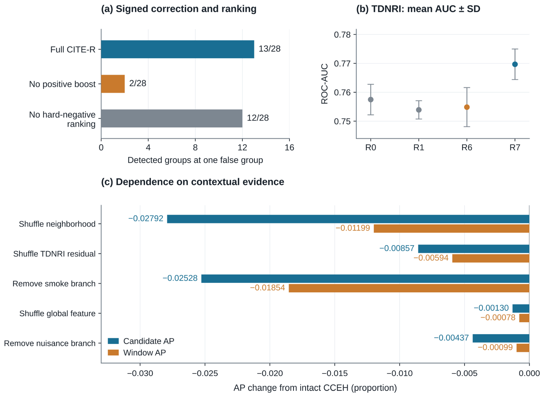
The seed-44 development run improves group AUC/AP from 0.720899/0.677081 for PMTR to 0.763228/0.739896 for CITE-R. Figure 8a examines the two HSRC design choices at one false validation group. Removing positive residual boosting reduces transition-group hits from 13/28 to 2/28, supporting the role of positive correction in this setting. Supplementary Materials Table S7 reports the full validation and source-out metrics.
Figure 8.
Supporting evidence for verification. (a) HSRC ablations at one false validation group, with 28 positive groups. (b) TDNRI mean AUC ± standard deviation over three initializations: R0, no temporal state; R1, adjacent-frame difference; R6, dual states with elapsed time; R7, R6 with candidate protection. (c) Candidate- and window-level AP changes after inference-time interventions on fitted CCEH. Tables S7–S9 give the complete values and evaluation populations.
On FIgLib, enabling signed rather than suppress-only correction raises Recall@300 s from 35.43% to 40.16% and FAR from 0.1795 to 0.2872 h−1. The positive correction mechanism preserves more sensitivity at these transferred thresholds, accompanied by an increase in false alarms.
Removing hard-negative ranking slightly increases validation AUC and AP but reduces constrained hits to 12/28. Its source-out operating point is more conservative, with Recall@300 s of 25.98% and FAR of 0.0718 h−1. Retaining ranking is associated with higher external recall and higher FAR under validation-selected thresholds.
Across three initializations, candidate-protected adaptation has the highest mean AP, AUC, and F1 among the principal TDNRI variants (Figure 8b; Table S8). Relative to adjacent-frame differencing, the absolute gains are 0.00433, 0.01577, and 0.00121. Dual elapsed-time states without protection do not outperform the simpler references on these mean metrics. The result favors the combined protected-adaptation design rather than elapsed-time states alone.
The fitted CCEH is most sensitive to shuffling annular-neighborhood features and removing the local smoke-oriented branch (Figure 8c). TDNRI residual interventions have a smaller effect; global context and the neighborhood–global branch have weaker effects. These inference-time interventions identify dependencies of the learned presence estimate, particularly on local–neighborhood relations. Exact candidate- and window-level changes appear in Table S9.
C5 was retained as the relation-based presence anchor for the correction experiments; the development screening results are given in Supplementary Materials Section S3. In the seed-44 final-alarm comparison at the primary development calibration budget, C4 and C5 use the same frozen R7 features. The simpler C4 presence head detects 62 of 127 events with 13 false-alarm episodes, compared with 57 detections and 16 episodes for CCEH/C5 (Supplementary Materials Table S40).
The matched R6/R7 comparison trains new C5, PMTR, and HSRC heads for each frozen feature generator, with class-balanced BCE for the new presence heads. At the one-of-37 development-negative-unit constraint, the final HSRC stage detects 21 of 127 events with five false-alarm episodes for R6 without protection, compared with one event and one episode for R7 with protection (Supplementary Materials Table S42). This new-head protocol is separate from the original frozen pipeline. All stage results are provided in Supplementary Materials Section S7.17.
3.4. Detection at Reviewed Visibility Boundaries
At a threshold of 0.8958815336, CITE-R detects 14 of 29 reviewed validation events at R and triggers one of 37 reviewed negative units (Table S10). The resulting boundary recall is 48.28%, distinct from the 13/28 transition-group result. Four events trigger alarms before L and nine at L; their union contains 12 events, so the counts overlap.
The boundary analysis shows both detection at the first confirmed visible-smoke observations and premature responses. The 12/29 events with an alarm at or before the reviewed no-smoke boundary are not credited as successful early detections. Moreover, the 1.57% FIgLib R-anchor recall shows that validation-boundary sensitivity does not transfer unchanged under the frozen threshold.
3.5. Nuisance Responses and Real-Scene Behavior
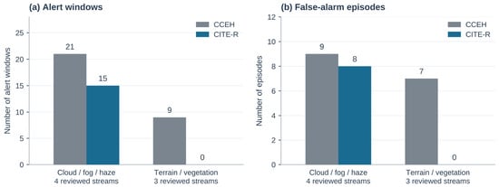
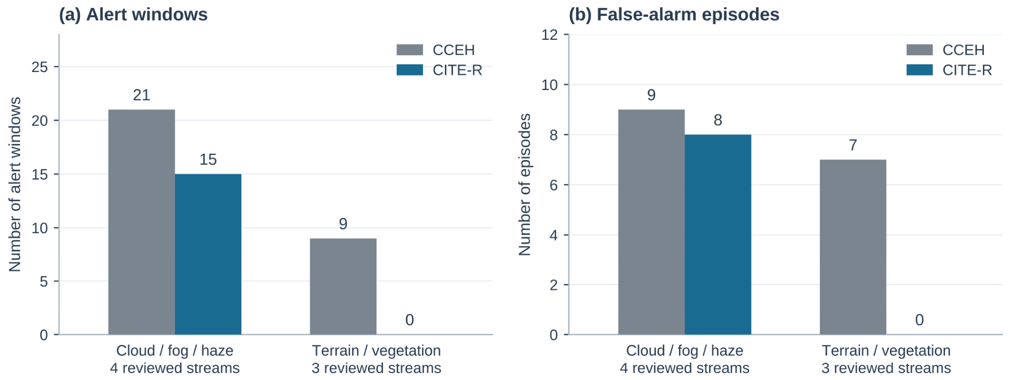
CCEH triggers alarms in 30 windows across seven negative streams, compared with 15 windows across two streams for CITE-R. Figure 9 separates these responses by nuisance type. Terrain/vegetation episodes decrease from seven to zero, while cloud/fog/haze episodes decrease from nine to eight. Seven of the eight removed episodes therefore belong to the terrain/vegetation group.
Figure 9.
Nuisance responses on the seven reviewed negative streams that trigger alarms under either frozen method. (a) Alert windows. (b) False-alarm episodes after the 120 s consecutive-alarm merging rule. The subset contains four cloud/fog/haze streams and three terrain/vegetation streams. Totals for CCEH and CITE-R are 30 versus 15 windows and 16 versus 8 episodes. Supplementary Materials Table S12 gives the per-category counts.
Window and episode counts give complementary information. Atmospheric alert windows fall from 21 to 15, but episodes decrease only slightly, and both streams that continue to trigger CITE-R alarms are atmospheric. The episode reduction is concentrated in the inspected terrain/vegetation cases. Slowly varying atmospheric structures remain difficult to distinguish from smoke.
Spatial association of alarm candidates and S0 proposal coverage are examined in Supplementary Materials Section S7.9, alongside the temporal event metric used in Table 2.
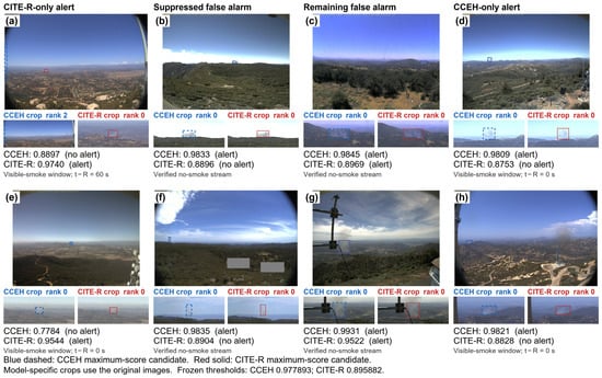
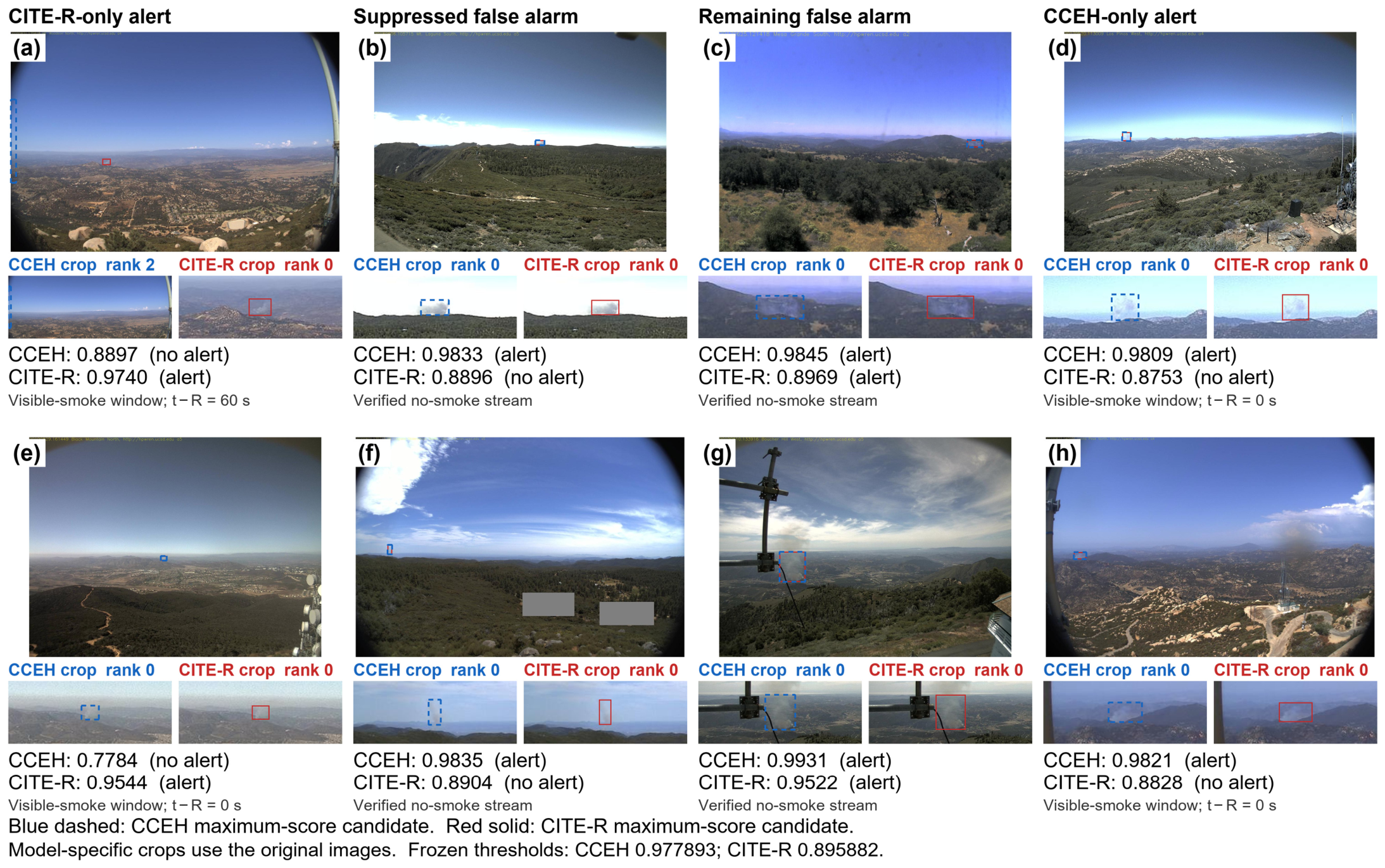
Figure 10 illustrates the frozen-threshold decisions in the same eight real FIgLib windows [7], with each method’s actual maximum-score candidate and corresponding crop shown separately. The figure includes beneficial changes and remaining errors and complements the event-level evaluation and spatial diagnostics.
Figure 10.
Qualitative comparison of CCEH and CITE-R in eight original FIgLib windows [7]. Panels (a,e) show visible-smoke windows in which CITE-R triggers an alarm and CCEH does not; (b,f) show verified no-smoke windows in which CITE-R suppresses CCEH alarms; (c,g) show remaining false alarms; and (d,h) show visible-smoke windows in which CCEH triggers an alarm and CITE-R does not. Blue dashed boxes and blue-labeled crops identify the actual CCEH maximum-score candidate; red solid boxes and red-labeled crops identify the CITE-R maximum-score candidate. Ranks are zero-based, and scores are window maxima. Decisions use the original validation-frozen thresholds of 0.977893 and 0.895882, respectively. Crops use the source images without contrast enhancement. For visible-smoke windows, t−R is the elapsed time from the confirmed visible-smoke observation R.
The method-specific maxima show beneficial changes and remaining errors at the frozen thresholds. False negatives in panels (d) and (h) of Figure 10 refer to the displayed observations; event detection is evaluated over the full 300 s horizon in Table 2. Figure 8a separately tests positive residual boosting using a controlled ablation.
3.6. Complete-Pipeline Computational Profile
On a GeForce RTX 4090 (NVIDIA, Santa Clara, CA, USA), the complete pipeline from raw-image decoding to the final window score averages 70.62 ms at a 1024-pixel input, with a p95 latency of 73.39 ms and throughput of 14.16 target windows/s. At 640 pixels, mean latency is 49.96 ms and throughput is 20.02 target windows/s. Peak allocated GPU memory is 312.26 and 235.97 MiB, respectively. Each measurement uses 90 target windows after warmup; initialization costs, per-module timings, precision, and caching are detailed in Supplementary Materials Section S7.18.
4. Discussion
4.1. Contribution of the Verification Design
The central design choice is to learn a bounded correction to an existing smoke-presence estimate. Physical-time transitions describe changes over unequal observation intervals, while group-level classification and hard-negative ranking connect those features to the alarm objective. A signed correction can strengthen supported weak responses as well as suppress nuisance candidates. This incorporates temporal evidence into the decision rule rather than using it solely as a rejection filter.
The candidate-level TDNRI comparisons favor protected adaptation, while interventions on the fitted CCEH identify a strong contribution from neighborhood context. The archived seed-44 controls support the contributions of positive residual correction and physical-time features when combined with HSRC. Retrained presence and protection comparisons in Supplementary Materials Section S7.17 further distinguish these component-level findings from final alarm behavior, which depends on the trained anchor and operating point.
Separating PMTR and HSRC also separates representation learning from alarm-oriented learning. PMTR summarizes observed transitions, while HSRC learns a bounded update from fixed inputs using group and candidate-level supervision. This allows weak presence scores to be increased while exposing the update to high-scoring nuisance groups.
4.2. Operational Meaning and Source Transfer
The representative source-out operating point eliminates eight false-alarm episodes but results in six fewer detections among 127 events within 300 s. This trade-off is relevant to camera networks where operators verify repeated alarms [5,6]. The observed reduction could lower verification workload, while the recall cost makes the choice of operating point application-dependent. Development data should set that choice according to the intended alarm burden and required sensitivity.
The nuisance breakdown provides a more specific interpretation of the overall FAR change. Most removed episodes involve terrain or vegetation. Atmospheric interference produces fewer alert windows but only a small reduction in episodes. The remaining cloud/fog responses identify an important area for improving scene references and temporal evidence.
Full Physical-Time has the highest mean group AP and AUC on the development set (Supplementary Materials Table S29). These metrics summarize ranking across thresholds. For each calibration budget, the alarm thresholds are selected on development data and held fixed for FIgLib evaluation. The primary budget allows at most one of the 37 development-negative units to trigger an alarm. Under this budget, the models yield different FARs on FIgLib, and Full Physical-Time has lower event recall than both time controls in each of the three matched seeds. At the two-unit budget, its mean Recall@300 s (31.50%) and mean FAR (0.3112 h−1) are higher than those of both controls. Its paired recall difference relative to Same-Anchor No-Time at this budget ranges from −14.17 to +25.20 percentage points across seeds (Supplementary Materials Tables S30 and S31).
4.3. Scope and Limitations
The evaluation is limited to daytime RGB monitoring with approximately stable viewpoints and the frozen S0 proposal generator. TDNRI constructs window-local references over four observations. Its time constants specify adaptation rates within that history. Mobile or substantially moving cameras, nighttime imagery, and infrared sensing require separate evaluation.
The 22 negative streams provide a measured sample of nuisance conditions, and sparse observations limit temporal resolution. Onset boundaries and negative-stream labels were reviewed by the first author; blinding could not be verified from the retained records, and inter-rater agreement was not assessed. Different judgments about the first visible-smoke observation could shift the 300 s evaluation window and change which alarms count as event hits. The choice of smoke-free streams can affect both the number of false-alarm episodes and the covered camera-hours used to calculate FAR. Recalculating recall and FAR after independent review of the same videos would quantify the effect of annotation decisions. Evaluation on additional camera networks would test whether the observed recall–FAR trade-off holds under different nuisance conditions. Supplementary Materials Sections S2, S7.6, and S7.16 document the data populations and source checks; Section S7.4 describes the manual review; and Section S7.9 gives the spatial alarm diagnostics. The matched-retraining analysis in Section S7.11 quantifies variation beyond the original ten-head study with fixed PMTR.
The computational profile applies to the tested implementation and hardware. Event accuracy was evaluated at 1024 pixels; the 640-pixel run measures runtime only. The missing-observation analysis evaluates temporal verification with frozen upstream candidate and context features (Supplementary Materials Sections S7.18 and S7.19).
5. Conclusions
This study presents a candidate-anchored verification framework for fixed-view forest smoke monitoring. CITE-R combines physical-time transition features with a bounded signed update to a contextual presence logit. Candidate-protected reference adaptation and local–neighborhood–scene relations provide the presence anchor; group and candidate-level supervision connect its temporal correction to alarm decisions.
In the seed-44 development comparison, the full physical-time design achieves 13/28 transition-group hits, compared with 2/28 after removing positive corrections or using either time-ablated alternative under the same false-group allowance. At the validation-frozen FIgLib thresholds, CITE-R reduces false-alarm episodes from 16 to 8 over 27.8506 camera-hours, while 300 s event hits decrease from 57 to 51 out of 127. All ten HSRC initializations with PMTR fixed reduce FAR relative to CCEH, with varying decreases in recall. In matched PMTR–HSRC retraining, Full Physical-Time has lower FIgLib event recall than both time controls for all three seeds at the primary budget. At the two-unit budget, its mean recall and FAR are higher than those of both controls, and it detects more events than Same-Anchor No-Time in two of the three seeds. The measured pipeline latency of 70.62 ms at a 1024-pixel input supports near-real-time verification on the tested RTX 4090.
The framework provides a physical-time-conditioned signed correction for managing the sensitivity–false-alarm trade-off in fixed-view monitoring, with transferred operating points depending on the development calibration budget. Future work will examine motion and persistence cues and scene-conditioned reference modeling to distinguish slowly evolving cloud and fog structures from emerging smoke.
Supplementary Materials
The following supporting information can be downloaded at https://www.mdpi.com/article/10.3390/fire9110520/s1. The accompanying document provides implementation details (S1), resource inventories (S2), development comparisons (S3), detector profiles (S4), operating-point diagnostics (S5), supporting results (S6), and additional protocols and analyses (S7). Sections S7.16–S7.21 cover source identifiers, matched temporal and presence baselines, complete-pipeline profiling, controlled missing observations, training reproduction, and common-FAR uncertainty. Tables S1–S48 and the companion records provide the complete results. Reference [36] is cited in the Supplementary Materials.
Author Contributions
Conceptualization, H.S. and W.L.; Methodology, H.S.; Software, H.S.; Validation, H.S.; Formal analysis, H.S.; Investigation, H.S.; Data curation, H.S.; Writing—original draft preparation, H.S.; Writing—review and editing, W.L. and X.S.; Visualization, H.S.; Supervision, W.L.; Project administration, W.L. All authors have read and agreed to the published version of the manuscript.
Funding
This research received no external funding.
Institutional Review Board Statement
Not applicable.
Informed Consent Statement
Not applicable.
Data Availability Statement
Third-party datasets, including Pyro-SDIS, PyroNear2025, and FIgLib, can be obtained from their original sources under their respective terms. Code and reproducibility materials are publicly archived on Zenodo as version 1.0.1 [37] at https://doi.org/10.5281/zenodo.24154640, including implementations, configurations, trained weights, training/evaluation scripts, protocols, environment information, and reference results. Additional revision scripts, selected comparison heads, frozen thresholds, and compact results tables accompany the supplementary records. Third-party images and large generated feature databases are not redistributed.
Acknowledgments
During the preparation of this study, the authors used ChatGPT (OpenAI, GPT-5.6 Sol) for English language editing and polishing and to assist with generating flowcharts and explanatory workflow/architecture diagrams. The authors reviewed and edited all AI-assisted outputs and take full responsibility for the content of this publication.
Conflicts of Interest
The authors declare no conflicts of interest.
Abbreviations
TDNRI: Time-aware dual-timescale normality adaptation (module label). CCEH: Candidate–context evidence head. PMTR: Physical-time multiscale transition representation. HSRC: Hard-negative signed residual calibration. CITE-R: PMTR–HSRC correction stage applied to the contextual presence anchor (method label). AP: Average precision; AUC: Area under the ROC curve; FAR: False-alarm rate; IoU: Intersection over union; ROI: Region of interest.
References
- Chaturvedi, S.; Khanna, P.; Ojha, A. A survey on vision-based outdoor smoke detection techniques for environmental safety. ISPRS J. Photogramm. Remote Sens. 2022, 185, 158–187. [Google Scholar] [CrossRef] [Scilit]
- Cheng, G.; Chen, X.; Wang, C.; Li, X.; Xian, B.; Yu, H. Visual fire detection using deep learning: A survey. Neurocomputing 2024, 596, 127975. [Google Scholar] [CrossRef] [Scilit]
- Gragnaniello, D.; Greco, A.; Sansone, C.; Vento, B. Fire and smoke detection from videos: A literature review under a novel taxonomy. Expert Syst. Appl. 2024, 255, 124783. [Google Scholar] [CrossRef] [Scilit]
- Fernandes, A.M.; Utkin, A.B.; Chaves, P. Automatic early detection of wildfire smoke with visible light cameras using deep learning and visual explanation. IEEE Access 2022, 10, 12814–12828. [Google Scholar] [CrossRef] [Scilit]
- Fernandes, A.M.; Utkin, A.B.; Chaves, P. Automatic early detection of wildfire smoke with visible-light cameras and EfficientDet. J. Fire Sci. 2023, 41, 122–135. [Google Scholar] [CrossRef] [Scilit]
- Govil, K.; Welch, M.L.; Ball, J.T.; Pennypacker, C.R. Preliminary results from a wildfire detection system using deep learning on remote camera images. Remote Sens. 2020, 12, 166. [Google Scholar] [CrossRef] [Scilit]
- Dewangan, A.; Pande, Y.; Braun, H.-W.; Vernon, F.; Perez, I.; Altintas, I.; Cottrell, G.W.; Nguyen, M.H. FIgLib & SmokeyNet: Dataset and deep learning model for real-time wildland fire smoke detection. Remote Sens. 2022, 14, 1007. [Google Scholar] [CrossRef] [Scilit]
- Yazdi, A.; Qin, H.; Jordan, C.B.; Yang, L.; Yan, F. Nemo: An open-source transformer-supercharged benchmark for fine-grained wildfire smoke detection. Remote Sens. 2022, 14, 3979. [Google Scholar] [CrossRef] [Scilit]
- Lostanlen, M.; Isla, N.; Guillén, J.; Zanca, R.; Veith, F.; Buc, C.; Barriere, V. A real-world benchmark for early wildfire detection using sequential data with the PyroNear dataset. Electronics 2026, 15, 2652. [Google Scholar] [CrossRef] [Scilit]
- Wang, C.; Song, H.; Wang, Z.; Shan, Z.; Zhang, Q. LwST-FSD: Efficient forest smoke detection via lightweight spatio-temporal modeling. Inf. Sci. 2025, 719, 122481. [Google Scholar] [CrossRef] [Scilit]
- Gubbi, J.; Marusic, S.; Palaniswami, M. Smoke detection in video using wavelets and support vector machines. Fire Saf. J. 2009, 44, 1110–1115. [Google Scholar] [CrossRef] [Scilit]
- Jakovčević, T.; Stipaničev, D.; Krstinić, D. Visual spatial-context based wildfire smoke sensor. Mach. Vis. Appl. 2013, 24, 707–719. [Google Scholar] [CrossRef] [Scilit]
- Peng, Y.; Wang, Y. Real-time forest smoke detection using hand-designed features and deep learning. Comput. Electron. Agric. 2019, 167, 105029. [Google Scholar] [CrossRef] [Scilit]
- Khan, S.; Muhammad, K.; Hussain, T.; Del Ser, J.; Cuzzolin, F.; Bhattacharyya, S.; Akhtar, Z.; de Albuquerque, V.H.C. DeepSmoke: Deep learning model for smoke detection and segmentation in outdoor environments. Expert Syst. Appl. 2021, 182, 115125. [Google Scholar] [CrossRef] [Scilit]
- Zheng, X.; Chen, F.; Lou, L.; Cheng, P.; Huang, Y. Real-time detection of full-scale forest fire smoke based on deep convolution neural network. Remote Sens. 2022, 14, 536. [Google Scholar] [CrossRef] [Scilit]
- Hu, Y.; Zhan, J.; Zhou, G.; Chen, A.; Cai, W.; Guo, K.; Hu, Y.; Li, L. Fast forest fire smoke detection using MVMNet. Knowl.-Based Syst. 2022, 241, 108219. [Google Scholar] [CrossRef] [Scilit]
- Li, J.; Zhou, G.; Chen, A.; Lu, C.; Li, L. BCMNet: Cross-layer extraction structure and multiscale downsampling network with bidirectional transpose FPN for fast detection of wildfire smoke. IEEE Syst. J. 2023, 17, 1235–1246. [Google Scholar] [CrossRef] [Scilit]
- Li, R.; Hu, Y.; Li, L.; Guan, R.; Yang, R.; Zhan, J.; Cai, W.; Wang, Y.; Xu, H.; Li, L. SMWE-GFPNNet: A high-precision and robust method for forest fire smoke detection. Knowl.-Based Syst. 2024, 289, 111528. [Google Scholar] [CrossRef] [Scilit]
- Zhao, Y.; Lv, W.; Xu, S.; Wei, J.; Wang, G.; Dang, Q.; Liu, Y.; Chen, J. DETRs beat YOLOs on real-time object detection. In Proceedings of the IEEE/CVF Conference on Computer Vision and Pattern Recognition (CVPR), Seattle, WA, USA, 16 September 2024; pp. 16965–16974. [Google Scholar] [CrossRef] [Scilit]
- Jung, G.; Ahn, T.-H.; Min, B. Early wildfire smoke detection with a multi-resolution framework and two-stage classification pipeline. Fire 2026, 9, 92. [Google Scholar] [CrossRef] [Scilit]
- Wang, C.; Xu, C.; Akram, A.; Wang, Z.; Shan, Z.; Zhang, Q. Wildfire smoke detection system: Model architecture, training mechanism, and dataset. Int. J. Intell. Syst. 2025, 2025, 1610145. [Google Scholar] [CrossRef] [Scilit]
- Fernandes, A.; Utkin, A.; Chaves, P. Enhanced automatic wildfire detection system using big data and EfficientNets. Fire 2024, 7, 286. [Google Scholar] [CrossRef] [Scilit]
- Tao, H.; Duan, Q.; Lu, M.; Hu, Z. Learning discriminative feature representation with pixel-level supervision for forest smoke recognition. Pattern Recognit. 2023, 143, 109761. [Google Scholar] [CrossRef] [Scilit]
- Tao, H. A label-relevance multi-direction interaction network with enhanced deformable convolution for forest smoke recognition. Expert Syst. Appl. 2024, 236, 121383. [Google Scholar] [CrossRef] [Scilit]
- Ghimire, D.; Kim, D.; Jo, Y.; Lee, E.; Jeong, S.; Kim, B. STV-FSANet: Track-level spatio-temporal verification for fire and smoke alarm validation in video surveillance. Sensors 2026, 26, 4970. [Google Scholar] [CrossRef] [Scilit] [PubMed]
- Cao, Y.; Yang, F.; Tang, Q.; Lu, X. An attention enhanced bidirectional LSTM for early forest fire smoke recognition. IEEE Access 2019, 7, 154732–154742. [Google Scholar] [CrossRef] [Scilit]
- Cao, Y.; Tang, Q.; Wu, X.; Lu, X. EFFNet: Enhanced feature foreground network for video smoke source prediction and detection. IEEE Trans. Circuits Syst. Video Technol. 2022, 32, 1820–1833. [Google Scholar] [CrossRef] [Scilit]
- Tao, H.; Duan, Q. An adaptive frame selection network with enhanced dilated convolution for video smoke recognition. Expert Syst. Appl. 2023, 215, 119371. [Google Scholar] [CrossRef] [Scilit]
- Tao, H. A triple interference removal network based on temporal and spatial attention interaction for forest smoke recognition in videos. Comput. Electron. Agric. 2024, 218, 108756. [Google Scholar] [CrossRef] [Scilit]
- Krstinić, D.; Bejo, J.; Sikora, T.; Bugarić, M. Spatio-temporal data model for early wildfire detection. Fire 2026, 9, 175. [Google Scholar] [CrossRef] [Scilit]
- Bhamra, J.K.; Anantha Ramaprasad, S.; Baldota, S.; Luna, S.; Zen, E.; Ramachandra, R.; Kim, H.; Schmidt, C.; Arends, C.; Block, J.; et al. Multimodal Wildland Fire Smoke Detection. Remote Sens. 2023, 15, 2790. [Google Scholar] [CrossRef] [Scilit]
- Muksimova, S.; Umirzakova, S. Detecting Wildfire Smoke Onset from Fixed View Camera Networks. Sensors 2026, 26, 6020. [Google Scholar] [CrossRef] [Scilit] [PubMed]
- Che, Z.; Purushotham, S.; Cho, K.; Sontag, D.; Liu, Y. Recurrent neural networks for multivariate time series with missing values. Sci. Rep. 2018, 8, 6085. [Google Scholar] [CrossRef] [Scilit] [PubMed]
- PyroNear. Pyro-SDIS. Hugging Face Dataset. Available online: https://huggingface.co/datasets/pyronear/pyro-sdis (accessed on 6 November 2026).
- Ultralytics. Ultralytics YOLO11. Available online: https://docs.ultralytics.com/models/yolo11/ (accessed on 6 November 2026).
- Jocher, G.; Qiu, J.; Liu, M.; Lyu, S.; Akyon, F.C.; Kalfaoglu, M.E. Ultralytics YOLO26: Unified Real-Time End-to-End Vision Models. arXiv 2026, arXiv:2606.03748. [Google Scholar] [CrossRef] [Scilit]
- Sun, H. Code and Reproducibility Materials for Physical-Time Signed Residual Calibration for Fixed-View Forest Smoke Detection, Version 1.0.1; Zenodo: Geneva, Switzerland, 2026. [CrossRef]

Disclaimer/Publisher’s Note: The statements, opinions and data contained in all publications are solely those of the individual author(s) and contributor(s) and not of MDPI and/or the editor(s). MDPI and/or the editor(s) disclaim responsibility for any injury to people or property resulting from any ideas, methods, instructions or products referred to in the content. |
© 2026 by the authors. Licensee MDPI, Basel, Switzerland. This article is an open access article distributed under the terms and conditions of the Creative Commons Attribution (CC BY) license.