Deep Learning-Based Reconstruction of Particle Beam Energy Spectra from Attenuation Curve Data

Abstract

This paper introduces a deep learning-based methodology for reconstructing particle beam energy spectra from experimental attenuation curves. This task involves solving a classic ill-posed inverse problem for a Fredholm integral equation of the first kind. Unlike traditional Arsenin–Tikhonov regularization, the proposed framework utilizes two coupled neural networks for spectrum approximation and adaptive kernel correction. This approach explicitly accounts for measurement uncertainties in the experimental data. As a mesh-free technique, it operates directly on raw sparse experimental datasets without preprocessing. Validation using data from subnanosecond electron beams in gas-filled and vacuum diodes demonstrates that the method successfully resolves non-trivial two-peak spectral structures. In particular, it reliably identifies populations of “anomalous” high-energy electrons that are often obscured by classical regularization artifacts.

1. Introduction

The experimental determination of particle energy distribution functions in beams of high-energy electrons, ions, or neutral particles at the output of accelerator systems constitutes a critically important problem in modern applied and fundamental physics [1]. One particularly relevant example of research in this area is the characterization of the energy properties of subnanosecond electron beams. Such beams are generated in pulsed vacuum and gas diodes, and the interest in them is driven by their applications across various fields of science and technology, since their spectral energy distribution exhibits a nontrivial multi-peaked structure.

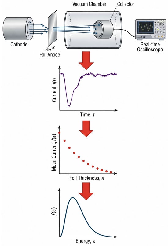
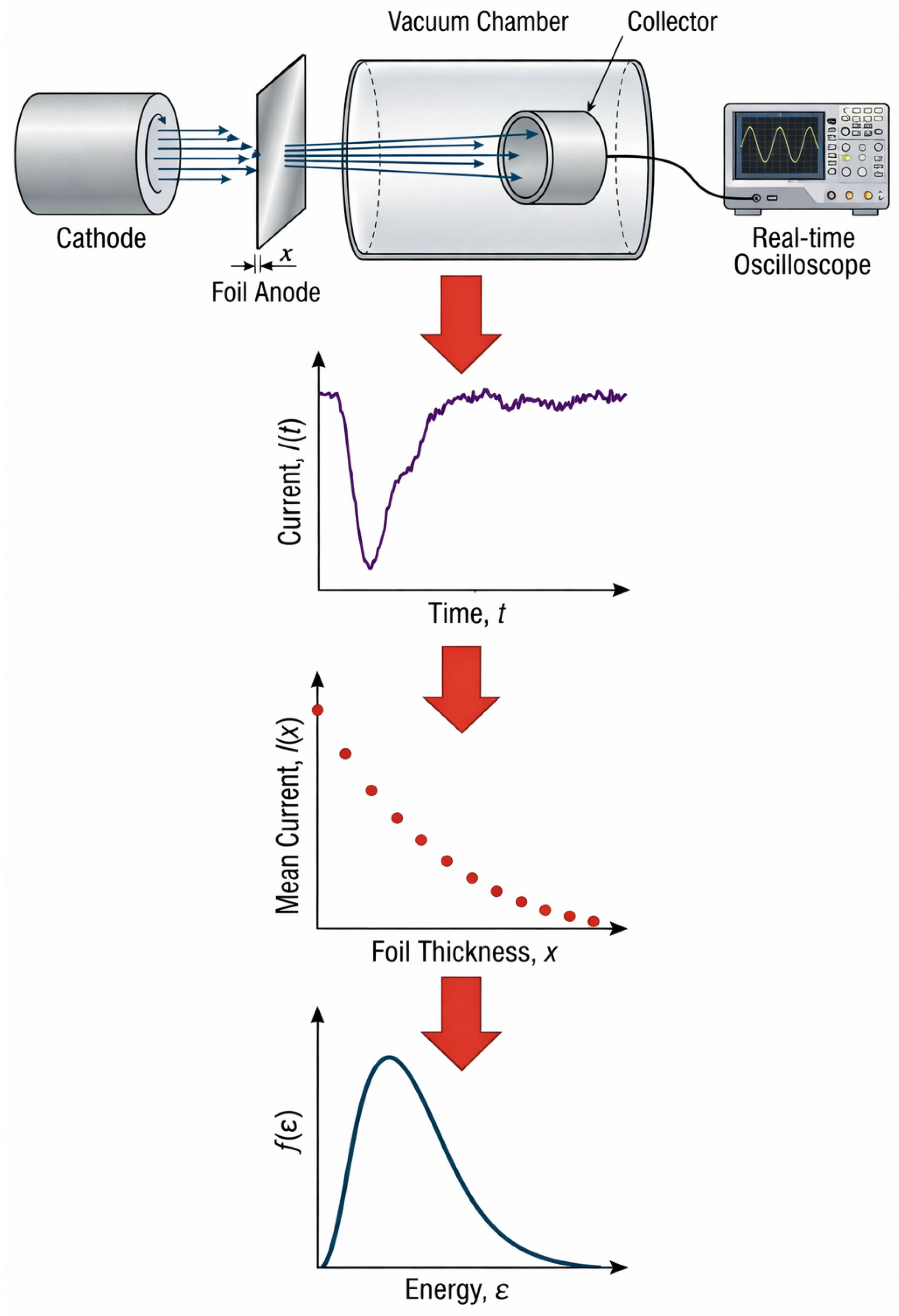
One of the direct methods for measuring particle energy distribution functions f(ε) (hereafter referred to as energy spectra) as a function of energy ε is the use of spectrometer–analyzers [2]. Another widely used approach is the attenuation curve method (e.g., [3,4]), the schematic diagram of which (e.g., for electrons) is shown in Figure 1. Thin, precisely aligned metallic foils of varying thickness are placed behind the accelerator exit window, e.g., the anode of a pulsed gas or vacuum diode. The current collector (Faraday cup) and the recording instrument (real-time oscilloscope) are installed behind the foils inside a vacuum chamber. For each foil of thickness x, the collector current waveform is measured, and its integral characteristic, such as the mean current or the total beam charge, is evaluated. The attenuation curve g(x) is defined, therefore, as the discrete dependence of the current integral characteristic on the foil thickness.

Figure 1. Schematic representation of the reconstruction of the spectral energy distribution of an electron beam using the attenuation curve method.

After obtaining the attenuation curve, the reconstruction of the beam energy spectrum f(ε) reduces to the numerical solution of the following equation:

$${\displaystyle {\displaystyle \underset{{\epsilon }_{\min }}{\overset{{\epsilon }_{\max }}{\int }}}K\left(x,\epsilon \right)f\left(\epsilon \right)d\epsilon =g\left(x\right)},$$

(1)

where the integral equation kernel, i.e., K(x, ε), denotes the known attenuation function for a monoenergetic electron beam of energy ε in a metallic foil of thickness x, and ε_max and ε_min define the energy range considered for the beam.

In addition to the fact that experiments aimed at constructing attenuation curves require a high degree of reproducibility of the experimental conditions, there exists another problem directly associated with solving Equation (1). Specifically, a reliable and physically meaningful solution of this equation cannot be defined as an arbitrary function f(ε) that merely minimizes the residual of the right-hand side in the sense of the L² norm

$${‖{\displaystyle {\displaystyle \underset{{\epsilon }_{\min }}{\overset{{\epsilon }_{\max }}{\int }}}K\left(x,\epsilon \right)f\left(\epsilon \right)d\epsilon -g\left(x\right)}‖}^2<\delta ,$$

where δ is the accuracy constant. The solution can be considered valid only if the corresponding f(ε) is stable with respect to small variations both in the attenuation curve g(x) data and in the kernel of the integral operator K(x, ε) itself. This class of problems is commonly referred to as ill-posed problems of mathematical physics [5]. In the case considered in this work, both g(x) and K(x, ε) are experimental quantities obtained with finite measurement uncertainty

$$\begin{array}{c}g(x)=\overline{g}(x)\pm \Delta g(x),\\ K\left(x,\epsilon \right)=\overline{K}\left(x,\epsilon \right)\pm \Delta K\left(x,\epsilon \right),\end{array}$$

(2)

where both quantities are represented as discrete or approximated sets of mean values, specified with an accuracy limited by the experimental measurement uncertainty.

A method for solving ill-posed problems was proposed and rigorously justified in the monograph by Arsenin and Tikhonov [5]. It is based on introducing a so-called smoothing functional for Equation (1) and minimizing it. As a result, a regularization equation is obtained, which takes the form of a high-order integro-differential equation. By solving this equation using conventional numerical methods, it is possible to reconstruct f(ε) in a manner that is stable with respect to variations in g(x).

Much later, this approach was successfully applied for the first time to reconstruct the spectral energy characteristics of subnanosecond electron beams generated in high-pressure vacuum and gas diodes [6,7,8]. Based on the reconstructed electron energy spectra, important conclusions were drawn regarding the energy structure of short electron beams in both vacuum and gas discharges. In particular, the hypothesis of an extended high-energy distribution function “tail”, extending beyond the maximum corresponding to the diode voltage amplitude, was confirmed. In gas discharges, this phenomenon is associated with runaway electrons possessing anomalously high energies in a nanosecond atmospheric-pressure gas discharge under conditions of strong overvoltage relative to the breakdown voltage [9,10]. The mechanism of the “anomalous” electrons generation in vacuum discharges has also been explained theoretically elsewhere [11].

Although the results of energy spectrum reconstruction using the Arsenin–Tikhonov approach were supported by theoretical models that predict the form of the distribution function f(ε), several important issues remained beyond the scope of the experimental methodology and require further detailed investigation:

• In the methodology of papers [7,8], it was assumed that the kernel of the integral operator K(x, ε) was known exactly. However, it is well established that this kernel is given by the Tabata–Ito formula [12], which itself was obtained through approximation of experimental datasets, so it contains an inaccuracy in the form of measurement error, i.e., (2);
• The transition from the original inverse problem (1) to the Tikhonov regularization equation (or equations) is always associated with the appearance of extra boundary conditions at the endpoints of the ε interval for f(ε) and its derivatives. The specific form of these boundary conditions directly influences the shape of the reconstructed energy spectrum;
• In the most general case, both the attenuation curve and the kernel are represented as discrete sets of data points with known confidence intervals of measurement uncertainty. Any attempt to expand the experimental dataset using interpolation methods introduces additional artificial refining structures into the reconstructed energy spectra.

All of the factors listed above introduce ambiguities into the resulting f(ε). This study aims to resolve those ambiguities by treating the full ill-posed inverse problem of spectrum reconstruction using deep-learning methods. The proposed approach explicitly accounts for measurement uncertainties in both g(x) and K(x, ε) and quantifies their influence on the shape of the reconstructed particle energy spectrum. The results not only yield a robust reconstruction methodology demonstrated on electron beams from vacuum and gas diodes, but also enable the use of severely noise-limited, sparse experimental datasets to identify trends in the energy spectrum that could become observable structures with future improvements in measurement precision.

2. Problem Formulation

The previously employed method (Arsenin–Tikhonov) has been used to reconstruct the energy spectrum from attenuation curve g(x) data obtained with experimental uncertainty. The kernel of the integral operator was assumed to be known exactly. The method consisted of minimizing the following smoothing functional:

$$\begin{array}{c}{M}_1^{\Lambda }={\rho }_{L_2}^2\left(Kf,g\right)+\Lambda \Omega ,\\ {\rho }_{L_2}^2\left(Kf,g\right)\equiv \left|{\displaystyle {\displaystyle \underset{{\epsilon }_{\min }}{\overset{{\epsilon }_{\max }}{\int }}}K\left(x,\epsilon \right)f\left(\epsilon \right)d\epsilon -g\left(x\right)}\right|,\\ \Omega \equiv {\displaystyle {\displaystyle \underset{{\epsilon }_{\min }}{\overset{{\epsilon }_{\max }}{\int }}}\left\{q\left(\epsilon \right)f^2\left(\epsilon \right)+p\left(\epsilon \right){\left(\frac{\mathsf{\partial }f\left(\epsilon \right)}{\mathsf{\partial }\epsilon }\right)}^2\right\}d\epsilon ,}\end{array}$$

where p(ε) and q(ε) are arbitrary weighting functions for the zeroth- and first-order derivatives, respectively.

The minimization of the smoothing functional was carried out by taking its variational derivative and setting it equal to zero. This procedure yielded an integro-differential equation

$$\begin{array}{c}\Lambda \left\{q\cdot f\left(\epsilon \right)-p\cdot f^{″}\left(\epsilon \right)\right\}+{\displaystyle {\displaystyle \underset{{\epsilon }_{\min }}{\overset{{\epsilon }_{\max }}{\int }}}\tilde{K}\left(\epsilon ,\tilde{\epsilon }\right)}f\left(\tilde{\epsilon }\right)d\tilde{\epsilon }=\tilde{g}\left(\epsilon \right),\\ \tilde{K}\left(\epsilon ,\tilde{\epsilon }\right)={\displaystyle {\displaystyle \underset{x_{\min }}{\overset{x_{\max }}{\int }}}K\left(x,\epsilon \right)K\left(x,\tilde{\epsilon }\right)dx},\hspace{0.33em}\tilde{g}(\epsilon )={\displaystyle {\displaystyle \underset{x_{\min }}{\overset{x_{\max }}{\int }}}K\left(x,\epsilon \right)g\left(x\right)dx},\end{array}$$

(3)

which was subsequently solved numerically using grid methods [5]. As a result, energy spectra were obtained that were stable with respect to the attenuation curve g(x) variations within the bounds of the experimental measurement uncertainty.

In the present work, the full inverse problem associated with Equation (1) is addressed; i.e., the kernel of the integral operator K(x, ε) is also assumed to be known only within a prescribed experimental uncertainty (2). Accordingly, to obtain a regularized solution, the following functional must be minimized:

$$M_2^{{\Lambda }_1,{\Lambda }_2}=M_1^{{\Lambda }_1}+{\Lambda }_2\Psi ,\hspace{0.33em}\hspace{0.33em}\Psi \equiv {\displaystyle {\displaystyle \underset{{\epsilon }_{\min }}{\overset{{\epsilon }_{\max }}{\int }}}{\displaystyle {\displaystyle \underset{x_{\min }}{\overset{x_{\max }}{\int }}}{K}^2\left(x,\epsilon \right)dxd\epsilon },}$$

(4)

where the additional term represents the Frobenius norm of the integral operator kernel evaluated over the range of energies and foil thicknesses used in the experiment.

Instead of the conventional approach based on deriving the regularization equation via the calculus of variations, the present work employs a different methodological framework to minimize (4) in the presence of uncertainties of the form (2). This framework relies on deep neural network training techniques, in which the functional (4) is associated with the following composite, normalized loss function

$$\begin{array}{c}\aleph (\theta )={\displaystyle \frac{{\displaystyle \sum _{i=1}^N{\left|{\displaystyle {\displaystyle \underset{{\epsilon }_{\min }}{\overset{{\epsilon }_{\max }}{\int }}}K\left(x_i,\epsilon \right)f_{\theta }\left(\epsilon \right)d\epsilon -g\left(x_i\right)}\right|}^2}}{{\displaystyle \sum _{i=1}^N{\left|g\left(x_i\right)\right|}^2+\delta }}}+\\ +{\lambda }_1{\displaystyle \frac{{\displaystyle \sum _{j=1}^M\left[f_{\theta }{\left({\epsilon }_j\right)}^2+{\displaystyle f_{\theta }^{\prime }}{\left({\epsilon }_j\right)}^2\right]}}{{\displaystyle \sum _{j=1}^M{\left|f_{\theta }\left({\epsilon }_j\right)\right|}^2+\delta }}}+{\lambda }_2\left({\displaystyle \frac{1}{MN}}{\displaystyle \sum _{i=1}^N{\displaystyle \sum _{j=1}^M\Delta K{\left(x_i,{\epsilon }_j\right)}^2}}\right),\end{array}$$

(5)

where θ denotes the set of machine learning parameters (trainable weights and biases), N is the number of experimental data points comprising the attenuation curve, M is the number of nodes in a uniform grid defined over the prescribed energy range, and δ is a small positive constant introduced to prevent singularities in the denominators during normalization of the individual loss terms.

This approach employs two coupled neural networks. The first is a spectrum-approximation network. It consists of three fully connected layers, with 128 neurons in each hidden layer and hyperbolic tangent (“tanh”) activation functions. A “softplus” activation function is used in the output layer to enforce non-negativity of the reconstructed spectrum. Batch normalization is intentionally omitted to ensure the correct computation of higher-order derivatives during automatic differentiation. The second network is a kernel-correction network. It takes the parameters (x, ε) as input and computes an adaptive correction term ΔK, thereby forming the complete kernel in accordance with expression (2). The choice of the “softplus” activation function in the output layer is physically motivated to enforce the non-negativity of the energy spectrum f(ε). Furthermore, the regularization term Ω ensures the smoothness of the solution, serving a similar role to the second-order stabilizer in Tikhonov’s functional but without the need for explicit boundary conditions at the energy interval endpoints.

The numerical integration of the Fredholm operator is performed using Gauss-Legendre quadrature, a high-order spectral method that provides exponential convergence for smooth integrands. The quadrature nodes and weights are computed by solving an eigenvalue problem associated with the Jacobi matrix of Legendre polynomial recurrence coefficients, ensuring optimal accuracy within the computational domain. The quadrature points are deployed across the energy interval [0.05, 0.5] MeV. The integral evaluation is implemented as a weighted summation, where the precomputed weights remain fixed throughout training, enabling efficient forward passes while maintaining mathematical rigor. This approach transforms the continuous integral operator into a discrete linear operation compatible with automatic differentiation frameworks, allowing gradients to flow seamlessly through both the neural network and the physical model during backpropagation.

The training protocol for both neural networks employs the Adam optimizer within Mathworks MATLAB’s Deep Learning Toolbox (R2025b), with automatic differentiation enabled via the “dlfeval” function to ensure stable gradient computation through the composite physics-informed loss function. Convergence was monitored via the composite loss function (5). The training was terminated after 20,000 epochs as the loss reached a stable plateau, with the relative change in the mean squared error (MSE) between epochs falling below 10⁻⁶. This extended schedule ensures that the regularization and data-fidelity terms are optimally balanced. This extended training duration, implemented through a straightforward iterative loop with progress monitoring every 200 epochs, guarantees convergence to a minimizer that balances data fidelity with regularization constraints.

The method’s principal advantages over traditional approaches are its fully mesh-free formulation within MATLAB’s numerical environment, which eliminates spatial discretization errors while leveraging native matrix operations for efficient quadrature evaluation, and its unified differentiable framework that seamlessly integrates MATLAB’s neural network approximator with the physical integral operator. Unlike classical regularization methods that require explicit matrix inversions and specialized optimization toolboxes, this neural network-based approach, implemented in standard MATLAB, implicitly enforces solution smoothness and non-negativity through architectural choices and loss function design, while simultaneously handling data noise and kernel uncertainties through adaptive regularization terms, resulting in enhanced robustness for ill-posed inverse problems with minimal reliance on external computational libraries.

3. Reconstruction of the Electron Spectral Energy Distributions

In this section, we demonstrate reconstruction of the electron energy spectrum from attenuation-curve data measured in aluminum foils, using the same experimental datasets as input. For this procedure, we employ the well-known Tabata–Ito formula [12]:

$$\begin{array}{c}K\left(x,\epsilon ,Z\right)={\displaystyle \frac{1+\exp \left(-\gamma \right)}{1+\exp \left[\left(\gamma +2\right)\frac{x}{R_{ex}}-\gamma \right]}},\\ \gamma =\left(Z\cdot 0.451\right)\cdot \exp \left(-{\displaystyle \frac{0.0671}{1+0.146\cdot {\epsilon }^{1.86}}}\right),\\ R_{ex}=\left({\displaystyle \frac{0.233\cdot A}{Z^{1.2}}}\right)\cdot \epsilon \cdot \left(1-{\displaystyle \frac{0.9878}{1+3.83\cdot \epsilon }}\right),\end{array}$$

(6)

which represents an approximation to the experimentally measured attenuation coefficient for a monoenergetic beam of energy ε traversing a foil of thickness x made of a material with atomic number Z. As noted above, earlier papers [6,7,8] using the Arsenin–Tikhonov method reconstructed f(ε) under the assumption that the kernel of the integral operator given by (6) was exact. The original Tabata–Ito [12] paper reports that, in most cases, the root-mean-square (RMS) absolute error did not exceed 0.03. However, when accounting for the underlying datasets, the relative error of Formula (6) may reach 10–15% or higher. Experimental determination of the attenuation curve typically yields an accuracy of 2–5%. It therefore follows that a larger relative uncertainty embedded in Formula (6) is likely to cause substantial changes in the reconstructed f(ε). Below, we show how this aspect of the experiment leads us to revisit earlier spectrum-reconstruction results obtained with the Arsenin–Tikhonov method, in which the kernel (6) was treated as exact. The experimental datasets used as inputs for the neural networks are those from [6] and [7].

3.1. Subnanosecond Breakdown of Air-Filled Diode at Atmospheric Pressure

As a first practical example of the proposed energy-spectrum reconstruction technique, we used experimental attenuation-curve data from [7]. This series of experiments investigated the energy characteristics of subnanosecond runaway electron beams generated in an atmospheric-pressure gas-filled diode with a sphere–plane geometry. The primary objective was to examine the influence of cathode shape on the parameters of the subnanosecond electron beam and to identify the conditions under which electrons with anomalously high energies (“anomalous electrons”), ε > qU_max, appear in the spectrum, where U_max denotes the maximum amplitude of the applied voltage.

The experimental setup included the subnanosecond high-voltage generator SLEP-150, capable of producing voltage pulses with amplitudes up to 220 kV and a rise time of approximately 250 ps. A steel sphere with a diameter of 9.5 mm was used as the cathode, while a 10–15 μm thick aluminum foil served as the anode. The interelectrode gap was 8 mm. Measurements were carried out in air at atmospheric pressure. A collector recorded the beam current transmitted through the foil with a temporal resolution of 0.1 ns, and the signals were acquired using a 6 GHz bandwidth real-time oscilloscope (Tektronix TDS-6604). Simultaneously, the voltage across the gap and the discharge current were monitored. A more detailed description of the experimental technique and instrumentation is provided in [7].

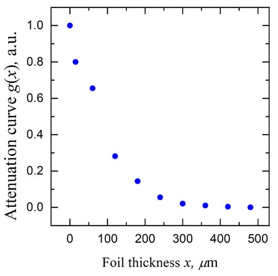
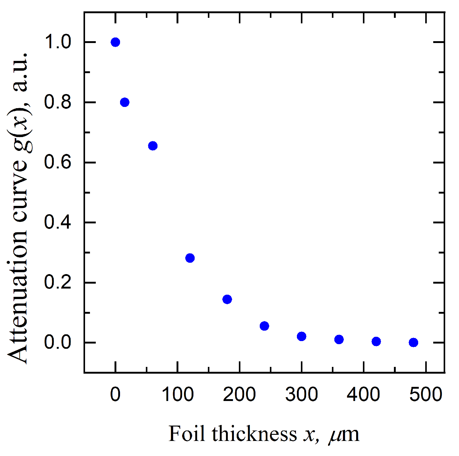
For the specified gas-diode configuration, a set of attenuation-curve data points was obtained, as shown in Figure 2. In [7], the reconstruction of the energy spectrum from the attenuation curve in Figure 2 was performed as follows. The amplitude-normalized attenuation curve dataset g(x) was expanded using spline interpolation from 10 measured points (Figure 2) to 80–100 points uniformly distributed over the interval x = [x_min, x_max]. The electron energy range ε = [0.05 MeV, 0.5 MeV] was likewise uniformly discretized into 50–100 grid nodes. Subsequently, a grid-based numerical solution of the Tikhonov regularization Equation (3) was carried out, yielding the reconstructed energy spectrum f(ε).

Figure 2. The experimental points of an attenuation curve for the high-pressure gas discharge in a diode with the spherical cathode [7].

It is important to note that (3) required the imposition of zero Neumann boundary conditions at the endpoints of the energy interval, i.e., f′(ε) = 0. The value of the regularization parameter was gradually decreased in order to improve the fidelity of the reconstructed distribution f(ε), provided that the solution of the regularized equation remained non-negative, thereby preserving the physical admissibility of f(ε). Further reduction of the regularization parameter increased the formal accuracy of the spectral representation. Still, it led to the growth of negative artifacts in f(ε), resulting in the loss of physical consistency of the reconstructed function.

To obtain the energy spectrum using the deep-learning approach proposed here (5), the λ₂ parameter was selected so as to constrain the maximum approximation error of the kernel K(x, ε) (6) to 10%. The λ₁ parameter was then varied systematically in order to cover several classes of relative accuracy of the attenuation-curve data (from a few percent down to the tenth of a percent). It is important to emphasize that the neural networks were trained directly on the original experimental dataset (Figure 2), without any additional preprocessing or artificial expansion of the attenuation-curve values via interpolation methods.

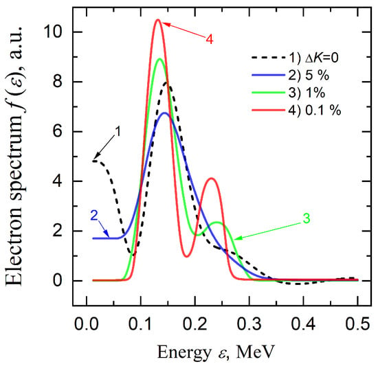
Figure 3 shows the energy spectrum reconstructions obtained with the deep-learning method (colored curves 2–4); for comparison, the energy spectrum previously obtained by solving the Tikhonov regularization Equation (3) is plotted as the black curve 1. As noted in [7], the Arsenin–Tikhonov method (3) revealed the principal maximum of the energy spectrum, corresponding to the main electron population, and a tail of the distribution extending up to 350 keV, indicative of anomalously high-energy electrons in the discharge. The data support this conclusion; however, it should be emphasized that curve 1 also displays two artifacts with no physical explanation: a spurious secondary maximum in the low-energy region at 12.5 keV and a negative excursion of the curve near 400 keV.

Figure 3. Reconstructed energy spectrum of fast electrons behind the anode: 1—solution of the incomplete inverse ill-posed problem (ΔK = 0); 2, 3, 4—solutions of the full inverse problem obtained using the proposed deep-learning approach.

The solution of the full ill-posed inverse problem for Equation (1), with a sequential increase in the assumed accuracy of the attenuation curve (curves 2 and 3), not only confirms the physically justified conclusions of [7], but also refines them. In particular, it resolves not only the principal maximum of the energy spectrum but also a secondary maximum corresponding to a population of runaway electrons with anomalously high energies. At the same time, the reconstructed spectrum remains strictly non-negative over the entire investigated energy range. Curve 4 represents a predictive distribution of electrons over energy for a scenario in which the possible relative experimental uncertainty is reduced to “optimistic” values on the order of 0.1%. The comparison of curves 2–4 illustrates a consistent trend toward the recovery of a nontrivial two-peak structure of the energy spectrum, while explicitly accounting for uncertainties present both in the attenuation curve and in the Tabata-Ito Formula (6).

3.2. Electron Beam from a Subnanosecond Pulsed Vacuum Discharge

As a second example, we used an attenuation-curve dataset g(x) for an electron beam at the exit of a vacuum diode [6]. The objective of this study was likewise to identify a nontrivial structure in the electron energy spectrum, specifically the presence of a fraction of electrons with anomalously high energies, ε > qU_max.

In experiments [6] aimed at determining the energy spectrum of a nanosecond electron beam generated by a vacuum diode driven by voltage pulses from the compact RADAN-220 generator (characteristic impedance 20 Ω, pulse amplitude 250 kV, and full width at half maximum 2 ns), an IMA3-150E electron tube with a beryllium-foil output window was employed. The tube featured a tubular cathode and a planar anode configuration. To ensure controlled beam conditions, the electron beam was collimated using a copper diaphragm with a 5 mm aperture, limiting the divergence angle of the main electron fraction to no more than 10 degrees. Beam current and charge measurements were performed using two types of diagnostics: a shunt based on chip resistors (2.7 Ω) and a collector sensor built on a 50 Ω coaxial line. Both diagnostics provided a temporal resolution of approximately 0.1 ns, and their signals were recorded using a TDS6604 digital real-time oscilloscope (6 GHz bandwidth). A more detailed description of the experimental setup and instrumentation is given in [6].

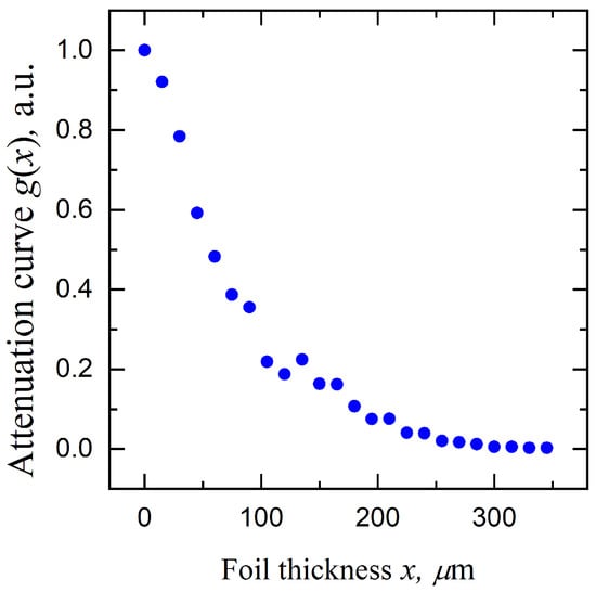
To construct the attenuation curves g(x), the beam was passed through a set of aluminum foils with a total thickness of up to 345 μm (15 μm increments). The experimental dataset (24 points) of the normalized attenuation curve is presented in Figure 4.

Figure 4. The experimental points of an attenuation curve for the pulsed subnanosecond vacuum discharge [6].

In [6], the experimental attenuation-curve dataset g(x) was processed using a spectrum-reconstruction technique analogous to that of [7]. This method involved first preprocessing the data from Figure 4 through interpolation, followed by solving (3) on the resulting uniform grid. The criterion for achieving maximum reconstruction accuracy was likewise the requirement that the reconstructed function f(ε) remain non-negative over the entire range of investigated energies.

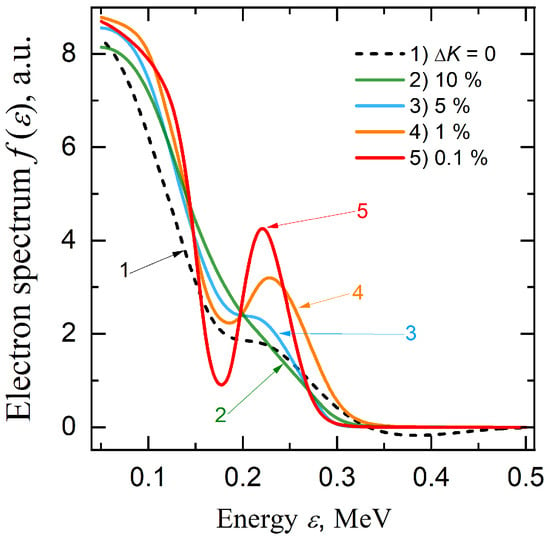
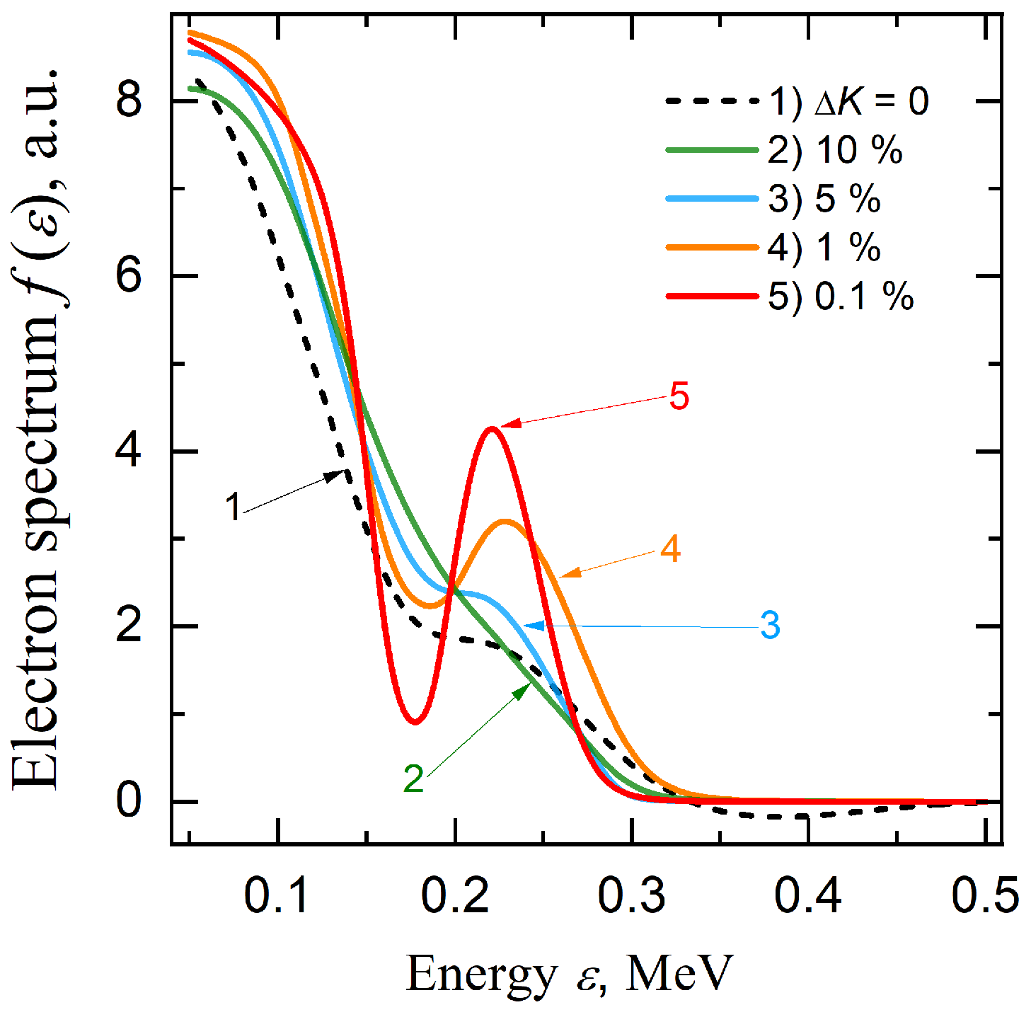
Figure 5 presents the reconstructed energy spectra obtained using the deep-learning method (colored curves 2–5); for comparison, the energy spectrum previously obtained by solving the Tikhonov regularization Equation (3) from [6] is shown as the black curve 1. The Arsenin–Tikhonov method (3) similarly revealed (curve 1) an anomalous plateau in the energy spectrum, localized between 200 and 320 keV, indirectly indicating the presence of electrons with anomalously high energies in the pulsed vacuum discharge. As in Section 3.1, a small negative excursion of curve 1 is also observed near 370 keV. This curve represents the most precise result of the Arsenin–Tikhonov method (3).

Figure 5. Reconstructed energy spectrum of electrons behind the anode: 1—solution of the incomplete ill-posed problem (ΔK = 0); 2–5—solutions of the full inverse problem obtained using the proposed deep-learning method.

In Figure 5, the colored curves represent energy spectra reconstructed at different values of the regularization parameter λ₁, corresponding to specified relative errors of the attenuation curve when the regularizing term of the full functional (4) is included. For a relative error not exceeding 10% (curve 2), the reconstructed spectrum is relatively coarse and does not exhibit additional regions of enhanced electron density. But at a 5% error level (curve 3), a feature begins to emerge in the energy spectrum resembling the plateau observed previously (curve 1). Further increasing the reconstruction accuracy (curve 4) highlights a secondary maximum corresponding to the population of electrons with anomalously high energies. An “optimistic” forecast (curve 5, corresponding to a 0.1% error level) clearly resolves the two-peak structure of the energy distribution. In all cases of the full problem solution (curves 2–5), the distribution function f(ε) remains strictly non-negative.

The quantitative validity of the reconstructed spectra is further confirmed by the low root-mean-square error (RMSE) of the calculated attenuation curves, which remained below the experimental uncertainty level (2–5%) in all presented cases. The transition from a plateau to a clearly resolved secondary peak (Figure 3 and Figure 5) in the region of 220–230 keV, extending up to 350 keV. According to the reflection of a statistically significant trend that also aligns with the “anomalous electron” theory, i.e., [11], it is uncovered that only a small portion of electrons become “anomalous”.

4. Conclusions

This article develops and implements a deep learning-based methodology for restoring energy spectra, which effectively solves the ill-posed inverse problem for the Fredholm equation of the first kind (1), while taking into account measurement errors in both the attenuation curve input data and the kernel of the integral operator (2). Solving the complete problem within the proposed methodology has the following advantages:

• The method is meshless and does not require any modification of experimental data sets before processing, i.e., it works directly with “raw” experimental data, which, for example, eliminates sampling errors and the influence of interpolation artifacts on the final result;
• The application of this approach resolves the issue of the influence of inaccuracies in the kernel of the integral operator of the equation K(x, ε), the magnitude of which can significantly exceed the magnitude of errors in the attenuation curve g(x);
• Although this approach introduces an additional source of error into Equation (1)—ΔK ≠ 0, correct processing of experimental data allows us to resolve non-trivial features of the reconstructed energy spectrum (secondary maxima in the high-energy region), which in Tikhonov’s method were only reflected as a plateau or masked by numerical noise;
• Even with sparse sets of real experimental data, the method has great predictive potential, allowing us to predict subtle features of the energy spectrum structure that may become observable with further improvements in measurement accuracy.

In general, the proposed methodology serves as a robust and reliable tool for solving full inverse problems in pulsed power and accelerator physics, particularly when dealing with sparse and noisy experimental datasets. Taking into account experimental inaccuracies in the kernel of the integral operator opens up some prospects for predicting the transformation of reconstructed energy spectra while increasing the accuracy of the measured input data sets.

References

- Mesyats, G.A. Pulsed Power; Springer: Berlin/Heidelberg, Germany, 2005; 568p. [Google Scholar]
- Bugaev, S.P.; Koshelev, V.I.; Timofeev, M.N. Electron-energy spectrum in high-current vacuum diode. Zh. Tekh. Fiz. 1974, 44, 1917–1921. [Google Scholar]
- Baksht, E.H.; Kostyrya, I.D.; Lipatov, E.I.; Lomaev, M.I.; Rybka, D.V.; Tarasenko, V.F. Excess-energy electrons in a nanosecond electron beam from a vacuum diode. Zh. Tekh. Fiz. 2007, 77, 98–103. [Google Scholar] [CrossRef] [Scilit]
- Tarasenko, V.F.; Baksht, E.K.; Burachenko, A.G.; Kostyrya, I.D.; Lomaev, M.I.; Petin, V.K.; Rybka, D.V.; Shlyakhtun, S.V. Energy distribution of runaway electrons generated by a nanosecond discharge in atmospheric-pressure air. Plasma Phys. Rep. 2008, 34, 1028–1036. [Google Scholar] [CrossRef] [Scilit]
- Tikhonov, A.N.; Arsenin, V.I. Solutions of Ill-Posed Problems; Winston & Sons: Washington, DC, USA; New York, NY, USA, 1977; 258p. [Google Scholar]
- Kozyrev, A.V.; Kozhevnikov, V.Y.; Baksht, E.K.; Buranchenko, A.G.; Tarasenko, V.F. Spectrum reconstruction of a nanosecond electron beam from the data on its extinction in thin foils. Russ. Phys. J. 2010, 53, 361–368. [Google Scholar] [CrossRef] [Scilit]
- Baksht, E.H.; Burachenko, A.G.; Kozhevnikov, V.Y.; Kozyrev, A.V.; Kostyrya, I.D.; Tarasenko, V.F. Spectrum of fast electrons in a subnanosecond breakdown of air-filled diodes at atmospheric pressure. J. Phys. D Appl. Phys. 2010, 43, 305201. [Google Scholar] [CrossRef] [Scilit]
- Kozyrev, A.V.; Kozhevnikov, V.Y.; Vorobyov, M.S.; Baksht, E.K.; Burachenko, A.G.; Koval, N.N.; Tarasenko, V.F. Reconstruction of electron beam energy spectra for vacuum and gas diodes. Laser Part. Beams 2015, 33, 183–192. [Google Scholar] [CrossRef] [Scilit]
- Kozyrev, A.; Kozhevnikov, V.; Semeniuk, N. Why Do Electrons with “Anomalous Energies” appear in High-Pressure Gas Discharges? EPJ Web Conf. 2018, 167, 01005. [Google Scholar] [CrossRef] [Scilit]
- Zubarev, N.M.; Kozhevnikov, V.Y.; Kozyrev, A.; Mesyats, G.A.; Semeniuk, N.S.; Sharypov, K.; Shunailov, S.A.; Yalandin, M.I. Mechanism and dynamics of picosecond radial breakdown of a gas-filled coaxial line. Plasma Sources Sci. Technol. 2020, 29, 125008. [Google Scholar] [CrossRef] [Scilit]
- Kozhevnikov, V.Y.; Kozyrev, A.V. On the Physical Nature of “Anomalous” High Energy Electrons in Vacuum Diodes. Russ. Phys. J. 2022, 64, 2341–2349. [Google Scholar] [CrossRef] [Scilit]
- Tabata, T.; Ito, R. A generalized empirical equation for the transmission coefficient of electrons. Nucl. Instrum. Methods 1975, 127, 429–434. [Google Scholar] [CrossRef] [Scilit]
Disclaimer/Publisher’s Note: The statements, opinions and data contained in all publications are solely those of the individual author(s) and contributor(s) and not of MDPI and/or the editor(s). MDPI and/or the editor(s) disclaim responsibility for any injury to people or property resulting from any ideas, methods, instructions or products referred to in the content. |
© 2026 by the authors. Licensee MDPI, Basel, Switzerland. This article is an open access article distributed under the terms and conditions of the Creative Commons Attribution (CC BY) license.