


Abstract
Spatially resolved absolute intensities of the atomic lines , , , and have been measured and analyzed in pure hydrogen plasma in the linear plasma device PSI-2. Two regimes have been investigated, with nominal (0.04 Pa) and elevated (0.5 Pa) gas pressure in the sample chamber. The measurements have been compared with local 0D calculations taking into account radiation from , , and channels. A baseline plasma chemical mechanism developed in magnetic fusion research was applied to calculate the density. Both the plasma chemical mechanism and the population factors applied are based on Sawada–Fujimoto collision-radiative model of atomic and molecular hydrogen. The calculations were found to reproduce both the absolute radiation and the line radiation intensity ratios measured in the 0.04 Pa experiment with electron temperature = 2–10 eV and electron density ∼5 × 10¹⁷ m−3. An exception is the intensity ratio, which tends to be overestimated by the model. The calculations suggest that the majority of the observed Balmer radiation in this regime is due to the channel. At the same time, both the applied simplified approach without detailed transport modeling and the baseline mechanism were found to be inappropriate for the 0.5 Pa experiment with reduced = 1–5 eV. This experimental regime can serve as a benchmark of more sophisticated hydrogen plasma models.
1. Introduction
Understanding the chemical kinetics of hydrogen plasmas is crucial for a number of important applications such as film deposition [1,2], ion sources [3], and boundary plasma of magnetic fusion reactors [4]. A type of experiment which enables detailed investigation of the hydrogen plasma chemistry is linear plasma devices (LPDs) [5]. Magnetized cylindrically shaped low-temperature plasmas with high degree of ionization generated in LPD provide convenient diagnostic access, a wide variety of operational conditions, and are well suited for validation of computational models.
Molecular processes produce excited atoms in specific electronic states [6], which manifest themselves in both the absolute intensities of line radiation and in the distribution over individual lines [7,8]. This effect is the basis of the Balmer lines analysis of hydrogen plasma chemistry, which is known in magnetic fusion research and has been applied in various fusion-related LPD experiments, such as PISCES-A [9,10], NAGDIS-II [11,12], GAMMA 10 [13], and Magnum-PSI [14].
The subject of the present paper is the application of the Balmer lines intensity measurements in LPD PSI-2 as a benchmark of plasma chemical mechanisms. PSI-2 [15] is a device with a hot cathode arc source of a type similar to PISCES-A. This experiment is equipped with a number of spectroscopic tools applied as diagnostics of plasma and plasma–wall interactions [16,17,18,19,20,21]. In the present work, an imaging spectrometer was utilized to measure the spatially resolved intensities of lines , , , and . Two operational regimes of the pure hydrogen discharges are investigated. The first one is without extra gas puff in the sample chamber and with nominal gas pressure there; the second one is with gas puff and with elevated pressure. The Balmer radiation measured in the two regimes differs substantially in terms of the absolute intensity, but most significantly in terms of the line intensity ratios.
The measurements are evaluated by comparing them with local 0D calculations. The model input is provided by the movable Langmuir probe and pressure gauge. The plasma chemical mechanism ‘ITER 2005’ [22,23] widely used in magnetic fusion research [24,25] was taken as the baseline model. It has been found that in the nominal pressure case, the measurements can be described quantitatively by this baseline plasma chemistry and without sophisticated transport modeling. The analysis suggests that the channel is the dominant source of the observed Balmer radiation. However, the model applied clearly failed to reproduce the measurements at elevated pressure. The reasons of that are both the limitations of the plasma chemical mechanism and the transport effects not included in the calculations. The experiment with extra gas puff can, thus, serve as a future benchmark for more detailed models of the hydrogen plasma chemistry and transport, including vibrational kinetics and radiation opacity. At the same time, the nominal pressure result can be seen as partial validation of the mechanism ‘ITER 2005’ for a certain range of parameters.
The simplified method of the present paper allows for only preliminary evaluation of the experiment in question. Besides the ‘first order approximation’ modeling approach, the main shortcoming of the applied plasma chemical mechanism is that it does not include detailed vibrational kinetics of and . Measuring the atomic Balmer radiation alone would be not sufficient for benchmarking of a model with detailed vibrational kinetics. In that case, in addition to Balmer lines, the analysis of the molecular Fulcher band radiation will be mandatory.
The rest of the paper is organized as follows. Section 2 describes the experimental setup and the measurement results. Section 3 provides a description of the theoretical model. This includes a brief discussion of the excitation channels of atomic radiation and calculation of the densities of the participating species , , . Section 4 describes the results for the nominal pressure case: comparison with the experiment (Section 4.1), verification of the model assumptions (Section 4.2), and model predictions not directly accessible to the measurements, such as the concentration of (Section 4.3). The following Section 5 addresses the case with elevated pressure. Lastly, Section 6 summarizes the main findings.
2. Description of the Experiment
2.1. Experimental Setup and Diagnostics
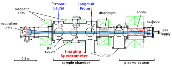
PSI-2 is a linear plasma device where plasma is generated by arc discharge between a heated LaB6 cathode and hollow molybdenum anode. The plasma is confined by an axial magnetic field of strength around 0.1 T. In the sample (exposure) chamber where the measurements take place (Figure 1), the magnetic field is nearly homogeneous. The sample chamber is separated from the source chamber by a diaphragm; each chamber has its own pumps. This setup enables separate gas pressure control in the plasma source and in the sample chamber. More information about the PSI-2 device can be found in [15] and references therein. In the experiments which will be considered here, the sample target was removed and the plasma was only limited by the neutralizer plate. The electric current of the plasma source was set to 100 A (discharge power 7 kW); the source is fed by gas puff 100 sccm.
Figure 1.
Scheme of the PSI-2 experiment and diagnostics.
The diagnostics used for the experiments in question are the pressure gauge, movable (reciprocating) Langmuir probe, and imaging spectrometer (Figure 1). The pressure gauge is the Pfeiffer PKR 251 combined Pirani/cold-cathode transmitter. The expected measurement error according to the manufacturer is ±30% [26]. The Langmuir probe provides radially resolved electron temperature and density . The reconstruction of the plasma parameters from the measured voltage–current characteristics is not always straightforward [27], especially in magnetized plasma [28], and the systematic uncertainty of the probe data can be large, but exact error bars are difficult to estimate. For the subsequent analysis, relative error ±25% will be assigned to , and ±50% to . Those values are larger than statistical variations between spatially close points (see Supplementary Materials).
For the spectroscopic measurements, the same hardware and experimental layout as in [19,20] is used: imaging spectrometer ARC (Acton Research Corporation) SpectraPro-750; the light is transmitted to the entrance slit via quartz observation window and through the air. The images are taken over cross-section perpendicular to the plasma axis. Typical exposure times are 5–10 s. The camera has a spatial resolution of 400 pixels corresponding to 10 cm of physical length. The spectra are resolved on 1600 pixels, which cover a wavelength range of approximately 20 nm. The measurements were absolutely calibrated by integrating sphere USS600 with known spectral radiance, cross-checked against lab-sphere USS1200. Measurements of the and lines were performed with a gray filter to prevent integer overflow of the camera’s storage.
For the subsequent analysis, absolute radiation intensities of spectral lines integrated over wavelength are required. The spectral resolution of the spectrometer and camera applied, although relatively low, was found to be fully sufficient to isolate the individual atomic hydrogen lines and to perform the integration. The procedure of calculating the integral S with background separation, and estimate of the uncertainty of this procedure (‘integration error’), is outlined in Appendix A. The ‘background’ nearly uniformly distributed over wavelengths is thought to include both continuum radiation from the plasma and stray light dispersed after multiple diffuse reflections. Only the lines of sights for which % are selected for comparison with calculations and to appear on the plots.
The absolute radiation intensities I are obtained by multiplying the values S found by the procedure of Appendix A with the calibration factors c. The total error of is the sum of the error of integration and the error of calibration . The uncertainty of the calibration factor is caused by, first, the spatial inhomogeneity of the calibration signals and the difference between repeated calibration measurements. Second, the noise and signal to noise ratios of the calibration signals. The calibration error is increased for lower wavelengths, and for lines other than , the dominant term in is . It should be emphasized that c and are the same for all lines of sight, and is also not entirely uncorrelated between the lines of sight because this is partly an algorithmic uncertainty. Therefore, all error bars of the experimental radiation intensities on the plots below show mainly systematic error not correlated between spatial points. They can be interpreted as the range within which the whole experimental profile may be shifted upward/downward roughly preserving its shape.
In the present experimental setup, the Langmuir probe is positioned approximately 40 cm upstream from the location of the spectroscopic measurements. This inconsistency may introduce extra uncertainty into the data evaluation. The analysis of this work is based on the assumption that , are uniform along the field lines. This assumption is supported by 2D transport modeling of PSI-1 and PSI-2 plasma [29]. Certain experimental evidence is provided by the spectroscopic measurements performed in PSI-2 at two different axial positions reported in [20]. For , they show, indeed, less than a 20% difference between two locations at gas pressure 0.7 Pa, but the difference increases with increased pressure and can reach almost a factor of 2 at 1.1 Pa. For , only measurements at high pressures are available, and only for the recombining zone where < 1 eV. They indicate a very large—much more than a factor of 2—axial difference, but apparently not representative for all radial positions and for lower gas pressure. To conclude, for , the possible reduction from upstream to downstream positions detected experimentally is effectively included into the error bar ±50% assigned above. For , there is no reliable experimental evidence of the magnitude of the axial variation, although there are numerical simulations which suggest that at least at not too high gas pressure this variation is weak.
2.2. Results of the Measurements
Two experimental regimes with pure hydrogen plasma were investigated. The first is the reference experiment without gas puff in the sample chamber and with nominal gas pressure there, named here ‘0.02 Pa case’. The second is an experiment with extra gas puff 80 sccm and elevated pressure, named ‘1 Pa case’. The pressure values referred to above are readings of the pressure gauge. They must be translated into real pressure, which depends on the gas composition [26]. Subsequently, ‘0.02 Pa’ here corresponds for to real pressure 0.04 Pa, and ‘1 Pa’ corresponds to 0.5 Pa. The pressure gauge readings rather than real pressure are used as designation of the experimental cases throughout the paper to conform to the naming convention in the experimental notebooks.
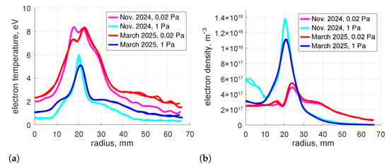
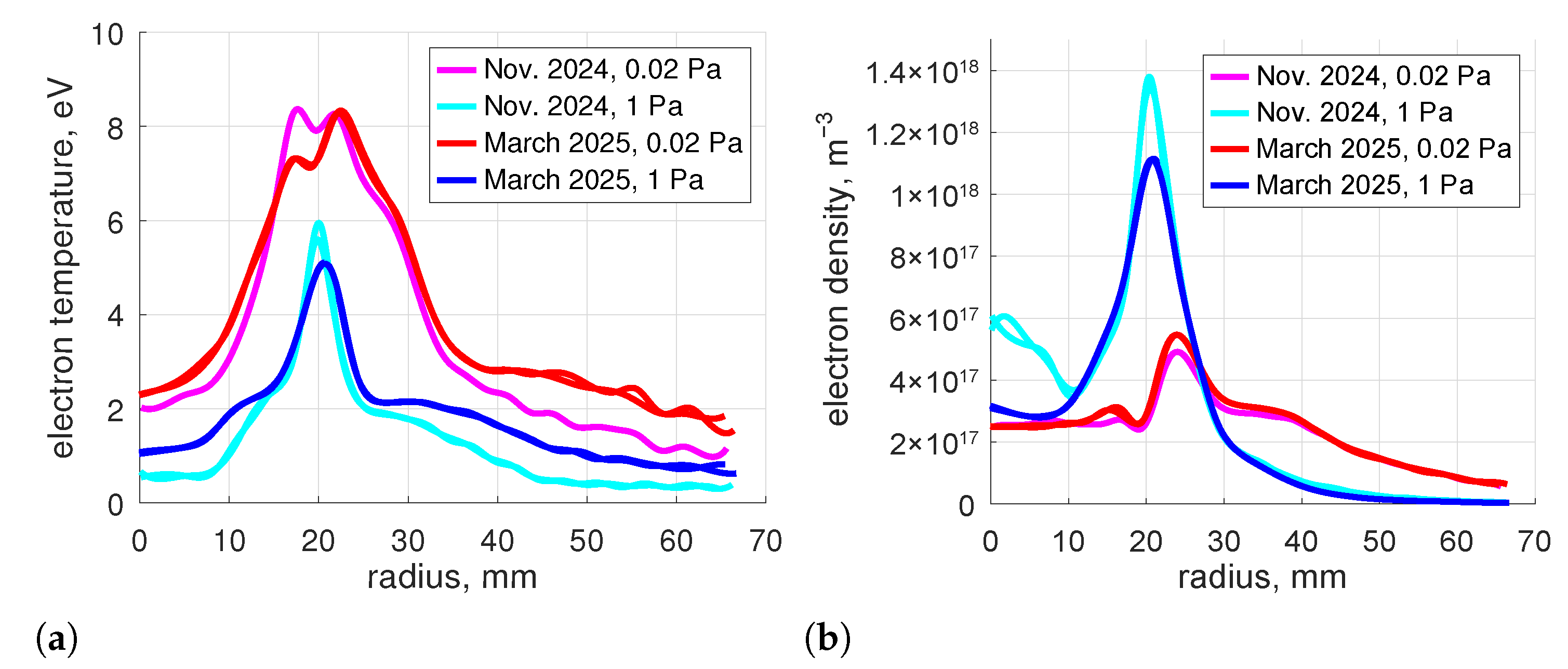
Two series of experiments with identical settings were performed in November 2024 and in March 2025. Scheduled maintenance took place between those two sets of measurements during which, in particular, the LaB6 cathode of the plasma source was replaced. The plasma parameters obtained in both series are presented in Figure 2. Two Langmuir probe runs are performed for each plasma regime, before and after the spectroscopic measurements. The results are nearly identical, both shown in Figure 2. The profiles shown are piecewise least square cubic spline fits of radially resolved , taken from the processed Langmuir probe data. One can see good reproducibility of the plasma parameters in two independent campaigns and a clear difference between the nominal pressure and the elevated pressure regimes. The characteristic profiles with maxima around 2 cm from the axis occur as a results of the hollow cathode design of the plasma source [15].
Figure 2.
Plasma parameters. Piecewise least square cubic spline fits of the processed Langmuir probe data.
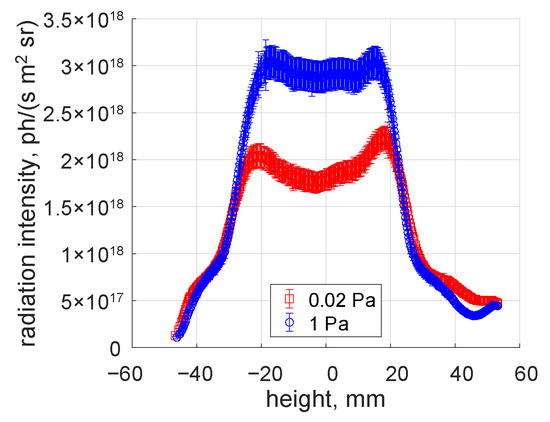
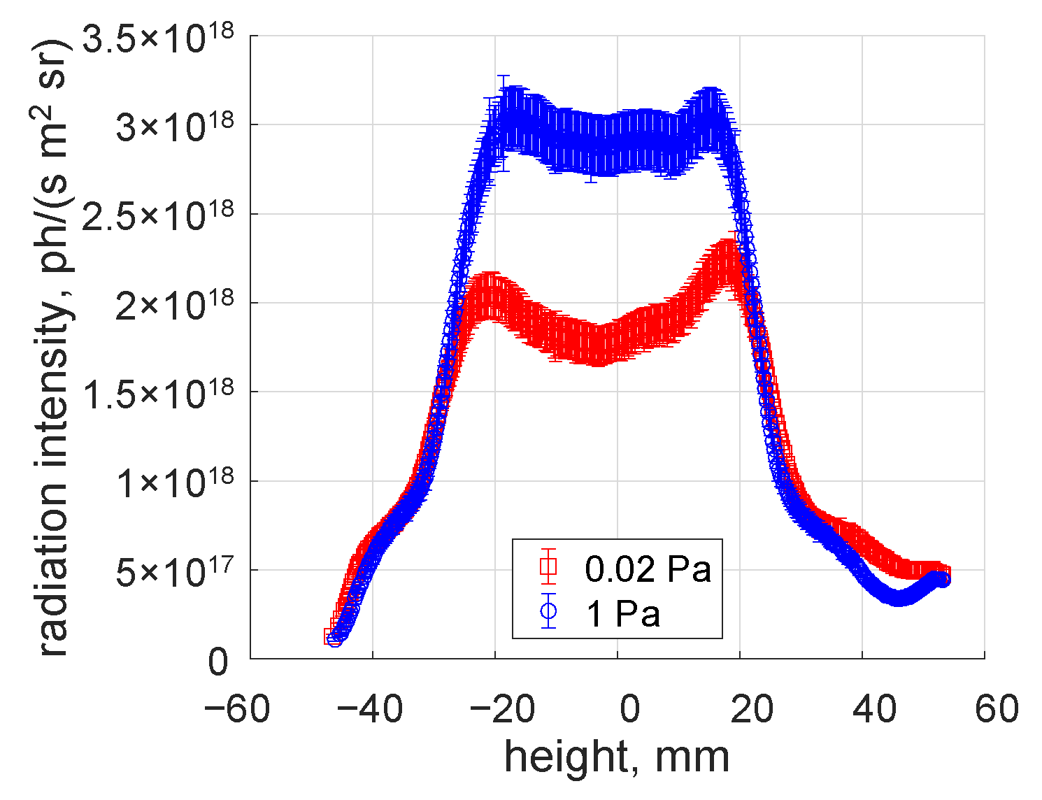
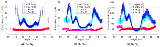
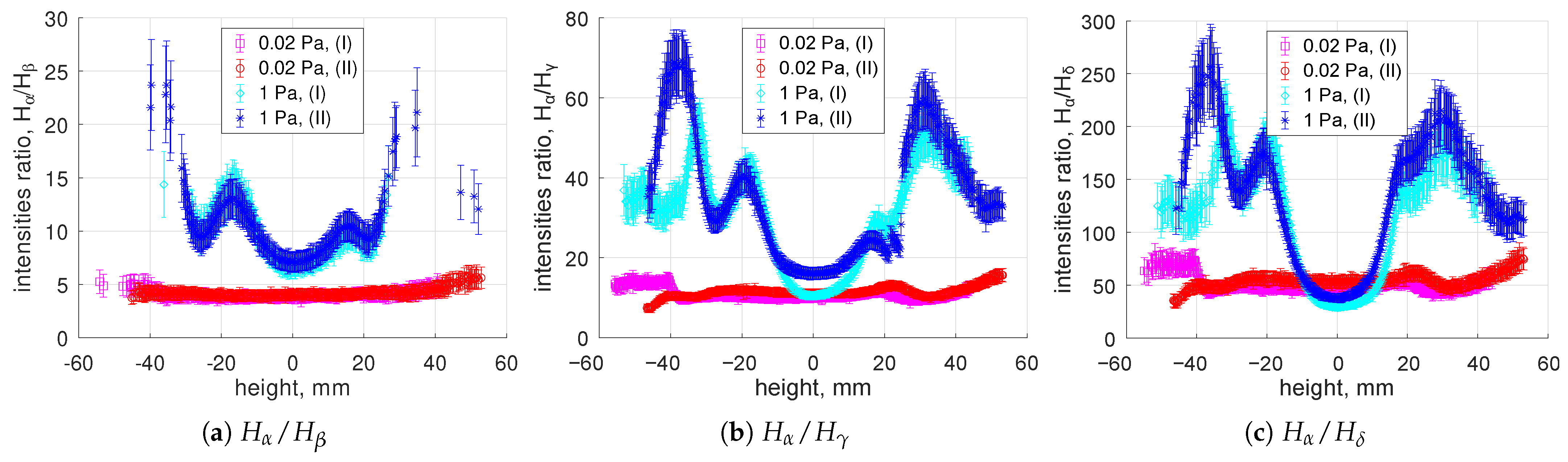
In all conditions studied, lines , , , and were always found to be bright enough to be detected over the background, and their acquired profiles are clean enough for integrals over wavelengths to be calculated. In the 1 Pa case, this applies to as well. The obtained absolute intensities of radiation and the line intensity ratios are shown in Figure 3 and Figure 4 respectively. The error bars for the ratios are calculated on assumption that the errors of intensities of different lines are uncorrelated. As one can see in Figure 4, the ratios obtained in both series are reproduced very well. The difference between the 0.02 Pa and 1 Pa experiments is apparent and by far exceeds the error bars. This applies to the absolute intensities (Figure 3), but especially to the intensity ratios (Figure 4). For those latter the difference between the two regimes also clearly by far exceeds the variation between the two series of measurements.
Figure 3.
Absolute intensity of radiation. The error bars show mainly systematic uncertainty; see the comment in Section 2.
Figure 4.
Line radiation intensity ratios. (I) is the ‘November 2024’ series of measurements; (II) is ‘March 2025’. The error bars show mainly systematic uncertainty; see the comment in Section 2.
Only the absolute intensity of the ‘March 2025’ series is shown in Figure 3. The absolute values obtained in ‘November 2024’ appeared to be by approximately a factor of 1.5 lower, but as the most likely reason of this discrepancy inconsistencies found later in the calibration for the ‘November 2024’ experiment were identified. In the comparison of the experiment and calculations below, only measurements of the ‘March 2025’ series will be used.
Figure 3 and Figure 4 suggest that the plasma in those experiments can be only approximately considered as cylindrically symmetric. The main reason of the asymmetry is non-uniformity of the plasma source. The symmetry was seemingly improved somewhat after the cathode renewal, which is one more reason why only the ‘March 2025’ series is considered in the following analysis. Subsequently, the position of the plasma center on the spectrometer images cannot be defined precisely. The zero of the coordinate ‘height’ set here on all plots is determined approximately from the and intensity profiles obtained in 1 Pa case. They appear nearly symmetric and have a clear maximum to which the position of the plasma axis can be ascribed.
3. Description of the Model
3.1. Excitation Channels
The local volumetric photon sources are calculated as a sum of the contributions of individual excitation channels [8,30,31]:
where is the number density of the electronically excited atoms (here the letter n is used for both number densities and the principal quantum number of hydrogen atom, but the usage must be unambiguous from the context), is the Einstein coefficient of spontaneous emission, are the population factors of specific excitation channels [8], and are the number densities of the corresponding ground species. The factors are calculated by a collision-radiative model for hydrogen atoms in quasi-static approximation—that is, on assumption that the excited states are short-lived and their transport can be neglected. Also in all calculations here, optically thin gas is assumed. As it will be discussed later in Section 4.2, this assumption is valid for Balmer lines, but absorption of Lyman lines could start to become significant for the atom densities in question.
Three excitation channels are taken into account. stands for excited atoms produced by dissociation of molecules, reaction in Table 1; is the channel related to dissociative recombination and dissociation of molecular ion , with reactions , shown in Table 1; is the electron impact excitation of the ground state atoms. Excited atoms can be also produced by recombination of ions, but preliminary analysis has shown that this channel is negligible under the conditions in questions.
The population factors as well as all rate coefficients used in this work and listed in Table 1 (except ) are based on the collision-radiative model for atomic and molecular hydrogen developed by K Sawada and T Fujimoto [8,32] and extended by P Greenland and D Reiter [33]. They are taken from the data compilation AMJUEL [34] used for magnetic fusion applications. To complete the information of Table 1: , , are entries AMJUEL H.12 2.2.5, 2.2.14, 2.1.5 of [34] respectively. The coefficients used here include electronically excited states of but, with exception of , which otherwise would be extremely small, do not include vibrationally excited states.
The effective rate coefficient is obtained for quasi-static population of vibrational states of —that is, for the population of calculated by solving 0D balance equations taking into account electron impact vibrational excitation/de-excitation and destruction of in processes , , . The applicability of quasi-static approximation here is questionable, and cannot be verified within the present approach. This is a serious shortcoming of the applied set of rate coefficients which can lead to unreliable results especially at the plasma periphery where, as will be discussed in Section 4.3 below, production of is always dominated by . Another issue is related to the assumptions on vibrational distribution of . The rate coefficients of dissociative excitation and dissociative recombination of , in general, depend strongly on its initial vibrational state ; see e.g., [35] Sections 7.1.2, 3 there. Moreover, distribution of the dissociative recombination products over excited states is especially sensitive to ([35]; Section 7.1.3C). The AMJUEL rate coefficients , and the corresponding population factor of the channel are based on [6], processes 2.2.12, 2.2.13, 2.2.14 there. The rate coefficients of dissociative excitation 2.2.12, 2.2.13 in [6] represent the ‘average’ vibrational state . The rate coefficient of dissociative recombination, process 2.2.14 in [6], which is the main source of excited atoms in the channel, is averaged over ‘experimental’ vibrational distribution of formed by ionization (see [6], process 2.2.9). This latter assumption—on which used in the present work is based—can be especially compromised, again, at the locations where is not the dominant source of anymore.
Table 1.
List of reactions.
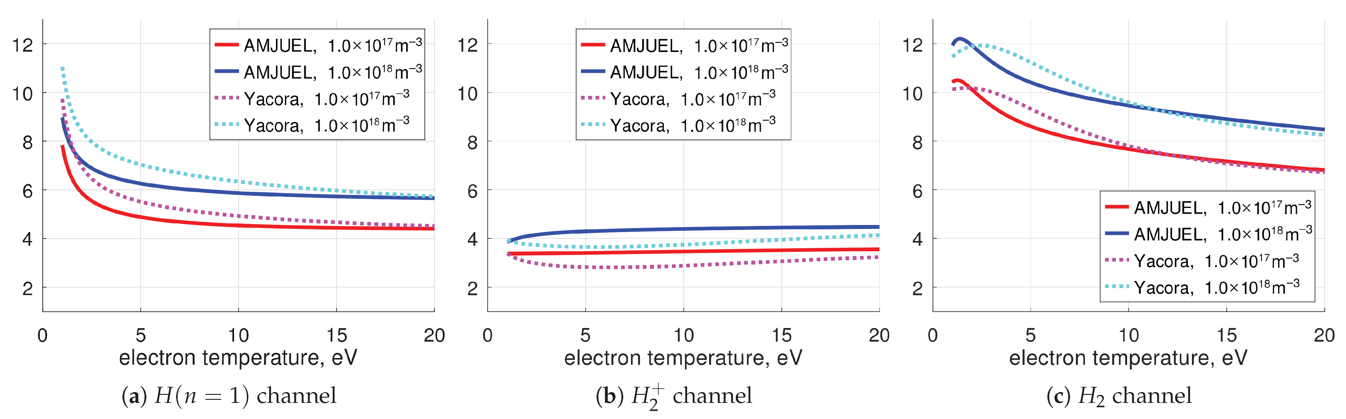
Atoms produced by different processes have specific population distributions of the electronically excited states, and their line radiation can be used as a spectroscopic signature of the individual excitation channels [7,8]. This effect is illustrated in Figure 5, which shows the radiation intensity ratios calculated theoretically for two Balmer lines. One can see that for < 10 eV, the difference in the ratios calculated for different channels is clearly larger than the variation with respect to plasma parameters. Figure 5 also presents comparison with another collision-radiative model, ‘Yacora on the Web’ [37,38]. Although there is no exact quantitative agreement between the two models, the results are very close.
Figure 5.
Theoretical line radiation intensity ratios for individual excitation channels; population factors from AMJUEL [34] are compared with ‘Yacora on the Web’ [37,38].
Comparing Figure 5 with the line intensity ratio measured experimentally in the 0.02 Pa case (Figure 4a) readily gives a clue that the majority of the Balmer radiation in this experiment is likely due to the channel. This simple consideration anticipates the results of a more detailed analysis based on Equation (1), which is presented below. The plasma parameters , required to apply (1) are taken from the Langmuir probe data. The task is then reduced to determining the densities , , . Their calculation will be explained in the subsequent sections. As one will see, the species densities are not entirely independent from each other. This weak non-linearity is treated in the computations by applying simple iterations.
In all model calculations described below, the plasma is assumed to be cylindrically symmetric. The wall is also approximated by a cylinder, and both the plasma and the wall are taken to be homogeneous and infinite in the axial direction. The model also involves a number of physics assumptions which will be verified afterwards (a posteriori) by examining the results of model calculations. It will be shown that they are largely valid for the 0.02 Pa case, but some of them are not justified for the 1 Pa case.
Excited atoms can be also produced by the and channels [30,31], which are not included in Equation (1) and are not taken into account in the present study. According to population factors of both AMJUEL and ‘Yacora on the Web’, even if the density of would be equal to , the contribution of the channel into Balmer radiation would be negligible. Nevertheless, the formation process (Table 1) can constitute a significant loss term of ions. Therefore, its effect on was estimated in a non-self-consistent way and will be discussed in the results sections below. Beyond that effect, the possible presence of can only have an indirect impact on the calculated radiation intensities: due to correction and due to a reduction in density and thus mitigation of the process (Section 3.3 below).
3.2. Calculation of Density
It is assumed that molecules are distributed uniformly in the sample chamber of the vacuum vessel, and their density is spatially constant there. Depletion due to interaction with plasma is neglected. It will be shown later in Section 4.2 by calculating the mean free paths of the corresponding inelastic and elastic collisions that this assumption is justified for 0.02 Pa, although it is less justified for the 1 Pa case (Section 5). The signal of the pressure gauge is proportional to the density of molecules inside the gauge , and this density is related to via the balance of incoming and outgoing fluxes. The gauge is connected with the vacuum vessel by a straight tube. Assuming that the vacuum transmission probability w of the tube is the same for particles coming from both directions, the flux balance at the gauge inlet can be written as:
Here is the flux of molecules per unit area through the inlet cross-section of the gauge towards the vessel, and is the effective molecular flux (per unit area) from the vessel to the entrance of the connecting tube. The first term of the sum is the fraction of that flux which reaches the gauge inlet; the second term is the fraction of the flux from the gauge which returns back due to collisions with the tube’s wall. The balance (2) is valid for free molecular flow inside the tube. Validity of this assumption is discussed in Section 4.2 and Section 5 as well. The flux is the sum of the flux of molecules and half of the flux of atoms. The first term is calculated on assumption that molecules are Maxwellian with translational temperature . The primary source of atoms in the system in question is molecular dissociation processes; therefore, the atomic flux should be proportional to . Then, the balance (2) can be written as:
where is the temperature inside the gauge (here = 300 K is always assumed), is the Boltzmann constant, and is the molecule mass. The coefficient of proportionality U is calculated below in Section 3.4 using Equations (11) and (12). Replacing in (3) by the pressure yields the final formula, which connects the measured pressure with :
To apply Equation (4), translational temperature must be known. For the discharges in question, no direct measurements of were available, and there is no strong evidence that can be significantly elevated over the room temperature 300 K. However, high 0.1 eV was reported earlier in PISCES-A [9], measured from the line width of hydrogen molecular lines. The molecule temperature can be increased due to the following processes: (i) elastic collisions with ions; (ii) rotational and vibrational excitation of by electron impact with subsequent rotational–translational (RT) and vibrational–translational (VT) relaxation; (iii) elastic collisions with atoms; and (iv) generation of hot molecules by surface recombination of atoms [39]. The process (i) is unlikely to be effective here because the free paths of such collisions are too long (Section 4.2; Table 2).
The electron impact excitation can be efficient, and rotational temperatures up to 600 K have been indeed measured in PSI-2 [20]. However, RT and VT relaxation proceeds via much slower collisions with heavy particles. The RT cross-sections for are more than 100 times smaller than gas kinetic cross-sections; see, e.g., [1] (Section 2.2.6). The probabilities of VT relaxation in + collisions for 1000 K are also small; see [40] (Chapter 7). Therefore, the process (ii) is also not expected to be efficient under the conditions in question. Nevertheless, elastic collisions between atoms and molecules (iii) could be efficient at elevated gas pressure; see Section 5 below and Table 2. The surface process (iv) also cannot be ruled out. In the calculations which are presented below, is treated as an uncertain parameter and is varied from 300 K to 1000 K.
3.3. Calculation of Density
The density of ions confined by the magnetic field is calculated in local 0D approximation on assumption that their transport is much slower than plasma chemical reactions. Validity of this assumption is not apparent and is discussed below in Section 4.2. Production and destruction of is modeled by the plasma chemical mechanism consisting of reactions , , , (Table 1). This mechanism, called ‘ITER 2005’, was developed by D Reiter et al. [22] on the basis of the Sawada–Fujimoto model [7,8]. It was introduced for the tokamak divertor modeling in [23] and is still widely applied in magnetic fusion research. The 0D balance equation reads:
Substituting the quasi-neutrality condition for plasma, , readily yields:
Equation (5) is applied at each radial position to obtain the spatial profile of . Technically, when , calculated by (5), is larger than , it is set to .
In the processed Langmuir probe data (Figure 2b), the electron density is calculated assuming that the plasma only consists of ions. For plasma, this value must be corrected. The sheath theory predicts that in weakly collisional multi-ion plasma, each ion species has at the sheath entrance approximately its single-ion sound speed [41,42]. Therefore, introducing the concentration , the ion saturation current can be written as:
where C is some constant, is ion temperature, and , are atomic masses of the corresponding ions. on the left-hand side is reconstructed from the electron density , which was calculated assuming : . Substituting this relation into (6) yields the equation, which translates from the processed Langmuir probe data to the corrected value :
3.4. Calculation of H-Atoms Density
The hydrogen atoms are divided into two groups. First are the atoms emerging after dissociation in the plasma volume, and the second are atoms re-emitted from the wall of the vacuum vessel. For the first group, it is assumed that their free paths are longer than the distance to the wall, and their density can be calculated assuming collisionless ballistic flow. Same as for for + collisions, one can show that this assumption is valid for the 0.02 Pa case, but is less valid for the 1 Pa case, as shown in Section 4.2 and Table 2 below. For atoms re-emitted from the walls, another assumption is applied: they are thermalized and distributed spatially uniformly inside the vessel.
The number density of the first group, ballistic atoms, is found by solving the collisionless flow problem for cylindrically symmetric isotropic single-speed particle source , where r is the radial coordinate. The semi-analytic solution of that problem is derived in Appendix B, Equation (A3). The total density is calculated as a sum of the contributions of the three strongest sources of H-atoms: reactions (in the order of importance) , , and in Table 1. The products’ kinetic energies required to calculate the absolute velocity u in (A3) are taken from [6]: 3 eV for , and 4.3 eV and 0.5 eV for and respectively.
The number density of atoms which do not recombine on the wall into molecules and are re-emitted back as atoms is found using the global balance (total source equals total sink):
where is the flux of the primary ballistic atoms incident to the wall, is the probability of surface recombination of H-atoms into molecules, and is the wall incident flux of the secondary—re-emitted—atoms. Both and are defined per unit axial length. The left-hand side of (8) expresses the global source of re-emitted atoms due to reflected ballistic atoms, and the right-hand side is their global sink rate. For thermal re-emitted atoms with spatially constant density , one can write:
where is the inner radius of the vacuum vessel, = 20 cm, is the temperature of atoms, and is their atomic mass. Substituting (9) into (8) yields the final formula:
Here, although for ballistic atoms ionization has been neglected, the ionization term is added for thermal atoms to make Equation (10) formally applicable for . is the ionization rate coefficient from Table 1.
The coefficient U in Equations (3) and (4), from Section 3.2 above, is calculated as the sum of the ballistic and thermal contributions :
where is same as with, in this case, minor contribution due to added for completeness; when performing calculations, this reaction is technically taken into account in in (1) as well.
, used in Equations (10) and (12), is estimated from the available experimental information. In high-resolution spectral measurements performed in discharges with similar plasma parameters in PISCES-A, it was found that the shape of the line can be described as a sum of two components, ‘cold’ and ‘hot’ [10]. The hot component rotates with plasma, and the cold component does not. This observation was confirmed in PSI-2 for the and lines [18,21]. The temperature of the unshifted cold component is thought to be representative for thermal atoms coming from the walls. The magnitude of this temperature found in both PISCES-A and PSI-2 is 0.25–0.5 eV [10,21]. In all calculations discussed below, the parameter is set to the lower value = 0.3 eV.
Whereas the uncertainty of appears to have a relatively weak impact on the calculated densities and fluxes of atoms, they depend strongly on another, also uncertain, parameter—the surface recombination coefficient . Experimental data for recombination of hydrogen on stainless steel are available in the literature, but their scattering is relatively large. The results of the older publications [43,44,45] can be summarized as = 0.1 ± 0.05. At the same time, in more recent works, larger values are reported: % in [46], in [47]. In [48], even —for steel with removed oxide. The outcomes of the measurements apparently depend on many factors, including the degree of oxidation and presence of impurities, along with the surface temperature and energy spectrum of incident atoms. For the calculations of the present work, is varied from 1 to 0.05, and the value is taken as the most probable reference.
4. Results for 0.02 Pa Case
4.1. Comparison of the Experiment with Model
To summarize, as the input for the calculations serve the , provided by the Langmuir probe, Figure 2, and the pressure measurement . For sensitivity assessment, is varied within ±50% of its reference value, within ±25%, and within ±30%. On all the plots in this section, the solid curves marked ‘ref.’ or ‘model ref.’ stand for calculations for the reference , , ; the dotted curves ‘min/max’ are, subsequently, the maximal and minimal value over the whole specified range of , , . Scans are made over parameters and . is varied from 300 K to 1000 K; is varied from 1 to 0.05.
The calculated local photon sources (emissivities) are compared with experimental ones obtained by Abel inversion of the measured radiation intensities (Figure 3 and Figure 4). The inversion is performed by least square minimization, which maps integrals over lines of sight into 14 radial positions. The number of positions is chosen as a compromise between radial resolution and accuracy—error bar—at each position. The latter are the transformed error bars of the radiation intensities; see Section 2.2. On the plots, experimental points with negative and with positive radii represent the result of the inversion applied to the intensity profiles, respectively, on the left and on the right from the plasma axis. Their difference is the uncertainty due to deviation of the plasma from exact cylindrical symmetry.
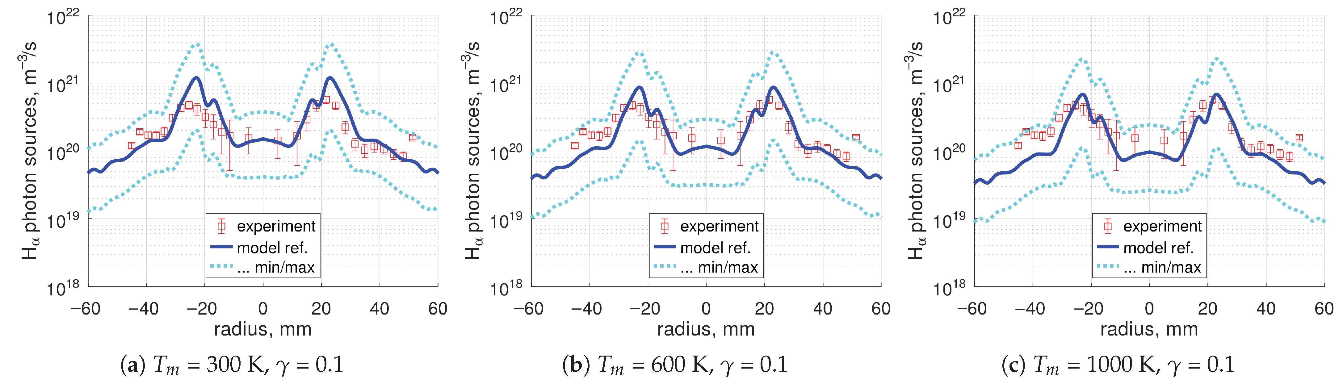
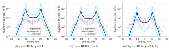
Comparison of the radial profiles of the absolute sources is presented in Figure 6. The dependence of the calculated signal on is weak (see Supplementary Materials)—thanks to feedback (4)—therefore, only scan over is shown. The dependence manifests itself as a rough proportionality to with very weak non-linearity. One can see in Figure 6 that the model can reproduce the experiment relatively well, both the shape of the radial profile and the absolute values. At the same time, the calculated signal is also seen to have very large, a factor of 3, variation with , , .
Figure 6.
The 0.02 Pa case, absolute photon sources, scan over .
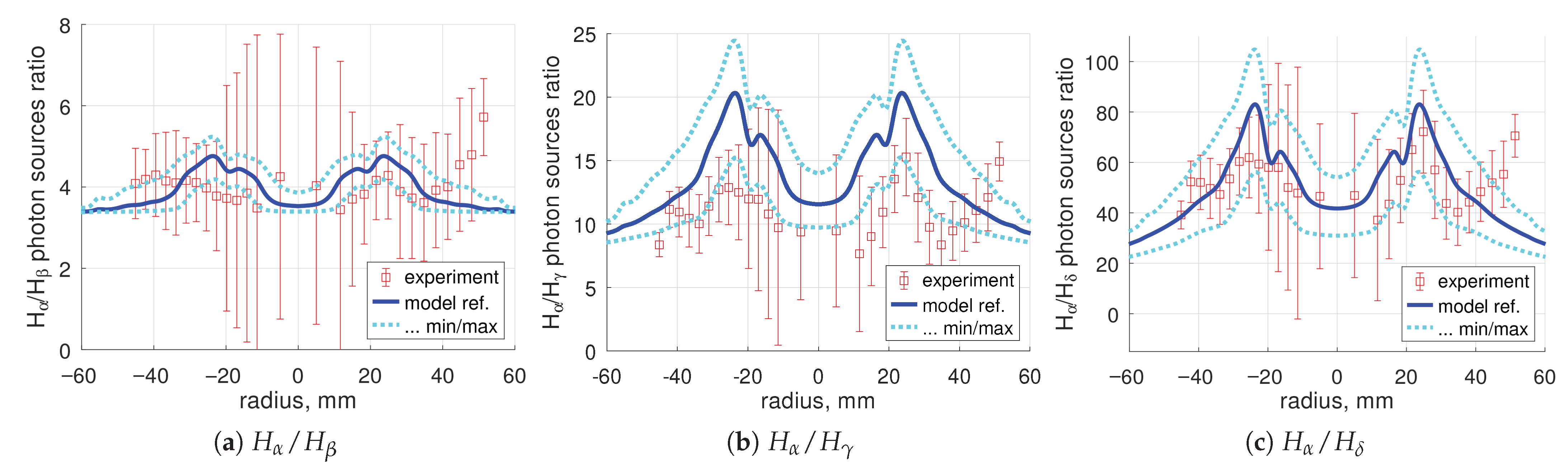
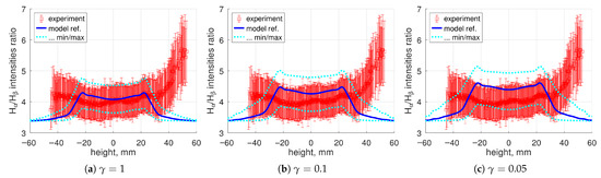
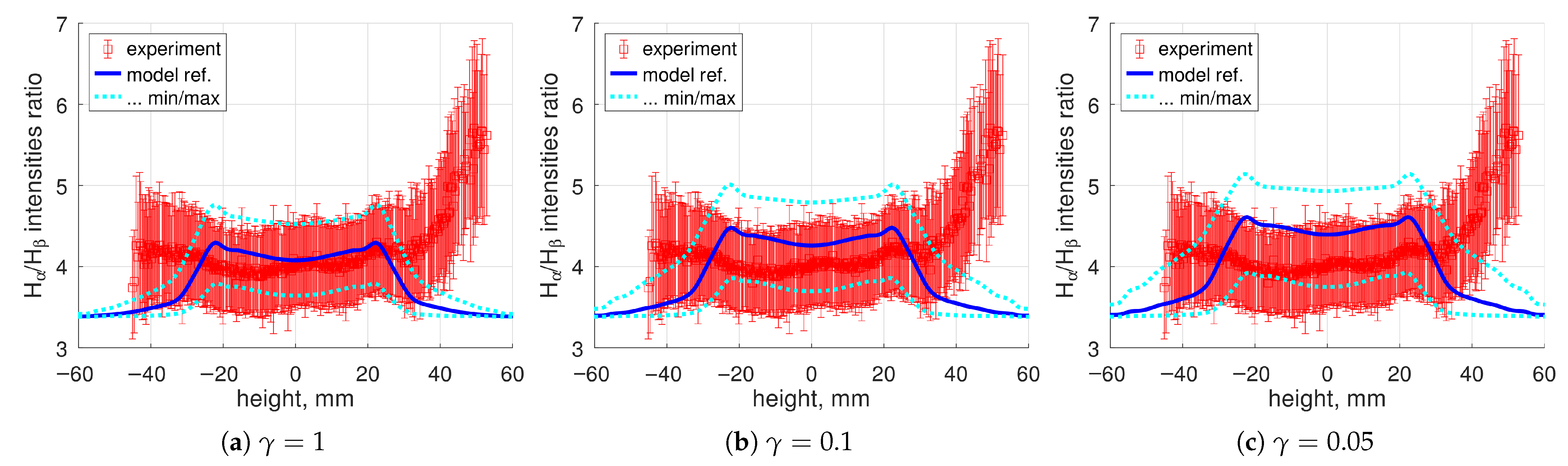
Ratios of the emissivities of individual lines are compared in Figure 7. They depend weakly on and (see Supplementary Materials); therefore, only one reference case is shown. The dependence on is best pronounced for the intensities (line of sight integrals) ratios; they are shown in addition in Figure 8. The calculated intensity ratio grows with decreased . The reason, as discussed in Section 4.3 below, is the increase in the share of the channel in the total radiation compared to the channel, which otherwise dominates. The channel leads to larger line intensity ratios than the channel (Figure 5). Best agreement is seen for .
Figure 7.
The 0.02 Pa case, lines emissivities ratios, = 0.1, = 300 K.
Figure 8.
The 0.02 Pa case, lines intensities ratio, scan over , = 300 K. The experimental error bars show mainly systematic uncertainty; see the comment in Section 2.
Both the absolute radiation (Figure 6) and the line emissivities ratios (Figure 7) obtained in the calculations are more peaked than in the experiment. Radiation profiles that are too peaked may be the result of neglecting the ion transport in the model. Strong maxima in the calculated emissivity profiles translate for the ratio of the line of sight integrated intensities into a top-hat profile with decaying lateral parts, whereas in the experiment, the radial distribution is much flatter. An example for can be seen in Figure 8.
The results observed for largely hold for as well (Figure 7c). However, for , (Figure 7b), the model tends to systematically overestimate the ratio, for the reference , by ≈50%. This discrepancy can be a consequence of the known inaccuracy of the excitation rates used in the old Sawada–Fujimoto model (see discussion in [30], Section 3.2). In addition, the disagreement suggests that a process which predominantly populates the level may be missing in the model. A possible candidate is the neutralization [49].
4.2. Verification of the Model Assumptions
To assess the importance of the collisions of neutral particles with plasma and gas, the mean free paths (MFPs) of the corresponding processes were calculated. They are provided in Table 2. The numbers in the table are minimum values taken over all spatial positions, over the whole range of the plasma parameters , , and the whole range of the parameters , , .
Table 2.
Estimated mean free paths of atoms and molecules.
Estimates of the ionization, , and charge–exchange, , MFPs of atoms are made for slower thermal atoms (shorter MFPs):
Here is the charge–exchange collision rate coefficient for atoms in electronic ground state taken from [6,36], process 3.1.8. In the denominator, is used instead of to provide a lower estimate. As one can see in Table 2, and are always an order of magnitude larger than the plasma diameter of ≈10 cm.
The MFPs of collisions with plasma are calculated as follows:
Here is MFP of inelastic collisions, with rate coefficients from Table 1 in the denominator; is MFP of elastic collisions with ions; is the rate coefficient of effective diffusion collisions [51] taken from [34], entry AMJUEL H.3 0.3D; the same is used for both and .
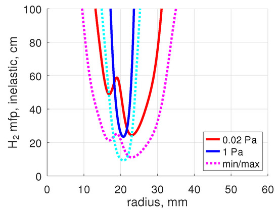
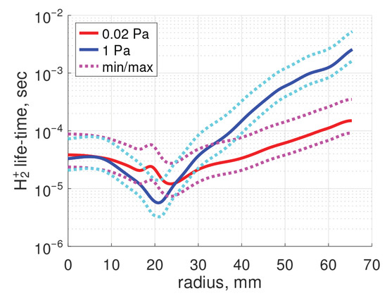
One can see in Table 2 that is always significantly larger than the plasma diameter. Thus, in the plasma in question, no substantial heating of due to collisions with ions is expected. On the contrary, the smallest is comparable to the characteristic plasma size. However, a closer look (Figure 9) shows that smaller than 40–50 cm are only found in an approximately 2 cm thick layer around the location of the maximum . Thus, according to this estimate, depletion of density due to dissociation and ionization is unlikely to be important here as well. Nevertheless, as discussed next, this conclusion could be compromised by neutral–neutral collisions.
Figure 9.
Mean free path of inelastic collisions, , Equation (14). The solid curves are for = 300 K, = 0.1.
The MFP of elastic collisions is estimated using the hard sphere formula:
where is the Lennard-Jones collision diameter, m [52]. As one can see, Table 2, can become smaller than the vacuum vessel diameter (40 cm). At the same time, always stays much larger than the diameter of the tube, which connects the pressure gauge with the vacuum vessel (4 cm). Hence, the assumption of free molecular flow in Section 3.2 is justified in this case.
Elastic collisions between molecules as such cannot lead to significant re-distribution of their density, as long as there are no strong temperature or pressure gradients in the gas. Their major effect could be the increase of the molecules’ residence time in the plasma, thus, effectively increasing depletion of their density there.
The cross-sections of elastic collisions tend to decrease with the increased kinetic energy of the colliding neutral particles [50,53]. Therefore, the estimated MFP of collisions of ballistic H-atoms with molecules are larger than . A calculation for atoms with kinetic energy 3 eV and cross-sections from [50] is shown in Table 2. As one can see, in the 0.02 Pa case, this length is much larger than the vacuum vessel diameter and the collision-free assumption for those atoms is justified.
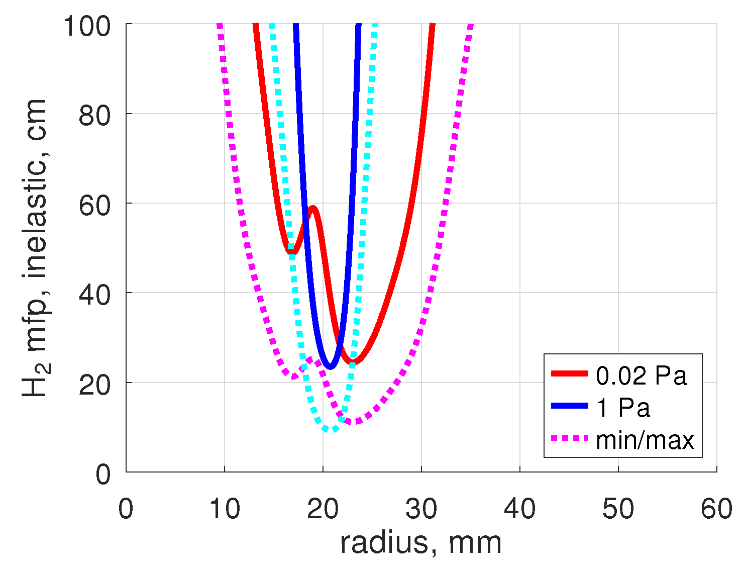
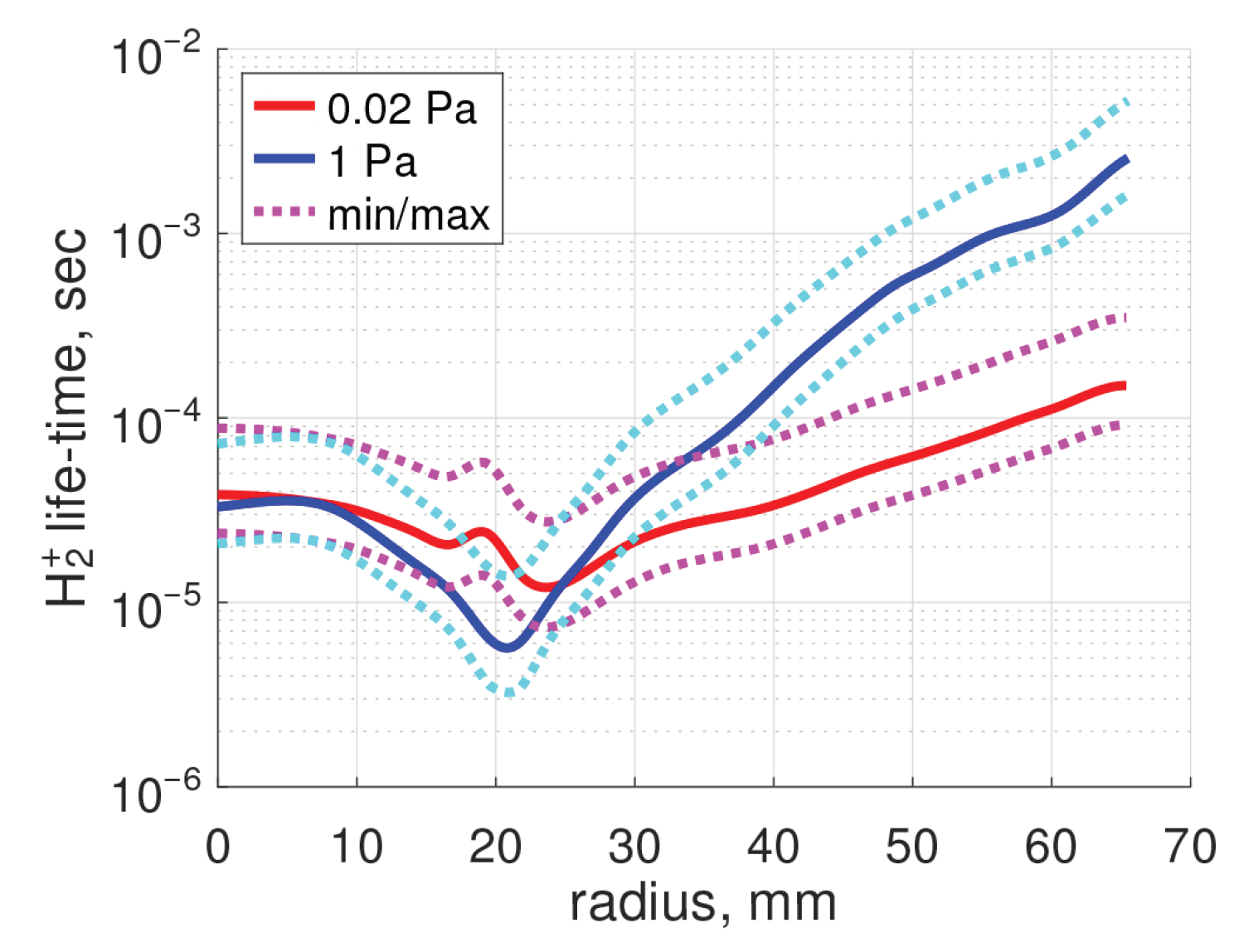
To verify the local 0D approximation used in Section 3.3, the characteristic life-time of ions is calculated:
here , are the rate coefficients of the destruction processes (Table 1). The result is shown in Figure 10. For the local 0D approximation to be applicable, must be smaller than transport times. The order of magnitude of the latter can be estimated as follows:
where is the characteristic time of transport across the magnetic field, ∼1 cm is the radial gradient length of ion density, ∼1 m2/s is the cross-field diffusion coefficient; is the characteristic time of parallel transport, L∼1 m is the characteristic parallel length, and ∼104 m/s is the ion sound speed. The choice of the order of magnitude of for this estimate is based on [29], where cross-field transport in PSI-1 and PSI-2 experiments is discussed. The classical ambipolar diffusivity is of the order of 0.1 m2/s, but, as it is common in magnetized plasmas, the transport is likely to be anomalous. In [29], the best match of the 2D transport simulations with experimental plasma profiles was found with anomalous = 0.5 m2/s.
Figure 10.
Characteristic life-time of ions , Equation (16). The solid curves are for = 300 K, = 0.1.
One can see that , estimated in this very rough way have same order of magnitude as 10−5–10−4 s (Figure 10). That is, although the plasma chemical processes are fast, it cannot be excluded that ion transport can have a non-negligible effect on the local density.
All the population factors and rate coefficients used in the present work are calculated on assumption of optically thin gas. It turns out, however, that the density of H-atoms in this experiment (see the next section) is high enough for the resonance absorption of atomic Lyman lines to start to become significant. Estimated MFPs of Lyman photons can be found in Table 3. They are calculated for the center of Doppler broadened lines according to [54]. The numerical formulas are taken from [55] (Equation (4.12) and Table 4.2 there). The calculations are made assuming the temperature = 0.3 eV for re-emitted (thermal) atoms, and effective temperature 2 eV for ballistic atoms.
Table 3.
Estimated photon mean free paths, center of Doppler broadened line.
The result, expectedly, strongly depends on the assumed surface recombination probability . In the 0.02 Pa case, the gas is guaranteed to be optically thin for . For ∼, the MFPs of become comparable to the plasma size, and for , the opacity could become significant for as well. At the same time, stays transparent. With increased temperature , the MFPs are increased roughly proportional to . The absorption cross-sections of Balmer lines are larger than those of Lyman lines (see, e.g., [55], Table 4.2), but the population of is found to be always <10−3 of the ground state. As a result, in both the 0.02 Pa and 1 Pa cases, MFPs of Balmer photons are always >10 m. That is, no absorption of Balmer lines is expected.
The MFPs obtained for do not automatically imply a strong effect on the intensity of Balmer radiation emitted from the plasma core. First, they are only valid for the line center, whereas the absorption cross-section rapidly reduces as the difference between the photon energy and the resonance energy is increased. Second, as long as non-negligible opacity only takes place for , only the state is directly affected. The radiation from Balmer lines is influenced only indirectly by the electron impact excitations from that state, whose effect at the low electron densities of this experiment is relatively weak. However, it is worth remembering that at the plasma periphery where the electron density gets very low and, subsequently, excitation due to electron impact diminishes, radiation trapping can even become the dominant source of excited atoms.
To conclude, estimates of characteristic lengths and times above back the assumption that in the 0.02 Pa case, collisions of neutral particles with plasma can be neglected and collision-free approximation for ballistic atoms is valid, at least in the first approximation. However, they cannot fully back the validity of the assumption that ion transport can be neglected. In case a substantial amount of H-atoms can be re-emitted from the wall, , opacity of lines can start to become important as well. Thorough theoretical investigation of those effects would require detailed transport and kinetic calculations and is outside of the scope of the present work.
4.3. Model Predictions
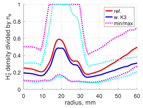
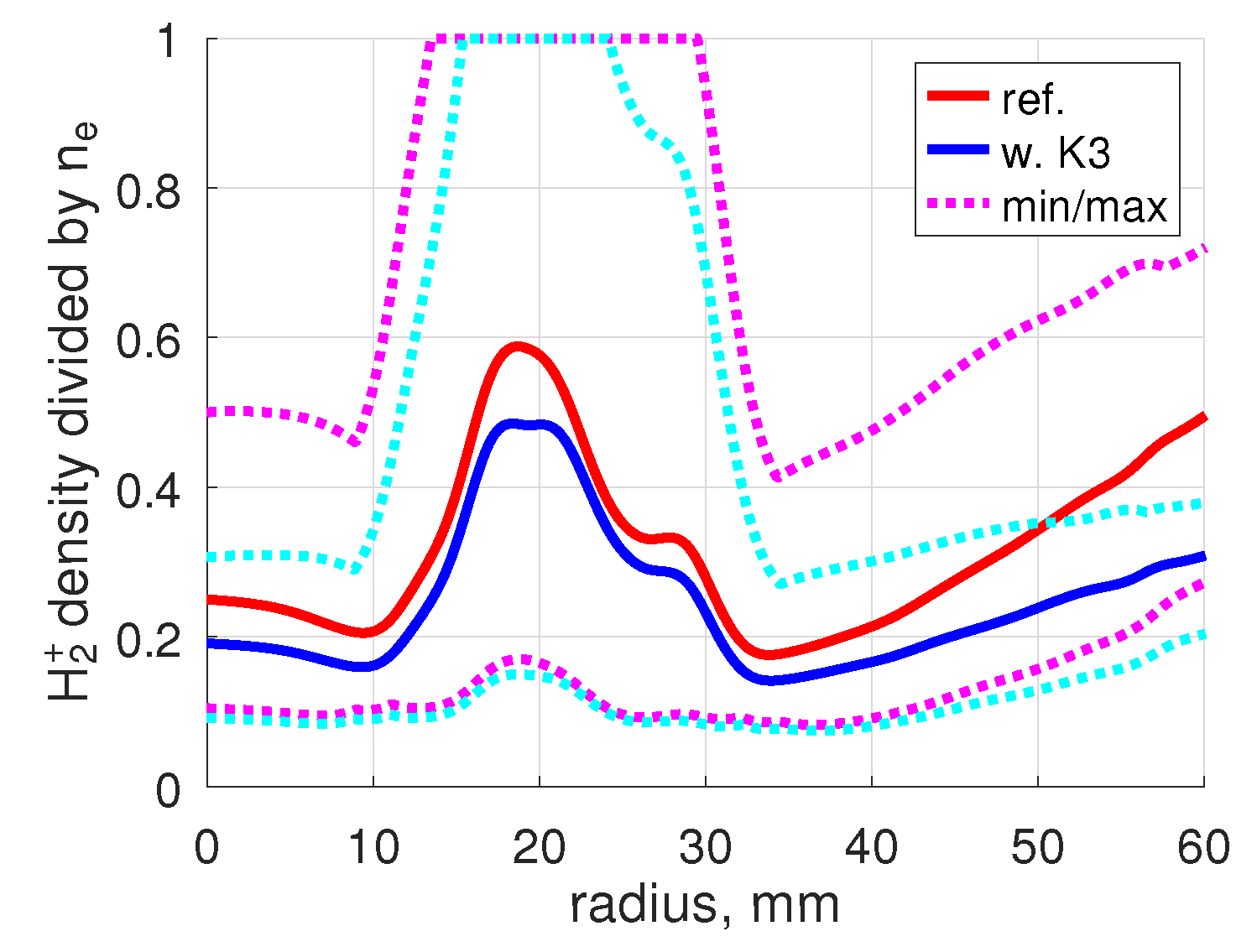
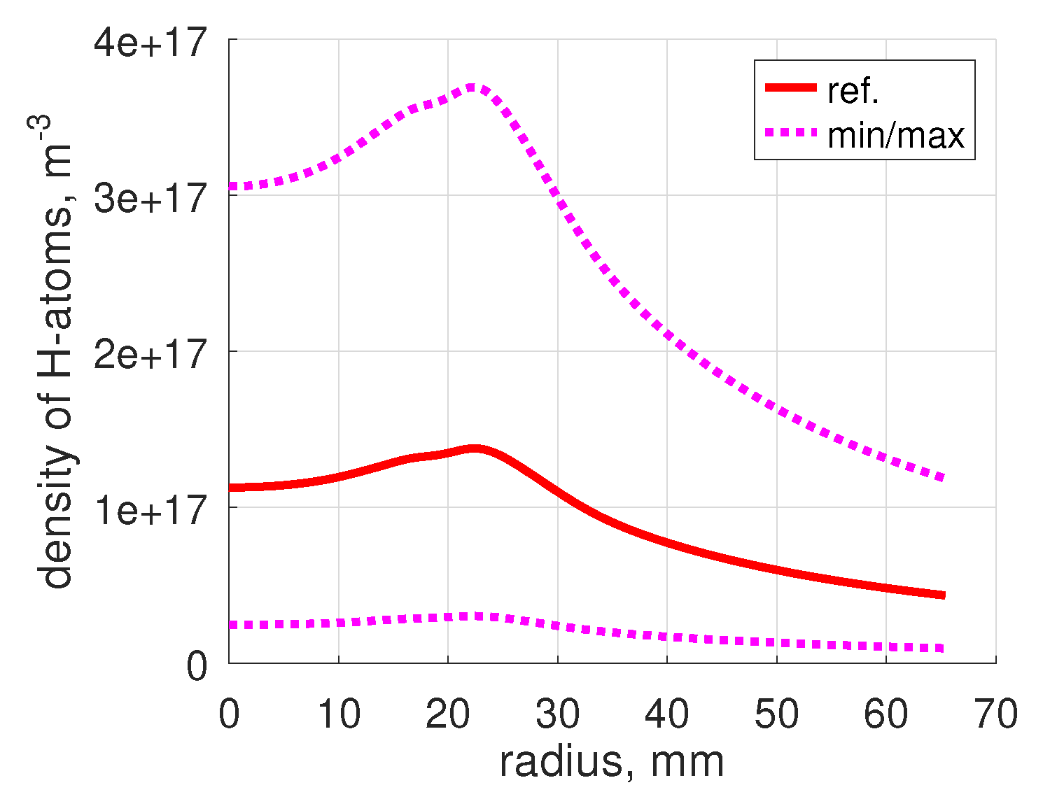
An example of the concentration calculated by the model is shown in Figure 11. The full set for all combinations of parameters , can be found in the Supplementary Materials. There is some variation with and , but it is not stronger than that due to uncertainty of , , . The dependence on and is mainly due to the dependence of on (Equation (5)). There is only weak non-linearity due to modification of density and correction (7). The scattering with varying , is very large.
Figure 11.
Example of the calculated concentration of ions, 0.02 Pa, = 0.1, = 300 K. ‘w. K3’ is a test with the extra destruction process (Table 1) added.
The potential impact of the process (see Table 1) on the calculated was estimated. The rate coefficient [6,36] is a function of the temperature of ions and beam energy of , and is decreased when those two parameters are increased. To obtain an upper estimate, both parameters were set to 0.1 eV, which is the minimal value for which the fit [6,36] is valid. As one can see in Figure 11, in this case, the expected impact on the concentration maximum is very moderate, although the impact may get larger in the plasma center and at the edges. The process competes as a loss term of ions with and . The rate coefficient is roughly 102 times smaller than : therefore, becomes significant and eventually outperforms , only when 100. In the experiment considered, 10…100; therefore, the effect of is still moderate. The obtained modification of the concentration due to process has only a very small effect on the calculated absolute radiation intensities, and a negligible effect on the line intensity ratios; see the Supplementary Materials.
In general, one can say that with the assumed variation of plasma parameters, can vary from ≈10% to 100%. That is, at certain conditions, may be the dominant ion species. This result agrees with previous reconstruction of the density in this same experiment by applying Balmer lines analysis [56]. No direct measurements of the plasma composition in PSI-2 deep in the plasma are available, only one mass-spectrometer measurement at the plasma periphery has been reported by Sorokin et al. [57]. In a D discharge with parameters close to that of the 0.02 Pa case considered here, the concentration at the distance from the plasma axis r = 4 cm found in [57] is around 5%. This value is much lower than at the same location in Figure 11: 20% with reference plasma parameters, down to 10% at the minimum. The difference in the plasma parameters , between H and D discharges in question was found to be moderate, within 10–20%. This difference alone cannot fully explain the large discrepancy with [57].
Especially at the plasma periphery, the effect of transport on the ion concentration could be potentially significant; see Section 4.2 and Figure 10. If, nevertheless, the local 0D approximation holds there than there are two most likely reasons for the discrepancy with the mass-spectrometer measurements. Both are related to process (see Table 1). According to the model, near the position of the , maximum, 1 cm < r < 3 cm (Figure 2), is mainly produced by ionization . At the plasma center, r < 1 cm, and periphery, r > 3 cm, where gets low the is inefficient and ion conversion is the dominant production process. The rate coefficient applied here is calculated on certain assumptions which can be inadequate for the low density plasma in question; see Section 3.1 above. Most importantly the quasi-static approximation for vibrationally excited states of . Besides that, as it was also already discussed in Section 3.1, the rate coefficients , (Table 1) are calculated assuming a certain vibrational distribution of , and can be substantially modified if ionization is not the major source of . Therefore, the density predicted by the present model at the locations where dominates is particularly unreliable and could be overestimated. This is the first possible reason for the discrepancy above. The second reason is the difference between D and H. Opposite to , the effective rate coefficient for D can be significantly smaller than for H [25]. This may lead to a smaller concentration of than that of , even when , are very close.
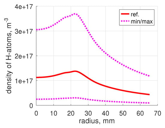
Another quantity of interest calculated by the model, which was not directly measured, is the density of atoms. Figure 12 shows the density of ballistic atoms calculated by applying Equation (A3) of Appendix B. When is around 0.1, the total density is determined almost entirely by thermal (re-emitted) atoms; its value is then around 1018 m−3 or higher. For also, the fraction of atoms in the total flux measured by pressure gauge, the term in Equation (3), can be significant. This fraction is only 1–5% for , but is increased up to 7–30% for = 0.1, and up to 10–50% for = 0.05.
Figure 12.
Example of the density of ballistic H-atoms, 0.02 Pa, = 300 K.
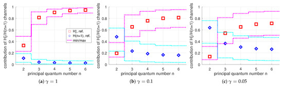
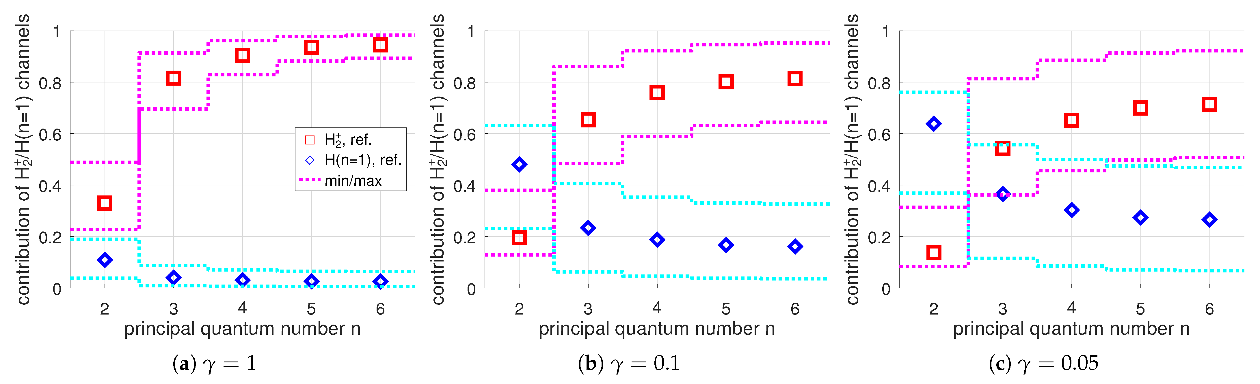
As it was already mentioned in Section 3.1 above, a simple consideration based on the observed intensity ratio already leads to the conclusion that the channel likely dominates the Balmer radiation in this experiment. This consideration is confirmed by the model calculations. The relative contribution of different channels into the population of excited states is presented in Figure 13. In this figure, the ratios of the integrals over lines of sight of the individual terms of Equation (1) and the sum over all terms are shown. The ratios shown are calculated for the central chord, height = 0, but they stay approximately the same within 2 cm around the center; see the Supplementary Materials. Only calculations with = 300 K are shown because the result is not sensitive to . One can clearly see that although the importance of the excitation from ground state, the channel, is expectedly increased with decreased , for = 0.1–1, the contribution of the channel into the population of states is dominant. The contribution is always relatively small, ≈20% for n = 3, and is further reduced when n is increased.
Figure 13.
Calculated contributions of the and channels into population of excited atoms , 0.02 Pa case, = 300 K, integrals over central chord.
As extra information, the level whose radiation was not accessible to the present measurements is added to the plots in Figure 13. For that level, the breakdown over individual excitation channels differs strongly from . The contribution of the channel is much smaller, although still not insignificant. The contribution of is comparable to or even stronger. It is worth mentioning that the state can be also effectively populated by the channel, the process [6], which was not taken into account here. Also in case , the impact of the absorption of radiation on the population of that state could be non-negligible; see Section 4.2 above. Although, latter effect is expected to be important for line of sights going through the plasma periphery rather than over the central chord.
5. Results for 1 Pa Case
Besides the higher neutral density, the main difference in the 1 Pa experiment and the 0.02 Pa case is significantly lower temperature ; see Figure 2a. Similarly to the previous section, the assumptions underlying the model of Section 3 are verified by applying the model itself and evaluating the results. With elevated pressure, the validity of the simplified approach without detailed transport modeling used here turns out to be far less justified than in the 0.02 Pa case. The following issues were identified:
- 1.
- MFP of collisions of ballistic atoms with molecules is comparable to the vacuum vessel diameter (Table 2). The no-collision assumption for those atoms is thus no longer strictly valid.
- 2.
- The estimated MFP of elastic collisions (Table 2) is so short that even the assumption of collision-free flow in the pressure gauge inlet (Section 3.2) becomes questionable.
- 3.
- Other MFPs are not substantially smaller than in the 0.02 Pa case (Table 2 and Figure 9), but collisions can lead to larger effective dwell time of molecules in the plasma. Hence, the depletion of molecule density can be more significant than that expected from formal comparison of MFPs with plasma size.
- 4.
- The characteristic life-time close to the plasma center is similar to that in the 0.02 Pa case (Figure 10), but is up to an order of magnitude larger at radius > 3 cm.
- 5.
- MPFs of (Table 3) can become comparable to the plasma diameter even in the absence of re-emission of atoms from the wall, . If , then is almost guaranteed opaque, and even can be expected to become opaque under those conditions.
- 6.
- Moreover, since no-bulk-collisions approximation does not hold anymore, even for , the calculated atom density can be underestimated. Thus, the MFP of is realistically even smaller than the values suggested by the present estimate.
To summarize, the main issues are potential effects of neutral–neutral collisions and absorption of Lyman lines.
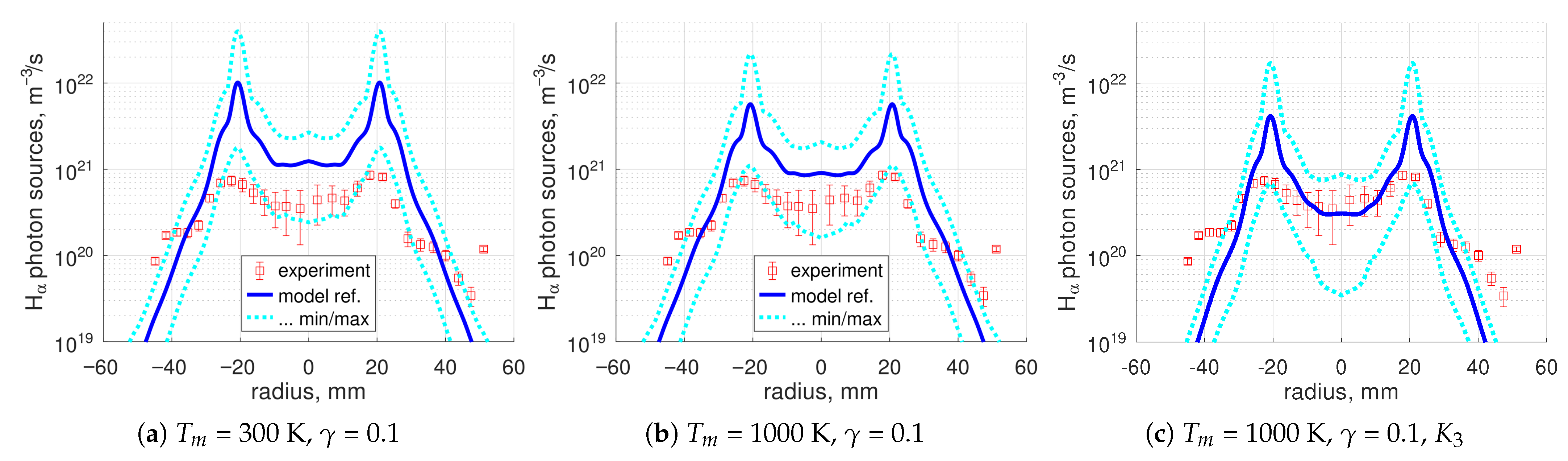
Taking into account the issues listed above, the present modeling approach is apparently not appropriate for the 1 Pa case. Nevertheless, for the record, comparison of this model with the measurements was documented. Examples are shown in Figure 14 and Figure 15; the full set can be found in the Supplementary Materials. The potential effect of process (Table 1) was estimated in the same way as in Section 4.3 as well. The effect is much stronger than in the 0.02 Pa case: the concentration of is reduced by a factor 1.5–3, with subsequent substantial reduction in the absolute photon sources (Figure 14c).
Figure 14.
The 1 Pa case, absolute photon sources, (c) is a test with process (Table 1) added.
Figure 15.
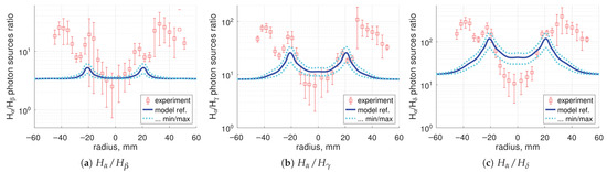
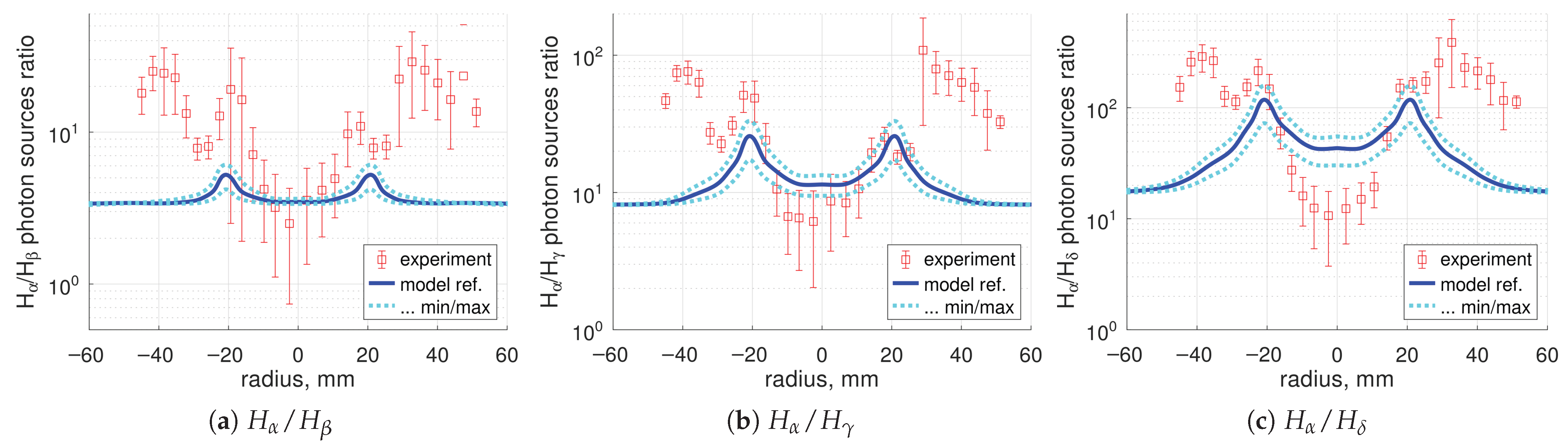
The 1 Pa case, lines emissivities ratios, , = 1000 K.
Expectedly, the calculations cannot reproduce both the absolute radiation and the line intensity ratios. The most prominent disagreement is that at the plasma periphery (radius cm) where the model very strongly, by an order of magnitude, underestimates the intensity of with respect to other lines (Figure 15). The reasons for that may be related to the non-local effects of vibrational kinetics and to radiation trapping. The rate coefficients used in the baseline plasma chemical mechanism, with the exception of process , do not take into account vibrational states of . Vibrationaly excited molecules could enhance the radiation due to the channel in the low regions, shifting the line ratios towards (see Figure 5). Absorption of and, especially, photons at the plasma periphery can also lead to an increased population there.
6. Conclusions
Spatially resolved absolute intensities of the atomic lines , , , were measured and analyzed in pure hydrogen plasma in the linear plasma device PSI-2. Two regimes were investigated, with low (‘0.02 Pa’) and high (‘1 Pa’) gas pressure (see the comment on the pressure gauge reading in Section 2.2). A very clear difference in terms of the line radiation intensity ratios is observed between the two experimental regimes. Population factors calculated by collision-radiative models are applied to analyze the measured radiation. In the 0.02 Pa regime, the intensity ratio readily suggests that the dominant source of Balmer radiation is decomposition of . This observation is confirmed by more detailed calculations.
The measurements were compared with model calculations in local 0D approximation for ions and constant density approximation for molecules. Input for the modeling are the plasma parameters , determined by Langmuir probe and the density deduced from the pressure gauge measurements. Excitation from the ground state of , and excitation channels are taken into account. The plasma chemical mechanism ‘ITER 2005’ [22,23] was applied to calculate the density. Both the mechanism ‘ITER 2005’ and the population factors used are based on the Sawada–Fujimoto collision-radiative model for atomic and molecular hydrogen [8,32].
For the 0.02 Pa case, both the absolute radiation intensity and the line intensity ratios can be reproduced by the calculations, with exception of the ratio. The model suggests that majority of the observed Balmer radiation is due to channel. The result can be seen as—partial—validation of the mechanism ‘ITER 2005’ and Sawada–Fujimoto population factors for the parameter range in question: = 2–10 eV, ∼ m−3.
For the 1 Pa case with lower temperature = 1–5 eV, the applied simplified approach without detailed transport modeling was found to not be appropriate. In particular, in this case, mutual collisions between neutral particles and opacity of Lyman radiation of hydrogen atoms apparently cannot be neglected. Expectedly, for this experiment, the calculations with the present model have not reproduced the measurements. There are also signs that the baseline plasma chemical mechanism ‘ITER 2005’ is not sufficient for the conditions with elevated pressure because it misses the kinetics of ions and detailed vibrational kinetics of and .
The imaging spectrometer measurements in the discharges with elevated gas pressure can serve in the future as a good benchmark for more detailed mechanisms of hydrogen plasma chemistry and transport, e.g., those developed for negative ion sources [3,58]. In addition to atomic lines, the measurements of molecular bands will be mandatory for evaluation of the mechanisms with detailed vibrational kinetics. Intensities of the molecular Fulcher- bands can be obtained with the same optical imaging spectrometer as the Balmer lines. The largest uncertainty is expected to be the H-atoms density, which was found to be difficult to calculate because of its critical dependence on the surface recombination probability. Direct experimental determination of the atomic density could be a better alternative to calculations.
Despite relatively good agreement of the calculated radiation intensities in the 0.02 Pa case, the absolute value of the concentration obtained here should be taken with caution. Whereas the line intensity ratios can be matched partly with high precision, a “good agreement” of the absolute radiation means, in practice, agreement within a factor ≈2. The magnitude of the variation of the calculated with respect to uncertain parameters is found to be even stronger. Thus, the model of the present work (even if adjusted to experimental radiation intensities; see [56]), cannot be considered as a quantitative diagnostic for determination of . The result that the channel is the dominant source of Balmer radiation does not automatically imply high . To determine the plasma composition with a reliable level of accuracy, direct measurements should be preferred when available, such as mass-spectrometry [57].
Supplementary Materials
The following supporting information can be downloaded at: https://www.mdpi.com/article/10.3390/plasma9020011/s1, Full set of calculations for the 0.02 Pa case, PSI2_model3_results_02Pa.pdf, and the 1 Pa case, PSI2_model3_results_1Pa.pdf. Estimate of the effect of process : PSI2_model3_effect_of_K3.pdf.
Author Contributions
Conceptualization, V.K. and S.B.; methodology, V.K. and G.S.; software, V.K.; validation, M.S. and O.M.; formal analysis, V.K.; investigation, M.S., O.M., M.R. and M.G.; data curation, M.S. and M.R.; writing—original draft preparation, V.K.; writing—review and editing, O.M., M.G. and A.K.; visualization, V.K.; supervision, O.M., G.S. and A.K.; project administration, A.K. and B.U.; funding acquisition, B.U. and S.B. All authors have read and agreed to the published version of the manuscript.
Funding
This work has been carried out within the framework of the EUROfusion Consortium, funded by the European Union via the Euratom Research and Training Programme (Grant Agreement No 101052200 - EUROfusion). Views and opinions expressed are however those of the author(s) only and do not necessarily reflect those of the European Union or the European Commission. Neither the European Union nor the European Commission can be held responsible for them.
Data Availability Statement
The original contributions presented in this study are included in the article/Supplementary Materials. Further inquiries can be directed to the corresponding author.
Conflicts of Interest
The authors declare no conflicts of interest.
Abbreviations
The following abbreviations are used in this manuscript:
| LPD | Linear Plasma Device |
| MFP | Mean Free Path |
Appendix A. Integral over Spectral Line S with Background Separation and Error Estimate ΔS
First, pixels that correspond to the ‘beginning’ b and the ‘end’ e of the line are determined. Then, the sum is calculated, where is the number of counts in the pixel i. The integral over the spectral line is then found by subtracting the estimated ‘background radiation’ beneath the isolated line itself: . The impact of the uncertainty in determining b and e on the calculated S is estimated by moving the ‘beginning’ and ‘end’ pixels further to the left and to the right, approximately over pixels to each side. For each extended set of pixels , the integral is calculated. As the error estimate of S the maximum deviation over all sets, is taken. This error estimate is conservative and may lead to strong overestimation of the real error of S. Nevertheless, it was found more practical to exclude lines of sight for which this procedure detects errors that are too large rather than to try a more sophisticated integration and error estimation algorithm.
Appendix B. Ballistic Calculation of the Density of Particles Emitted by Isotropic Cylindrically Symmetric Source
The following problem is considered. To find the number density of particles emitted by a cylindrically symmetric volumetric source S, uniform and infinite in axial direction. The particles experience no collisions. The source is isotropic; all particles have same absolute velocity u. Single-speed transport of neutral particles is a problem well known in radiation transport theory [59] and neutronics [60]. The solution can be found as a superposition of the point sources:
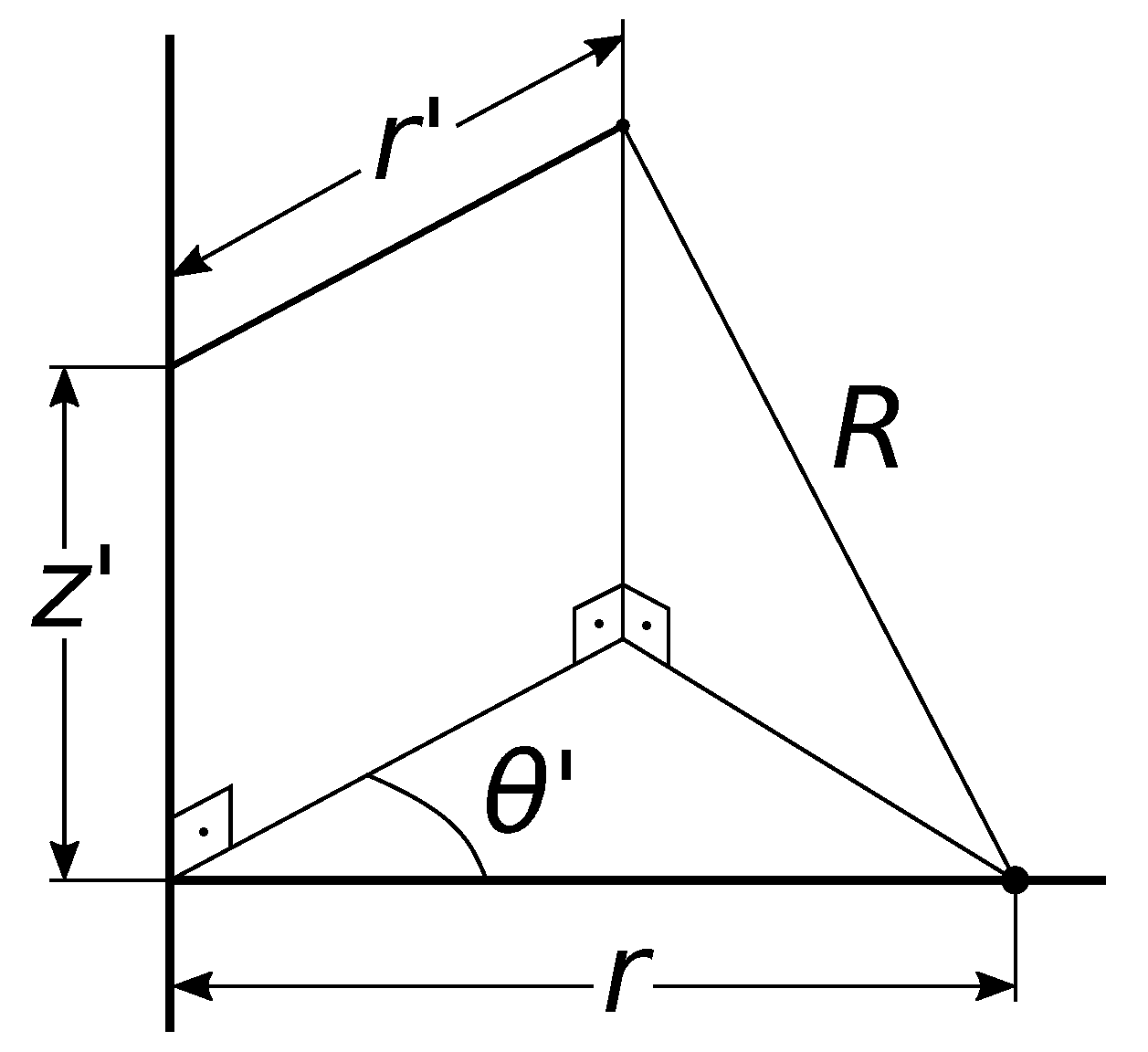
where is the source strength, and R is the distance from the source to the point where the density is calculated. For the distributed source S, the source strength is replaced by , and integration over volume V is performed in cylindrical coordinates (Figure A1). Because of the symmetry of the problem, the solution will depend only on the radial coordinate r. As readily seen from Figure A1:
Then
Since :
Figure A1.
Towards definition of the integral (A1) in Appendix B.
The integral over is expressed via elliptic integrals by substituting :
is the elliptic integral of the first kind; see [61] (Chapter 17). Transformation of into canonical form can be found in [61] (Section 17.4.17):
where
is the complete elliptic integral of the first kind; see [61] (Chapter 17.4). Substituting the results of the integration over into (A2) yields the final formula:
The integrand of Equation (A3) has singularity at , where . From the physics meaning the integral must stay finite, but there was found no strict mathematical proof of that. When (A3) is evaluated numerically, a small interval around is excluded.
Two useful special cases are available. The first is for ; it can be obtained from (A3) taking into account that , or directly from (A2):
The second is the case of the source S localized within some radius such that . Then for , and thus :
The expression in parentheses is the strengths per unit length of a cylindrical source and the formula for is exactly the same as that derived in one-speed neutron transport theory for a line isotropic source, Equation (9.44) in [60], with absorption set to zero.
References
- Fridman, A.A. Plasma Chemistry; Cambridge University Press: Cambridge, UK, 2008. [Google Scholar]
- Profijt, H.B.; Potts, S.E.; van de Sanden, M.C.M.; Kessels, W.M.M. Plasma-assisted atomic layer deposition: Basics, opportunities, and challenges. J. Vac. Sci. Technol. 2011, A29, 050801. [Google Scholar] [CrossRef] [Scilit]
- Bacal, M. Physics and Applications of Hydrogen Negative Ion Sources; Springer: Cham, Switzerland, 2023. [Google Scholar]
- Krasheninnikov, S.I.; Smolyakov, A.I.; Kukushkin, A.S. On the Edge of Magnetic Fusion Devices; Springer: Cham, Switzerland, 2020. [Google Scholar]
- Ohno, N. Plasma detachment in linear devices. Plasma Phys. Control. Fusion 2017, 59, 034007. [Google Scholar] [CrossRef] [Scilit]
- Janev, R.K.; Langer, W.D.; Evans, K.; Post, D.E. Elementary Processes in Hydrogen-Helium Plasmas; Springer: Berlin, Germany, 1987. [Google Scholar]
- Fujimoto, T.; Sawada, K.; Takahata, K. Ratio of Balmer line intensities resulting from dissociative excitation of molecular hydrogen in an ionizing plasma. J. Appl. Phys. 1989, 66, 2315–2319. [Google Scholar] [CrossRef] [Scilit]
- Sawada, K.; Fujimoto, T. Effective ionization and dissociation rate coefficients of molecular hydrogen in plasma. J. Appl. Phys. 1995, 78, 2913–2924. [Google Scholar] [CrossRef] [Scilit]
- Schmitz, L.; Merriman, B.; Blush, L.; Lehmer, R.; Conn, R.W.; Doerner, R.; Grossman, A.; Najmabadi, F. Plasma and neutral dynamics in a simulated tokamak gas target divertor. Phys. Plasmas 1995, 2, 3081–3094. [Google Scholar] [CrossRef] [Scilit]
- Hollmann, E.M.; Pigarov, A.Y.; Seraydarian, R.; Whyte, D.G.; Krasheninnikov, S.I. Particle balance measurements during detachment in a gas-target divertor simulator. Phys. Plasmas 2002, 9, 1226–1232. [Google Scholar] [CrossRef] [Scilit]
- Ohno, N.; Ezumi, N.; Takamura, S.; Krasheninnikov, S.I.; Pigarov, A.Y. Experimental evidence of molecular activated recombination in detached recombining plasmas. Phys. Rev. Lett. 1998, 81, 818–821. [Google Scholar] [CrossRef] [Scilit]
- Ezumi, N.; Nishijima, D.; Kojima, H.; Ohno, N.; Takamura, S.; Krasheninnikov, S.I.; Pigarov, A.Y. Contribution of molecular activated recombination to hydrogen plasma detachment in the divertor plasma simulator NAGDIS-II. J. Nucl. Mater. 1999, 266–269, 337–342. [Google Scholar] [CrossRef] [Scilit]
- Sakamoto, M.; Terakado, A.; Nojiri, K.; Ezumi, N.; Nakashima, Y.; Sawada, K.; Ichimura, K.; Fukumoto, M.; Oki, K.; Shimizu, K.; et al. Molecular activated recombination in divertor simulation plasma on GAMMA 10/PDX. Nucl. Mater. Energy 2017, 12, 1004–1009. [Google Scholar] [CrossRef] [Scilit]
- Akkermans, G.R.A.; Classen, I.G.J.; Perillo, R.; van der Meiden, H.J.; Federici, F.; Brezinsek, S. The role of hydrogen molecular effects on detachment in Magnum-PSI. Phys. Plasmas 2020, 27, 102509. [Google Scholar] [CrossRef] [Scilit]
- Kreter, A.; Brandt, C.; Huber, A.; Kraus, S.; Möller, S.; Reinhart, M.; Schweer, B.; Sergienko, G.; Unterbertg, B. Linear Plasma Device PSI-2 for Plasma-Material Interaction Studies. Fusion Sci. Technol. 2015, 68, 8–14. [Google Scholar] [CrossRef] [Scilit]
- Meyer, H.; Klose, S.; Pasch, E.; Fussmann, G. Plasma rotation in a plasma generator. Phys. Rev. E 2000, 61, 4347–4356. [Google Scholar] [CrossRef] [Scilit]
- Wenzel, U.; Schröder, D.; Fussmann, G. Appearance of a Hα Minimum at the Onset of Net Recombination in Hydrogen Plasmas. Contrib. Plasma Phys. 2007, 47, 451. [Google Scholar] [CrossRef] [Scilit]
- Waldmann, O.; Meyer, H.; Fussmann, G. Anomalous Diffusion in a Linear Plasma Generator. Contrib. Plasma Phys. 2007, 47, 691–702. [Google Scholar] [CrossRef] [Scilit]
- Pospieszczyk, A.; Reinhart, M.; Unterberg, B.; Brezinsek, S.; Kreter, A.; Samm, U.; Sergienko, G.; Schweer, B.; Salmagne, C.; Reiter, D.; et al. Spectroscopic characterisation of the PSI-2 plasma in the ionising and recombining state. J. Nucl. Mater. 2013, 438, S1249–S1252. [Google Scholar] [CrossRef] [Scilit]
- Reinhart, M.; Pospieszczyk, A.; Unterberg, B.; Brezinsek, S.; Kreter, A.; Samm, U.; Sergienko, G.; Schweer, B.; Reiter, D.; Wünderlich, D.; et al. Using the Radiation of Hydrogen Atoms and Molecules to Determine Electron Density and Temperature in the Linear Plasma Device PSI-2. Fusion Sci. Technol. 2013, 631T, 201–204. [Google Scholar] [CrossRef] [Scilit]
- Marchuk, O.; Brandt, C.; Pospieszczyk, A.; Reinhart, M.; Brezinsek, S.; Unterberg, B.; Dickheuer, S. Emission of fast hydrogen atoms at a plasma–solid interface in a low density plasma containing noble gases. J. Phys. B At. Mol. Opt. Phys. 2018, 51, 025702. [Google Scholar] [CrossRef] [Scilit]
- Reiter, D.; May, C.; Baelmans, M.; Börner, P. Non-linear effects on neutral gas transport in divertors. J. Nucl. Mater. 1997, 241–243, 342–348. [Google Scholar] [CrossRef] [Scilit]
- Kukushkin, A.S.; Pacher, H.D.; Kotov, V.; Reiter, D.; Coster, D.P.; Pacher, G.W. Effect of neutral transport on ITER divertor performance. Nucl. Fusion 2005, 45, 608–616. [Google Scholar] [CrossRef] [Scilit]
- Krasheninnikov, S.I.; Kukushkin, A.S.; Pshenov, A.A. Divertor plasma detachment. Phys. Plasmas 2016, 23, 055602. [Google Scholar] [CrossRef] [Scilit]
- Kukushkin, A.S.; Krasheninnikov, S.I.; Pshenov, A.A.; Reiter, D. Role of molecular effects in divertor plasma recombination. Nucl. Mater. Energy 2017, 12, 984–988. [Google Scholar] [CrossRef] [Scilit]
- Pfeiffer Vacuum. Betriebsanleitung. PKR 251, Pirani/Kaltkathoden Transmitter. Available online: https://www.idealvac.com/files/ManualsII/Pfeiffer_PKR_251_Pirani_ColdCathode.pdf?srsltid=AfmBOoozSfYYGTSNzdFk8RpYzXcHC542Ot0Eq5pWlGHuXPkWCRjELXhH (accessed on 30 October 2024).
- Demidov, V.I.; Ratynskaia, S.V.; Rypdal, K. Electric probes for plasmas: The link between theory and instrument. Rev. Sci. Instrum. 2002, 73, 3409–3439. [Google Scholar] [CrossRef] [Scilit]
- Matthews, G.F. Tokamak plasma diagnosis by electrical probes. Plasma Phys. Control. Fusion 1994, 36, 1595. [Google Scholar] [CrossRef] [Scilit]
- Kastelewicz, H.; Fussmann, G. Plasma Modelling for the PSI Linear Plasma Device. Contrib. Plasma Phys. 2004, 44, 352–360. [Google Scholar] [CrossRef] [Scilit]
- Wünderlich, D.; Dietrich, S.; Fantz, U. Application of a collisional radiative model to atomic hydrogen for diagnostic purposes. J. Quant. Spectrosc. Radiat. Transf. 2009, 110, 62–71. [Google Scholar] [CrossRef] [Scilit]
- Fantz, U.; Wünderlich, D. Atomic and Molecular Collisional Radiative Modeling for Spectroscopy of Low Temperature and Magnetic Fusion Plasmas. AIP Conf. Proc. 2011, 1344, 204–216. [Google Scholar] [CrossRef] [Scilit]
- Sawada, K.; Eriguchi, K.; Fujimoto, T. Hydrogen-atom spectroscopy of the ionizing plasma containing molecular hydrogen: Line intensities and ionization rate. J. Appl. Phys. 1993, 73, 8122–8125. [Google Scholar] [CrossRef] [Scilit]
- Greenland, P.T.; Reiter, D. The Role of Molecular Hydrogen in Plasma Recombination. Report Jül-3258. 1996. Available online: http://hdl.handle.net/2128/21698 (accessed on 1 December 2016).
- Reiter, D. The Data File AMJUEL: Additional Atomic and Molecular Data for EIRENE. Available online: https://www.eirene.de/Documentation/amjuel.pdf (accessed on 1 December 2016).
- Janev, R.K.; Reiter, D.; Samm, U. Collision Processes in Low-Temperature Hydrogen Plasmas. Report Jül-4105. 2003. Available online: http://hdl.handle.net/2128/249 (accessed on 1 December 2016).
- Reiter, D. The Data File HYDHEL: Atomic and Molecular Data for EIRENE Based upon: Janev, Langer, Evans, Post, “Elementary Processes in Hydrogen-Helium Plasmas”, Springer 1987. Available online: https://www.eirene.de/Documentation/hydhel.pdf (accessed on 1 December 2016).
- Wünderlich, D.; Giacomin, M.; Ritz, R.; Fantz, U. Yacora on the Web: Online collisional radiative models for plasmas containing H, H2 or He. J. Quant. Spectrosc. Radiat. Transf. 2020, 240, 106695. [Google Scholar] [CrossRef] [Scilit]
- Available online: https://www.yacora.de/ (accessed on 24 February 2025).
- Hofman, M.S.; Wang, D.Z.; Yang, Y.; Koel, B.E. Interactions of incident H atoms with metal surfaces. Surf. Sci. Rep. 2018, 73, 153–189. [Google Scholar] [CrossRef] [Scilit]
- Capitelli, M.; Ferreira, C.M.; Gordiets, B.F.; Osipov, A.I. Plasma Kinetics in Atmospheric Gases; Springer: Berlin, Germany, 2000. [Google Scholar]
- Stangeby, P.C. Interpretation of Langmuir, heat-flux, deposition, trapping and gridded energy analyser probe data for impure plasmas. J. Phys. D Appl. Phys. 1987, 20, 1472–1478. [Google Scholar] [CrossRef] [Scilit]
- Tskhakaya, D.; Kuhn, S.; Tomita, Y. Formulation of Boundary Conditions for the Unmagnetized Multi-Ion-Component Plasma Sheath. Contrib. Plasma Phys. 2006, 46, 649–654. [Google Scholar] [CrossRef] [Scilit]
- Cottingham, W.B.; Grosh, R.J. Surface Recombination and Heat Transfer in a Dissociated Diatomic Gas—Part 1. J. Heat Transf. 1963, 85, 101–106. [Google Scholar] [CrossRef] [Scilit]
- Melin, A.; Madix, R.J. Energy accommodation during hydrogen atom recombination on metal surfaces. Trans. Faraday Soc. 1971, 67, 2711–2719. [Google Scholar] [CrossRef] [Scilit]
- Mozetič, M.; Drobnič, M.; Zalar, A. Recombination of neutral hydrogen atoms on AISI 304 stainless steel surface. Appl. Surf. Sci. 1999, 144–145, 399–403. [Google Scholar] [CrossRef] [Scilit]
- Gubarev, V.; Lopaev, D.; Zotovich, A.; Medvedev, V.; Krainov, P.; Astakhov, D.; Zyryanov, S. Dynamics of H atoms surface recombination in low-temperature plasma. J. Appl. Phys. 2022, 132, 193301. [Google Scholar] [CrossRef] [Scilit]
- Sode, M.; Schwarz-Selinger, T.; Jacob, W.; Kersten, H. Surface loss probability of atomic hydrogen for different electrode cover materials investigated in H2-Ar low-pressure plasmas. J. Appl. Phys. 2014, 116, 013302. [Google Scholar] [CrossRef] [Scilit]
- Stodolna, A.S.; Ramankutty, S.; Blauw, M.; de Jonge, T.; Storm, A.J.; Velthuis, J.F.M. Measurements of atomic hydrogen recombination coefficients and the reduction of Al2O3 using a heat flux sensor. J. Vac. Sci. Technol. 2024, 42A, 053003. [Google Scholar] [CrossRef] [Scilit]
- Eerden, M.J.J.; va de Sanden, M.C.M.; Otorbaev, D.K.; Schram, D.C. Cross section for the mutual neutralization reaction + H−, calculated in a multiple-crossing Landau-Zener approximation. Phys. Rev. A 1995, 51, 3362–3365. [Google Scholar] [CrossRef] [Scilit] [PubMed]
- Phelps, A.V. Cross Sections and Swarm Coefficients for H+, H2+, H3+, H, H2, and H- in H2 for Energies from 0.1 eV to 10 keV. J. Phys. Chem. Ref. Data 1990, 19, 653–675. [Google Scholar] [CrossRef] [Scilit]
- Bachmann, P.; Reiter, D. Kinetic Description of Elastic Processes in Hydrogen-Helium Plasmas. Contrib. Plasma Phys. 1995, 35, 45–100. [Google Scholar] [CrossRef] [Scilit]
- Poling, B.E.; Prausnitz, J.M.; O’Connell, J.P. The Properties of Gases and Liquids, 5th ed.; McGRAW-HILL: New York, NY, USA, 2001. [Google Scholar]
- Krstić, P.S.; Schultz, D.R. Consistent definitions for, and relationships among, cross sections for elastic scattering of hydrogen ions, atoms, and molecules. Phys. Rev. A 1999, 60, 2118–2130. [Google Scholar] [CrossRef] [Scilit]
- Sobelman, I.I.; Vainstein, L.A.; Yukov, E.A. Excitation of Atoms and Broadening of Spectral Lines; Springer: Berlin, Germany, 1998. [Google Scholar]
- Kotov, V.; Reiter, D.; Kukushin, A.S. Numerical Study of the ITER Divertor Plasma with the B2-EIRENE Code Package. Report Jül-4257. 2007. Available online: http://hdl.handle.net/2128/13947 (accessed on 1 December 2016).
- Kotov, V.; Sackers, M.; Reinhart, M.; Marchuk, O.; Sergienko, G.; Kreter, A.; Brezinsek, S. Overview of the optical emission analysis of the hydrogen gas puff experiments in the linear plasma device PSI-2. In Proceedings of the 51st EPS Conference on Plasma Physics, Vilnius, Lithuania, 7–11 July 2025; P4.210, ECA 51A. Available online: https://lac913.epfl.ch/epsppd3/2025/html/PDF/P4_210.pdf (accessed on 1 December 2016).
- Sorokin, I.A.; Vizgalov, I.V.; Kurnaev, V.A.; Brandt, C.; Kreter, A.; Linsmeier, C. In-situ mass-spectrometer of magnetized plasmas. Nucl. Mater. Energy 2017, 12, 1243–1247. [Google Scholar] [CrossRef] [Scilit]
- Yang, W.; Averkin, S.N.; Khrabrov, A.V.; Kaganovich, I.D.; Wang, Y.N.; Aleiferis, S.; Svarnas, P. Benchmarking and validation of global model code for negative hydrogen ion sources. Phys. Plasmas 2018, 25, 113509. [Google Scholar] [CrossRef] [Scilit]
- Carminati, R.; Schotland, J.C. Principles of Scattering and Transport of Light; Cambridge University Press: Cambridge, UK, 2021. [Google Scholar]
- Stacey, W.M. Nuclear Reactor Physics, 3rd ed.; Wiley-VCH: Weinheim, Germany, 2018. [Google Scholar]
- Abramowitz, M.; Stegun, I. Handbook of Mathematical Functions, 9th ed.; Dover Publications: New York, NY, USA, 1972. [Google Scholar]

Disclaimer/Publisher’s Note: The statements, opinions and data contained in all publications are solely those of the individual author(s) and contributor(s) and not of MDPI and/or the editor(s). MDPI and/or the editor(s) disclaim responsibility for any injury to people or property resulting from any ideas, methods, instructions or products referred to in the content. |
© 2026 by the authors. Licensee MDPI, Basel, Switzerland. This article is an open access article distributed under the terms and conditions of the Creative Commons Attribution (CC BY) license.