


Abstract
Railway logistics terminals are crucial nodes in the national logistics system. Prior to the market-oriented reform of railway logistics, the warehousing operations at these stations primarily focused on temporary storage services before and after shipment, making it difficult to provide customers with integrated warehousing and transportation logistics services. With the advancement of railway marketization reforms, railway logistics terminals have gradually begun to offer socialized warehousing services, acquiring the capability to provide integrated warehousing and transportation services. In response to market development needs and the requirements for green development in railway logistics, an optimization design model for obtaining green railway logistics solutions is established, considering factors such as carbon emission costs, integrated warehousing and transportation logistics service costs, fuzzy constraints on logistics network capability, transportation time windows and the customer’s risk tolerance level. The model takes minimizing carbon emission costs and railway logistics service costs as dual-objective functions and uses a standardized weighting method to convert the dual-objective functions into a single-objective function for solving using triangular fuzzy numbers to characterize the ability constraints of network nodes, making the model more realistic. This model aims to minimize these costs and assesses the impact of factors such as changes in delivery time limits, shipment quantity, shipment batches, the superposition of multiple goods batches and customer preferences on the railway logistics solution for different scenarios. Research indicates that reasonably designing delivery time limits and aligning shipment times with railway transportation time windows can effectively reduce carbon emissions and logistics costs, and the risk tolerance level has a significant impact on the reliability of railway logistics solutions.
1. Introduction
Chinese modernization is the modernization of green development, and railway transportation plays a key role in the field of green transportation systems. With the continuous promotion of market-oriented reform in railway logistics, providing customers with integrated and green warehousing, transportation, and comprehensive logistics services is an important development direction for railway logistics enterprises. Networking is the core competitive advantage of railway warehousing resources. By utilizing the nationwide railway warehousing resource network, railway logistics enterprises can provide customers with cross-regional, high-capacity, and convenient freight transportation and warehousing services.
At the end of 2024, the total operating mileage of railways in China was 162,000 km, with more than 3600 operating stations, including about 2960 operating stations with railway freight yards and about 2700 operating stations with railway sidings. Since 2023, China State Railway Group Co., Ltd. has accelerated the construction of a modern railway logistics system and achieved rapid development in railway modern logistics business. The company has established 40 railway logistics centers throughout the country’s railway network, promoting the transformation of traditional railway freight transportation to modern logistics and the transformation of railway freight stations to market-oriented railway logistics terminals. In this context, in order to enhance the integration of warehousing resources and logistics service capabilities of railway logistics enterprises and to meet the demand of the integrated logistics market for storage and transportation, relying on the advantages of railway mainline transportation and networked warehousing resources, a railway logistics solution design model considering carbon emissions is constructed in order to provide theoretical support for the solution optimizing of railway logistics enterprises, which is of great significance for promoting the market-oriented development of railway logistics.
The innovation of this model lies in the deep integration of carbon emission quantification and road network capacity constraints into railway logistics scheme optimization, breaking through the traditional single cost or time oriented decision-making mode. The model not only synchronously optimizes the transportation path and warehouse node selection but also characterizes the dynamic capacity of the road network through fuzzy functions, avoiding the risk of failure of the theoretical optimal path in practical operation and improving the feasibility of the scheme. At the same time, embedding carbon emission indicators into the integrated warehousing transportation collaborative framework has achieved the joint solution of green goals and operational constraints, providing customers with a comprehensive logistics strategy that balances economy, timeliness, and greenness, filling the gap in existing research on capacity constraints and carbon emission collaborative optimization, and having strong practical application prospects.
2. Research Status of Carbon Emissions and Logistics Network Optimization
Logistics solution design is one of the classic problems in the field of transportation and logistics research. Many researchers have conducted in-depth research on logistics network optimization, supply chain solution design, vehicle routing problem (VRP), multimodal transport path optimization, and other issues, laying a solid foundation for this study. In the field of railway logistics carbon emissions and service scheme design, many scholars also have conducted extensive research. Especially in the context of carbon emissions, the optimization of multimodal transport routes has become a current research hotspot.
2.1. Research on Road Network Optimization
In path optimization research, LI [1] studied the logistics supply chain issues of short-life-cycle products by introducing a logistics supply chain solution optimization method based on support vector machines (SVM). In the model, the root mean square error (RMSE) values of SVM prediction performance metrics were all lower than those of the improved Bass diffusion model, proving the effectiveness of the research. HONG et al. [2] considered the input–output of logistics costs and established a multi-objective optimization model for biofuel logistics network design based on data envelopment analysis (DEA), effectively reducing the total logistics costs. SUN et al. [3] studied the multi-objective optimization problem of low-carbon paths for time-sensitive multimodal transportation of goods. In their research, the optimization objectives were minimizing transportation costs and minimizing transportation carbon emissions. However, they did not consider the dynamic changes in logistic network capacity constraints and customer preferences. ZHU et al. [4] proposed an offshore petroleum logistics optimization method. In order to meet requirements for ecological improvement and resource utilization enhancement, they considered environmental sustainability and logistics efficiency. OZGUR and MEHMET [5] investigated the green vehicle routing problem (VRP) involving multiple warehouses, multiple trips, heterogeneous fleets, and batch deliveries, aiming to minimize total carbon emissions. They formulated a mixed-integer linear programming (MILP) model and designed an improved genetic algorithm (GA). By integrating the MILP model, niche techniques, and constraint handling methods, they solved and applied the model in practice. Efthymiadis et al. [6] focused on the multi-compartment vehicle routing problem (MCVRP) under rising fuel costs, aiming to minimize transportation distance and truck operating costs. They formulated a mixed-integer linear programming (MILP) model for optimizing tank truck routes and validated the model using real-world data from a medium-sized oil distribution company in Greece, generating logistics distribution solutions. However, they did not consider the role of multimodal transport in reducing carbon emissions and improving logistics efficiency. GITAE [7] studied the electric vehicle routing optimization problem (VRP) considering factors such as open or closed charging stations and occupied or idle charging slots. They developed a mixed-integer programming model and designed precise methods to solve the problem, providing a framework for selecting optimal path strategies for electric vehicles in dynamic charging station environments. Huang et al. [8] established a dual-layer, dual-objective optimization model for multimodal transport network path optimization in response to uncertain demand and solved and verified the model using the nested Frank–Wolfe MOEA/D algorithm. Hu, WU, and Chen et al. [9,10,11] explored the multimodal routing optimization problem considering uncertain market demand and time windows. Through linearization of certain nonlinear constraints, they applied linear programming methods to solve the model, offering valuable insights for model-solving approaches in their studies.
In the study of using fuzzy functions to characterize logistics network capabilities, Wang et al. [12] introduced triangular fuzzy variables to represent the uncertain demand for goods by considering the uncertainty in the actual transportation process. Yang et al. [13] proposed a two-stage fuzzy decision-making framework within an interval-valued triangular fuzzy number environment. The framework integrated quality function deployment and the decision-making trial and evaluation laboratory. Sun et al. [14] studied a multimodal routing problem with hard time windows for time-sensitive goods under uncertainty and used a chance-constrained programming approach to reflect the dynamic capability changes of the road network. Additionally, they provided a very detailed proof of the transformation of fuzzy constraints. This literature provides excellent methodological support for the application of triangular fuzzy numbers in the logistics field.
Overall, existing research on path optimization problems shows a greater focus on reducing the number of vehicles used or lowering the transportation distance of vehicles in multimodal transport solutions. However, in railway logistics, vehicle replacement is not very frequent, so the study of the number of delivery vehicles used is not a key issue. This study focuses on the railway logistics solution itself, fully leveraging the advantages of networked warehousing and transportation of railway logistics facilities, considering dynamic network capacity constraints and customer risk tolerance, in order to optimize multimodal transport solutions to reduce comprehensive logistics costs and improve customer satisfaction.
2.2. Research on Green Logistics Network Optimization
In the context of the ‘dual carbon’ goals, Wei et al. [15] studied the carbon emissions of cross-border transportation of China Europe freight trains, calculating the carbon emissions in three stages: warehousing, transportation, and transfer. Based on the carbon emission intensity of different transportation modes, they optimized the transportation path of China Europe freight trains under the goal of minimizing carbon emissions. Jiao et al. [16] used a convolutional neural network model to predict carbon emissions in the transportation industry. Zhao et al. [17] established an SBM Malmquist Tobit model to study the measurement and influencing factors of carbon emission efficiency in railway transportation enterprises. Su et al. [18] constructed an optimization model for refrigerated container multimodal transport under uncertain demand conditions in order to minimize generalized costs by introducing carbon tax rate parameters and sought the optimal solution between minimizing generalized costs and carbon emissions. Exploratory carbon emission constraints were added in the above literature, but their research on carbon emission measurement methods is relatively shallow, using relatively simple measurement methods, which have certain shortcomings in accuracy.
The existing research has laid a solid foundation for optimizing the storage and transportation integration scheme and carbon emission calculation of railway logistics enterprises. However, there is still a lack of refinement in the calculation of carbon emissions from highways, railways, warehousing, and loading and unloading. This article adopts a nonlinear carbon emission calculation method to calculate the correlation between carbon emissions from road transportation and goods weight and establishes an optimization model for green railway logistics solutions considering carbon emissions.
Based on their studies, this study closely combines the current situation of railway logistics reform and the actual development of railway freight and warehousing business and comprehensively considers the economic cost, time cost (delivery time limit) and other generalized costs of the integrated warehousing and transportation scheme, and carbon emission cost. On the basis of the traditional multimodal transport path optimization model, parameters such as delivery time limit, time window, storage cycle, and replacement frequency are introduced to construct an optimization model for green railway logistics solutions. This has important theoretical and practical significance for improving the service scheme design ability and market competitiveness of railway logistics enterprises.
3. Carbon Emissions Calculation for Railway Logistics Solutions
In order to implement the national carbon peak and carbon neutrality strategic goals, railway as the backbone transportation channel for green logistics development bears important responsibilities in the ‘dual carbon’ action. Considering the economic costs of warehousing and transportation, as well as the carbon emissions of logistics services, it is also an important principle in the design of integrated railway logistics storage and transportation solutions in order to save carbon emission costs for customers and help the country achieve green development in transportation and logistics. Different from road transportation, railway has competitive advantages in terms of large capacity, intensification, and environmental friendliness, especially in long-distance transportation of large quantities of goods. Railway transportation can reduce carbon emissions more than road transportation, and its green features are particularly prominent. In addition, if the railway logistics terminal storage facilities are a joint construction of a customer enterprise distribution center, the cost of short-haul transportation, loading and unloading operations at the sending and receiving ends can be reduced, which can also further reduce the carbon emissions of these operations. Based on the above ideas, in order to enhance the service plan design capability of railway logistics enterprises and pursue the expansion of railway warehousing resources to carry out warehousing, distribution, and logistics business, an optimization model for railway logistics storage and transportation integration solutions considering carbon emissions is constructed. The model is established with the objective functions of minimizing generalized logistics cost and carbon emissions cost in order to obtain the optimal green railway logistics solution, which contains an optimal road–rail intermodal transportation paths plan and warehousing plan.
3.1. Calculation of Total Carbon Emissions Cost
The total carbon emissions of a green railway logistics solution include emissions from railway transportation, road transportation, node warehousing, and loading/unloading operations. The calculation of carbon emissions for different logistics processes not only considers the energy consumption per unit operation of transport vehicles, warehousing facilities, and loading/unloading equipment but also further considers the type and source of energy, such as thermal power, hydroelectric, wind, and solar. The method for calculating total carbon emissions cost is as follows:
In the formula, the total carbon emission of the objective function consists of carbon emissions from transportation operations, carbon emissions from loading and unloading at transfer nodes, carbon emissions from loading and unloading at start and end points, and carbon emissions from warehousing operations. represents the total carbon emissions cost of railway logistics solutions (yuan); represents the carbon tax charge parameters (); represents a railway logistics network node; represents a set of network nodes; ; represents the predecessor node of node ; represents the posterior node of node ; represents the origin node; represents the destination node; represents the transportation mode used from node to node ; represents a set of transportation modes, , ; represents the pre-transportation mode of ; represents the succeeding transportation mode of . In this study, is only used as a marker symbol, without calculating its actual value. This study only includes two modes of transportation, road transportation and railway transportation. represents the transportation batch, , , and is a natural number. represents a 0-1 variable; indicates that the goods are transported by transportation mode from node to node , or ; is a 0-1 variable; indicates at node , the goods are transported by transportation mode changes to , or ; represents shipment quantity of transportation batch (t). represents the carbon emission intensity of transportation mode , . In subsequent research, we use , which represents carbon emission intensity of road transportation. represents carbon emission intensity of railway transportation. represents carbon emission intensity during warehousing operations at the starting node and the destination node, , . represents the warehousing time at the starting node and the destination node. represents carbon emission intensity of one loading and unloading operation per unit of goods during node sending, transit, and arrival, , including one loading operation and one unloading operation, where one loading operation at the starting node and one unloading operation at the destination node are calculated as .
3.2. Carbon Emission Intensity of Road Freight Transportation
The carbon emission intensity of road transportation is mainly related to factors such as the type of transportation vehicles (gasoline, diesel, electric trucks, etc.), road conditions and congestion (highways, ordinary roads, urban roads, etc.), and load capacity (light trucks, medium trucks, heavy trucks, etc.). The calculation method is as follows:
In the formula, represents the carbon emission factors of different types of energy; we set . In this model, gasoline, diesel, and electricity are represented respectively. According to the research results of reference [19] and the 2024 national average carbon footprint factor of electricity published by the Ministry of Ecology and Environment, the gasoline carbon emission factor is taken, diesel carbon emission factor is taken, and electricity carbon emission factor is taken. represents energy consumption intensity per unit weight and mileage of the fuel type used in road transportation, the unit of measurement for diesel and gasoline is , and the unit of measurement for electricity is . is related to the types of trucks that consume energy diesel or electricity. According to the literature [20,21,22], the energy consumption intensity of electric vehicles is 170 , and the formula for the relationship between energy intensity of diesel vehicles and shipment quantity is as follows:
In the formula, represents the fuel consumption limit of diesel semi-trailer trains within the range of 27 t–51 t of total mass, . represents the load capacity of freight vehicles, . In this model, it is assumed that vehicles with load capacity of 30 t are used for transportation, and the diesel consumption of one vehicle is calculated as 39.59 . Diesel density is converted to 0.85 . Then, we can calculate the unit carbon emission intensity of highway vehicles as 0.035 .
3.3. Carbon Emission Intensity of Railway Freight Transportation
The carbon emission intensity of railway transportation is mainly related to factors such as locomotive traction type and load capacity, and the calculation formula is as follows:
In the formula, has the same meaning as in Formula (2), and represents the energy consumption intensity per unit weight and mileage when using the fuel type in railway transportation. As diesel is mainly used as fuel for railway diesel locomotives and electricity is used as power for electric locomotives, only diesel and electricity are considered as fuel types; the unit of diesel energy consumption intensity is , and the unit of electricity energy consumption intensity is . Railway express freight mainline transportation is mainly powered by electric locomotives. Referring to the parameter settings in reference [22], the energy consumption intensity of electric locomotives is taken as 107.94 .
3.4. Node Warehousing and Loading/Unloading Carbon Emission Intensity
The carbon emission intensity of logistics nodes is mainly related to the energy consumption types of loading and unloading operations (including short-haul operations in loading and unloading) and warehousing operations at the nodes. Railway express freight loading and unloading (including short-haul) operations usually use forklifts and pallets, and forklifts consume gasoline, diesel, or electricity; storage conditions require non-outdoor storage facilities, usually line-side warehouses, canopies, or independent logistics warehouses. Warehouse lighting, ventilation, temperature and humidity control, safety monitoring, and other operations mainly consume electricity. Due to the fact that forklifts and warehouses usually operate multiple batches of goods simultaneously, it is difficult to calculate the carbon emissions of each batch of goods. Therefore, the idea of dividing the total carbon emissions of logistics node loading and unloading, short-haul, and warehousing by the total amount of operations is adopted to calculate the node carbon emissions of unit goods. Based on the research and calculation results in reference [23], the carbon emission intensity of loading and unloading (short-haul) operations is selected as 2.1 , and the carbon emission intensity of warehousing operations is 17.5 .
3.5. Carbon Emission Cost Calculation
The green railway logistics solution optimization model aims to minimize generalized logistics cost and carbon emission cost. To incorporate carbon emissions into the objective function, a carbon tax mechanism is introduced to convert carbon emissions into economic costs, the carbon tax fee situation is represented by , and the unit is . According to the statistics of the Shanghai Environment and Energy Exchange on the 2024 National Carbon Market Annual Comprehensive Price Trends and Transaction Information, the highest price is 106.02 , and the lowest price is 69.67 , considering that, with the increasing pressure of global climate change, carbon emission constraints will be further tightened in the future, we take the highest price here, 106.02 , as a conversion factor for carbon trading costs.
4. Construction of Optimization Model for Green Railway Logistics Solutions
4.1. Model Assuming Conditions
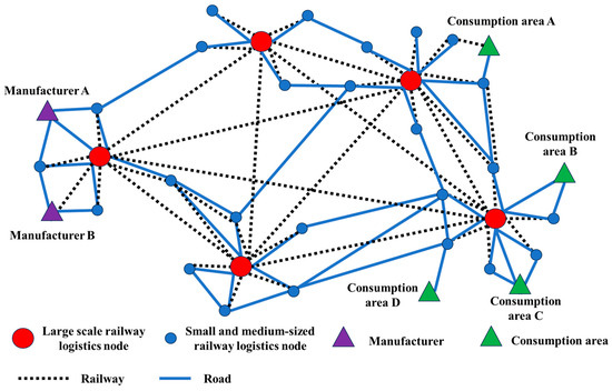
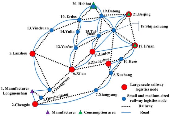
To establish a scientific, efficient, and practical optimization model for railway logistics, it is essential to integrate foundational data collected from the railway warehousing resource management system with robust computational support. This enables coordinated warehousing resources at both the origin and destination of railway trunk line transportation, as well as the successful development of third-party logistics warehousing services. The architecture of the railway logistics service network is illustrated in Figure 1.
Figure 1.
Diagram of railway logistics service network architecture.
In the schematic diagram of the railway logistics network, large and small railway logistics nodes are included, with connections between different nodes via rail, road, or waterway transportation modes. This study focuses on express freight with high timeliness requirements and temporarily excludes waterway transportation. To establish a green railway logistics solution optimization model, the following assumptions are made.
- (1)
- Assuming that the rail and road transport capacities between nodes are unlimited, priority should be given to connecting major nodes through railway transportation mode. This assumption ensures that rail warehousing operations primarily serve the rail trunk line transportation. Mode transitions can only occur at nodes.
- (2)
- Assuming that the storage capacity of large nodes is large and the storage capacity of small nodes is small, when the storage capacity of large nodes and small nodes reaches the set maximum value, they cannot store goods anymore and need to choose other nearby nodes to replace them; if road transportation is used, goods can arrive and depart at any time. If railway transportation is used, fixed time window requirements must be followed.
- (3)
- Assuming that manufacturer A and B (starting points) produce products for consumption areas A, B, C, and D (ending points), the storage duration of goods at each node is determined based on the transportation time window of each batch of goods; the total output is equal to the total demand, meeting the supply–demand balance; the goods of each batch are not transported separately, and there are no damages or accidents during transportation. Each batch of goods is transported using the same logistics network.
- (4)
- Assuming that the goods arrive at the destination before the lower limit of the time window, storage fees need to be paid; if the destination is reached later than the upper limit of the time window, a penalty fee for delayed delivery will be charged; the storage cost of unit goods is lower than the penalty fee for delay.
4.2. Model Construction
Based on the above assumptions, with the goal of minimizing the total cost of carbon emissions and logistics, establish an objective function, and solve the model to obtain the optimal railway logistics solution.
Logistics cost objective function:
Objective function (Formula (5)) represents the total logistics cost from the starting point to the end point (yuan); it contains transportation costs for goods in transit, loading and unloading costs at intermediate nodes, loading and unloading costs at the starting and ending points, storage costs for goods arriving at intermediate nodes before the lower limit of the time window, storage costs for goods arriving at the end point before the lower limit of the time window, and a penalty fee for delay. Formula (6) represents the arrival time of the goods at node using transportation mode . When the node is the starting point, it is the customer’s delivery time. At the intermediate and final nodes, the arrival time is obtained by adding the departure time of the previous node, transportation time and the transit time.
In the formulas, represents the unit transportation cost (yuan/t) of using transportation mode to transport goods from node to node . represents the unit loading and unloading cost (including 1 unloading and 1 loading) of transferring from transportation mode to transportation mode at node (yuan/t). represents the sum of unit loading and unloading costs at the starting node and the destination node (including 1 loading and 1 unloading) (yuan/t). represents the unit storage cost () for goods arriving at the node before the lower limit of the time window. represents the unit penalty cost () for goods arriving at the destination later than the upper limit of the time window. For the transportation batch , represents the departure time of the goods at the starting node ; represents the time when the goods arrive at the node by transportation mode , calculated by Formula (6); represents the time when the goods arrive at the destination node by transportation mode ; represents the departure time from node to node using transportation mode ; represents the time window for the arrival of the goods at the destination ; represents the transportation time (h) for using transportation mode to transport goods from node to node ; represents the transit time (h) for a unit of goods to change transportation modes at node .
Using the standardized weighting method, transform the dual-objective optimization problem into a single-objective optimization problem [24]. Calculate the value of carbon emission cost objective function when the logistics cost is minimized, and calculate the value of logistics cost function when the carbon emission cost is minimized. Then, use and to standardize the carbon emission cost objective and logistics cost objective , respectively, in order to eliminate the difference in magnitude between the two objective functions. Finally, add them together by weighting to obtain the overall objective function of the single-objective optimization model.
Overall objective function:
Constraints:
In the model, objective function (Formula (7)) represents weighted carbon emission costs and logistics costs. represents the weight of carbon emission cost objective function, , and represents the weight of logistics cost objective function, , . Formula (8) represents selecting only one transportation mode between any two nodes. Formula (9) represents that the goods are only transferred once at any node. Formula (10) represents that there is a complete transportation path from the starting node to the destination node . Formula (11) represents the consistency of transportation mode conversion before and after node . Formula (12) represents that the storage capacity of node should be greater than the total amount of goods stored at node at the same time. represents the fuzzy transformation capability constraint of node (). Formula (13) represents that the arrival time of the goods at node should not be later than the upper limit requirement of the goods collection time window at this node. Road transportation can be shipped at any time, but railway transportation needs to be shipped according to the train timetable. Formulas (14) and (15) represent the range of values for decision variables and , with a value of 1 indicating a transportation mode through the specified path is chosen or the goods will change transformation modes at the specified node. Formula (16) represents that the shipment quantity of goods is non-negative. Formula (17) represents that the storage cost for goods arriving earlier than the lower limit of the time window is less than the delay penalty fee for goods arriving later than the upper limit of the time window. This reflects that, if the storage facilities of the railway logistics terminal at the ending point are used instead of the storage and distribution warehouse of the customer enterprise, it can effectively reduce logistics costs while ensuring no shortage of goods. It also reflects the guiding role of market-oriented reform and transformation of railway logistics.
We use triangular fuzzy number to characterize the uncertainty of storage capacity of node [14]. Among them, represents the minimum possible value of capacity, and represents the maximum possible value of capacity, both reflecting two extreme situations where the likelihood of occurrence in practice is extremely low. represents the most likely value of capacity. Therefore, using triangular fuzzy numbers to characterize capability uncertainty can enable logistics solutions to consider various possible scenarios, avoiding overestimation of capability that may lead to infeasible transportation solutions or underestimation of capability that may result in suboptimal transportation solutions.
The uncertainty of capability leads to the uncertainty of planning paths that meet capability constraints. The corresponding real-time capability can only be determined after the actual transportation or replacement operation begins. Once there is a shortage of real-time capability, actual transportation based on planned paths will be interrupted. Therefore, there is a risk of transportation interruption in the logistics solution. Railway logistics enterprises need to combine the risk tolerance attitude of shippers; make balanced decisions between the feasibility, economy, and timeliness of logistics solutions; and ultimately plan the optimal solution that meets customer needs and preferences.
4.3. Model Conversion
The above model contains fuzzy parameters and cannot be directly solved. It is necessary to defuzzify the model, eliminate the fuzzy information in the model, and optimize the solvability of the problem, so as to plan the optimal logistics solution for railway logistics enterprises according to customer needs. We use transformation formula to defuzzify , . is a confidence level parameter.
The membership function of the triangular fuzzy number is defined as:
Then, is defined as . For triangular fuzzy numbers, the is a closed interval .
We can derive the lower limit (left boundary) of the closed interval : , so there is , and the upper limit (right boundary) of the closed interval : , so there is .
Then, there is . When , there is as a support set; when , there is as a core. According to the method of calculating the expected value of , when the confidence level is , the mean of the fuzzy number is [14]. reflects the customer’s risk tolerance level, and the larger the value of , the higher the customer’s tolerance for risk; the smaller the value of , the lower the customer’s tolerance for risk, and the higher the reliability of the logistics solution required.
The parameter of customer’s risk tolerance level comes from the capacity constraints of the railway logistics network. Due to the uncertainty of logistics network capabilities, some logistics solutions may not be feasible in practice. Therefore, for customers with low risk tolerance, it is necessary to require logistics solutions to be executable. In order to ensure the reliability of the plan, it is even possible to choose a suboptimal logistics solution.
Using the defuzzify method of above, transform constraint condition (11) into an equivalent clear form as follows:
4.4. Model Solution
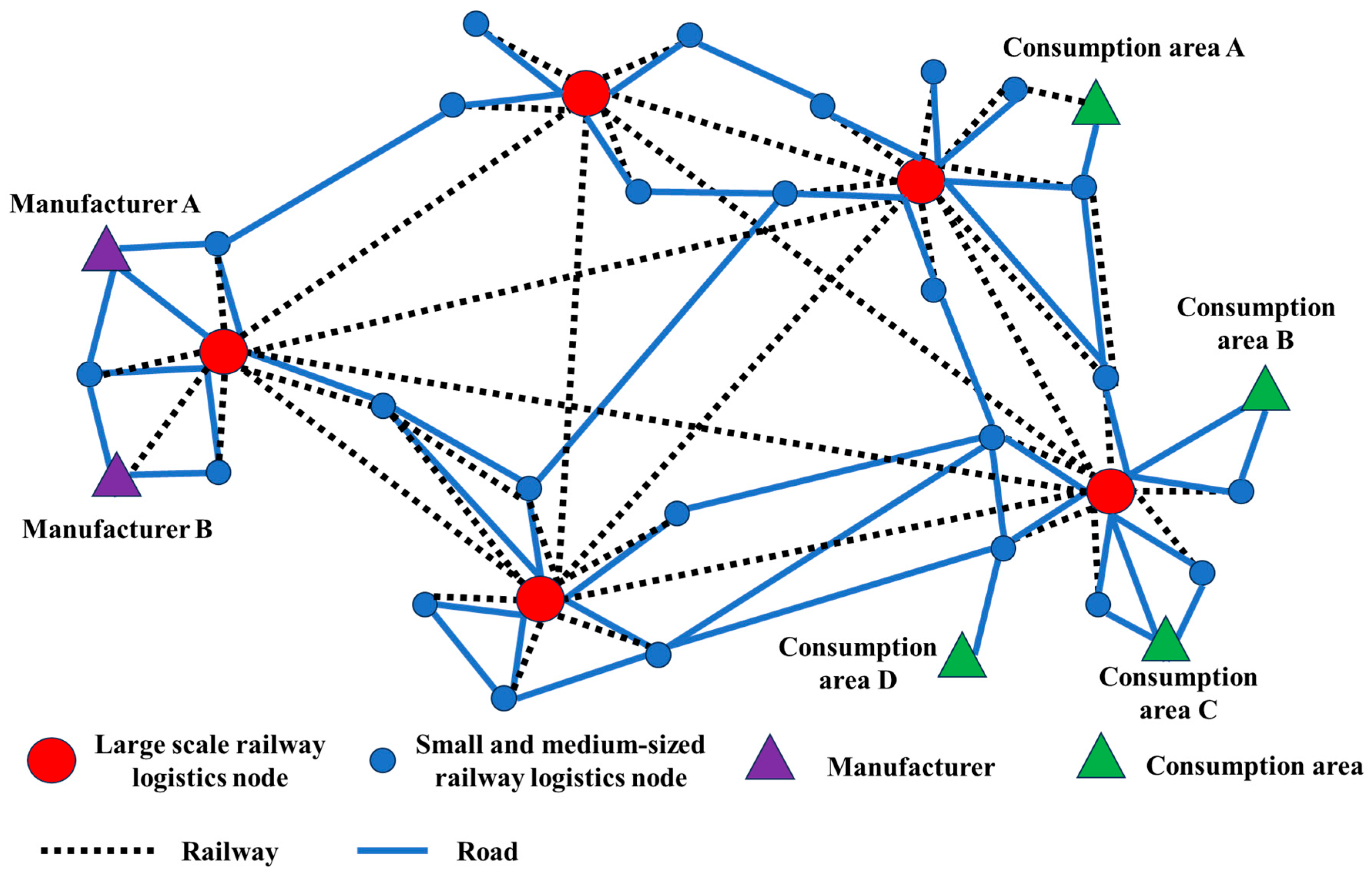
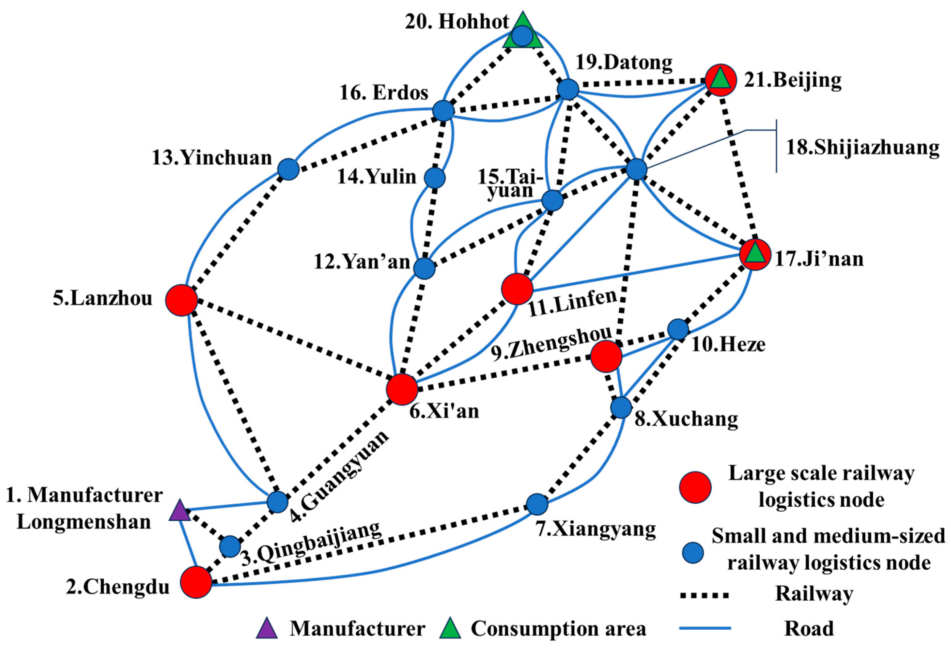
To verify the effectiveness of the model, a network consisting of 21 logistics nodes is constructed, including one manufacturer and three consumption areas. The manufacturer is connected to nearby logistics nodes through road (1-2, 1-4) and railway siding (1-3), while the consumption areas are located on railway logistics nodes 17, 20 and 21. The railway logistics network used for model solving is shown in Figure 2.
Figure 2.
Diagram of model solving network layout.
The logistics network path parameters and the storage costs, storage capacity, and railway goods collection time windows of each node in Figure 2 are shown in Table 1 and Table 2. In network parameter design, the transportation distance between logistics nodes is the actual transportation path length between nodes, which is determined through navigation software AMAP. This model assumes that the transportation distance between highways and railways is the same. The transportation time is calculated based on the speed of road and railway transportation. Considering the significant differences in road transportation costs across different regions, seasons, time periods, types of goods, vehicle models, and wind speed, a relatively reasonable estimate is selected as the parameter for the express freight road transportation cost of this model by consulting the Road Logistics Information Network. At the same time, there are significant differences in railway transportation costs among different railway bureaus, transportation batches, types of railway freight cars, and types of railway logistics services. The parameters of loading and unloading fees and storage fees are estimated based on the current standards for loading and unloading fees at railway logistics terminals. The speed of highway transportation is based on the speed limit of highway trucks, while the speed of railway transportation is assumed to be a fast freight train with a speed of 60 km/h. The values of the model parameters are shown in Table 3.
Table 1.
Logistics network paths parameters.
Table 2.
Logistics network nodes parameters.
Table 3.
Simulation experiment parameter values.
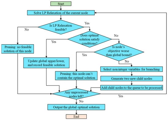
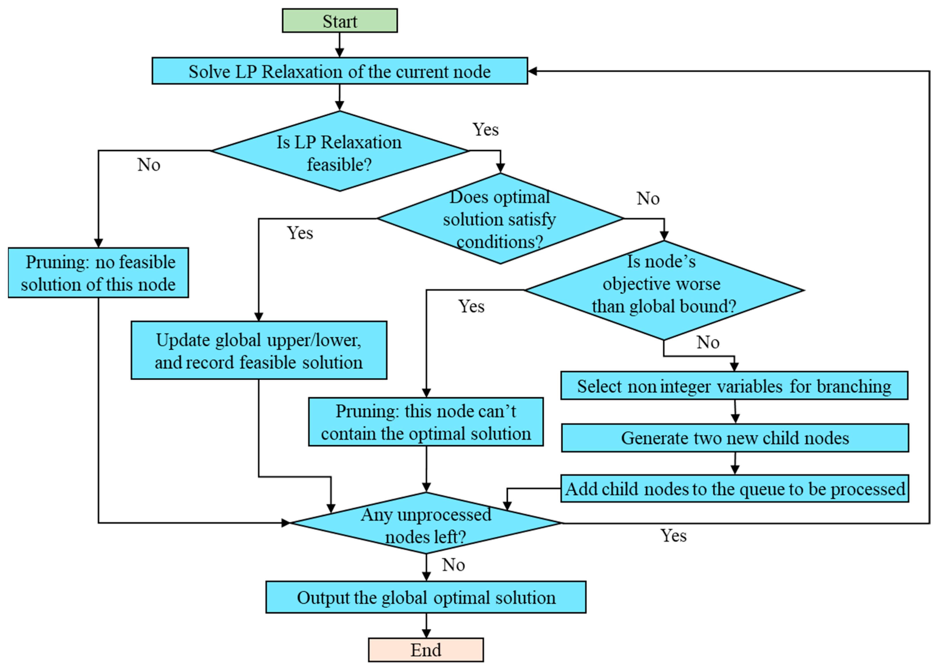
This model incorporates triangular fuzzy numbers and nonlinear constraints. method is used to convert the triangular fuzzy numbers into linear programming forms, and the approach in Reference [21] is adopted to linearize the nonlinear terms in both the objective function and the constraints. Consequently, an integer linear programming (LP) model is obtained. Given the relatively small number of nodes in the case study, it is unnecessary to design a heuristic algorithm for large-scale network problems; instead, the branch-and-bound method implemented in Lingo 21.0 (educational version) can be directly applied to derive the green railway logistics solutions. The solution flowchart of the branch-and-bound method is shown in Figure 3.
Figure 3.
Branch-and-bound solution flowchart.
5. Discussion
Based on the above parameters, we can solve the model in different logistics scenarios and analyze the impact of factors on logistics solutions and total costs, such as delivery time limit, shipment time, multiple batch goods flow, the weights of objective functions, and the customer’s risk tolerance level . To verify the effectiveness of the model, we designed six scenarios for simulation verification. Scenarios 1 to 3 are all single batch cargo transportation in order to verify the impact of time window changes on logistics solutions; Scenario 2 and Scenario 3 are comparative analyses of the impact of customer’s risk tolerance level on logistics solutions. Scenarios 4 to 6 are used to verify the impact of the stacking of multiple batches of goods on logistics solutions. At last, we analyzed the impact of changes in two target weight settings on logistics solutions in Section 5.3.
5.1. Single Batch Goods Logistics Solutions Analysis
Firstly, we analyze the impact of changes in time windows and the customer’s risk tolerance level on logistics solutions during the transportation of a single batch of goods. The weight coefficients are taken as . The customer’s risk tolerance level is taken as or . The reason for choosing value of 0.6 or 0.7 is that, after calculation, is the critical value that affects the logistics solution. Therefore, these two typical values were selected for the case study. The solution results are detailed in Table 4.
Table 4.
Model solution results of single batch goods.
- (1)
- Scenario 1
The goods are transported from node 1 to node 21, with a customer’s shipment quantity of 300 t. The shipment time is 00:00 on the first day, and the arrival time window is the second day [08:00, 11:00]. The total cost is 155,145 yuan, and carbon emission cost is 465 yuan. Compared to Scenario 2, railway transportation is more economical and environmentally friendly than road transportation, but its transportation efficiency is relatively poor. When the delivery time matches the railway transportation schedule, using railway transportation can ensure timely delivery and reduce logistics and carbon emission costs.
- (2)
- Scenario 2
To analyze the impact of delivery time on logistics solutions, based on Scenario 1, the arrival time window is adjusted to the second day [02:00, 05:00], and other parameters remain unchanged. At this time, if railway transportation is used throughout the entire process, the goods will arrive beyond the time window, resulting in a large number of penalty fees. Therefore, the model proposes an intermodal transportation solution by rail and road, with a total cost of 198,519 yuan, including a carbon emission cost of 999 yuan. The addition of road transportation increases the carbon emission cost by 115%. Therefore, from the comparison between Scenario 1 and Scenario 2, it can be seen that setting a reasonable time window and aligning the production plan of the enterprise with the transportation time of the railway logistics enterprise can effectively reduce the total cost.
- (3)
- Scenario 3
To analyze the impact of the customer’s risk tolerance level on logistics solutions, based on Scenario 2, we adjust the value of from 0.7 to 0.6. This means that customers have a reduced risk tolerance level and require more reliable railway logistics solutions. The transformation capacity of small- and medium-sized railway logistics nodes (blue nodes in Figure 2) will decrease to 299 t/d (below 300 t/d); it means that transportation modes cannot be converted at blue nodes. At this time, the logistics solution cannot change transportation modes at node 18, and more road transportation will be used. Therefore, the higher the customer’s risk tolerance level, the more stringent the constraints of railway logistics solutions will be.
5.2. Multiple Batches Goods Logistics Solutions Analysis
Secondly, we analyze the impact of multiple batches of goods transportation on railway logistics solutions, assuming there are three batches of goods starting transportation simultaneously. The first batch of goods is Scenario 1, the second batch of goods is Scenario 4, and the third batch of goods is Scenario 5. The specific parameter settings and solution results are detailed in Table 5.
Table 5.
Model solution results of multiple batches goods.
- (1)
- Scenario 4
The goods are transported from node 1 to node 20, with a customer’s shipment quantity of 300 t. The shipment time is 00:00 on the first day, and the arrival time window is from 21:00 on the first day to 24:00. The recommended solution for the model is the rail and road intermodal transportation plan, with a total cost of 226,386 yuan, including a carbon emission cost of 1806 yuan.
- (2)
- Scenario 5
The goods are transported from node 1 to node 17, with a customer’s shipment quantity of 800 t. The shipment time is 00:00 on the first day, and the arrival time window is from 22:30 on the first day to 01:30 on the second day. The total cost of the recommended solution is 534,016 yuan, including a carbon emission cost of 3776 yuan.
- (3)
- Scenario 6
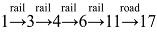
In scenarios 1, 4, and 5, three batches of goods are shipped simultaneously, and the other parameters remain unchanged. Then, there will be a goods flow superposition, as the first batch of goods will be transported by railway throughout the entire process, without being limited by the collection time window and storage capacity of the transfer nodes. However, the second batch of goods (Scenario 4) and the third batch of goods (Scenario 5) need to change transportation modes at node 6, which has a storage capacity of 970 t () and cannot meet the requirements () for simultaneous operations. Previously, we assumed that the goods of each batch were not transported separately, so they could not be split for transportation at node 6. Finally, the second batch of goods arrives at node 6 for transportation first, and then, the logistics solutions for the third batch of goods should be adjusted to 1-rail-3-rail-4-rail-6-rail-11-road-17. It will perform railway to road transformation at node 11 (, when ) to avoid insufficient storage capacity at node 6.
5.3. The Impact of Objective Function Weight on Logistics Solutions
Finally, we analyze the impact of objective function weights on railway logistics solutions. In the previous study, were taken. When the value of changes, the logistics plan results are detailed in Table 6.
Table 6.
Model solution results of weights values change.
The weights change results indicate that the higher the weight of carbon emission costs, the greater the probability of railway transportation being selected in logistics solutions. On the contrary, the lower the weight of carbon emission fees, the greater the probability of road transportation being selected. The results fully demonstrate the positive role of railway transportation in reducing carbon emissions.
6. Conclusions
As a green transportation mode with high capacity, low energy consumption, and intensification, railway freight has a significant responsibility in facilitating the implementation of carbon peak and carbon neutrality strategies. The country has put forward clear requirements for increasing railway freight volume and railways’ share of national freight volume. To further implement national strategies and requirements, railway logistics enterprises deepen the market-oriented reform of logistics, vigorously carry out railway logistics general contracting and full process logistics services, actively promote diversified joint venture and cooperation operations of railway logistics terminals, enrich logistics service content, explore the development of logistics station warehousing services, and provide integrated logistics solution design and comprehensive logistics services for customer enterprises. The research results indicate that:
- (1)
- On the basis of the traditional multimodal transportation path optimization model, further considering factors such as the superposition of multiple batches of goods flows, the storage capacity of railway logistics nodes, the railway transportation time window, and the joint construction of railway warehouses and enterprise warehouses, a green railway logistics solution optimization model is established. Compared with existing research, by setting parameters of our model, it can highlight the basic attributes of railway as a public service resource, ensure the national economy and people’s livelihoods, and has more practical application scenarios. For example, in the parameter settings, we considered the future situation of railway logistics stations providing warehousing services and set conditions for warehousing construction at logistics nodes, and different levels of railway logistics nodes have varying sizes of warehousing capacity.
- (2)
- The simulation results of the model show that the joint construction of customer enterprise production warehouse and railway storage warehouse, replacing the customer distribution center with railway storage facilities, or constructing railway siding can effectively reduce the cost of short-haul transportation and improve the overall logistics efficiency. For example, the railway siding established between node 1 and node 3 can directly transport goods by railway from the enterprise factory to the mainline railway network. Nodes 17, 20, and 21 all use railway storage facilities as customer distribution centers, effectively reducing the short-haul road links after railway transportation and lowering logistics costs.
- (3)
- When customers have strict requirements for the delivery time of logistics services, railway logistics enterprises can use road transportation as necessary to improve the overall transportation efficiency and ensure that the goods can be delivered within the customer’s requested time. The lower the customer’s tolerance for risk, the higher the logistics solution’s requirements for the node’s transportation capacity. We can see from the numerical experiment comparison between Scenario 2 and Scenario 3 the impact of changes in customer’s risk tolerance on railway logistics solutions.
- (4)
- When coordinating the production plan of the customer’s enterprise with the railway transportation time window, other conditions remain unchanged, which can effectively reduce logistics costs and enhance the competitiveness of railway logistics enterprises (Scenario 1 and Scenario 2). In future research, when simulating the national railway logistics network, the model involves a huge computational scale, and more efficient heuristic algorithms need to be designed to improve the speed of model solving in order to achieve rapid updates and real-time response of railway logistics solutions.
Author Contributions
Conceptualization, D.W. and P.Z.; methodology, D.W. and P.Z.; software, D.W.; validation, D.W.; formal analysis, D.W. and P.Z.; investigation, D.W. and C.C.; data curation, D.W.; writing—original draft preparation, D.W. and P.Z.; writing—review and editing, D.W.; supervision, C.C.; funding acquisition, D.W. and C.C. All authors have read and agreed to the published version of the manuscript.
Funding
This study was funded by the science and technology research and development program project of China Railway Group Co., Ltd. no. J2025X001.
Data Availability Statement
All data generated or analyzed during this study are included in this paper.
Conflicts of Interest
Author Danzhu Wang, Pingbiao Zheng and Cheng Chen were employed by China Academy of Railway Sciences Corporate Limited. The authors declare that the research was conducted in the absence of any commercial or financial relationships that could be construed as a potential conflict of interest.
References
- Li, F. Optimization design of short life cycle product logistics supply chain scheme based on support vector machine. Comput. Intell. Neurosci. 2022, 2022, 2311845. [Google Scholar] [CrossRef] [Scilit] [PubMed]
- Hong, J.D.; Judith, L.M. Biofuel logistics network scheme design with combined data envelopment analysis approach. Energy 2020, 209, 118342. [Google Scholar] [CrossRef] [Scilit]
- Sun, Y.; Ge, Y.; Wang, F.; Wang, D. Optimization for a green intermodal routing problem of time-sensitive goods under interval fuzzy demand. J. Railw. Sci. Eng. 2026, 23, 644–654. [Google Scholar]
- Zhu, Y.; Suo, J. The situation of offshore oil logistics industry and transportation scheme design of new concept of green logistics. J. Coast. Res. 2020, 112, 447–450. [Google Scholar] [CrossRef] [Scilit]
- Kabadurmus, O.; Erdogan, M.S. A green vehicle routing problem with multi-depot, multi-tour, heterogeneous fleet and split deliveries: A mathematical model and heuristic approach. J. Comb. Optim. 2023, 45, 89. [Google Scholar] [CrossRef] [Scilit]
- Efthymiadis, S.; Liapis, N.; Nenes, G. Solving a heterogeneous fleet multi-compartment vehicle routing problem: A case study. Int. J. Syst. Sci. Oper. Logist. 2023, 10, 2190474. [Google Scholar] [CrossRef] [Scilit]
- Kim, G. Electric vehicle routing problem with states of charging stations. Sustainability 2024, 16, 3439. [Google Scholar] [CrossRef] [Scilit]
- Huang, R.; Zhao, X.; Wang, J. Optimization of Intermodal Transportation Network Design Considering Demand Uncertainty under the background of ‘Dual Carbon’. J. Transp. Syst. Eng. Inf. Technol. 2025, 42, 41–51. [Google Scholar]
- Hu, Y.; Wu, H.; Jian, W.; Li, Z. Multimodal transport path optimization considering fuzzy demand under mixed time window. Railw. Transp. Econ. 2025, 47, 23–33. [Google Scholar]
- Wu, Y.; Zhang, R. Evaluation model for a port hinterland intermodal freight network considering environmental impacts and capacity constraints. Transp. Res. Rec. J. Transp. Res. Board 2023, 2677, 462−478. [Google Scholar] [CrossRef] [Scilit]
- Chen, W.; Gong, H.; Fang, X. Multimodal transportation route optimization considering transportation carbon tax and quality commitment. J. Railw. Sci. Eng. 2022, 19, 34−41. [Google Scholar]
- Wang, Q.; Li, Y.; Li, H.; Luo, J.; Xian, Y.; Li, P. Research on route optimization of low carbon multimodal transport under uncertainty condition. Railw. Transp. Econ. 2023, 45, 62–69,120. [Google Scholar]
- Yang, Q.; Chen, Z.; Wang, Z.; Deveci, M. A refined two-stage fuzzy hybrid decision making support framework for enhancing logistics and manufacturing integration. Adv. Eng. Inform. 2025, 68, 103780. [Google Scholar] [CrossRef] [Scilit]
- Sun, Y.; Zhang, C.; Chen, A.; Sun, G. Modeling a green and reliable intermodal routing problem for food grain transportation under carbon tax and trading regulations and multi-source uncertainty. Systems 2024, 12, 547. [Google Scholar] [CrossRef] [Scilit]
- Wei, H.; Guo, S. Calculation of carbon emissions of China-Europe container multimodal transport logistics. J. Railw. Sci. Eng. 2025, 22, 3880–3893. [Google Scholar] [CrossRef] [Scilit]
- Jiao, L.; Liu, Y.; Huo, X.; Wu, Y. Transportation carbon emission prediction based on convolutional neural network. Railw. Transp. Econ. 2024, 46, 49–57. [Google Scholar]
- Zhao, R.; Zhao, Y.; Xiong, X.; Tang, Y. Measurement of carbon emission efficiency and analysis of influencing factors in railway transportation enterprise based on Sbm-Malmquist-Tobit model. Railw. Transp. Econ. 2025, 47, 11–23. [Google Scholar]
- Su, H.; Li, H. Route optimization on low-carbon multimodal transport of refrigerated containers under uncertain demand. Railw. Transp. Econ. 2025, 47, 61–69. [Google Scholar]
- Zhou, Y. Research on Carbon Emission System Simulation and Emission Reduction Path of Transportation Industry. Master’s Thesis, Chongqing Jiaotong University, Chongqing, China, 2023. [Google Scholar]
- Wu, M. Analysis of fuel consumption limits and measurement methods for operating trucks. Highw. Automot. Appl. 2010, 05, 25–29. [Google Scholar]
- Wu, B.; Zhang, H.; Pang, R.; Zhang, P. Multi-scenario analysis of carbon emissions from highway transportation in Heilongjiang Province. J. Saf. Environ. 2025, 25, 4874–4887. [Google Scholar]
- Ma, J.; Gao, Z.; Shang, L.; Liu, H.; Zhang, T. Calculation model for generalized carbon emission costs of typical logistics enterprises. Railw. Transp. Econ. 2025, 47, 95–104. [Google Scholar]
- Global Logistics Emissions Council. Global Logistics Emissions Council Framework V3.0; Smart Freight Centre: Amsterdam, The Netherlands, 2023. [Google Scholar]
- Sun, Y.; Yu, N.; Wang, D.; Chen, W. Study on the bi-objective optimization for the multimodal routing problem with multiple time windows. Railw. Transp. Econ. 2021, 43, 82–89. [Google Scholar]
- Chen, Y.; Xiao, R.; Huang, W.; Luo, Y.; Zhang, M. Railway and highway freight rate comparison for modern logistics competition. Railw. Logist. 2025, 43, 19–24. [Google Scholar]













Disclaimer/Publisher’s Note: The statements, opinions and data contained in all publications are solely those of the individual author(s) and contributor(s) and not of MDPI and/or the editor(s). MDPI and/or the editor(s) disclaim responsibility for any injury to people or property resulting from any ideas, methods, instructions or products referred to in the content. |
© 2026 by the authors. Published by MDPI on behalf of the International Institute of Knowledge Innovation and Invention. Licensee MDPI, Basel, Switzerland. This article is an open access article distributed under the terms and conditions of the Creative Commons Attribution (CC BY) license.