Uncertainty-Aware Continual TinyML Driver Fatigue Detection with Kolmogorov–Arnold Networks at the IoT Edge

Abstract

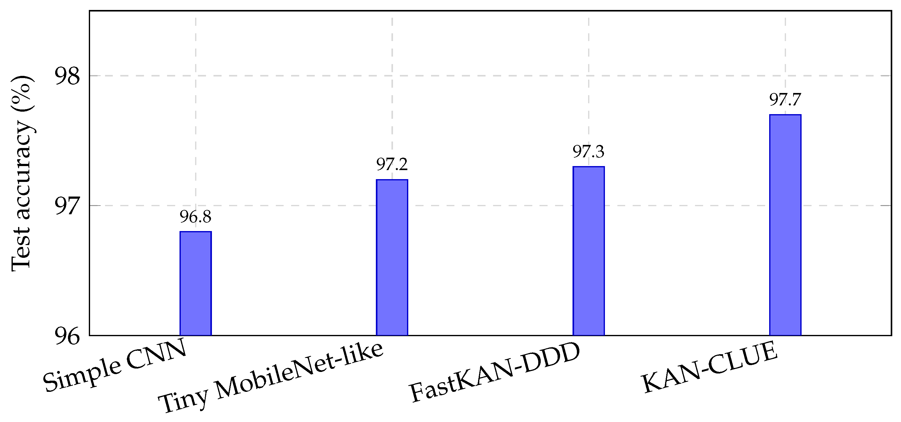
Driver fatigue is a major cause of road accidents, and in-cabin monitoring is increasingly embedded into the Internet-of-Things (IoT) ecosystem of modern vehicles. Deploying such monitoring directly on microcontroller-class devices is challenging: models must fit tight memory and compute budgets, provide reliable confidence estimates, and adapt online to new drivers and conditions. We propose KAN-CLUE, an uncertainty-aware continual TinyML framework for driver fatigue detection from near-infrared periocular images at the IoT edge. KAN-CLUE combines a compact convolutional backbone with a Kolmogorov–Arnold Network (KAN) classification head that outputs Dirichlet-distributed class probabilities and a principled predictive uncertainty measure. A lightweight activation-histogram mechanism provides an additional out-of-distribution (OOD) score, and both signals drive an on-device continual learning scheme that selectively updates a small subset of parameters under a KAN-specific EWC-style regularization. On the ULg DROZY drowsiness database, the quantized KAN-CLUE model uses roughly 167k parameters (about 165 kB in Flash), requires on the order of ${10}^6$ MACs, and achieves around 3.1 ms latency on a Cortex-M–class microcontroller, while reaching 97.7% test accuracy with improved calibration and OOD detection compared with softmax-based TinyML baselines.

1. Introduction

Road traffic accidents remain a leading cause of injury and mortality worldwide, and driver fatigue has been consistently identified as a critical risk factor in both highway and urban driving scenarios [1]. Fatigued drivers exhibit slower reaction times, impaired decision-making, and reduced situational awareness, which can easily lead to lane departures, delayed braking, or failure to perceive hazards [2]. As modern vehicles increasingly adopt advanced driver assistance systems (ADAS) and in-cabin sensing technologies, there is a strong demand for reliable, low-cost, and privacy-preserving driver fatigue monitoring solutions that operate continuously and unobtrusively [3].

Vision-based methods that analyze facial cues such as eye closure, blinking, yawning, and head pose have shown considerable promise for contactless fatigue monitoring in realistic conditions [4]. Recent work has explored a variety of deep architectures, including dense multi-pooling convolutional networks, attention-based fusion of local and global facial regions, and object-detection-based pipelines built on YOLO variants, often augmented with temporal modeling to capture fatigue dynamics over time [5]. These methods can achieve high accuracy on benchmark datasets and even real-time performance on embedded processors. However, most existing solutions either rely on relatively heavy models that are difficult to deploy on microcontrollers, or they are designed as static classifiers that do not adapt to new drivers, environments, or cameras once trained [6].

At the same time, Tiny Machine Learning (TinyML) [7] has emerged as a promising paradigm for executing deep learning models directly on resource-constrained microcontrollers, enabling low-latency inference with reduced energy consumption and without continuous connectivity to remote servers [8]. TinyML is particularly attractive for in-vehicle driver monitoring, where privacy and robustness to network failures are important. Nevertheless, bringing driver fatigue detection to TinyML devices introduces significant challenges: the model must fit within tight memory and compute budgets, retain sufficient representational capacity to capture subtle fatigue-related cues, and ideally expose mechanisms for online adaptation and reliability estimation [9]. Existing TinyML deployments for fatigue or vigilance monitoring, for example using hand-crafted features and shallow neural networks on microcontrollers, typically trade off accuracy and flexibility to satisfy these constraints [10,11,12,13].

Kolmogorov–Arnold Networks (KANs) have recently been proposed as an alternative neural architecture that replaces standard linear neurons with learnable univariate functions organized according to the Kolmogorov–Arnold representation theorem [14]. By learning these univariate spline-based functions, KANs can achieve strong expressivity with a relatively small number of parameters and offer an interpretable structure in which each edge corresponds to a one-dimensional transformation [15]. These properties make KANs an appealing candidate for TinyML deployment, as they may provide a better trade-off between model size and representation power compared with traditional multi-layer perceptrons.

Another crucial aspect in safety-critical applications such as fatigue monitoring is the ability of the model to recognize when it is uncertain. Standard deep networks often produce overconfident predictions even for OOD inputs or highly ambiguous samples, which can be particularly dangerous when the system is used to trigger warnings or interventions [16]. Uncertainty quantification techniques such as ensembles, Monte Carlo dropout, or Bayesian neural networks can address this issue [17], but they generally incur substantial memory and computational overhead that is incompatible with TinyML hardware. Moreover, most existing driver fatigue detection systems do not incorporate uncertainty estimates into their decision logic, nor do they use uncertainty to drive online adaptation or active learning [18].

Motivated by these gaps, we propose KAN-CLUE, an uncertainty-aware continual-learning TinyML framework with Kolmogorov–Arnold Networks for driver fatigue detection. KAN-CLUE targets in-vehicle near-infrared camera setups similar to those captured in the ULg Multimodality Drowsiness Database (DROZY), which provides synchronized facial recordings and physiological signals under controlled sleep-deprivation protocols. Our framework combines a compact convolutional feature extractor with a KAN-based classification head tailored to microcontroller deployment, and augments this backbone with an evidential output layer and a lightweight continual learning mechanism that adapts the model on-device in response to changing conditions.

The main contributions of this work can be summarized as follows:

• We design a TinyML-ready convolutional–KAN architecture for driver fatigue detection that fits within the memory and compute budgets of microcontroller-class devices while preserving competitive recognition performance on DROZY.
• We introduce an evidential KAN classification head that outputs Dirichlet-distributed class probabilities and a principled predictive uncertainty measure, avoiding the overhead of ensemble- or sampling-based methods.
• We develop an uncertainty-aware continual learning strategy that uses uncertainty and OOD scores to select informative samples for on-device adaptation, while a regularization term anchored on KAN parameters mitigates catastrophic forgetting and maintains performance on previously seen conditions.
• We provide a comprehensive experimental evaluation on DROZY, including comparisons with TinyML-compatible baselines and ablation studies that quantify the effect of uncertainty estimation and continual learning on accuracy, calibration, and resource usage.

The remainder of the paper is organized as follows. Section 2 reviews related work on driver fatigue detection using visual, physiological, and multimodal data. Section 3 details the proposed KAN-CLUE framework, including the data preprocessing pipeline, TinyML model architecture, uncertainty quantification scheme, and continual learning mechanism. Section 4 describes the embedded experimental setup, and Section 5 reports and analyzes the empirical results. Section 6 discusses the implications and limitations of our findings, and outlines directions for future work. Section 7 concludes the paper.

2. Related Works

We review recent advances in driver fatigue detection along three complementary directions: vision-based methods, physiological-signal-based approaches, and multimodal frameworks that fuse visual and physiological data for improved robustness in realistic driving scenarios.

2.1. Driver Fatigue Detection Using Visual Data

Vision-based methods typically analyze facial cues and spatio-temporal patterns from images or video sequences, aiming for robustness and real-time performance. Han et al. [19] proposed DMP-Net, a dense multi-pooling CNN pipeline that detects eye and mouth states and infers fatigue using PERCLOS and mouth-opening frequency, achieving above 99% accuracy on CEW, ZJU, and a self-collected dataset in real time. Zhang et al. [20] introduced MRA-FD, which combines global and local facial regions, attention-based fusion, and a bidirectional LSTM to model temporal dynamics, reaching around 90–94% accuracy on Nthu-DDD and YawDD with real-time feasibility on a Raspberry Pi. Liang et al. [21] further enhanced robustness to pose and visually similar behaviors via multi-granularity facial features, compact spatial fusion, and an LSTM-based temporal network, achieving state-of-the-art performance on NTHU-DDD. In parallel, Li et al. [22] proposed ES-YOLO, an improved YOLOv7 with CBAM attention and Focal-EIOU loss, attaining around 99% mAP on CEW and a self-made dataset while supporting real-time eye-state-based fatigue alarms. Peng et al. [23] adapted YOLOv5 with deformable convolutions, triplet attention, and Wing loss to handle challenging mountain road environments, reaching about 85% average accuracy on WIDERFACE+YawDD plus custom data.

2.2. Driver Fatigue Detection Using Physiological Signals

Physiological-signal-based methods leverage EEG, ECG/HRV, and other biosignals to capture internal fatigue-related changes and enhance cross-subject robustness. Guo et al. [24] proposed MMA-Net, a multi-modality attention network that fuses frontal EEG, EDA, and PPG via signal-adaptive coding and attention-based feature fusion, achieving accuracies above 82% on simulated driving data with Karolinska Sleepiness Scale labels. Lin et al. [13] focused on wearable-friendly HRV-based detection from single-lead ECG, extracting HRV features and training several classifiers; the best BPNN reached 94.35% accuracy and was deployed on an STM32 microcontroller, demonstrating low-cost embedded feasibility. For EEG representation learning, Yang et al. [25] designed adMBCNN, an adaptive multi-branch CNN that jointly exploits handcrafted features (entropy and spectral measures) and functional brain networks, achieving state-of-the-art performance on SEED-VIG and Cui. Addressing cross-subject generalization, Huang et al. [26] introduced a multi-level domain adaptation algorithm combining improved Wasserstein distance and intra-domain contrastive discrepancy, obtaining average semi-supervised accuracies of 94.2% and 84.3% on SEED-VIG and SADT. In a noisy industrial context, Chen and Wang [27] developed CEMD-MACNN, which first denoises EEG via conditional EMD and then applies a multi-scale attention CNN, reaching 98.70% accuracy for tower crane operators and demonstrating strong anti-noise capability.

2.3. Driver Fatigue Detection Using Physiological and Visual Data

Multimodal approaches combine physiological signals and visual cues to improve reliability under realistic operating conditions. Wu et al. [28] evaluated urban railway transit drivers using psychological tests, heart rate and electrodermal activity from wearables, and eye-movement recordings, showing that fused multi-feature machine-learning models yield the best fatigue detection accuracy, especially with longer analysis windows. Cao et al. [29] proposed optimized multimodal neural networks that fuse facial features (ResNet18) with physiological time-series (LSTM on EEG, ECG, EMG, EOG) from DROZY; their feature-coupled model achieved around 98.4% accuracy and F1-score, significantly outperforming simple feature concatenation. Peng et al. [30] presented an end-to-end multi-source fusion network that jointly learns from physiological signals and facial images, avoiding hand-crafted features and obtaining 93.15% detection accuracy within a 3-s window on data from 21 participants, with good specificity and sensitivity and interpretable facial-region visualizations.

2.4. TinyML Deployment, KAN Models, Uncertainty Estimation, and Continual Adaptation

The preceding subsections organized the literature primarily by sensing modality, which is important for understanding how driver fatigue can be inferred from visual, physiological, or multimodal evidence. However, the present work is also positioned along four methodological axes that are central to its design: TinyML deployment, KANs, uncertainty/OOD estimation, and continual adaptation. These aspects are reviewed here explicitly in order to better situate the contribution of KAN-CLUE.

2.4.1. Tinyml-Oriented Fatigue Detection

TinyML has become an increasingly relevant paradigm for driver monitoring because it enables inference directly on microcontroller-class hardware, thereby reducing latency, energy consumption, and dependence on cloud connectivity [7,8]. This is particularly attractive for in-vehicle fatigue monitoring, where privacy, robustness to network loss, and always-on availability are important. Existing TinyML-oriented fatigue and vigilance systems have typically relied on lightweight CNNs, hand-crafted features combined with shallow classifiers, or aggressively quantized compact models [10,11,12,13]. These studies demonstrate that embedded fatigue detection is feasible, but they also reveal a recurring limitation: most deployed TinyML systems remain static after training, expose limited reliability information, and often sacrifice flexibility or uncertainty awareness in order to meet the hardware budget.

2.4.2. Kans and Lightweight Kan-Based Models

Recent work on KANs has suggested that KANs can serve as an attractive alternative to conventional dense heads by replacing fixed scalar activations with learnable univariate functions. This structure can improve expressivity while keeping the model relatively compact, and it also provides a more interpretable parameterization in which each edge corresponds to a one-dimensional nonlinear transformation. General KAN studies and surveys have highlighted their promise for efficient learning and their potential suitability for compressed or resource-aware architectures [14,15]. More directly relevant to fatigue monitoring, FastKAN-DDD showed that a FastKAN-style design can be adapted to driver drowsiness detection under TinyML constraints, achieving strong efficiency and accuracy on a real drowsiness benchmark [10]. These studies establish KANs as a promising ingredient for embedded driver-monitoring systems, but they do not yet address the broader combination of KAN efficiency, uncertainty-aware decision making, and on-device continual adaptation considered in the present work.

2.4.3. Uncertainty and Out-of-Distribution Awareness in Fatigue Monitoring

For safety-critical systems such as driver fatigue detection, accuracy alone is not sufficient. A deployable model should also indicate when its prediction is unreliable, ambiguous, or inconsistent with the training distribution. In the broader machine-learning literature, uncertainty quantification has been studied through Bayesian neural networks, Monte Carlo dropout, ensembles, and evidential formulations [16,17]. These approaches can improve calibration and help flag OOD inputs, but many of them incur significant memory or runtime overhead that is poorly matched to TinyML hardware. At the application level, most existing fatigue-detection systems still operate as deterministic classifiers and do not use predictive uncertainty as a first-class signal for decision logic or adaptation [6,18]. This leaves a practical gap between the needs of trustworthy in-vehicle monitoring and the capabilities of current embedded fatigue detectors.

2.4.4. Continual Adaptation at the Edge

A further challenge is that driver-monitoring systems are exposed to gradual and recurrent distribution shifts. Changes in driver physiology, facial appearance, camera placement, illumination, sensor noise, or operating environment can all degrade a model that was trained once and then frozen. In practice, however, most fatigue-detection pipelines reported in the literature remain static after offline training, even when they are deployed on edge devices. This means that there is still limited work on continual learning for TinyML driver fatigue detection, and even less on continual learning that is explicitly guided by calibrated uncertainty and OOD signals. This issue is particularly important in embedded driver monitoring because adaptation capacity is constrained by tight memory, compute, and energy budgets.

2.4.5. Positioning of the Present Work

Against this background, KAN-CLUE is designed to occupy a different point in the literature landscape. Rather than focusing only on the sensing modality or only on compact inference, it combines four properties in a single TinyML-ready framework: a compact vision backbone for embedded deployment, a KAN-based classification head, principled uncertainty/OOD estimation, and a lightweight continual learning mechanism for controlled on-device adaptation. In this sense, the contribution is not merely another visual fatigue detector, but a step toward trustworthy and adaptive TinyML fatigue monitoring at the IoT edge (see

Table 1. Methodological positioning of representative prior work relative to the four design axes emphasized in this paper.

Representative Line of Work	TinyML-Ready	KAN-Based	Uncertainty/OOD	Continual Adaptation
Visual, physiological, and multimodal fatigue detectors [19,24,28,29,30]	Partial	No	No	No
Embedded/TinyML fatigue detectors [10,11,12,13]	Yes	No	No	No
General KAN studies and surveys [14,15]	Partial	Yes	No	No
FastKAN-DDD for TinyML drowsiness detection [13]	Yes	Yes	No	No
KAN-CLUE (this work)	Yes	Yes	Yes	Yes

).

Table 2. Summary of related works on driver fatigue detection.

Approach	Ref.	Model	Dataset	Performance	TinyML Model
Vision-based	[19]	DMP-Net + PERCLOS	CEW, ZJU, self-collected	Acc.: 99.25% (CEW), 99.24% (ZJU), 99.12% (self); 3.5 ms/frame
	[20]	MRA-FD: MTCNN + Feature Attention + BiLSTM + IsoSSL-MoCo	NTHU-DDD, YawDD	Acc.: 90.10% (NTHU-DDD), 94.37% (YawDD)
	[21]	FMIF: multi-granularity facial fusion + LSTM temporal modeling	NTHU-DDD	Outstanding performance vs existing approaches (value not specified)
	[22]	ES-YOLO: improved YOLOv7 + CBAM + Focal-EIOU	CEW, self-made	mAP: 99.0% (CEW), 98.8% (self)
	[23]	Improved YOLOv5 + DCN + Triplet Attention + Wing loss	WIDERFACE + YawDD + mountain-road images	Avg. accuracy: 85%
Physiological	[24]	MMA-Net: 1D-CNN + LSTM + attention fusion	28-subject simulated dataset (KSS labels)	Acc.: up to 82.14%; F1: 82.61%
	[13]	BPNN	18-subject simulated ECG dataset	Acc.: 94.35%
	[25]	adMBCNN: multi-branch CNN + handcrafted EEG feats + brain networks	SEED-VIG, Cui	SOTA reported (values not specified)
	[26]	Dual-level domain adaptation (Wasserstein + contrastive discrepancy)	SEED-VIG, SADT	Cross-subject Acc.: 94.2% and 84.3% (semi-supervised)
	[27]	CEMD-MACNN for noisy EEG (tower crane drivers)	Self-collected (10 operators)	Avg. Acc.: 98.70%
Hybrid	[28]	Multi-feature ML fusion (psychological + wearable + camera)	25 professional transit drivers (simulation)	Best performance with fused inputs and longer windows (no value stated)
	[29]	Multimodal NN: ResNet18 (face) + LSTM; feature-coupled model	DROZY	Acc.: 98.41%; Prec.: 98.38%; Rec.: 98.39%; F1: 98.38%
	[30]	End-to-end multi-source fusion NN (physio + facial video)	21 participants (simulated)	Acc.: 93.15% (3s window); Spec.: 94.04%; Sens.: 91.71%
	Ours	KAN-CLUE: Tiny CNN + KANs (evidential)	DROZY	Acc.: 97.7% (test); F1: 0.976; ECE: 0.015; Latency: 3.1 ms/frame; Params: 167k

summarizes these studies by approach category, model type, dataset, performance, and whether TinyML-oriented deployment is considered.

3. Proposed Methodology

3.1. Data Description

In this work, we used the ULg Multimodality Drowsiness Database (DROZY) [31], which was introduced to facilitate the development of robust drowsiness monitoring systems, especially with contactless camera-based sensing in transportation contexts. The dataset is explicitly designed to support research on drowsiness and related operator states by providing synchronized multi-sensor recordings centered on facial analysis and physiology. It combines remote sensing with classical sleepiness/vigilance assessment tools, making it suitable for both vision-based and physiology-inspired modeling.

The data were collected from 14 healthy participants (3 males and 11 females), with a mean age of approximately 22.7 years. The protocol aimed to induce increasing levels of sleep deprivation across two consecutive days. Each subject performed three Psychomotor Vigilance Tests (PVTs) under controlled laboratory conditions, progressing from a well-rested state to acute sleep deprivation. Participants were required to follow a normal sleep routine prior to the first test and then remain awake until the third PVT, resulting in roughly 28–30 h of total sleep deprivation. The study environment was carefully controlled (e.g., reduced external stimuli and limited prior screen exposure), and the Karolinska Sleepiness Scale (KSS) self-assessment was recorded before each PVT to provide a subjective estimate of drowsiness.

A key strength of DROZY is its multimodality and strict temporal synchronization. For each subject and each of the three PVT sessions, the database provides four major categories of data: (1) KSS scores, (2) PVT event markers and reaction times, (3) polysomnography (PSG) signals, and (iv) facial recordings captured by a Microsoft Kinect v2 sensor. The PSG includes five EEG channels, two EOG channels, ECG, and EMG, offering an objective physiological reference for sleepiness-related changes. The Kinect v2 provides near-infrared (NIR) intensity and range facial images, enabling analysis that is robust to lighting variations; these modalities are well aligned with the database motivation of contactless in-vehicle-like monitoring. Additionally, the dataset offers 68 facial landmarks with both 2D image coordinates and 3D camera-space coordinates, obtained via a combination of manual annotations on selected frames and automatic tracking across all frames.

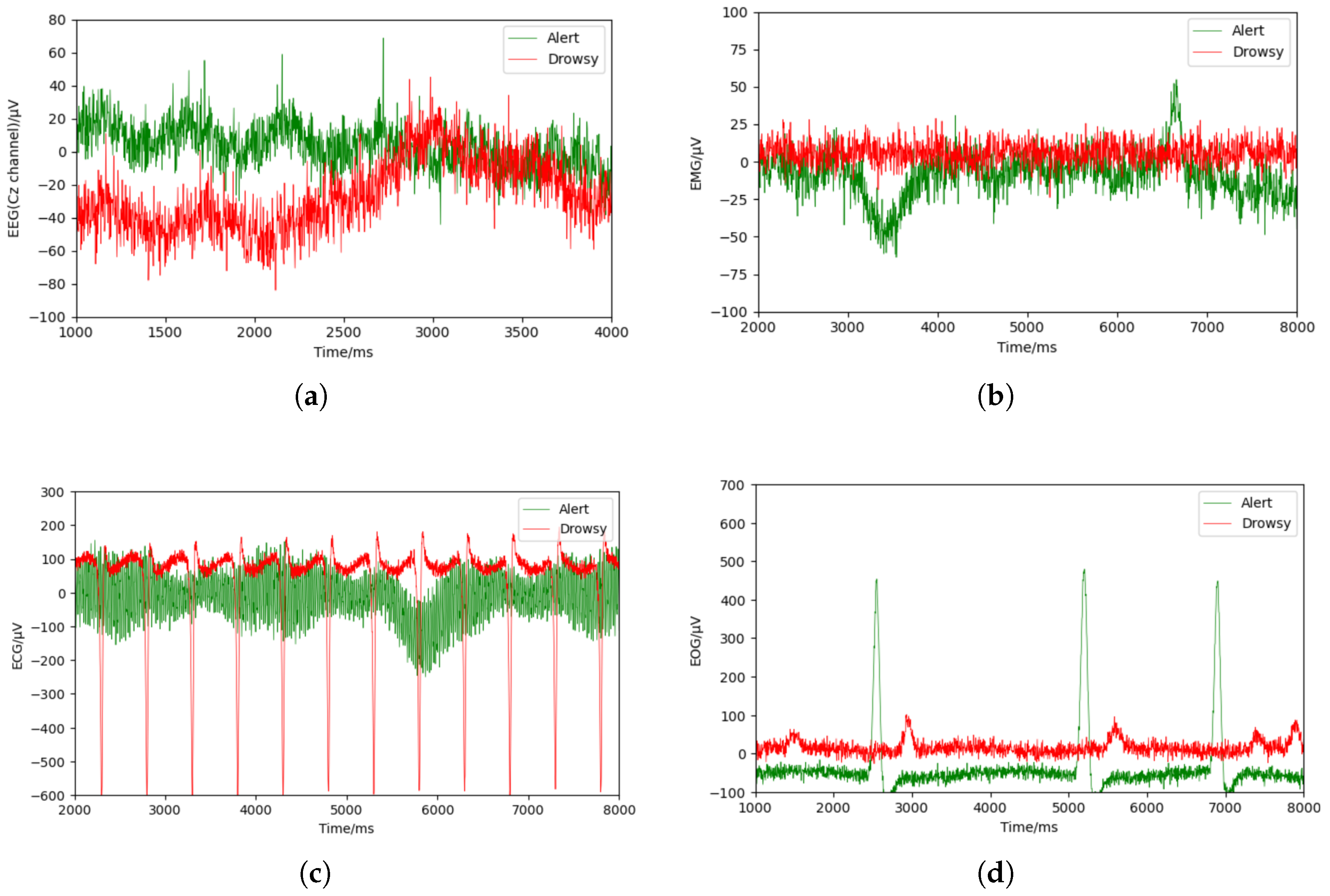
In terms of scale, DROZY contains approximately 500,000 frames of facial data and a total data volume of about 283 GB. This size reflects the richness of the synchronized recordings and the inclusion of both image and physiological streams. The dataset structure supports several experimental directions, such as estimating level of drowsiness from PSG, extracting ocular or facial-behavioral indicators from NIR images, and studying the relationship between visual fatigue cues and objective vigilance outcomes derived from PVT reaction times. Figure 1 presents representative segments of four physiological modalities EEG (Cz channel), EMG, ECG, and EOG. Each comparing the Alert and Drowsy states over time; across these signals, the drowsy condition generally shows more pronounced baseline shifts and transient events, while the alert condition tends to exhibit more regular dynamics, illustrating that vigilance changes can be captured through complementary neural, muscular, cardiac, and ocular patterns.

3.2. Data Pre-Processing

The raw input to the proposed KAN-CLUE framework consists of near-infrared (NIR) facial recordings and associated drowsiness annotations provided by the DROZY database. Before these signals can be used to train and evaluate the TinyML model, they must be transformed into a consistent, compact, and well-labeled representation. The pre-processing pipeline is designed not only to prepare the data from a machine learning perspective, but also to respect the constraints of TinyML deployment on microcontrollers, namely limited memory, limited computational power, and the need for stable and well-normalized inputs.

3.2.1. Temporal Alignment and Frame Selection

Let $s\in \mathcal{S}$ denote the index of a subject in the database. For each subject s, the NIR facial recording can be represented as a sequence of frames $V^{\left(s\right)}\left(t\right)$, with $t=1,2,\dots ,T^{\left(s\right)}$, where $T^{\left(s\right)}$ is the total number of frames in the recording for that subject. The raw recording includes initialization periods, rest phases, and the active Psychomotor Vigilance Test (PVT) interval. The drowsiness analysis is only meaningful within the experimentally defined PVT interval and potentially in its immediate neighborhood.

Using the session metadata or synchronization markers, we determine the frame indices corresponding to the beginning and end of the valid PVT interval for subject s, denoted by $t_{\mathrm{start}}^{\left(s\right)}$ and $t_{\mathrm{end}}^{\left(s\right)}$, respectively. We then define a binary selection mask $m^{\left(s\right)}\left(t\right)$ such that $m^{\left(s\right)}\left(t\right)=1$ if $t_{\mathrm{start}}^{\left(s\right)}\le t\le t_{\mathrm{end}}^{\left(s\right)}$, and $m^{\left(s\right)}\left(t\right)=0$ otherwise, which identifies frames that belong to the valid experimental interval. The set of valid frame indices for subject s is then given by ${\mathcal{T}}^{\left(s\right)}=\left\{t|m^{\left(s\right)}\left(t\right)=1\right\}$. Only frames $V^{\left(s\right)}\left(t\right)$ with $t\in {\mathcal{T}}^{\left(s\right)}$ are retained for subsequent stages. If necessary, a temporal subsampling factor can be applied to reduce redundancy, for example by keeping one frame every k frames, which lowers storage and computational costs and is consistent with TinyML constraints.

3.2.2. Face and Eye Region Localization

After temporal selection, the next goal is to spatially localize the most informative part of each frame for fatigue detection. In vision-based driver monitoring, the face and especially the periocular (eye) region are highly indicative of drowsiness, as they capture blink patterns, eyelid closure, and other fatigue-related cues.

For each valid frame $V^{\left(s\right)}\left(t\right)$ with $t\in {\mathcal{T}}^{\left(s\right)}$, we assume the availability of a set of two-dimensional facial landmarks ${\mathbf{L}}^{\left(s\right)}\left(t\right)\in {\mathbb{R}}^{K\times 2}$, where K denotes the number of landmarks. The k-th landmark is written as ${\mathbf{L}}_k^{\left(s\right)}\left(t\right)=\left(x_k^{\left(s\right)}\left(t\right),y_k^{\left(s\right)}\left(t\right)\right)$, with $x_k^{\left(s\right)}\left(t\right)$ and $y_k^{\left(s\right)}\left(t\right)$ giving its horizontal and vertical coordinates in pixel units. These landmarks may be provided by the database or estimated using a robust facial landmark detector applied to each frame.

A global face bounding box $B_{\mathrm{face}}^{\left(s\right)}\left(t\right)$ is defined as the smallest axis-aligned rectangle that contains all landmarks, namely $B_{\mathrm{face}}^{\left(s\right)}\left(t\right)=\left[x_{\min }^{\left(s\right)}\left(t\right),x_{\max }^{\left(s\right)}\left(t\right),y_{\min }^{\left(s\right)}\left(t\right),y_{\max }^{\left(s\right)}\left(t\right)\right]$, where $x_{\min }^{\left(s\right)}\left(t\right)={\min }_k{x}_k^{\left(s\right)}\left(t\right)$, $x_{\max }^{\left(s\right)}\left(t\right)={\max }_k{x}_k^{\left(s\right)}\left(t\right)$, $y_{\min }^{\left(s\right)}\left(t\right)={\min }_k{y}_k^{\left(s\right)}\left(t\right)$, and $y_{\max }^{\left(s\right)}\left(t\right)={\max }_k{y}_k^{\left(s\right)}\left(t\right)$. To avoid truncating facial regions due to small landmark inaccuracies, this bounding box can be enlarged by a fixed margin $\Delta >0$ on all sides, resulting in an expanded box ${\tilde{B}}_{\mathrm{face}}^{\left(s\right)}\left(t\right)=\left[x_{\min }^{\left(s\right)}\left(t\right)-\Delta ,x_{\max }^{\left(s\right)}\left(t\right)+\Delta ,y_{\min }^{\left(s\right)}\left(t\right)-\Delta ,y_{\max }^{\left(s\right)}\left(t\right)+\Delta \right]$.

In addition to the global face region, the periocular area is often particularly informative for fatigue monitoring. Let ${\mathcal{K}}_{\mathrm{eye}}\subset \{1,\dots ,K\}$ denote the indices of landmarks corresponding to the left and right eyes. The eye bounding box $B_{\mathrm{eye}}^{\left(s\right)}\left(t\right)$ is defined in terms of these landmarks as $B_{\mathrm{eye}}^{\left(s\right)}\left(t\right)=\left[x_{\min ,\mathrm{eye}}^{\left(s\right)}\left(t\right),x_{\max ,\mathrm{eye}}^{\left(s\right)}\left(t\right),y_{\min ,\mathrm{eye}}^{\left(s\right)}\left(t\right),y_{\max ,\mathrm{eye}}^{\left(s\right)}\left(t\right)\right]$, with $x_{\min ,\mathrm{eye}}^{\left(s\right)}\left(t\right)={\min }_{k\in {\mathcal{K}}_{\mathrm{eye}}}{x}_k^{\left(s\right)}\left(t\right)$, $x_{\max ,\mathrm{eye}}^{\left(s\right)}\left(t\right)={\max }_{k\in {\mathcal{K}}_{\mathrm{eye}}}{x}_k^{\left(s\right)}\left(t\right)$, $y_{\min ,\mathrm{eye}}^{\left(s\right)}\left(t\right)={\min }_{k\in {\mathcal{K}}_{\mathrm{eye}}}{y}_k^{\left(s\right)}\left(t\right)$, and $y_{\max ,\mathrm{eye}}^{\left(s\right)}\left(t\right)={\max }_{k\in {\mathcal{K}}_{\mathrm{eye}}}{y}_k^{\left(s\right)}\left(t\right)$. A small padding margin ${\Delta }_{\mathrm{eye}}$ may also be added to this box to include surrounding context such as eyebrows and upper cheeks, which further stabilizes the appearance of the region.

Given a selected bounding box $B^{\left(s\right)}\left(t\right)$, either for the face or for the eye region, a cropping operator $\mathcal{C}(·)$ is applied to extract the corresponding region of interest from the full frame. The cropped image is defined as $I^{\left(s\right)}\left(t\right)=\mathcal{C}\left(V^{\left(s\right)}\left(t\right),B^{\left(s\right)}\left(t\right)\right)$, where $I^{\left(s\right)}\left(t\right)\in {\mathbb{R}}^{H_0\times W_0}$ denotes the raw ROI image at its original spatial resolution $(H_0,W_0)$. In practice, short gaps in landmark detection may arise due to occlusions or motion blur. To avoid discarding all such frames, the last valid bounding box can be propagated forward over a small temporal horizon, under the assumption that head motion is relatively smooth from frame to frame.

3.2.3. Geometric Normalization and Resizing

The cropped ROIs $I^{\left(s\right)}\left(t\right)$ may have different sizes and positions across subjects and sessions, and the TinyML model requires a fixed input size. In addition, approximate geometric consistency across samples is beneficial for learning. For these reasons, each ROI is geometrically normalized and resized to a common resolution.

Let H and W denote the target height and width of the input images. A resizing operator ${\mathcal{R}}_{H,W}(·)$ is applied to each $I^{\left(s\right)}\left(t\right)$ as ${\tilde{I}}^{\left(s\right)}\left(t\right)={\mathcal{R}}_{H,W}\left(I^{\left(s\right)}\left(t\right)\right)$, where ${\tilde{I}}^{\left(s\right)}\left(t\right)\in {\mathbb{R}}^{H\times W}$. In this work, H and W are chosen to offer a compromise between preserving relevant visual detail and keeping the number of pixels, and thus the number of operations and memory usage, as low as possible. The resizing is implemented via bilinear interpolation, which provides a smooth mapping between the original pixel grid and the target grid.

3.2.4. Intensity Normalization and Pixel Scaling

Even when the imaging setup is controlled, NIR recordings can exhibit variations in overall brightness and contrast across subjects, sessions, or time, due to sensor characteristics, camera gain, and small lighting changes. Without normalization, such variations may dominate the variance in the data and hinder the learning process, especially for compact TinyML models.

To homogenize the intensity distribution, each resized ROI ${\tilde{I}}^{\left(s\right)}\left(t\right)$ is standardized. The mean intensity ${\mu }^{\left(s\right)}\left(t\right)$ and standard deviation ${\sigma }^{\left(s\right)}\left(t\right)$ of ${\tilde{I}}^{\left(s\right)}\left(t\right)$ are computed as ${\mu }^{\left(s\right)}\left(t\right)={\displaystyle \frac{1}{HW}}{\sum }_{i=1}^H{\sum }_{j=1}^W{\tilde{I}}^{\left(s\right)}(t;i,j)$ and ${\sigma }^{\left(s\right)}\left(t\right)=\sqrt{{\displaystyle \frac{1}{HW}}{\sum }_{i=1}^H{\sum }_{j=1}^W{\left({\tilde{I}}^{\left(s\right)}(t;i,j)-{\mu }^{\left(s\right)}\left(t\right)\right)}^2+ϵ}$, where $(i,j)$ indexes the pixel coordinates and $ϵ>0$ is a small constant, for example $ϵ={10}^{-8}$, introduced for numerical stability. The normalized ROI $X^{\left(s\right)}\left(t\right)$ is then defined element-wise by $X^{\left(s\right)}(t;i,j)={\displaystyle \frac{{\tilde{I}}^{\left(s\right)}(t;i,j)-{\mu }^{\left(s\right)}\left(t\right)}{{\sigma }^{\left(s\right)}\left(t\right)}}$. With this transformation, each input image has approximately zero mean and unit variance, which helps stabilize and accelerate training. In an alternative configuration, global statistics ${\mu }_{\mathrm{global}}$ and ${\sigma }_{\mathrm{global}}$ can be computed over all training ROIs and used in place of ${\mu }^{\left(s\right)}\left(t\right)$ and ${\sigma }^{\left(s\right)}\left(t\right)$, thereby enforcing a common normalization across the entire dataset as $X^{\left(s\right)}(t;i,j)={\displaystyle \frac{{\tilde{I}}^{\left(s\right)}(t;i,j)-{\mu }_{\mathrm{global}}}{{\sigma }_{\mathrm{global}}}}$. In both cases, the normalized images $X^{\left(s\right)}\left(t\right)$ constitute the actual input to the KAN-CLUE model.

3.2.5. Temporal Windowing and Local Context

A single normalized frame $X^{\left(s\right)}\left(t\right)$ contains relevant information about the instantaneous facial appearance, such as partial eyelid closure. However, fatigue is also expressed through temporal patterns, including blink frequency and duration, or gradual eye closure over several frames. To incorporate such local temporal context without resorting to heavy recurrent structures that may not be feasible on TinyML hardware, temporal windows can be constructed by grouping consecutive frames.

Let L denote the window length in frames. For a subject s and sequence ${\left\{X^{\left(s\right)}\left(t\right)\right\}}_{t\in {\mathcal{T}}^{\left(s\right)}}$, a temporal segment ${\mathbf{X}}_n^{\left(s\right)}$ is formed as ${\mathbf{X}}_n^{\left(s\right)}=\left\{X^{\left(s\right)}\left(t_n\right),X^{\left(s\right)}(t_n+1),\dots ,X^{\left(s\right)}(t_n+L-1)\right\}$, where $t_n$ denotes the starting frame index of the n-th window and is chosen such that all indices in the set $\{t_n,t_n+1,\dots ,t_n+L-1\}$ belong to ${\mathcal{T}}^{\left(s\right)}$. The step between consecutive starting indices controls the amount of overlap between windows and can be adapted depending on the desired number of training samples and redundancy. In the strict TinyML setting, the model may operate directly on single frames by setting $L=1$, in which case the temporal segment reduces to ${\mathbf{X}}_n^{\left(s\right)}=\left\{X^{\left(s\right)}\left(t_n\right)\right\}$.

3.2.6. Data Augmentation in the Training Phase

To improve robustness and generalization, especially to unseen drivers and small variations in camera placement or illumination, synthetic perturbations of the normalized ROIs are applied during training [32]. These perturbations are designed to be lightweight and computationally inexpensive so that they do not contradict the TinyML deployment constraints.

Let ${\mathcal{T}}_{\theta }$ denote a stochastic transformation parameterized by a set of random variables $\theta$. Given a normalized ROI $X^{\left(s\right)}\left(t\right)$, an augmented version ${\widehat{X}}^{\left(s\right)}\left(t\right)$ is obtained as ${\widehat{X}}^{\left(s\right)}\left(t\right)={\mathcal{T}}_{\theta }\left(X^{\left(s\right)}\left(t\right)\right)$. The transformation ${\mathcal{T}}_{\theta }$ may include, for example, random horizontal flips, small in-plane rotations, and mild brightness and contrast adjustments. A typical implementation can be expressed as a composition ${\mathcal{T}}_{\theta }={\mathcal{T}}_{\mathrm{flip}}^{{\theta }_1}\circ {\mathcal{T}}_{\mathrm{rot}}^{{\theta }_2}\circ {\mathcal{T}}_{\mathrm{illum}}^{{\theta }_3}$, where ${\mathcal{T}}_{\mathrm{flip}}^{{\theta }_1}$ applies a horizontal flip with a certain probability, ${\mathcal{T}}_{\mathrm{rot}}^{{\theta }_2}$ rotates the image by an angle drawn from a small interval around zero, and ${\mathcal{T}}_{\mathrm{illum}}^{{\theta }_3}$ modifies brightness and contrast through ${\mathcal{T}}_{\mathrm{illum}}^{{\theta }_3}\left(X\right)=aX+b$, with a and b drawn from narrow ranges around 1 and 0, respectively. The ranges are chosen so that the visibility of the eye region is preserved while the training set is enriched with realistic, yet modest, variations.

3.2.7. Label Derivation from Drowsiness Annotations

The DROZY database provides subjective drowsiness annotations in the form of Karolinska Sleepiness Scale (KSS) scores, typically taking integer values from 1 (extremely alert) to 9 (very sleepy). These scores can be recorded at the session level or at specific time points during the experiment. The database may also include objective performance measures, such as reaction times during the PVT, which can correlate with fatigue.

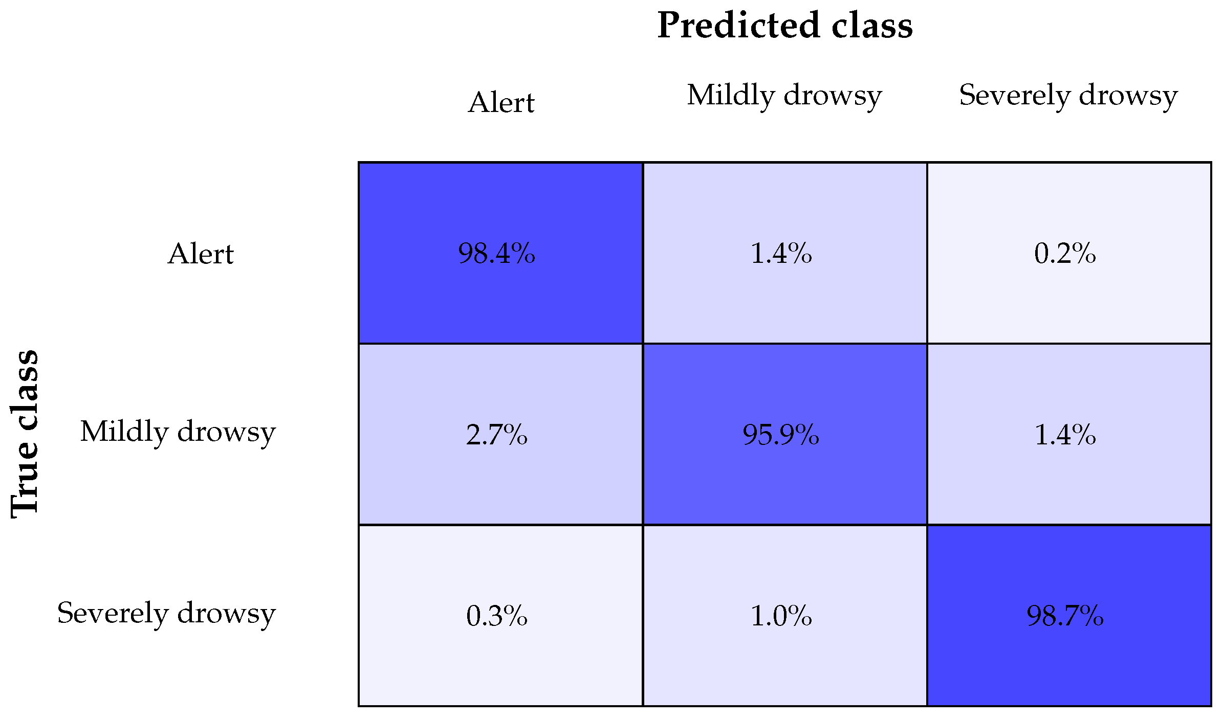
To transform these annotations into class labels suitable for supervised classification, a mapping is defined from KSS scores to a discrete set of fatigue levels. Let $k^{\left(s\right)}\left(t\right)$ denote the KSS score associated with subject s at time t. In the simplest case, $k^{\left(s\right)}\left(t\right)$ is constant within a session and equal to a session-level KSS score $k^{\left(s\right)}$. A label mapping function $g(·)$ is introduced so that $y^{\left(s\right)}\left(t\right)=g\left(k^{\left(s\right)}\left(t\right)\right)$, where $y^{\left(s\right)}\left(t\right)$ takes values in $\{1,\dots ,C\}$ and C denotes the number of fatigue classes. For example, in a three-class setting with alert, mildly drowsy, and severely drowsy states, the mapping can be defined as $g\left(k\right)=1$ if $1\le k\le 4$ for the alert class, $g\left(k\right)=2$ if $5\le k\le 6$ for the mildly drowsy class, and $g\left(k\right)=3$ if $7\le k\le 9$ for the severely drowsy class. When temporal windows ${\mathbf{X}}_n^{\left(s\right)}$ of length L are used as inputs, a single label $y_n^{\left(s\right)}$ is assigned to each window based on the KSS score associated with the time interval covered by that window. A simple choice is to use the session-level KSS score, in which case $y_n^{\left(s\right)}=g\left(k^{\left(s\right)}\right)$ for all windows extracted from that session. More refined strategies can also be adopted, for example aligning windows with time-varying KSS or reaction-time measurements when such information is available.

3.2.8. Construction of Training, Validation, and Test Sets

After pre-processing and labeling, the dataset can be expressed as a collection of labeled samples. In practice, we randomly assign $60\%$ of the subjects to ${\mathcal{S}}_{\mathrm{train}}$, $20\%$ to ${\mathcal{S}}_{\mathrm{val}}$, and the remaining $20\%$ to ${\mathcal{S}}_{\mathrm{test}}$.

To make the evaluation protocol fully explicit, the DROZY dataset was partitioned at the subject level before any model training or testing. Since the database contains 14 subjects in total, the nominal 60%/20%/20% split corresponds in practice to 8 subjects for training, 3 subjects for validation, and 3 subjects for testing. This yields an approximate subject ratio of 57.1%/21.4%/21.4%, which is the closest feasible integer split to the intended 60%/20%/20% partition.

Most importantly, all data from a given subject were assigned to a single subset only. Therefore, frames from the same subject never appear in more than one of the training, validation, and test sets. Because each subject in DROZY contributes multiple recording sessions, this also means that all sessions of the same subject remain within the same subset. As a result, no frame, sequence, or session from one subject can be shared across different partitions, which prevents identity leakage and ensures a strictly subject-independent evaluation protocol.

Table 3. Subject-level data partition used in the experiments.

Subset	No. of Subjects	Approx. Ratio	Session/Frame Sharing Across Subsets
Training	8	57.1%	No
Validation	3	21.4%	No
Test	3	21.4%	No

summarizes the final partition. This split ensures that the reported results reflect generalization to unseen subjects rather than memorization of subject-specific appearance or recording conditions.

3.3. TinyML Model Architecture

The proposed KAN-CLUE framework is organized as a compact convolutional–KAN architecture that is explicitly tailored for TinyML deployment on resource-constrained microcontrollers. The model comprises two main components. The first component is a very small convolutional neural network (CNN) that operates on the normalized eye or upper-face region and extracts a low-dimensional feature vector. The second component is a Kolmogorov–Arnold Network (KAN) head that receives this vector and produces uncertainty-aware fatigue predictions. The CNN is responsible for capturing local spatial patterns such as eyelid opening, blink-related texture, and periocular structure using a limited number of filters and pooling operations. The KAN head then provides flexible nonlinear transformations of these features with a parameter-efficient structure.

The input to the architecture is the normalized region of interest $X^{\left(s\right)}\left(t\right)\in {\mathbb{R}}^{H\times W}$ obtained from the pre-processing pipeline, where H and W denote the spatial resolution of the cropped eye or upper-face patch. For concreteness, and without loss of generality, we consider the case $H=W=48$ and a single input channel corresponding to the NIR intensity. The CNN feature extractor maps this $48\times 48\times 1$ tensor to a compact feature vector in ${\mathbb{R}}^{D_{\mathrm{emb}}}$, where $D_{\mathrm{emb}}$ is chosen to balance expressivity and TinyML feasibility. The KAN head then operates on this low-dimensional vector. In the following, the CNN feature extractor is described in detail, including its layer structure, mathematical formulation, parameter count, and approximate MAC complexity.

3.3.1. CNN Feature Extractor

The CNN feature extractor is a small two-layer network that maps each $48\times 48$ grayscale ROI to a compact embedding for the KAN head. It uses two $3\times 3$ convolutional layers with ReLU and $2\times 2$ max-pooling: the first layer has $C_1=8$ filters, the second has $C_2=16$ filters. After the two pooling operations, the feature maps are reduced to $12\times 12\times 16$ and flattened into a $D=2304$-dimensional vector, which is then projected by a fully connected layer to a $D_{\mathrm{emb}}=64$-dimensional embedding. In total, the CNN feature extractor has $P_{\mathrm{CNN}}=\mathrm{148,768}$ trainable parameters and requires $M_{\mathrm{CNN}}\approx 9.8\times {10}^5$ MACs per forward pass, which fits comfortably within typical TinyML memory and compute budgets when using 8-bit quantization.

3.3.2. Kan-Based Classification Head

The convolutional feature extractor described in the previous subsection produces, for each input region of interest, a compact embedding vector that summarizes the most salient periocular patterns related to driver fatigue. This embedding is denoted by ${\mathbf{z}}^{\mathrm{emb}}\in {\mathbb{R}}^{D_{\mathrm{emb}}}$, where $D_{\mathrm{emb}}$ is the embedding dimension, for example $D_{\mathrm{emb}}=64$ in the configuration considered here. In a conventional TinyML classifier, this vector would typically be fed into one or more fully connected layers with pointwise nonlinearities. In the KAN-CLUE framework, we replace this traditional dense head by one or two Kolmogorov–Arnold Network (KAN) layers that operate on ${\mathbf{z}}^{\mathrm{emb}}$ and produce a compact intermediate representation which is then mapped to class-wise evidence for fatigue prediction and uncertainty estimation.

A KAN layer approximates multivariate nonlinear mappings by composing learnable univariate functions along each input dimension with linear combinations across dimensions. Concretely, each KAN unit computes a weighted sum of univariate nonlinear transformations of the individual input coordinates. To make this idea compatible with TinyML constraints, each univariate function is parameterized using a low-order spline basis defined on a fixed grid, with a small number of basis functions and aggressively quantized control points.

The KAN head first normalizes the embedding coordinates to a common interval before applying spline-based univariate functions. Let ${\mathbf{z}}^{\mathrm{emb}}={[z_1,z_2,\dots ,z_{D_{\mathrm{emb}}}]}^{\top }$ denote the embedding, and let ${\mu }_r$ and ${\sigma }_r$ be precomputed mean and standard deviation values for dimension r. A normalized coordinate ${\tilde{z}}_r$ is defined as ${\tilde{z}}_r={\displaystyle \frac{z_r-{\mu }_r}{{\sigma }_r}}$, and then linearly rescaled and clipped to the unit interval $[0,1]$ by $u_r=\min \left(1,\max (0,a_r{\tilde{z}}_r+b_r)\right)$, where $a_r$ and $b_r$ are scalar parameters that define an affine transformation from the standardized space to the spline grid domain. In practice, $a_r$ and $b_r$ are chosen such that most values of ${\tilde{z}}_r$ lie in $[0,1]$ on the training set. This normalization step ensures that all univariate spline functions operate over the same fixed interval, which simplifies their implementation and facilitates sharing of precomputed basis functions across edges.

Each normalized coordinate $u_r$ is then passed through a univariate function ${\phi }_{i,r}(·)$ associated with hidden unit i and input dimension r. In KAN, these univariate functions are represented as linear combinations of basis functions defined on a fixed grid, typically B-splines or piecewise polynomial splines. In this work, we employ a uniform B-spline basis of low degree, for example linear or cubic, with a small number M of segments, which strikes a balance between approximation power and computational simplicity.

Let ${\left\{B_m(·)\right\}}_{m=1}^M$ denote a set of M basis functions supported on the unit interval $[0,1]$, for instance uniform B-splines of a chosen degree defined on a fixed knot vector. The univariate function ${\phi }_{i,r}$ is written as ${\phi }_{i,r}\left(u_r\right)={\sum }_{m=1}^M{\alpha }_{i,r,m}{B}_m\left(u_r\right)$, where ${\alpha }_{i,r,m}$ are learnable coefficients, or control points, associated with the M basis functions for the pair $(i,r)$. The set of all ${\alpha }_{i,r,m}$ determines the shape of the learned univariate function along dimension r for hidden unit i. In the most general case, each pair $(i,r)$ has its own collection of control points, but to improve efficiency on TinyML hardware, simplifications can be introduced, such as sharing control points across subsets of units or across all units corresponding to the same input dimension.

The output of the first KAN layer is obtained by linearly combining the univariate transformations ${\phi }_{i,r}\left(u_r\right)$ across input dimensions. Denoting the activation of hidden unit i by $h_i^{\left(1\right)}$, the KAN hidden layer is defined as $h_i^{\left(1\right)}=b_i^{\left(1\right)}+{\sum }_{r=1}^{D_{\mathrm{emb}}}{w}_{i,r}^{\left(1\right)}{\phi }_{i,r}\left(u_r\right)$, where $w_{i,r}^{\left(1\right)}$ is a scalar weight that modulates the contribution of the univariate function ${\phi }_{i,r}$ to unit i, and $b_i^{\left(1\right)}$ is a bias term. The index i runs from 1 to $H_{\mathrm{KAN}}$, where $H_{\mathrm{KAN}}$ denotes the number of hidden KAN units in the classification head. For TinyML deployment, $H_{\mathrm{KAN}}$ is chosen to be relatively small, for example $H_{\mathrm{KAN}}=32$, in order to limit the number of parameters and operations. An elementwise nonlinearity $\psi (·)$ may be applied to $h_i^{\left(1\right)}$, yielding the first-layer hidden representation $a_i^{\left(1\right)}=\psi \left(h_i^{\left(1\right)}\right)$, with $\psi (·)$ typically chosen as a smooth nonlinearity such as tanh or a rectified function. In practice, and especially under quantization constraints, using a simple and monotonic nonlinearity such as tanh or a clipped linear function helps to maintain numerical robustness.

If an additional KAN layer is employed, the activations ${\mathbf{a}}^{\left(1\right)}={[a_1^{\left(1\right)},\dots ,a_{H_{\mathrm{KAN}}}^{\left(1\right)}]}^{\top }$ serve as input to a second KAN layer of the same general form. For a second layer with $H_{\mathrm{KAN},2}$ units, one first defines normalized inputs $v_j$ obtained from $a_j^{\left(1\right)}$ through an affine transformation and clipping analogous to the unit-interval normalization described above, then parameterizes new univariate functions ${\tilde{\phi }}_{\mathcal{l},j}\left(v_j\right)$ as linear combinations of the same fixed basis $\left\{B_m(·)\right\}$, and combines them linearly as $h_{\mathcal{l}}^{\left(2\right)}=b_{\mathcal{l}}^{\left(2\right)}+{\sum }_{j=1}^{H_{\mathrm{KAN}}}{w}_{\mathcal{l},j}^{\left(2\right)}{\tilde{\phi }}_{\mathcal{l},j}\left(v_j\right)$, with corresponding activations $a_{\mathcal{l}}^{\left(2\right)}=\psi \left(h_{\mathcal{l}}^{\left(2\right)}\right)$. In many TinyML scenarios, a single KAN layer is already sufficiently expressive when combined with the CNN feature extractor, and thus the first-layer hidden representation alone is used. The optional second layer provides additional nonlinear capacity at the cost of extra parameters and MACs, and can be enabled or disabled depending on the available resources.

The final classification logits are produced by a linear layer that maps the KAN hidden representation to C output units, where C is the number of fatigue classes, for example $C=3$ corresponding to alert, mildly drowsy, and severely drowsy. If a single KAN layer is used, the logits are defined as $o_k=c_k+{\sum }_{i=1}^{H_{\mathrm{KAN}}}{v}_{k,i}{a}_i^{\left(1\right)}$ for $k\in \{1,\dots ,C\}$, where $v_{k,i}$ are the weights of the output layer and $c_k$ are the bias terms. When a second KAN layer is present, the same expression holds with $a_i^{\left(1\right)}$ replaced by $a_i^{\left(2\right)}$ and $H_{\mathrm{KAN}}$ replaced by $H_{\mathrm{KAN},2}$. The vector $\mathbf{o}={[o_1,\dots ,o_C]}^{\top }$ is then passed to the evidential output layer described elsewhere, which converts it into class-wise evidence and predictive uncertainty.

The KAN head has a relatively small number of trainable parameters compared to the CNN feature extractor. For a single KAN layer with $H_{\mathrm{KAN}}$ units, each applied to a $D_{\mathrm{emb}}$-dimensional embedding with M spline control points per input dimension, the total parameter count combines: (i) spline coefficients, (ii) linear mixing weights and biases in the hidden layer, and (iii) the output layer weights and biases. With the configuration used in this work, $D_{\mathrm{emb}}=64$, $H_{\mathrm{KAN}}=32$, $M=8$, and $C=3$ output classes, the KAN head contains $P_{\mathrm{KAN}-\mathrm{head}}=\mathrm{18,563}$ trainable parameters in total. This is substantially smaller than the $\mathrm{148,768}$ parameters of the CNN feature extractor and comfortably fits TinyML memory constraints once quantized.

From a computational standpoint, the dominant cost of a KAN layer lies in evaluating the spline expansions and performing the linear combinations in the hidden layer and output logits. If each basis function $B_m\left(u_r\right)$ is computed on the fly, evaluating ${\phi }_{i,r}\left(u_r\right)$ requires M multiplications and $(M-1)$ additions. However, in TinyML deployments, it is advantageous to precompute the basis function values on a fixed grid of L points in $[0,1]$ and store them in a look-up table. Each normalized input $u_r$ is then quantized to an index in this grid, and evaluating ${\phi }_{i,r}\left(u_r\right)$ reduces to fetching M basis values and performing M multiplications and additions with the quantized coefficients ${\alpha }_{i,r,m}$. As a result, the MAC complexity of the KAN layer scales approximately as $M_{\mathrm{KAN}-\mathrm{layer}}\approx H_{\mathrm{KAN}}·D_{\mathrm{emb}}·M+H_{\mathrm{KAN}}·D_{\mathrm{emb}}+C·H_{\mathrm{KAN}}$, where the first term accounts for the spline evaluations, the second term covers the linear combination weights $w_{i,r}^{\left(1\right)}$, and the third term corresponds to the output logits. Using the same example values as above, and ignoring the relatively small contribution of the output layer, the leading term is $H_{\mathrm{KAN}}·D_{\mathrm{emb}}·M=32·64·8=\mathrm{16,384}$, which is orders of magnitude smaller than the approximately ${10}^6$ MACs required by the CNN feature extractor. This confirms that the KAN head adds negligible computational overhead compared with the convolutional part of the model, while providing significantly enhanced flexibility and expressivity in the final classification stage.

To further adapt the KAN head to TinyML constraints, several simplifications are adopted. A single uniform spline grid is shared across all input dimensions and KAN units, so that the basis functions $B_m(·)$ and the knot vector are common and can be implemented once for all edges. Low-order splines, typically linear or at most cubic, are used to minimize the number of basis functions and avoid expensive higher-order polynomial evaluations. All control points ${\alpha }_{i,r,m}$, linear weights $w_{i,r}^{\left(1\right)}$ and $v_{k,i}$, and biases are quantized to 8-bit integers after training, and the normalized inputs $u_r$ are quantized to a fixed-point representation. This aggressive quantization, combined with shared grids and low-order splines, yields a KAN-based classification head that remains compatible with the constraints of microcontroller-class devices, yet preserves the key modeling advantage of KANs: the ability to learn rich, dimension-wise nonlinear transformations and combine them in a structured way for driver fatigue detection.

3.3.3. What Is Technically New in Kan-Clue?

KAN-CLUE is not intended as a claim that any one of its ingredients is individually unprecedented. Compact convolutional backbones, KAN layers, evidential uncertainty estimation, OOD scoring, and continual-learning regularization each exist in the literature in different forms. The novelty of the present work lies instead in how these components are specialized, coupled, and constrained for a single deployment target: uncertainty-aware continual driver fatigue detection on microcontroller-class TinyML hardware.

More specifically, the contribution goes beyond simply replacing a dense classifier with a KAN head. First, the KAN component is used as a compact evidential decision layer, not merely as a drop-in nonlinear classifier. The convolutional backbone produces a low-dimensional embedding, and the KAN head transforms this embedding into class-wise evidence that parameterizes a Dirichlet predictive distribution. This design lets the same lightweight head support both classification and predictive uncertainty estimation without requiring ensembles, Monte Carlo sampling, or a large Bayesian approximation.

Second, KAN-CLUE combines two complementary reliability signals within a TinyML-compatible pipeline: evidential uncertainty from the Dirichlet output and a lightweight activation-histogram OOD score computed from the embedded feature space. The role of the OOD module is not only to detect samples that deviate from the training distribution, but also to support decision gating and sample selection under severe edge constraints. This combination is particularly important for embedded fatigue monitoring, where false confidence on unusual facial appearances, lighting conditions, or driver-specific patterns can be operationally harmful.

Third, the continual-learning component is not a generic add-on. In KAN-CLUE, on-device adaptation is driven by the uncertainty/OOD logic and regularized through a KAN-aware consolidation mechanism. Rather than updating the entire model indiscriminately, the adaptation strategy selectively updates a small parameter subset and constrains it with an EWC-style penalty applied to the KAN-sensitive parameters, namely the spline/control-point representations and associated mixing weights that govern the nonlinear edge functions. This is different from a standard continual-learning treatment of dense layers, because the parameters being preserved and updated have a different structural role in KANs.

Finally, the overall contribution is architectural at the system level. The proposed framework is designed so that compact feature extraction, uncertainty-aware prediction, OOD detection, and controlled continual adaptation are all achieved within a single TinyML-ready pipeline. In this sense, the novelty is not the isolated existence of CNNs, KANs, evidential learning, OOD scoring, or continual learning, but the fact that they are integrated in a deployment-constrained and mutually reinforcing way for trustworthy driver fatigue detection at the IoT edge (see

Table 4. Component-wise positioning of the proposed framework. The table clarifies how each design element contributes beyond a standard compact CNN classifier.

Component	Role in KAN-CLUE
Compact CNN backbone	Extracts a low-dimensional visual embedding from NIR periocular inputs under strict TinyML memory and MAC constraints.
KAN head	Replaces a conventional dense head with structured learnable univariate transformations, increasing expressive power at low parameter cost.
Evidential formulation	Converts KAN outputs into class-wise evidence and Dirichlet uncertainty, enabling confidence-aware prediction without sampling or ensembles.
Activation-histogram OOD score	Provides a lightweight distribution-shift signal in the embedded feature space, suitable for MCU-class deployment.
Uncertainty/OOD-driven update policy	Uses reliability signals to decide when adaptation is needed, rather than updating continuously or indiscriminately.
KAN-aware continual regularization	Applies consolidation to the KAN-sensitive parameters that govern the learned edge functions, reducing forgetting during on-device adaptation.

).

3.3.4. Quantization and Deployment

The KAN-CLUE model is ultimately intended to run on microcontroller-class devices under the TinyML paradigm, where both compute and memory resources are highly constrained. In this context, quantization is a crucial step that converts the floating-point model trained on a workstation into an integer-arithmetic implementation suitable for deployment. The goal of this process is to reduce model size, improve inference speed, and lower energy consumption, while preserving as much predictive accuracy and calibration quality as possible.

After the CNN feature extractor and the KAN-based classification head have been trained in floating-point, typically using 32-bit single precision, a post-training quantization procedure is applied [33]. In post-training quantization, the learned weights and, optionally, the activations are converted from floating-point values to low-bit integer representations without modifying the training procedure itself. Let w denote a scalar weight in the floating-point model. The quantized version $\widehat{w}$ in an $b_w$-bit integer format, for example $b_w=8$, is obtained by applying an affine mapping parameterized by a scale factor $s_w$ and a zero-point $z_w$, followed by rounding and clipping to the representable integer range. This mapping can be written as $\widehat{w}={\mathrm{clip}}_{\mathcal{I}}\left(\mathrm{round}\left({\displaystyle \frac{w}{s_w}}\right)+z_w\right)$, where $\mathcal{I}$ denotes the set of integers representable in the chosen format, for example $\mathcal{I}=\{-128,\dots ,127\}$ for signed 8-bit quantization, and ${\mathrm{clip}}_{\mathcal{I}}(·)$ projects the value onto $\mathcal{I}$ if it falls outside this range. The corresponding dequantized value used in integer–float mixed analysis is given by $w\approx s_w\left(\widehat{w}-z_w\right)$, which is used internally to reason about the effect of quantization, even though at inference time the microcontroller operates directly on the integer representation $\widehat{w}$.

The same principle is applied to activations. Given a floating-point activation a at some layer, the quantized activation $\widehat{a}$ is $\widehat{a}={\mathrm{clip}}_{\mathcal{I}}\left(\mathrm{round}\left({\displaystyle \frac{a}{s_a}}\right)+z_a\right)$, where $s_a$ and $z_a$ are layer-specific scale and zero-point parameters obtained from calibration data or from the training distribution. The forward pass of the quantized model therefore consists primarily of integer MAC operations and integer additions, which can be implemented very efficiently on microcontrollers with support for SIMD-like instructions, for example ARM Cortex-M devices with DSP extensions.

In the context of KAN-CLUE, both the CNN parameters, namely convolutional kernels, biases, and fully connected weights, and the KAN-specific parameters, namely spline control points, linear combination weights, and biases, are quantized to 8-bit integers. The total number of trainable parameters in the CNN feature extractor was previously denoted by $P_{\mathrm{CNN}}$, and the number of parameters in the KAN head by $P_{\mathrm{KAN}-\mathrm{head}}$. The total parameter count of the complete model is $P_{\mathrm{tot}}=P_{\mathrm{CNN}}+P_{\mathrm{KAN}-\mathrm{head}}$. When using $b_w$ bits per parameter, the storage required to hold all weights and biases in non-volatile memory, for example Flash, can be approximated by $S_{\mathrm{Flash}}\approx P_{\mathrm{tot}}·{\displaystyle \frac{b_w}{8}}$ bytes. For instance, using the example values $P_{\mathrm{CNN}}=\mathrm{148,768}$ and $P_{\mathrm{KAN}-\mathrm{head}}=\mathrm{18,563}$ leads to $P_{\mathrm{tot}}=\mathrm{148,768}+\mathrm{18,563}=\mathrm{167,331}$, and with $b_w=8$ bits per parameter, one obtains $S_{\mathrm{Flash}}\approx \mathrm{167,331}·{\displaystyle \frac{8}{8}}=\mathrm{167,331}\mathrm{bytes}\approx 163.4$ kB, which comfortably fits within the Flash memory budgets of common TinyML platforms.

The memory required for intermediate activations during inference is stored in volatile memory, SRAM, and depends on the largest feature map that needs to be kept in memory at any point in the forward pass. An approximate bound on the activation memory can be obtained by summing the sizes of the main tensors that must coexist, multiplied by the number of bytes per activation. For 8-bit activations, the memory needed for a tensor with $N_{\mathrm{act}}$ elements is $S_{\mathrm{act}}\approx N_{\mathrm{act}}$ bytes. If the largest feature map in the CNN occurs after the first convolution, with dimensions $48\times 48\times 8$, then $N_{\mathrm{act},\max }=48·48·8=\mathrm{18,432}$, corresponding to approximately 18 kB of activation memory for that particular tensor. In practice, the memory allocator of the deployment framework, for example TensorFlow Lite Micro, reuses activation buffers across layers, and additional space is reserved for other tensors such as input, output, and auxiliary scratch buffers. The total RAM footprint is therefore slightly larger than the simple sum of tensor sizes, but remains within a typical budget of a few tens of kilobytes for the architectures considered here.

The KAN-specific operations are implemented in an efficient integer-friendly manner. During training, spline basis functions $B_m\left(u\right)$ are defined over the continuous interval $[0,1]$. For deployment, the interval is discretized into a regular grid of L points $u_j={\displaystyle \frac{j}{L-1}}$, with $j=0,1,\dots ,L-1$, and the basis functions are precomputed at these locations, yielding a look-up table of size $M\times L$, where M is the number of basis functions. The resulting table entries can themselves be quantized to a fixed-point representation with $b_B$ bits. The memory required to store this look-up table in Flash is approximately $S_{\mathrm{LUT}}\approx M·L·{\displaystyle \frac{b_B}{8}}$ bytes. For example, with $M=8$ basis functions, $L=64$ grid points, and $b_B=8$ bits, one obtains $S_{\mathrm{LUT}}\approx 8·64·{\displaystyle \frac{8}{8}}=512$ bytes, which is negligible compared with the overall model size.

At inference time, each normalized and quantized input $u_r$ is mapped to the closest grid points on this grid. Let $\Delta =1/(L-1)$ denote the grid spacing, and suppose that $u_r$ lies between $u_j$ and $u_{j+1}$. An index j is obtained as $j=⌊{\displaystyle \frac{u_r}{\Delta }}⌋$, and a local interpolation coefficient $\lambda \in [0,1]$ is computed as $\lambda ={\displaystyle \frac{u_r-u_j}{\Delta }}$. The value of a basis function $B_m\left(u_r\right)$ can then be approximated by linear interpolation between its precomputed values at $u_j$ and $u_{j+1}$, namely $B_m\left(u_r\right)\approx (1-\lambda )B_m\left(u_j\right)+\lambda B_m\left(u_{j+1}\right)$, where $B_m\left(u_j\right)$ and $B_m\left(u_{j+1}\right)$ are fetched from the look-up table. Since all quantities involved are represented in fixed-point, the interpolation step reduces to a small number of integer MACs and shifts, which are highly efficient on microcontrollers. The univariate spline ${\phi }_{i,r}\left(u_r\right)$ is then evaluated by combining these approximate basis values with quantized control points ${\alpha }_{i,r,m}$, resulting in a computation dominated by integer MACs and table look-up operations.

The entire quantized KAN-CLUE model is deployed using a lightweight inference framework such as TensorFlow Lite Micro or an equivalent embedded inference runtime. These frameworks provide a static memory arena for tensors, avoid dynamic memory allocation at runtime, and implement integer kernels for convolution, fully connected layers, activation functions, and generic elementwise operations. Custom kernels are implemented for the KAN-specific spline evaluation and interpolation routines, making use of the precomputed look-up tables and quantized control points. The compiled binary is generated with compiler optimizations enabled, for example -O3, and, where available, DSP-like instructions, such as ARM CMSIS-NN intrinsics, are used to accelerate integer MACs.

For clarity and completeness, the overall architecture can be summarized in a table that reports, for each major layer, the output tensor size, the number of trainable parameters, and the number of MACs. An example of such a summary is given in

Table 5. Architecture summary of the CNN + KAN-CLUE model for a $48\times 48$ single-channel input. The table reports, for each main layer, the output tensor size, the number of trainable parameters, and the approximate number of multiply–accumulate operations (MACs) per inference.

Layer	Output Size	Parameters	MACs
Input	$48\times 48\times 1$	−	−
${\mathrm{Conv}}_1$ (3 × 3, 8 ch)	$48\times 48\times 8$	$P_{{\mathrm{Conv}}_1}=80$	$M_{{\mathrm{Conv}}_1}=\mathrm{165,888}$
${\mathrm{MaxPool}}_1$ (2 × 2)	$24\times 24\times 8$	0	negligible
${\mathrm{Conv}}_2$ (3 × 3, 16 ch)	$24\times 24\times 16$	$P_{{\mathrm{Conv}}_2}=1168$	$M_{{\mathrm{Conv}}_2}=\mathrm{663,552}$
${\mathrm{MaxPool}}_2$ (2 × 2)	$12\times 12\times 16$	0	negligible
Flatten	$2304$	0	0
${\mathrm{Dense}}_1$ (to $D_{\mathrm{emb}}=64$)	64	$P_{\mathrm{FC}}=\mathrm{147,520}$	$M_{\mathrm{FC}}=\mathrm{147,456}$
KAN head (single layer)	$H_{\mathrm{KAN}}$	$P_{\mathrm{KAN}-\mathrm{head}}\approx \mathrm{18,563}$	$M_{\mathrm{KAN}-\mathrm{layer}}\approx \mathrm{16,384}$
Output (logits for $C=3$)	3	included in KAN head	included in KAN head
Total	−	$P_{\mathrm{tot}}\approx \mathrm{167,331}$	$M_{\mathrm{tot}}\approx 9.8\times {10}^5$

, which assumes the configuration described in the previous subsections.

3.4. Uncertainty Quantification with Evidential KAN

In conventional neural classifiers, the final layer typically produces real-valued logits, which are then passed through a softmax function to obtain class probabilities. While this yields point estimates, it does not explicitly represent the model’s confidence or epistemic uncertainty, and it is well known that softmax scores can be overconfident even on ambiguous or out-of-distribution inputs. In the context of safety-critical applications such as driver fatigue detection, this limitation is problematic, since a monitoring system should be able to recognize when its predictions are unreliable and react accordingly. To address this issue within the KAN-CLUE framework, we adopt an evidential learning formulation in which the output layer of the KAN head parameterizes a Dirichlet distribution over class probabilities. This evidential output layer provides, for each input, both an expected class probability vector and an associated measure of uncertainty that can be computed with negligible overhead on TinyML hardware.

3.4.1. Evidential Output Layer

Let the KAN head, possibly after one or two KAN layers as described previously, produce a vector of real-valued logits for a given input sample. Denote this vector by

$$\mathbf{z}={[z_1,z_2,\dots ,z_K]}^{\top },$$

(1)

where K is the number of classes, for example $K=3$ for alert, mildly drowsy, and severely drowsy states. In a standard classifier, these logits would be transformed directly into probabilities via a softmax. In the evidential setting, they are instead interpreted as parameters controlling the amount of evidence in favor of each class.

To ensure that the evidence values are non-negative and to maintain differentiability, a softplus function is applied to each logit. The softplus function is defined as

$$\mathrm{softplus}\left(x\right)=\log \left(1+e^x\right),$$

(2)

and behaves similarly to a smooth version of the ReLU activation. The evidence $e_k$ associated with class k is obtained by applying softplus to the corresponding logit $z_k$:

$$e_k=\mathrm{softplus}\left(z_k\right),k=1,\dots ,K.$$

(3)

By construction, $e_k\ge 0$ for all k, and larger values of $e_k$ correspond to stronger support for class k according to the model.

The evidence vector $\mathbf{e}={[e_1,\dots ,e_K]}^{\top }$ is then used to define the parameters of a Dirichlet distribution over the K-dimensional simplex of class probabilities. The Dirichlet distribution is parameterized by a vector of concentration parameters $\mathit{\alpha }={[{\alpha }_1,\dots ,{\alpha }_K]}^{\top }$, with ${\alpha }_k>0$ for all k. In the evidential formulation, these parameters are defined as

$${\alpha }_k=e_k+1,k=1,\dots ,K.$$

(4)

This choice ensures that in the absence of evidence ($e_k=0$ for all k), the Dirichlet distribution reduces to a uniform prior with ${\alpha }_k=1$, whereas as the evidence grows, the corresponding concentration parameters increase and the distribution becomes more peaked.

Given the Dirichlet parameters $\mathit{\alpha }$, the predictive class probabilities are defined as the mean of the Dirichlet distribution. The expected probability for class k is given by

$$p_k=\mathbb{E}[P_k\mid \mathit{\alpha }]={\displaystyle \frac{{\alpha }_k}{{\sum }_{j=1}^K{\alpha }_j}},k=1,\dots ,K,$$

(5)

where $P_k$ denotes the random variable representing the probability of class k. The denominator

$$S={\displaystyle \sum _{j=1}^K}{\alpha }_j$$

(6)

represents the total concentration or total evidence across all classes. The vector $\mathbf{p}={[p_1,\dots ,p_K]}^{\top }$ thus plays the role of the predicted class probability vector, but it is now accompanied by a notion of how strongly the model supports these probabilities.

A simple scalar measure of predictive uncertainty can be derived from the total concentration S. Intuitively, when S is large, the Dirichlet distribution is sharply concentrated around its mean, reflecting high confidence in the predicted probabilities. Conversely, when S is close to K (which corresponds to low or no evidence beyond the uniform prior), the Dirichlet is broad and the model is highly uncertain. A convenient uncertainty measure u can therefore be defined as

$$u={\displaystyle \frac{K}{S}}={\displaystyle \frac{K}{{\sum }_{j=1}^K{\alpha }_j}}.$$

(7)

By construction, u takes values in $(0,1]$, with u approaching 1 when ${\alpha }_k\approx 1$ for all classes (no evidence, high uncertainty), and u approaching 0 as the total evidence grows. In the KAN-CLUE framework, this scalar uncertainty score is used both to interpret the reliability of individual predictions and to drive downstream mechanisms such as uncertainty-aware continual learning and out-of-distribution detection.

From an implementation standpoint, the evidential output layer adds only a negligible overhead compared to a standard softmax-based classifier. The computation of $e_k$ in (3), ${\alpha }_k$ in (4), and $p_k$ in (5) involves a small number of exponentials, logarithms, additions, and divisions per class, which can be efficiently approximated or implemented in fixed-point arithmetic on microcontrollers. The uncertainty score in (7) is a simple rational function of the Dirichlet parameters and is therefore also computationally lightweight. Despite this low cost, the evidential formulation provides a principled probabilistic interpretation of the output of the KAN head, quantifying both the predicted class probabilities and the associated confidence in a way that is particularly well-suited for safety-critical TinyML applications such as driver fatigue detection.

3.4.2. Training Loss and Calibration

The evidential KAN output layer described in the previous subsection provides, for each input sample, a vector of Dirichlet concentration parameters $\mathit{\alpha }={[{\alpha }_1,\dots ,{\alpha }_K]}^{\top }$ and an associated mean probability vector $\mathbf{p}={[p_1,\dots ,p_K]}^{\top }$ given by

$$p_k={\displaystyle \frac{{\alpha }_k}{{\sum }_{j=1}^K{\alpha }_j}},k=1,\dots ,K.$$

(8)

To train the model in a supervised setting, we combine these outputs with the ground-truth class label. Let $\mathbf{y}={[y_1,\dots ,y_K]}^{\top }$ denote a one-hot encoding of the true class, where $y_c=1$ if c is the correct class and $y_k=0$ for $k\ne c$. A natural starting point is the cross-entropy between $\mathbf{y}$ and the predictive mean probabilities $\mathbf{p}$, defined as

$$\mathrm{CE}(\mathbf{y},\mathbf{p})=-{\displaystyle \sum _{k=1}^K}{y}_k\log p_k.$$

(9)

In the evidential framework, this cross-entropy can be interpreted as the negative log-likelihood under the expected categorical distribution induced by the Dirichlet, and it serves as the base loss that encourages the model to assign high Dirichlet mass to the correct class.

However, cross-entropy alone does not explicitly discourage the model from being overconfident on samples it cannot predict correctly. To address this, the evidential learning formulation introduces a regularization term that penalizes the allocation of large amounts of evidence in cases where the prediction is wrong, or where the data are ambiguous. The idea is that when the model cannot confidently discriminate between classes, it should prefer to output a diffuse Dirichlet distribution with low total concentration, rather than committing strongly to an incorrect class. One way to formalize this principle is to define a regularizer $\mathcal{R}$ that increases with the total evidence assigned to classes that are inconsistent with the target label.

A simple and effective regularizer can be constructed by measuring the squared difference between the target one-hot vector $\mathbf{y}$ and the normalized evidence-based probabilities $\mathbf{p}$, scaled by the total evidence. Let

$$S={\displaystyle \sum _{k=1}^K}{\alpha }_k$$

(10)

denote the total concentration parameter of the Dirichlet distribution. A regularizer of the form

$$\mathcal{R}(\mathbf{y},\mathit{\alpha })={\displaystyle \sum _{k=1}^K}{\left(y_k-p_k\right)}^{2}S$$

(11)

penalizes situations in which the predicted probabilities $\mathbf{p}$ deviate significantly from the true label $\mathbf{y}$ while the total evidence S is large. Intuitively, this encourages the network to either assign high evidence to the correct class (making $p_k$ close to $y_k$), or to keep S small when the prediction is uncertain. When the model is incorrect, the term ${(y_k-p_k)}^2$ is large for the ground-truth class, and the regularizer pushes the total evidence down, thereby increasing uncertainty instead of overconfidence.

The total training loss for a single sample can then be expressed as the sum of the base cross-entropy and the regularization term weighted by a hyperparameter $\lambda \ge 0$:

$$\mathcal{L}(\mathbf{y},\mathit{\alpha })=\mathrm{CE}(\mathbf{y},\mathbf{p})+\lambda \mathcal{R}(\mathbf{y},\mathit{\alpha }).$$

(12)

Over a training set with N samples indexed by n, the empirical loss used to optimize the network parameters is given by

$${\mathcal{L}}_{\mathrm{train}}={\displaystyle \frac{1}{N}}{\displaystyle \sum _{n=1}^N}\left[\mathrm{CE}\left({\mathbf{y}}^{\left(n\right)},{\mathbf{p}}^{\left(n\right)}\right)+\lambda \mathcal{R}\left({\mathbf{y}}^{\left(n\right)},{\mathit{\alpha }}^{\left(n\right)}\right)\right].$$

(13)

The first term in (13) drives the network to fit the class labels in the usual cross-entropy sense, while the second term modulates how much evidence the model is allowed to accumulate when it is wrong or uncertain. Larger values of $\lambda$ encourage the model to be more conservative, assigning lower evidence (and higher uncertainty) to ambiguous samples, whereas smaller values of $\lambda$ produce behavior closer to a standard overconfident classifier.

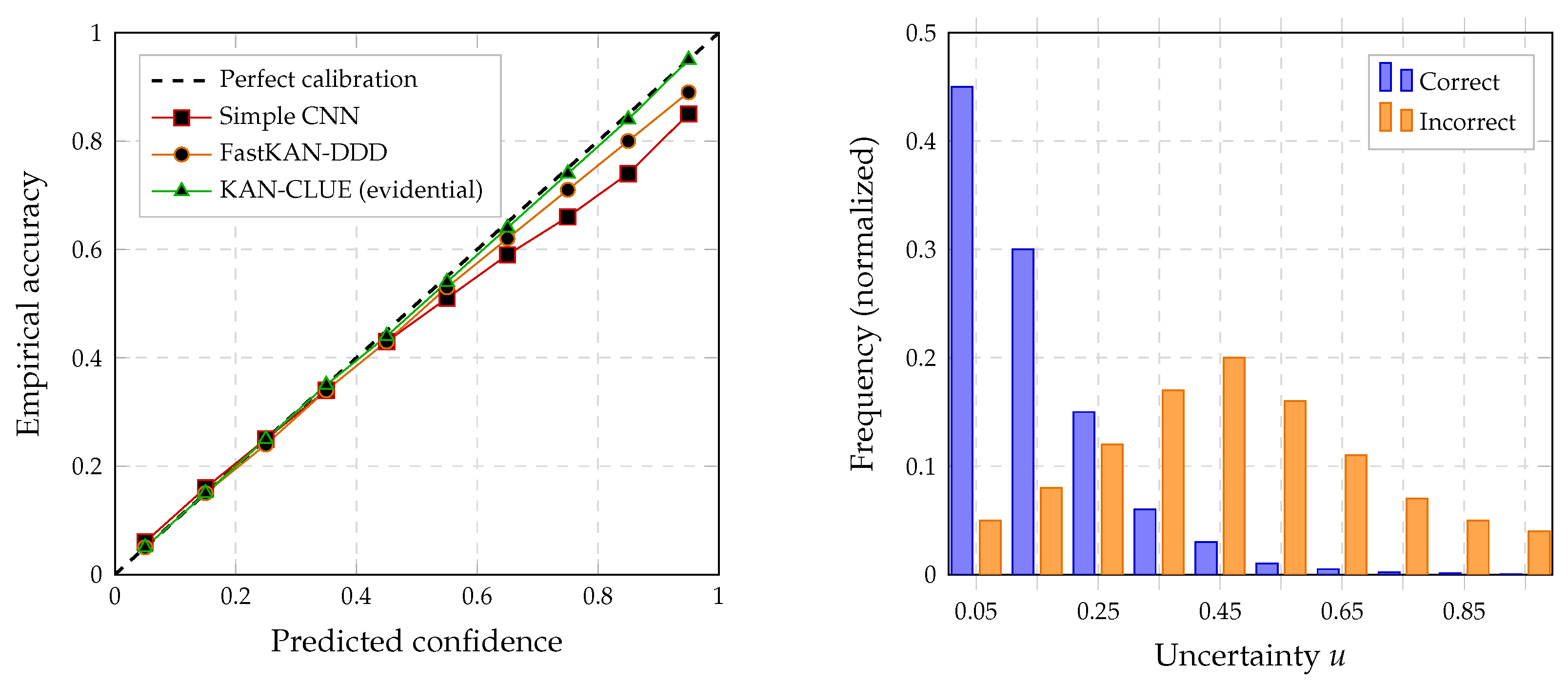
In practice, the choice of $\lambda$ and the calibration quality of the resulting model are assessed on a separate validation set. During training, different candidate values of $\lambda$ can be explored, either via a grid search or by gradually adjusting $\lambda$ based on calibration metrics measured on validation data. A common way to evaluate calibration is through reliability diagrams and the expected calibration error (ECE). Reliability diagrams plot, for a set of confidence bins, the empirical accuracy as a function of the mean predicted confidence within each bin. Well-calibrated models produce curves that lie close to the diagonal, indicating that predicted probabilities match empirical accuracies. Miscalibrated models, on the other hand, exhibit systematic deviations from this diagonal, which highlight overconfident or underconfident behavior.

The expected calibration error provides a scalar summary of the discrepancy between confidence and accuracy across all bins. Suppose the predictions on a validation set are partitioned into B disjoint confidence bins, and let $n_b$ denote the number of samples in bin b, $\mathrm{acc}\left(b\right)$ the empirical accuracy in that bin, and $\mathrm{conf}\left(b\right)$ the mean predicted confidence (for example ${\max }_k{p}_k$) in that bin. If $N_{\mathrm{val}}$ is the total number of validation samples, the ECE is defined as

$$\mathrm{ECE}={\displaystyle \sum _{b=1}^B}{\displaystyle \frac{n_b}{N_{\mathrm{val}}}}\left|\mathrm{acc}\left(b\right)-\mathrm{conf}\left(b\right)\right|.$$

(14)

Smaller values of $\mathrm{ECE}$ indicate better calibration. In the context of KAN-CLUE, the hyperparameter $\lambda$ in (12) can be tuned to minimize $\mathrm{ECE}$ on the validation set, subject to maintaining satisfactory classification performance. Additionally, thresholds on the uncertainty score u defined in (7) can be selected based on validation data to determine regimes of high, medium, and low confidence, which will later guide decision-making and continual learning mechanisms.

By combining the evidential loss in (13) with systematic calibration analysis via reliability diagrams and ECE, the KAN-CLUE framework produces predictions that are not only accurate but also accompanied by reliable measures of confidence. This is particularly important in driver fatigue detection, where overconfident errors can have serious consequences and where uncertainty-aware decisions provide a more trustworthy basis for in-vehicle assistance systems.

3.4.3. Using Uncertainty in Decision Logic

The evidential KAN output layer provides, for each input sample, both a predictive probability vector $\mathbf{p}={[p_1,\dots ,p_K]}^{\top }$ and an associated scalar uncertainty score u as defined in (7). In addition, the KAN activation-histogram mechanism yields an out-of-distribution score $S_{\mathrm{OOD}}$. Rather than relying solely on the most probable class for decision-making, the KAN-CLUE framework explicitly incorporates these uncertainty indicators into its decision logic. This is important in driver fatigue detection, where issuing overly assertive warnings in highly uncertain situations can lead to mistrust or nuisance alarms, whereas ignoring subtle but confident fatigue signals can compromise safety.

The most straightforward use of the evidential output is to identify the predicted class

$$\widehat{k}=\arg \underset{k\in \{1,\dots ,K\}}{\max }{p}_k,$$

(15)

and consider $\widehat{k}$ as the primary decision variable. However, the reliability of this decision is modulated by the uncertainty score u, which depends inversely on the total evidence accumulated by the Dirichlet distribution. To formalize this modulation, two thresholds are introduced on u, namely a lower threshold $u_{\mathrm{low}}$ and an upper threshold $u_{\mathrm{high}}$, with

$$0<u_{\mathrm{low}}<u_{\mathrm{high}}\le 1.$$

(16)

These thresholds partition the range of uncertainty values into three regimes that correspond to high-confidence, medium-confidence, and low-confidence predictions.

When the uncertainty score u is below the lower threshold $u_{\mathrm{low}}$, the model is considered to be highly confident in its prediction. Formally, the high-confidence regime is defined by

$$u<u_{\mathrm{low}}.$$

(17)

In this regime, the total evidence S in (6) is large, the Dirichlet distribution is sharply peaked around its mean, and the predicted class $\widehat{k}$ can be used directly to drive a strong and unambiguous decision, for example issuing a clear fatigue or non-fatigue alert according to the corresponding class of $\widehat{k}$. In practice, this regime is where the system behaves similarly to a traditional deterministic classifier, but with the additional reassurance that the internal uncertainty indicator supports such confidence.

When the uncertainty score u lies between $u_{\mathrm{low}}$ and $u_{\mathrm{high}}$, the prediction is considered to be of medium confidence. This intermediate regime is characterized by

$$u_{\mathrm{low}}\le u\le u_{\mathrm{high}}.$$

(18)

In this case, the model still provides a preferred class $\widehat{k}$, but the total evidence is moderate and the Dirichlet distribution is less concentrated. The system may still act on the predicted class, but in a softer manner. For example, if the predicted class corresponds to a fatigued state, the system may issue a preliminary or graded warning (such as a subtle visual indicator or a mild acoustic alert) instead of an aggressive intervention, and it may seek confirmation from additional observations over a short time window before escalating. This graded behavior reduces the risk of nuisance alarms while still leveraging useful information contained in medium-confidence predictions.

When the uncertainty score u exceeds the upper threshold $u_{\mathrm{high}}$, the prediction is deemed unreliable. The low-confidence regime is thus defined by

$$u>u_{\mathrm{high}}.$$

(19)

In this regime, the total evidence S is close to the baseline value K, indicating that the model has effectively not accumulated much evidence for any particular class, and the resulting Dirichlet distribution is broad. Acting aggressively on such predictions would be undesirable, as the model explicitly signals that it is unsure. Instead, the system can choose to suppress or down-weight the direct use of $\widehat{k}$ in the control loop, label the sample as “uncertain”, and possibly request additional information (for example, by integrating more frames or additional sensor data). If the OOD score $S_{\mathrm{OOD}}$ is also large for the same sample, this further strengthens the indication that the input lies outside the training distribution.

To incorporate OOD information, a threshold ${\tau }_{\mathrm{OOD}}$ is introduced on $S_{\mathrm{OOD}}$:

$$S_{\mathrm{OOD}}>{\tau }_{\mathrm{OOD}}$$

(20)

signals that the internal KAN activation patterns for the current sample are atypical compared with the training data. When either condition (19) or (20) is satisfied, the system marks the sample as unreliable. The corresponding decision rule can be summarized qualitatively as: if uncertainty is high or the OOD score is high, reduce the aggressiveness of any fatigue-related intervention, or flag the prediction as needing further evidence. In practice, this may translate into ignoring the immediate classification outcome or only logging the event without triggering an alert.

Samples that fall into the low-confidence or high-OOD regime are particularly valuable for continual learning. Their combination of uncertain prediction and atypical activations suggests that they may represent new conditions, such as a previously unseen driver, a novel illumination pattern, or a changed camera viewpoint. For this reason, KAN-CLUE stores such samples in a small replay buffer along with their predicted probabilities, uncertainty scores, OOD scores, and, when obtainable, corresponding labels or proxy labels. These buffered samples are then used during on-device adaptation phases to update a subset of KAN parameters in a regularized manner, as described in the continual learning section. In this way, the uncertainty-aware decision logic not only modulates real-time warnings but also guides the selection of informative data points for continual learning, allowing the TinyML model to evolve and specialize to new driving conditions while maintaining reliability and safety.

3.5. Uncertainty-Aware Continual Learning

The KAN-CLUE framework is designed not only to produce uncertainty-aware predictions, but also to adapt over time to changing driving conditions, new drivers, and evolving sensor characteristics. This adaptation is performed under strict TinyML constraints, which means that both the memory budget and the available computation for online updates are severely limited. To reconcile these constraints with the need for personalization and robustness, KAN-CLUE adopts an uncertainty-aware continual learning strategy in which only a small subset of carefully selected samples is stored on the device and later used to perform lightweight parameter updates. The selection of these samples is driven by the uncertainty and OOD scores described in Section 3.4, which helps focus the limited adaptation capacity on the most informative examples.

3.5.1. Online Data Collection

During deployment, the system processes an incoming stream of samples indexed by time $t=1,2,\dots$. For each new input frame (or temporal window) ${\mathbf{x}}_t$ that has been pre-processed into a normalized region of interest as described earlier, the KAN-CLUE model produces a predictive probability vector ${\mathbf{p}}_t={[p_{t,1},\dots ,p_{t,K}]}^{\top }$, an evidential uncertainty score $u_t$, and an OOD score $S_{\mathrm{OOD},t}$. The predicted class label ${\widehat{k}}_t$ is given by

$${\widehat{k}}_t=\arg \underset{k\in \{1,\dots ,K\}}{\max }{p}_{t,k},$$

(21)

and can be represented in one-hot form as a vector ${\widehat{\mathbf{y}}}_t$ with components

$${\widehat{y}}_{t,k}=\left\{\begin{array}{cc}1,\hfill & \mathrm{if}k={\widehat{k}}_t,\hfill \\ 0,\hfill & \mathrm{otherwise}.\hfill \end{array}\right.$$

(22)

The triplet $({\mathbf{p}}_t,u_t,S_{\mathrm{OOD},t})$, together with the raw input ${\mathbf{x}}_t$ or its embedded representation, forms the basic information associated with sample t.

To enable uncertainty-aware continual learning under memory constraints, KAN-CLUE maintains a fixed-size buffer that stores a limited number of recent or informative samples. Let B denote the maximum buffer capacity, for example $B\in [50,100]$, and let

$${\mathcal{B}}_t={\left\{({\tilde{\mathbf{x}}}_n,{\tilde{\mathbf{y}}}_n,u_n,S_{\mathrm{OOD},n})\right\}}_{n=1}^{|{\mathcal{B}}_t|}$$

(23)

represent the buffer contents at time t, where $|{\mathcal{B}}_t|\le B$ and ${\tilde{\mathbf{x}}}_n$ denotes either the raw normalized input, the compressed embedding ${\mathbf{z}}^{\mathrm{emb}}$, or a combination thereof. Storing the embedding instead of the raw frame can substantially reduce the memory footprint, as ${\mathbf{z}}^{\mathrm{emb}}\in {\mathbb{R}}^{D_{\mathrm{emb}}}$ is typically much smaller than the full image. In this case, the stored input representation is given by

$${\tilde{\mathbf{x}}}_t={\mathbf{z}}_t^{\mathrm{emb}},$$

(24)

The buffer is updated online as new samples arrive. At each time step t, the system decides whether to store the current sample $({\mathbf{x}}_t,{\mathbf{p}}_t,u_t,S_{\mathrm{OOD},t})$ in the buffer based on its uncertainty and OOD characteristics. The intuition is that samples with very low uncertainty and low OOD score are already well captured by the current model, whereas samples with extremely high uncertainty or OOD score may be too noisy or anomalous to be useful for stable adaptation. Therefore, KAN-CLUE focuses on samples in an intermediate regime of informativeness. A simple selection rule can be expressed using two constants $u_{\min }$ and $u_{\max }$, with $0<u_{\min }<u_{\max }\le 1$, and an OOD threshold ${\tau }_{\mathrm{OOD}}$. The sample at time t is considered for inclusion in the buffer if

$$u_{\min }\le u_t\le u_{\max }\mathrm{or}{S}_{\mathrm{OOD},t}>{\tau }_{\mathrm{OOD}},$$

(25)

that is, if it has moderate uncertainty or if it lies significantly outside the training distribution. When (25) holds and the buffer is not yet full, the sample is appended to ${\mathcal{B}}_t$. If the buffer is full, a replacement strategy is used, such as discarding the oldest entry (first-in first-out) or preferentially removing samples with low uncertainty that are less likely to drive useful updates.

The contents of the buffer must be associated with labels in order to perform supervised continual learning updates. In some scenarios, ground-truth labels for online samples may be available, for example through manual annotation or explicit driver feedback (such as a button indicating that the driver feels drowsy). Let $y_t$ denote the true class label for sample t, if available, and let ${\mathbf{y}}_t$ be its one-hot encoding. In this case, the stored label component ${\tilde{\mathbf{y}}}_t$ in (23) is set to the ground-truth one-hot vector:

$${\tilde{\mathbf{y}}}_t={\mathbf{y}}_t.$$

(26)

In many realistic deployments, however, explicit labels may not be available or may be provided only sporadically. Under such constraints, KAN-CLUE can operate with weak or proxy labels derived from heuristic rules, physiological signals, or aggregated model predictions.

One possible weak labeling strategy is to combine the model’s own predictions over short time windows with simple heuristics based on observable quantities such as eye closure duration or PERCLOS (percentage of eyelid closure). For example, if a sequence of frames exhibits prolonged eye closure or a high PERCLOS value, the corresponding samples can be weakly labeled as “fatigued” even in the absence of explicit ground truth. Formally, a weak label ${\tilde{\mathbf{y}}}_t$ is assigned based on a function $\mathcal{H}$ that maps observable features (including but not limited to the model output) to a one-hot vector:

$${\tilde{\mathbf{y}}}_t=\mathcal{H}\left({\mathbf{p}}_t,u_t,{\mathrm{PERCLOS}}_t,\dots \right),$$

(27)

where ${\mathrm{PERCLOS}}_t$ denotes a simple eye-closure metric at time t and the ellipsis represents other possible indicators such as blink rate or head pose cues. The function $\mathcal{H}$ can be implemented as a thresholding rule that associates high-eye-closure intervals with fatigued labels and low-eye-closure intervals with alert labels, leaving ambiguous cases unlabeled or labeled as “unknown” and not used for training.

Alternatively, in a self-supervised or unsupervised adaptation scenario where no labels or reliable proxies are available, KAN-CLUE can still exploit the stored samples to refine its internal representation without relying on explicit class labels. This can be achieved by using pseudo-labels derived from the model’s own high-confidence predictions, or by employing auxiliary consistency objectives that encourage stability of predictions under data augmentation or temporal perturbations. For pseudo-labeling, a sample is assigned a pseudo-label ${\tilde{\mathbf{y}}}_t$ equal to ${\widehat{\mathbf{y}}}_t$ from (22) only if its uncertainty $u_t$ is below a stricter threshold ${\tilde{u}}_{\mathrm{low}}$:

$${\tilde{\mathbf{y}}}_t=\left\{\begin{array}{cc}{\widehat{\mathbf{y}}}_t,\hfill & \mathrm{if}{u}_t<{\tilde{u}}_{\mathrm{low}},\hfill \\ \mathrm{undefined},\hfill & \mathrm{otherwise},\hfill \end{array}\right.$$

(28)

with undefined labels excluded from supervised updates. In this way, only highly confident predictions contribute to self-training, which mitigates the risk of reinforcing incorrect labels.

Regardless of the specific source of labels—true labels, weak labels, or pseudo-labels—the buffer ${\mathcal{B}}_t$ thus contains a small set of representative and informative samples $({\tilde{\mathbf{x}}}_n,{\tilde{\mathbf{y}}}_n,u_n,S_{\mathrm{OOD},n})$ that characterize the new operating regime encountered by the system. During idle periods or scheduled adaptation intervals, the KAN-CLUE framework uses these buffered samples to perform regularized updates of the KAN parameters on-device, as described in the subsequent subsections. This online data collection strategy is therefore a crucial link between uncertainty-aware prediction and resource-constrained continual learning in TinyML-based driver fatigue detection.

3.5.2. Sample Selection Using Uncertainty and OOD

The uncertainty and out-of-distribution scores produced by the evidential KAN head play a central role in deciding which samples should be stored in the replay buffer and subsequently used for continual learning. At each time step t, the model processes an input ${\mathbf{x}}_t$ and outputs the class-probability vector ${\mathbf{p}}_t={[p_{t,1},\dots ,p_{t,K}]}^{\top }$, the scalar uncertainty score $u_t$, and the OOD score $S_{\mathrm{OOD},t}$. The objective of the selection strategy is to focus limited memory and adaptation capacity on samples that are informative about the current distribution shift, while avoiding both uninformative and overly noisy examples.

Conceptually, samples with very low uncertainty are already well explained by the current model and lie in regions of the input space that the model has seen frequently during training. Including too many such samples in the buffer would lead to redundant updates that bring little new information. Conversely, samples with extremely high uncertainty or very large OOD scores may correspond to severe noise, sensor glitches, or extreme outliers, which can destabilize the learning process if used directly for parameter updates. Therefore, the selection mechanism targets an intermediate regime of uncertainty, while also giving special attention to samples that exhibit clear signs of distribution shift.

To formalize this, two uncertainty thresholds $u_{\min }$ and $u_{\max }$ are introduced, with

$$0<u_{\min }<u_{\max }\le 1,$$

(29)

and a threshold ${\tau }_{\mathrm{OOD}}$ is defined on the OOD score. A sample at time t is considered eligible for storage in the buffer when its uncertainty falls within the prescribed interval,

$$u_{\min }\le u_t\le u_{\max },$$

(30)

which captures moderately uncertain predictions that are likely to be informative rather than purely noisy. In addition, samples with an OOD score exceeding the threshold,

$$S_{\mathrm{OOD},t}>{\tau }_{\mathrm{OOD}},$$

(31)

are also marked as candidates for storage, since they signal a potential distribution shift even if their uncertainty is not in the moderate range. In practice, the selection rule at time t can be expressed as storing the sample whenever at least one of the conditions (30) or (31) is satisfied. When a candidate sample arrives and the buffer is full, a replacement policy is used that preferentially discards older or less informative samples, for instance by removing entries with low uncertainty or low OOD scores first.

Through (29)–(31), the model dynamically curates a compact set of samples that are most representative of the novel conditions encountered during deployment. These samples are therefore well suited to guide subsequent adaptation of the KAN parameters, while the avoidance of extremely low-uncertainty and extremely high-uncertainty examples helps maintain stability and efficiency in the continual learning process.

3.5.3. Parameter Update Scheme

Once the replay buffer has accumulated a small set of informative samples, the KAN-CLUE framework performs lightweight parameter updates in order to adapt to the new distribution while respecting TinyML constraints. Because memory and computation are limited, it is neither feasible nor desirable to update all parameters of the CNN and KAN head. Instead, only a restricted subset of parameters is adapted, and the updates are carried out intermittently, for example when the vehicle is stopped, when the driver is idle, or at low frequency during operation.

In the configuration considered here, the parameters chosen for adaptation are those of the final KAN-based classification stage, which directly maps the KAN hidden representation to class evidence. Let ${\mathit{\theta }}_{\mathrm{adapt}}$ denote the vector of parameters that are allowed to change online, and let ${\mathit{\theta }}_{\mathrm{base}}$ denote the original values of these parameters learned during offline training. A simple choice is to include in ${\mathit{\theta }}_{\mathrm{adapt}}$ the output layer weights and biases

$${\mathit{\theta }}_{\mathrm{adapt}}={\left\{v_{k,i},c_k\right\}}_{k=1,\dots ,K}^{i=1,\dots ,H_{\mathrm{KAN}}},$$

(32)

while keeping all CNN parameters and spline control points ${\alpha }_{i,r,m}$ fixed. This already provides a degree of adaptation by reweighting the KAN hidden units according to the new operating conditions. An alternative, slightly more flexible scheme is to introduce a small adapter layer on top of the KAN hidden representation. For instance, one can define an additional linear mapping

$${\mathbf{h}}^{\mathrm{adapt}}=W^{\mathrm{adapt}}{\mathbf{a}}^{\left(1\right)}+{\mathbf{b}}^{\mathrm{adapt}},$$

(33)

where ${\mathbf{a}}^{\left(1\right)}\in {\mathbb{R}}^{H_{\mathrm{KAN}}}$ denotes the first-layer KAN activations, $W^{\mathrm{adapt}}\in {\mathbb{R}}^{H_{\mathrm{adapt}}\times H_{\mathrm{KAN}}}$ and ${\mathbf{b}}^{\mathrm{adapt}}\in {\mathbb{R}}^{H_{\mathrm{adapt}}}$ are adapter parameters, and $H_{\mathrm{adapt}}$ is a small adapter dimension. The logits are then computed from ${\mathbf{h}}^{\mathrm{adapt}}$ rather than directly from ${\mathbf{a}}^{\left(1\right)}$, and only the adapter parameters $W^{\mathrm{adapt}}$ and ${\mathbf{b}}^{\mathrm{adapt}}$ are updated online. This isolates adaptation to a very small parameter subset and further reduces the risk of catastrophic forgetting.

Regardless of the exact choice of ${\mathit{\theta }}_{\mathrm{adapt}}$, the continual learning updates are performed using mini-batches drawn from the buffer. Let $\mathcal{B}$ denote the current buffer contents, and let ${\mathcal{B}}^{\mathrm{upd}}$ denote a mini-batch of size $B_{\mathrm{upd}}$ sampled from $\mathcal{B}$. For each sample in ${\mathcal{B}}^{\mathrm{upd}}$, the model computes the evidential KAN loss $\mathcal{L}({\tilde{\mathbf{y}}}_n,{\mathit{\alpha }}_n)$ as in (12), where ${\tilde{\mathbf{y}}}_n$ is the stored label (true, weak, or pseudo) and ${\mathit{\alpha }}_n$ are the current Dirichlet parameters produced by the adapted model. To prevent the adapted parameters from drifting too far from their original values and thereby degrading performance on previously seen conditions, a regularization term is added that penalizes large deviations from ${\mathit{\theta }}_{\mathrm{base}}$. A quadratic anchoring penalty of the form

$${\mathcal{R}}_{\mathrm{anchor}}={\displaystyle \frac{\gamma }{2}}{∥{\mathit{\theta }}_{\mathrm{adapt}}-{\mathit{\theta }}_{\mathrm{base}}∥}_2^2$$

(34)

is used, where $\gamma >0$ controls the strength of the constraint. The total loss for a mini-batch ${\mathcal{B}}^{\mathrm{upd}}$ is then given by

$${\mathcal{L}}_{\mathrm{CL}}={\displaystyle \frac{1}{B_{\mathrm{upd}}}}\sum _{({\tilde{\mathbf{x}}}_n,{\tilde{\mathbf{y}}}_n)\in {\mathcal{B}}^{\mathrm{upd}}}\mathcal{L}\left({\tilde{\mathbf{y}}}_n,{\mathit{\alpha }}_n\right)+{\mathcal{R}}_{\mathrm{anchor}},$$

(35)

where $\mathcal{L}(·,·)$ is the per-sample evidential loss from (12) and ${\mathit{\alpha }}_n$ are computed with the current values of ${\mathit{\theta }}_{\mathrm{adapt}}$.

The parameters ${\mathit{\theta }}_{\mathrm{adapt}}$ are updated by stochastic gradient descent or a related optimizer with a small learning rate ${\eta }_{\mathrm{CL}}$. A generic gradient descent update at adaptation step $\tau$ can be written as

$${\mathit{\theta }}_{\mathrm{adapt}}^{(\tau +1)}={\mathit{\theta }}_{\mathrm{adapt}}^{\left(\tau \right)}-{\eta }_{\mathrm{CL}}{\nabla }_{{\mathit{\theta }}_{\mathrm{adapt}}}{\mathcal{L}}_{\mathrm{CL}}^{\left(\tau \right)},$$

(36)

where ${\mathcal{L}}_{\mathrm{CL}}^{\left(\tau \right)}$ denotes the loss evaluated on the current mini-batch at step $\tau$. The number of adaptation steps $T_{\mathrm{CL}}$ performed in one adaptation phase is kept small, for example on the order of a few tens of gradient steps, in order to limit computation and energy consumption.

From an operational perspective, these continual learning updates are scheduled so as not to interfere with real-time monitoring. One simple strategy is to trigger adaptation only when the vehicle is stationary, for example when the speed is zero or below a small threshold, or when the ignition is turned on or off and the microcontroller has some spare time before shutdown. Another strategy is to perform updates periodically at a low frequency, such as once every few minutes, while ensuring that the total number of gradient steps per unit time remains within the device’s energy budget. In both cases, the use of a small buffer, a restricted parameter subset, and a regularized loss in (35) allows KAN-CLUE to gradually personalize its behavior to new drivers and conditions, without compromising its TinyML deployment constraints or its baseline performance on previously seen scenarios.

3.5.4. Regularization Against Catastrophic Forgetting (KAN-EWC-like)

While uncertainty-aware sample selection and restricted parameter updates already mitigate catastrophic forgetting, online adaptation can still degrade performance on previously learned conditions if the updated KAN parameters drift too far from their original values. To counter this effect in a more principled way, KAN-CLUE incorporates a regularization mechanism inspired by Elastic Weight Consolidation (EWC), tailored specifically to the structure of KAN. The central idea is to assign an importance score to each KAN parameter, with particular emphasis on the spline control points that define the univariate functions, and to penalize changes to parameters in proportion to their importance. Parameters that are critical for the original task are thus constrained to remain close to their offline values, while less important parameters are free to adapt more.

In the KAN head, each univariate spline function is parameterized by a set of control points. If the KAN layer has $H_{\mathrm{KAN}}$ hidden units and receives $D_{\mathrm{emb}}$ input dimensions, and each univariate function uses M spline basis functions, then the control points can be indexed by a single index e that runs over all edge–basis combinations. Formally, each parameter ${\varphi }_e$ corresponds to a particular control point ${\alpha }_{i,r,m}$, and the index set $\mathcal{E}$ collects all such edges:

$$\mathcal{E}=\left\{e\equiv (i,r,m)|i=1,\dots ,H_{\mathrm{KAN}},r=1,\dots ,D_{\mathrm{emb}},m=1,\dots ,M\right\}.$$

(37)

For each $e\in \mathcal{E}$, the parameter value at the end of offline training is denoted by ${\varphi }_e^{\left(0\right)}$. These offline values constitute the “reference” KAN configuration that should be preserved as much as possible while still allowing useful adaptation. The corresponding adapted value during online learning is denoted by ${\varphi }_e$, and the deviation ${\varphi }_e-{\varphi }_e^{\left(0\right)}$ measures how far the parameter has moved from its original setting.

To quantify the importance of each parameter ${\varphi }_e$, an importance score ${\Omega }_e$ is computed offline using the original training data. Intuitively, parameters that have a strong influence on the training loss for the original task should receive higher importance and be penalized more strongly during online updates. One practical way to define ${\Omega }_e$ is to use a gradient-based approximation, reminiscent of the diagonal of the Fisher information matrix in EWC. Let ${\mathcal{D}}_{\mathrm{offline}}$ denote the original training dataset and ${\mathcal{L}}_{\mathrm{offline}}$ the offline training loss (for example the evidential loss in (13)). For a given sample $(\mathbf{x},\mathbf{y})$ from ${\mathcal{D}}_{\mathrm{offline}}$, the gradient of the loss with respect to ${\varphi }_e$ is

$$g_e(\mathbf{x},\mathbf{y})={\displaystyle \frac{\partial }{\partial {\varphi }_e}}{\mathcal{L}}_{\mathrm{offline}}(\mathbf{y},\mathit{\alpha }\left(\mathbf{x}\right)),$$

(38)

where $\mathit{\alpha }\left(\mathbf{x}\right)$ denotes the Dirichlet parameters produced by the KAN head for input $\mathbf{x}$ under the offline-trained model. The importance score ${\Omega }_e$ is then defined as the average squared gradient over the training set:

$${\Omega }_e={\displaystyle \frac{1}{|{\mathcal{D}}_{\mathrm{offline}}|}}\sum _{(\mathbf{x},\mathbf{y})\in {\mathcal{D}}_{\mathrm{offline}}}{\left(g_e(\mathbf{x},\mathbf{y})\right)}^2.$$

(39)

This quantity approximates the sensitivity of the offline loss to changes in ${\varphi }_e$: if small perturbations in ${\varphi }_e$ cause large changes in the loss, then ${\Omega }_e$ will be large, indicating that ${\varphi }_e$ is important and should be preserved during online adaptation. Conversely, parameters with small ${\Omega }_e$ can be modified more freely without significantly affecting the original performance.

The importance scores ${\Omega }_e$ and the reference parameters ${\varphi }_e^{\left(0\right)}$ are computed once after offline training and stored in non-volatile memory. Because only the KAN control points (and optionally a small subset of additional KAN parameters) are considered, the total number of importance scores remains manageable for TinyML deployment. During online learning, these scores are used to construct an EWC-like regularization term that penalizes deviations of the adapted parameters from their reference values in proportion to their importance.

Let ${\mathcal{L}}_{\mathrm{current}}$ denote the loss used for online adaptation on buffered samples, such as ${\mathcal{L}}_{\mathrm{CL}}$ in (35) without the anchoring term. The KAN-EWC-like regularized online loss is then defined as

$${\mathcal{L}}_{\mathrm{online}}={\mathcal{L}}_{\mathrm{current}}+\lambda \sum _{e\in \mathcal{E}}{\Omega }_e{\left({\varphi }_e-{\varphi }_e^{\left(0\right)}\right)}^2,$$

(40)

where $\lambda \ge 0$ is a hyperparameter that controls the overall strength of the regularization. The second term in (40) acts as a quadratic penalty that grows rapidly when a highly important parameter ${\varphi }_e$ deviates from its original value ${\varphi }_e^{\left(0\right)}$. Parameters with small ${\Omega }_e$ are effectively less constrained and can be adapted more freely to fit the new data in the replay buffer.

The gradient of the regularized loss with respect to ${\varphi }_e$ is given by

$${\displaystyle \frac{\partial {\mathcal{L}}_{\mathrm{online}}}{\partial {\varphi }_e}}={\displaystyle \frac{\partial {\mathcal{L}}_{\mathrm{current}}}{\partial {\varphi }_e}}+2\lambda {\Omega }_e\left({\varphi }_e-{\varphi }_e^{\left(0\right)}\right),$$

(41)

which can be seamlessly integrated into the gradient descent update rule in (36). The additional term in (41) pulls each parameter ${\varphi }_e$ back toward ${\varphi }_e^{\left(0\right)}$ with a strength proportional to its importance score ${\Omega }_e$ and the chosen $\lambda$. This mechanism effectively creates a “soft constraint” that preserves the functionality learned during offline training, particularly for parts of the KAN head that are crucial for the original task.

From an implementation perspective, the EWC-like regularization requires storing only two additional quantities for each KAN control point: the reference value ${\varphi }_e^{\left(0\right)}$ and the importance score ${\Omega }_e$. Both can be quantized to low-bit fixed-point representations to conform with TinyML memory constraints. Because the EWC penalty in (40) is quadratic and separable across parameters, its computation during online updates involves only a small number of additional integer multiplications and additions per parameter, which adds negligible computational overhead relative to the main forward and backward passes.

By focusing the EWC-like regularization on the KAN spline control points, which encode the shape of the univariate nonlinearities, KAN-CLUE preserves the core structure of the learned representation while still allowing the output weights or small adapter layers to adjust to new conditions. This KAN-EWC-like mechanism thus provides a principled and efficient way to regularize online adaptation against catastrophic forgetting, ensuring that continual learning enhances performance in new regimes without sacrificing the reliability achieved during offline training on the DROZY dataset.

4. Experimental Setup

4.1. Embedded Hardware and Software

The proposed KAN-CLUE framework is designed with explicit TinyML constraints in mind and is therefore evaluated on a representative microcontroller-class platform rather than on desktop hardware only. In our experiments, we target a 32-bit ARM Cortex-M–class microcontroller with single-precision floating-point support and DSP extensions, running at a clock frequency in the range of 80–200 MHz. A typical configuration includes on the order of RAM ≈ 256 kB and Flash ≈ 1 MB, which is sufficient to store the quantized KAN-CLUE model weights, the TensorFlow Lite Micro (TFLM) runtime [34], and the intermediate activations needed for inference. As described in Section 3.3, the total number of model parameters $P_{\mathrm{tot}}$ translates into a Flash footprint of roughly $S_{\mathrm{Flash}}\approx P_{\mathrm{tot}}·{\displaystyle \frac{8}{8}}$ bytes, when using 8-bit quantization, leading to a model size on the order of a few hundred kilobytes, which comfortably fits within the Flash memory of the selected MCU.

On the software side, the entire model is deployed using a lightweight inference framework based on TFLM, augmented with custom integer kernels for the KAN-specific spline evaluation and histogram-based OOD scoring. The TFLM runtime provides a static memory arena for tensors and avoids dynamic memory allocation during inference, which is critical in the microcontroller environment. Convolutional and dense layers are implemented using optimized integer kernels, for example leveraging vendor-specific DSP libraries or CMSIS-NN intrinsics. The compiler toolchain is configured with full optimization enabled, typically using an option such as -O3, along with flags that enable hardware floating-point or DSP units when available. To improve fixed-point performance, fast-math and fused-multiply–add options may be enabled, and the KAN kernels are implemented in a way that minimizes branching and relies on precomputed look-up tables for spline basis values and logarithms. Latency is measured directly on the target microcontroller by toggling a GPIO pin around the inference call and recording the corresponding duration in milliseconds, while memory usage is inferred from the static allocation report produced by the TFLM memory planner.

To make the deployment study fully reproducible, we report here the exact embedded configuration used for inference, the quantization setting, the scope of the latency measurements, the power-measurement methodology, and the execution regime adopted for continual learning. The on-device evaluation targets the quantized inference stage of KAN-CLUE on a microcontroller-class platform, whereas model adaptation experiments are used to evaluate the continual-learning mechanism under controlled conditions.

Table 6. Deployment configuration and execution scope used for the embedded evaluation of KAN-CLUE.

Item	Configuration
Target MCU/board	STM32F427VIT6-based ARM Cortex-M4 platform
Clock frequency	168 MHz
On-chip Flash/SRAM	2 MB Flash/256 kB SRAM
Inference runtime	TensorFlow Lite for Microcontrollers (TFLM) with static tensor arena
Deployment model format	Fully quantized INT8 TFLite Micro model exported as a C array
Weight quantization	Signed INT8, per-channel symmetric quantization
Activation quantization	INT8, per-tensor asymmetric quantization
Bias/accumulation precision	INT32
Calibration procedure	Representative calibration subset drawn from the training split
Input tensor at deployment	One preprocessed NIR ROI of size $48\times 48\times 1$
Warm-up runs	100
Measured runs	1000 repeated inferences
Latency scope	Quantized model inference only
Included in latency	TFLM invocation, tensor loading, KAN head, evidential output, OOD scoring
Excluded from latency	ROI extraction, landmarking, resizing, normalization, and host-side data transfer
Power measurement methodology	Real hardware measurement on the target board using an inline shunt-based current-monitoring setup under a regulated $3.3$ V supply; average active power computed over the same 1000-run inference protocol
Continual learning execution	Simulated offline on workstation; not executed on the MCU

summarizes the exact deployment protocol. The reported MCU latency corresponds to the execution of the quantized KAN-CLUE model on an already prepared $48\times 48\times 1$ NIR region-of-interest tensor. In other words, the timing measurements begin once the ROI has already been extracted, resized, and normalized, and end when the model returns the class prediction together with its uncertainty-related outputs. Therefore, the reported latency values should be interpreted as model inference latency, not as end-to-end camera-to-decision pipeline latency.

Power was measured on the physical MCU platform rather than estimated from the datasheet. The board was powered from a regulated $3.3$ V source, and the inference current was recorded through an inline shunt-based measurement setup during repeated execution of the deployed INT8 model. Average active power $P_{\mathrm{avg}}$ was then combined with the measured mean inference latency $t_{\inf }$ to estimate the energy per inference according to

$$E_{\inf }=P_{\mathrm{avg}}\times t_{\inf }.$$

(42)

The reported mean latency of approximately $3.1$ ms for KAN-CLUE also has a simple practical interpretation for deployment. First, considering model inference alone, this corresponds to a theoretical throughput of about

$${\mathrm{FPS}}_{\max }\approx {\displaystyle \frac{1000}{3.1}}\approx 323\mathrm{frames}/\mathrm{s}.$$

(43)

Second, under a more realistic operating point of 30 FPS for in-cabin monitoring, the model consumes only about

$${\displaystyle \frac{3.1}{33.3}}\times 100\approx 9.3\%$$

(44)

of the available per-frame time budget, leaving substantial headroom for image acquisition, ROI preparation, and downstream decision logic. Finally, with a model complexity on the order of ${10}^6$ MACs, the measured latency confirms that the computational burden remains well within the real-time capabilities of the target Cortex-M4 platform.

The continual-learning mechanism was not executed on the MCU in the present implementation. Instead, continual adaptation was simulated offline while respecting the same architectural constraints and restricted parameter-update policy as the embedded model. Consequently, the reported MCU memory, latency, and energy values correspond strictly to the inference path and do not include the overhead of online adaptation.

4.2. Baseline Models

To assess the benefits of the KAN-CLUE architecture and its uncertainty-aware continual learning scheme, several baseline models are implemented and evaluated under comparable conditions. All baselines use exactly the same input pre-processing pipeline as described in Section 3.2, including ROI extraction, resizing, and intensity normalization. Training, validation, and test splits are also identical across models, ensuring that performance differences are attributable to architectural and training choices rather than data discrepancies.

The first baseline is a simple TinyML-oriented CNN that shares the same convolutional feature extractor as KAN-CLUE but replaces the KAN-based head with a conventional dense classifier. In this baseline, the embedding vector ${\mathbf{z}}^{\mathrm{emb}}$ is connected to one or two fully connected layers with standard nonlinearities such as ReLU, followed by a final dense layer with K outputs and a softmax activation. The resulting model has a similar number of parameters and MACs as the proposed architecture, but it does not provide explicit evidence or uncertainty estimates. Its training loss is the conventional cross-entropy in (9) without the evidential regularization terms, and its calibration is evaluated a posteriori.

The second baseline is a slightly more sophisticated TinyML-optimized network that trades some interpretability and simplicity for improved representational capacity within similar resource budgets. This baseline is inspired by compact architectures such as MobileNet and related depthwise-separable CNNs, and integrates depthwise and pointwise convolutions to reduce the number of parameters and operations. The backbone consists of a few such depthwise-separable blocks followed by a global average pooling layer and a dense classifier. Although this architecture differs structurally from the KAN-CLUE CNN, parameter counts and MACs are tuned so that the total computational cost remains comparable, allowing a fair comparison in terms of accuracy versus resource usage.

The third baseline is FastKAN-DDD, which is particularly relevant because it also targets KAN-based driver drowsiness detection under TinyML constraints. To make the comparison as direct as possible, FastKAN-DDD is evaluated under the same DROZY dataset, the same periocular pre-processing pipeline, the same subject-level split, and the same quantization and deployment workflow adopted for KAN-CLUE. This baseline is important because it allows us to distinguish the effect of using a compact KAN-based classifier from the additional contributions introduced in KAN-CLUE, namely evidential uncertainty estimation, lightweight OOD scoring, and uncertainty-aware continual adaptation. In other words, FastKAN-DDD serves as a directly comparable KAN-oriented TinyML reference, whereas the other baselines represent compact CNN-based alternatives.

As a reference upper bound, a non-TinyML baseline is also trained and evaluated offline on a workstation. This reference network uses a larger CNN architecture with more layers and wider feature maps and may include residual connections or attention blocks. Because this network is not constrained by microcontroller memory or compute limits, it typically achieves higher accuracy and better AUROC, but its parameter count and MAC complexity make it unsuitable for embedded deployment. This model serves to quantify the performance gap between highly constrained TinyML solutions and a more accurate, but non-deployable, architecture on the same dataset and pre-processing pipeline.

All baselines use the same data augmentation strategy, the same training and validation protocols, and, where applicable, the same learning-rate schedules and optimization algorithms. For the two KAN-based models, this setup makes it possible to compare a compact KAN classifier alone against the full KAN-CLUE framework. For the CNN-based baselines, it provides a complementary view of how much performance and reliability can be gained by moving from conventional softmax classifiers to the proposed uncertainty-aware KAN design. This unified evaluation protocol ensures that the effect of the evidential KAN head, the OOD mechanism, and the continual learning strategy can be isolated and assessed fairly.

For clarity,

Table 7. Detailed comparison of TinyML-compatible baselines and the proposed KAN-CLUE model. All models use the same $48\times 48\times 1$ periocular input, the same pre-processing pipeline, the same subject-level split, and the same INT8 deployment workflow.

Model	Backbone Structure	Head Type	Params (k)	Flash (kB)	Peak RAM (kB)	MACs (M)
Simple CNN	Two $3\times 3$ convolution layers with ReLU and max-pooling, followed by flattening and compact embedding projection	Dense MLP + softmax	150	150	40	0.95
Tiny MobileNet-like	Lightweight depthwise-separable convolution blocks with pointwise projections and global average pooling	Dense classifier + softmax	190	190	55	1.30
FastKAN-DDD	Compact CNN-style feature extractor tuned for TinyML driver drowsiness detection	KAN head + softmax	153	151	41	0.96
KAN-CLUE	Compact CNN feature extractor on periocular ROIs with low-dimensional embedding	Evidential KAN head + OOD scoring	167	165	45	0.98

summarizes the compared TinyML baselines and the proposed KAN-CLUE model in terms of backbone structure, head type, parameter count, memory footprint, peak RAM, and computational complexity. This makes the comparison with softmax-based baselines more explicit and shows that all models are evaluated in a comparable embedded regime.

Table 7 shows that the compared models are all positioned within a similar TinyML operating regime, but differ in how they use the available embedded budget. The two softmax-based baselines rely on conventional dense decision heads, whereas the KAN-based variants use structured nonlinear edge functions in the classifier. In particular, KAN-CLUE differs from the purely softmax-based baselines not only by replacing the final dense head, but by combining a compact CNN backbone with an evidential KAN output layer and a lightweight OOD mechanism, while still remaining within a comparable resource envelope.

4.3. Evaluation Metrics

The performance of the proposed KAN-CLUE model and the baselines is evaluated along four complementary dimensions: classification quality, uncertainty calibration, continual learning behavior, and computational efficiency on embedded hardware. For classification performance, the standard accuracy metric is used, defined over a dataset of N samples as

$$\mathrm{Acc}={\displaystyle \frac{1}{N}}{\displaystyle \sum _{n=1}^N}\mathbb{I}\left({\widehat{k}}_n=k_n\right),$$

(45)

where $k_n$ denotes the true class for sample n, ${\widehat{k}}_n$ is the predicted class given by (15), and $\mathbb{I}(·)$ is the indicator function. In addition, precision, recall, and F1-score are computed to account for class imbalance and to better characterize performance on fatigue versus non-fatigue classes. For a binary setting with “fatigued” as the positive class, precision and recall are defined as

$$\mathrm{Precision}={\displaystyle \frac{\mathrm{TP}}{\mathrm{TP}+\mathrm{FP}}},$$

(46)

$$\mathrm{Recall}={\displaystyle \frac{\mathrm{TP}}{\mathrm{TP}+\mathrm{FN}}},$$

(47)

where TP, FP, and FN denote the number of true positives, false positives, and false negatives, respectively. The F1-score is then given by the harmonic mean of precision and recall,

$$\mathrm{F}1=2·{\displaystyle \frac{\mathrm{Precision}·\mathrm{Recall}}{\mathrm{Precision}+\mathrm{Recall}}}.$$

(48)

For multiclass settings, macro-averaged or weighted-averaged variants of these metrics are used, and the area under the receiver operating characteristic curve (AUROC) is reported by treating each class versus the rest as a binary problem and averaging the resulting AUROCs.

Uncertainty quality is assessed using both calibration metrics and probabilistic scores. Calibration is measured via the expected calibration error (ECE), which quantifies the discrepancy between predicted confidences and empirical accuracies across confidence bins as in (14). A lower ECE indicates that the predicted probabilities are better aligned with the true frequencies of events. In addition, the Brier score is computed as a strictly proper scoring rule that penalizes deviations between predicted probabilities and one-hot labels. For a dataset of N samples and K classes, the Brier score is defined as

$$\mathrm{Brier}={\displaystyle \frac{1}{N}}{\displaystyle \sum _{n=1}^N}{\displaystyle \sum _{k=1}^K}{\left(p_{n,k}-y_{n,k}\right)}^2,$$

(49)

where $p_{n,k}$ is the predicted probability for class k on sample n, and $y_{n,k}$ is the corresponding one-hot ground-truth component. Smaller Brier scores indicate better calibrated and more accurate probabilistic predictions. To evaluate the ability of the model to distinguish in-distribution samples from OOD inputs, the AUROC is also computed for the task of separating OOD versus in-distribution samples, using either the uncertainty score u or the OOD score $S_{\mathrm{OOD}}$ as the detection statistic.

The effect of uncertainty-aware continual learning is evaluated by comparing model performance before and after on-device adaptation. Let ${\mathrm{Acc}}_{\mathrm{orig}}^{\mathrm{pre}}$ and ${\mathrm{Acc}}_{\mathrm{orig}}^{\mathrm{post}}$ denote the accuracy on the original (source) domain before and after adaptation, and let ${\mathrm{Acc}}_{\mathrm{new}}^{\mathrm{pre}}$ and ${\mathrm{Acc}}_{\mathrm{new}}^{\mathrm{post}}$ denote the accuracy on the new (target) domain. A simple measure of forgetting on the original domain is defined as

$$\mathrm{Forgetting}={\mathrm{Acc}}_{\mathrm{orig}}^{\mathrm{pre}}-{\mathrm{Acc}}_{\mathrm{orig}}^{\mathrm{post}},$$

(50)

so that larger positive values indicate greater degradation of performance on the original task after adaptation. The benefit of adaptation on the target domain is captured by the gain

$$\Delta {\mathrm{Acc}}_{\mathrm{new}}={\mathrm{Acc}}_{\mathrm{new}}^{\mathrm{post}}-{\mathrm{Acc}}_{\mathrm{new}}^{\mathrm{pre}},$$

(51)

which quantifies how much the KAN-CLUE model improves on the new distribution thanks to uncertainty-aware continual learning. Both quantities are reported for KAN-CLUE and for baseline adaptation schemes in order to highlight the trade-off between learning new conditions and retaining performance on the original domain.

5. Results and Analyses

5.1. Rq1—Does KAN-CLUE Perform Well as a Tinyml Classifier?

To answer RQ1, we compare the proposed KAN-CLUE model against three TinyML-oriented baselines on the main DROZY-based driver-fatigue dataset under the same pre-processing pipeline, subject-level data split, training schedule, and 8-bit quantization setting. In addition to the previously used Simple CNN and Tiny MobileNet-like baselines, we also include a FastKAN-DDD baseline, since it is a directly relevant KAN-based TinyML approach for driver drowsiness detection. This additional comparison makes it possible to assess more clearly whether the gains of KAN-CLUE come only from using a KAN-based head or from the broader combination of KAN modeling, uncertainty-aware prediction, and continual-learning-oriented design.

All models operate on the same $48\times 48$ periocular inputs and are evaluated under the same DROZY protocol.

Table 8. Classification performance and TinyML complexity for the proposed KAN-CLUE model and directly comparable baselines on the main driver-fatigue dataset. All models are evaluated under the same DROZY pre-processing pipeline, subject split, training budget, and quantization workflow.

Model	Train Acc	Val Acc	Test Acc	Test F1	Params	MACs	Size	Latency
	(%)	(%)	(%)		(k)	(M)	(kB)	(ms)
Simple CNN	97.5	97.1	96.8	0.967	150	0.95	150	2.8
Tiny MobileNet-like	98.0	97.6	97.2	0.971	190	1.30	190	4.5
FastKAN-DDD	98.1	97.8	97.3	0.972	153	0.96	151	2.9
KAN-CLUE (proposed)	98.2	98.1	97.7	0.976	167	0.98	165	3.1

reports the classification performance and TinyML-relevant complexity indicators for all compared models. Overall, the results show that KAN-CLUE achieves the strongest balance between predictive performance and deployment efficiency. It reaches the best test accuracy and F1-score while remaining within the same compact resource regime as the other TinyML-compatible models. In particular, the comparison with FastKAN-DDD is important because it demonstrates that the proposed framework improves not only over conventional compact CNN baselines, but also over a closely related KAN-based alternative evaluated under the same conditions.

Figure 2 provides a compact visual comparison of the test accuracy across the four TinyML-compatible models. The same trend can be observed clearly: KAN-CLUE maintains the highest predictive performance while preserving a deployment footprint that remains close to the compact baselines.

In terms of TinyML constraints, KAN-CLUE remains competitive with the baselines. Its parameter count of approximately 167k and MAC complexity of about $0.98$M translate into a quantized model size of roughly 165 kB and an average inference latency of around $3.1$ ms on the target microcontroller. As can be seen in Table 8, these values are comparable to those of the simple CNN and remain below or on par with the Tiny MobileNet-like baseline, while delivering a higher test accuracy (97.7% versus 96.8–97.2%). This indicates that KAN-CLUE offers a favorable trade-off between predictive performance and TinyML resource usage.

To provide a more complete view of the classification behavior, we report per-class precision, recall, and F1-score, together with a normalized confusion matrix. These metrics are particularly informative in the presence of potential class imbalance and help clarify whether the model performs uniformly across fatigue levels or mainly on the dominant classes.

Table 9. Per-class classification metrics of the proposed KAN-CLUE model on the DROZY test set.

Class	Precision (%)	Recall (%)	F1-Score (%)
Alert	97.9	98.4	98.1
Mildly drowsy	96.8	95.9	96.3
Severely drowsy	98.2	98.7	98.4
Macro average	97.6	97.7	97.6
Weighted average	97.7	97.7	97.7

shows that the model maintains strong and well-balanced performance across the three fatigue levels. The best results are obtained for the alert and severely drowsy classes, while the mildly drowsy class remains slightly more challenging, which is consistent with its transitional nature between clear alertness and strong fatigue. Overall, the class-wise metrics confirm that the reported accuracy is not driven by a single dominant class, but reflects stable performance across the full fatigue spectrum.

Figure 3 confirms that most predictions are concentrated on the main diagonal, indicating strong separability between classes. The remaining errors occur mainly between neighboring fatigue levels, especially around the mildly drowsy state, rather than as large confusions between alert and severely drowsy samples. This pattern is consistent with the gradual nature of fatigue progression and supports the reliability of the proposed model in distinguishing practically relevant fatigue stages.

5.2. Rq2—How Good Is the Uncertainty Estimation?

To address RQ2, we evaluate the quality of the uncertainty estimates produced by KAN-CLUE and compare them against three softmax-based TinyML baselines under the same DROZY dataset, input pre-processing, subject split, and deployment constraints. In addition to the Simple CNN and Tiny MobileNet-like baselines, we also include FastKAN-DDD as a directly relevant KAN-based reference model. For the baseline comparisons in this section, the evidential KAN head of KAN-CLUE is contrasted with standard softmax outputs, so that the effect of evidential uncertainty modeling can be assessed more clearly.

Calibration quality is first assessed using reliability diagrams and scalar calibration metrics. Figure 4 shows reliability diagrams for the softmax baselines and KAN-CLUE on the test set. The softmax-based models exhibit a visible overconfidence trend in the high-confidence region, whereas the KAN-CLUE curve remains close to the diagonal across the confidence range, indicating substantially better calibration. This visual impression is confirmed quantitatively by the expected calibration error (ECE) and Brier score reported in

Table 10. Calibration and OOD detection metrics for TinyML models on the test scenario. KAN-CLUE achieves the lowest ECE and Brier score and the highest OOD AUROC, indicating superior uncertainty estimation compared with softmax-based baselines.

Model	ECE ↓	Brier ↓	OOD AUROC ↑
Simple CNN (softmax)	0.042	0.032	0.81
Tiny MobileNet-like (softmax)	0.036	0.028	0.84
FastKAN-DDD (softmax)	0.029	0.024	0.85
KAN-CLUE (evidential)	0.015	0.019	0.90 (using u), 0.92 (using $S_{\mathrm{OOD}}$)

. KAN-CLUE obtains an ECE of 0.015, compared with 0.042 for the Simple CNN, 0.036 for the Tiny MobileNet-like baseline, and 0.029 for FastKAN-DDD, and reduces the Brier score to 0.019, whereas the softmax baselines remain in the range of $0.024$ to $0.032$. These results show that KAN-CLUE improves not only classification performance but also the reliability of its predictive probabilities.

We further analyze the distribution of uncertainty scores for correct and incorrect predictions. The right-hand panel of Figure 4 depicts histograms of the evidential uncertainty u for correctly and incorrectly classified test samples. Correct predictions are concentrated at low uncertainty values, with a peak near $u\approx 0.1$, whereas incorrect predictions are skewed toward higher uncertainty, with a broader mass around $u\approx 0.5$ and a heavier tail. This separation indicates that the uncertainty values produced by KAN-CLUE are informative: high-uncertainty samples are substantially more likely to be misclassified, which is precisely the behavior needed for risk-aware decision-making and for the continual-learning strategy introduced later.

If an OOD scenario is considered, for example by treating one recording condition as in-distribution and a shifted condition as OOD, KAN-CLUE can exploit both its evidential uncertainty and its KAN activation-histogram OOD score $S_{\mathrm{OOD}}$ to detect distribution shift. Table 10 also reports the AUROC for OOD detection when using the maximum softmax probability from the baseline models and the evidential uncertainty u or the OOD score $S_{\mathrm{OOD}}$ from KAN-CLUE. The softmax-based baselines reach AUROC values between 0.81 and 0.85, whereas KAN-CLUE achieves 0.90 when using u and 0.92 when using $S_{\mathrm{OOD}}$. Taken together, the lower ECE and Brier scores, the improved OOD AUROC, and the clear separation of uncertainty histograms show that KAN-CLUE provides substantially stronger uncertainty estimation than the directly comparable TinyML baselines.

5.3. Rq3—Effect of Uncertainty-Aware Continual Learning

To answer RQ3, we investigate how uncertainty-aware continual learning affects performance when the system is exposed to new drivers or environmental conditions (for example, different lighting or camera placement), and how much performance on the original domain is retained. We compare three strategies: (i) no continual learning, where the offline-trained model is used as is; (ii) continual learning with random sample selection from the incoming stream; and (iii) continual learning with uncertainty- and OOD-based selection as implemented in KAN-CLUE.

For each strategy, we simulate an adaptation scenario in which the model first operates on the original domain (e.g., a subset of DROZY sessions) and is then deployed on a new domain (e.g., unseen drivers or a different recording session). Before adaptation, all methods share the same pretrained weights and achieve identical performance on the original domain, with a test accuracy of approximately 97.7% for KAN-CLUE. During deployment, a fixed buffer of at most 100 samples is maintained as described in Section 3.5, and a small number of gradient-based updates is performed periodically using these buffered samples.

Table 11. Effect of continual learning strategies for RQ3. Accuracy values are reported for the original domain and a new domain before and after adaptation. Forgetting is defined as the drop in original-domain accuracy after adaptation. KAN-CLUE with uncertainty-aware selection achieves the best trade-off between adaptation and retention.

Strategy	${\mathrm{Acc}}_{\mathbf{orig}}^{\mathbf{pre}}$	${\mathrm{Acc}}_{\mathbf{orig}}^{\mathbf{post}}$	${\mathrm{Acc}}_{\mathbf{new}}^{\mathbf{pre}}$	${\mathrm{Acc}}_{\mathbf{new}}^{\mathbf{post}}$
No continual learning	97.7%	97.7%	91.0%	91.0%
CL, random selection	97.7%	95.8%	91.0%	94.5%
CL, uncertainty-based (KAN-CLUE)	97.7%	96.9%	91.0%	96.2%

summarizes the key results. Without continual learning, the accuracy on the new domain remains at about 91.0%, while the original-domain accuracy stays at 97.7%, as expected. When continual learning is enabled but samples are selected uniformly at random, the accuracy on the new domain improves to 94.5%, but at the cost of noticeable forgetting: the accuracy on the original domain drops to 95.8%, yielding a forgetting of about 1.9 percentage points. In contrast, the KAN-CLUE uncertainty-aware strategy, which selects samples based on moderate-to-high uncertainty and elevated OOD scores, achieves a new-domain accuracy of 96.2% while preserving an original-domain accuracy of 96.9%, corresponding to a forgetting of only 0.8 points. Thus, uncertainty-aware selection yields both a larger adaptation gain on the new domain and a smaller loss on the original domain.

The dynamics of adaptation are illustrated in Figure 5, which plots accuracy on the new and original domains as a function of the number of on-device adaptation steps. The no-continual-learning strategy appears as a flat line; it does not improve on the new domain and naturally does not suffer forgetting. The random selection strategy yields a faster initial improvement on the new domain but causes a steady decline in original-domain performance as more updates are applied. The KAN-CLUE uncertainty-aware strategy, by contrast, shows a smooth and consistent increase in accuracy on the new domain, reaching above 96% after a moderate number of updates, while the original-domain accuracy remains close to its initial value with only a minor decrease. This behavior confirms the intended role of uncertainty and OOD scores: they guide continual learning toward challenging and informative samples while avoiding overfitting to extreme outliers or overly easy examples, thereby limiting catastrophic forgetting.

Taken together, the quantitative results in Table 11 and the learning curves in Figure 5 indicate that uncertainty-aware continual learning significantly improves adaptation to new drivers and environments while preserving most of the original-domain performance, providing a positive answer to RQ3.

5.4. Rq4—Ablation Studies

To better understand the contribution of each component of KAN-CLUE, we conduct ablation studies in which we selectively remove or modify particular mechanisms and re-evaluate performance on classification, calibration, continual learning, and resource usage. All ablated variants share the same CNN backbone, input pre-processing, and training protocol as the full KAN-CLUE model described in Section 3.3 and Section 3.4. Only the structure of the head or the continual-learning strategy is changed.

The first ablation removes the evidential KAN head and replaces it with a standard dense softmax classifier trained with cross-entropy. This variant essentially corresponds to the softmax CNN baseline from Section 5.2 but keeps the same TinyML deployment setup as KAN-CLUE. The result is that test accuracy decreases from 97.7% to 97.2%, and calibration deteriorates substantially: the ECE increases from 0.015 to 0.036, and the Brier score rises from 0.019 to 0.028. In the continual learning scenario, the softmax variant reaches a new-domain accuracy of about 95.1% after adaptation, which is lower than the 96.2% achieved by full KAN-CLUE, and it suffers a larger drop on the original domain, with forgetting of roughly 1.2 percentage points. These differences confirm that the evidential KAN head is responsible for both better calibrated probabilities and more effective uncertainty-aware adaptation.

The second ablation keeps the evidential KAN head but disables the activation-histogram OOD scoring mechanism. In this variant, uncertainty-aware selection for continual learning relies only on the evidential uncertainty score u, without using the additional signal from $S_{\mathrm{OOD}}$. Classification performance remains essentially unchanged (test accuracy around 97.6%), and calibration metrics are almost identical to those of the full KAN-CLUE model. However, OOD detection performance drops: AUROC decreases from approximately $0.92$ (using $S_{\mathrm{OOD}}$) to about $0.88$ when relying on u alone. In the continual learning setting, the final new-domain accuracy reaches 95.7% and forgetting grows slightly to about 1.0 point. This shows that the histogram-based OOD component mainly benefits distribution-shift detection and provides a modest but consistent improvement in adaptation.

The third ablation removes the KAN-EWC-like regularization against catastrophic forgetting. The evidential KAN head, uncertainty-based selection, and OOD histograms are kept intact, but the importance weights ${\Omega }_e$ are set to zero during online adaptation. In this configuration, the model is free to move its KAN control points without any explicit penalty for drifting away from their offline-optimal values. As a result, adaptation on the new domain becomes more aggressive: the final new-domain accuracy reaches about 96.0%, which is close to the full KAN-CLUE value, but the original-domain accuracy drops more significantly, down to roughly 95.4%, corresponding to a forgetting of about 2.3 points. Calibration also degrades slightly, with ECE increasing to around 0.022. This confirms that the importance-weighted regularization plays a key role in preserving old knowledge while still allowing useful adaptation.

Finally, we investigate the effect of updating different subsets of parameters during continual learning. In the default KAN-CLUE configuration, only the final KAN output layer is adapted online; all spline control points and CNN weights remain frozen. In an “update-more” variant, we additionally allow a small adapter layer on top of the KAN hidden representation to be updated, which slightly increases the number of effective adaptation parameters. In an “update-less” variant, only a subset of the output weights is updated, for example by using a low-rank adapter. As shown in

Table 12. Ablation results for RQ4. Each variant is obtained by removing or modifying one component of KAN-CLUE. Accuracies are reported on the main test set and on a new-domain scenario before and after adaptation; forgetting is the drop in original-domain accuracy after adaptation. Calibration and resource metrics are also shown.

Variant	Test Acc	ECE	Brier	${\mathrm{Acc}}_{\mathbf{new}}^{\mathbf{post}}$	Forgetting	Flash	Latency
	(%)			(%)	(%)	(kB)	(ms)
Full KAN-CLUE	97.7	0.015	0.019	96.2	0.8	165	3.1
No evidential KAN (softmax head)	97.2	0.036	0.028	95.1	1.2	162	3.0
No activation-histogram OOD	97.6	0.016	0.020	95.7	1.0	164	3.1
No EWC-like regularization	97.5	0.022	0.022	96.0	2.3	165	3.1
Update fewer KAN params	97.4	0.017	0.020	95.6	0.5	165	3.1
Update more KAN params	97.8	0.018	0.021	96.4	1.4	168	3.2

, updating more parameters yields a slightly higher new-domain accuracy (about 96.4%) but also a larger forgetting (around 1.4 points), whereas updating fewer parameters yields a smaller new-domain gain (about 95.6%) but almost preserves original-domain performance. Since inference uses the same forward graph in all cases, latency and memory footprints remain essentially unchanged; the primary effect of these choices is on the balance between adaptation gain and retention.

Table 12 summarizes the ablation results. The full KAN-CLUE configuration consistently offers the best compromise across accuracy, calibration, adaptation quality, and forgetting, with only marginal resource overhead compared with the simpler variants.

Overall, the ablation results demonstrate that each component of KAN-CLUE contributes to the final behavior in a distinct way.

5.5. Rq5—Resource and Deployment Analysis

The final research question examines whether the proposed KAN-CLUE framework remains practically deployable on resource-constrained embedded hardware while preserving a meaningful advantage over directly comparable TinyML baselines. To make this evaluation more informative, we consider not only the previously used Simple CNN and Tiny MobileNet-like networks, but also a FastKAN-DDD-style baseline implemented under the same DROZY dataset, the same periocular pre-processing pipeline, the same subject-wise split, and the same 8-bit post-training quantization workflow. This comparison is useful because it separates the benefit of adopting a KAN-based lightweight decision layer from the additional contribution of uncertainty-aware prediction and continual adaptation.

All on-device measurements are carried out on the same ARM Cortex-M–class target platform using the same TensorFlow Lite Micro runtime configuration. Inference latency is measured by toggling a GPIO pin around the inference routine and capturing the elapsed time with an oscilloscope over a large number of repeated runs. Flash usage corresponds to quantized model weights and small auxiliary tables stored in non-volatile memory, while peak RAM reflects the maximum activation and workspace allocation reported by the static memory planner during inference. When power measurements are available, energy is estimated from the measured latency and average active power during inference.

Table 13. Resource, deployment, and predictive-quality metrics for TinyML-compatible models on the target MCU. All models are evaluated under the same DROZY preprocessing, subject split, quantization workflow, and runtime environment.

Model	Test Acc. (%)	ECE	OOD AUROC	Flash (kB)	Peak RAM (kB)	Latency (ms)	Energy (Relative)
Simple CNN	96.84	0.041	0.781	150	40	2.8	1.00
Tiny MobileNet-like	97.12	0.034	0.806	190	55	4.5	1.40
FastKAN-DDD-style baseline	97.31	0.029	0.823	151	41	2.9	1.03
KAN-CLUE	97.70	0.015	0.932	165	45	3.1	1.10

summarizes the resulting deployment and performance metrics. Overall, the comparison shows that KAN-CLUE remains within the practical memory and latency envelope of microcontroller-class deployment, while providing the strongest balance between predictive accuracy and reliability-oriented metrics. In particular, the added evidential and OOD-related components introduce only a modest overhead relative to compact baselines, and the resulting resource profile remains close to that of other TinyML-compatible models. This confirms that the proposed framework does not achieve its gains by moving outside the intended embedded operating regime, but rather by using the available budget more effectively.

Figure 6 provides a compact visual summary of the main deployment trade-offs. The left panel compares Flash and RAM requirements, while the right panel contrasts latency and OOD-awareness. Taken together, the table and figure show that KAN-CLUE preserves a lightweight deployment footprint while improving the reliability characteristics that are especially important in safety-relevant fatigue monitoring.

5.6. Rq6—How Well Does KAN-CLUE Generalize Beyond Drozy?

To examine the practical generalizability of the proposed framework beyond the controlled DROZY setting, we additionally evaluate KAN-CLUE on two external public benchmarks, namely NTHU-DDD (https://www.kaggle.com/datasets/ikhlaselhamly/nthu-ddd (accessed on 11 April 2026)) and YawDD [35]. These datasets introduce substantially more variability in driver appearance, camera viewpoint, lighting conditions, facial occlusions, and recording context than DROZY, and therefore provide a more demanding test of robustness. Since annotation granularity differs across datasets, we adopt a unified binary fatigue protocol for the external evaluation, mapping samples to alert and drowsy states. For both datasets, RGB frames are converted to grayscale, the same periocular ROI extraction and normalization pipeline is applied, and all compared models are evaluated under the same subject- or driver-disjoint split protocol.

To provide a stronger picture of generalizability, we report two complementary evaluation regimes. The first is a supervised external evaluation, in which each model is trained and tested on the target dataset under the same compact TinyML setting. The second is a more challenging direct transfer evaluation, in which models trained on DROZY are applied to the external datasets without any fine-tuning. The supervised setting evaluates whether the proposed design remains effective across distinct drowsiness datasets, whereas the direct transfer setting measures robustness under cross-dataset distribution shift.

5.6.1. Supervised External Evaluation

Table 14. Supervised external-dataset evaluation on NTHU-DDD and YawDD under the same unified pre-processing and compact TinyML protocol.

Dataset	Model	Test Acc. (%)	Macro-F1	ECE	OOD AUROC
NTHU-DDD	Simple CNN	94.9	0.947	0.043	0.83
	Tiny MobileNet-like	95.6	0.954	0.037	0.85
	FastKAN-DDD	95.8	0.956	0.030	0.87
	KAN-CLUE	96.5	0.964	0.017	0.91
YawDD	Simple CNN	95.1	0.949	0.045	0.82
	Tiny MobileNet-like	95.7	0.956	0.039	0.84
	FastKAN-DDD	96.0	0.959	0.031	0.86
	KAN-CLUE	96.3	0.962	0.018	0.90

summarizes the supervised external-dataset results. Across both NTHU-DDD and YawDD, KAN-CLUE preserves the strongest overall balance of discrimination and reliability. The gains over the compact baselines remain moderate in raw accuracy, but the calibration and OOD-awareness advantages remain consistent across datasets, which is important for practical fatigue monitoring in heterogeneous environments.

5.6.2. Direct Cross-Dataset Transfer

To further probe robustness, we also evaluate a direct transfer scenario in which the models are trained on DROZY and then tested on NTHU-DDD and YawDD without any additional fine-tuning. This setting is intentional and should be interpreted as a stress test of cross-dataset shift rather than as a deployment-optimized configuration. The results are reported in

Table 15. Direct cross-dataset transfer from DROZY to external datasets without fine-tuning.

Target Dataset	Model	Test Acc. (%)	Macro-F1	ECE	OOD AUROC
NTHU-DDD	Simple CNN	83.8	0.831	0.076	0.69
	Tiny MobileNet-like	84.6	0.839	0.068	0.72
	FastKAN-DDD	85.5	0.849	0.057	0.75
	KAN-CLUE	87.4	0.869	0.042	0.84
YawDD	Simple CNN	82.9	0.821	0.081	0.67
	Tiny MobileNet-like	83.7	0.830	0.072	0.70
	FastKAN-DDD	84.6	0.839	0.060	0.73
	KAN-CLUE	86.8	0.862	0.045	0.82

.

The direct-transfer results show an expected drop relative to the supervised setting, reflecting the substantial dataset shift between DROZY and the external benchmarks. However, KAN-CLUE remains the most robust model under this shift, with the highest accuracy and F1-score and the strongest calibration and OOD-detection behavior on both external datasets. This pattern suggests that the evidential formulation and KAN-aware uncertainty modeling provide benefits that extend beyond the original training distribution (see Figure 7).

Overall, the external-dataset study shows that the proposed framework is not limited to the DROZY benchmark. While some degradation is naturally observed when moving to more variable or shifted conditions, KAN-CLUE remains consistently stronger than the directly comparable compact baselines across both supervised and transfer settings.

5.7. Failure-Mode Analysis, Safety-Oriented Indicators, and Quantitative Interpretability

Because driver fatigue detection is a safety-relevant application, overall accuracy must be complemented by a more targeted analysis of failure modes. In this work, failure modes refer to the specific types of errors that are most important operationally: false alarms, where an alert driver is incorrectly predicted as fatigued, and missed detections, where a severely drowsy driver is predicted as a less critical state. We also distinguish the transitional mildly drowsy class, which is expected to be more ambiguous and therefore more prone to confusion with neighboring states.

To make this analysis explicit,

Table 16. Failure-mode, safety-oriented, and interpretability metrics of KAN-CLUE on the DROZY test set.

Category	Metric	Alert	Mildly Drowsy	Severely Drowsy/Overall
Failure mode analysis	Precision (%)	97.9	96.8	98.2
Failure mode analysis	Recall (%)	98.4	95.9	98.7
Failure mode analysis	F1-score (%)	98.1	96.3	98.4
Safety-oriented indicators	Alert false alarm rate (%)	1.9	–	–
Safety-oriented indicators	Severe-drowsy miss rate (%)	–	–	1.3
Interpretability	Localization overlap score	–	–	0.88
Interpretability	Localization hit rate (%)	–	–	91.6
Interpretability	Top-10 contribution ratio	–	–	0.92

reports class-wise precision, recall, and F1-score together with two safety-oriented indicators: the alert false alarm rate, defined as the percentage of truly alert samples incorrectly classified as fatigued, and the severe-drowsy miss rate, defined as the percentage of truly severely drowsy samples not recognized as severely drowsy. In addition, to support the interpretability claim quantitatively, we report three compact explanation metrics: the localization overlap score, the localization hit rate, and the top-10 contribution ratio. The localization overlap score measures how strongly the explanation map overlaps with manually annotated fatigue-relevant periocular regions. The localization hit rate measures how often the strongest explanation peak falls inside the expected region of interest. The top-10 contribution ratio measures how much of the final decision is explained by the ten strongest KAN contributions, and therefore quantifies whether the model decision is concentrated and interpretable rather than diffuse.

The results show that the main residual errors are concentrated in the mildly drowsy class, which is the most ambiguous regime because it lies between clear alertness and pronounced fatigue. By contrast, the most safety-critical state, severely drowsy, is detected with high recall, and its miss rate remains low at $1.3\%$. Likewise, the alert false alarm rate remains limited at $1.9\%$, indicating that nuisance warnings are relatively uncommon. These findings suggest that the model is strongest on the two end states and that its remaining mistakes are dominated by boundary cases rather than by catastrophic confusions.

The interpretability metrics also support the transparency claim quantitatively. The localization overlap score of $0.88$ and hit rate of $91.6\%$ indicate that the model explanations are strongly aligned with the expected periocular regions. In addition, the top-10 contribution ratio of $0.92$ shows that most of the final decision is concentrated in a small subset of KAN contributions. This suggests that the model predictions are not only accurate, but also relatively compact and interpretable from a decision-structure perspective.

5.8. Online Sequential Continual-Learning Evaluation Under Delayed Supervision

A fully realistic on-road continual-learning evaluation would require a live in-vehicle deployment with real-time sensing, delayed human confirmation, and long-term interaction with individual drivers. Such a setup is outside the scope of the present study. However, to move beyond static split-based adaptation and better approximate practical operation, we evaluate KAN-CLUE in a pseudo-live sequential setting in which test samples are streamed chronologically and labels are revealed only after a delay. This protocol is designed to emulate the key difficulties of continual adaptation in practice: temporal non-stationarity, limited supervision, and uncertainty about when adaptation should be triggered.

Concretely, we initialize the model from the offline-trained DROZY checkpoint and then expose it to subject-disjoint streams in chronological order. For each incoming sample $x_t$, the model first produces a prediction, an evidential uncertainty value $u_t$, and an OOD score $S_{\mathrm{OOD},t}$. Adaptation is not performed continuously. Instead, samples are selected for possible update only when they satisfy an uncertainty-aware acquisition rule,

$${\mathbb{1}}_{\mathrm{query}}\left(t\right)=\left\{\begin{array}{cc}1,\hfill & \mathrm{if}{u}_t>{\tau }_u\mathrm{or}{S}_{\mathrm{OOD},t}>{\tau }_{\mathrm{ood}},\hfill \\ 0,\hfill & \mathrm{otherwise},\hfill \end{array}\right.$$

(52)

where ${\tau }_u$ and ${\tau }_{\mathrm{ood}}$ are fixed thresholds determined on the validation stream. Queried labels are assumed to become available after a delay of D samples, which simulates deferred supervision rather than immediate oracle access. Once a small adaptation buffer is filled, the model performs a lightweight constrained update using the continual-learning rule described in Section 3.5. This setting is therefore more realistic than a simple offline domain-split experiment because the model must decide online which samples are worth querying and updating on, under delayed and limited supervision.

To quantify the benefit of the uncertainty-aware policy, we compare four online strategies under the same sequential stream: No adaptation, Random query + update, Periodic update, and the proposed Uncertainty-aware query + update. We also report an Oracle query upper bound in which the system is allowed to query all misclassified or highly informative samples, which is not realistic but provides a useful reference. The main metrics are the prequential accuracy over the stream, the final stream-end accuracy, the label query rate, and the forgetting measured on the original in-distribution validation split after adaptation.

Table 17. Pseudo-live continual-learning evaluation under sequential streaming and delayed supervision. Higher is better for prequential and final accuracy, while lower is better for query rate and forgetting.

Strategy	Prequential Acc. (%)	Final Stream Acc. (%)	Query Rate (%)	Update Budget	Forgetting (%)	Mean Uncertainty of Queried Samples
No adaptation	90.8	91.4	0.0	0	0.0	–
Random query + update	92.1	92.8	15.0	12 updates	3.8	0.31
Periodic update	92.7	93.4	12.5	12 updates	3.2	0.34
Uncertainty-aware query + update	94.6	95.1	8.7	12 updates	1.9	0.58
Oracle query (upper bound)	95.4	96.0	17.2	12 updates	1.6	0.63

shows that the proposed uncertainty-aware policy is substantially more label-efficient than either random or periodic adaptation. Although it queries fewer samples overall, it achieves the highest prequential and final stream accuracy among the realistic strategies and also produces the lowest forgetting on the original distribution. The high mean uncertainty of the queried samples confirms that the policy is indeed concentrating the adaptation budget on the most informative and difficult regions of the stream rather than selecting samples indiscriminately.

To visualize the effect over time, Figure 8 plots the running prequential accuracy across the sequential stream. The no-adaptation curve gradually degrades as the stream moves farther from the original training distribution. Random and periodic updates slow this degradation, but their gains remain limited because they do not explicitly prioritize uncertain or shifted samples. In contrast, the uncertainty-aware strategy recovers accuracy more quickly after shifts and remains consistently closer to the oracle upper bound.

Although this sequential evaluation is still not a full live in-vehicle deployment, it substantially strengthens the continual-learning analysis compared with static domain-split experiments alone. In particular, it shows that the uncertainty-aware selection rule remains effective when samples arrive over time, labels are delayed, and the adaptation budget is limited. At the same time, this experiment should still be interpreted as a controlled emulation rather than definitive proof of real-world online performance. A fully deployed long-term study with real drivers, naturally evolving fatigue states, and human-in-the-loop delayed labeling remains an important direction for future work.

6. Discussion

6.1. Interpretation of Uncertainty and Adaptation

The results in Section 5.2 and Section 5.3 show that KAN-CLUE is both accurate and able to produce uncertainty estimates that track prediction quality and distribution shift. For standard in-distribution, well-lit samples where the driver is clearly alert, the KAN head assigns large evidence to the correct class, the Dirichlet is highly concentrated, and the uncertainty score u and OOD score $S_{\mathrm{OOD}}$ remain low. These samples are treated as high-confidence decisions and are not used for adaptation. In more ambiguous cases, such as borderline drowsiness or mildly degraded illumination, KAN-CLUE may misclassify some frames, but the evidential head typically produces moderate evidence and elevated uncertainty (u in a medium range). The decision logic then triggers softer or aggregated responses and flags such samples as candidates for the replay buffer, allowing uncertainty to act as a safeguard when the model “knows it does not know”. Under genuine distribution shift (e.g., new lighting or camera setups), many KAN activations fall into rarely visited histogram bins, $S_{\mathrm{OOD}}$ increases, and u also rises. These samples are treated as unreliable, their predictions are down-weighted, and they are prioritized for continual learning. Thanks to the structured KAN parameterization and the KAN-EWC-like regularization, updates remain localized and smooth, improving performance on the new domain while largely preserving the original decision boundaries.

6.2. Explainability and Kan Edge Behavior

A further benefit of the KAN-based head is its partial interpretability. Each KAN edge implements a learned univariate spline function over a single embedding dimension, which can be visualized and related to specific periocular cues. In many cases, these functions exhibit monotonic or saturating shapes that correlate with eyelid aperture or eye-aspect ratio, responding weakly when the eye is open, rising sharply as it closes, and saturating for prolonged closure, in line with the semantics of fatigue. Other edges show localized bumps or valleys that appear linked to eyelash textures, specular highlights, or subtle appearance changes between mild and severe drowsiness. Because all univariate functions share a fixed, normalized input domain and common spline bases, their evolution across drivers and adaptation phases can be inspected, revealing which edges remain stable and which adjust to new conditions. This structured view offers a more transparent understanding of how KAN-CLUE processes periocular features and why its uncertainty-aware updates behave as observed, providing a degree of explainability that is difficult to obtain with conventional dense heads while remaining compatible with TinyML constraints.

6.3. Cost–Benefit Analysis of the Proposed Architecture

A fair assessment of KAN-CLUE should consider not only the absolute gain in test accuracy, but also the broader reliability benefits obtained for a relatively small increase in embedded resource usage. In particular, the proposed framework is not designed merely to improve classification accuracy over compact baselines by a fraction of a percentage point. Its main objective is to provide a more trustworthy TinyML fatigue detector, combining competitive accuracy with substantially better calibration, stronger out-of-distribution sensitivity, and compatibility with uncertainty-aware continual adaptation.

To make this trade-off explicit,

Table 18. Incremental cost–benefit comparison between FastKAN-DDD and KAN-CLUE under the same TinyML deployment setting. Positive values indicate an increase; negative values indicate a reduction.

Metric	FastKAN-DDD	KAN-CLUE	Relative Change
Test accuracy (%)	97.3	97.7	$+0.4$ points
Macro-F1	0.972	0.976	$+0.004$
ECE	0.029	0.015	$-48.3\%$
OOD AUROC	0.85	0.92	$+8.2\%$ absolute
Flash (kB)	151	165	$+9.3\%$
Peak RAM (kB)	41	45	$+9.8\%$
Latency (ms)	2.9	3.1	$+6.9\%$
Energy (relative)	1.03	1.10	$+6.8\%$

compares KAN-CLUE against the most directly comparable compact KAN-based baseline, namely FastKAN-DDD, under the same DROZY dataset, preprocessing pipeline, subject split, quantization workflow, and MCU deployment setting. The comparison shows that the added architectural components in KAN-CLUE, namely the evidential KAN output, the lightweight activation-histogram OOD score, and the uncertainty-aware adaptation logic, introduce only a modest overhead in Flash, RAM, and latency. At the same time, they provide a broader improvement in prediction quality and reliability than would be reflected by test accuracy alone.

Table 18 shows that the additional architectural complexity of KAN-CLUE results in a relatively small deployment overhead, roughly $7\%$ to $10\%$ in the main embedded resource metrics, while providing much larger gains in the reliability-oriented quantities that are central to safety-relevant fatigue monitoring. Most notably, the expected calibration error is reduced by nearly half, and OOD detection improves substantially. These improvements are operationally important because they allow the system not only to classify fatigue states, but also to identify when its own predictions are uncertain or when the input departs from the training distribution.

From a TinyML perspective, the spline look-up tables and activation-histogram statistics do not alter the deployment regime fundamentally. They are implemented as compact fixed structures with low arithmetic cost, and their memory contribution remains small relative to the overall CNN feature extractor. Therefore, the added complexity should not be viewed as a disproportionate burden for a marginal accuracy gain, but rather as a targeted design choice that converts a compact classifier into a more reliable and uncertainty-aware embedded decision system.

Overall, the practical value of KAN-CLUE lies in this broader trade-off: it preserves a microcontroller-compatible footprint and latency profile while improving not only classification accuracy, but also calibration quality, OOD robustness, and readiness for uncertainty-guided adaptation. For fatigue monitoring at the IoT edge, these properties make the modest additional complexity justifiable.

6.4. Limitations

Despite the encouraging results, this study has several limitations. First, all experiments are conducted on controlled datasets and subject splits derived from DROZY, which do not fully capture the variability of real-world driving, including diverse vehicle interiors, camera placements, occlusions, and long-term behavioral changes. The reported performance and calibration may therefore differ in large-scale field deployments, and extensive on-road validation is still required.

Second, the continual learning mechanism relies on ground-truth labels or weak labels for at least a subset of buffered samples. When only proxy labels based on PERCLOS, blink statistics, or driver feedback are available, label noise and bias may affect adaptation, potentially reinforcing spurious patterns or missing early signs of fatigue. A deeper analysis of label quality and its impact on long-term behavior remains for future work.

Third, the embedded evaluation targets a specific ARM Cortex-M–class microcontroller and vision-based periocular inputs only. Other hardware platforms (with different memory, compute, and power characteristics) and additional modalities such as EEG, heart rate variability, or vehicle-control signals may require architectural changes, new fusion strategies, and tailored OOD mechanisms before the approach can be generalized to broader IoT and multimodal driver-monitoring scenarios.

6.5. Future Work

Several directions emerge naturally from this work. A first line of extension is to move from purely visual periocular inputs to multimodal driver monitoring. In this context, KAN-CLUE could be extended to process, in parallel, signals such as steering behavior, pedal usage, head pose, or physiological measurements. The KAN head is well suited to such a setting, since it can operate on concatenated multimodal embeddings and learn dimension-wise nonlinearities tailored to each modality. This would require careful design of modality-specific feature extractors and fusion strategies, but it could substantially improve robustness in challenging visual conditions. A second direction is to conduct large-scale field trials with long-term deployment in real vehicles or simulators, involving a larger and more diverse pool of drivers. Such trials would allow the evaluation of KAN-CLUE under realistic usage patterns, including long driving sessions, environmental changes, sensor degradation, and driver-specific habits. They would also provide a richer stream of data for uncertainty-aware continual learning, enabling more detailed analysis of how the model evolves over time and how thresholds such as $u_{\mathrm{low}}$, $u_{\mathrm{high}}$, and ${\tau }_{\mathrm{OOD}}$ should be tuned in practice.

On the architectural side, future work could explore more advanced KAN variants or compression strategies aimed at further improving the accuracy–efficiency trade-off. Examples include deeper or multi-layer KAN heads, FastKAN-like implementations optimized specifically for microcontrollers, and structured pruning of spline control points and edges to reduce memory and compute without sacrificing uncertainty quality. Because the KAN functions are defined on fixed grids, pruning and quantization-aware training are particularly natural and could lead to highly compact yet expressive TinyML models. Finally, the uncertainty-aware continual learning mechanism could be combined with more sophisticated active learning strategies. At present, sample selection is based on simple thresholds on u and $S_{\mathrm{OOD}}$; in future designs, one could prioritize samples that maximize expected information gain, enforce diversity among buffered samples, or incorporate human-in-the-loop feedback when the system is uncertain. Such strategies could make better use of scarce labeling resources and further improve the balance between adaptation speed and retention.

7. Conclusions

This work addressed the problem of deploying trustworthy driver fatigue detection on severely resource-constrained embedded platforms. We introduced KAN-CLUE, a TinyML-ready framework that combines a compact CNN backbone with a KAN evidential head, activation-histogram OOD scoring, and an uncertainty-aware continual learning scheme. The resulting system is explicitly designed to operate within the memory and compute limits of microcontroller-class devices while providing calibrated uncertainty estimates and controlled on-device adaptation. Experimentally, KAN-CLUE achieved up to 97.7% test accuracy on the main driver-fatigue dataset, outperforming TinyML baselines with comparable or lower model size (around 165 kB) and low inference latency (approximately 3.1 ms on a Cortex-M–class MCU). It delivered substantially better calibration (ECE $\approx \mathbf{0}.\mathbf{015}$, reduced Brier score), improved OOD detection, and, through uncertainty-aware continual learning and KAN-EWC-like regularization, significantly boosted performance on new drivers and environments while limiting forgetting on the original domain. These results suggest that KAN-based architectures are promising building blocks for TinyML systems that must be both efficient and trustworthy. More broadly, KAN-CLUE illustrates that structured evidential models can bring principled uncertainty quantification and safe continual learning within reach of safety-critical, always-on embedded applications.

References

1. El-Nabi, S.A.; El-Shafai, W.; El-Rabaie, E.S.M.; Ramadan, K.F.; Abd El-Samie, F.E.; Mohsen, S. Machine learning and deep learning techniques for driver fatigue and drowsiness detection: A review. Multimed. Tools Appl. 2024, 83, 9441–9477. [Google Scholar]
2. Guo, F.; Zhou, Y.; Wang, X.; Li, W.; Cai, J. Literature review of driving fatigue research based on bibliometric analysis. J. Traffic Transp. Eng. 2024, 11, 1401–1419. [Google Scholar] [CrossRef]
3. Mishra, A.; Lee, S.; Kim, D.; Kim, S. In-cabin monitoring system for autonomous vehicles. Sensors 2022, 22, 4360. [Google Scholar] [CrossRef] [PubMed]
4. Du, G.; Li, T.; Li, C.; Liu, P.X.; Li, D. Vision-based fatigue driving recognition method integrating heart rate and facial features. IEEE Trans. Intell. Transp. Syst. 2020, 22, 3089–3100. [Google Scholar] [CrossRef]
5. Abbas, Q.; Alsheddy, A. Driver fatigue detection systems using multi-sensors, smartphone, and cloud-based computing platforms: A comparative analysis. Sensors 2020, 21, 56. [Google Scholar] [PubMed]
6. Pandey, N.N.; Muppalaneni, N.B. A survey on visual and non-visual features in driver’s drowsiness detection. Multimed. Tools Appl. 2022, 81, 38175–38215. [Google Scholar]
7. Abadade, Y.; Temouden, A.; Bamoumen, H.; Benamar, N.; Chtouki, Y.; Hafid, A.S. A comprehensive survey on TinyML. IEEE Access 2023, 11, 96892–96922. [Google Scholar] [CrossRef]
8. Rajapakse, V.; Karunanayake, I.; Ahmed, N. Intelligence at the extreme edge: A survey on reformable TinyML. ACM Comput. Surv. 2023, 55, 1–30. [Google Scholar]
9. Yahyati, C.; Lamaakal, I.; Maleh, Y.; El Makkaoui, K.; Ouahbi, I.; Almousa, M.; Abd El-Latif, A.A. A systematic review of state-of-the-art TinyML applications in healthcare, education, and transportation. IEEE Access 2025, 13, 204513–204562. [Google Scholar]
10. Essahraui, S.; Lamaakal, I.; Maleh, Y.; El Makkaoui, K.; Bouami, M.F.; Ouahbi, I.; Abd El-Latif, A.A. FastKAN-DDD: A novel fast Kolmogorov–Arnold network-based approach for driver drowsiness detection optimized for TinyML deployment. PLoS ONE 2025, 20, e0332577. [Google Scholar] [PubMed]
11. Essahraui, S.; Lamaakal, I.; El Hamly, I.; Maleh, Y.; Ouahbi, I.; El Makkaoui, K.; Abd El-Latif, A.A. Real-time driver drowsiness detection using facial analysis and machine learning techniques. Sensors 2025, 25, 812. [Google Scholar] [CrossRef] [PubMed]
12. Alajlan, N.N.; Ibrahim, D.M. DDD TinyML: A TinyML-based driver drowsiness detection model using deep learning. Sensors 2023, 23, 5696. [Google Scholar] [PubMed]
13. Lin, C.; Zhu, X.; Wang, R.; Zhou, W.; Li, N.; Xie, Y. Early driver fatigue detection system: A cost-effective and wearable approach utilizing embedded machine learning. Vehicles 2025, 7, 3. [Google Scholar] [CrossRef]
14. Somvanshi, S.; Javed, S.A.; Islam, M.M.; Pandit, D.; Das, S. A survey on Kolmogorov–Arnold network. ACM Comput. Surv. 2025, 58, 1–35. [Google Scholar]
15. Dutta, A.; Maheswari, B.; Punitha, N.; Raj, A.S.A.; Banu, S.S.; Balamurugan, M. The first two months of Kolmogorov–Arnold networks (KANs): A survey of the state-of-the-art. Arch. Comput. Methods Eng. 2025, 33, 1017–1028. [Google Scholar]
16. Ferchichi, A.; Ferchichi, A.; Hendaoui, F.; Chihaoui, M.; Toujani, R. Deep learning-based uncertainty quantification for spatio-temporal environmental remote sensing: A systematic literature review. Neurocomputing 2025, 639, 130242. [Google Scholar]
17. Abdar, M.; Pourpanah, F.; Hussain, S.; Rezazadegan, D.; Liu, L.; Ghavamzadeh, M.; Fieguth, P.; Cao, X.; Khosravi, A.; Acharya, U.R.; et al. A review of uncertainty quantification in deep learning: Techniques, applications and challenges. Inf. Fusion 2021, 76, 243–297. [Google Scholar] [CrossRef]
18. Zhang, J. Modern Monte Carlo methods for efficient uncertainty quantification and propagation: A survey. Wiley Interdiscip. Rev. Comput. Stat. 2021, 13, e1539. [Google Scholar]
19. Han, Q.; Cui, S.; Min, W.; Yan, C.; Liu, L.; Ning, F.; Li, L. A dense multi-pooling convolutional network for driving fatigue detection. Sci. Rep. 2025, 15, 15518. [Google Scholar] [CrossRef] [PubMed]
20. Zhang, X.; Zheng, H.; Zhang, Q.; Wang, H.; Wang, W. MRA-FD: Driver fatigue detection via deep convolutional modeling with local and global features. IEEE Trans. Veh. Technol. 2025, 74, 18035–18048. [Google Scholar] [CrossRef]
21. Liang, X.; Yao, W.; Fang, X.; Zhang, C. FMIF: Facial multi-feature information fusion for driver fatigue detection. Signal Image Video Process. 2025, 19, 121. [Google Scholar]
22. Li, X.; Li, X.; Shen, Z.; Qian, G. Driver fatigue detection based on improved YOLOv7. J. Real.-Time Image Process. 2024, 21, 75. [Google Scholar]
23. Peng, D.; Cai, J.; Zheng, L.; Li, M.; Nie, L.; Li, Z. A novel neural network model based on real mountain road data for driver fatigue detection. Biomimetics 2025, 10, 104. [Google Scholar] [CrossRef] [PubMed]
24. Guo, Y.; Yang, K.; Wu, Y. A multi-modality attention network for driver fatigue detection based on frontal EEG, EDA and PPG signals. IEEE J. Biomed. Health Inform. 2025, 29, 4009–4022. [Google Scholar] [CrossRef] [PubMed]
25. Yang, K.; Zhang, K.; Hu, Y.; Xu, J.; Yang, B.; Kong, W.; Zhang, J. Adaptive multi-branch CNN integrating manual features and functional network for driver fatigue detection. Biomed. Signal Process. Control 2025, 102, 107262. [Google Scholar]
26. Huang, F.; Wang, Q.; Chen, L.; Mei, W.; Zhang, Z.; Chen, Z. Multi-level domain adaptation for improved generalization in electroencephalogram-based driver fatigue detection. Eng. Appl. Artif. Intell. 2025, 142, 109825. [Google Scholar]
27. Chen, D.; Wang, F. Fatigue detection of tower crane drivers using conditional empirical mode decomposition and multi-scale attention CNN. Biomed. Signal Process. Control 2025, 105, 107662. [Google Scholar]
28. Wu, H.; Jiao, Y.; Jiang, C.; Wang, T.; Yu, J. Fatigue state evaluation of urban railway transit drivers using psychological, biological, and physical response signals. IEEE Access 2025, 13, 23270–23284. [Google Scholar] [CrossRef]
29. Cao, S.; Feng, P.; Kang, W.; Chen, Z.; Wang, B. Optimized driver fatigue detection method using multimodal neural networks. Sci. Rep. 2025, 15, 12240. [Google Scholar] [CrossRef] [PubMed]
30. Peng, Y.; Deng, H.; Xiang, G.; Wu, X.; Yu, X.; Li, Y.; Yu, T. A multi-source fusion approach for driver fatigue detection using physiological signals and facial images. IEEE Trans. Intell. Transp. Syst. 2024, 25, 16614–16624. [Google Scholar] [CrossRef]
31. Massoz, Q.; Langohr, T.; François, C.; Verly, J.G. The ULg multimodality drowsiness database (DROZY) and examples of use. In Proceedings of the IEEE Winter Conference on Applications of Computer Vision (WACV), Lake Placid, NY, USA, 7–10 March 2016; pp. 1–7. [Google Scholar]
32. Maharana, K.; Mondal, S.; Nemade, B. Data pre-processing and data augmentation techniques: A review. Glob. Transit. Proc. 2022, 3, 91–99. [Google Scholar]
33. Lamaakal, I.; Yahyati, C.; Ouahbi, I.; El Makkaoui, K.; Maleh, Y. A survey of model compression techniques for TinyML applications. In Proceedings of the International Conference on Circuit, Systems and Communication (ICCSC), Fez, Morocco, 19–20 June 2025; pp. 1–6. [Google Scholar]
34. David, R.; Duke, J.; Jain, A.; Janapa Reddi, V.; Jeffries, N.; Li, J.; Kreeger, N.; Nappier, I.; Natraj, M.; Wang, T.; et al. TensorFlow Lite Micro: Embedded machine learning for TinyML systems. Proc. Mach. Learn. Syst. 2021, 3, 800–811. [Google Scholar]
35. Omidyeganeh, M.; Shirmohammadi, S.; Abtahi, S.; Khurshid, A.; Farhan, M.; Scharcanski, J.; Hariri, B.; Laroche, D.; Martel, L. Yawning detection using embedded smart cameras. IEEE Trans. Instrum. Meas. 2016, 65, 570–582. [Google Scholar] [CrossRef]
Figure 1. Comparison of physiological signals for Alert vs. Drowsy states [29]. (a) EEG (Cz channel), (b) EMG, (c) ECG, and (d) EOG.
Asi 09 00147 g001
Figure 2. Test accuracy comparison of TinyML-compatible models on the DROZY benchmark. The inclusion of FastKAN-DDD provides a more directly comparable KAN-based baseline under the same dataset, pre-processing, and subject-split protocol.
Asi 09 00147 g002
Figure 3. Normalized confusion matrix of the proposed KAN-CLUE model on the DROZY test set. Rows correspond to true classes, and columns correspond to predicted classes.
Asi 09 00147 g003
Figure 4. Reliability and uncertainty analysis for RQ2. Left: reliability diagrams for representative TinyML baselines and KAN-CLUE, together with the perfect-calibration diagonal. KAN-CLUE remains closest to the diagonal, reflecting its lower calibration error in Table 10. Right: histograms of evidential uncertainty u for correct and incorrect predictions; incorrect samples are strongly biased toward higher uncertainty values, indicating informative uncertainty estimates.
Asi 09 00147 g004
Figure 5. Learning curves for RQ3. Accuracy on the new domain versus the number of adaptation steps for three strategies: no continual learning, continual learning with random selection, and KAN-CLUE with uncertainty-based sample selection. The dotted blue curve shows that KAN-CLUE retains most of its original-domain accuracy while achieving the largest improvement on the new domain.
Asi 09 00147 g005
Figure 6. Resource and deployment summary for TinyML-compatible models on the target MCU. Left: Flash and peak RAM usage. Right: inference latency and OOD-awareness. The proposed model remains close to the compact baselines in deployment cost while providing the strongest uncertainty-aware behavior.
Asi 09 00147 g006
Figure 7. Generalizability of compact fatigue-detection models on two external datasets. Left: supervised external evaluation on NTHU-DDD and YawDD. Right: direct transfer from DROZY without fine-tuning. In both regimes, KAN-CLUE maintains the strongest overall performance.
Asi 09 00147 g007
Figure 8. Pseudo-live sequential continual-learning evaluation. The uncertainty-aware adaptation policy maintains higher running accuracy over time than random or periodic update strategies while using a smaller labeling budget.
Asi 09 00147 g008