Bayesian Hyperparameter Optimization of GRU and LSTM Models for Short-Term Traffic Flow Prediction: A Case Study of Globe Roundabout in Saudi Arabia

Abstract

Accurate short-term traffic flow prediction is vital for effective signal control and sustainable urban mobility. Deep learning models, such as the Gated Recurrent Unit (GRU) and Long Short-Term Memory (LSTM) networks, have demonstrated strong capability in modelling temporal traffic dynamics. However, the influence of their architectural and hyperparameter configurations remains underexplored. This study proposes a systematic methodology to assess the impact of hyperparameter optimization on GRU and LSTM models for predicting traffic flow at a signalized intersection. The methodology is evaluated using minute-level traffic data from the Globe Roundabout in Jeddah, Saudi Arabia. Bayesian optimization is applied to identify the best-performing hyperparameters. The results show that the optimized GRU model achieves a Root Mean Square Error (RMSE) of 0.0953, representing a 90.2% improvement compared to the baseline GRU (RMSE ≈ 0.969). Likewise, the optimized LSTM model attains an RMSE of 0.0960, corresponding to an 85.2% improvement relative to its baseline (RMSE ≈ 0.648). Similar gains are observed for the Mean Absolute Error. Visual analysis further shows that optimized models reduce smoothing bias, enhance the tracking of transient fluctuations, and produce stable, low-variance residuals. The findings demonstrate that hyperparameter optimization substantially improves predictive accuracy while preserving computational efficiency, enabling lightweight recurrent architectures to perform at a level comparable to more complex models.

1. Introduction

Road transport is a key part of any country’s economy, but the steady rise in private car ownership has brought serious challenges. These include worsening traffic congestion, higher fuel use, more pollution, and an increase in road accidents. The INRIX 2024 Global Traffic Scorecard [1] shows that many major cities experience sharp increases in traffic delays. For instance, major U.S. cities such as New York, Chicago, and Los Angeles contributed to more than 4 billion hours of nationwide delays and over $74 billion in economic losses. In Europe, London recorded the highest congestion, with drivers facing about 101 h of delay and costs nearing £3.85 billion. Traffic congestion is estimated to cost Europe about 1% of the region’s GDP [2]. Similarly, rapidly growing countries like Saudi Arabia have been witnessing worsening congestion in major urban centers such as Riyadh, where limited public transportation options have intensified the problem [3]. Traffic delays in Riyadh alone are estimated to cost around $8 billion each year [4], making it a critical issue that needs to be addressed.

There are generally two ways to deal with congestion issues. One is to expand road networks and increase capacity by building more infrastructure. However, this approach often comes with high costs and heavy land use. The second, more practical approach, involves improving traffic management through control and monitoring systems [5]. This research focuses on the second approach, which has received growing attention in recent years thanks to advancements in artificial intelligence, traffic data collection technologies, and the development of Intelligent Transportation Systems (ITS). Traffic data such as vehicle flow, queue length, speed, and density are usually collected using sensors like loop detectors, radars, and video cameras installed along roads and at intersections [6,7]. These tools give traffic planners a clearer picture of what is happening on the roads and also serve as a foundation for traffic control systems and implementing effective data-driven strategies for improving traffic flow, especially in high-density areas and at busy intersections. Most existing traffic control systems use these sensor data to monitor conditions in real time [8,9]. However, these systems are reactive, meaning that they adjust signals only after congestion has already started. While this can help ease traffic in the short term, constantly changing signals in response to every small jam, especially on short road segments, can create more problems than they solve [10]. Instead of waiting for traffic to back up, predictive methods offer a more proactive and efficient alternative by predicting when and where congestion is likely to happen, and how long it might last. With this prediction information, traffic managers can decide if action is really needed and avoid making unnecessary changes [10]. Prediction also helps support smarter control strategies, like adjusting signal timings or suggesting alternate routes before problems get worse. It also benefits everyday drivers by giving them better travel information, helping them avoid delays, save time, and stay safer on the road. On a larger scale, smoother traffic reduces fuel use and cuts emissions, which are important steps toward cleaner and more sustainable cities. For governments and planners, accurate traffic forecasts make it easier to plan road projects, set priorities, and use resources more effectively [11,12]. Moreover, advanced traffic management aligns closely with the United Nations Sustainable Development Goal 11 (SDG 11), which emphasizes the creation of sustainable, resilient, and inclusive urban environments. By enabling proactive traffic management through accurate short-term forecasting, the proposed framework contributes to SDG 11 (Sustainable Cities and Communities) by supporting measurable reductions in delay variability, improving signal-timing efficiency, and indirectly reducing fuel consumption and emissions associated with stop-and-go congestion. Such improvements contribute to safer, more sustainable, and more resilient urban mobility systems. Much of the recent research in traffic modeling has focused on developing methods to predict key traffic variables such as vehicle volume, congestion levels, and travel speed or duration [13]. Due to the influence of various external factors like weather changes and special events, long-term traffic predictions remain highly uncertain. As a result, short-term traffic forecasting has become the more widely used approach. In this context, traffic data are collected over short intervals, often segmented into 5, 15, 30, 45, or 60 min time slots to reflect near-real-time traffic dynamics [14]. Early studies on short-term traffic forecasting primarily relied on statistical models. These included the historical average method, parametric regression, Auto-Regressive Integrated Moving Average (ARIMA), Kalman filters, and exponential smoothing techniques [15,16,17]. However, traffic data often exhibit nonlinear patterns and are affected by random fluctuations, making it difficult for traditional statistical approaches to provide reliable predictions [18]. To overcome these limitations, non-parametric machine learning (ML) methods have gained increasing attention [19]. ML models such as Bayesian networks, artificial neural networks (ANN), K-nearest neighbors (K-NN), and support vector regression (SVR) treat traffic prediction as a classification or regression problem and have shown promise in dealing with complex traffic scenarios [20,21,22,23]. Yet, many of these models struggle to capture the intricate spatial–temporal dependencies present in real-world road networks. This has led to a shift toward deep learning models. While machine learning (ML) techniques rely on historical traffic data to detect patterns and predict future traffic conditions [24], deep learning (DL) models go a step further by using multi-layer neural networks to automatically learn and extract complex features from raw data, often achieving higher prediction accuracy [25]. Therefore, DL models have shown stronger performance in extracting patterns from complex and noisy data. Popular architectures for traffic prediction include Decision Trees (DTs), Convolutional Neural Networks (CNNs), Random Forests (RFs), Long Short-Term Memory networks (LSTM), and Gated Recurrent Units (GRUs) [26,27,28,29]. Among these, LSTM is particularly well-suited for time-series applications due to its ability to retain long-term dependencies and manage delays in sequential data, offering higher accuracy in many traffic-related tasks [30,31]. One of the key challenges in using deep learning models like LSTM is determining the best network configuration, which often requires trial-and-error and can lead to suboptimal solutions, such as getting stuck in local minima during training. Despite the recognized effectiveness of LSTM, the impact of its architecture—such as the number of hidden layers, model depth, and the tuning of hyperparameters—has not been thoroughly explored in the context of traffic flow prediction [32,33,34,35].

Despite the substantial progress in traffic flow prediction, three methodological gaps remain evident in the literature. First, much of the existing research emphasizes architectural innovation—such as hybrid CNN–LSTM, attention-based models, Transformers, and graph neural networks—while comparatively limited attention has been given to the systematic optimization of standard recurrent architectures. In many studies, hyperparameters are selected empirically or through trial-and-error procedures, which may lead to suboptimal performance and limited reproducibility. Second, although optimization algorithms such as Particle Swarm Optimization (PSO) and Genetic Algorithms (GAs) have been applied to tune LSTM models [32,35], most studies focus on a narrow subset of parameters and do not provide a structured analysis of how architectural and training parameters jointly influence predictive accuracy and computational efficiency. A comprehensive evaluation of hyperparameter sensitivity in intersection-level traffic forecasting remains limited. Third, the majority of traffic forecasting studies are conducted using highway or large-scale network datasets, often in North America, Europe, or East Asia. There is comparatively less empirical validation using high-resolution intersection-level data from rapidly urbanizing Middle Eastern cities, where traffic dynamics may differ due to urban form, driving behavior, and infrastructure characteristics.

To address these gaps, this study proposes a structured hybrid deep learning–optimization framework that integrates recurrent neural networks (LSTM and GRU) with Bayesian hyperparameter optimization for short-term traffic flow prediction at a signalized intersection. Unlike prior work that primarily introduces new architectures, this study focuses on systematically enhancing standard recurrent models through data-driven hyperparameter tuning.

The objectives of this study are threefold:

• To develop a structured optimization framework that jointly considers model architecture design (e.g., hidden units and input window size) and training configuration (e.g., learning rate, number of epochs, and train–test split ratio) using Bayesian optimization.
• To quantitatively assess the impact of hyperparameter tuning on the predictive performance of LSTM and GRU models using high-resolution, real-world traffic data.
• To validate the proposed framework using one-minute interval traffic data collected from the southern approach of the Globe Roundabout in Jeddah, Saudi Arabia, obtained from the TomTom Junction Analytics platform, and evaluate performance using RMSE and MAE metrics.

Despite the rapid advancement of deep learning architectures for traffic forecasting, existing research predominantly emphasizes architectural complexity—such as CNN-LSTM hybrids, attention mechanisms, and graph-based models—while comparatively limited attention has been devoted to systematically isolating and quantifying the impact of hyperparameter optimization strategies on predictive performance. In particular, intersection-level short-term traffic forecasting studies often adopt empirically selected parameter ranges without rigorous justification of search-space design, convergence behavior, or learning-rate dynamics. This creates uncertainty regarding whether observed performance gains stem from architectural superiority or from effective optimization. Therefore, this study aims to explicitly bridge this gap by providing a structured Bayesian hyperparameter optimization framework and evaluating its effect across controlled capacity-learning scenarios, thereby distinguishing optimization-driven improvements from purely architectural factors. The novelty of this study lies not in proposing a new deep learning architecture, but in providing a systematic, quantitative evaluation of hyperparameter optimization for recurrent neural networks in intersection-level traffic forecasting. By demonstrating how structured Bayesian tuning substantially improves predictive accuracy without increasing model complexity, this work contributes practical insights for developing efficient and deployable traffic prediction systems in real-world urban environments.

2. State of the Art in Traffic Flow Forecasting

In recent years, various algorithms have been explored to improve the accuracy of traffic flow prediction. These approaches generally fall into three main categories. The first includes traditional statistical models such as the Kalman filter and the Auto-Regressive Integrated Moving Average (ARIMA), which rely on historical data and linear assumptions. The second category consists of machine learning and deep learning methods such as Support Vector Machines (SVMs), Bayesian models, and neural networks, which improve predictive accuracy through training and repeated learning cycles. The third category focuses on hybrid neural network models that combine features from different algorithms to enhance overall performance.

The first group of traffic flow prediction methods is based on traditional statistical techniques, including time series models such as ARIMA [36], linear regression [37], and the Kalman filter [38]. For example, the ARIMA model has been applied to forecast passenger flow at subway station entrances, demonstrating its ability to extract meaningful temporal patterns from complex training data and produce relatively accurate forecasts [39]. Similarly, the Kalman filter has been utilized to estimate and predict bus passenger flow, contributing to reduced passenger waiting times and enabling transit operators to optimize scheduling and operational costs [40]. Despite these strengths, traditional models often fall short when it comes to capturing the random and nonlinear behavior typical of traffic systems [41]. Recurrent urban congestion is strongly associated with measurable increases in fuel consumption and pollutant emissions, as congestion-induced speed reductions can cause tailpipe emissions to surge by up to 50% compared to free-flow conditions [42]. Data-driven adaptive signal control has been demonstrated to reduce peak-hour trip times and yield substantial annual CO₂ reductions at the city scale, underscoring the environmental value of intelligent traffic management [43]. Furthermore, accurate short-term traffic flow prediction enables proactive measures to alleviate congestion, reduce fuel consumption, minimize emissions, and improve the overall sustainability of urban transportation systems [44]. However, the linear assumptions underlying these statistical approaches limit their ability to model complex spatio-temporal dynamics in real-world traffic environments, thereby motivating the transition toward machine learning and deep learning techniques.

The second category focuses on machine learning and deep learning approaches for traffic flow prediction. As research moved beyond traditional statistical models, attention shifted toward classical machine learning techniques such as SVR [45] and Random Forest Regression [46]. A detailed review of machine learning applications in traffic forecasting, including intersection-level analysis, was provided by the authors in [47]. They explored various methods used to process traffic data and outlined the advantages and limitations of each. For example, while SVR has been applied to predict traffic speed and volume, its performance heavily depends on the selection of relevant and high-quality input features [48]. An adaptive multi-kernel SVR (AMSVM) model has been proposed to integrate Gaussian and polynomial kernels in order to better capture the nonlinear and stochastic characteristics of traffic flow using spatio-temporal data [49]. However, one limitation of many machine learning models is that they require well-structured and consistent data, which can be difficult to obtain in complex, ever-changing traffic environments [50].

To overcome the challenges of traditional machine learning models, deep learning models have gained popularity due to their ability to automatically learn patterns from large volumes of raw data. Convolutional Neural Networks (CNNs) [51], Recurrent Neural Networks (RNNs) [52], and their more advanced variants, such as LSTM and GRUs, have shown strong performance in traffic prediction tasks. LSTM and GRUs, in particular, are designed to retain long-term dependencies in sequential data, which makes them well-suited for forecasting future traffic conditions based on historical trends. The use of Gated Recurrent Units (GRUs) and Long Short-Term Memory (LSTM) networks for short-term traffic flow forecasting has demonstrated significant improvements over traditional statistical approaches such as ARIMA, particularly in terms of predictive accuracy [29]. Convolutional Neural Networks (CNNs) have also been applied to traffic volume prediction using congestion data collected from highway sensor networks, achieving reliable forecasting performance in real-world urban environments [28]. Furthermore, LSTM networks have been employed to predict future vehicle speeds, yielding higher accuracy compared with conventional prediction techniques [53]. Moreover, LSTM models have proven especially valuable in complex urban settings where traffic flow is highly dynamic due to influencing factors like weather changes and unforeseen incidents [54]. These studies collectively highlight the robustness of LSTM in handling temporal dependencies and adapting to non-linear, fluctuating traffic patterns in real-world environments. An extension of the LSTM is the Bidirectional Long Short-Term Memory (BiLSTM) networks, which have gained attention as a more advanced extension of standard LSTM models. This is because of the dual processing capability BiLSTMs to better understand the underlying patterns in traffic data, particularly when dealing with the stochastic and non-linear nature of traffic flow [10].

The third category consists of hybrid approaches, which combine different predictive models or integrate forecasting methods with optimization and heuristic techniques. These methods aim to leverage the strengths of multiple algorithms to improve prediction accuracy. Hybrid deep learning architectures have also been proposed to enhance traffic prediction performance. A CNN–GRU–LSTM framework has been developed to combine convolutional layers for capturing spatial correlations across road segments with GRU and LSTM layers for modeling short- and long-term temporal dependencies in traffic data, achieving prediction error reductions of up to 30–35% compared with state-of-the-art models [50]. Similarly, an ARIMA–LSTM hybrid model has been introduced for traffic forecasting tasks, demonstrating superior performance relative to standalone ARIMA and LSTM approaches [55]. Furthermore, combined CNN–LSTM architectures have been applied to road traffic risk assessment, reporting improved convergence behavior and lower error rates compared with previous methods [56].

Some researchers have enhanced prediction accuracy by combining prediction models with decomposition techniques to manage the inherent complexity and variability of traffic flow data. Methods such as empirical mode decomposition (EMD), complementary ensemble empirical mode decomposition (CEEMD), and complete ensemble empirical mode decomposition with adaptive noise (CEEMDAN) have been employed to break down non-stationary traffic sequences into more stable components before applying predictive models [57,58]. In parallel, other studies have adopted attention-based mechanisms to improve the model and focus on relevant temporal features. The integration of attention mechanisms in traffic flow forecasting has become increasingly common, yielding promising results by allowing models to dynamically weigh the importance of past traffic patterns [59].

Achieving high prediction accuracy in traffic forecasting models often comes at the expense of increased computational time, which can hinder their practical use in real-time applications. Balancing accuracy and efficiency mainly depends on identifying an optimal network configuration. This includes selecting appropriate values for parameters such as the number of hidden layer nodes, time window size, learning rate, number of training epochs, and the training/testing data split [60]. In many cases, determining these values involves trial-and-error approaches, which may lead to suboptimal outcomes, such as convergence to local minima during training [57]. Furthermore, several existing studies adopt fixed or empirically selected parameter values, which may lack robustness and reduce model generalizability. Traditional tuning methods, such as grid search, are often computationally intensive and time-consuming, particularly in the context of traffic flow, where both spatial and temporal complexities must be accounted for [22]. To overcome these limitations, recent research has turned to integrating optimization algorithms with deep learning models, offering a more automated and effective approach for hyperparameter tuning. In most existing studies, both particle swarm and genetic algorithms have been widely employed [32,33,34,35]. For example, one study proposed an adaptive Particle Swarm Optimization (PSO) algorithm to optimize LSTM hyperparameters, including batch size, window length, and number of hidden units, based on traffic data characteristics [32]. This approach allowed for a more effective alignment between the LSTM model architecture and the nature of the input data, leading to faster convergence and improved accuracy. A recent study introduced an optimized LSTM-based traffic prediction model using an Improved Genetic Algorithm (IGA) [35]. The IGA fine-tunes key hyperparameters such as hidden units, training epochs, gradient threshold, and learning rate to better match traffic data characteristics. Tested on 5 min interval data, the optimized model outperformed traditional neural networks in prediction accuracy.

Although significant research endeavors have been directed towards the development of sophisticated deep learning architectures (such as CNNs, LSTMs, Transformers, and GNNs) for traffic congestion forecasting, a conspicuous gap remains in the methodical analysis of how specific optimization strategies qualitatively affect model performance. The literature predominantly focuses on architectural complexity, often overlooking a comprehensive analysis of mechanisms such as advanced data preprocessing, hyperparameter tuning, regularization techniques to mitigate overfitting, and attention mechanisms—not merely as inherent design components but as unique optimization instruments. The extent to which the deliberate activation or enhancement of these strategies can bridge the performance gap between theoretical potential and practical application, thereby enhancing predictive accuracy for generalizable, real-world utility across diverse traffic scenarios, remains inadequately explored and necessitates comprehensive examination.

3. Research Methodology

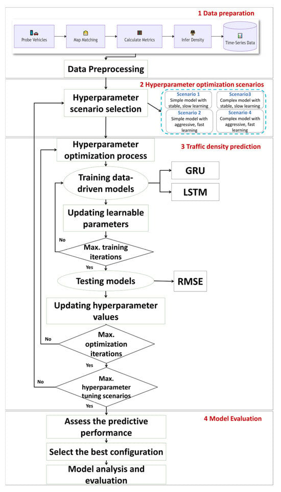
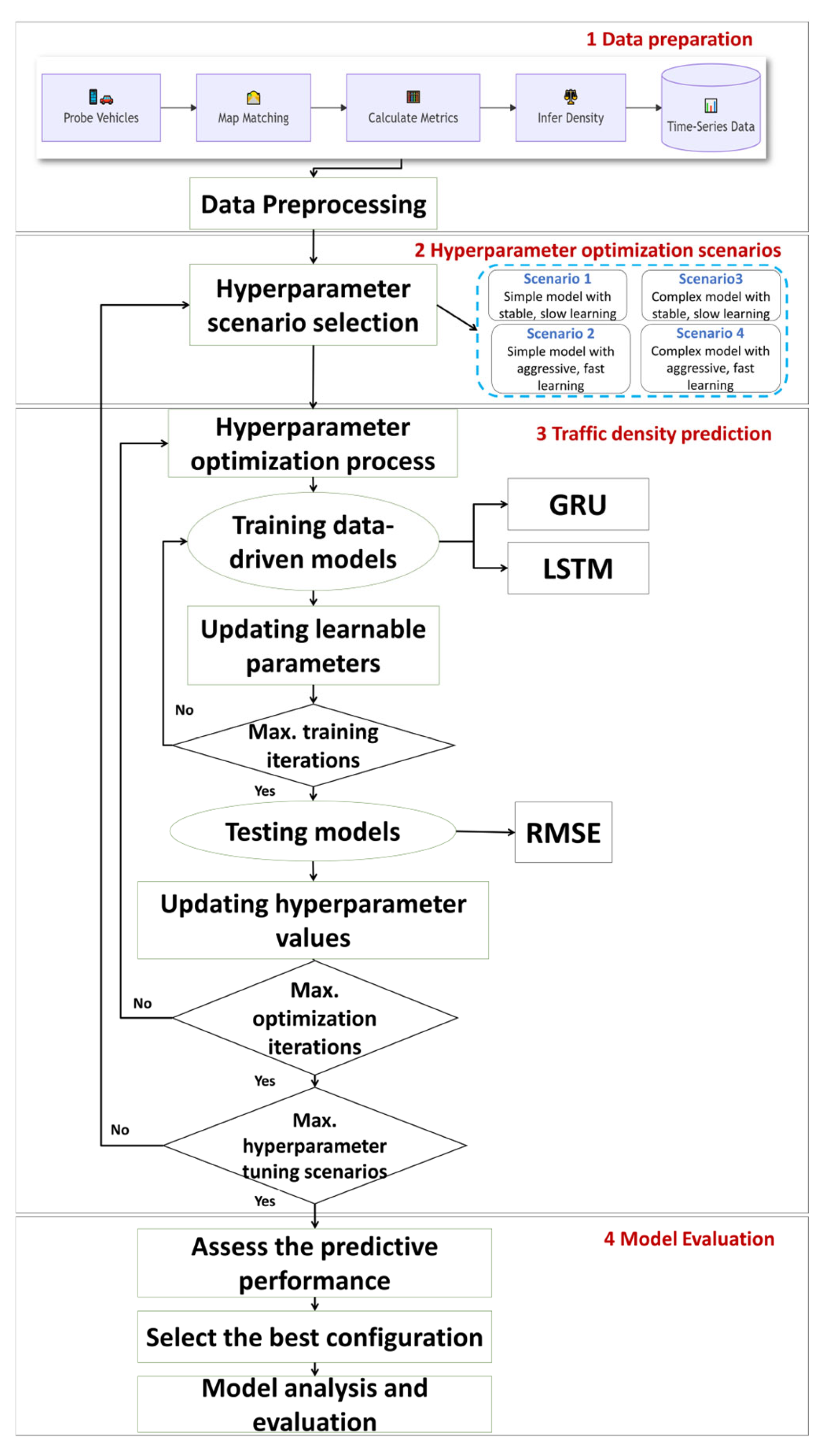
The proposed methodology, illustrated in Figure 1, outlines a structured framework for evaluating the influence of hyperparameter optimization on deep learning–based traffic flow prediction models. The methodology begins with the preprocessing of time-series traffic data, including probe-vehicle acquisition, map matching, metric computation, and flow inference. Building on this foundation, the methodology introduces a systematic hyperparameter optimization process aimed at identifying the most effective model configuration for traffic-flow forecasting. To achieve this, a Bayesian optimization framework was employed to efficiently explore the hyperparameter space across a set of predefined scenarios. These scenarios were designed to capture different combinations of model complexity and learning behavior, with particular emphasis on key factors such as the number of hidden units, training duration, initial learning rate, and learning-rate decay.

Figure 1. The proposed methodology for optimizing and evaluating GRU and LSTM for traffic flow estimation.

GRU and LSTM architectures are the main parts of the proposed predictive modeling approach. They are chosen because they have been shown to be able to find complex temporal dependencies in time-series data. GRU and LSTM were iteratively trained, with learnable parameters updated until the maximum number of training epochs was reached. Model performance was evaluated using RMSE to ensure an interpretable measure of predictive accuracy in the units of traffic flow. The hyperparameter optimization procedure relied on repeated cycles of sampling, training, and testing to guide subsequent hyperparameter selections. Once the maximum optimization iterations and scenario evaluations were completed, predictive performance was assessed across all configurations. The model achieving the lowest RMSE on the validation set was selected for final testing and a comprehensive performance review, confirming its suitability for the intended prediction task and demonstrating its potential applicability to broader traffic-management contexts.

3.1. Dataset Preparation

The dataset used in this study was obtained from the TomTom Junction Analytics platform, which provides high-resolution, real-time traffic monitoring data. Traffic conditions were recorded at the Globe Roundabout (“Dawar Al Kura Al Ardiyah”) in Jeddah, Saudi Arabia, during March 2025 (location link: https://maps.app.goo.gl/sEADt97byqK6PxR8A) (accessed on 1 December 2025). The platform logs traffic metrics at one-minute intervals, including congestion levels and traffic load, thereby capturing the dynamic flow of vehicles through the junction. This high temporal resolution enables a detailed examination of short-term fluctuations in traffic flow and offers a solid foundation for building reliable predictive models. The prediction task in this study aims to forecast hourly traffic volume (volumePerHour). Although raw data are collected at one-minute resolution, the target variable is constructed as the aggregated hourly traffic volume, while minute-level operational indicators are used as explanatory inputs.

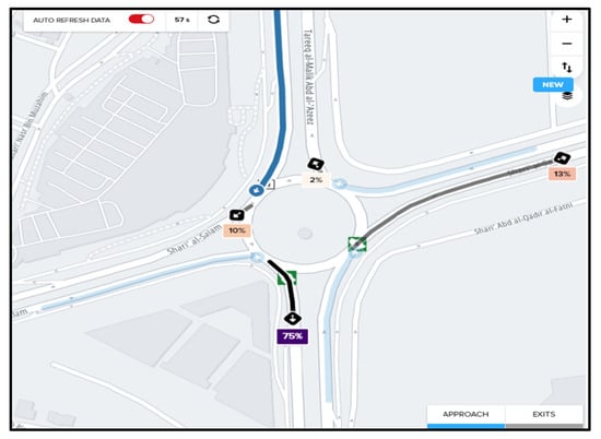
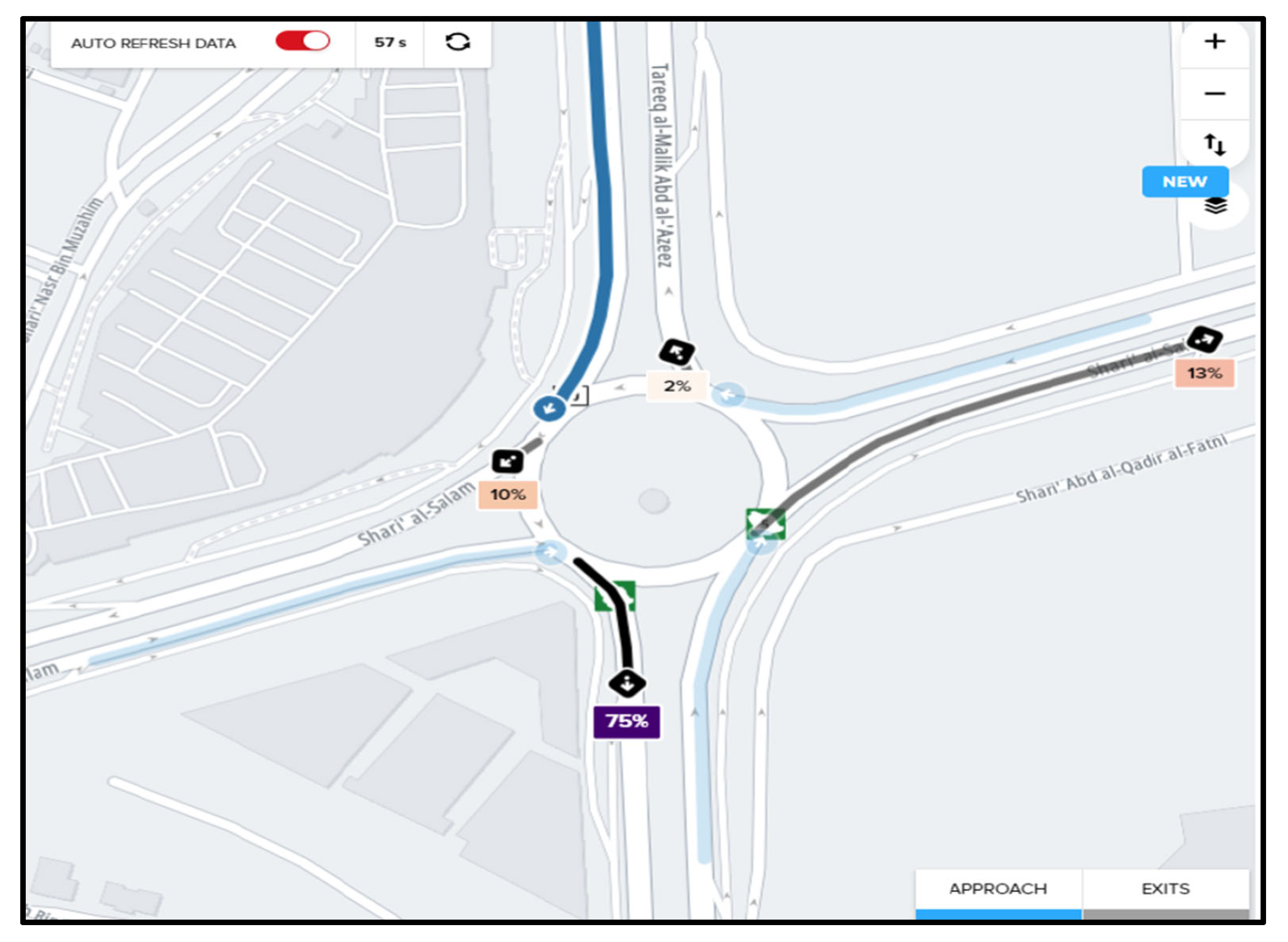
The analysis in this paper focuses specifically on the southern approach of the roundabout, shown in Figure 2. This segment, which is identified as “Prince Saud Al Faisal Road South Bound”, is a one-way corridor (FRC 3) approximately 275 m in length, channeling traffic northward toward the roundabout’s central circulation.

Figure 2. Visualization of the Southern Approach of the roundabout.

The raw dataset was first reorganized into a structured matrix format to ensure suitability for analysis. Traffic measurements were aggregated into hourly averages while retaining the original one-minute resolution, striking an effective balance between data granularity and computational efficiency. The dataset was first examined for completeness and consistency. No missing values were detected in the retrieved records, ensuring temporal continuity of the traffic measurements. Duplicate entries were removed where necessary to prevent redundancy. All numerical variables were subsequently standardized using Z-score normalization to ensure consistent scale across features and to facilitate stable and efficient model convergence during training.

Following preprocessing, the dataset was divided into two subsets to support model development and evaluation. To avoid data leakage, the dataset was split chronologically, where the first 80% of observations were used for training and validation, and the remaining 20% were reserved strictly for testing. The 80/20 train–test split was selected to balance model learning capacity and generalization assessment. This proportion is widely adopted in time-series deep learning studies and provides sufficient data for parameter learning while reserving an adequate unseen segment for robust performance evaluation. Within the training set, a validation subset was internally extracted to guide the Bayesian optimization process. Due to the temporal dependency structure of traffic time-series data, k-fold cross-validation was not employed, as it may introduce data leakage across sequential intervals. Instead, a temporally consistent validation split was adopted to preserve chronological order and ensure realistic forecasting evaluation. Hyperparameter optimization was conducted exclusively on the training set using internal validation.

This systematic preparation ensured that the dataset was both reliable and robust, meeting the necessary criteria for developing accurate traffic prediction models and contributing to improved traffic management strategies.

3.2. The Proposed Traffic Flow Prediction Methods

3.2.1. The GRU Model

The GRU is an advanced recurrent neural network architecture designed to address the limitations of traditional RNNs, particularly their difficulty in capturing long-range temporal dependencies. Introduced by [61], GRUs employ a gating mechanism that regulates the flow of information within the network, effectively mitigating the vanishing gradient problem while maintaining computational efficiency. The proposed traffic flow prediction model adopts a GRU-based architecture composed of four key components:

• Input Layer: This layer receives numFeature input features, incorporating relevant traffic variables such as historical flow values, vehicle flow rates, temporal indicators (e.g., time of day and day of week), and environmental conditions.
• GRU Layer: Serving as the core temporal processing stage, this layer consists of multiple hidden units that analyze sequential data. Through its gating mechanisms, the GRU captures complex, nonlinear temporal dependencies essential for modeling traffic behavior.
• Fully Connected Layer: A dense layer that transforms the high-dimensional feature representations produced by the GRU layer into the desired output dimension, generating the predicted traffic flow.
• Output Layer: This layer uses a linear activation function to produce continuous-valued predictions, optimized using the mean squared error (MSE) loss function, which is appropriate for regression tasks.

Mathematically, the GRU’s internal operations are governed by two primary gates, the update gate and the reset gate, which collectively determine how information is preserved or replaced across time steps. Let $x_t$ denote the input vector at time step $t$, and $h_{t-1}$ the previous hidden state. The GRU computes its hidden dynamics as follows:

$$z_t= \sigma \left( W_z \cdot {[h_{t-1},x}_t]+ b_z\right)$$

(1)

$$r_t=\sigma \left( W_r \cdot {[h_{t-1},x}_t]+b_r\right)$$

(2)

$${\tilde{h}}_t=tanh\left( W_h \cdot [r_t\odot {h_{t-1},x}_t]+b_h\right)$$

(3)

$$h_t=\left(1-z_t\right)\odot h_{t-1}+z_t\odot {\tilde{h}}_t$$

(4)

where $\sigma$ denotes the sigmoid activation function, $\odot$ represents the Hadamard (element-wise) product, and $W$ and $b$ refer to the learnable weight matrices and bias vectors, respectively. The update gate $z_t$ in Equation (1) regulates how much of the previous hidden state $h_{t-1}$ should be preserved, thereby balancing long-term contextual information with newly received input. As shown in Equations (2) and (3), the reset gate $r_t$ determines the extent to which the preceding hidden state contributes to the candidate activation ${\tilde{h}}_t$. This mechanism enables the network to selectively discard outdated or irrelevant temporal information. Together, these gating operations allow the GRU to retain meaningful long-term dependencies while efficiently integrating new input patterns. Such properties make the GRU particularly well-suited for traffic flow prediction, where both short-term fluctuations and historical trends influence future traffic states. The final hidden state $h_t$ produced at the last time step encapsulates the learned temporal representation of the entire input sequence and is passed to the fully connected layer to generate the final prediction (Equation (4)). This architecture effectively captures the complex temporal dynamics of traffic flow while remaining computationally efficient compared to more resource-intensive recurrent models.

3.2.2. The LSTM Model

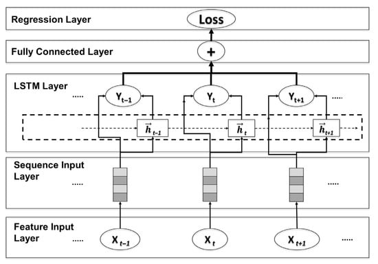
The proposed LSTM-based traffic flow prediction model leverages current traffic conditions by incorporating information extracted from previous time steps. As illustrated in Figure 3, the predictive network consists of five sequential layers. The first layer is a sequence input layer that feeds the input features into the deep learning architecture. This is followed by an LSTM layer, which is designed to effectively capture long-term temporal dependencies in traffic patterns. A fully connected layer then maps the output of the LSTM layer to a single value representing the predicted hourly traffic flow. The fourth layer is a Rectified Linear Unit (ReLU) layer, which applies an element-wise activation, replacing negative values with zero to enhance model nonlinearity and stabilization. Finally, a regression layer computes the half-mean-squared-error loss, suitable for continuous-valued sequential prediction tasks.

Figure 3. The proposed LSTM predictive model structure.

The Uni-LSTM predictive architecture produces its output through a series of internal operations occurring at each hidden neuron. At every time step $t$, the LSTM unit receives three components: the current input $x_t$, the previous hidden state $h_{t-1}$, and the previous cell state $c_{t-1}$. The internal memory is regulated by three gates: the input gate ($i_t$), forget gate ($f_t$), and output gate ($o_t$) which collectively determine how information is stored, updated, or discarded over time. Specifically, the input gate controls the incorporation of new information into the memory cell, the forget gate determines which past information should be removed, and the output gate regulates the information that is exposed to the next layer [31]. All three gates employ the sigmoid activation function to generate values between 0 and 1, effectively operating as soft “open” or “closed” gates [62]. The gate dynamics at time step $t$ are defined as:

$$i_t= \sigma (W_i \left[h_{t-1},x_t\right]+ b_i)$$

(5)

$$f_t=\sigma (W_f \left[h_{t-1},x_t\right]+b_f)$$

(6)

$$o_t=\sigma (W_o \left[h_{t-1},x_t\right]+b_o)$$

(7)

where $\sigma$ is the sigmoid activation function; $W_i,W_f,W_o$ are the learnable weight matrices for the three gates; $h_{t-1}$ is the previous hidden state; $x_t$ is the input at time $t$; and $b_i,b_f,b_o$ are the corresponding bias terms. To update the memory cell, the LSTM employs the hyperbolic tangent (tanh) activation function, which produces the cell candidate ${\widehat{c}}_t$. The tanh function is particularly advantageous in deep architectures due to its ability to stabilize gradients during training [62]. The cell candidate (${\widehat{c}}_t$), updated cell state ($c_t$), and resulting hidden state ($h_t$) are computed as:

$${\widehat{c}}_t=tanh(W_c\left[h_{t-1},x_t\right]+b_c)$$

(8)

$$c_t=f_t\odot c_{t-1}+i_t\odot {\widehat{c}}_t$$

(9)

$$h_t=o_t\odot \mathrm{t}\mathrm{a}\mathrm{n}\mathrm{h}\left(c_t\right)$$

(10)

3.3. Hyperparameter Optimization

This study employs Bayesian optimization to tune the hyperparameters of the proposed deep learning predictive models, advancing beyond traditional approaches such as grid search, random search, and evolutionary algorithms [63]. Hyperparameters are high-level configuration settings that control the learning behavior of a model; they must be specified prior to training and cannot be inferred directly from the data. As a result, their initial selection plays a crucial role in determining the model’s overall predictive performance. Bayesian optimization was selected over evolutionary approaches such as Particle Swarm Optimization (PSO) and Genetic Algorithms (GAs) due to its sample efficiency and probabilistic modeling capability. Unlike grid or random search, Bayesian optimization constructs a surrogate probabilistic model—typically a Gaussian Process—to approximate the objective surface and guide the search toward promising regions. Compared to population-based evolutionary algorithms, Bayesian optimization generally requires fewer objective evaluations, which is particularly advantageous when model training is computationally expensive. Given the relatively low-dimensional hyperparameter space considered in this study, Bayesian optimization provides a principled balance between exploration and exploitation while maintaining computational feasibility.

To identify optimal hyperparameter values, the Bayesian optimization process utilizes the Expected-Improvement-Plus acquisition function, which is particularly effective at avoiding convergence to local minima [64]. The optimization procedure is executed for each configuration, with the objective of minimizing the RMSE. The objective function, expressed as evalError, evaluates the RMSE value $Y$ associated with traffic load prediction using a specific hyperparameter configuration $X$ within a defined search space $D$. The process begins with an initialization phase in which random hyperparameter values $X$ are sampled and their corresponding RMSE values $Y$ are computed. A Gaussian Process (GP) model is then fitted to approximate the relationship between $X$ and $Y$. At each iteration $t$, the acquisition function estimates the expected improvement of the objective function, after which a new hyperparameter set $X_{\mathrm{new}}$ is selected by maximizing this acquisition value. The resulting RMSE $Y_{\mathrm{new}}$ is subsequently evaluated. Upon completing all iterations, the configuration yielding the minimum RMSE is selected as the optimal model.

To comprehensively explore the hyperparameter space, four optimization scenarios were constructed, each designed to examine different aspects of model behavior and learning dynamics. As summarized in Table 1, the scenarios differ in three primary dimensions: model capacity, training duration, and learning rate strategy.

Table 1. Description of the proposed hyperparameter optimization scenarios.

Scenario	Model Capacity	Training Duration	Learning Rate Aggressiveness
1	Low to Moderate	Short to Moderate	Low Start, Cautious
2	Low to Moderate	Short to Moderate	High Start, Aggressive
3	High	Long	Low Start, Cautious
4	High	Long	High Start, Aggressive

• Scenario 1 adopts a conservative approach, pairing a low-to-moderate-capacity model with a cautious learning strategy. This configuration aims to produce robust yet potentially under-fitted solutions.
• Scenario 2 maintains the same model capacity but applies a more aggressive learning strategy to assess whether faster convergence can deliver strong performance without increased architectural complexity.
• Scenario 3 investigates high-capacity models trained for extended durations with a low learning rate, allowing the models to gradually capture more nuanced temporal patterns.
• Scenario 4 represents a high-risk, high-reward configuration that combines high model capacity with a fast learning rate, testing whether complex architectures can converge rapidly without sacrificing accuracy.

This systematic design ensures a comprehensive evaluation of how model complexity, training length, and optimization dynamics interact, ultimately supporting the development of more accurate and reliable traffic flow prediction models. These configurations were designed to emulate realistic operational constraints in practical traffic-management systems, where computational resources, convergence speed, and model complexity must be carefully balanced during real-world deployment.

3.4. Evaluation Metric

To measure the prediction performance accuracy, the predicted traffic load, obtained from the testing process is compared with the actual values using the Mean Square Error (MSE), Root Mean Square Error (RMSE), and Mean Absolute Errors (MAEs) calculated as follows:

$$MSE={\displaystyle \frac{{\sum }_{i=1}^N{(x_i-y_i)}^2}{N}}$$

(11)

$$RMSE=\sqrt{{\displaystyle \frac{{\sum }_{i=1}^N{(x_i-y_i)}^2}{N}}}$$

(12)

$$MAE={\displaystyle \frac{1}{N}}\times {\sum }_{i=1}^N|x_i-y_i|$$

(13)

in which x_i and y_i are the actual and predicted load values, respectively, and N is the total number of observations.

4. Results and Discussion

This section is organized into four parts. Section 4.1 presents the results of the Bayesian hyperparameter-optimization process. Section 4.2 discusses the optimal hyperparameter configurations obtained for both the LSTM and GRU models. In Section 4.3, the predictive outputs of the optimized models are compared with existing approaches proposed by [11].

To evaluate the proposed methodology, real-world traffic dataset is used. The dataset captures one-minute traffic conditions at the Globe Roundabout (“Dawar Al Kura Al Ardiyah”) in Jeddah, Saudi Arabia, throughout March 2025.

To guarantee reproducibility, all models were trained and validated in a uniform hardware and software setting, employing CPU-based computation (Intel^® Core™ i9-10900 @ 2.80 GHz) within the MATLAB R2024a framework. This setup made it easy to compare model efficiency and prediction accuracy directly, without any GPU-acceleration variables.

4.1. Impact of Hyperparameter Optimization

To comprehensively explore the hyperparameter space, the four optimization scenarios previously described in Section 3.1 were constructed, and these scenarios are summarized in Table 2. These scenarios were applied to both the LSTM and GRU prediction models. Preliminary computational experiments were conducted to determine the number of optimization iterations required for convergence. Based on these trials, each scenario was optimized over 100 iterations, ensuring sufficient exploration of the search space and reliable identification of the minimum-error configuration. Preliminary convergence diagnostics were conducted to assess the stability of the optimization process. It was observed that RMSE improvements plateaued between 80 and 95 iterations across scenarios. Therefore, 100 iterations were selected to ensure sufficient exploration of the hyperparameter space while avoiding unnecessary computational overhead. This choice aligns with common practice in Bayesian optimization applications for deep learning tuning.

Table 2. Hyperparameter Boundaries for Bayesian Optimization of LSTM and GRU Models.

Hyperparameter	Scenario 1		Scenario 2		Scenario 3		Scenario 4
	Min	Max	Min	Max	Min	Max	Min	Max
Number of hidden units	5	50	5	50	51	100	51	100
Number of epochs	5	50	5	50	51	100	51	100
Initial learn rate	1 × 10−4	0.01	1 × 10−2	0.1	1 × 10−4	0.01	1 × 10−2	0.1
Learn rate drop factor	1 × 10−2	0.5	1 × 10−2	0.5	1 × 10−2	0.5	1 × 10−2	0.5

The hyperparameter boundaries presented in Table 2 were determined based on three considerations:

• Preliminary pilot experiments conducted to identify stable training ranges.
• Commonly adopted parameter intervals reported in recent traffic forecasting studies (2022–2025).
• Computational feasibility constraints under a CPU-based training environment.

The selected ranges were intentionally structured to differentiate between low-to-moderate and high-capacity configurations, enabling systematic assessment of model complexity versus learning aggressiveness.

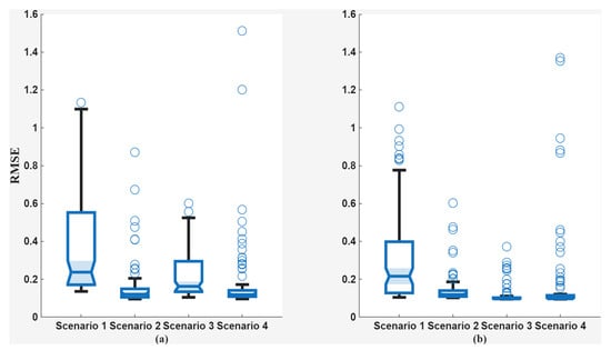
Figure 4a,b show the distribution of RMSE values across the 100 iterations for the four scenarios applied to both the LSTM and GRU models. In general, the GRU scenarios achieve lower median RMSE values than the LSTM ones. Scenario 1 shows the highest median RMSE for both models, which reflects the limitations of using low ranges for the initial learning rate, hidden units, and number of epochs.

Figure 4. RMSE values of the proposed optimized configurations. (a) LSTM Scenarios. (b) GRU Scenarios.

For the LSTM results in Figure 4a, Scenarios 2 and 4 perform noticeably better than Scenarios 1 and 3. This indicates that allowing higher initial learning rates during optimization plays an important role in improving accuracy, regardless of the other hyperparameter ranges. Scenarios 2 and 4 produce median RMSE values of 0.1211 and 0.119, with 10 and 16 outliers, respectively.

The GRU results in Figure 4b are more consistent across Scenarios 2, 3, and 4. Their median RMSE values are 0.1196, 0.09767, and 0.1002, which are relatively close, with 12, 17, and 19 outliers. These results highlight how changes in the hyperparameter ranges influence model accuracy and show that the GRU maintains stable performance across different optimization settings.

4.2. Best Configuration and Detailed Results

For each traffic flow prediction configuration described in Section 4.1, one hundred optimization iterations were conducted, and the iteration yielding the lowest RMSE was selected as the optimal configuration, i.e., the best combination of number of hidden units, epochs, initial learning rate, and learning rate drop factor to minimize the RMSE. Table 3 summarizes the hyperparameter values of the best-performing GRU and LSTM models.

Table 3. Hyperparameter values of the best model configuration.

Model	Scenario	Hyperparameter
		Number of Hidden Units	Number of Epochs	Initial Learn Rate	Learn Rate Drop Factor	RMSE
Optimized GRU	1	47	50	0.0097	0.0412	0.105
	2	49	50	0.0107	0.0136	0.103
	3	85	99	0.0066	0.0177	0.095
	4	51	100	0.0331	0.0808	0.095
Optimized LSTM	1	43	50	0.0100	0.0906	0.136
	2	8	49	0.0984	0.0113	0.096
	3	52	98	0.0099	0.0116	0.105
	4	51	92	0.0244	0.0417	0.097

The results indicate that the Optimized GRU generally outperforms the LSTM, achieving lower RMSE values in three of the four scenarios (1, 3, and 4). The lowest RMSE (0.0953) was recorded in GRU Scenarios 3 and 4, while LSTM demonstrated superior performance only in Scenario 2 with RMSE value of 0.0960, marginally surpassing the GRU (0.1026). These findings highlight that optimal model performance is scenario dependent.

The analysis of hyperparameters reveals several key insights: the number of hidden units varies widely from 8 to 85, showing no consistent pattern and indicating that optimal network complexity is highly specific to each scenario and model type, which reinforces the necessity of automated hyperparameter tuning. Regarding training duration, simpler scenarios (1 and 2) required only 50 epochs for convergence, while the more complex problems presented in Scenarios 3 and 4 needed a significantly higher number of epochs (92 to 100) to train properly. Finally, while the initial learning rates for all models fell within a standard range for the Adam optimizer, the learning rate drop factor exhibited considerable variability, with some models using a very gentle reduction and others applying a much more aggressive drop.

Based on the analysis of the four distinct forecasting tasks, Scenario 1 emerged as the most challenging for the LSTM model, which achieved its highest RMSE (0.1360), while the GRU handled it more effectively (0.1047); conversely, Scenarios 3 and 4 appeared to be the most amenable to modeling, as both architectures achieved their best and most consistent results there. When considering computational cost against performance, the GRU model in Scenario 3, with its large number of hidden units (85) and high epoch count (99), represents the most computationally expensive option, whereas the LSTM model in Scenario 2 stands out for its exceptional efficiency, achieving a stellar RMSE of 0.0960 with minimal resources—only 8 hidden units and 49 epochs—making it a highly efficient and high-performing model.

4.3. Comparison with Existing Approaches

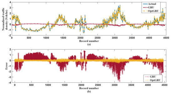
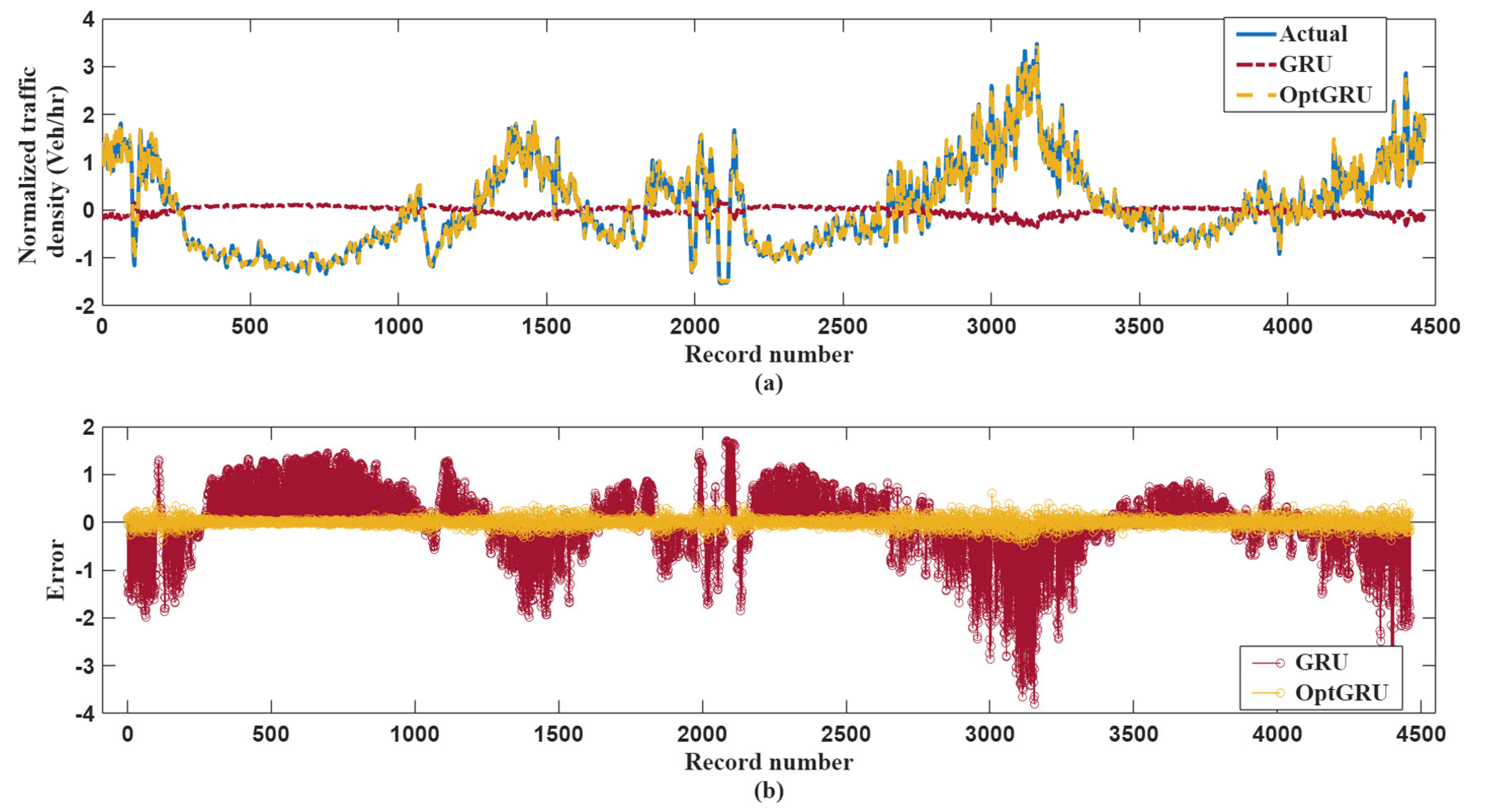
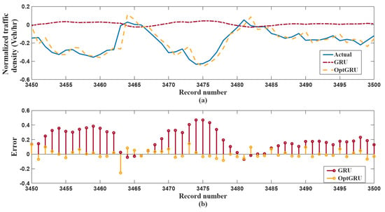
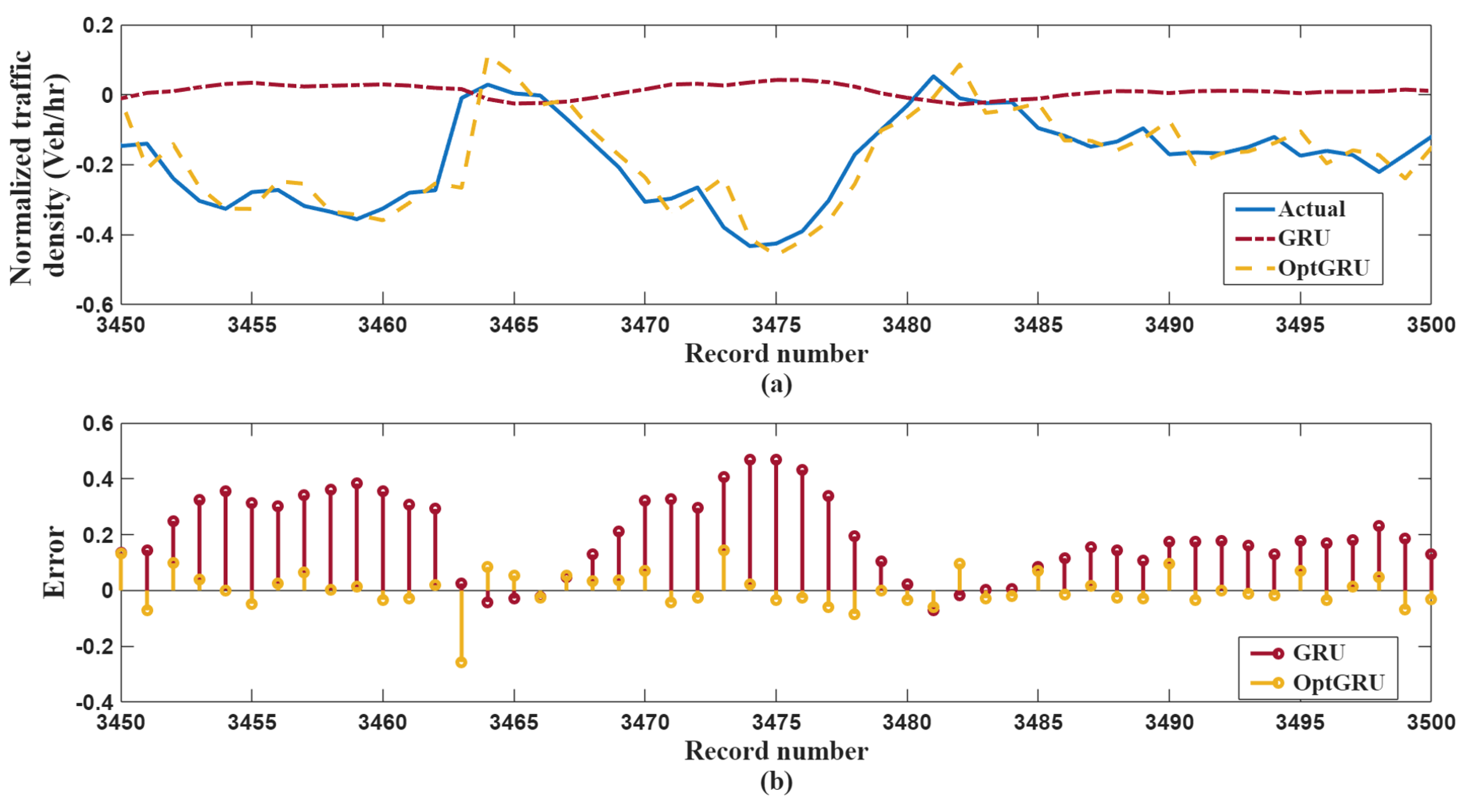
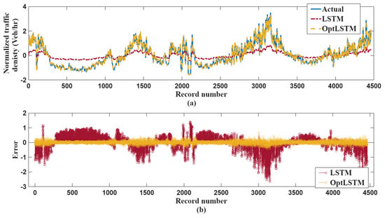
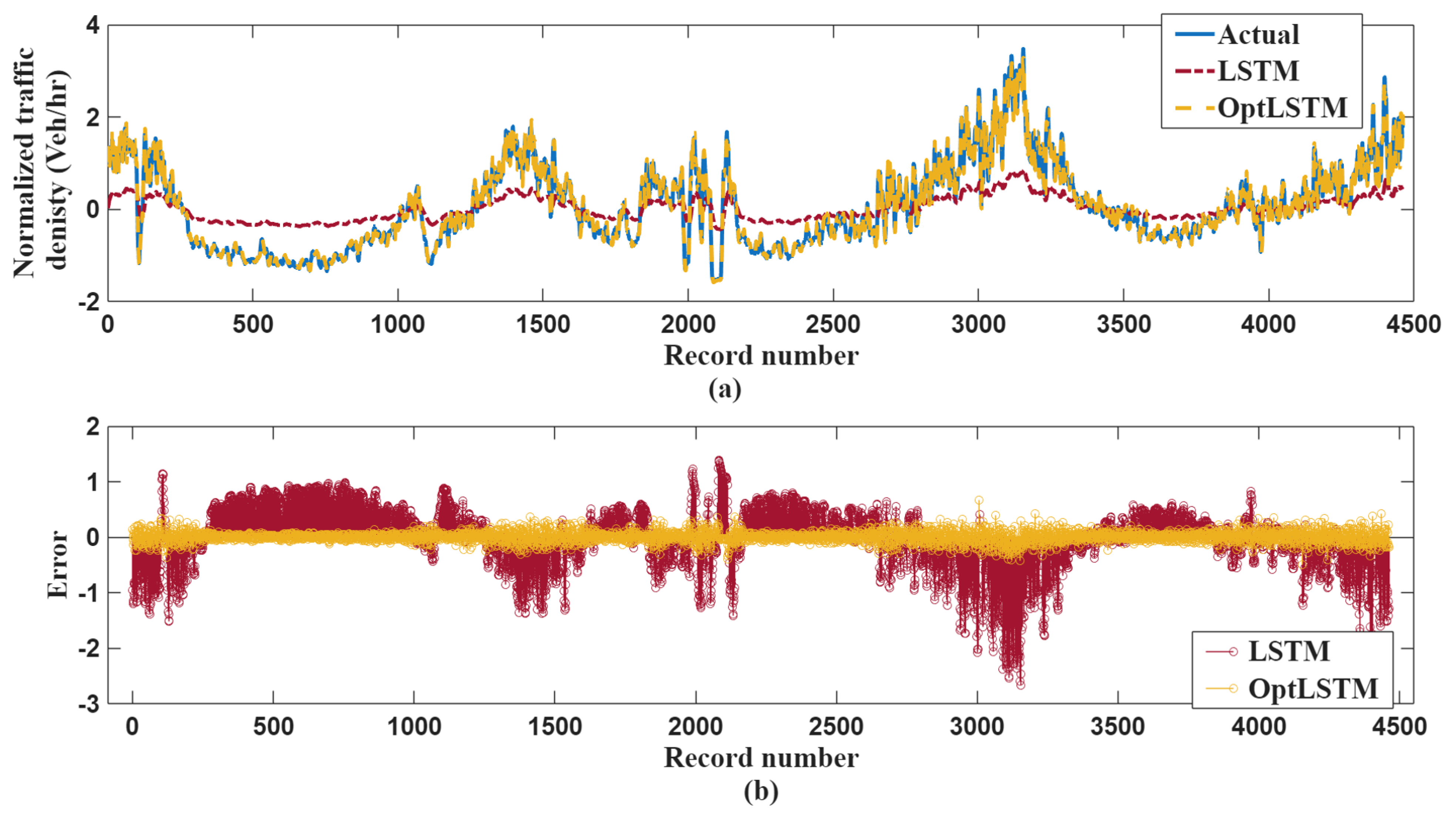
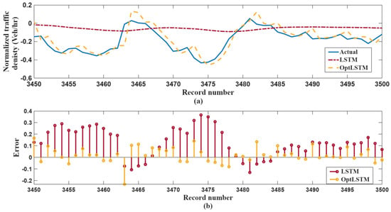
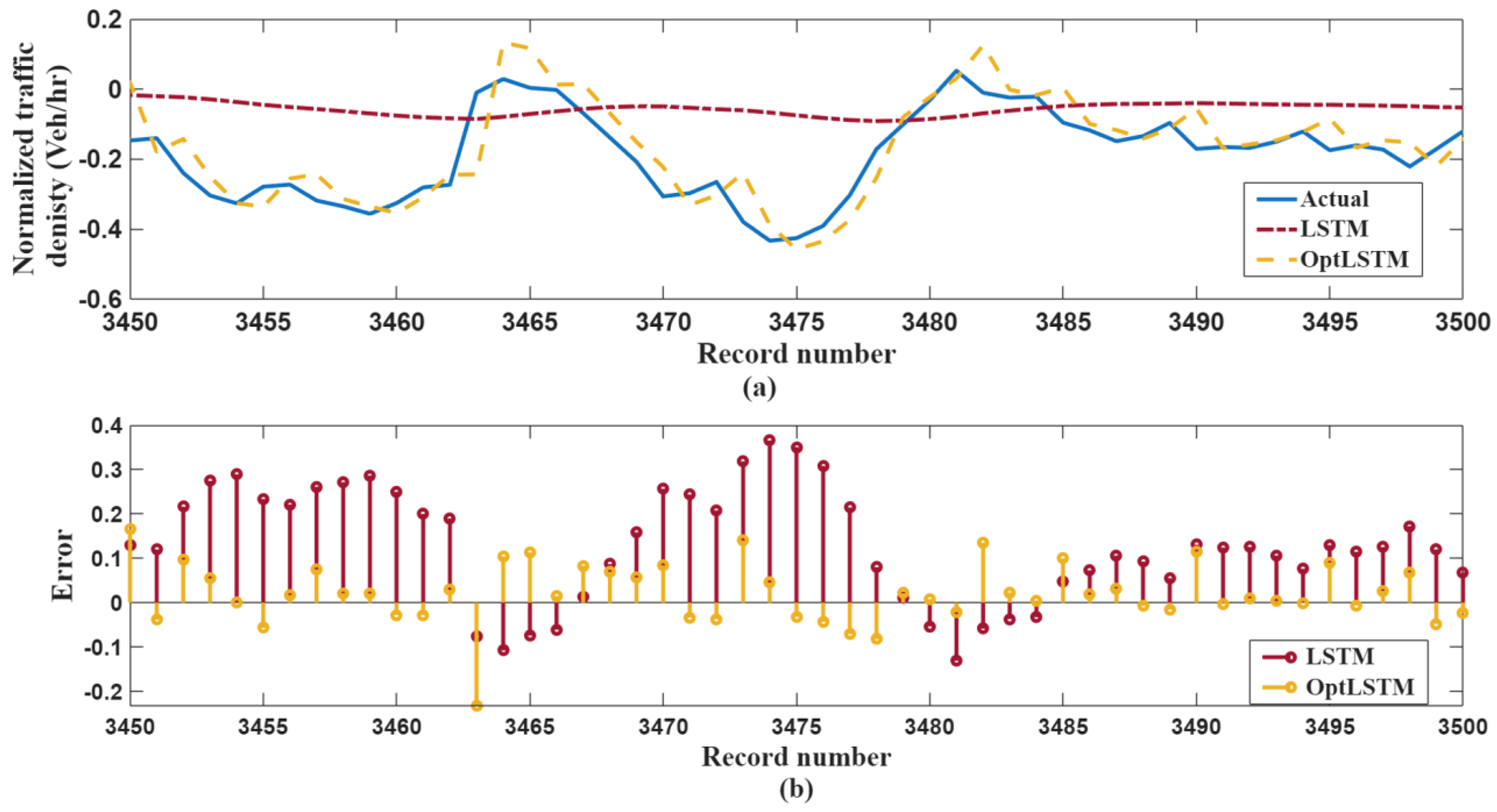
This section presents a comparative evaluation of the proposed optimized models, i.e., Opt-GRU and Opt-LSTM, against their baseline counterparts, i.e., GRU and LSTM, proposed by [11] and the observed traffic-flow data. Figure 5, Figure 6, Figure 7 and Figure 8 show time-series comparisons and point-wise error profiles for representative test intervals for Opt-GRU and Opt-LSTM, respectively while Table 4 summarizes standard error metrics (MSE, RMSE, MAE) for all comparative analyses.

Figure 5. Prediction performance and associated errors of the proposed OptGRU predictive model: (a) predicted and actual normalized traffic density; (b) prediction errors of GRU and OptGRU.

Figure 6. Prediction performance of the proposed OptGRU predictive model with corresponding errors over a 50-record resolution: (a) predicted and actual normalized traffic density; (b) prediction errors of GRU and OptGRU.

Figure 7. Prediction performance and associated errors of the proposed OptLSTM predictive model: (a) predicted and actual normalized traffic density; (b) prediction errors of LSTM and OptLSTM.

Figure 8. Prediction performance of the proposed OptLSTM predictive model with corresponding errors over a 50-record resolution: (a) predicted and actual normalized traffic density; (b) prediction errors of LSTM and OptLSTM.

Table 4. The prediction accuracy of the proposed optimized configurations.

Model	MSE	RMSE	MAE
GRU	0.938	0.969	0.779
Opt-GRU	0.009	0.095	0.067
LSTM	0.420	0.648	0.514
Opt-LSTM	0.009	0.096	0.069

Figure 5 compares the forecasting performance of the baseline GRU and the OptGRU in a representative test interval. Figure 5a displays the normalized observed series together with predictions from both models. Visually, the OptGRU predictions closely track the observations, accurately reproducing transient fluctuations and extreme values; by contrast, the baseline GRU shows larger deviations from the ground truth, particularly at peaks. This qualitative comparison indicates that the OptGRU model achieves a substantially better fit. Figure 5b presents the point-wise prediction errors for both models. The OptGRU error series exhibits markedly lower amplitude and variance and remains close to zero for the majority of the interval. In contrast, the baseline GRU error is larger and more volatile. These error profiles suggest that the optimization procedure reduces both the model’s variance and its stochastic error component without introducing a detectable systematic bias.

Overall, Figure 5 provides both visual and quantitative evidence that the proposed optimization yields a more accurate and reliable GRU-based predictor. The OptGRU effectively compensates for the baseline GRU’s deficiencies, improving fidelity to the measured signal and thereby increasing the model’s practical utility for traffic-flow forecasting.

Figure 6 presents a 48 h evaluation that extends the observations in Figure 5. Figure 6a highlights a smoothing bias in the baseline GRU: it tends to underestimate peaks and overestimate troughs, thereby attenuating the true amplitude of traffic fluctuations. The OptGRU, by contrast, closely follows sharp variations and peak events. Figure 6b shows the corresponding point-wise errors: the baseline GRU displays systematic, cycle-correlated errors indicative of persistent over- and under-prediction, whereas the OptGRU errors are substantially smaller and resemble unstructured noise centered near zero. Collectively, Figure 5 and Figure 6 demonstrate that hyperparameter optimization materially improves GRU performance, yielding greater accuracy and stability across both high- and low-traffic conditions.

Figure 7 presents a detailed comparison between the baseline LSTM and the Opt-LSTM under the same test conditions used for the GRU experiments. Figure 7a shows the observed traffic series together with the two model predictions. Both models capture the principal patterns and seasonal structure of the data; however, the Opt-LSTM predictions are visually indistinguishable from the ground truth, whereas the baseline LSTM exhibits a consistent smoothing bias—underestimating local maxima and overestimating local minima—and thus attenuates the amplitude of extreme events. Figure 7b displays the point-wise prediction errors. The baseline LSTM error series is characterized by large amplitudes and high variance, indicating substantial and structured inaccuracies. By contrast, the Opt-LSTM error remains tightly concentrated near zero with very low variance and appears as a thin, near-flat line relative to the baseline. This pattern indicates that the optimization procedure substantially reduced both systematic bias and random error magnitude, leaving only small residual noise.

Figure 8 provides a complementary 48 h diagnostic that reinforces the observations from Figure 7. Figure 8a again highlights the baseline LSTM’s smoothing shortfall and the Opt-LSTM’s close tracking of peaks and transitions. Figure 8b quantifies the contrast: the baseline LSTM error shows a pronounced cycle-related structure and considerable magnitude, whereas the Opt-LSTM error is negligible, unstructured, and consistent with low-variance random noise. The clear performance gap evidenced in Figure 7 and Figure 8 demonstrates that the applied optimization effectively mitigates internal limitations of the LSTM architecture and substantially enhances forecasting accuracy and stability.

Taken together, these results show that the Opt-LSTM reliably captures both extreme and transient traffic dynamics, supporting its suitability for practical time-series forecasting tasks. Moreover, the improvements observed for the LSTM parallel those reported for the GRU (Figure 5 and Figure 6), indicating that the optimization methodology generalizes across recurrent architectures.

As shown in Table 4, the results of the performance analysis demonstrate a considerable improvement in predictive accuracy resulting from hyperparameter optimization for both the GRU and LSTM frameworks. The baseline model for GRU (MSE: 0.938, RMSE: 0.969, MAE: 0.779) significantly lagged behind the baseline LSTM model (MSE: 0.420, RMSE: 0.648, MAE: 0.514), thereby illustrating the inherent advantage of the LSTM architecture in effectively capturing temporal dependencies within their conventional settings. Following the optimization process, both models revealed noteworthy improvements, with the Opt-GRU achieving a 99.03% reduction in MSE, while the Opt-LSTM demonstrated a 97.81% improvement. This optimization led to MAE values approximating 0.07 for each model, indicating a remarkable increase in predictive accuracy that renders both architectures suitable for applications in traffic forecasting.

Optimization results show that after optimization, both of the calibrated models perform at similar levels, with Opt-GRU achieving marginally better results (MSE: 0.00909, RMSE: 0.0953, MAE: 0.0673) compared to Opt-LSTM (MSE: 0.00921, RMSE: 0.0960, MAE: 0.0687). This small difference in performance indicates that careful adjustments of hyperparameters can optimally compensate for architectural limitations, allowing the computationally lean GRU to approach a performance level equivalent to that of the more computationally demanding LSTM. The results highlight that in traffic forecasting task settings, careful optimization of hyperparameters is more important than architecture selection, as both models achieved the desired accuracy suitable for practical application after proper tuning. This indicates that model selection decisions might favour low computationally costly models when proper optimization strategies are in place.

5. Conclusions

This study presented a systematic Bayesian hyperparameter optimization framework to enhance the predictive performance of GRU and LSTM models for short-term traffic flow forecasting at a signalized intersection. Using minute-level real-world traffic data from the Globe Roundabout in Jeddah, Saudi Arabia, the proposed methodology was rigorously evaluated under multiple optimization scenarios within a controlled computational environment.

The results demonstrate that hyperparameter optimization leads to substantial improvements in predictive accuracy for both architectures. The optimized GRU and LSTM models achieved RMSE values of approximately 0.095, representing reductions exceeding 85% relative to their unoptimized baselines. Visual and quantitative analyses confirmed that optimization effectively mitigates smoothing bias, improves the tracking of transient and extreme traffic fluctuations, and yields stable, low-variance residuals across different traffic conditions.

Comparative evaluation against existing baseline approaches showed that, after optimization, the GRU and LSTM models exhibit nearly equivalent performance, with the optimized GRU achieving marginally lower error metrics while maintaining lower computational complexity. These findings indicate that careful hyperparameter tuning can compensate for architectural limitations, enabling lightweight recurrent models to perform at a level comparable to more complex alternatives.

Future work may address several limitations of the present study. Incorporating exogenous factors such as weather conditions or special events, modeling spatial correlations across adjacent network links, and exploring attention mechanisms or hybrid architectures could further enhance predictive accuracy. Additionally, evaluating online or incremental learning strategies may improve adaptability under nonstationary traffic conditions. Expanding validation to multi-site and multi-season datasets, along with reporting uncertainty estimates or statistical significance measures, would strengthen the generalizability and real-world applicability of the findings.

References

- Pishue, B.; Kidd, J. 2024 INRIX Global Traffic Scorecard; Inrix: Washington, DC, USA, 2024. [Google Scholar]
- Schrank, D.; Albert, L.; Jha, K.; Eisele, B. 2023 Urban Mobility Report; Texas A&M Transportation Institute: Bryan, TX, USA, 2024. [Google Scholar]
- Dano, U.L.; AlQahtany, A.M. Issues Undermining Public Transport Utilization in Dammam City, Saudi Arabia: An Expert-Based Analysis. J. Sustain. Sci. Manag. 2019, 14, 155–169. [Google Scholar]
- Sibai, A.A. Bottleneck Traffic Creates a Heavy Loss of SR 81 Billion; Saudi Gazette: Riyadh, Saudi Arabia, 2011. [Google Scholar]
- Li, D.; Zhao, X.; Cao, P. An Enhanced Motorway Control System for Mixed Manual/Automated Traffic Flow. IEEE Syst. J. 2020, 14, 4726–4734. [Google Scholar] [CrossRef] [Scilit]
- Shi, X.W.; Zhu, W.X.; Wang, Q.Y.; Shao, S.Y. Modeling for Traffic Overflow Mechanism and Its Simulation on Urban Arterial Road. J. Shandong Univ. (Eng. Sci.) 2013, 43, 43–48. [Google Scholar]
- Ren, Y.; Wang, Y.; Yu, G.; Liu, H.; Xiao, L. An Adaptive Signal Control Scheme to Prevent Intersection Traffic Blockage. IEEE Trans. Intell. Transp. Syst. 2016, 18, 1519–1528. [Google Scholar] [CrossRef] [Scilit]
- Zhang, L.; Zhao, Q.; Wang, L. Research on Intersection Frequent Overflow Control Strategy Based on Wide-Area Radar Data. J. Adv. Transp. 2020, 2020, 9564329. [Google Scholar] [CrossRef] [Scilit]
- Zhu, R.W.; Wu, D.; Yang, Z. Triggering Conditions and Scheme Design of Queuing Overflow Control at Signalized Intersections. J. Wuhan Univ. Technol. (Transport. Sci. Eng.) 2018, 42, 971–976. [Google Scholar]
- Liang, Z.; Wang, R.; Zhan, X.; Hu, T.; Li, X.; Li, Y. The Two-Stage Prediction Method for Traffic Spillover Dissipation at Short-Distance Intersections Based on Bi-LSTM. Sci. Rep. 2025, 15, 22249. [Google Scholar] [CrossRef] [Scilit]
- Harrou, F.; Zeroual, A.; Kadri, F.; Sun, Y. Enhancing Road Traffic Flow Prediction with Improved Deep Learning Using Wavelet Transforms. Results Eng. 2024, 23, 102342. [Google Scholar] [CrossRef] [Scilit]
- Abohashima, H.; Gheith, M.; Eltawil, A. A Proposed IoT Based Smart Traffic Lights Control System within a V2X Framework. In Proceedings of the 2020 2nd Novel Intelligent and Leading Emerging Sciences Conference (NILES), Giza, Egypt, 24–26 October 2020; Volume 2020, pp. 338–343. [Google Scholar] [CrossRef] [Scilit]
- Ma, X.; Tao, Z.; Wang, Y.; Yu, H.; Wang, Y. Long Short-Term Memory Neural Network for Traffic Speed Prediction Using Remote Microwave Sensor Data. Transp. Res. Part C Emerg. Technol. 2015, 54, 187–197. [Google Scholar] [CrossRef] [Scilit]
- Liao, S.; Chen, J.; Hou, J.; Xiong, Q.; Wen, J. Deep Convolutional Neural Networks with Random Subspace Learning for Short-Term Traffic Flow Prediction with Incomplete Data. In Proceedings of the 2018 International Joint Conference on Neural Networks (IJCNN), Rio de Janeiro, Brazil, 8–13 July 2018; IEEE: New York, NY, USA, 2018; pp. 1–6. [Google Scholar]
- Perera, L.P.; Soares, C.G. Ocean Vessel Trajectory Estimation and Prediction Based on Extended Kalman Filter. In Proceedings of the Second International Conference on Adaptive and Self-Adaptive Systems and Applications, Lisbon, Portugal, 21–26 November 2010; Citeseer: Princeton, NJ, USA, 2010; pp. 14–20. [Google Scholar]
- Yang, G.; Xv, R.; Qing, M.; Zheng, K.L.; Zhang, B. Short-Term Traffic Volume Forecasting Based on ARMA and Kalman Filter. J. Zhengzhou Univ. (Eng. Sci.) 2017, 38, 36–40. [Google Scholar]
- Okutani, I.; Stephanedes, Y.J. Dynamic Prediction of Traffic Volume through Kalman Filtering Theory. Transp. Res. Part B Methodol. 1984, 18, 1–11. [Google Scholar] [CrossRef] [Scilit]
- Abduljabbar, R.; Dia, H.; Liyanage, S. Machine Learning Models for Traffic Prediction on Arterial Roads Using Traffic Features and Weather Information. Appl. Sci. 2024, 14, 11047. [Google Scholar] [CrossRef] [Scilit]
- Harrou, F.; Zeroual, A.; Hittawe, M.M.; Sun, Y. Road Traffic Modeling and Management: Using Statistical Monitoring and Deep Learning; Elsevier: Amsterdam, The Netherlands, 2021; ISBN 0128234334. [Google Scholar]
- Csikós, A.; Viharos, Z.J.; Kis, K.B.; Tettamanti, T.; Varga, I. Traffic Speed Prediction Method for Urban Networks—An ANN Approach. In Proceedings of the 2015 International Conference on Models and Technologies for Intelligent Transportation Systems (MT-ITS), Budapest, Hungary, 3–5 June 2015; IEEE: New York, NY, USA, 2015; pp. 102–108. [Google Scholar]
- Zhang, L.; Liu, Q.; Yang, W.; Wei, N.; Dong, D. An Improved K-Nearest Neighbor Model for Short-Term Traffic Flow Prediction. Procedia-Soc. Behav. Sci. 2013, 96, 653–662. [Google Scholar] [CrossRef] [Scilit]
- Castro-Neto, M.; Jeong, Y.-S.; Jeong, M.-K.; Han, L.D. Online-SVR for Short-Term Traffic Flow Prediction under Typical and Atypical Traffic Conditions. Expert Syst. Appl. 2009, 36, 6164–6173. [Google Scholar] [CrossRef] [Scilit]
- Sun, S.; Zhang, C.; Yu, G. A Bayesian Network Approach to Traffic Flow Forecasting. IEEE Trans. Intell. Transp. Syst. 2006, 7, 124–132. [Google Scholar] [CrossRef] [Scilit]
- Medina-Salgado, B.; Sánchez-DelaCruz, E.; Pozos-Parra, P.; Sierra, J.E. Urban Traffic Flow Prediction Techniques: A Review. Sustain. Comput. Inform. Syst. 2022, 35, 100739. [Google Scholar] [CrossRef] [Scilit]
- Fang, W.; Zhuo, W.; Song, Y.; Yan, J.; Zhou, T.; Qin, J. Δfree-LSTM: An Error Distribution Free Deep Learning for Short-Term Traffic Flow Forecasting. Neurocomputing 2023, 526, 180–190. [Google Scholar] [CrossRef] [Scilit]
- Chang, L.; Ma, C.; Sun, K.; Qu, Z.; Ren, C. Enhanced Road Information Representation in Graph Recurrent Network for Traffic Speed Prediction. IET Intell. Transp. Syst. 2023, 17, 1434–1453. [Google Scholar] [CrossRef] [Scilit]
- Diehl, F.; Brunner, T.; Le, M.T.; Knoll, A. Graph Neural Networks for Modelling Traffic Participant Interaction. In Proceedings of the 2019 IEEE Intelligent Vehicles Symposium (IV), Paris, France, 9–12 June 2019; IEEE: New York, NY, USA, 2019; pp. 695–701. [Google Scholar]
- Toncharoen, R.; Piantanakulchai, M. Traffic State Prediction Using Convolutional Neural Network. In Proceedings of the 2018 15th International Joint Conference on Computer Science and Software Engineering (JCSSE), Nakhonpathom, Thailand, 11–13 July 2018; IEEE: New York, NY, USA, 2018; pp. 1–6. [Google Scholar]
- Fu, R.; Zhang, Z.; Li, L. Using LSTM and GRU Neural Network Methods for Traffic Flow Prediction. In Proceedings of the 2016 31st Youth Academic Annual Conference of Chinese Association of Automation (YAC), Wuhan, China, 11–13 November 2016; IEEE: New York, NY, USA, 2016; pp. 324–328. [Google Scholar]
- Katambire, V.N.; Musabe, R.; Uwitonze, A.; Mukanyiligira, D. Forecasting the Traffic Flow by Using ARIMA and LSTM Models: Case of Muhima Junction. Forecasting 2023, 5, 616–628. [Google Scholar] [CrossRef] [Scilit]
- Hochreiter, S.; Schmidhuber, J. Long Short-Term Memory. Neural Comput. 1997, 9, 1735–1780. [Google Scholar] [CrossRef] [Scilit]
- Mao, Y.; Qin, G.; Ni, P.; Liu, Q. Analysis of Road Traffic Speed in Kunming Plateau Mountains: A Fusion PSO-LSTM Algorithm. Int. J. Urban Sci. 2022, 26, 87–107. [Google Scholar] [CrossRef] [Scilit]
- Guo, C.; Zhu, J.; Wang, X. Mvhs-Lstm: The Comprehensive Traffic Flow Prediction Based on Improved Lstm via Multiple Variables Heuristic Selection. Appl. Sci. 2024, 14, 2959. [Google Scholar] [CrossRef] [Scilit]
- Sadeghi-Niaraki, A.; Mirshafiei, P.; Shakeri, M.; Choi, S.-M. Short-Term Traffic Flow Prediction Using the Modified Elman Recurrent Neural Network Optimized through a Genetic Algorithm. IEEE Access 2020, 8, 217526–217540. [Google Scholar] [CrossRef] [Scilit]
- Zhang, J.; Qu, S.; Zhang, Z.; Cheng, S. Improved Genetic Algorithm Optimized LSTM Model and Its Application in Short-Term Traffic Flow Prediction. PeerJ Comput. Sci. 2022, 8, e1048. [Google Scholar] [CrossRef] [Scilit]
- Alghamdi, T.; Elgazzar, K.; Bayoumi, M.; Sharaf, T.; Shah, S. Forecasting Traffic Congestion Using ARIMA Modeling. In Proceedings of the 2019 15th International Wireless Communications & Mobile Computing Conference (IWCMC), Tangier, Morocco, 24–28 June 2019; IEEE: New York, NY, USA, 2019; pp. 1227–1232. [Google Scholar]
- Alam, I.; Farid, D.M.; Rossetti, R.J.F. The Prediction of Traffic Flow with Regression Analysis. In Emerging Technologies in Data Mining and Information Security, Proceedings of IEMIS 2018, West Bengal, Kolkata, 23–25 February 2018; Springer: Berlin/Heidelberg, Germany, 2018; Volume 2, pp. 661–671. [Google Scholar]
- Guo, J.; Huang, W.; Williams, B.M. Adaptive Kalman Filter Approach for Stochastic Short-Term Traffic Flow Rate Prediction and Uncertainty Quantification. Transp. Res. Part C Emerg. Technol. 2014, 43, 50–64. [Google Scholar] [CrossRef] [Scilit]
- Run, L.; Min, L.X.; Lu, Z.X. Research and Comparison of ARIMA and Grey Prediction Models for Subway Traffic Forecasting. In Proceedings of the 2020 International Conference on Intelligent Computing, Automation and Systems (ICICAS), Chongqing, China, 11–13 December 2020; IEEE: New York, NY, USA, 2020; pp. 63–67. [Google Scholar]
- Vidya, G.S.; Hari, V.S.; Shivasagaran, S. Estimation of Passenger Flow in a Bus Route Using Kalman Filter. In Proceedings of the 2020 6th International Conference on Advanced Computing and Communication Systems (ICACCS), Coimbatore, India, 6–7 March 2020; IEEE: New York, NY, USA, 2020; pp. 1248–1251. [Google Scholar]
- Lim, J.; Lee, J.; An, C.; Park, E. Enhancing Real-time Traffic Volume Prediction: A Two-step Approach of Object Detection and Time Series Modelling. IET Intell. Transp. Syst. 2024, 18, 2744–2758. [Google Scholar] [CrossRef] [Scilit]
- Xu, S.; Sun, C.; Liu, N. Road Congestion and Air Pollution—Analysis of Spatial and Temporal Congestion Effects. Sci. Total Environ. 2024, 945, 173896. [Google Scholar] [CrossRef] [Scilit]
- Wu, K.; Ding, J.; Lin, J.; Zheng, G.; Sun, Y.; Fang, J.; Xu, T.; Zhu, Y.; Gu, B. Big-Data Empowered Traffic Signal Control Could Reduce Urban Carbon Emission. Nat. Commun. 2025, 16, 1987. [Google Scholar] [CrossRef] [Scilit]
- Alrayes, F.S.; Wiwatanapataphee, B.; Wu, Y.H. Towards Green Innovation in Smart Cities: Leveraging Traffic Flow Prediction with Machine Learning Algorithms for Sustainable Transportation Systems. Sustainability 2024, 16, 251. [Google Scholar]
- Chen, R.; Liang, C.-Y.; Hong, W.-C.; Gu, D.-X. Forecasting Holiday Daily Tourist Flow Based on Seasonal Support Vector Regression with Adaptive Genetic Algorithm. Appl. Soft Comput. 2015, 26, 435–443. [Google Scholar] [CrossRef] [Scilit]
- Zivot, E.; Wang, J. Modeling Financial Time Series with S-Plus®; Springer: Berlin/Heidelberg, Germany, 2006. [Google Scholar]
- Modi, Y.; Teli, R.; Mehta, A.; Shah, K.; Shah, M. A Comprehensive Review on Intelligent Traffic Management Using Machine Learning Algorithms. Innov. Infrastruct. Solut. 2022, 7, 128. [Google Scholar]
- Zhang, Y.; Xie, Y. Forecasting of Short-Term Freeway Volume with v-Support Vector Machines. Transp. Res. Rec. 2007, 2024, 92–99. [Google Scholar] [CrossRef] [Scilit]
- Feng, X.; Ling, X.; Zheng, H.; Chen, Z.; Xu, Y. Adaptive Multi-Kernel SVM with Spatial–Temporal Correlation for Short-Term Traffic Flow Prediction. IEEE Trans. Intell. Transp. Syst. 2018, 20, 2001–2013. [Google Scholar] [CrossRef] [Scilit]
- Singh, V.; Sahana, S.K.; Bhattacharjee, V. A Novel CNN-GRU-LSTM Based Deep Learning Model for Accurate Traffic Prediction. Discov. Comput. 2025, 28, 38. [Google Scholar]
- Goodfellow, I.; Bengio, Y.; Courville, A.; Bengio, Y. Deep Learning; MIT Press Cambridge: Cambridge, UK, 2016; Volume 1. [Google Scholar]
- Bruna, J.; Zaremba, W.; Szlam, A.; LeCun, Y. Spectral Networks and Locally Connected Networks on Graphs. arXiv 2013, arXiv:1312.6203. [Google Scholar]
- Cui, Z.; Ke, R.; Pu, Z.; Wang, Y. Deep Bidirectional and Unidirectional LSTM Recurrent Neural Network for Network-Wide Traffic Speed Prediction. arXiv 2018, arXiv:1801.02143. [Google Scholar]
- Wang, H.; Wei, X.; Yao, J.; Zhang, Y. Traffic Flow Prediction Using Machine Learning Methods. In Proceedings of the 2021 3rd International Conference on Machine Learning, Big Data and Business Intelligence (MLBDBI), Taiyuan, China, 3–5 December 2021; IEEE: New York, NY, USA, 2021; pp. 30–35. [Google Scholar]
- Yao, E.; Zhang, L.; Li, X.; Yun, X. Traffic Forecasting of Back Servers Based on ARIMA-LSTM-CF Hybrid Model. Int. J. Comput. Intell. Syst. 2023, 16, 65. [Google Scholar] [CrossRef] [Scilit]
- Lin, K.-Y.; Liu, P.-Y.; Wang, P.-K.; Hu, C.-L.; Cai, Y. Predicting Road Traffic Risks with CNN-and-LSTM Learning over Spatio-Temporal and Multi-Feature Traffic Data. In Proceedings of the 2023 IEEE International Conference on Software Services Engineering (SSE), Chicago, IL, USA, 2–8 July 2023; IEEE: New York, NY, USA, 2023; pp. 305–311. [Google Scholar]
- Yang, H.; Wang, M.; Li, G. A Combined Prediction Model Based on Secondary Decomposition and Intelligence Optimization for Carbon Emission. Appl. Math. Model. 2023, 121, 484–505. [Google Scholar] [CrossRef] [Scilit]
- Lu, W.; Hu, Y.; Chen, W.; Qin, Y.; Wu, C.; He, X. Traffic Flow Prediction for Highway Vehicle Detectors through Decomposition and Machine Learning. Transp. Lett. 2025, 17, 260–280. [Google Scholar]
- Rui, Y.; Gong, Y.; Zhao, Y.; Luo, K.; Lu, W. Predicting Traffic Flow Parameters for Sustainable Highway Management: An Attention-Based EMD–BiLSTM Approach. Sustainability 2023, 16, 190. [Google Scholar] [CrossRef] [Scilit]
- Atef, S.; Eltawil, A.B. Assessment of Stacked Unidirectional and Bidirectional Long Short-Term Memory Networks for Electricity Load Forecasting. Electr. Power Syst. Res. 2020, 187, 106489. [Google Scholar] [CrossRef] [Scilit]
- Cho, K.; Van Merriënboer, B.; Gulcehre, C.; Bahdanau, D.; Bougares, F.; Schwenk, H.; Bengio, Y. Learning Phrase Representations Using RNN Encoder-Decoder for Statistical Machine Translation. In Proceedings of the EMNLP 2014—2014 Conference on Empirical Methods in Natural Language Processing, Doha, Qatar, 25–29 October 2014; pp. 1724–1734. [Google Scholar] [CrossRef] [Scilit]
- Nwankpa, C.; Ijomah, W.; Gachagan, A.; Marshall, S. Activation Functions: Comparison of Trends in Practice and Research for Deep Learning. arXiv 2018, arXiv:1811.03378. [Google Scholar] [CrossRef] [Scilit]
- Snoek, J.; Larochelle, H.; Adams, R.P. Practical Bayesian Optimization of Machine Learning Algorithms. In Advances in Neural Information Processing Systems 25; Pereira, F., Burges, C.J.C., Bottou, L., Weinberger, K.Q., Eds.; Curran Associates, Inc.: New York, NY, USA, 2012; pp. 2951–2959. [Google Scholar]
- Berk, J.; Nguyen, V.; Gupta, S.; Rana, S.; Venkatesh, S. Exploration Enhanced Expected Improvement for Bayesian Optimization. In Proceedings of the Machine Learning and Knowledge Discovery in Databases; Berlingerio, M., Bonchi, F., Gärtner, T., Hurley, N., Ifrim, G., Eds.; Springer International Publishing: Cham, Switzerland, 2019; pp. 621–637. [Google Scholar]
Disclaimer/Publisher’s Note: The statements, opinions and data contained in all publications are solely those of the individual author(s) and contributor(s) and not of MDPI and/or the editor(s). MDPI and/or the editor(s) disclaim responsibility for any injury to people or property resulting from any ideas, methods, instructions or products referred to in the content. |
© 2026 by the authors. Published by MDPI on behalf of the International Institute of Knowledge Innovation and Invention. Licensee MDPI, Basel, Switzerland. This article is an open access article distributed under the terms and conditions of the Creative Commons Attribution (CC BY) license.