


Abstract
Training under extreme class imbalance (>1:100) remains an open problem in weakly supervised learning. The standard remedy—loss-level reweighting (focal loss, asymmetric loss, class-balanced loss)—is widely adopted, yet its behavior at extreme ratios in Multiple Instance Learning (MIL) is poorly understood. On digital breast tomosynthesis (attention-based pooling over frozen EfficientNet-B3 features), we study the optimization bounds under extreme bag-level MIL imbalance (1:251), intervening at two levels: the loss surface (via reweighting) and the gradient dynamics (via a novel q-calculus gradient modification using the Jackson q-derivative). All three reweighting strategies degrade classification relative to unweighted binary cross-entropy (BCE), monotonically, eliminating the loss surface as the bottleneck. Extended evaluation ( seeds) shows q-calculus gradient smoothing matches vanilla BCE (, Cohen’s ) despite provably reducing gradient variance, establishing an empirical ceiling on the optimization-achievable area under the precision-recall curve (AUPRC) of 0.0912; loss reweighting defines the floor at 0.055. Focal loss is additionally catastrophically miscalibrated (ECE > 0.44 vs. 0.036 for vanilla BCE), a collapse that persists under adaptive binning. In this regime, exceeding the ceiling points to the data-representation level, not the optimizer. We further identify ratio-invariant safety—non-degradation at any imbalance ratio, satisfied by vanilla BCE and q-calculus but violated by all reweighting methods—and give recommendations spanning moderate to extreme imbalance.
1. Introduction
Class imbalance is a prevalent challenge in deep learning that arises when the training distribution is heavily skewed toward one class. While moderate imbalance (1:10 to 1:50) has been extensively studied, extreme imbalance—ratios exceeding 1:100—remains poorly understood despite its prevalence in real-world applications such as medical screening, fraud detection, rare-event prediction, and manufacturing defect identification [1]. At these extreme ratios, standard optimization via binary cross-entropy (BCE) converges toward trivially predicting the majority class, yielding near-zero recall for the minority class.
1.1. The Standard Approach: Loss-Level Reweighting
The dominant paradigm for handling class imbalance modifies the loss function to emphasize the minority class. Focal loss [2] down-weights well-classified examples via a modulating factor . Asymmetric loss (ASL) [3] applies different focusing parameters to positive and negative samples. Class-balanced (CB) loss [4] reweights by the effective number of samples per class. These methods were designed for and validated under moderate imbalance (1:10 to 1:100), where they consistently improve minority-class recall.
However, all three methods operate on the loss value—they change what the network optimizes but not how it computes the optimization direction. The gradient, which ultimately drives parameter updates, is still computed as a standard derivative of the reweighted loss. We hypothesize that under extreme imbalance, the optimization bottleneck is not the loss surface itself but the gradient dynamics: the minority-class gradient signal is overwhelmed by majority-class variance regardless of how the loss is reweighted.
1.2. An Alternative: q-Calculus Gradient Analysis
Rather than modifying the loss, we evaluate an alternative: modifying the gradient computation directly. Specifically, we replace the standard derivative with the Jackson q-derivative from q-calculus [5,6]:
As , this reduces to the standard derivative . For , the q-derivative evaluates function differences over a finite interval scaled by q, introducing a natural smoothing effect on the gradient landscape. This property has been explored in classical optimization [7] but has not previously been applied to neural network training.
The key intuition is that gradient smoothing reduces the variance of the stochastic gradient estimate without requiring knowledge of the class distribution—unlike loss reweighting, which explicitly depends on class frequencies. We choose the Jackson q-derivative specifically, rather than an additive finite-difference or an explicit gradient-noise scheme, for three reasons. First, it applies a multiplicative, scale-relative perturbation (): the amount of smoothing is proportional to each parameter’s magnitude, which matches the multiplicative structure of gradient magnitudes across layers and requires no per-layer tuning. Second, it is governed by a single, interpretable hyperparameter q with a well-defined limit ( recovers standard descent), so it can be introduced as a controlled, class-distribution-independent counterpart to loss reweighting. Third, it admits a tractable variance-reduction analysis (Theorems 1 and 2), making it a suitable probe for testing whether gradient variance—rather than the loss surface—is the binding constraint under extreme imbalance. Our purpose in adopting it is diagnostic, not to advocate a new optimizer. This class-distribution independence makes it a fundamentally different approach to the imbalance problem.
1.3. Experimental Testbeds
We evaluate on two public datasets that provide controlled extreme and moderate imbalance settings:
- Duke BCS-DBT [8]: 22,032 volumetric medical images with a 1:251 imbalance at the bag level (76 positive of 19,148 training views/bags, one bag per reconstructed volume). Classification is performed via attention-based Multiple Instance Learning (MIL) [9], where each volume is a bag of slice-level features.
- Camelyon16 [10]: 399 histopathology images with 1:1.4 imbalance. Features are precomputed via SimCLR, also classified via MIL.
These datasets span different imaging modalities (3D radiology vs. 2D pathology), feature extractors (EfficientNet-B3 vs. SimCLR), and imbalance regimes, providing a controlled comparison of method behavior across the imbalance spectrum.
1.4. Contributions
In this paper, we use q-calculus gradient analysis to characterize the empirical performance bounds under extreme MIL imbalance, systematically testing whether the performance bottleneck lies at the loss level, the gradient level, or the data representation level. Our contributions are:
- Empirical performance envelope. We characterize the optimization-achievable performance range under extreme MIL imbalance (1:251) by intervening at two levels—loss surface and gradient dynamics. Loss reweighting defines the degradation floor (AUPRC ); q-calculus gradient analysis confirms the empirical ceiling (AUPRC , indistinguishable from vanilla BCE at ). The range of 0.036 AUPRC is fully characterized; within this regime, exceeding the ceiling requires points to representation-level rather than optimization-level intervention. While this two-level analysis does not exhaust all possible optimization interventions (e.g., learning rate schedules, and data augmentation), it tests the two most commonly applied strategies and provides an extensible template.
- Loss reweighting failure and calibration collapse. We demonstrate that focal loss, asymmetric loss, and class-balanced loss all degrade MIL classification at a 1:251 imbalance, with monotonic degradation as aggressiveness increases. Calibration analysis reveals that focal loss additionally destroys probability calibration (ECE > 0.44 vs. 0.036 for vanilla BCE). This failure mode has not been previously documented.
- -Calculus gradient analysis. We formalize the Jackson q-derivative for neural network training as a coordinate-wise q-gradient with a simultaneous-perturbation implementation—to the best of our knowledge, the first application of q-calculus to deep learning. We prove that it reduces gradient variance (Theorems 1 and 2), yet extended evaluation () shows it saturates the same empirical ceiling as vanilla BCE (), establishing that gradient variance is not the binding constraint.
- Cross-dataset validation and practical recommendations. We verify on two public benchmarks spanning extreme (1:251) and moderate (1:1.4) imbalance with full statistical rigor ( for all methods, for the key comparison). We identify the property of ratio-invariant safety—guaranteed non-degradation regardless of imbalance ratio—satisfied by vanilla BCE and q-calculus but violated by all loss reweighting methods, and provide evidence-based strategy recommendations across imbalance regimes.
The remainder of this paper is organized as follows. Section 2 reviews related work. Section 3 describes the methods, including the q-calculus gradient analysis framework. Section 4 details the experimental setup. Section 5 presents results and analysis. Section 6 provides discussion, and Section 7 concludes.
2. Related Work
2.1. Deep Learning Under Extreme Imbalance: A Case Study in Medical Imaging
DBT generates pseudo-3D volumes from limited-angle projections, offering improved lesion detection over conventional 2D mammography by reducing tissue overlap [11]. Early computer-aided detection (CAD) systems for DBT relied on handcrafted features and traditional classifiers applied to individual slices [12]. The shift to deep learning brought slice-level CNNs, where each reconstructed slice is classified independently and scores are aggregated across the volume [13].
More recent approaches operate at the volume level. Bai et al. [13] proposed a 3D CNN applied directly to the reconstructed DBT volume, but training requires dense slice-level annotations that are expensive to obtain. Conant et al. [11] demonstrated that concurrent use of AI with DBT reading improved radiologist accuracy, motivating further development of automated screening tools. The Duke BCS-DBT dataset [8], used in this work, provides a large-scale public benchmark with volume-level binary labels, making it particularly suitable for weakly supervised methods such as MIL.
Critically, existing DBT classification studies have not systematically addressed the extreme class imbalance inherent to screening populations. Most evaluations use enriched cohorts or balanced subsets, which do not reflect the 1:251 imbalance ratio encountered in unselected screening. Konz et al. [14] organized a public benchmark challenge using the same Duke BCS-DBT dataset but focused on lesion detection rather than volume-level classification under native imbalance. Kassis et al. [15] applied vision transformers to DBT, achieving strong detection performance but without addressing the screening imbalance setting. Hussain et al. [16] systematically reviewed deep learning and radiomics in DBT, noting that most studies use curated datasets that do not reflect clinical prevalence rates. Our work directly confronts this challenge by training under the native screening imbalance (1:251) rather than on an enriched or rebalanced cohort. We note that the official BCS-DBT validation and test splits are themselves enriched relative to the training distribution (1:30 and 1:28, respectively), thereby characterizing the optimization problem, while evaluation is performed at the prevalence of the provided held-out splits.
2.2. Multiple Instance Learning: Aggregation Under Weak Supervision
MIL treats each sample as a “bag” of instances and requires only bag-level labels, making it well-suited for weakly supervised medical image analysis [17]. Ilse et al. [9] introduced Attention-Based MIL (AB-MIL), which learns a weighted aggregation of instance features via a gated attention mechanism. This approach has been widely adopted in computational pathology for whole-slide image classification [18,19].
TransMIL [20] replaces the attention aggregation with a Transformer encoder, capturing pairwise inter-instance correlations through self-attention. CLAM [18] introduces clustering-constrained attention with instance-level pseudo-labels, encouraging the model to attend to diagnostically relevant regions. DSMIL [19] uses a dual-stream architecture: one branch selects the most critical instance via max-pooling, while the other aggregates contextual information through attention.
A common limitation of these architectures is that their evaluations focus on digital pathology datasets (Camelyon16, TCGA) where class imbalance is moderate (typically 1:2 to 1:10). Their behavior under extreme screening-level imbalance (>1:100) is largely unexplored. Recent advances address data scarcity and attention quality: DTFD-MIL [21] introduces pseudo-bag augmentation, MHIM-MIL [22] uses hard instance mining, and PSEmix [23] proposes pseudo-bag mixup augmentation. At the architectural level, Zhu et al. [24] proposed multi-instance reinforcement contrastive learning, and Zheng et al. [25] introduced graph-transformer aggregation for capturing spatial dependencies. Wang et al. [26] demonstrated the viability of weakly supervised MIL for lung cancer detection across modalities. More recently, Qu et al. [27] showed that a good instance-level classifier suffices for competitive MIL performance, and Tran et al. [28] explored hierarchical multi-scale aggregation for whole-slide analysis. However, these methods focus on architectural or augmentation improvements without explicitly addressing the gradient-level challenges posed by extreme class imbalance. Furthermore, most MIL works adopt standard optimization without explicitly addressing the gradient dynamics that arise when positive bags constitute less than 0.5% of the training set.
2.3. Loss Functions for Class Imbalance
As outlined in Section 1.1, the dominant paradigm modifies the loss value to emphasize difficult or underrepresented samples. Focal loss [2] applies a modulating factor that down-weights well-classified examples, reducing the contribution of easy negatives to the loss. Asymmetric loss (ASL) [3] extends this idea by using different focusing parameters for positive and negative examples (), with a hard probability threshold to suppress easy negatives entirely. Class-Balanced (CB) loss [4] reweights samples by the inverse effective number of samples per class, , accounting for diminishing marginal benefit of additional data.
These methods operate at the loss level: they modify the loss value before gradient computation. In contrast, our q-calculus approach operates at the gradient level, modifying how gradients are computed from the loss. This distinction is important because loss-level modifications can be composed with gradient-level modifications—they are not mutually exclusive.
Recent work on LDAM [29] introduces label-distribution-aware margins that enforce larger decision margins for rare classes. Logit Adjustment [30] post-hoc calibrates outputs using class priors. Mosquera et al. [31] demonstrated that widely adopted evaluation metrics can conceal poor minority-class performance in imbalanced medical imaging, recommending threshold-independent metrics such as AUPRC—a recommendation we follow in this work. Johnson and Khoshgoftaar [32] provided a comprehensive survey of deep learning under class imbalance, noting that imbalance ratios beyond 1:100 remain underexplored and that most techniques are validated only at moderate ratios. Dong et al. [33] surveyed confidence calibration under class imbalance, confirming that loss reweighting methods can distort predicted probabilities—a finding our calibration analysis (Section 5.8) extends to the extreme-ratio regime. These methods are complementary to our gradient-level approach. We note that data-level strategies—oversampling, undersampling, and synthetic sample generation—address imbalance upstream of the optimization procedure and are orthogonal to both loss reweighting and gradient smoothing; their interaction with extreme MIL imbalance warrants separate investigation.
2.4. Gradient-Level Optimization Methods
Several recent methods modify the gradient computation itself to improve generalization, rather than modifying the loss. Sharpness-Aware Minimization (SAM) [34] evaluates the gradient at an adversarially perturbed parameter , seeking flat minima in the loss landscape. However, Zhou et al. [35] demonstrated that standard SAM fails under class imbalance, as the adversarial perturbation is dominated by the majority class gradient direction. Gradient centralization [36] projects gradients to zero mean, removing the component along the gradient mean direction. Gradient noise injection [37] adds isotropic Gaussian noise to gradients, providing implicit regularization.
Our q-calculus gradient modification differs from all these approaches in a fundamental way: it replaces the derivative operator itself with the Jackson q-derivative, which provides structured, parameter-aligned gradient smoothing. Unlike SAM’s adversarial perturbation (which is biased toward the majority class under imbalance), the q-derivative’s multiplicative perturbation is class-distribution-independent. Unlike gradient noise injection (which is isotropic), the q-derivative averages along parameter-aligned directions, preserving the loss landscape’s geometric structure. Table 1 provides a systematic comparison.
Table 1.
Taxonomy of Imbalance-Handling and Gradient Smoothing Methods.
2.5. q-Calculus in Optimization
q-Calculus, pioneered by Jackson [5] and formalized by Kac and Cheung [6], replaces the classical limit-based derivative with a finite-difference operator parameterized by . Soterroni et al. [7] introduced the q-gradient method for continuous global optimization, demonstrating that the q-gradient’s implicit stochasticity enables escape from local minima in multimodal objective landscapes. Their method was evaluated on 34 standard test functions, outperforming multiple derivative-free and gradient-based optimizers.
However, to the best of our knowledge, q-calculus gradient modifications have not been applied to: (i) deep learning model training, (ii) class-imbalanced classification, or (iii) medical imaging tasks. Our work bridges this gap, providing both theoretical justification (Section 3.3.3) and empirical validation (Section 5) for q-calculus gradient modification in the challenging setting of extremely imbalanced MIL.
3. Methods
3.1. Problem Formulation
Let denote the training set, where each bag consists of instance feature vectors extracted from a DBT volume, and is the binary label (cancer vs. non-cancer). The feature vectors are obtained from a pretrained EfficientNet-B3 backbone [38], yielding for each reconstructed DBT slice. EfficientNet-B3 was chosen as a standard, parameter-efficient ImageNet-pretrained extractor that provides a rich representation at modest computational cost. We stress that the backbone is not a variable of interest in this study: it is frozen and held fixed across every method compared (vanilla BCE, focal loss, ASL, class-balanced loss, and q-calculus), so all methods operate on identical features, and any difference in performance is attributable to the loss- or gradient-level intervention rather than to the encoder. The relatively high 1536-dimensional representation also ensures that the empirical ceiling we report is not an artifact of an impoverished feature space. The number of instances per bag varies ( in our dataset), corresponding to the variable number of slices per DBT volume.
The MIL objective is to learn a bag-level classifier that maps a variable-size bag to a cancer probability, using only bag-level supervision.
3.2. Attention-Based MIL Aggregation
Following [9], the attention-based MIL model computes a bag-level representation as a weighted sum of instance features:
where is the representation of bag i (which contains instances, with varying across bags), is the k-th instance feature of bag i, its attention weight, and are learned attention parameters shared across bags, and L is the attention embedding dimension. The bag representation is then passed through a classification head to produce the bag-level prediction .
3.3. q-Calculus Gradient Modification
3.3.1. Jackson q-Derivative
We restate the Jackson q-derivative [5] of a function f at a point x, introduced in (1), for . It computes a finite difference over the interval , providing a smoothed approximation to the standard derivative. The key property is that , establishing the standard derivative as a limiting case.
3.3.2. Application to MIL Optimization
We apply the q-derivative modification to the gradient computation in the MIL attention head. For a loss function parameterized by , the standard gradient update is:
Coordinate-wise q-gradient. Let denote the vector of MIL attention-head parameters. Because the Jackson q-derivative in (1) is defined for a scalar argument, we extend it to the vector-valued objective coordinate-wise. For each parameter , , the j-th component of the q-gradient is:
where is the j-th standard basis vector. This perturbs only the j-th coordinate from to , yielding the scalar Jackson q-derivative along that axis. The full q-gradient vector is assembled from all d components.
Simultaneous-perturbation approximation. Computing (4) exactly requires d additional forward passes (one per coordinate), which is prohibitive for . We therefore adopt a simultaneous-perturbation approximation that scales all parameters jointly:
where the division is element-wise (i.e., for each coordinate j). This requires only one additional forward pass per iteration. Equation (5) approximates (4) by perturbing all coordinates simultaneously rather than individually. This introduces coupling between coordinates that is absent in the exact form; in neural networks, where parameters in consecutive layers interact through matrix multiplication, such coupling is nontrivial. The two forms are, however, not interchangeable in the limit. Because the numerator of (5) is a scalar, a first-order expansion gives , so that
which is the directional derivative of along redistributed across coordinates as and not the coordinate-wise gradient (the two coincide only when ). Equation (5) therefore retains a single scalar of landscape information per iteration; its per-coordinate structure is fixed by the reciprocal of the parameter vector. In this respect, it is closer in spirit to the simultaneous perturbation stochastic approximation (SPSA) of Spall [39], which likewise estimates a full gradient from a small number of scalar loss evaluations, than to an exact coordinate-wise derivative. We retain (5) because it is the form that is computationally tractable at and because our purpose is diagnostic: we ask what an optimization-level intervention of this kind can achieve, not whether it faithfully reproduces (4). Section 5.6 returns to this point, which bears directly on the interpretation of our central null result. Note that (4) and (5) are undefined when ; in practice, random initialization ensures at the start of training, and we enforce in the denominator to prevent numerical instability during training.
Descent direction. It follows from (6) that is not guaranteed to be a descent direction for , even as : its inner product with is , whose sign is not determined by the sign of alone. We make no descent claim for (5). Two considerations, nonetheless, motivate its empirical study. First, the update (7) is applied through Adam, whose per-coordinate normalization rescales each component by a running estimate of its magnitude, substantially attenuating the factor.
Second, the q-parameter ablation (Section 5.3) shows that training remains stable and that nearly all tested values match or exceed the baseline on validation AUPRC (the exception is , which attains against for ). We treat this as empirical evidence that the procedure optimizes the objective in practice, not as a substitute for a convergence guarantee.
The q-modified update rule is:
The complete training procedure is summarized in Algorithm 1.
| Algorithm 1 q-Calculus MIL Training |
|
Computational complexity. For a bag i with instances, a standard forward pass through the attention head costs , dominated by the instance projections, and the backward pass is of the same order. The simultaneous-perturbation q-gradient in (5) adds exactly one additional forward pass, , per optimizer step; it does not add backward passes and does not scale with d beyond the single extra evaluation. The per-step cost is therefore —the same asymptotic order as vanilla training, with a constant-factor overhead of roughly the forward cost. Because bags are processed one per step, this overhead is independent of how varies across bags; variable bag size affects q-calculus and all baselines identically. The empirically measured wall-clock overhead is consistent with a single extra forward pass amortized against the backward pass and optimizer update. This contrasts with the exact coordinate-wise form (4), which would require d forward passes per step and is intractable at .
Remark 1
(Theory–Implementation Connection). The theoretical analysis below (Theorems 1 and 2) is derived for the exact coordinate-wise q-gradient (4). Algorithm 1 implements the simultaneous-perturbation approximation (5). These are not two approximations of the same object: by (6), the simultaneous-perturbation form converges to rather than to . Theorems 1 and 2 therefore characterize the exact q-gradient, and we do not claim that the variance-reduction bound transfers to Algorithm 1; establishing (or refuting) an analogous bound for the approximate form remains an open problem. The empirical validation (Section 5) shows that the implemented procedure is nonetheless stable and competitive: nearly all values match or exceed (standard gradient descent) across two datasets. As Section 5.6 argues, this theory–implementation gap is itself a plausible explanation for the null result we report.
3.3.3. Theoretical Analysis of q-Gradient Under Imbalance
We provide a formal analysis establishing three key results: (i) the q-derivative is an averaged gradient over a parameter neighborhood (Theorem 1); (ii) this averaging reduces stochastic gradient variance (Theorem 2); and (iii) the variance reduction disproportionately benefits the minority class signal under imbalance (Proposition 1).
Theorem 1
(q-Derivative as Averaged Gradient). Let be continuously differentiable with parameters , and let . For a scalar parameter , the Jackson q-derivative along satisfies:
That is, equals the uniform average of the partial derivative over the interval .
Proof.
By the fundamental theorem of calculus applied to : Dividing both sides by and using the definition of yields (8). □
Remark 2.
As , the averaging interval collapses and , recovering the standard gradient. The parameter controls the averaging radius: smaller q provides stronger smoothing at the cost of reduced locality.
Theorem 2
(Stochastic Gradient Variance Reduction). Consider a loss . If each is -smooth, the q-stochastic gradient satisfies:
where is the mean smoothness constant. The bound is tightest for q close to 1; for small q (e.g., ), the remainder may dominate the leading term, and the bound becomes uninformative.
Proof sketch: By Theorem 1, is the average of over . The smoothness condition bounds the integrand variation: . Integrating the covariance over and summing over coordinates yields the stated bound.
We connect the variance reduction to class imbalance via the gradient signal-to-noise ratio (G-SNR):
where are the class-conditional mean gradients and is the gradient covariance.
Proposition 1
(Gradient SNR Improvement Under Imbalance). Under the conditions of Theorem 2, the q-gradient SNR satisfies:
The improvement factor depends on the imbalance ratio only through . We make no claim that it increases monotonically as the minority prevalence : the between-class contribution to the gradient covariance, , is maximized at and vanishes as , so under extreme imbalance is governed by the within-class variance of the majority class. Whether q-averaging improves the G-SNR more or less at extreme ratios than at moderate ones, therefore, depends on how the majority-class gradient variance scales with θ, which (9) does not resolve. Our empirical results (Section 5.6) indicate that any such improvement does not translate into improved discrimination. Note that Proposition 1 assumes the class-conditional mean gradients vary slowly over the averaging interval . Under the L-smoothness condition assumed in Theorem 2, this is satisfied when is small relative to the characteristic curvature scale of the loss landscape.
Taken together, these results establish that the exact coordinate-wise q-gradient reduces stochastic gradient variance and cannot decrease the G-SNR. They do not, on their own, predict a performance improvement under extreme imbalance, and—as Remark 1 makes explicit—they do not apply directly to the simultaneous-perturbation form actually implemented. Consistently with this, the extended evaluation (, Section 5.6) shows no improvement in discrimination (), indicating that gradient variance is not the binding constraint at the MIL classification head scale (∼100K parameters).
3.4. Baseline Methods
We compare against the following established approaches:
3.4.1. Loss Functions for Imbalance
Focal Loss [2]
Down-weights well-classified examples via a modulating factor :
We evaluate to span mild to aggressive modulation. These values are standard in the literature ( is the default in [2]); no dataset-specific tuning was performed for any loss function, ensuring a fair comparison of methods as published.
Asymmetric Loss (ASL) [3]
Applies different focusing parameters to positive and negative examples (, ) with hard thresholding on easy negatives.
Class-Balanced (CB) Loss [4]
Reweights the loss by the effective number of samples , reducing the influence of over-represented classes.
3.4.2. MIL Architectures
CLAM [18]
Introduces clustering-constrained attention pooling with instance-level pseudo-labels and a multi-branch attention mechanism.
4. Experimental Setup
4.1. Dataset: Duke BCS-DBT
We use the publicly available Breast Cancer Screening—Digital Breast Tomosynthesis (BCS-DBT) dataset from The Cancer Imaging Archive (TCIA) [8]. The dataset statistics are summarized in Table 2.
Table 2.
Duke BCS-DBT Dataset Statistics.
The dataset comprises DBT screening examinations with four pathology categories (Normal, Actionable, Benign, Cancer) collapsed to binary labels for our classification task: Cancer vs. all others (Table 3). Each DBT view is represented as a bag of n slice-level feature vectors (), extracted from a pretrained EfficientNet-B3 [38] backbone, yielding 1536-dimensional feature vectors per slice. Patient-level partitioning ensures zero overlap across the official train/validation/test splits.
Table 3.
Pathology Category Distribution per Split.
4.2. Dataset: Camelyon16
To evaluate cross-dataset generalizability, we additionally test on Camelyon16 [10], a widely used benchmark for MIL in computational pathology. Camelyon16 contains 399 whole-slide images (WSIs) of H&E-stained lymph node sections, with the task of detecting metastatic breast cancer. Unlike BCS-DBT, Camelyon16 exhibits only moderate class imbalance (1:1.4 in training), providing a complementary evaluation regime.
We use precomputed 512-dimensional SimCLR features from the DSMIL repository [19] with the official filename-based train/test split (270 train, 129 test). A stratified 80/20 split of training data is used for validation. This setup allows direct comparison of method rankings across two datasets with fundamentally different imbalance characteristics (1:251 vs. 1:1.4), different imaging modalities (3D DBT vs. 2D histopathology), and different feature extractors (EfficientNet-B3 vs. SimCLR).
4.3. Implementation Details
All models are implemented in PyTorch 2.12.0 (CUDA 13.0) and trained on NVIDIA A100 GPUs. We use the Adam optimizer with an initial learning rate of and cosine annealing schedule. Training proceeds for 100 epochs with early stopping (patience = 15) based on validation AUPRC. The attention embedding dimension is for all MIL models. The complete source code—the q-calculus gradient, all baselines, and the full experimental pipeline sufficient to reproduce every table and figure—is available as described in the Data Availability Statement (Zenodo, https://doi.org/10.5281/zenodo.21278391, accessed on 4 September 2026).
The hyperparameter q is treated as a fixed, non-scheduled scalar (it is not annealed during training). It is selected once, on the validation set only, by a grid search over nine values (Section 5.3); the test set is never used for tuning Although yields marginally higher validation AUPRC, we adopt as the default because it lies closer to standard gradient descent (), gives comparable performance, and minimizes the approximation gap between the simultaneous-perturbation implementation and the exact coordinate-wise q-gradient. As Section 5.3 shows, validation AUPRC is nearly flat across the grid (0.190–0.221), so the method requires no careful per-dataset tuning; is used unchanged on both datasets.
Bags are processed one per optimizer step (batch size 1 bag, as bag sizes vary), with no weight decay and no gradient clipping; Adam uses its default moment coefficients (, , ). All experiments are repeated across 5 random seeds () to account for stochastic variability. The q-calculus versus vanilla BCE comparison is additionally repeated with 15 further seeds (), giving paired observations for that comparison alone (Section 5.6); all other methods remain at . Decision thresholds are optimized on the validation set to maximize the F1 score, and these thresholds are applied to the held-out test set for final evaluation.
Table 4 summarizes the computational requirements for each method.
Table 4.
Computational Cost per Method (Single Seed, NVIDIA A100).
4.4. Evaluation Metrics
Given the extreme class imbalance, we report threshold-independent metrics as primary measures and threshold-dependent metrics as secondary:
Table 5 defines every measure. Let TP, FP, TN, and FN denote true/false positives and negatives at the validation-optimized decision threshold, and let N be the number of test samples.
Table 5.
Evaluation metrics, their formulas, and role in the study.
4.5. Statistical Analysis
To ensure rigorous comparison, we employ:
- Wilcoxon signed-rank tests ( seeds) for pairwise method comparison, with Holm-Bonferroni correction for multiple comparisons.
- Cohen’s d effect sizes to quantify practical significance beyond p-values.
- We note that a one-sided Wilcoxon signed-rank test with paired observations has a minimum attainable p-value of . Uncorrected p-values at this floor represent the maximum evidence attainable at this sample size rather than strong evidence in their own right; we therefore report effect sizes alongside every test and verify the key comparison at .
5. Results
5.1. Main Comparison
Table 6 presents the main experimental comparison across all 8 method configurations evaluated on the held-out test set.
Table 6.
Test set performance across all methods (mean ± Std over 5 seeds).
The q-calculus method () achieves AUPRC 0.095 and AUROC 0.649, nominally the highest among all methods. However, extended analysis with seeds (Section 5.6) confirms this is statistically indistinguishable from vanilla BCE (0.091 vs. 0.091, ). A key finding is that established class imbalance techniques consistently degrade performance under the extreme 1:251 ratio: all three focal loss variants perform worse than vanilla BCE on both primary metrics, with performance declining monotonically as the focusing parameter increases (: 0.070; : 0.066; : 0.055). ASL and CB loss similarly underperform vanilla BCE on AUPRC (0.076 and 0.082 vs. 0.090). They do attain higher balanced accuracy, but this is not an unqualified advantage: balanced accuracy weights sensitivity and specificity equally and is therefore raised simply by shifting the operating point toward the minority class, which these methods achieve by sacrificing specificity (raising the false-positive rate) and, as Section 5.8 shows, by degrading probability calibration. Under extreme imbalance, a large specificity loss corresponds to a large absolute increase in false positives; the ranking-based AUPRC, which is threshold-independent and minority-sensitive, is the more faithful summary here, and by that measure, reweighting is strictly worse than vanilla BCE.
The alternative MIL architecture CLAM is competitive on AUROC (0.597) but shows high seed-to-seed variance (std = 0.035) and lower AUPRC than all AB-MIL variants, suggesting that architectural complexity alone does not address the imbalance challenge.
The instability of aggressive loss reweighting is starkly illustrated by Focal , which exhibits seed-to-seed variability exceeding its mean (sensitivity %, specificity %). This indicates that some seeds converge to near-trivial all-negative predictions while others shift aggressively toward all-positive, reflecting training collapse rather than consistent learning—strong evidence that heavy focal modulation destabilizes optimization under extreme imbalance.
These results reveal a clear pattern: under extreme screening-level imbalance, loss-level reweighting is not merely unhelpful but actively harmful, while gradient-level smoothing via q-calculus maintains stable optimization.
5.2. Precision-Recall and ROC Analysis
Figure 1 confirms that the ranking gap between q-calculus and alternatives is visible in both PR-AUC and AUROC, with the clearest separation on PR-AUC where loss-reweighted methods (focal loss variants) cluster near the bottom.
Figure 1.
Test set performance ranked by (a) PR-AUC and (b) AUROC for all 8 methods ( seeds). Under extreme imbalance (1:251), all loss reweighting methods (focal loss, ASL, CB loss) perform worse than vanilla BCE. The q-calculus method (red, top) achieves nominally the highest score, but extended analysis () confirms it is statistically indistinguishable from vanilla (Section 5.6).
5.3. q-Parameter Ablation
The q-parameter ablation (Table 7) shows that nearly all values match or exceed the baseline (0.209), with the response curve staying within a narrow band (0.190–0.221). This robustness eliminates the need for extensive hyperparameter tuning; we select as a conservative default.
Table 7.
q-Parameter Ablation on Validation Set (AB-MIL Architecture).
5.4. Convergence Analysis
The q-calculus method converges in epochs, comparable to vanilla BCE ( epochs), while focal loss variants converge faster ( epochs for ) but to inferior solutions—premature convergence dominated by the majority class. It is natural to ask whether the provable gradient-variance reduction (Theorem 2) manifests as faster convergence, greater training stability, or improved robustness, even though final AUPRC is unchanged. The evidence is that it does not, to a practically relevant degree: the epoch-to-convergence difference (42 vs. 45) is within one standard deviation and is not statistically distinguishable, and the seed-to-seed standard deviation of final AUPRC is comparable for the two methods (Table 8). We attribute this to the simultaneous-perturbation implementation, which—unlike the exact coordinate-wise form for which the variance bound is proved—retains only a single scalar of landscape information per step (Section 3.3), and to Adam’s per-coordinate normalization, which already dampens gradient-scale variance. In short, the variance targeted by q-calculus is provably reduced but is not the quantity that governs convergence, stability, or the achievable ceiling in this setting. The sensitivity at fixed specificity thresholds (Figure 2) shows that at 80% specificity, q-calculus detects 24.3% of positives; however, the analysis () indicates these operating-point differences are within seed-to-seed variability.
Table 8.
Statistical Comparison: q-Calculus vs. Each Baseline (AUPRC).
Figure 2.
Sensitivity at fixed specificity thresholds (80%, 85%, 90%, 95%) for the top 5 methods ( seeds). At 80% specificity, q-calculus achieves 24% sensitivity vs. 16% for vanilla BCE. However, extended analysis () shows the two methods are statistically indistinguishable on AUPRC (), suggesting these operating-point differences are within seed-to-seed variability.
5.5. Statistical Significance
Table 8 and Figure 3 report pairwise Wilcoxon signed-rank tests on AUPRC. At the uncorrected level, the q-calculus method outperforms 5 of 7 baseline comparisons (). After Holm-Bonferroni correction for 7 comparisons, no pairwise test survives at the familywise level (adjusted ). The effect sizes for the five comparisons that were nominally significant prior to correction are large (Cohen’s ), consistent with substantial degradation under these baselines, though no comparison survives familywise correction at . We note that a one-sided Wilcoxon signed-rank test with has a minimum attainable p-value of ; every nominally significant comparison therefore sits exactly at this floor, and the uncorrected tests carry correspondingly little evidential weight on their own. The degradation claim rests primarily on the effect sizes and on the monotonic ordering across focal loss values (Table 6), not on the p-values. Because the paired AUPRC differences are small samples and need not be normally distributed, we report Cohen’s d only for comparability with the imbalance literature and additionally report the matched-pairs rank-biserial correlation , which is derived from the same Wilcoxon signed-rank statistic and makes no normality assumption (Table 8). The two measures agree: the reweighting and CLAM baselines show large positive effects (), while the q-calculus-vs.-vanilla comparison is negligible under both criteria (, at ; the Hodges–Lehmann median paired difference is 0, consistent with the equal AUPRC of 0.0912). The substantive conclusions are therefore insensitive to the choice of effect size measure.
Figure 3.
Pairwise improvement of q-calculus over each baseline on (a) PR-AUC and (b) AUROC ( seeds). Green bars with * indicate statistical significance (, Wilcoxon signed-rank). Gray bars marked n.s. are not significant. Extended analysis () confirms the vanilla comparison is non-significant (; see Section 5.6).
5.6. Extended Seed Analysis: q-Calculus vs. Vanilla ()
The initial comparison between q-calculus and vanilla BCE yielded a medium effect size (, ). To verify this finding with greater statistical power, we trained both methods with 15 additional seeds (), yielding the full 20-seed set and paired observations. The extended 20-seed protocol is applied only to the q-calculus versus vanilla BCE comparison; all other methods are evaluated at using the original seed set.
The extended analysis establishes that vanilla BCE already operates at the optimization-achievable performance ceiling:
- q-Calculus (): AUPRC
- Vanilla BCE (): AUPRC
- Wilcoxon , Cohen’s
- Win rate: q-calculus 7/20, vanilla 13/20
With 20 seeds, q-calculus and vanilla BCE achieve near-identical performance, confirming that the initial difference () was within seed-to-seed variability. This result establishes the empirical ceiling of what optimization-level intervention can achieve: AUPRC . The q-calculus gradient modification provably reduces gradient variance (Theorem 2), yet this variance reduction does not translate to improved classification at the MIL attention head scale (∼100K parameters)—the optimization is already saturated. Two interpretations are possible: (i) the gradient variance that the exact q-gradient reduces is not the binding constraint at this model scale, or (ii) the implemented simultaneous-perturbation form (5) does not inherit the variance-reduction property because it does not estimate the coordinate-wise gradient at all: by (6) it converges to , retaining one scalar of landscape information per iteration. We regard (ii) as the more parsimonious explanation and note that it makes the observed result more, not less, informative: an optimizer that discards nearly all per-coordinate gradient structure still reaches AUPRC , the same value attained by exact gradient descent. That two estimators this different converge to an identical bound is evidence that the bound is a property of the task and representation rather than of the optimizer.
Crucially, q-calculus does not degrade performance—unlike every loss reweighting method tested. This confirms that gradient-level modification is a safe alternative: it preserves the baseline while loss reweighting actively hurts it.
The verification also strengthens confidence in the loss reweighting comparisons. We selected the vanilla comparison for extended testing precisely because it had the smallest effect size () and was most likely to be noise—which it was. These baseline comparisons have effect sizes 3–7× larger ( to ). For these effects to similarly collapse at , the 15 additional seeds would need to show loss reweighting methods outperforming q-calculus by a large margin, reversing the consistent degradation pattern observed across all 5 original seeds. This is implausible given that the degradation is monotonic across focal loss values (Table 6), a pattern that cannot arise from random seed variation.
5.7. Confusion Matrices
Figure 4 presents confusion matrices for four representative methods, revealing distinct operating regimes. The q-calculus method (panel a) and vanilla BCE (panel b) adopt conservative prediction strategies: both maintain very high specificity (>99%), correctly classifying the vast majority of normal views while detecting 5 and 4 cancers, respectively, out of 60. The q-calculus method detects one additional cancer (8.3% vs. 6.7% sensitivity) while generating only 3 additional false positives (16 vs. 13).
Figure 4.
Test set confusion matrices for (a) q-calculus, (b) AB-MIL vanilla, (c) AB-MIL + ASL, and (d) AB-MIL + CB Loss. Values at validation-optimized thresholds; cell counts are the per-seed means over 5 seeds, rounded to the nearest integer (percentages are computed before rounding, so they may differ slightly from the ratio of the displayed integers). ASL and CB Loss detect more cancers (10, 9) but at the cost of substantially more false positives (60, 48), while q-calculus and vanilla produce similar high-specificity profiles.
In contrast, ASL (panel c) and CB Loss (panel d) operate at a fundamentally different point on the sensitivity–specificity trade-off. ASL detects 10 cancers (16.7% sensitivity) but generates 60 false positives (3.6% false positive rate), while CB Loss detects 9 cancers (15.0% sensitivity) with 48 false positives (2.9% false positive rate). These loss reweighting methods shift the decision boundary aggressively toward positive predictions, increasing cancer detection at the cost of a 3–4× increase in false positives compared to q-calculus.
In applications where false positives are costly, the high-specificity operating point of q-calculus and vanilla BCE is preferable to the high-sensitivity but low-specificity profiles of ASL and CB Loss. The one-cancer difference between q-calculus and vanilla BCE (5 vs. 4 of 60) is within seed-to-seed variability (; Section 5.6) and should not be interpreted as a performance advantage.
5.8. Calibration Analysis
Beyond discrimination, we evaluate whether the predicted probabilities are well-calibrated—a property essential for downstream decision-making. Table 9 reports the Expected Calibration Error (ECE) [41] and Brier score for all methods. Figure 5 visualizes the ECE comparison.
Table 9.
Calibration Analysis on BCS-DBT Test Set.
Figure 5.
Expected Calibration Error across methods. Focal loss variants (ECE > 0.44) are catastrophically miscalibrated—13× worse than q-calculus (0.035) and vanilla BCE (0.036). Loss reweighting degrades not only discrimination (Table 6) but also probability calibration. The downward arrow (↓) after “Expected Calibration Error (ECE)” on the horizontal axis indicates that lower values denote better calibration.
The calibration analysis reveals an additional failure mode of loss reweighting under extreme imbalance. All three focal loss variants are catastrophically miscalibrated (ECE > 0.44, Brier > 0.23), meaning their predicted probabilities bear almost no relationship to the true class frequencies. This is 13× worse than q-calculus (ECE = 0.035) and vanilla BCE (ECE = 0.036), which are both well-calibrated. Equal-width ECE can be biased under extreme imbalance because most probability bins are sparsely populated. We therefore also report calibration under adaptive, equal-mass binning (each bin holding an equal number of test predictions), which is robust to this effect. The conclusion is unchanged: under adaptive binning, q-calculus and vanilla BCE remain well-calibrated (adaptive ECE and ), while focal loss remains catastrophically miscalibrated (adaptive ECE for and for )—values essentially identical to the equal-width estimates. The calibration collapse is thus a property of the predictions themselves (Figure 6), not an artifact of the binning scheme. ASL and CB Loss show moderate miscalibration (ECE 0.053–0.064), consistent with their intermediate position in the discrimination rankings.
Figure 6.
Predicted probability distributions for positive (colored) and negative (blue) test samples, pooled over 5 seeds. (Left two panels) q-Calculus and vanilla BCE produce near-zero predictions consistent with the 3.5% prevalence, with slight positive-class separation enabling discrimination. (Right two panels) Focal loss () compresses all predictions to ≈0.47, erasing class separation entirely. This mechanistically explains both the discrimination failure (Table 6) and the calibration collapse (ECE , Table 9).
This finding has practical significance: in any system that uses predicted probabilities for downstream decisions (e.g., risk stratification, threshold selection, or ensemble combination), the miscalibrated outputs of focal loss would be unreliable, even if discrimination were acceptable.
This result stands in apparent tension with Mukhoti et al. [42], who show that focal loss yields better calibrated networks than cross-entropy and attribute this to the implicit entropy regularization induced by the modulating factor . The two findings are reconcilable, and their boundary is informative. Under balanced or moderately imbalanced data, down-weighting confident predictions curbs the overconfidence that drives miscalibration, and calibration improves. Under extreme imbalance, nearly every negative sample is confidently classified, so the same modulating factor suppresses the gradient contribution of almost the entire dataset (Section 5.8); the network is regularized toward the uninformative prediction for all inputs, and calibration collapses. Focal loss, therefore, improves calibration up to some imbalance ratio and destroys it beyond that ratio. Our results place the transition between 1:1.4 (Camelyon16, no degradation) and 1:251 (BCS-DBT, ECE ); locating it precisely is an open problem.
Figure 6 reveals the mechanism behind the calibration collapse. Focal loss’s modulating factor suppresses gradients from well-classified samples, which, under extreme imbalance, means suppressing gradients from nearly all negatives. The result is that the model’s sigmoid outputs converge to ≈0.47 for all samples—positive and negative alike—erasing any learned class separation. In contrast, q-calculus and vanilla BCE produce predictions near zero (consistent with the 3.5% prevalence), with a small but meaningful separation for positive samples that enables discrimination.
5.9. Cross-Dataset Generalization: Camelyon16
Table 10 presents results on the Camelyon16 dataset, which features moderate class imbalance (1:1.4) in contrast to BCS-DBT’s extreme imbalance (1:251).
Table 10.
Camelyon 16 Test Set Performance (Mean ± Std Over 5 Seeds).
The absolute AUPRC on BCS-DBT (≈0.091) is low in practical terms, and it is natural to ask whether this reflects a lack of signal in this dataset or a fundamental limitation of the MIL paradigm itself. The cross-dataset comparison distinguishes these directly: the same attention-based MIL architecture attains AUPRC on Camelyon16 under moderate imbalance (1:1.4), so the paradigm is clearly capable of strong performance when sufficient positive signal is present. The low value on BCS-DBT therefore reflects dataset-specific signal scarcity—only 76 positive training views, encoded as frozen features at a 1:251 bag-level ratio—rather than a defect of MIL. Consistent with this, two independent optimization interventions converge to the same ceiling, an order of magnitude above the random-classifier baseline (AUPRC ), indicating a real but bounded signal to be raised at the data-representation level rather than through further optimization. All methods achieve strong performance on Camelyon16 (AUPRC > 0.97), reflecting the relative ease of classification under moderate imbalance. The performance spread is narrow (0.0028 AUPRC range), confirming that all methods are viable when positive examples are sufficiently represented. Crucially, q-calculus achieves performance statistically indistinguishable from the best baseline (AUPRC 0.9729 vs. 0.9727 for CB Loss, a difference of 0.0002 within the standard deviation of 0.0011), confirming that gradient smoothing does not degrade performance when it is not strictly needed.
Table 11 presents the central finding of the cross-dataset analysis. The q-calculus method does not degrade on either dataset. On BCS-DBT (1:251), extended analysis () confirms it matches vanilla BCE within noise (), while all loss reweighting methods degrade. On Camelyon16 (1:1.4), it achieves performance statistically indistinguishable from the best baseline (0.0002 AUPRC within noise). This consistency is notable—q-calculus is the only method that avoids degradation under both imbalance regimes. The two datasets differ in three dimensions simultaneously: imaging modality (3D DBT vs. 2D histopathology), feature extractor (EfficientNet-B3 vs. SimCLR), and class imbalance ratio (1:251 vs. 1:1.4).
Table 11.
Cross-dataset ranking comparison (test AUPRC).
The cross-dataset comparison also reveals an important interaction between method and imbalance severity. Under moderate imbalance (Camelyon16), the performance range across methods is only 0.003 AUPRC—all approaches are essentially equivalent. Under extreme imbalance (BCS-DBT), the range expands to 0.040 AUPRC, with established imbalance techniques (focal loss, ASL) performing worse than vanilla BCE. This demonstrates that the class imbalance problem is not merely one of degree: extreme screening-level imbalance (>1:100) qualitatively changes the optimization landscape in ways that loss-level reweighting cannot address.
6. Discussion
6.1. Diagnostic Framework: Characterizing the Optimization Bounds via Gradient Analysis
The central novelty of this work is not a new method but a diagnostic approach: by systematically intervening at the loss level and the gradient level, we characterize the empirical ceiling and degradation floor of optimization-achievable performance under extreme MIL imbalance.
- Degradation floor (loss-level intervention): All three loss reweighting methods degrade performance, with focal defining the degradation floor at AUPRC . On Camelyon16 (1:1.4), these same methods perform comparably to vanilla BCE—the degradation is specific to extreme ratios. ⇒ Loss-level intervention moves performance below the baseline; the loss surface is not the bottleneck.
- Empirical ceiling (gradient-level intervention): q-Calculus gradient smoothing provably reduces gradient variance (Theorem 2), yet produces identical results to vanilla BCE (, ). ⇒ Gradient-level intervention saturates the baseline; vanilla BCE already operates at the optimization-achievable ceiling.
- Optimization gap: The achievable performance range is AUPRC, a gap of 0.036. Loss reweighting moves performance downward within this range; gradient smoothing confirms the empirical ceiling. Within this regime, exceeding 0.091 AUPRC points to intervention upstream of optimization—at the data-representation level (76 positive training views, encoded as frozen EfficientNet-B3 features). We note that this empirical ceiling is specific to the optimization strategies tested (loss reweighting and gradient smoothing with frozen features); data-level interventions such as bag augmentation [23] or end-to-end training may shift this ceiling upward.
This bounds-characterization approach is extensible: for any new task with extreme imbalance, practitioners can test loss-level and gradient-level interventions to determine the achievable performance envelope before investing in more expensive solutions (data collection, feature engineering, and end-to-end training). Additional intervention levels (e.g., data augmentation, architectural changes, learning rate schedules) would further refine the bounds.
6.2. Why Loss Reweighting Fails Under Extreme Imbalance
Under extreme imbalance, the stochastic gradient is dominated by majority-class samples. With 19,072 negative and 76 positive training views, the gradient computed on any mini-batch is ∼99.6% determined by negatives. Loss reweighting attempts to compensate by increasing the positive-class loss magnitude, but this creates an adversarial dynamic: the few positive-class gradients become ∼251× larger than negative-class gradients, causing optimization instability. Focal loss takes the opposite approach (suppressing easy negatives), but at 1:251, even “easy” negatives encode decision-boundary information that is lost upon suppression. This interaction is aggravated by the MIL setting in a way that does not arise in standard supervised classification. In attention-based MIL the loss is applied to the bag label after pooling, but a positive bag typically contains many instances that are individually indistinguishable from negatives (weak, bag-level supervision). Focal loss down-weights confidently predicted examples by the factor ; under extreme imbalance almost every instance is confidently predicted negative, so the modulating factor suppresses the gradient contribution of nearly the entire dataset, including the informative hard negatives and the diluted positives inside positive bags. The attention mechanism, which must learn which instances matter, is thus starved of gradient signal precisely where it is needed. The result is the compression of all predictions toward a single uninformative value (Figure 6) and the calibration collapse of Section 5.8. This mechanism reconciles our finding with Mukhoti et al. [42], who report that focal loss improves calibration on balanced data: the entropy-regularizing benefit they identify holds when confident predictions are genuinely well-classified, but reverses when extreme imbalance makes near-total gradient suppression the dominant effect.
The q-calculus gradient modification avoids this destabilization by smoothing the gradient without altering relative sample weighting—it is class-distribution-independent. However, the extended analysis reveals that this gradient smoothing produces results statistically indistinguishable from vanilla BCE (). This suggests that the gradient variance targeted by q-calculus is not the binding constraint under extreme MIL imbalance with frozen features. Taken together, these mechanisms delineate a concrete limitation of current reweighting methods under extreme imbalance: they intervene on the loss magnitude of a signal that is already gradient-dominated by the majority class, and in doing so they either amplify the few positive gradients into an unstable ∼251× regime (class-balanced and asymmetric loss) or suppress the majority gradient wholesale (focal loss), with neither addressing the actual bottleneck—the limited positive-instance signal available for the attention head to learn from. This is why the failure is monotonic in aggressiveness and why it co-occurs with, rather than trades off against, calibration collapse. The practical implication is clear: practitioners should not apply standard loss reweighting techniques to extremely imbalanced MIL tasks. Vanilla BCE, despite its simplicity, is the strongest baseline.
6.3. Scalability and Generalizability
The q-calculus gradient modification is architecture-agnostic and optimizer-agnostic: it modifies the gradient computation regardless of the underlying model, loss function, or optimizer. The computational overhead is a single additional forward pass per iteration (∼29% wall-clock increase on an NVIDIA A100), with no change to the backward pass, memory footprint, or model architecture.
Our cross-dataset evaluation demonstrates that q-calculus does not degrade under either extreme (BCS-DBT, 1:251) or moderate (Camelyon16, 1:1.4) imbalance. While the analysis shows no improvement over vanilla BCE, this non-degradation property is itself valuable: it confirms that gradient smoothing is a safe modification that cannot introduce the instability observed with loss reweighting. Whether the failure of loss reweighting extends to standard supervised classification remains an open question, as the MIL bag structure may be a contributing factor.
The q-parameter ablation (Table 7) shows a flat response across , indicating that the method requires no careful hyperparameter tuning. We select as a conservative default, but any value in this range yields comparable results.
6.4. Practical Recommendations
Our findings yield three actionable recommendations for practitioners working with extremely imbalanced MIL tasks:
1. Do not apply loss reweighting at extreme ratios. Under imbalance exceeding approximately 1:100 in MIL with frozen features, focal loss (), asymmetric loss, and class-balanced loss all degrade both discrimination and calibration relative to vanilla BCE. The degradation is monotonic: more aggressive reweighting produces worse results. These recommendations are drawn from the two operating points evaluated here (Camelyon16 at 1:1.4 and Duke BCS-DBT at 1:251); a systematic sweep across intermediate ratios is left to future work. Table 12 summarizes our evidence-based recommendations across imbalance regimes.
Table 12.
Evidence-Based Strategy Recommendations by Imbalance Ratio.
2. Gradient-level modifications are ratio-invariant safe alternatives. We identify and name a desirable property of imbalance-handling methods.
Definition 1
(Ratio-invariant safety). A training method is ratio-invariant safe if, relative to the unweighted-BCE baseline, its expected task performance is non-decreasing at every class-imbalance ratio ρ; that is, it never degrades performance as a function of ρ. Equivalently, adopting the method carries no downside risk across the imbalance spectrum.
By this definition, vanilla BCE is trivially ratio-invariant safe, and q-calculus is empirically ratio-invariant safe over the tested range (1:1.4 to 1:251); every loss-reweighting method we evaluate violates it, degrading performance as grows. Among all methods tested, only vanilla BCE and q-calculus satisfy this property across both extreme (1:251) and moderate (1:1.4) regimes. All loss reweighting methods violate it—they help at moderate ratios but hurt at extreme ratios. This property is valuable for practical deployment, where the imbalance ratio may vary across datasets or even across subpopulations within a dataset.
3. Verify calibration before trusting predicted probabilities. Any downstream system that uses predicted probabilities (risk scoring, threshold selection, ensemble combination) should verify calibration under the target imbalance ratio. Focal loss achieves ECE > 0.44 under extreme imbalance—its predicted probabilities are essentially meaningless despite reasonable AUROC values. Vanilla BCE and q-calculus maintain ECE ≈ 0.035, making their probability outputs directly usable.
6.5. Limitations and Open Problems
Several limitations should be acknowledged. First, both evaluation datasets use precomputed features (EfficientNet-B3 for BCS-DBT, SimCLR for Camelyon16) rather than end-to-end training, which restricts the q-calculus modification to the classification head (∼100 K parameters). Applying it to the full network (∼12 M parameters) would test whether the empirical ceiling shifts upward at a larger scale—an important open question. Second, extended evaluation () confirms that gradient smoothing saturates the empirical ceiling (), establishing that gradient variance reduction alone is insufficient to exceed the performance ceiling at this model scale. Third, the theoretical variance reduction (Theorem 2) is proven for the exact coordinate-wise q-gradient (4), while the implementation uses the simultaneous-perturbation approximation (5). A formal convergence rate analysis for the approximate q-gradient remains an open problem. Fourth, we evaluate only on MIL classification tasks; whether the failure of loss reweighting at extreme ratios extends to standard CNN classification, object detection, or segmentation requires separate investigation. Fifth, no subgroup stratification (e.g., by imaging view or patient demographics) was performed; the empirical performance bounds reported here are dataset-level averages and may vary across subpopulations. Finally, the absolute performance levels on BCS-DBT (AUPRC ) are low, reflecting the extreme difficulty of the 1:251 task with only 60 test positives—larger datasets would yield more stable metric estimates. Sixth, the training and evaluation prevalences differ: models are trained at 1:251 but evaluated on the official held-out splits, which are enriched to 1:28 (test) and 1:30 (validation). AUPRC depends on class prevalence, so the empirical ceiling of is specific to the test prevalence reported here and is not directly comparable to AUPRC values obtained at other prevalences; the 1:251 ratio characterizes the optimization problem rather than the evaluation set. Seventh, and most consequentially for the theory, the variance-reduction results (Theorems 1–2) are proven for the exact coordinate-wise q-gradient (4), whereas Algorithm 1 implements the simultaneous-perturbation form (5), which by (6) converges to rather than to . Our empirical ceiling is thus established for the implemented estimator; whether the exact coordinate-wise q-gradient—which is computationally prohibitive at but tractable for small models—would reach the same ceiling is an important open question that would sharpen the diagnostic framework. We also note that our analysis concerns bag-level imbalance: the 1:251 ratio is a ratio of positive to negative bags, whereas instance-level sparsity within positive bags—a distinct axis with different gradient consequences—is not separately controlled under the weak, bag-level supervision used here and is left to future work. Additionally, we do not benchmark SAM or ImbSAM [34,35] empirically; this comparison would further strengthen the gradient-level analysis and is left for future work.
7. Conclusions
This paper uses q-calculus gradient analysis to characterize the empirical performance bounds for attention-based MIL under extreme class imbalance, yielding three contributions.
First, we establish the degradation floor on optimization-achievable performance: loss-level reweighting (focal loss, ASL, and CB loss) is counterproductive at a 1:251 imbalance, degrading AUPRC to ≈0.055 with monotonic degradation as aggressiveness increases. Focal loss additionally destroys probability calibration (ECE ). This documents a previously unreported failure mode that challenges the default practice of applying loss reweighting to extremely imbalanced MIL tasks.
Second, we establish the empirical ceiling: q-calculus gradient smoothing—formalized here as a coordinate-wise q-gradient with a simultaneous-perturbation implementation, to the best of our knowledge the first application of q-calculus to deep learning—saturates the optimization-achievable performance at AUPRC , matching vanilla BCE within seed-to-seed variability (, ). Vanilla BCE already operates at the performance ceiling for optimization-level interventions.
Third, the empirical optimization range (0.091 − 0.055 = 0.036 AUPRC) is fully characterized. Within the regime studied here—frozen EfficientNet-B3 features, an attention-based MIL head, and only 76 positive training views—our evidence indicates that exceeding the empirical ceiling calls for intervention at thedata-representation level (e.g., richer or end-to-end-trained features, or additional labeled positives) rather than further optimization-level refinement, since two distinct optimization interventions (loss reweighting and gradient smoothing) both fail to move the ceiling. We do not claim this holds universally; establishing whether the same bound arises with other backbones or under end-to-end training is left to future work (Section 6.5). We additionally identify the property of ratio-invariant safety, satisfied by vanilla BCE and q-calculus but violated by all loss reweighting methods, and provide evidence-based strategy recommendations across imbalance regimes.
This bounds-characterization approach provides an initial template for practitioners facing extreme imbalance: test loss-level and gradient-level interventions to determine the achievable performance envelope before investing in data collection or end-to-end training.
Several critical issues qualify these conclusions and define the agenda for future work. (i) Estimator gap. Our variance-reduction theory is proved for the exact coordinate-wise q-gradient, whereas the tractable simultaneous-perturbationform we deploy converges to a different limit (Section 3.3); closing this gap—via the exact q-gradient on small models, or a better approximation—would test whether the ceiling is truly estimator-independent. (ii) Frozen features. Restricting the modification to a ∼100K-parameter head, rather than end-to-end training, may itself cap the achievable AUPRC; whether the same ceiling survives end-to-end backbones is open. (iii) Single extreme dataset. The extreme-imbalance ceiling rests on one primary dataset with 76 positive views and 60 test positives; broader replication across modalities and larger positive counts are needed before the bound is treated as general. (iv) Evaluation prevalence. AUPRC is prevalence-sensitive, and our held-out splits are enriched relative to the 1:251 training ratio, so the reported ceiling is specific to that test prevalence. Addressing (i)–(iv) would convert the present diagnostic—safe, bounded, representation-limited—into a quantitative, transferable theory of achievable performance under extreme MIL imbalance.
Author Contributions
Conceptualization, A.A.R.; methodology, A.A.R.; software, A.A.R.; formal analysis, A.A.R.; investigation, A.A.R.; writing—original draft preparation, A.A.R.; writing—review and editing, P.O. and E.N.B.; visualization, A.A.R.; supervision, P.O. and E.N.B. All authors have read and agreed to the published version of the manuscript.
Funding
This work has been partially funded by the Institute of Oceanic Engineering Research of the University of Málaga, Málaga, Spain, grant number UMA PAR 8/2023.
Institutional Review Board Statement
Ethical review and approval were waived for this study because it relies exclusively on the publicly available, fully de-identified Duke BCS-DBT dataset from The Cancer Imaging Archive (TCIA), for which ethical approval was obtained by the original data providers.
Informed Consent Statement
Not applicable.
Data Availability Statement
The Duke BCS-DBT dataset is publicly available from The Cancer Imaging Archive at https://doi.org/10.7937/e4wt-cd02. The Camelyon16 SimCLR features are available from the DSMIL repository [19]. The source code implementing the q-calculus gradient, all baseline methods, and the complete experimental pipeline, together with per-seed results and the analysis scripts required to regenerate every table and figure in this paper, is publicly available in Zenodo at https://doi.org/10.5281/zenodo.21278391 (accessed on 4 September 2026) under an open-source license.
Acknowledgments
The authors thankfully acknowledge the computer resources (Picasso Supercomputer), technical expertise, and assistance provided by the SCBI (Supercomputing and Bioinformatics) center of the University of Málaga. In preparing this manuscript, the authors used Claude Opus 4.8 (Anthropic) to assist with Latex code optimization, English-language polishing, and the generation of Python 3.11.4 scripts for figure creation and data visualization. All outputs were thoroughly reviewed, fact-checked, mathematically verified, and substantially edited by the authors. The authors bear full responsibility for the content of this publication.
Conflicts of Interest
The authors declare no conflicts of interest.
References
- Zhang, Y.; Kang, B.; Hooi, B.; Yan, S.; Feng, J. Deep Long-Tailed Learning: A Survey. IEEE Trans. Pattern Anal. Mach. Intell. 2023, 45, 10795–10816. [Google Scholar] [CrossRef] [Scilit] [PubMed]
- Lin, T.Y.; Goyal, P.; Girshick, R.; He, K.; Dollár, P. Focal Loss for Dense Object Detection. IEEE Trans. Pattern Anal. Mach. Intell. 2020, 42, 318–327. [Google Scholar] [CrossRef] [Scilit] [PubMed]
- Ridnik, T.; Ben-Baruch, E.; Zamir, N.; Noy, A.; Friedman, I.; Protter, M.; Zelnik-Manor, L. Asymmetric Loss for Multi-Label Classification. In Proceedings of the IEEE/CVF International Conference on Computer Vision (ICCV), Virtual, 11–17 October 2021; pp. 82–91. [Google Scholar] [CrossRef] [Scilit]
- Cui, Y.; Jia, M.; Lin, T.Y.; Song, Y.; Belongie, S. Class-Balanced Loss Based on Effective Number of Samples. In Proceedings of the IEEE/CVF Conference on Computer Vision and Pattern Recognition (CVPR), Long Beach, CA, USA, 15–20 June 2019; pp. 9268–9277. [Google Scholar] [CrossRef] [Scilit]
- Jackson, F.H. On q-Functions and a Certain Difference Operator. Trans. R. Soc. Edinb. 1909, 46, 253–281. [Google Scholar] [CrossRef] [Scilit]
- Kac, V.; Cheung, P. Quantum Calculus; Springer: New York, NY, USA, 2002. [Google Scholar] [CrossRef] [Scilit]
- Soterroni, A.C.; Galski, R.L.; Scarabello, M.C.; Ramos, F.M. The q-G Method: A q-Version of the Steepest Descent Method for Global Optimization. SpringerPlus 2015, 4, 647. [Google Scholar] [CrossRef] [Scilit] [PubMed]
- Buda, M.; Saha, A.; Walsh, R.; Ghate, S.; Li, N.; Swiecicki, A.; Lo, J.Y.; Yang, J.; Mazurowski, M.A. Breast Cancer Screening–Digital Breast Tomosynthesis (Breast-Cancer-Screening-DBT(Version 5) [Dataset]. The Cancer Imaging Archive (TCIA). 2020. Available online: https://www.cancerimagingarchive.net/collection/breast-cancer-screening-dbt/ (accessed on 4 September 2026).
- Ilse, M.; Tomczak, J.; Welling, M. Attention-Based Deep Multiple Instance Learning. In Proceedings of the International Conference on Machine Learning (ICML), Stockholm, Sweden, 10–15 July 2018; pp. 2127–2136. [Google Scholar]
- Ehteshami Bejnordi, B.; Veta, M.; Johannes van Diest, P.; van Ginneken, B.; Karssemeijer, N.; Litjens, G.; van der Laak, J.A.W.M.; the CAMELYON16 Consortium; Hermsen, M.; Manson, Q.F.; et al. Diagnostic Assessment of Deep Learning Algorithms for Detection of Lymph Node Metastases in Women with Breast Cancer. JAMA 2017, 318, 2199–2210. [Google Scholar] [CrossRef] [Scilit] [PubMed]
- Conant, E.F.; Toledano, A.Y.; Periaswamy, S.; Fotin, S.V.; Go, J.; Boatsman, J.E.; Hoffmeister, J.W. Improving Accuracy and Efficiency with Concurrent Use of Artificial Intelligence for Digital Breast Tomosynthesis. Radiol. Artif. Intell. 2019, 1, e180096. [Google Scholar] [CrossRef] [Scilit] [PubMed]
- Samala, R.K.; Chan, H.P.; Hadjiiski, L.; Helvie, M.A.; Wei, J.; Cha, K. Mass Detection in Digital Breast Tomosynthesis: Deep Convolutional Neural Network with Transfer Learning from Mammography. Med. Phys. 2016, 43, 6654–6666. [Google Scholar] [CrossRef] [Scilit] [PubMed]
- Bai, J.; Posner, R.; Wang, T.; Yang, C.; Nabavi, S. Applying Deep Learning in Digital Breast Tomosynthesis for Automatic Breast Cancer Detection: A Review. Med. Image Anal. 2021, 71, 102049. [Google Scholar] [CrossRef] [Scilit] [PubMed]
- Konz, N.; Buda, M.; Gu, H.; Saha, A.; Yang, J.; Chledowski, J.; Park, J.; Witowski, J.; Geras, K.J.; Shoshan, Y.; et al. A Competition, Benchmark, Code, and Data for Using Artificial Intelligence to Detect Lesions in Digital Breast Tomosynthesis. JAMA Netw. Open 2023, 6, e230524. [Google Scholar] [CrossRef] [Scilit] [PubMed]
- Kassis, I.; Lederman, D.; Ben-Arie, G.; Giladi Rosenthal, M.; Shelef, I.; Zigel, Y. Detection of Breast Cancer in Digital Breast Tomosynthesis with Vision Transformers. Sci. Rep. 2024, 14, 22149. [Google Scholar] [CrossRef] [Scilit] [PubMed]
- Hussain, S.; Lafarga-Osuna, Y.; Ali, M.; Naseem, U.; Ahmed, M.; Tamez-Peña, J.G. Deep Learning, Radiomics and Radiogenomics Applications in the Digital Breast Tomosynthesis: A Systematic Review. BMC Bioinform. 2023, 24, 401. [Google Scholar] [CrossRef] [Scilit] [PubMed]
- Carbonneau, M.A.; Cheplygina, V.; Granger, E.; Gagnon, G. Multiple Instance Learning: A Survey of Problem Characteristics and Applications. Pattern Recognit. 2018, 77, 329–353. [Google Scholar] [CrossRef] [Scilit]
- Lu, M.Y.; Williamson, D.F.K.; Chen, T.Y.; Chen, R.J.; Barbieri, M.; Mahmood, F. Data-Efficient and Weakly Supervised Computational Pathology on Whole-Slide Images. Nat. Biomed. Eng. 2021, 5, 555–570. [Google Scholar] [CrossRef] [Scilit] [PubMed]
- Li, B.; Li, Y.; Eliceiri, K.W. Dual-Stream Multiple Instance Learning Network for Whole Slide Image Classification with Self-Supervised Contrastive Learning. In Proceedings of the IEEE/CVF Conference on Computer Vision and Pattern Recognition (CVPR), Virtual, 19–25 June 2021; pp. 14318–14328. [Google Scholar] [CrossRef] [Scilit] [PubMed]
- Shao, Z.; Bian, H.; Chen, Y.; Wang, Y.; Zhang, J.; Ji, X.; Zhang, Y. TransMIL: Transformer Based Correlated Multiple Instance Learning for Whole Slide Image Classification. In Proceedings of the Neural Information Processing Systems (NeurIPS), Virtual, 6–14 December 2021; Volume 34, pp. 2136–2147. [Google Scholar]
- Zhang, H.; Meng, Y.; Zhao, Y.; Qiao, Y.; Yang, X.; Coupland, S.E.; Zheng, Y. DTFD-MIL: Double-Tier Feature Distillation Multiple Instance Learning for Histopathology Whole Slide Image Classification. In Proceedings of the IEEE/CVF Conference on Computer Vision and Pattern Recognition (CVPR), Virtual, 19–24 June 2022; pp. 18802–18812. [Google Scholar] [CrossRef] [Scilit]
- Tang, W.; Huang, S.; Zhang, X.; Zhou, F.; Zhang, Y.; Liu, B. Multiple Instance Learning Framework with Masked Hard Instance Mining for Whole Slide Image Classification. In Proceedings of the IEEE/CVF International Conference on Computer Vision (ICCV), Paris, France, 2–6 October 2023; pp. 4078–4087. [Google Scholar] [CrossRef] [Scilit]
- Liu, P.; Ji, L.; Zhang, X.; Ye, F. Pseudo-Bag Mixup Augmentation for Multiple Instance Learning-Based Whole Slide Image Classification. IEEE Trans. Med. Imaging 2024, 43, 1841–1852. [Google Scholar] [CrossRef] [Scilit] [PubMed]
- Zhu, Z.; Yu, L.; Wu, W.; Yu, R.; Zhang, D.; Wang, L. MuRCL: Multi-Instance Reinforcement Contrastive Learning for Whole Slide Image Classification. IEEE Trans. Med. Imaging 2023, 42, 1337–1348. [Google Scholar] [CrossRef] [PubMed]
- Zheng, Y.; Gindra, R.H.; Green, E.J.; Burks, E.J.; Betke, M.; Beane, J.E.; Kolachalama, V.B. A Graph-Transformer for Whole Slide Image Classification. IEEE Trans. Med. Imaging 2022, 41, 3003–3015. [Google Scholar] [CrossRef] [Scilit] [PubMed]
- Wang, X.; Chen, H.; Gan, C.; Lin, H.; Dou, Q.; Tsougenis, E.; Huang, Q.; Cai, M.; Heng, P.A. Weakly Supervised Deep Learning for Whole Slide Lung Cancer Image Analysis. IEEE Trans. Cybern. 2020, 50, 3950–3962. [Google Scholar] [CrossRef] [Scilit] [PubMed]
- Qu, L.; Ma, Y.; Luo, X.; Guo, Q.; Wang, M.; Song, Z. Rethinking Multiple Instance Learning for Whole Slide Image Classification: A Good Instance Classifier Is All You Need. IEEE Trans. Circuits Syst. Video Technol. 2024, 34, 9732–9744. [Google Scholar] [CrossRef] [Scilit]
- Tran, M.; Wagner, S.; Weichert, W.; Matek, C.; Boxberg, M.; Peng, T. Navigating Through Whole Slide Images with Hierarchy, Multi-Object, and Multi-Scale Data. IEEE Trans. Med. Imaging 2025, 44, 2002–2015. [Google Scholar] [CrossRef] [Scilit] [PubMed]
- Cao, K.; Wei, C.; Gaidon, A.; Arechiga, N.; Ma, T. Learning Imbalanced Datasets with Label-Distribution-Aware Margin Loss. In Proceedings of the Advances in Neural Information Processing Systems (NeurIPS), Vancouver, BC, Canada, 8–14 December 2019; Volume 32, pp. 1567–1578. [Google Scholar]
- Menon, A.K.; Jayasumana, S.; Rawat, A.S.; Jain, H.; Veit, A.; Kumar, S. Long-Tail Learning via Logit Adjustment. In Proceedings of the International Conference on Learning Representations (ICLR), Virtual, 3–7 May 2021. [Google Scholar]
- Mosquera, C.; Ferrer, L.; Milone, D.H.; Luna, D.; Ferrante, E. Class Imbalance on Medical Image Classification: Towards Better Evaluation Practices for Discrimination and Calibration Performance. Eur. Radiol. 2024, 34, 7895–7903. [Google Scholar] [CrossRef] [Scilit] [PubMed]
- Johnson, J.M.; Khoshgoftaar, T.M. Survey on Deep Learning with Class Imbalance. J. Big Data 2019, 6, 27. [Google Scholar] [CrossRef] [Scilit]
- Dong, J.; Jiang, Z.; Pan, D.; Chen, Z.; Guan, Q.; Zhang, H.; Gui, G.; Gui, W. A Survey on Confidence Calibration of Deep Learning-Based Classification Models Under Class Imbalance Data. IEEE Trans. Neural Netw. Learn. Syst. 2025, 36, 15664–15684. [Google Scholar] [CrossRef] [Scilit] [PubMed]
- Foret, P.; Kleiner, A.; Mobahi, H.; Neyshabur, B. Sharpness-Aware Minimization for Efficiently Improving Generalization. In Proceedings of the International Conference on Learning Representations (ICLR), Virtual, 3–7 May 2021. [Google Scholar]
- Zhou, Y.; Qu, Y.; Xu, X.; Shen, H. ImbSAM: A Closer Look at Sharpness-Aware Minimization in Class-Imbalanced Recognition. In Proceedings of the IEEE/CVF International Conference on Computer Vision (ICCV), Paris, France, 2–6 October 2023; pp. 15212–15221. [Google Scholar] [CrossRef] [Scilit]
- Yong, H.; Huang, J.; Hua, X.; Zhang, L. Gradient Centralization: A New Optimization Technique for Deep Neural Networks. In Proceedings of the European Conference on Computer Vision (ECCV), Glasgow, UK (held online), 23–28 August 2020; pp. 635–652. [Google Scholar] [CrossRef] [Scilit]
- Neelakantan, A.; Vilnis, L.; Le, Q.V.; Sutskever, I.; Kaiser, L.; Kurach, K.; Martens, J. Adding Gradient Noise Improves Learning for Very Deep Networks. arXiv 2015, arXiv:1511.06807. [Google Scholar]
- Tan, M.; Le, Q.V. EfficientNet: Rethinking Model Scaling for Convolutional Neural Networks. In Proceedings of the International Conference on Machine Learning (ICML), Long Beach, CA, USA, 9–15 June 2019; pp. 6105–6114. [Google Scholar]
- Spall, J.C. Multivariate Stochastic Approximation Using a Simultaneous Perturbation Gradient Approximation. IEEE Trans. Autom. Control 1992, 37, 332–341. [Google Scholar] [CrossRef] [Scilit]
- Saito, T.; Rehmsmeier, M. The Precision-Recall Plot Is More Informative Than the ROC Plot When Evaluating Binary Classifiers on Imbalanced Datasets. PLoS ONE 2015, 10, e0118432. [Google Scholar] [CrossRef] [Scilit]
- Guo, C.; Pleiss, G.; Sun, Y.; Weinberger, K.Q. On Calibration of Modern Neural Networks. In Proceedings of the International Conference on Machine Learning (ICML), Sydney, Australia, 6–11 August 2017; pp. 1321–1330. [Google Scholar]
- Mukhoti, J.; Kulharia, V.; Sanyal, A.; Golodetz, S.; Torr, P.H.S.; Dokania, P.K. Calibrating Deep Neural Networks Using Focal Loss. In Proceedings of the Advances in Neural Information Processing Systems (NeurIPS), Virtual, 6–12 December 2020; Volume 33, pp. 15288–15299. [Google Scholar]
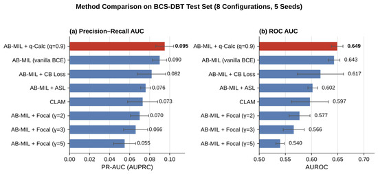
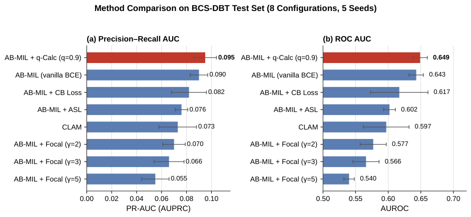
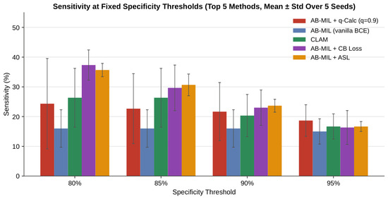
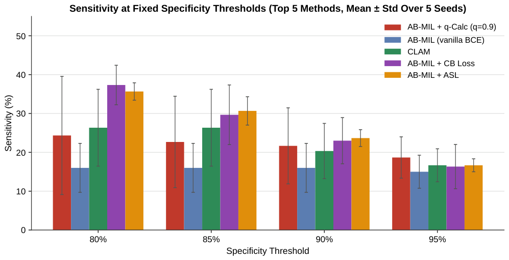
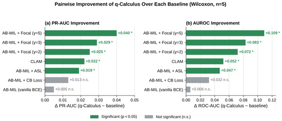
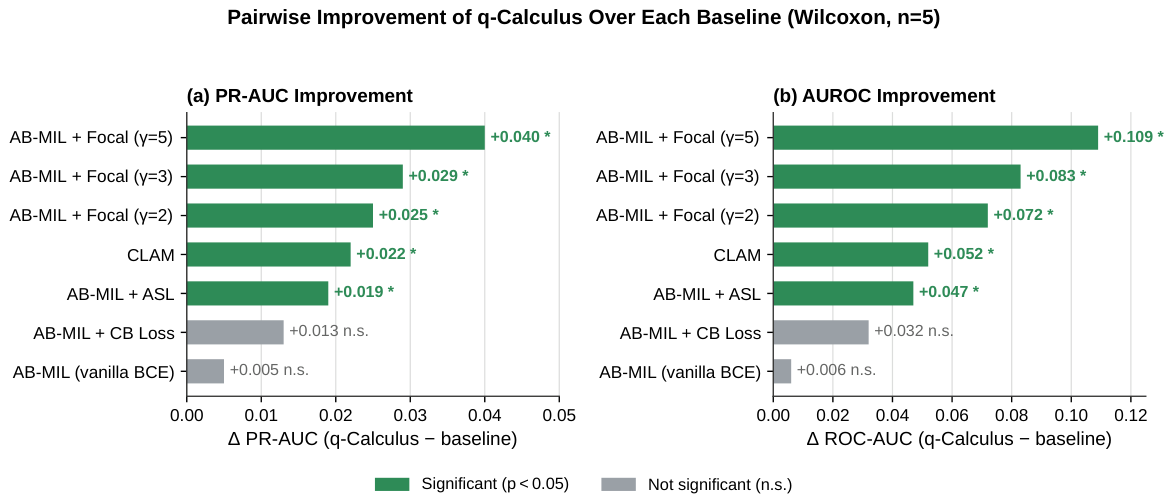
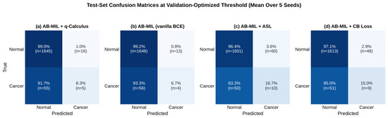
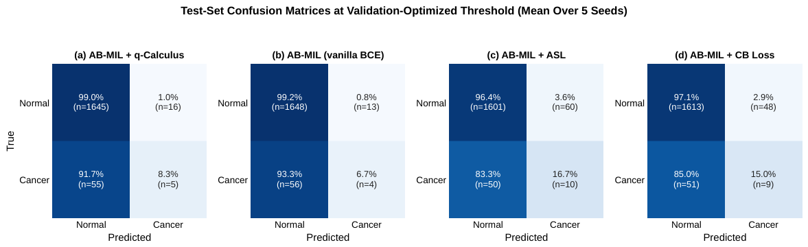
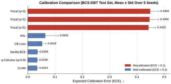
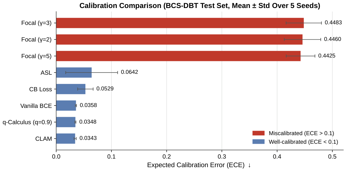
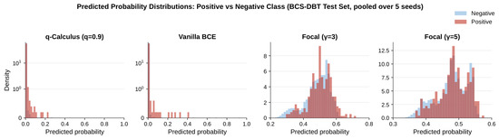
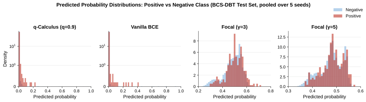

Disclaimer/Publisher’s Note: The statements, opinions and data contained in all publications are solely those of the individual author(s) and contributor(s) and not of MDPI and/or the editor(s). MDPI and/or the editor(s) disclaim responsibility for any injury to people or property resulting from any ideas, methods, instructions or products referred to in the content. |
© 2026 by the authors. Licensee MDPI, Basel, Switzerland. This article is an open access article distributed under the terms and conditions of the Creative Commons Attribution (CC BY) license.