Functional Kolmogorov-Arnold Network: A Hilbert-Space Perspective on Spatial Representation Learning for Medical Image Segmentation

Abstract

Medical image segmentation requires spatial transformations that remain effective across heterogeneous image statistics and boundary conditions. We introduce FunKAN, a KAN-inspired operator that acts directly on spatial feature maps: analytical Hermite basis maps are evaluated on an input-conditioned deformed grid, scored against learned channel-wise templates, mixed by a softmax over modes, and aggregated across channels. A Hilbert-space functional approximation result motivates the function-space viewpoint, while the exact finite FunKAN operator is treated separately and is not claimed to inherit a universal-approximation theorem. We embed FunKAN in a U-shaped architecture (U-FunKAN) and evaluate it under the validation-only selection protocol on BUSI, GlaS, and CVC-ClinicDB. The frozen model is tested once per seed after three-seed training. U-FunKAN improves mean test IoU over a same-protocol U-Net by 6.35 percentage points on BUSI and 1.85 points on CVC-ClinicDB, while GlaS performance is comparable, with U-FunKAN 0.50 points lower. U-FunKAN uses fewer parameters than the retrained U-Net (15.95 M vs. 31.03 M) but is substantially slower in measured GPU latency, so we do not claim universal computational efficiency. The results support dataset-dependent gains from functional spatial parameterization rather than uniform dominance.

1. Introduction

Medical imaging is central to screening, diagnosis, treatment planning, and longitudinal monitoring. In this pipeline, segmentation is a core dense prediction task because it provides pixel-level delineation of anatomical structures and pathological regions for downstream quantitative analysis [1]. The task remains difficult in modalities such as ultrasound, histopathology, and endoscopy, where boundaries are often ambiguous, appearance varies across patients and acquisition settings, and clinically relevant structures span multiple scales.

Deep learning is now the dominant approach to medical image segmentation. Encoder-decoder architectures, especially U-Net [2], established a good template that combines multi-scale aggregation and precise localization using skip connections. Later attention, denser feature fusion, and longer-range modeling, including Attention U-Net [3], U-Net++ [4], nnU-Net [5], and U-Mamba [6] were added. These models perform well in practice, but rely on standard nonlinear blocks with only indirect links to approximation-theoretic transformations.

Kolmogorov-Arnold networks (KANs) [7] have recently attracted attention as an alternative to conventional multilayer perceptrons. Motivated by the Kolmogorov-Arnold representation theorem [8], KANs replace fixed pointwise activations with learnable univariate functions. This yields a more structured view of nonlinear approximation. The idea has led to a growing ecosystem of variants that differ mainly in how these functions are parameterized, including spline-based, polynomial, radial-basis, and orthogonal-basis constructions [7,9,10,11]. KAN-style ideas have also begun to appear in medical imaging, including U-KAN [12] and MedKAN [13]. Related work has also explored convolutional KAN constructions [14].

These developments [7] provide learnable scalar nonlinearities, but most KAN formulations are primarily defined for vectors of scalar features. Visual adaptations therefore often use flattening, tokenization, patchwise processing, or KAN layers embedded within otherwise conventional architectures; the precise choice varies by method. Such adaptations do not directly formulate each feature-map channel as an element of a function space. They consequently provide a less natural parameterization for dense prediction, where spatial topology and coherent pixel-level outputs must be maintained. Existing KAN variants provide learnable scalar nonlinearities, but a principled KAN-inspired parameterization that operates directly on spatial feature maps as functions, while retaining their spatial organization and providing an explicit finite mode-count parameter, remains insufficiently explored for dense medical image prediction.

We address this gap with the functional Kolmogorov-Arnold network (FunKAN). Each feature-map channel is treated as a function sampled on a spatial grid. A Hilbert-space and Riesz-representation perspective motivates the general use of function-space measurements, while the actual FunKAN block uses a more specific finite factorization: analytical Hermite basis maps are evaluated on an input-conditioned deformed grid, correlated with learned channel-wise spatial templates, mixed across Hermite modes by a softmax, and finally mixed across channels. FunKAN therefore retains intermediate feature maps without flattening while providing a differentiable function-based parameterization. We implement this idea in a U-shaped framework, yielding U-FunKAN.

We evaluate the approach on three medical image segmentation benchmarks spanning ultrasound, histopathology, and colonoscopy. The paper uses a validation-only architecture and loss search, freezes the selected configuration before test access, and retrains a classic U-Net under the same split, loss, optimizer, checkpoint, and seed protocol. The resulting test behavior is dataset dependent: U-FunKAN yields a large gain on BUSI, a moderate gain on CVC-ClinicDB, and near parity with U-Net on the official GlaS test split. GPU profiling additionally shows that the FunKAN operator has a nontrivial wall-clock cost despite a smaller parameter count and lower THOP-reported MAC count. We therefore frame the contribution as a functional spatial parameterization with selective empirical gains, not as universal accuracy or speed dominance.

Our contributions are:

• We propose FunKAN, a KAN-inspired block that transforms spatial feature maps using Hermite basis evaluation, input-conditioned coordinate offsets, learned spatial templates, softmax mode mixing, and channel mixing without flattening the feature field.
• We instantiate FunKAN in U-FunKAN and provide an implementation-level description that distinguishes the exact finite operator from its Hilbert-space motivation.
• We evaluate U-FunKAN on three 2D segmentation benchmarks under the stated validation-only model-selection protocol, with the final architecture frozen before test evaluation and three independent final seeds.
• We provide validation-only ablations of BN, width, Hermite order, deformation, backbone grid, depth, and BCE weight, together with a same-protocol U-Net control and batch-size-dependent GPU latency profiling.
• We state the approximation-theoretic motivation and the conditional truncation, discretization, interpolation, and deformation bounds without claiming that the exact softmax-factorized FunKAN block inherits universality from the motivating theorem.

2. Materials and Methods

2.1. Problem Formulation

We consider dense prediction over medical images, with a primary focus on semantic segmentation. Let $I\in {\mathbb{R}}^{H\times W\times C}$ denote an input image and let $Y\in {\{0,1\}}^{H\times W}$ denote the corresponding pixel-level target mask. The goal is to learn a mapping

$${\mathcal{F}}_{\theta }:{\mathbb{R}}^{H\times W\times C}\to {[0,1]}^{H\times W}$$

that predicts spatially coherent segmentations across heterogeneous imaging conditions.

Parameterizing nonlinear transformations on intermediate feature maps is challenging in standard segmentation architectures, especially when spatial structure must be preserved. Standard segmentation architectures [2,5] typically treat nonlinearities as pointwise activation functions composed with spatial operators such as convolutions or attention. In contrast, recent Kolmogorov-Arnold networks (KANs) [7] replace fixed nonlinearities with learnable functions, but they are primarily defined on vectors of scalar inputs. This is undesirable for dense prediction tasks where geometric structure must be preserved. We therefore design the method around a simple goal: keep intermediate representations as spatial feature maps throughout the network while using a more structured nonlinear transformation than standard pointwise activations. To this end, we introduce the functional Kolmogorov-Arnold network (FunKAN), a KAN-style layer that operates directly on feature maps instead of flattened vectors. Each channel is treated as a function defined over the image grid, and the layer transforms these channels through input-conditioned basis evaluation, template scoring, nonlinear mode mixing, and channel mixing.

2.2. Theoretical Motivation

Intermediate feature-map channels may be viewed as elements of a Hilbert space such as $H=L_2(\Omega )$. Functional neural-network approximation results [15] motivate architectures that process functions through continuous linear functionals followed by scalar nonlinear mixing. If $\mathit{\ell }\in H^{\ast }$ is a continuous linear functional, the Riesz representation theorem gives a unique $u\in H$ such that $\mathit{\ell }\left(x\right)={\langle x,u\rangle }_H$. This supplies a useful function-space viewpoint for spatial feature maps.

The following theorem is used only as architectural motivation. It is not an implementation prescription and does not imply that the exact FunKAN parameterization below is a universal approximator.

Theorem 1 

(Functional neural-network approximation on compact sets). Let $K\subset H^n$ be compact and let $f\in C\left(K\right)$. Assume an activation $\sigma :\mathbb{R}\to \mathbb{R}$ satisfying the density conditions in [15]. For every $\epsilon >0$ there exist $m\in \mathbb{N}$, continuous linear functionals ${\mathit{\ell }}_{ji}\in H^{\ast }$, and scalars $a_j,b_j$ such that

$$g(x_1,\dots ,x_n)={\displaystyle \sum _{j=1}^m}{a}_j\sigma \left({\displaystyle \sum _{i=1}^n}{\mathit{\ell }}_{ji}\left(x_i\right)+b_j\right)$$

satisfies

$$\underset{(x_1,\dots ,x_n)\in K}{\sup }|f(x_1,\dots ,x_n)-g(x_1,\dots ,x_n)|<\epsilon .$$

The symbols ${\mathit{\ell }}_{ji}$ denote abstract scalar-valued functionals, and their Riesz representers are denoted by $u_{ji}$. Appendix A gives the precise scope of Theorem 1, a Hermite truncation bound for Riesz representers, and a theory-to-implementation mapping. In particular, the appendix explicitly identifies an implementation gap: the softmax-factorized FunKAN block is inspired by the functional construction but is not algebraically identical to it.

2.3. Functional Operator Layer

We now describe the exact finite-dimensional operator used in the experiments (see Figure 1). This notation intentionally differs from the abstract functionals ${\mathit{\ell }}_{ji}$ in Theorem 1.

Let the input to layer l be ${\chi }_{l-1}\in {\mathbb{R}}^{n\times h\times w}$, and let $q=(q_x,q_y)$ index the reference grid. A residual CNN $D_l$ predicts channel-wise offsets $({\Delta }_l^x,{\Delta }_l^y)=D_l\left({\chi }_{l-1}\right)$. For Hermite mode $k\in \{0,\dots ,r-1\}$, the separable basis map is

$$B_{l,ik}(q;{\chi }_{l-1})={\psi }_k\left(q_x+{\Delta }_{l,i}^x(q;{\chi }_{l-1})\right){\psi }_k\left(q_y+{\Delta }_{l,i}^y(q;{\chi }_{l-1})\right).$$

(1)

For each input channel i, the layer contains a learned spatial template $T_{l,i}\in {\mathbb{R}}^{h\times w}$. In the released source code this parameter is named phi; we use T in the paper to avoid overloading the symbol for a linear functional. The discrete mode score and normalized mode weight are

$$s_{l,ik}=\sum _q{B}_{l,ik}(q;{\chi }_{l-1})T_{l,i}\left(q\right),{\alpha }_{l,ik}={\displaystyle \frac{\exp \left(s_{l,ik}\right)}{{\sum }_{k^{\prime }=0}^{r-1}\exp \left(s_{l,i{k}^{\prime }}\right)}}.$$

(2)

The reconstructed channel is

$$z_{l,i}\left(q\right)={\displaystyle \sum _{k=0}^{r-1}}{\alpha }_{l,ik}{B}_{l,ik}(q;{\chi }_{l-1}),$$

(3)

and the m output channels are obtained by the $1\times 1$ convolution

$${\chi }_{l,j}\left(q\right)=b_{l,j}+{\displaystyle \sum _{i=1}^n}{W}_{l,ji}{z}_{l,i}\left(q\right),j=1,\dots ,m.$$

(4)

Thus $T_l\in {\mathbb{R}}^{n\times h\times w}$, the basis tensor has shape $B_l\in {\mathbb{R}}^{n\times r\times h\times w}$ for each sample, and $W_l\in {\mathbb{R}}^{m\times n\times 1\times 1}$. The index i always denotes an input channel, j an output channel, and k a basis mode.

This exact factorization also clarifies the theoretical scope. The weights ${\alpha }_{l,ik}$ lie in a probability simplex, so the per-channel reconstruction is a convex combination of basis maps before the signed $1\times 1$ channel mixing. Therefore, density of an unconstrained Hermite span does not directly imply density of the implemented softmax-factorized family. Appendix A makes this distinction explicit and does not claim a universal-approximation theorem for Equations (1)–(4).

2.4. Spatial Grid Deformation

The offset network (see Figure 2) changes the coordinates at which the analytical Hermite functions are evaluated. It does not bilinearly resample the input feature map. Specifically, the model uses $q+{\Delta }_{l,i}(q;{\chi }_{l-1})$ in Equation (1). This makes the basis input adaptive while preserving the spatial tensor layout.

Following pre-activation residual design principles [16], the offset field is produced by a small residual CNN. A diffeomorphic coordinate-change interpretation is possible only conditionally: for each input, the map $q\mapsto q+\Delta \left(q\right)$ would need to be invertible with controlled Jacobian. These conditions are not enforced during standard training. Appendix A therefore treats diffeomorphism as a sufficient theoretical condition rather than a property guaranteed by the implementation, and instead gives a local perturbation bound for bounded offsets. Bilinear interpolation appears separately when the latent feature map is resized to the selected backbone grid; it is not part of the learned offset operation.

2.5. Model Architecture: U-FunKAN

We implement FunKAN within a U-shaped encoder-decoder segmentation architecture, denoted U-FunKAN. An overview is shown in Figure 3. The encoder progressively increases feature dimensionality while reducing spatial resolution. FunKAN backbone then transforms the latent feature maps. The decoder restores spatial resolution through upsampling and skip connections.

The architecture is selected on the BUSI development split and then frozen before any test evaluation. The selected configuration is:

1.

Embedding: a $3\times 3$ convolution projects the RGB input to 64 channels.

2.

Lifting: four residual encoder blocks use output widths $128\to 160\to 256\to 256$, with each stage reducing spatial resolution by a factor of two using a strided $3\times 3$ convolution.

3.

Backbone: three FunKAN blocks operate at latent width 256. Each block uses $r=10$ diagonal separable Hermite modes, a $24\times 24$ backbone grid, full anchored input-conditioned deformation, and no batch normalization.

4.

Projection: the decoder mirrors the selected filter list, reducing channels $256\to 256\to 160\to 128\to 64$ while restoring spatial resolution and fusing encoder skip features.

5.

Restoration: a final $1\times 1$ convolution maps the decoded features to one output logit channel.

The frozen U-FunKAN contains 15.95 million trainable parameters. For $256\times 256$ inputs, the native encoder output after four downsamplings is $16\times 16$; for GlaS at $512\times 512$ it is $32\times 32$. In both cases the latent feature field is bilinearly resized to the selected $24\times 24$ backbone grid before the FunKAN stack and is resized back for the decoder. This deterministic resizing is distinct from the learned coordinate offsets, which modify the locations at which Hermite basis functions are evaluated.

For segmentation, the network is trained with a weighted sum of binary cross-entropy and soft Dice loss:

$${\mathcal{L}}_{\mathrm{segm}}={\lambda }_{\mathrm{BCE}}\mathrm{BCEWithLogits}(y,z)+\left(1-{\displaystyle \frac{2{\sum }_p\sigma \left(z_p\right)y_p+1}{{\sum }_p\sigma \left(z_p\right)+{\sum }_p{y}_p+1}}\right),$$

(5)

where z denotes output logits, y the binary reference mask, p indexes pixels, and the Dice smoothing constant is 1.0. Validation macro IoU selects ${\lambda }_{\mathrm{BCE}}=0.5$ over the search $\{0,0.05,0.1,0.2,0.5\}$, which is frozen with the architecture before final test evaluation.

The implemented two-dimensional dictionary uses diagonal products ${\psi }_k\left(q_x\right){\psi }_k\left(q_y\right)$ rather than the complete tensor-product family ${\psi }_a\left(q_x\right){\psi }_b\left(q_y\right)$. The order r is therefore an empirical mode-count–cost parameter, not a monotone approximation guarantee for the exact softmax-factorized implementation. The validation search compares $r\in \{2,4,6,8,10\}$ and selects $r=10$.

We evaluate U-FunKAN on three publicly available 2D medical image segmentation benchmarks spanning breast ultrasound, gland histopathology, and colonoscopy polyp segmentation.

2.6. Datasets

2.6.1. BUSI Dataset

The BUSI dataset [17] is used for binary breast-lesion segmentation. We use the 647 benign and malignant source ultrasound images and exclude the normal class. Some source images have more than one lesion-mask file; before splitting, all masks associated with the same source image are merged by a pixelwise logical OR so that one source image constitutes exactly one sample. The provided split preserves the held-out set after removing source-image duplication, resulting in 130 test images. The remaining 517 development images are divided with split seed 42 into 413 training and 104 validation images, stratified by benign/malignant class. BUSI images are resized to $256\times 256$.

2.6.2. GlaS Dataset

The GlaS dataset [18] is used for gland segmentation in H&E histopathology. The primary protocol follows the official 85-image training/80-image test partition. Only the official training portion is split further: with seed 42, 68 images are used for parameter fitting and 17 for validation; the official 80-image test set remains unchanged. Images are resized to $512\times 512$. Exact identifiers are distributed in data_lists/glas/train.csv, val.csv, and test.csv.

2.6.3. CVC-ClinicDB Dataset

The CVC-ClinicDB dataset [19] contains 612 colonoscopy images with pixel-level polyp annotations. We retain the 123-image held-out evaluation list and split the remaining 489 development images with seed 42 into 391 training and 98 validation images. CVC-ClinicDB images are resized to $256\times 256$.

2.6.4. Selection and Test Protocol

All the stated selection decisions are made from training and validation data only. The BUSI development pipeline is pre-specified as: BN versus no-BN stability, channel widths, Hermite order, deformation design, backbone grid, FunKAN depth, and BCE coefficient. The BN comparison uses seeds 50, 100, 150, 200, and 250 and is ranked by mean validation macro IoU. The remaining sequential stages use seed 100 and carry the winner of each stage into the next stage. This sequential design is a model-selection procedure, so values from different stages should not be interpreted as isolated causal effects.

After the last validation stage, the complete state is serialized and frozen (see

Table 1. Reproducibility-critical settings for the segmentation experiments. Values that are selected by validation are frozen before test evaluation.

Setting	Protocol
Optimizer	Adam; LR ${10}^{-4}$; $\beta =(0.9,0.999)$; $\epsilon ={10}^{-8}$; weight decay 0; AMSGrad off
Schedule/stopping	No LR scheduler; no early stopping; maximum 1000 epochs
Precision/determinism	FP32; deterministic Lightning execution; cuDNN benchmark off
Effective batch	8 examples/optimizer step; micro-batch/accumulation specified in text; validation 1; test 1
Loss	Dice loss (smooth 1.0) $+{\lambda }_{\mathrm{BCE}}$ BCEWithLogits; selected ${\lambda }_{\mathrm{BCE}}=0.5$ from $\{0,0.05,0.1,0.2,0.5\}$
Final training seeds	50, 100, 150
BN stability seeds	50, 100, 150, 200, 250
Primary checkpoint rule	maximum validation image-macro IoU
Prediction threshold	sigmoid probability $>0.5$
Metric aggregation	IoU/F1 per image → arithmetic macro mean per seed → mean ± sample SD across seeds
Empty prediction + empty target	IoU $=1$, F1 $=1$
Test-time augmentation/post-processing	none/none
DataLoader	0 workers; pin memory on; training shuffle on; validation/test shuffle off; drop-last off

): filters $[64,128,160,256,256]$, $r=10$, full anchored deformation, no BN, $24\times 24$ backbone grid, depth 3, and ${\lambda }_{\mathrm{BCE}}=0.5$. Final U-FunKAN benchmarking uses seeds 50, 100, and 150. For each seed, the checkpoint with maximum validation image-macro IoU is selected before test access and is evaluated on the corresponding test set exactly once. The primary controlled baseline is a classic U-Net retrained with the same data lists, loss, optimizer, epoch budget, validation checkpoint rule, seeds, prediction threshold, and metric aggregation. Literature-reported models remain useful context but are not pooled into the primary controlled table because their split and training protocols differ. Instead, the provided numerical results are generated from the validation-only pipeline described above. The supplied scripts create a test-access gate and record a frozen architecture hash before final evaluation; test execution is enabled only after all required U-FunKAN and U-Net train/validation runs are complete. Exact split files, hashes, selected checkpoints, and run metadata are distributed with the Supplementary Materials Package.

Dataset licenses and usage conditions are summarized in the reproducibility and data-availability subsection below.

2.7. Implementation Details

All experiments are specified for Python 3.12, PyTorch 2.5.0+cu118, Lightning 2.5.1, AlbumentationsX 2.0.9, OpenCV 4.11.0.86, and NumPy 2.1.2. Segmentation training is performed in 32-bit precision on an NVIDIA RTX A6000 (see Table 1). The complete pinned package environment is supplied in requirements/requirements.txt; the runtime-capture utility additionally records the GPU model, driver, CUDA and cuDNN versions, package versions, and repository commit for each experiment host.

Models are trained from scratch with Adam [20]: learning rate ${10}^{-4}$, ${\beta }_1=0.9$, ${\beta }_2=0.999$, $\epsilon ={10}^{-8}$, weight decay 0, and AMSGrad disabled. The runs use no learning-rate scheduler and no early stopping; the maximum training length is 1000 epochs. The effective training batch is 8 examples per optimizer step. To fit the selected model and the controlled U-Net on the available GPUs without changing the optimizer-step batch, gradient accumulation is used where needed: U-FunKAN uses micro-batch 8/8/2 with accumulation 1/1/4 on BUSI/CVC/GlaS, respectively; U-Net uses micro-batch 4/4/1 with accumulation 2/2/8. Validation and test batch size is 1. Both final architectures are BN-free, so these micro-batch changes do not introduce batch-statistics differences. Data loaders use zero worker subprocesses, training shuffling only, pinned host memory, and no dropped final batch. Lightning deterministic mode is enabled, cuDNN benchmarking is disabled, and all Python/NumPy/PyTorch worker seeds are initialized through seed_everything(..., workers=True).

2.7.1. Preprocessing and Augmentation

Training augmentation is applied only after the split has been fixed. For all segmentation datasets, vertical flip, horizontal flip, random 90° rotation, and transposition are each independently enabled with probability 0.5. An additional arbitrary-angle rotation is enabled with probability 0.5 and samples uniformly from [−90°, 90°]; image interpolation is bilinear, mask interpolation is nearest-neighbor, the border mode is constant with zero image/mask fill, and border cropping is disabled. Validation and test data receive no stochastic augmentation. All segmentation images are resized to the dataset-specific resolution in

Table 2. Data partitions used in the experiments. Validation samples are drawn only from the corresponding development/training partition; no test image is used for the model, checkpoint, or hyperparameter selection.

Dataset	Train	Validation	Test	Model Input
BUSI	413	104	130	$256\times 256$
GlaS	68	17	80	$512\times 512$
CVC-ClinicDB	391	98	123	$256\times 256$

, normalized per image with the pinned AlbumentationsX min–max normalization, and converted to tensors. No test-time augmentation or morphological post-processing is used.

2.7.2. Checkpointing, Hyperparameter Selection, and Initialization

Segmentation checkpoints are written every epoch, but only the checkpoint with maximum validation macro IoU is retained for final evaluation (save_top_k=1); the last checkpoint is stored only for diagnostics. No checkpoint is selected from training loss or test performance. The final validation-selected state is filters $[64,128,160,256,256]$, $r=10$, full anchored deformation, no BN, grid $24\times 24$, depth 3, and ${\lambda }_{\mathrm{BCE}}=0.5$. FunKAN spatial templates $T_{\mathit{\ell },i}$ are initialized orthogonally; convolutional layers otherwise use their PyTorch-defined initialization. The controlled U-Net baseline uses the classic double-convolution encoder–decoder with feature widths $[64,128,256,512]$ and the same Dice+BCE objective with ${\lambda }_{\mathrm{BCE}}=0.5$. The exact frozen architecture hash, split hashes, selected checkpoint, and seed are recorded for every final run.

2.7.3. Segmentation Metrics

For each test image, probabilities are obtained with a sigmoid and thresholded at 0.5. IoU and F1 are then computed from that image’s binary contingency table,

$$\mathrm{IoU}={\displaystyle \frac{TP}{TP+FP+FN}},F_1={\displaystyle \frac{2TP}{2TP+FP+FN}}.$$

(6)

If both prediction and reference are empty, both metrics are defined as 1.0. Metrics are first averaged arithmetically over images for each seed. Table-level values then report the mean and sample standard deviation across the three final seeds (50, 100, 150).

2.7.4. Computational Profiling

Parameter counts are measured directly from the frozen models. THOP output is reported as GMACs rather than being labeled GFLOPs without a conversion convention. GPU latency is measured on an NVIDIA RTX A6000 in FP32 at batch sizes 1, 2, 4, 8, and 16, using 50 warm-up iterations followed by 200 synchronized timed iterations per batch size. No mixed precision or TF32 setting is introduced for the profiling run.

2.8. Reproducibility, Data Availability, and Ethical Considerations

All datasets used in this study are publicly available research datasets. The study did not involve new data acquisition, intervention on human participants, or intervention on animals. Accordingly, no new institutional ethical approval was required for the computational experiments reported here. To support reproducibility, the codebase, configuration files, and dataset split definitions are intended for release with the manuscript.

Licenses and Usage of External Assets

The BUSI dataset [17], GlaS dataset [18], and CVC-ClinicDB dataset [19] are used for academic research under the access and usage conditions specified by their respective providers. PyTorch and PyTorch Lightning are used under their BSD-style licenses. All datasets and software were used in accordance with their respective terms.

3. Results

3.1. Primary Same-Protocol Segmentation Comparison

Table 3. Same-protocol test comparison. Each model is trained independently with seeds 50, 100, and 150; the best checkpoint for each seed is selected only by validation macro IoU and evaluated on the test set once. Values are mean ± sample SD across the three seeds. Bold indicates the better result for each dataset and metric. ↑ indicates that higher values are better.

Method	BUSI		GlaS Official Test		CVC-ClinicDB
	IoU↑	F1↑	IoU↑	F1↑	IoU↑	F1↑
U-Net (retrained)	$65.21\pm 1.27$	$73.73\pm 1.21$	$\mathbf{79.47}\pm \mathbf{1.36}$	$\mathbf{87.94}\pm \mathbf{0.97}$	$86.67\pm 0.69$	$91.92\pm 0.44$
U-FunKAN (ours)	$\mathbf{71.55}\pm \mathbf{1.32}$	$\mathbf{80.26}\pm \mathbf{1.14}$	$78.97\pm 1.41$	$87.36\pm 1.08$	$\mathbf{88.52}\pm \mathbf{0.58}$	$\mathbf{93.16}\pm \mathbf{0.34}$
Paired mean difference (ours − U-Net), pp	$+6.35$	$+6.53$	$-0.50$	$-0.58$	$+1.85$	$+1.25$

reports the held-out test results. The primary comparison includes only U-FunKAN and the classic U-Net retrained under the same split, loss, optimizer, checkpoint-selection, seed, threshold, and metric-aggregation protocol. Values are mean ± sample standard deviation across seeds 50, 100, and 150; IoU and F1 are first computed per image and macro-averaged within each seed.

U-FunKAN yields the clearest improvement on BUSI: mean IoU increases by 6.35 percentage points and mean F1 by 6.53 points relative to the same-protocol U-Net. The gain on CVC-ClinicDB is smaller but positive for all three seeds, with mean improvements of 1.85 IoU points and 1.25 F1 points. On the official GlaS test split, the two models are close and U-Net is slightly higher on average by 0.50 IoU points and 0.58 F1 points. We therefore do not claim that U-FunKAN universally dominates U-Net across datasets. The GlaS result is especially useful as a check against post-test tuning: although U-FunKAN had higher validation IoU during final training, no architecture or hyperparameter was changed after observing the official test result.

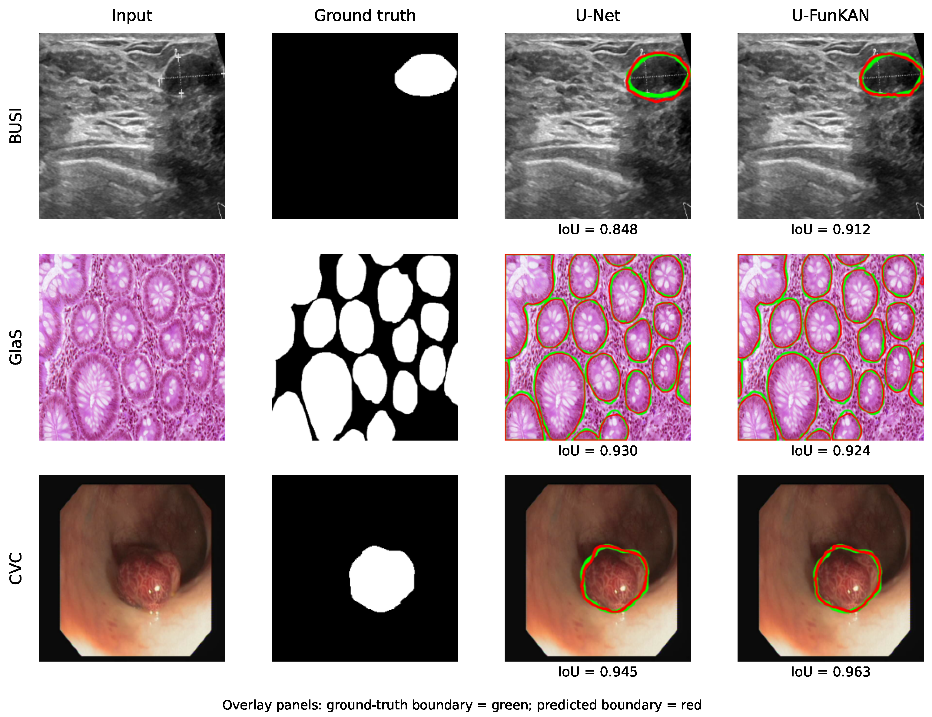
To complement the aggregate test metrics with a visual assessment of segmentation quality, Figure 4 shows one illustrative example from each test dataset. To avoid selecting cases solely on the basis of a favorable U-FunKAN outcome, we use a model-symmetric deterministic selection rule. For each dataset, we first restrict the candidates to the upper quartile according to the mean per-image IoU of U-Net and U-FunKAN, and then select the case whose U-FunKAN-minus-U-Net IoU difference is closest to the corresponding dataset-level mean difference reported in Table 3. Thus, the examples provide visually clear segmentations while preserving the qualitative pattern of the complete test-set comparison: a clear U-FunKAN advantage on BUSI, near parity with a slight U-Net advantage on GlaS, and a smaller U-FunKAN advantage on CVC-ClinicDB. In the prediction panels, green contours indicate the ground-truth boundary and red contours indicate the predicted boundary.

The comparisons against U-NeXt, U-KAN, KM-UNet, and other literature models are not used because those values were produced under heterogeneous split and training protocols. These methods remain discussed as related work, but Table 3 is deliberately restricted to the model that was retrained under the same controlled protocol.

3.2. Validation-Only Model Selection and Ablation

The selection history is summarized in

Table 4. First part of the BUSI validation-only selection. BN values are mean ± sample SD across five seeds; width and Hermite-order rows are independent seed-100 candidates within their respective sequential stages. Bold entries indicate the winner carried forward. No test metric was available to the selection code.

Stage	Candidate	Trainable Params (M)	Validation IoU (%)	Validation F1 (%)
BN stability	BN	3.637	$72.63\pm 0.39$	$81.23\pm 0.45$
	No BN	3.635	$\mathbf{74.93}\pm \mathbf{0.92}$	$\mathbf{83.10}\pm \mathbf{0.67}$
Width	$[16,32,64,128,128]$	3.635	74.86	83.07
	$[32,64,96,128,128]$	4.133	75.50	83.40
	$[\mathbf{64},\mathbf{128},\mathbf{160},\mathbf{256},\mathbf{256}]$	15.701	75.59	83.66
	$[128,256,320,512,512]$	62.391	72.78	81.32
Hermite order	$r=2$	15.701	74.58	82.47
	$r=4$	15.701	74.90	83.11
	$r=6$	15.701	75.17	83.37
	$r=8$	15.701	75.39	83.56
	$\mathbf{r}=\mathbf{10}$	15.701	75.60	83.74

and 

Table 5. Second part of the BUSI validation-only sequential selection (seed 100). Bold entries indicate the winner passed to the next stage. The final BCE winner completes the frozen model.

Stage	Candidate	Trainable Params (M)	Validation IoU (%)	Validation F1 (%)
Deformation	Fixed basis grid	6.851	68.78	77.56
	Offset only	15.701	74.38	82.55
	Full anchored deformation	15.701	75.39	83.51
Backbone grid	$8\times 8$	15.553	74.87	83.06
	$16\times 16$	15.701	74.93	83.27
	$\mathbf{24}\times \mathbf{24}$	15.946	75.43	83.47
	$32\times 32$	16.290	74.67	82.78
	$48\times 48$	17.273	73.87	82.58
FunKAN depth	1	9.620	74.31	82.91
	2	12.783	74.94	83.13
	3	15.946	75.41	83.64
${\lambda }_{\mathrm{BCE}}$	0	15.946	69.43	78.70
	0.05	15.946	74.20	82.50
	0.10	15.946	75.11	83.18
	0.20	15.946	75.58	83.74
	$\mathbf{0}.\mathbf{50}$	15.946	75.97	83.96

. The first BN decision uses five pre-specified seeds; all later stages use seed 100 and pass only the validation winner to the next stage. Accordingly, the tables document the actual selection path and should not be read as a factorial causal decomposition.

The five-seed BN experiment selects the BN-free configuration: its mean validation IoU is 74.93% versus 72.63% with BN, and no-BN is higher for all five paired seeds. The mean paired no-BN minus BN improvement is 2.29 percentage points (sample SD 0.90). The subsequent width stage selects filters $[64,128,160,256,256]$; the much wider 62.4M-parameter candidate performs worse, so larger width is not monotonically beneficial. The Hermite-order stage increases gradually over the tested range and selects $r=10$.

Full anchored deformation is selected over the fixed-grid and offset-only variants. The grid experiment peaks at $24\times 24$ and then degrades at $32\times 32$ and $48\times 48$, which argues against interpreting finer discretization as automatically better. Three FunKAN blocks outperform one and two in the sequential depth stage. Finally, the BCE ablation directly addresses the coefficient: pure Dice is substantially worse, the value 0.1 is competitive but not optimal, and the validation rule selects ${\lambda }_{\mathrm{BCE}}=0.5$. This coefficient is frozen before the final test stage.

3.3. Batch-Size-Dependent GPU Profiling

Table 6. GPU computational profile at $256\times 256$ input resolution. Latency is median milliseconds per image; throughput is based on median batch latency. THOP values are reported as GMACs. Bold indicates the better result for each computational metric (lower for parameters, GMACs, latency, and peak memory; higher for throughput).

Method	Params (M)	THOP GMACs	B1	B2	B4	B8	B16	Throughput B8 (img/s)	Peak Mem. B16 (MB)
U-Net	31.03	54.61	5.60	5.30	4.87	4.64	3.77	215.30	9596.6
U-FunKAN	15.95	43.31	70.51	35.75	19.38	18.80	20.44	53.19	3207.9

reports the batch-size scaling on an NVIDIA RTX A6000 in FP32. Each latency point uses 50 warm-up iterations and 200 synchronized timed iterations. THOP reports multiply-accumulate counts (MACs), not FLOPs; moreover, custom operators can be under-counted by generic profilers, so the measured wall-clock timings are the primary runtime evidence.

U-FunKAN has about half as many trainable parameters as the retrained U-Net and a lower THOP-reported MAC count, but it is much slower in wall-clock inference. At batch 1, its median latency is 70.51 ms per image versus 5.60 ms for U-Net; at batch 8, the corresponding values are 18.80 and 4.64 ms per image. U-FunKAN also uses less measured peak memory in this profile. The discrepancy between generic MAC counting and latency reflects the cost and hardware utilization of the custom basis/deformation operations.

4. Discussion

Under the same-protocol comparison, the model provides the strongest result on BUSI, where it improves mean test IoU by 6.35 percentage points and F1 by 6.53 points over U-Net. On CVC-ClinicDB the gain is more modest but positive for all three seeds. On the official GlaS test set, however, U-FunKAN and U-Net are close and U-Net is slightly higher on average. This pattern supports a dataset-dependent inductive-bias interpretation rather than a claim of universal dominance.

The provided selection results also make the architectural evidence more precise. Removing BN improves BUSI validation IoU across all five paired seeds. The sequential search selects an intermediate width rather than the largest candidate, $r=10$ within the tested Hermite orders, full anchored deformation, a $24\times 24$ grid, three FunKAN blocks, and ${\lambda }_{\mathrm{BCE}}=0.5$. Because these stages are sequential rather than factorial, their numbers identify the selected path but do not isolate independent causal contributions. In particular, the present experiments do not establish that Hermite functions are universally better than Fourier, radial-basis, spline, or other fixed dictionaries. Hermite functions should therefore be understood as the basis used by the current implementation, supported here by an order ablation and by the function-space analysis, not as an empirically proven optimal basis family.

The computational results claim that U-FunKAN has fewer trainable parameters and lower THOP-reported MACs than the retrained U-Net, but substantially higher measured GPU latency. Generic operation counters do not fully characterize the cost of the custom basis/deformation path, and wall-clock performance depends on kernel structure and hardware utilization.

Within the validation-only selection pipeline, architecture and loss decisions were based exclusively on training and validation data. The final configuration was frozen before the reported test evaluation, and no architecture or hyperparameter was changed after observing the test results. This provides a more realistic estimate of generalization.

Improved overlap metrics can correspond to more accurate delineation of lesions or polyps, but IoU and F1 are not clinical outcomes. The public-benchmark experiments do not establish diagnostic benefit, safety, calibration, fairness, robustness to distribution shift, or cross-institutional generalization. U-FunKAN should therefore be viewed as a representation-learning research model rather than an autonomous clinical system.

Limitations

First, the empirical study is limited to three public 2D segmentation datasets and one same-protocol controlled baseline. The classic U-Net is controlled for data lists, optimization, checkpointing, seeds, thresholding, and metric aggregation, but it is not parameter matched to U-FunKAN (31.03 M versus 15.95 M trainable parameters); the comparison therefore isolates the complete trained architectures rather than a capacity-matched FunKAN substitution. Additional architectures, capacity-matched controls, and external datasets would be needed to determine how broadly the observed BUSI/CVC gains transfer.

Second, the model uses a fixed Hermite family and a diagonal two-dimensional dictionary. We did not perform a matched Fourier/RBF/spline basis-family experiment in this work, so no claim of Hermite-basis superiority is made. Determining which basis family is best for a given modality remains open.

Third, the functional approximation theorem is architectural motivation rather than a universality theorem for the exact FunKAN block. The implementation uses learned template–basis correlations, input-conditioned offsets, softmax-constrained mode weights, and diagonal Hermite products. Appendix A therefore separates the abstract Riesz/Hermite construction from the finite operator and treats the remaining implementation gap explicitly.

Fourth, the learned deformation is not constrained to be globally invertible. Diffeomorphic interpretations are therefore conditional, and the appendix provides only the corresponding local bounded-offset perturbation statement for the implemented basis evaluation.

Fifth, the current implementation has high GPU latency relative to U-Net despite its smaller parameter count. Optimized kernels, basis caching, mixed precision, or alternative factorization strategies may change that trade-off, but they were not evaluated here.

5. Conclusions

We introduced FunKAN, a KAN-inspired spatial functional parameterization, and U-FunKAN, its U-shaped segmentation realization. The exact implementation evaluates Hermite basis maps on input-conditioned deformed coordinates, scores them with learned spatial templates, applies softmax mode mixing, and then mixes channels. A Hilbert-space approximation perspective motivates the design, while the theory explicitly avoids transferring universality claims to the finite softmax-factorized operator.

Under a validation-only protocol, the frozen U-FunKAN improves mean test IoU over a same-protocol U-Net by 6.35 percentage points on BUSI and 1.85 points on CVC-ClinicDB, while the official GlaS test result is comparable and slightly favors U-Net by 0.50 points. U-FunKAN uses fewer trainable parameters but is substantially slower in measured GPU inference. The resulting conclusion is therefore: functional spatial parameterization can provide meaningful gains on some medical segmentation datasets, but the magnitude of the gain and the computational trade-off are dataset- and implementation-dependent.

References

- Kadhim, Y.A.; Khan, M.U.; Mishra, A. Deep learning-based Computer-Aided Diagnosis (CAD): Applications for Medical Image Datasets. Sensors 2022, 22, 8999. [Google Scholar] [CrossRef] [Scilit] [PubMed]
- Ronneberger, O.; Fischer, P.; Brox, T. U-Net: Convolutional Networks for Biomedical Image Segmentation. In Proceedings of the International Conference on Medical Image Computing and Computer-Assisted Intervention; Springer: Berlin/Heidelberg, Germany, 2015; pp. 234–241. [Google Scholar]
- Oktay, O.; Schlemper, J.; Folgoc, L.L.; Lee, M.; Heinrich, M.; Misawa, K.; Mori, K.; McDonagh, S.; Hammerla, N.Y.; Kainz, B.; et al. Attention U-Net: Learning Where to Look for the Pancreas. arXiv 2018, arXiv:1804.03999. [Google Scholar]
- Zhou, Z.; Rahman Siddiquee, M.M.; Tajbakhsh, N.; Liang, J. UNet++: A Nested U-Net Architecture for Medical Image Segmentation. In Proceedings of the International Workshop on Deep Learning in Medical Image Analysis; Springer: Berlin/Heidelberg, Germany, 2018; pp. 3–11. [Google Scholar]
- Isensee, F.; Jaeger, P.F.; Kohl, S.A.; Petersen, J.; Maier-Hein, K.H. nnU-Net: A Self-configuring Method for Deep Learning-based Biomedical Image Segmentation. Nat. Methods 2021, 18, 203–211. [Google Scholar] [CrossRef] [Scilit] [PubMed]
- Ma, J.; Li, F.; Wang, B. U-Mamba: Enhancing Long-range Dependency for Biomedical Image Segmentation. arXiv 2024, arXiv:2401.04722. [Google Scholar]
- Liu, Z.; Wang, Y.; Vaidya, S.; Ruehle, F.; Halverson, J.; Soljačić, M.; Hou, T.Y.; Tegmark, M. KAN: Kolmogorov-Arnold Networks. arXiv 2024, arXiv:2404.19756. [Google Scholar]
- Kolmogorov, A.N. On the Representations of Continuous Functions of Many Variables by Superposition of Continuous Functions of One Variable and Addition. Dokl. Akad. Nauk USSR 1957, 114, 953–956. [Google Scholar]
- Li, Z. Kolmogorov-Arnold Networks are Radial Basis Function Networks. arXiv 2024, arXiv:2405.06721. [Google Scholar]
- Seydi, S.T. Exploring the Potential of Polynomial Basis Functions in Kolmogorov-Arnold Networks: A Comparative Study of Different Groups of Polynomials. arXiv 2024, arXiv:2406.02583. [Google Scholar]
- Sidharth, S.; Keerthana, A.; Anas, K. Chebyshev Polynomial-based Kolmogorov–Arnold Networks: An Efficient Architecture for Nonlinear Function Approximation. arXiv 2024, arXiv:2405.07200. [Google Scholar]
- Li, C.; Liu, X.; Li, W.; Wang, C.; Liu, H.; Liu, Y.; Chen, Z.; Yuan, Y. U-KAN Makes Strong Backbone for Medical Image Segmentation and Generation. Proc. AAAI Conf. Artif. Intell. 2025, 39, 4652–4660. [Google Scholar] [CrossRef] [Scilit]
- Yang, Z.; Zhang, J.; Luo, X.; Lu, Z.; Shen, L. MedKAN: An Advanced Kolmogorov-Arnold Network for Medical Image Classification. arXiv 2025, arXiv:2502.18416. [Google Scholar]
- Drokin, I. Kolmogorov-Arnold Convolutions: Design Principles and Empirical Studies. arXiv 2024, arXiv:2407.01092. [Google Scholar]
- Stinchcombe, M.B. Neural Network Approximation of Continuous Functionals and Continuous Functions on Compactifications. Neural Netw. 1999, 12, 467–477. [Google Scholar] [CrossRef] [Scilit] [PubMed]
- Duta, I.C.; Liu, L.; Zhu, F.; Shao, L. Improved Residual Networks for Image and Video Recognition. In Proceedings of the 2020 25th International Conference on Pattern Recognition (ICPR); IEEE: New York, NY, USA, 2021; pp. 9415–9422. [Google Scholar]
- Al-Dhabyani, W.; Gomaa, M.; Khaled, H.; Fahmy, A. Dataset of Breast Ultrasound Images. Data Brief 2020, 28, 104863. [Google Scholar] [CrossRef] [Scilit] [PubMed]
- Sirinukunwattana, K.; Pluim, J.P.W.; Chen, H.; Qi, X.; Heng, P.A.; Guo, Y.B.; Wang, L.Y.; Matuszewski, B.J.; Bruni, E.; Sanchez, U.; et al. Gland segmentation in colon histology images: The GlaS challenge contest. Med. Image Anal. 2017, 35, 489–502. [Google Scholar] [CrossRef] [Scilit] [PubMed]
- Bernal, J.; Sánchez, F.J.; Fernández-Esparrach, G.; Gil, D.; Rodríguez, C.; Vilariño, F. WM-DOVA Maps for Accurate Polyp Highlighting in Colonoscopy: Validation vs. Saliency Maps from Physicians. Comput. Med. Imaging Graph. 2015, 43, 99–111. [Google Scholar] [CrossRef] [Scilit] [PubMed]
- Kingma, D.P.; Ba, J. Adam: A Method for Stochastic Optimization. In Proceedings of the 3rd International Conference on Learning Representations (ICLR), San Diego, CA, USA, 7–9 May 2015. [Google Scholar]
- Davis, P.J.; Rabinowitz, P. Methods of Numerical Integration; Academic Press: Cambridge, MA, USA, 1975. [Google Scholar]
- Brenner, S.C.; Scott, R.L. The Mathematical Theory of Finite Element Methods, 3rd ed.; Springer: Berlin/Heidelberg, Germany, 2008. [Google Scholar]
Figure 1.
Scheme of the proposed finite FunKAN factorization. For each input channel , the offset network predicts input-conditioned coordinate shifts and analytical Hermite functions are evaluated at the shifted coordinates, producing basis maps . Each basis map is scored against a learned channel-wise spatial template (the parameter named phi in the released code); a softmax across modes produces weights . The weighted basis maps form , and a convolution mixes channels to produce . The output index j enters only at the final channel-mixing step.
Figure 2.
Scheme of the spatial grid deformation module. A residual CNN predicts unconstrained coordinate offsets that are added to the reference coordinates before analytical basis evaluation. The input feature map itself is not resampled. Because the offsets are unconstrained, global invertibility or positivity of the deformation Jacobian is not guaranteed by the implemented model.
Figure 3.
Overview of the frozen U-FunKAN segmentation architecture. Four residual encoder blocks produce the latent field, which is deterministically resized to the selected backbone grid, processed by three FunKAN blocks, resized back, and decoded with encoder skip features.
Figure 4.
Qualitative segmentation examples from the held-out BUSI, official GlaS, and CVC-ClinicDB test sets. Columns show the input image, ground-truth mask, and contour-overlay visualizations for the same-protocol U-Net and U-FunKAN predictions. In the overlay panels, the ground-truth boundary is shown in green and the predicted boundary in red. Predictions are obtained from the validation-selected seed-100 checkpoints using the fixed probability threshold of 0.5. For each dataset, the displayed case is selected from the upper quartile of joint model quality, measured by the mean IoU of U-Net and U-FunKAN, and is the case whose U-FunKAN-minus-U-Net IoU difference is closest to the dataset-level mean difference in