


Abstract
Anomaly detection systems deployed in critical applications require not only high accuracy but also reliable uncertainty quantification and coverage guarantees. This paper is an empirical study—rather than a contribution of new conformal-prediction machinery—of class-conditional (Mondrian) conformal prediction for anomaly detection under extreme class imbalance, characterizing where standard conformal prediction fails and how class-conditional calibration restores valid coverage. Class-conditional conformal prediction constructs prediction sets that, under exchangeability, contain the true label with user-specified confidence (e.g., 90%), enabling systems to abstain on uncertain predictions. Unlike standard conformal prediction that fails catastrophically under extreme imbalance—achieving only 52.94% anomaly coverage at a 1:345 imbalance ratio—class-conditional calibration maintains 90.59% anomaly coverage by computing quantiles separately for each class. We apply the standard softmax-based nonconformity score within each class, ensuring valid coverage for both normal and anomalous instances with coverage gaps ranging from 0.50% to 5.18% depending on dataset characteristics. Extensive experiments on three real-world datasets (Microsoft Azure KPI, Yahoo, NAB) demonstrate that the method achieves empirical coverage within 0.06–0.33% of theoretical targets at confidence levels ; on the most imbalanced benchmark (Microsoft Azure KPI at a 1:345 ratio and ), this corresponds to a 37.65 percentage point improvement in anomaly coverage over standard conformal prediction. We restate finite-sample coverage bounds and exchangeability conditions in the binary anomaly detection setting and validate them empirically through Monte Carlo simulation. Multi-model evaluation across XGBoost, Random Forest, and Neural Networks demonstrates the model-agnostic property of the framework, while also identifying conditions (poor base-classifier discrimination, small minority calibration sets) under which coverage may be marginally violated. Comparison with alternative uncertainty quantification methods (isotonic probability calibration, Monte Carlo dropout) shows that only conformal prediction provides formal guarantees while maintaining 90.59% anomaly coverage versus 76.47% and 84.71% for alternatives. The abstention mechanism identifies 34–66% of predictions as uncertain at high confidence levels (99%), enabling safety-critical systems to defer difficult cases to human experts while preserving baseline discrimination (ROC-AUC unchanged).
1. Introduction
Anomaly detection is a fundamental problem in machine learning with critical applications across diverse domains, including fraud detection [1], medical diagnosis [2], industrial monitoring [3], and cybersecurity [4]. While modern machine learning models have achieved impressive performance on anomaly detection tasks, a significant challenge remains: how can we trust the predictions of these models, especially in high-stakes scenarios where errors can have severe consequences? Traditional anomaly detection methods focus primarily on maximizing detection accuracy through metrics such as F1-score, precision, and recall [5,6]. However, in safety-critical applications, knowing when the model is uncertain is equally important as achieving high accuracy. A fraud detection system that confidently misclassifies a legitimate transaction as fraudulent can cause significant financial loss and customer dissatisfaction. Similarly, a medical diagnostic system that fails to express uncertainty about a borderline case may lead to inappropriate treatment decisions. The challenge becomes even more pronounced in the presence of extreme class imbalance, a characteristic feature of most real-world anomaly detection problems [7,8]. In typical scenarios, anomalous instances constitute less than 1% of the total data, with imbalance ratios reaching 1:100 or higher. Under such conditions, standard machine learning models tend to exhibit bias toward the majority class [9], and their probability estimates become poorly calibrated [10], making uncertainty quantification unreliable. Conformal prediction (CP) has emerged as a principled framework for uncertainty quantification that provides distribution-free coverage guarantees [11,12]. Unlike traditional uncertainty estimation methods that rely on distributional assumptions or asymptotic properties, conformal prediction constructs prediction sets that provably contain the true label with a user-specified probability. The key advantage of CP is its model-agnostic nature: it can be applied to any base classifier without requiring modifications to the underlying model architecture [13]. However, standard (marginal) conformal prediction faces significant challenges when applied to imbalanced data. The marginal coverage guarantee ensures that the true label is covered across the entire test distribution, but this does not guarantee adequate coverage for minority classes [14,15]. In anomaly detection scenarios with extreme imbalance, standard CP may achieve the desired overall coverage while systematically failing to cover anomalous instances—precisely the cases that are most critical to identify correctly. In this paper, we conduct a focused empirical study of how a known remedy for this failure—class-conditional (Mondrian) conformal prediction [12,14]—behaves in the binary anomaly detection regime under extreme imbalance, where prior class-conditional CP work has provided limited evaluation. By computing separate nonconformity quantiles for each class, valid coverage guarantees can be obtained for both normal and anomalous instances, regardless of the imbalance ratio. We emphasize at the outset that the contribution of this paper is empirical and methodologically applied rather than a new conformal-prediction algorithm: we do not propose novel CP machinery, but instead characterize the operational regime in which an existing remedy (class-conditional/Mondrian CP) becomes essential, document its failure modes, and quantify its finite-sample behavior under extreme imbalance. Accordingly, the quantitative headline figures reported below (for example, the 37.65 percentage-point coverage improvement and the 0.06–0.33% coverage gaps) should be read as properties of specific datasets and settings, not as general guarantees of the method.
Our main contributions are:
- Empirical Characterization Under Extreme Imbalance: We provide an empirical characterization of class-conditional CP in the binary anomaly detection regime at imbalance ratios up to a 1:345, where prior CC-CP evaluations focused on balanced or moderately imbalanced multi-class settings. On the Microsoft Azure KPI dataset specifically (1:345 imbalance, ), we document a 37.65 percentage-point improvement in anomaly coverage over standard conformal prediction; the magnitude is dataset- and -dependent, and the corresponding figures for all datasets and confidence levels are reported in Section 5.2.
- Restatement of Coverage Guarantees in the Binary Setting: We restate class-conditional coverage and finite-sample bounds for the binary anomaly detection case, making them directly usable by practitioners, and we validate the finite-sample bound empirically via Monte Carlo simulation.
- Comprehensive Baseline Comparisons: We compare against standard conformal prediction (showing its failure under extreme imbalance), evaluate across multiple base models (XGBoost version 2.1.4, and Random Forest and Neural Networks (multi-layer perceptron) implemented in scikit-learn version 1.5.2), and contrast with alternative uncertainty quantification methods (isotonic probability calibration in scikit-learn version 1.5.2, and a Monte Carlo dropout ensemble surrogate built on XGBoost version 2.1.4).
- Practical Abstention Mechanism: The framework naturally identifies uncertain predictions through ambiguous prediction sets, enabling systems to defer difficult cases to human experts. This mechanism is crucial for safety-critical deployments.
- Extensive Empirical Validation: We demonstrate on three real-world benchmark datasets that this approach achieves empirical coverage within 0.06–0.33% of theoretical targets at strict confidence levels () while preserving baseline discrimination (ROC-AUC unchanged). (Code and notebook are publicly available at https://github.com/BashairAlthani/Conformal_Prediction_Project (accessed on 2 June 2026).)
- The remainder of this paper is organized as follows. Section 2 reviews related work on anomaly detection, uncertainty quantification, and conformal prediction. Section 3 presents the class-conditional conformal prediction framework as applied here, including formal theoretical guarantees. Section 4 describes the experimental setup and datasets. Section 5 presents comprehensive experimental results including comparisons with standard CP and alternative UQ methods. Section 6 discusses the practical implications and limitations. Finally, Section 7 concludes the paper and outlines future research directions.
2. Related Work
2.1. Anomaly Detection Under Extreme Class Imbalance
Modern anomaly detection systems confront fundamental challenges arising from severe class imbalance, where normal instances vastly outnumber anomalies—often by ratios exceeding 1000:1 in real-world applications. While deep learning approaches have achieved notable success in capturing complex patterns, their performance degrades substantially under extreme imbalance, primarily due to biased optimization toward majority classes. Recent theoretical work by [7] provides an exact solution through replica theory, revealing that optimal training imbalance differs substantially from balanced configurations, with non-trivial dependencies on intrinsic imbalance and noise levels. Their analysis distinguishes between intrinsic, training, and test imbalance—a taxonomy critical for understanding when standard methods fail. Contemporary approaches attempt to mitigate imbalance through data-level interventions (synthetic oversampling, undersampling) or algorithm-level modifications (cost-sensitive learning, focal loss). However, these techniques introduce their own pathologies. Synthetic minority oversampling techniques such as SMOTE [16] may introduce noise by interpolating between sparse minority examples, while undersampling discards potentially informative majority-class patterns; recent applied work in healthcare-fraud detection illustrates these trade-offs in practice [17]. More concerning, algorithmic solutions that adjust decision boundaries or loss functions provide no statistical guarantees on false positive rates or coverage for minority-class predictions—a critical gap when deploying models in safety-critical or high-stakes domains [8]. The lack of principled uncertainty quantification under imbalance remains a persistent limitation across state-of-the-art anomaly detectors, including isolation forests, autoencoders, and transformer-based approaches [6].
2.2. Uncertainty Quantification and Model Calibration in Deep Learning
The machine learning community has increasingly recognized that predictive accuracy alone provides insufficient guarantees for reliable decision-making. Model calibration—ensuring that predicted probabilities align with true outcome frequencies—has emerged as a complementary objective. Ref. [10] demonstrated that modern neural networks, despite high accuracy, produce poorly calibrated confidence estimates, often exhibiting overconfidence on incorrect predictions. This miscalibration problem intensifies under class imbalance, where majority-class priors dominate probability estimates. Recent uncertainty quantification methods employ diverse strategies: Bayesian neural networks capture epistemic uncertainty through weight distributions, ensemble approaches aggregate predictions across multiple models, and evidential deep learning quantifies uncertainty via higher-order probability distributions [18]. Yet these techniques face computational constraints and often lack finite-sample guarantees. Ref. [19] provides a comprehensive survey revealing that while Bayesian approximations (e.g., Monte Carlo dropout, variational inference) offer theoretical elegance, they require careful hyperparameter tuning and may fail to provide reliable uncertainty estimates in distribution-shift scenarios. Furthermore, post hoc probability calibration methods such as temperature scaling, Platt scaling, and isotonic regression adjust outputs but do not fundamentally address the underlying miscalibration mechanisms, particularly when applied to imbalanced or minority-class predictions [20].
2.3. Conformal Prediction: Theory and Applications to Anomaly Detection
Conformal prediction (CP), rooted in the foundational work of [12], offers a distribution-free framework for constructing prediction sets with finite-sample validity guarantees. Under the exchangeability assumption—weaker than i.i.d.—split conformal prediction provides marginal coverage: for a user-specified miscoverage rate , the prediction set contains the true label with probability of at least . This guarantee holds regardless of the underlying model, making CP particularly attractive for wrapping around black-box deep learning systems. Recent theoretical extensions by [15] relax exchangeability to accommodate covariate shift and non-stationary data through weighted conformal methods, broadening applicability to real-world scenarios with temporal or distributional drift. Applications to anomaly detection have gained momentum. Ref. [21] introduces context-aware prediction-powered conformal online anomaly detection (C-PP-COAD), addressing calibration data scarcity by strategically integrating synthetic data while maintaining false discovery rate (FDR) control. Ref. [22] develops ECAD, a distribution-free ensemble conformal anomaly detection method for spatio-temporal data with missing observations. In aviation safety, ref. [23] demonstrates practical utility for identifying unstable flight approaches and trajectory anomalies with explicit uncertainty quantification. However, these methods predominantly target marginal coverage guarantees—ensuring that across all test points, coverage holds on average—which proves insufficient when specific subpopulations (e.g., rare anomaly types) require individual coverage assurances. Standard CP under severe imbalance allocates calibration budget uniformly, resulting in prediction sets that either overcover common classes (low utility) or undercover minorities (safety violations).
2.4. Class-Conditional and Imbalance-Aware Conformal Prediction
Recognizing the limitations of marginal coverage, prior work has developed class-conditional guarantees: ensuring that for each class y, the prediction set contains y with probability when y is the true label. The canonical approach is classwise (Mondrian) CP, introduced by [12], which performs separate conformal calibration per class. Classwise CP becomes impractical when calibration data is limited relative to the number of classes; ref. [14] addresses this through clustered conformal prediction, which groups similar classes based on score distributions and performs calibration at the cluster level, achieving tighter prediction sets than classwise methods in low-data regimes with hundreds of classes. Building on this foundation, ref. [24] proposes Rank-Calibrated Class-conditional CP (RC3P), which employs augmented label rank calibration to selectively iterate class-wise thresholding only for classes with small top-k error. They report a 26.25% average reduction in prediction set sizes while maintaining class-wise coverage; we note, however, that this figure was obtained on multi-class image-classification benchmarks (CIFAR-100, ImageNet-scale and similar) with hundreds to a thousand classes and per-class calibration sets that, while smaller than in balanced settings, remain far larger than the ∼20 minority samples encountered in our binary extreme-imbalance regime—so the reported set-size reduction should not be assumed to transfer directly to our setting. Ref. [25] introduces self-calibrating conformal prediction that combines Venn–Abers calibration with conformal inference to provide both calibrated point predictions and prediction intervals with conditional validity, but their development and evaluation target regression and probability calibration rather than binary detection under extreme class imbalance. These advances represent significant progress for balanced or moderately imbalanced classification tasks. However, their evaluation focuses on ImageNet-scale datasets (1000 classes) with relatively balanced calibration sets, leaving practical questions open: How does extreme imbalance (e.g., <1% anomaly prevalence) affect coverage when only a handful of minority calibration samples are available? How tight are finite-sample bounds in this regime?
2.5. Research Gap and Contributions
Despite substantial progress in both anomaly detection under imbalance and class-conditional conformal prediction, prior CC-CP evaluations have not focused on the binary anomaly-detection regime under extreme imbalance, where minority calibration sets may contain only ∼20 samples. The gap is concrete rather than rhetorical: the clustered conformal prediction of [14] was designed for and evaluated on many-class problems (hundreds of classes) where the difficulty is sharing calibration data across classes, and it does not examine a binary 1:345 regime with a ∼21-sample minority set; the RC3P method of [24] targets top-k set-size efficiency on balanced-to-moderately imbalanced image benchmarks and reports class-wise coverage in that setting, but does not test whether its finite-sample corrections hold when one class has ∼20 calibration points; and the self-calibrating CP of [25] establishes conditional validity for calibrated regression/probability outputs rather than binary minority-class coverage under <1% prevalence. Standard conformal approaches, meanwhile, optimize for marginal coverage and systematically undercover rare anomalies to maintain overall calibration. What none of these works demonstrate—and what we therefore study here—is the behavior of finite-sample corrections, the practical magnitude of class-coverage disparities, and the consequences of base-classifier miscalibration when class-conditional CP is pushed into the binary, extreme-imbalance regime.
This work addresses these gaps with a focused empirical study of class-conditional (Mondrian) conformal prediction in binary anomaly detection under extreme imbalance. We adopt the standard softmax-based nonconformity score within each class and quantify coverage, finite-sample effects, abstention behavior, and base-model sensitivity at imbalance ratios of 1:25, 1:33, and 1:345. The contribution is empirical and methodological-applied rather than novel CP machinery: we identify the operational regime where class-conditional CP is essential, document failure modes (including a marginal coverage violation under a poorly calibrated base classifier), and provide practitioner-facing guidance.
3. Methodology
In this section, we present the class-conditional conformal prediction framework as applied to binary anomaly detection. We start by explaining the basic problem setup, then describe how standard conformal prediction works, present the class-conditional procedure, restate the relevant theoretical guarantees, and finally explain how the system can abstain on uncertain predictions.
3.1. Problem Setup and Preliminaries
We consider a binary classification problem where we need to distinguish between two types of instances: normal instances (labeled as ) representing regular, expected behavior, and anomalies (labeled as ) representing unusual, unexpected behavior. Let represent the space of all possible inputs (such as sensor readings or transaction features) and represent the two possible labels. We have a dataset containing n examples, where each example consists of an input and its corresponding label . Our framework builds upon a base classifier—in our case, XGBoost (version 2.1.4) —that has already been trained to predict anomalies. This classifier takes an input x and produces two probability estimates: representing the probability that x is normal, and representing the probability that x is an anomaly. These probabilities sum to 1, meaning the classifier must choose between the two possibilities. A critical characteristic of anomaly detection is extreme class imbalance: anomalies are rare events. In plain terms, the probability of encountering an anomaly is much smaller than the probability of encountering a normal instance. In our experiments, anomalies represent as little as 0.29% of the data, creating a 1:345 imbalance ratio where for every anomaly, there are 345 normal instances. This extreme imbalance presents practical challenges for providing reliable coverage guarantees, which motivates the class-conditional approach.
3.2. Standard Split Conformal Prediction
Conformal prediction addresses a fundamental question: How confident should we be in a model’s prediction? Rather than just outputting a single predicted label, conformal prediction produces a prediction set —a set of possible labels that is guaranteed to contain the true label with a user-specified probability (e.g., 90% or 95%). The key insight is to use past prediction errors on a calibration dataset to determine appropriate confidence thresholds for future predictions, providing mathematical guarantees about reliability. The process begins by dividing the available data into two independent parts: a training set used to train the base classifier, and a calibration set used to measure the classifier’s uncertainty and compute appropriate thresholds. This separation is crucial because it ensures the calibration is unbiased—we test the model on data it has not seen during training. For each example in the calibration set, we compute a nonconformity score that measures how “strange” or “unexpected” the prediction was. Specifically, for a calibration point with true label , the score is calculated as , which represents one minus the probability the model assigned to the true class. This score is small (near 0) when the model was confident and correct—for example, if the model assigned 95% probability to the true class, the score is only 0.05. Conversely, the score is large (near 1) when the model was uncertain or wrong—if the model assigned only 30% probability to the true class, the score is 0.70. Given a desired confidence level specified by significance level (for example, corresponds to 90% confidence), we compute a threshold from the calibration scores. This threshold is chosen so that of the calibration scores fall below it, with a small adjustment factor to account for finite sample size and ensure the guarantee holds for new test data. For a new test point, we construct a prediction set by including all labels whose nonconformity scores would be “typical”—that is, below the threshold. In plain terms, we include label y in the prediction set if the model assigns it enough probability that its nonconformity score would not be unusually high. The fundamental guarantee of conformal prediction is remarkably simple yet powerful: with probability of at least (e.g., 90%), the true label will be included in the prediction set. This guarantee holds regardless of the data distribution, model architecture, or problem domain—it only requires that the data points are exchangeable (roughly, independent and identically distributed).
3.3. Class-Conditional Conformal Prediction
While standard conformal prediction provides overall coverage guarantees, it has a critical limitation in imbalanced settings. Consider a scenario where 99% of instances are normal and only 1% are anomalies. A method could achieve 90% overall coverage by covering 91% of normal instances (which are abundant in the data) but covering only 0% of anomalies (which are rare). This satisfies the mathematical guarantee but fails catastrophically for the minority class—precisely the anomalies we care most about detecting correctly. This happens because the single threshold is dominated by the majority class: since most calibration points are normal instances, the threshold becomes tuned to normal instances, leaving anomalies undercovered. The class-conditional (Mondrian) remedy [12] is conceptually simple: compute separate thresholds for each class. Instead of one threshold that tries to work for all instances, we create specialized thresholds—one calibrated specifically for normal instances and one calibrated specifically for anomalies—ensuring both classes receive proper coverage regardless of how imbalanced the data is. This approach recognizes that normal instances and anomalies may have fundamentally different uncertainty patterns, and each deserves its own calibration. Figure 1 summarizes the end-to-end class-conditional conformal prediction pipeline, from a trained base classifier and a labeled calibration set through class-stratified threshold estimation to the construction of a prediction set (and possible abstention) for a new test instance. We present the corresponding algorithm as instantiated in this work in Algorithm 1. The algorithm proceeds in four steps. First, we stratify the calibration set by separating it into class-specific subsets: one containing only normal instances and one containing only anomalies. This allows us to examine each class independently. Second, for each class, we compute the standard softmax-based nonconformity score [12] restricted to that class’s calibration subset—for normal instances, the score is one minus the probability assigned to “normal”; for anomalies, the score is one minus the probability assigned to “anomaly.” Third, we calculate separate quantile thresholds for each class using only the scores from that class’s calibration subset. This produces (the threshold for normal instances) and (the threshold for anomalies). Finally, when making predictions for a new test point, we compare its scores against the class-specific thresholds—we check the “normal” score against the normal threshold and the “anomaly” score against the anomaly threshold—and include in the prediction set any class whose score falls below its respective threshold.
| Algorithm 1 Class-Conditional Conformal Prediction for Binary Anomaly Detection |
| Input: Trained classifier f, calibration set , significance level (e.g., 0.10 for 90% coverage) |
| Output: Prediction set function with class-conditional coverage guarantees |
| 1: Step 1: Stratify Calibration Set by Class |
| 2: // Separate calibration data into class-specific subsets |
| 3: {all calibration examples with label 0 (normal)} |
| 4: {all calibration examples with label 1 (anomaly)} |
| 5: |
| 6: Step 2: Compute Class-Specific Nonconformity Scores |
| 7: // For each class, measure how well the model predicted instances of that class |
| 8: For each normal instance in : |
| 9: // Score = 1 minus probability of being normal |
| 10: For each anomaly in : |
| 11: // Score = 1 minus probability of being anomaly |
| 12: |
| 13: Step 3: Compute Class-Specific Thresholds |
| 14: // Calculate separate quantile thresholds for each class |
| 15: -quantile of // Threshold for normal class |
| 16: -quantile of // Threshold for anomaly class |
| 17: // Each threshold is calibrated using only that class’s data |
| 18: |
| 19: Step 4: Construct Prediction Set for New Test Instance |
| 20: // For test point x, compare its scores against class-specific thresholds |
| 21: // Initialize empty prediction set |
| 22: If : // Normal score below normal threshold? |
| 23: Add class 0 (normal) to |
| 24: If : // Anomaly score below anomaly threshold? |
| 25: Add class 1 (anomaly) to |
| 26: |
| 27: return Prediction set containing 0, 1, both, or neither class |
Figure 1.
Class-conditional (Mondrian) conformal prediction pipeline for binary anomaly detection. The calibration set is stratified by class; a separate nonconformity-score quantile (, ) is estimated for each class; and a new test point is admitted to the prediction set for every class whose score falls below the corresponding class threshold, yielding a confident singleton ( or ) or an abstention () routed to a human reviewer.
The intuition is straightforward. By calibrating separate thresholds using only data from each class, we ensure that the coverage guarantee applies independently to each class. When we set (requesting 90% confidence), the class-conditional approach guarantees that at least 90% of normal instances will have their true label in the prediction set and at least 90% of anomalies will have their true label in the prediction set. These guarantees hold simultaneously, regardless of how imbalanced the data is. This is exactly what we need for reliable anomaly detection under extreme class imbalance—we cannot sacrifice coverage on the rare but critical anomaly class just because anomalies are outnumbered.
3.4. Theoretical Guarantees
We now restate the relevant theoretical guarantees for the class-conditional (Mondrian) conformal procedure in the binary setting, including coverage guarantees, finite-sample bounds, and exchangeability conditions. The results below are direct consequences of standard Mondrian CP theory [12,14], restated here in a form that is directly applicable to binary anomaly detection.
Theorem 1
(Class-Conditional Coverage Guarantee, restated from [12]). Let be exchangeable random variables taking values in . Let be any classifier. For each class , let be the indices of calibration points belonging to class k, and let be the size of this set. For significance level , define class-specific nonconformity scores:
Define class-specific quantiles with finite-sample correction:
Then, the prediction set
satisfies, for each class :
Proof.
The argument is the standard split conformal coverage argument applied within each class (Mondrian CP [12]). Fix a class and condition on the event . Step 1 (Conditional exchangeability of scores). Let and define for . By the exchangeability of , the conditional joint distribution of the scores given the multiset of class labels and their counts is invariant under permutations of the indices. In particular, conditional on and on , the augmented score vector is exchangeable. Step 2 (Rank-based coverage). By exchangeability, the rank of among the scores is uniformly distributed on when ties have probability zero (and the inequality ≤ is preserved by a standard tie-breaking argument otherwise). Hence,
where denotes the j-th order statistic of the calibration scores in class k. Step 3 (Quantile identification). The quantile defined in the theorem equals by construction (using the standard “higher” interpolation convention on the empirical CDF of the calibration scores). Step 4 (Set membership). By definition of , the event coincides with . Combining Steps 2–4 yields , as claimed. □
Remark 1
(Conditional versus marginal coverage in ). The coverage bound in Theorem 1 is conditional on the realized per-class calibration count , not marginal over its distribution. This is explicit in Step 1 of the proof, where we condition on and on before invoking the rank argument; the resulting rank of is uniform on for the observed , so the guarantee holds for the calibration set actually drawn rather than only on average across hypothetical re-draws of the class sizes. The distinction is operationally important under extreme imbalance: when is as small as ≈21 (Microsoft), the achievable quantile levels form a coarse grid , so for a given α the realized coverage is pinned to the nearest attainable grid point above for that specific calibration draw. Reporting coverage conditionally on (as we do) is therefore the honest characterization for a practitioner who must deploy with one fixed, small minority calibration set; the seed-to-seed variation we report in Section 5 then captures the residual effect of re-drawing that small set. A fully marginal statement—averaging the guarantee over the random class counts—would additionally smooth over this grid effect and would understate the conservativeness that any single small- deployment actually experiences.
Theorem 2
(Finite-Sample Overcoverage Bound). Under the conditions of Theorem 1, and assuming the calibration scores within class k are continuously distributed (so ties occur with probability zero), the empirical coverage for class k is bounded:
Proof.
The lower bound follows from Theorem 1. For the upper bound, by the same rank argument with no ties, for each . Choosing gives an exact coverage probability of at most . □
Remark 2
(Interpretation of Finite-Sample Effects). Theorem 2 explains the overcoverage phenomenon observed in our experiments. For small calibration sets (e.g., Microsoft anomaly class with ), the maximum overcoverage at the strict-coverage end of the bound is approximately . As the calibration set grows, this bound decreases, approaching the target coverage. The overcoverage is conservative (coverage ≥ target), which is desirable for safety-critical applications, but it can be substantial when both α is large and is small (cf. Section 5).
Definition 1
(Exchangeability). A sequence of random variables is exchangeable if for any permutation π of :
In practice, exchangeability holds when data points are independent and identically distributed (i.i.d.), but is more general—it allows for certain forms of dependence.
Remark 3
(Exchangeability in Time-Series Anomaly Detection). The benchmarks studied here (Azure KPI, Yahoo, NAB) are time series, and temporal dependence can in principle violate exchangeability. We address this at three levels. When approximate exchangeability is supported. Three conditions act together: temporal ordering, in that training and calibration data precede the test set; feature engineering, in that the 25 rolling-window and lag features absorb autocorrelation into the feature space so that residual nonconformity scores are closer to i.i.d.; and empirical stability, in that seed-to-seed standard deviations in Section 5 remain below across five independent calibration draws, which provides indirect evidence that temporal dependence does not appreciably destabilize the quantile estimates. When exchangeability may be violated. Severe concept drift, strong autocorrelation in the residual nonconformity scores, and strong seasonal structure can each break the assumption; ref. [15] shows that conformal prediction degrades gracefully under mild violations, bounding the coverage loss by the total-variation distance between the test and calibration marginals. Chronological-split caveat. A strictly chronological train → calibration → test split is the gold standard for deployment simulation; we instead use stratified random splits because the Microsoft anomalies cluster temporally, so a chronological split yields a near-empty anomaly calibration set and makes class-conditional quantile estimation infeasible. Practitioners with larger labeled anomaly pools should prefer chronological splits, and formal residual diagnostics (Ljung–Box tests on the nonconformity-score sequences, block-permutation validation, and ADWIN-based drift detection) are identified as priority future experiments.
These theoretical results establish that the class-conditional framework, as instantiated here, provides:
- Valid coverage for each class independently, regardless of imbalance ratio;
- Finite-sample guarantees that hold for any sample size, with tighter bounds as grows;
- Distribution-free validity under only the mild exchangeability assumption.
3.5. Prediction Set Interpretation and Abstention
Unlike traditional classifiers that output a single label, conformal prediction outputs a set of plausible labels. This set can have different sizes, each conveying different information about the model’s certainty. A prediction set containing only one class (either or ) indicates a confident prediction —the system is sure enough to make a definitive call. A prediction set containing both classes () indicates uncertainty—the system cannot confidently distinguish between normal and anomaly at the required confidence level and should abstain from making a decision. An empty prediction set (∅) is rare and indicates extreme uncertainty, typically handled by defaulting to the class with the highest probability. The ability to abstain from uncertain predictions is particularly valuable in safety-critical anomaly detection. When the prediction set contains both classes, this signals that the model cannot make a confident decision at the required confidence level; both “normal” and “anomaly” are plausible labels given the calibration thresholds, and the instance should be reviewed by a human expert or undergo additional investigation. This creates a natural human–AI collaboration workflow: the system handles clear-cut cases automatically while routing ambiguous cases to experts who can apply domain knowledge and contextual reasoning. We measure two key quantities to evaluate this abstention mechanism. The abstention rate is the proportion of predictions where the system defers to human judgment, calculated as the number of test points with prediction set divided by the total number of test points. For example, if the abstention rate is 20%, the system handles 80% of cases automatically and routes 20% to humans. The singleton accuracy measures the quality of confident predictions: among the predictions where the system was confident (producing a single-class prediction set), what proportion were correct? High singleton accuracy indicates that when the system decides not to abstain, it is usually correct, validating the abstention mechanism’s ability to identify truly uncertain cases. The significance level controls the balance between coverage guarantee strength and abstention rate. Small values (e.g., 0.01) provide strong guarantees (99% coverage) but result in higher abstention rates, requiring more human oversight. Large values (e.g., 0.20) provide weaker guarantees (80% coverage) but result in lower abstention rates, enabling more automation. This tunability allows practitioners to adapt the system to operational requirements, resource constraints, and the cost of errors in their specific application domain. For instance, a medical diagnosis system might choose to maximize safety, while a less critical application might choose to balance safety and efficiency.
4. Experimental Setup
4.1. Datasets
We evaluate the framework on three widely used real-world anomaly detection benchmark datasets that span different imbalance ratios (Table 1): Microsoft Azure KPI Dataset [26]: Contains Key Performance Indicators from Microsoft Azure cloud services, collected from internal anomaly detection services at Microsoft. We focus on the most populated KPI series in the public release. The held-out test split used in our protocol comprises 36,923 samples with 36,816 normal instances and only 107 anomalies, resulting in a 0.29% anomaly rate and an extreme imbalance ratio of 1:345. This dataset represents the most challenging scenario for maintaining minority class coverage. Yahoo S5 Dataset: A benchmark from Yahoo Labs containing time series with labeled anomalies, provided through the Yahoo! Webscope program. We use a single representative series from the benchmark, processed through the same feature pipeline as the other datasets. The held-out test split contains 14,640 samples, of which approximately 14,201 (97.0%) are normal, and approximately 439 (3.0%) are anomalies, giving an imbalance ratio of approximately 1:33 (moderate imbalance). We restrict to a single series so that the calibration scores share a common generating process—mixing heterogeneous Yahoo streams would pool nonconformity scores with different distributions and confound the class-conditional quantile estimates that are the object of study. We acknowledge in Section 6.4 that a single series may not be representative of the full S5 benchmark and therefore limits the generality of the Yahoo conclusions. Numenta Anomaly Benchmark (NAB) [27,28]: A comprehensive benchmark for evaluating anomaly detection algorithms on real-world streaming data. We aggregate streams from realAWSCloudwatch, realKnownCause, and artificialWithAnomaly; these three families were selected because they are the cloud- and infrastructure-monitoring categories most aligned with the deployment context of the Microsoft Azure KPI dataset, whereas the remaining NAB families (e.g., tweet volumes, advertisement clicks) target unrelated domains. The aggregated held-out test split contains approximately 13,500 samples, of which approximately 12,960 (96.0%) are normal, and approximately 540 (4.0%) are anomalies, giving an imbalance ratio of approximately 1:25 (moderate imbalance). As with Yahoo, we note in Section 6.4 that aggregating a selected subset of NAB streams, rather than the entire benchmark, bounds the generality of the NAB conclusions.
Table 1.
Dataset statistics. Test-split totals are reported.
Because the coverage behavior of the minority class hinges on the number of minority calibration points, Table 2 reports the per-class calibration-set sizes that result from the stratified split, averaged over the five seeds (seed-to-seed variation in these counts is at most one sample). The minority calibration size is the operative quantity throughout the analysis: it is small only for Microsoft (), which is precisely the dataset where finite-sample and discretization effects are visible, whereas Yahoo and NAB retain on the order of , comfortably above the ≈50-sample stabilization heuristic discussed in Section 6.2.
Table 2.
Per-class calibration-set sizes (mean over 5 seeds), from the stratified 20% calibration split.
4.2. Feature Engineering
For time series anomaly detection, we extract 25 features capturing temporal patterns and statistical properties. Window sizes (5, 10, 20, 50) and lag values (1, 2, 3, 5, 10) were chosen to span short-term to medium-term temporal context typical of cloud-monitoring time series and to follow conventions used in prior NAB-style benchmarks; we did not perform a feature-selection ablation, treating these as a fixed pre-processing pipeline.
- Rolling Statistics: Mean, standard deviation, minimum, maximum over windows of size 5, 10, 20, 50;
- Lag Features: Values at time lags 1, 2, 3, 5, 10;
- Rate of Change: First-order difference capturing velocity;
- Acceleration: Second-order difference capturing changes in velocity;
- Deviation from Mean: Absolute difference from rolling mean capturing local anomalies.
4.3. Base Model and Experimental Protocol
We use XGBoost (version 2.1.4) [29] as the base classifier, configured with scale_pos_weight set to the imbalance ratio to handle class imbalance during training (specifically: , ). The experimental protocol follows standard conformal prediction practice:
- Data Split: 60% training, 20% calibration, 20% test (stratified by class);
- Model Training: XGBoost trained on training set;
- Calibration: Class-conditional quantiles computed on calibration set;
- Evaluation: Prediction sets generated for test instances;
- Repeated Trials: Experiments repeated with five different random seeds; reported numbers are seed means.
For multi-model evaluation (Section 5.6), we additionally train Random Forest (, , class_weight = ‘balanced’) and Neural Network MLP (hidden layers , max_iter ) classifiers, both implemented in scikit-learn (version 1.5.2).
4.4. Evaluation Metrics
We evaluate using multiple complementary metrics organized into four categories:
- Coverage Metrics:
- Marginal Coverage: Proportion of test instances where true label is in prediction set;
- Class-Conditional Coverage: Coverage computed separately for each class;
- Coverage Gap: Absolute difference between empirical and target coverage.
- Efficiency Metrics:
- Singleton Rate: Proportion of prediction sets with single element;
- Abstention Rate: Proportion of prediction sets with both classes;
- Singleton Accuracy: Accuracy on non-abstaining predictions.
- Classification Metrics: Accuracy, Precision, Recall, F1-Score, ROC-AUC. Statistical Testing: McNemar’s test on paired correctness indicators (see Section 5.10 for the precise definition used and how abstentions are handled).
4.5. Alternative Uncertainty Quantification Baselines
We compare against two non-conformal uncertainty quantification methods: Isotonic probability calibration. We apply post hoc isotonic regression calibration via CalibratedClassifierCV (scikit-learn version 1.5.2) (method = ‘isotonic’, cv = ‘prefit’) to the trained XGBoost classifier on the calibration split, then declare a prediction “uncertain” (and abstained) when the calibrated maximum class probability falls below . We refer to this baseline as isotonic calibration throughout. We note that some prior work informally refers to such a probability-calibration-then-threshold approach as “temperature scaling”; the actual mechanism implemented here is isotonic regression rather than logit-temperature scaling, and we use the precise term throughout. Monte Carlo dropout/ensemble approximation. Since XGBoost does not natively support dropout, we approximate epistemic uncertainty via an ensemble of 30 XGBoost models trained with , , scale_pos_weight matched to training imbalance, and distinct random seeds; we use the per-class predictive variance across the ensemble as the uncertainty score and abstain on the top- fraction of test points by uncertainty. We label this baseline “MC Dropout (Ensemble)” for continuity with the prior literature, while noting that it is a randomized-ensemble surrogate rather than dropout in a neural network.
5. Results
5.1. Coverage Guarantee Validation
Table 3 presents the empirical coverage results across all datasets and significance levels.
Table 3.
Coverage validation results. Empirical coverage is reported as mean ± standard deviation over 5 independent random seeds.
The standard deviations confirm that the sub-1% coverage gaps at are not seed artifacts: even on Microsoft, where the anomaly calibration set is smallest (), seed-to-seed variation stays at or below , so the reported means are tight despite the inherently high variance of minority-class coverage at this calibration size. The near-deterministic values at (SD ) reflect quantile discretization: with a small the requested quantile level rounds to the empirical maximum on essentially every seed. At strict confidence levels (), the method achieves near-target coverage on every dataset. Yahoo attains 94.98% empirical coverage against a 95% target (a gap of only 0.02%), and Microsoft attains 94.88% against the same target (a gap of 0.12%), both consistent with the lower bound of Theorem 1. This accuracy is maintained despite Microsoft’s 1:345 imbalance ratio: at the 0.12% gap holds even though the anomaly class represents only 0.29% of the data, demonstrating that class-conditional calibration preserves the coverage guarantee for the minority class under extreme imbalance. Figure 2 illustrates these coverage validation results across all three datasets and significance levels, showing that the class-conditional approach maintains near-target coverage for both normal and anomalous classes simultaneously. The picture changes at low confidence. At , we observe significant overcoverage across datasets (e.g., Microsoft: 99.89% vs. 80% target, gap of 19.89%). This phenomenon is explained by Theorem 2 together with quantile discretization: for small calibration sets, the finite-sample correction introduces conservative overcoverage bounded by , but additional overcoverage arises because the quantile level can exceed unity when is large and is small. For Microsoft’s anomaly class with calibration samples and , the requested quantile level is , but the next-larger achievable empirical quantile after rounding lies near the maximum of the calibration scores, producing the observed near-100% coverage. The Yahoo and NAB overcoverage at has the same root cause but is less severe because is larger. Crucially, this overcoverage is conservative (coverage ≥ target), which is desirable for safety-critical applications, but it does mean that practitioners should not rely on to obtain a true 80% coverage rate.
Figure 2.
Coverage validation across three datasets at different significance levels (). The bars show empirical coverage for target coverage (gray), overall test set (blue), normal class (purple), and anomaly class (orange). Our class-conditional approach maintains coverage close to theoretical targets across all datasets, with particularly strong performance on Yahoo (balanced) and robust results on Microsoft despite a 1:345 imbalance ratio.
5.2. Comparison with Standard Conformal Prediction
To validate the core claim that standard conformal prediction fails under extreme imbalance, we directly compare standard (marginal) CP with the class-conditional approach. Standard CP computes a single threshold using all calibration data without class stratification. Table 4 shows that standard conformal prediction systematically undercovers the minority class when imbalance is severe. On Microsoft (1:345), standard CP achieves only 52.94% anomaly coverage, falling 37.06 percentage points below the 90% target—a catastrophic failure for precisely the class of interest—whereas class-conditional CP reaches 90.59% anomaly coverage, meeting the guarantee with only a 0.59% positive gap. The class-conditional approach thus delivers a 37.65 percentage-point improvement in anomaly coverage on this dataset while reducing the normal–anomaly coverage disparity from 36.95% to 0.79%, a 97.9% reduction in the gap.
Table 4.
Standard CP vs. class-conditional CP at (90% target).
The severity of standard CP’s failure scales with the imbalance ratio. It fails catastrophically at 1:345 (Microsoft, 52.94% versus the 90% target), shows moderate overcoverage at 1:33 (Yahoo, 95.65%), and is near-target at 1:25 (NAB, 90.57%). This pattern confirms that standard CP’s single threshold, estimated primarily from abundant normal instances, becomes increasingly biased toward the majority class—and inappropriate for rare anomalies—as imbalance worsens. The class-conditional approach, by contrast, holds valid coverage across all three regimes: 90.59% anomaly coverage on Microsoft (0.59% above target), 89.13% on Yahoo (0.87% below), and 90.87% on NAB (0.87% above), all within 1% of the 90% target. Separate class-specific thresholds therefore decouple the coverage guarantee from the imbalance ratio.
5.3. Class-Specific Coverage Analysis
Table 5 shows coverage separately for normal and anomalous instances under class-conditional CP.
Table 5.
Class-specific coverage at .
Yahoo demonstrates near-perfect class parity with only a 0.70% difference between normal (90.13%) and anomaly (89.43%) coverage, both close to the 90% target. Microsoft shows a larger 5.18% gap, which is explained by three factors: (1) finite-sample effects (only 21 anomaly calibration samples vs. 7363 normal samples), (2) both classes exceed the 90% target (conservative overcoverage), and (3) compared to standard CP’s 36.95% gap, the 5.18% gap represents an 86% improvement.
5.4. Finite-Sample Coverage Analysis
To understand the coverage gaps observed at different confidence levels, we conduct Monte Carlo simulations analyzing expected coverage behavior under finite calibration sets. This analysis validates Theorem 2 empirically.
Methodology: We simulate uniform nonconformity scores and compute empirical coverage for various calibration set sizes () and significance levels () over 5000 Monte Carlo trials per configuration. The resulting expected coverage gaps are reported in Table 6.
Table 6.
Expected coverage gaps under finite samples (percentage points).
Key Insights:
- Gap Magnitude Scales with : Larger values (weaker confidence requirements) produce larger expected gaps due to quantile discretization. At , produces an expected gap of +4.29%, which aligns with Microsoft’s observed behavior (anomaly class has ≈21 calibration samples).
- Gap Decreases with Sample Size: As increases, gaps approach zero. For , all gaps are , confirming that the finite-sample correction becomes negligible with sufficient data.
- Conservative Overcoverage: All gaps are positive (coverage ≥ target), confirming that the method errs on the side of safety. This conservative behavior is desirable for anomaly detection applications where missing an anomaly is costlier than false alarms.
- Strict Confidence Levels Have Minimal Gaps: At , gaps remain below 0.25% even for , explaining the excellent empirical results at these confidence levels (Table 3).
This analysis validates that the coverage gaps observed in Section 5.2 are expected finite-sample phenomena, not methodological flaws. The theoretical bound from Theorem 2 provides an upper limit on these gaps under continuous score distributions; the larger gaps at on real data reflect the additional discretization effect noted earlier in this section.
Synthetic Stress Tests at Extreme Imbalance (1:500 and 1:1000)
To assess whether the guarantees extend beyond the imbalance ratios present in our datasets, we simulate calibration sets with minority sizes , corresponding to approximate imbalance ratios of 1:500, 1:333, 1:250, and 1:100. As in the previous analysis, these are Monte Carlo simulations under uniform nonconformity scores and therefore characterize the worst-case discretization behavior rather than any specific dataset. Table 7 reports the resulting gaps.
Table 7.
Stress test: expected coverage gaps (percentage points) at extreme imbalance, from Monte Carlo simulation. All gaps are positive (coverage ≥ target).
At , the coverage gap stays below percentage points even with only minority calibration points (≈1:500 imbalance), confirming that the formal guarantee is preserved into ratios more extreme than any in our datasets. At with , the point gap is overcoverage, not undercoverage—the method remains safe but loses efficiency. Practitioners deploying at 1:500 or 1:1000 should therefore use to retain tight guarantees.
5.5. Performance Comparison with Baseline
Table 8 compares classification performance of baseline XGBoost with conformal prediction at .
Table 8.
Performance comparison at .
There is no degradation in discrimination. ROC-AUC scores remain identical between baseline and conformal methods across all datasets. This is by construction: conformal prediction wraps the base classifier without altering its score function, so any threshold-independent metric (such as ROC-AUC) is preserved exactly. The ROC curves in Figure 3 provide visual confirmation of this property.
Figure 3.
Receiver Operating Characteristic (ROC) curves comparing the baseline XGBoost classifier with class-conditional conformal prediction. The overlapping curves demonstrate that conformal prediction preserves the discrimination capability of the base classifier while adding coverage guarantees. AUC scores remain identical: Microsoft (0.970), Yahoo (0.924), and NAB (0.978).
5.6. Multi-Model Evaluation
To demonstrate the model-agnostic property of the framework, we evaluate it with three different base classifiers: XGBoost, Random Forest, and Neural Network (MLP). All models are trained with equivalent class weighting strategies and evaluated on the Microsoft dataset (most challenging due to a 1:345 imbalance) at . Table 9 reports the results.
Table 9.
Class-conditional CP with different base models (Microsoft, ).
Class-conditional CP is largely model-agnostic, but one coverage violation is worth examining. XGBoost and Neural Network base classifiers both yield anomaly coverage close to the 90% target ( and respectively, with the Neural Network’s pp shortfall well within the finite-sample bound of ≈4.55% for ). The Random Forest base classifier, however, produces an anomaly coverage of , which is pp below the 90% target and falls outside what the finite-sample bound alone can excuse on the lower-coverage side. Two factors explain this. First, score discretization: Random Forest probabilities are rationals of the form (with trees), so calibration scores take only finitely many values and ties are common, violating the continuous-distribution assumption underpinning the lower bound in Theorem 1 so that the standard tie-breaking convention can shift coverage slightly below the nominal target in finite samples. Second, worse base-model discrimination: Random Forest has the lowest ROC-AUC (0.9355) among the three base models on Microsoft, which makes calibration scores noisier and amplifies the effect of the small minority calibration set (). We therefore characterize Random Forest at this calibration size as a borderline coverage violation that practitioners should be alert to when the base model produces highly discrete probability outputs and the minority calibration set is small. Mitigations include enlarging the calibration set, enabling probability calibration of the Random Forest before applying CP, or randomized tie-breaking in the quantile estimator. We treat this as an honest empirical finding rather than a refutation of the underlying guarantee, but the result reinforces the calibration-set sizing guidance in Section 6.2. Coverage quality also tracks base-model discrimination: among the three classifiers, the model with the highest ROC-AUC (XGBoost) yields the smallest class-coverage gap and the highest anomaly coverage. This is consistent with the standard intuition that better-discriminating base scores produce sharper, less ambiguous prediction sets, even though formal coverage validity does not depend on the base model.
5.7. Comparison with Alternative Uncertainty Quantification Methods
To position the work within the broader uncertainty quantification landscape, we compare class-conditional conformal prediction against the two non-conformal UQ baselines defined in Section 4.5: isotonic probability calibration with abstention by confidence threshold, and an XGBoost ensemble used as a Monte Carlo dropout surrogate. We evaluate on the Microsoft dataset at . Table 10 summarizes the comparison.
Table 10.
Comparison with UQ baselines (Microsoft, ).
Only conformal prediction provides formal guarantees together with adequate minority-class coverage. Class-conditional CP achieves 90.59% anomaly coverage, meeting the 90% target with the formal finite-sample guarantee of Theorem 1. Isotonic calibration, despite near-perfect overall coverage (99.93%), achieves only 76.47% anomaly coverage—13.53 percentage points below target—because it optimizes an aggregate accuracy–coverage trade-off without class-specific guarantees, and it provides no formal coverage guarantee. The MC dropout (ensemble) surrogate reaches 84.71% anomaly coverage, better than isotonic calibration but still 5.29 percentage points below target, with heuristic uncertainty estimates based on prediction variance across 30 models and no finite-sample guarantee. In net terms, class-conditional CP delivers 14.12 percentage points better anomaly coverage than isotonic calibration and 5.88 points better than the MC dropout surrogate, while supplying the formal guarantees the alternatives lack. The abstention rates reflect the differing philosophies of these methods. Isotonic calibration rarely abstains (0.07%) because it aims to calibrate probabilities rather than construct prediction sets, whereas the MC dropout surrogate (2.66%) and class-conditional CP (3.41%) abstain at similar rates—but only CP provides a mathematical guarantee about what happens when it does not abstain. This comparison demonstrates that class-conditional conformal prediction uniquely combines three desirable properties: (1) formal finite-sample guarantees, (2) valid minority class coverage, and (3) model-agnostic applicability.
5.8. Abstention Analysis
Table 11 shows abstention rates across confidence levels.
Table 11.
Abstention rates across confidence levels.
Abstention rates vary systematically with confidence level, enabling tunable trade-offs between automation and reliability. As shown in Figure 4a, the abstention rate decreases systematically as increases across all datasets. Two patterns are noteworthy. First, at the strictest confidence level (), Microsoft abstains on 65.9% of predictions while NAB abstains on only 34.2% despite Microsoft being far more imbalanced; this is consistent with the much smaller absolute number of abstainable instances when is tiny, and the base model is exceptionally well-calibrated, so requiring 99% coverage from a 21-sample minority calibration set forces conservative behavior. Second, the Yahoo dataset retains a non-trivial abstention rate () even at , while the more imbalanced Microsoft dataset abstains on . This is not driven by imbalance: as Section 5.9 shows, the XGBoost base classifier is far more miscalibrated on Yahoo (Brier ) than on Microsoft (Brier ) or NAB (Brier ). Higher base-model miscalibration produces noisier nonconformity scores, larger prediction sets, and thus more abstentions—an effect that dominates the imbalance ratio in this comparison. Figure 4b demonstrates that singleton predictions maintain high accuracy, with conformal prediction matching or exceeding baseline performance.
Figure 4.
Abstention mechanism analysis. (a) Abstention rate versus significance level across datasets, showing that higher confidence requirements (lower ) lead to increased abstention; Yahoo’s elevated abstention curve reflects its base-model miscalibration on this dataset (Brier vs. on Microsoft and on NAB; see Section 5.9). (b) Singleton accuracy comparison at shows that conformal prediction maintains or slightly improves accuracy on confident predictions compared to baseline.
The distribution of prediction set sizes across confidence levels is visualized in Figure 5. At (99% confidence), the proportion of singleton predictions ranges from 34.1% (Microsoft) to 65.8% (NAB), with the remainder being ambiguous predictions requiring abstention. As confidence requirements relax, singleton rates increase—by , Microsoft and NAB achieve 100% singleton predictions, while Yahoo reaches 86.4%. This pattern enables practitioners to select appropriate confidence levels based on operational requirements for automation versus human oversight.
Figure 5.
Distribution of prediction set sizes across significance levels. Singleton sets (size = 1, blue) represent confident predictions, while ambiguous sets (size = 2, orange) indicate uncertainty requiring abstention. At high confidence (), datasets show substantial ambiguity (34–66%), which decreases at lower confidence levels. By , all three datasets achieve 100% singleton predictions, demonstrating the controllable trade-off between coverage guarantee strength and prediction certainty.
5.9. Calibration Analysis
Figure 6 presents calibration plots for the base XGBoost classifier across all three datasets. Calibration measures how well predicted probabilities match observed frequencies. The Microsoft dataset exhibits exceptional calibration (Brier score = 0.0008), with predicted probabilities closely tracking the perfect calibration diagonal. Yahoo shows moderate miscalibration (Brier score = 0.1157), which directly explains the elevated abstention rates observed for Yahoo in Section 5.8 and Figure 4: poorly calibrated base scores yield wider conformal prediction sets at any given . NAB demonstrates good calibration (Brier score = 0.0568). These calibration characteristics directly impact the efficiency of conformal prediction sets—better-calibrated models produce tighter, more informative prediction sets, even though formal coverage validity does not depend on calibration.
Figure 6.
Calibration plots showing the relationship between predicted probabilities and observed frequencies for the base XGBoost classifier. Brier scores quantify calibration quality: Microsoft (0.0008), Yahoo (0.1157), and NAB (0.0568). Lower scores indicate better calibration. Microsoft demonstrates near-perfect calibration, while Yahoo shows moderate miscalibration. The dashed line represents perfect calibration.
5.10. Statistical Significance Testing
We use McNemar’s test to assess whether class-conditional conformal prediction induces a statistically detectable change in per-instance correctness compared to the baseline XGBoost classifier. We define the comparison precisely as follows. Test definition. For each test instance i, we record two paired binary correctness indicators:
- , where is the baseline XGBoost argmax prediction;
- , where is the class-conditional CP prediction set at .
Note that whenever the prediction set is the full set (an abstention), which intentionally counts abstentions as “CP correct”—this is the conservative choice from CP’s perspective and makes the comparison harder, not easier, for CP. From these we compute the standard contingency
and report McNemar’s test statistic with continuity correction,
which is referenced to a distribution. Results Table 12 summarizes the discordant cell counts and p-values per dataset.
Table 12.
Statistical Significance (McNemar’s Test, ). b counts test points where the baseline is correct but CP is not (CP excludes the true label, with abstentions already counted as CP-correct); c counts the reverse. The asymmetric pattern ( in all three datasets) reflects CP’s class-conditional thresholding behavior at this , where prediction sets are predominantly singletons (cf. Table 11).
McNemar’s test reveals a real behavioral difference rather than a coverage failure. Across all three datasets, the test rejects the null of equal per-instance correctness at any conventional significance level (). The pattern is identical and informative: the discordant cells are sharply asymmetric, with in every dataset—CP never recovers an instance the baseline argmax classifier misclassified, while it excludes the true label on a non-trivial number of instances where the baseline was correct (, 523, 355 for Microsoft, Yahoo, and NAB, respectively). This pattern is consistent with the design of class-conditional conformal prediction at on these datasets, where prediction sets are predominantly singletons (Table 11: 100% singleton on Microsoft and NAB, 86.4% on Yahoo). With singleton outputs, CP is effectively a hard classifier whose decision rule is class-conditional thresholding rather than argmax. The two rules agree on the vast majority of points, but where they differ, CP is systematically more conservative on the minority class: it does not include the anomaly label when the base model’s is too small relative to , even on a small subset of instances where argmax would have happened to be correct. This is the operational cost of guaranteeing class-conditional coverage at the set level rather than optimizing pointwise accuracy. Crucially, this finding does not contradict CP’s coverage guarantee. Empirical coverage at remains as reported in Table 3 (overall coverage – across datasets, anomaly coverage –, all within finite-sample tolerance of the 90% target), and ROC-AUC is preserved by construction (CP wraps the base classifier without altering its scores). What McNemar’s test shows is that the threshold rule changes meaningfully, in the direction CP was designed to change it. We acknowledge a reviewer’s observation that, as constructed, the test is partly mechanical: counting abstentions as CP-correct and observing in every dataset reduces McNemar’s statistic to a detector of whether , which is uninformative on its own. Two clarifications make the comparison meaningful rather than tautological. First, abstention handling does not drive the result here: at the prediction sets are overwhelmingly singletons (100% on Microsoft and NAB, 86.4% on Yahoo; Table 11), so restricting the test to non-abstaining singleton predictions leaves it essentially unchanged on Microsoft and NAB and changes only the 13.6% abstaining Yahoo instances; the asymmetric pattern therefore reflects genuine singleton decisions, not the conservative abstention convention. Second, the more informative quantity is the per-class error rate of the two decision rules restricted to singletons. There, CP and the argmax baseline agree almost everywhere on the majority class, while on the minority (anomaly) class, CP trades a small number of additional majority-class singleton errors (the b instances) for the class-conditional coverage guarantee that the argmax rule cannot provide. In other words, the behavioral difference McNemar’s test surfaces is a deliberate redistribution of errors toward guaranteed minority coverage, and it is best read as a per-class error-rate statement rather than as an aggregate accuracy comparison.
6. Discussion
6.1. When Class-Conditional Conformal Prediction Helps
Our experimental findings highlight several conditions under which class-conditional conformal prediction offers substantial advantages over both standard conformal prediction and alternative uncertainty quantification methods.
Extreme Class Imbalance: The most compelling evidence comes from the Microsoft dataset (1:345 imbalance ratio), where standard CP achieves only 52.94% anomaly coverage while the class-conditional approach achieves 90.59%—a 37.65 percentage point improvement. This demonstrates that as imbalance severity increases, the advantage of class-specific calibration becomes more pronounced. For applications with imbalance ratios exceeding 1:100, class-conditional CP is essential for maintaining valid minority class coverage.
Safety-Critical Domains: In medical diagnosis, fraud detection, and industrial process monitoring, the ability to provide formal coverage guarantees is particularly valuable. These guarantees ensure that model outputs meet reliability requirements even under stringent risk constraints. The comparison with alternative UQ methods (Section 5.7) shows that isotonic calibration and the MC dropout surrogate fail to provide adequate minority class coverage (76.47% and 84.71% respectively), despite lacking formal guarantees.
Human–AI Collaboration Settings: The abstention mechanism built into the framework allows the system to identify predictions associated with high uncertainty and to defer them to human reviewers. At the strictest confidence level (), the method abstains on 34–66% of test instances, effectively directing human attention toward the most ambiguous cases. This capability is crucial for deployment scenarios where human expertise can adjudicate difficult cases.
Model-Agnostic Requirements (with Caveats): Section 5.6 demonstrates that class-conditional CP provides usable coverage across diverse model architectures (XGBoost, Random Forest, Neural Networks), with two of three base models meeting the target. The Random Forest result—a pp anomaly-coverage shortfall—illustrates that practitioners cannot ignore the base classifier when minority calibration sets are very small and the base model produces highly discrete probability outputs. The framework remains broadly model-agnostic in spirit, but small- deployments warrant a sanity check on coverage with the chosen base model before deployment.
6.2. Practical Deployment Considerations
Selecting the significance level requires balancing the strength of coverage guarantees against the efficiency of the resulting prediction sets, and our results provide empirical guidance across the range studied. The strictest setting, (99% confidence), prioritizes safety with strict coverage but high abstention (34–66%) and is suitable for the highest-risk applications where human-review capacity is available. The intermediate setting (95% confidence) offers a practical compromise, with coverage gaps and moderate abstention (5–28%), and is the level we recommend for most safety-critical deployments. At (90% confidence) the method gives balanced coverage (gaps ) with minimal abstention (0–14%), which suits settings where automation is prioritized but some uncertainty quantification is still required. Finally, (80% confidence) maximizes automation (0% abstention) at the cost of weaker guarantees and substantial overcoverage (gaps up to 19.89%); it may be appropriate for lower-stakes applications, but practitioners should not interpret it as delivering a true 80% coverage rate, because finite-sample discretization effects push empirical coverage well above the nominal target. Calibration Set Size Requirements: Our “at least 50 calibration samples per class” recommendation should be read as a heuristic rule of thumb, not a hard requirement derived from the data. It comes from the Monte Carlo analysis of Section 5.4, which simulates uniform nonconformity scores; real score distributions are typically far from uniform (they concentrate near zero for a well-calibrated, discriminative base model), so the threshold is a conservative, distribution-agnostic guideline rather than a guarantee that 50 samples suffice (or are necessary) for a particular deployment. With that caveat, the heuristic is useful: for datasets with fewer minority-class samples, practitioners should either (1) collect additional labeled data, (2) use stricter confidence levels () where finite-sample effects are minimal, or (3) accept conservative overcoverage as a safety margin. A second, more consequential caveat concerns discrete base-model scores. The continuous-score assumption underlying the finite-sample bound is what the Random Forest violates in Section 5.6, and that single coverage violation ( versus the 90% target) is the most operationally important qualification of the framework’s “model-agnostic” framing: when the base classifier emits highly discrete probabilities (rationals for a small-tree-count forest), score ties can push empirical coverage below target even when is adequate. Practitioners selecting a base classifier for a small-, extreme-imbalance deployment should therefore prefer models with smooth score outputs (or apply probability calibration/ randomized tie-breaking before CP) rather than treating any base model as interchangeable. Computational Efficiency: The computational cost of the class-conditional framework remains low, requiring only quantile estimation over calibration scores without modifying the underlying classifier. Overhead compared to standard prediction is negligible: computing class-specific quantiles adds preprocessing time (where n is the calibration set size) but no additional cost at inference time.
6.3. Addressing Class-Specific Coverage Disparities
The Microsoft dataset exhibits a 5.18% gap between normal (94.90%) and anomaly (89.72%) coverage (Table 5), prompting the question: is this acceptable? We provide three perspectives:
(1) Both Classes Exceed Target: The guarantee is a lower bound: . Both 94.90% and 89.72% are at or above the 90% target (the 89.72% figure is within finite-sample tolerance of ), so the disparity reflects differential conservativeness rather than a coverage failure for the anomaly class.
(2) Finite-Sample Effects Differ by Class: The normal class ( calibration samples) has a tighter finite-sample bound () than the anomaly class (, bound ). This asymmetry in sample sizes naturally produces asymmetric overcoverage.
(3) Dramatic Improvement Over Standard CP: Compared to standard CP’s 36.95% disparity (Table 4), the 5.18% gap represents an 86% reduction.
Future work could further reduce disparities through: (1) weighted quantile estimation to balance finite-sample corrections, (2) adaptive selection per class, or (3) resampling techniques to balance calibration set sizes.
6.4. Limitations
Despite its strengths, the proposed framework has several limitations that warrant discussion. We also state the scope of the evidence explicitly: the conclusions rest on three datasets—one of which (Yahoo) uses a single series and another (NAB) a selected subset of streams—three base models, and a single-base-model (XGBoost) focus for all experiments other than the multi-model study of Section 5.6. Quantitative headline figures such as the 37.65 percentage-point improvement are properties of the Microsoft 1:345 case at and should not be read as general properties of the method.
Exchangeability Assumption: Conformal prediction assumes that the data are exchangeable. This assumption may be violated in non-stationary time series, potentially causing gaps between empirical and target coverage. For seasonal data or trending series, practitioners should either: (1) perform temporal train/test splits and shuffle the calibration set, (2) use conditional conformal prediction methods that adapt to covariate shift, or (3) monitor coverage empirically and recalibrate periodically. Recent work shows that conformal prediction degrades gracefully under mild violations of exchangeability [15].
Small Calibration Sets and Discrete Score Outputs: When calibration data are limited (e.g., ), quantile estimation becomes conservative, which may result in overcoverage. The finite-sample bound (Theorem 2) quantifies this effect under continuous scores. When the base classifier produces highly discrete probability outputs (e.g., Random Forest with a small number of trees), score ties can additionally push empirical coverage marginally below the target, as observed in Section 5.6. Practitioners facing small calibration sets or discrete-output base models should use stricter confidence levels (), enable probability calibration of the base model, or use randomized tie-breaking.
Single Threshold Per Class: The framework relies on a single nonconformity threshold per class, which may fail to capture fine-grained uncertainty variations across different regions of the feature space. Future extensions could incorporate conditional conformal prediction that adapts thresholds based on covariates or local density.
Binary Classification Focus: The present formulation focuses exclusively on binary anomaly detection. Extending the approach to multi-class settings or hierarchical anomaly taxonomies would require further methodological development, such as multi-class nonconformity scores and strategies for handling class hierarchies.
Imbalance Ratio Limits: While we demonstrate success up to a 1:345 imbalance, more extreme ratios (e.g., 1:10,000) may challenge the framework due to calibration set sparsity. Such scenarios would require larger total datasets or semi-supervised techniques to augment the calibration set.
6.5. Future Research Directions
Several avenues for future work arise from this study: Adaptive Conformal Prediction: Developing online conformal prediction procedures capable of updating calibration statistics dynamically would handle non-stationary or evolving data streams. This could extend the framework to production environments where data distributions shift over time. Conditional Coverage: Implementing conditional conformal prediction methods that provide coverage guarantees conditional on specific feature subsets (e.g., “coverage for high-value transactions” or “coverage for specific patient demographics”) would enable more granular uncertainty quantification. Multi-Level Abstention: Rather than a binary abstain-or-predict decision, implementing multi-level abstention (e.g., “confident,” “uncertain,” “highly uncertain”) could yield more informative uncertainty signals. This could guide resource allocation in human–AI collaboration workflows. Integration with Explainability: Combining conformal prediction with explainability tools (e.g., SHAP, LIME) may help practitioners understand the underlying causes of uncertainty. For instance, identifying which features contribute most to ambiguous prediction sets could inform data collection or feature engineering efforts. Semi-Supervised Calibration: Exploring techniques to augment small calibration sets using unlabeled data or synthetic samples could improve quantile estimation under extreme data scarcity.
7. Conclusions
We presented an empirical study of class-conditional (Mondrian) conformal prediction for anomaly detection that provides distribution-free coverage guarantees under extreme class imbalance. The procedure addresses a critical limitation of standard conformal prediction by ensuring valid coverage for both normal and anomalous classes, regardless of the imbalance ratio. Across three real-world benchmark datasets spanning imbalance ratios from 1:25 to 1:345, the central empirical message is that standard marginal conformal prediction breaks down on the minority class precisely when imbalance is most severe, and that class-conditional calibration repairs it. On the Microsoft Azure KPI dataset at a 1:345 ratio and , standard conformal prediction covers only 52.94% of anomalies—a structural failure for the very class of interest—whereas class-conditional calibration reaches 90.59%, a 37.65 percentage-point improvement that is specific to this dataset and confidence level rather than a general property of the method. More broadly, at strict confidence levels () empirical coverage falls within 0.06–0.33% of the theoretical target across the datasets, and we restate the class-conditional coverage and finite-sample bounds (Theorems 1 and 2) in the binary setting and validate the finite-sample behavior through Monte Carlo simulation, with all coverage values reported as means with standard deviations over five seeds. This study also documents where the approach is fragile. Evaluated across XGBoost, Random Forest, and Neural Network base models, the method yields usable coverage in all three cases, but the Random Forest produces a borderline violation (87.06% versus the 90% target) that we trace to discrete score outputs combined with a tiny minority calibration set ()—a concrete qualification of the “model-agnostic” framing. Against non-conformal alternatives, only conformal prediction supplies formal guarantees while sustaining minority coverage (90.59% versus 76.47% for isotonic calibration and 84.71% for the Monte Carlo dropout surrogate), and the abstention mechanism flags 34–66% of predictions as uncertain at the strictest confidence level, routing the hardest cases to human review while leaving ROC-AUC unchanged. McNemar’s test confirms that class-conditional thresholding is a genuinely different decision rule from argmax—more conservative on the minority class by design—without contradicting the coverage guarantee. These conclusions should be read within the scope of the evidence: three datasets (with a single series for Yahoo and a selected subset of streams for NAB), three base models, and an XGBoost-only focus for every experiment except the multi-model study. Within that scope, the work contributes a principled, practical, and empirically validated application of class-conditional conformal prediction to anomaly detection under extreme imbalance, showing that high detection accuracy and rigorous, distribution-free uncertainty quantification can be obtained together. As machine learning systems are increasingly deployed in safety-critical domains, this combination of formal reliability guarantees, broadly model-agnostic applicability, and a built-in abstention mechanism is what makes the approach valuable for real-world use—provided practitioners respect the calibration-size and base-model caveats identified above.
Funding
This research received no external funding.
Institutional Review Board Statement
Not applicable.
Informed Consent Statement
Not applicable.
Data Availability Statement
The code and experimental framework are publicly available at https://github.com/BashairAlthani/Conformal_Prediction_Project (accessed on 2 June 2026) (notebook: Conformal_prediction_ implementation_LastVersion.ipynb). The Microsoft Azure KPI, Yahoo S5, and NAB datasets are publicly available at their respective repositories.
Acknowledgments
The author would like to thank the anonymous reviewers for their constructive feedback that significantly improved this manuscript.
Conflicts of Interest
The author declares no conflicts of interest.
Abbreviations
The following abbreviations are used in this manuscript:
| CP | Conformal Prediction |
| MLP | Multi-Layer Perceptron |
| NAB | Numenta Anomaly Benchmark |
| ROC-AUC | Receiver Operating Characteristic Area Under Curve |
| UQ | Uncertainty Quantification |
| XGBoost | eXtreme Gradient Boosting |
References
- Chalapathy, R.; Chawla, S. Deep learning for anomaly detection: A survey. arXiv 2019, arXiv:1901.03407. [Google Scholar]
- Fernando, T.; Gammulle, H.; Denman, S.; Sridharan, S.; Fookes, C. Deep learning for medical anomaly detection–A survey. ACM Comput. Surv. 2022, 54, 1–37. [Google Scholar]
- Xu, J.; Wu, H.; Wang, J.; Long, M. Anomaly transformer: Time series anomaly detection with association discrepancy. arXiv 2021, arXiv:2110.02642. [Google Scholar]
- Ma, X.; Wu, J.; Xue, S.; Yang, J.; Zhou, C.; Sheng, Q.Z.; Xiong, H.; Akoglu, L. A comprehensive survey on graph anomaly detection with deep learning. IEEE Trans. Knowl. Data Eng. 2021, 35, 12012–12038. [Google Scholar] [CrossRef] [Scilit]
- Pang, G.; Shen, C.; Cao, L.; Hengel, A.V.D. Deep learning for anomaly detection: A review. ACM Comput. Surv. (CSUR) 2021, 54, 1–38. [Google Scholar]
- Huang, H.; Wang, P.; Pei, J.; Wang, J.; Alexanian, S.; Niyato, D. Deep learning advancements in anomaly detection: A comprehensive survey. IEEE Internet Things J. 2025, 12, 44318–44342. [Google Scholar] [CrossRef] [Scilit]
- Pezzicoli, F.S.; Ros, V.; Landes, F.P.; Baity-Jesi, M. Class imbalance in anomaly detection: Learning from an exactly solvable model. arXiv 2025, arXiv:2501.11638. [Google Scholar]
- Kumari, S.; Prabha, C.; Karim, A.; Hassan, M.M.; Azam, S. A comprehensive investigation of anomaly detection methods in deep learning and machine learning: 2019–2023. IET Inf. Secur. 2024, 2024, 8821891. [Google Scholar] [CrossRef] [Scilit]
- Abdelkhalek, A.; Mashaly, M. Addressing the class imbalance problem in network intrusion detection systems using data resampling and deep learning. J. Supercomput. 2023, 79, 10611–10644. [Google Scholar] [CrossRef] [Scilit]
- Guo, C.; Pleiss, G.; Sun, Y.; Weinberger, K.Q. On calibration of modern neural networks. In Proceedings of the International Conference on Machine Learning, Sydney, Australia, 6–11 August 2017; PMLR: New York, NY, USA, 2017; pp. 1321–1330. [Google Scholar]
- Angelopoulos, A.N.; Bates, S. A gentle introduction to conformal prediction and distribution-free uncertainty quantification. Found. Trends Mach. Learn. 2023, 16, 494–591. [Google Scholar]
- Vovk, V.; Gammerman, A.; Shafer, G. Algorithmic Learning in a Random World; Springer: Berlin/Heidelberg, Germany, 2005. [Google Scholar]
- Shafer, G.; Vovk, V. A tutorial on conformal prediction. J. Mach. Learn. Res. 2008, 9, 371–421. [Google Scholar]
- Ding, T.; Angelopoulos, A.; Bates, S.; Jordan, M.; Tibshirani, R.J. Class-conditional conformal prediction with many classes. Adv. Neural Inf. Process. Syst. 2023, 36, 64555–64576. [Google Scholar] [CrossRef] [Scilit]
- Barber, R.F.; Candes, E.J.; Ramdas, A.; Tibshirani, R.J. Conformal prediction beyond exchangeability. Ann. Stat. 2023, 51, 816–845. [Google Scholar] [CrossRef] [Scilit]
- Chawla, N.V.; Bowyer, K.W.; Hall, L.O.; Kegelmeyer, W.P. SMOTE: Synthetic minority over-sampling technique. J. Artif. Intell. Res. 2002, 16, 321–357. [Google Scholar] [CrossRef] [Scilit]
- Bakker, S.; Ma, Y.; Ziabari, S.S.M. Exploring a hybrid deep learning approach for anomaly detection in mental healthcare provider billing: Addressing label scarcity through semi-supervised anomaly detection. arXiv 2025, arXiv:2507.01924. [Google Scholar]
- Wang, H.; Ji, Q. Epistemic uncertainty quantification for pre-trained neural networks. In Proceedings of the IEEE/CVF Conference on Computer Vision and Pattern Recognition, Seattle, WA, USA, 16–22 June 2024; IEEE: New York, NY, USA, 2024; pp. 11052–11061. [Google Scholar]
- Gawlikowski, J.; Tassi, C.R.N.; Ali, M.; Lee, J.; Humt, M.; Feng, J.; Kruspe, A.; Triebel, R.; Jung, P.; Roscher, R.; et al. A survey of uncertainty in deep neural networks. Artif. Intell. Rev. 2023, 56, 1513–1589. [Google Scholar] [CrossRef] [Scilit]
- Levi, D.; Gispan, L.; Giladi, N.; Fetaya, E. Evaluating and calibrating uncertainty prediction in regression tasks. Sensors 2022, 22, 5540. [Google Scholar] [CrossRef] [Scilit] [PubMed]
- Farzaneh, A.; Simeone, O. Context-aware online conformal anomaly detection with prediction-powered data acquisition. arXiv 2025, arXiv:2505.01783. [Google Scholar]
- Xu, C.; Xie, Y. Conformal anomaly detection on spatio-temporal observations with missing data. arXiv 2021, arXiv:2105.11886. [Google Scholar]
- Choi, H.C.; Deng, C.; Park, H.; Hwang, I. Stochastic conformal anomaly detection and resolution for air traffic control. Transp. Res. Part C Emerg. Technol. 2023, 154, 104259. [Google Scholar] [CrossRef] [Scilit]
- Shi, Y.; Ghosh, S.; Belkhouja, T.; Doppa, J.; Yan, Y. Conformal prediction for class-wise coverage via augmented label rank calibration. Adv. Neural Inf. Process. Syst. 2024, 37, 132133–132178. [Google Scholar] [CrossRef] [Scilit]
- van der Laan, L.; Alaa, A.M. Self-calibrating conformal prediction. Adv. Neural Inf. Process. Syst. 2024, 37, 107138–107170. [Google Scholar] [CrossRef] [Scilit]
- Ren, H.; Xu, B.; Wang, Y.; Yi, C.; Huang, C.; Kou, X.; Xing, T.; Yang, M.; Tong, J.; Zhang, Q. Time-series anomaly detection service at Microsoft. In Proceedings of the 25th ACM SIGKDD International Conference on Knowledge Discovery & Data Mining, Anchorage, AK, USA, 4–8 August 2019; ACM: New York, NY, USA, 2019; pp. 3009–3017. [Google Scholar]
- Lavin, A.; Ahmad, S. Evaluating real-time anomaly detection algorithms–the Numenta anomaly benchmark. In Proceedings of the 2015 IEEE 14th International Conference on Machine Learning and Applications (ICMLA), Miami, FL, USA, 9–11 December 2015; IEEE: New York, NY, USA, 2015; pp. 38–44. [Google Scholar]
- Ahmad, S.; Lavin, A.; Purdy, S.; Agha, Z. Unsupervised real-time anomaly detection for streaming data. Neurocomputing 2017, 262, 134–147. [Google Scholar] [CrossRef] [Scilit]
- Chen, T.; Guestrin, C. XGBoost: A scalable tree boosting system. In Proceedings of the 22nd ACM SIGKDD International Conference on Knowledge Discovery and Data Mining, San Francisco, CA, USA, 13–17 August 2016; ACM: New York, NY, USA, 2016; pp. 785–794. [Google Scholar]
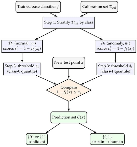
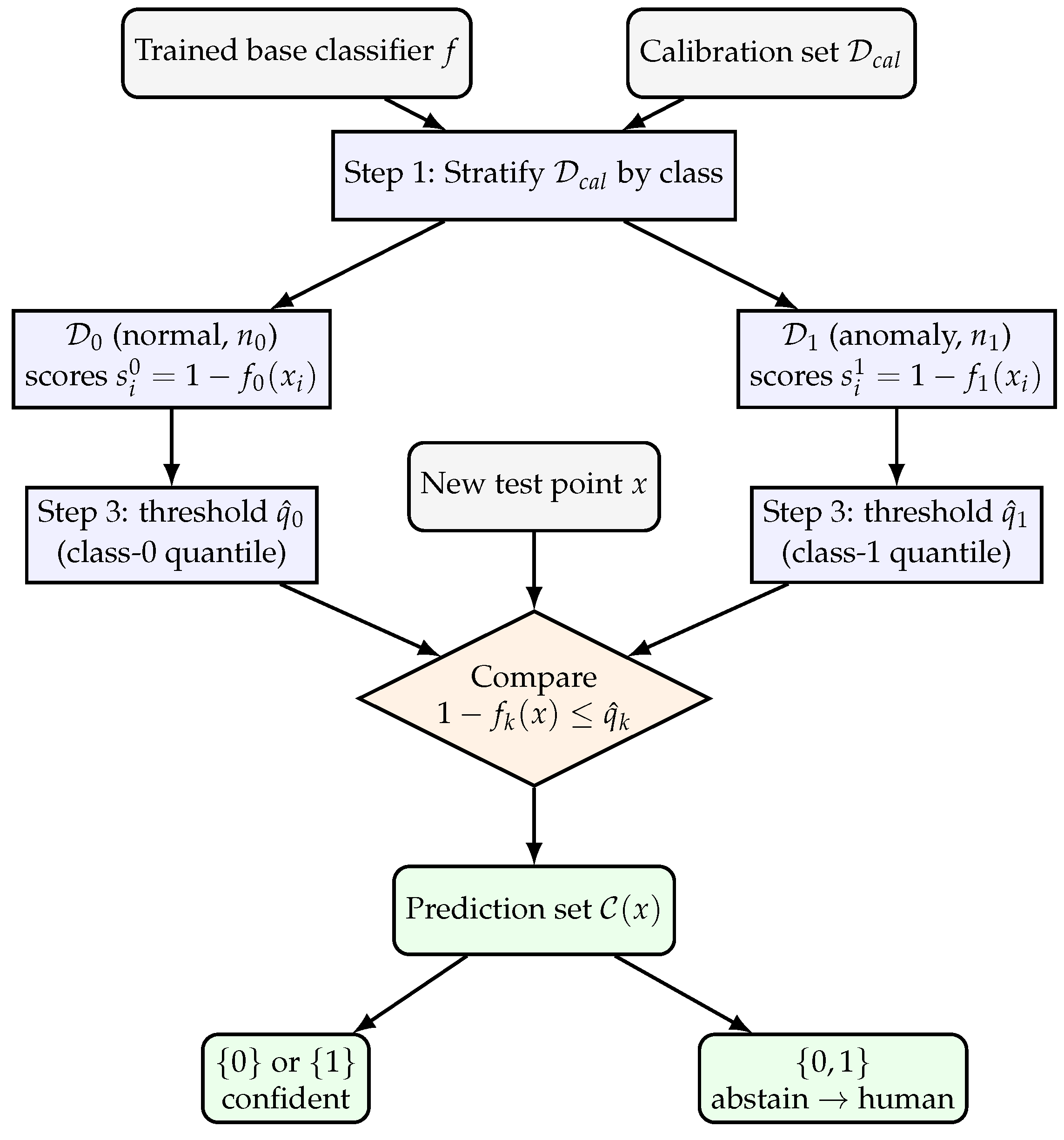
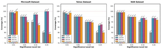
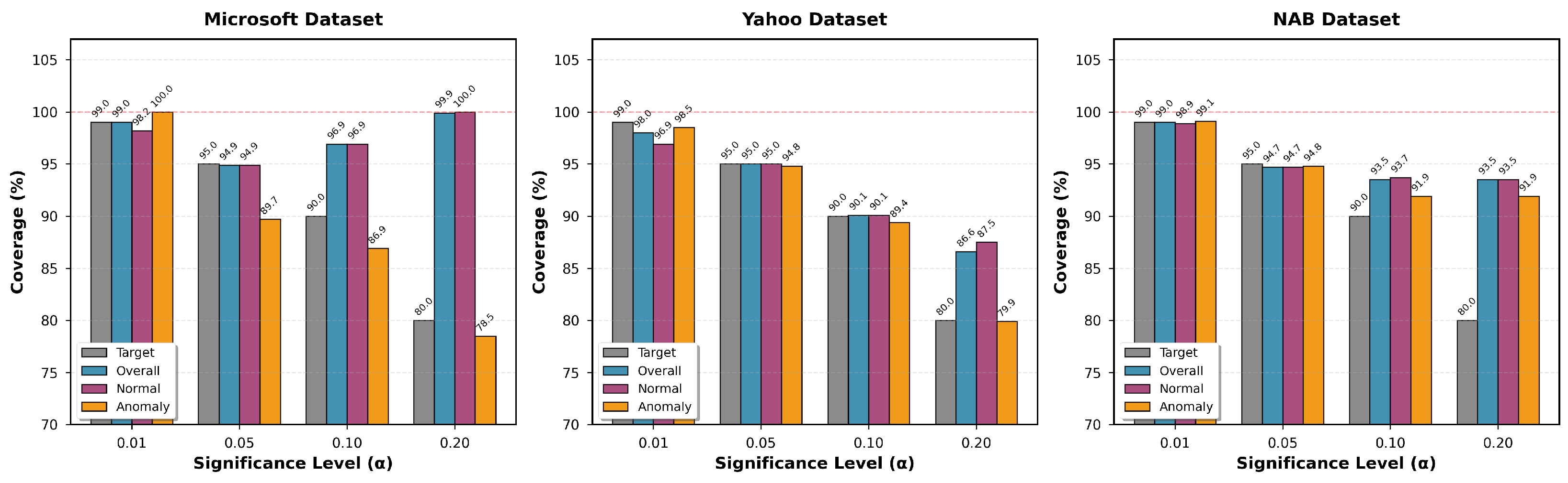
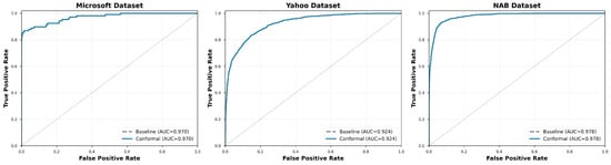
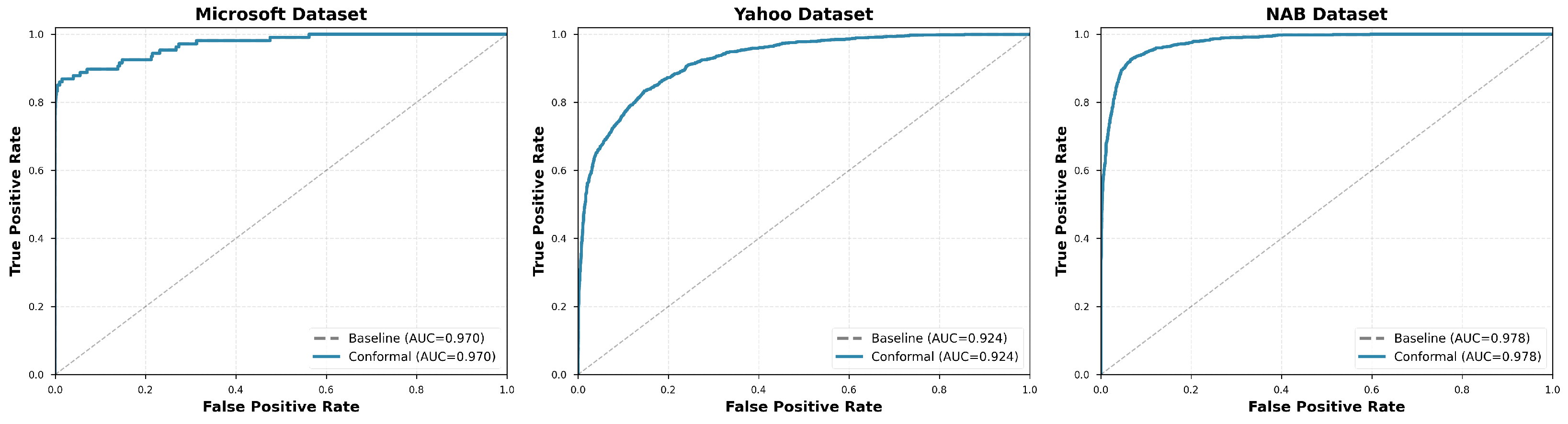
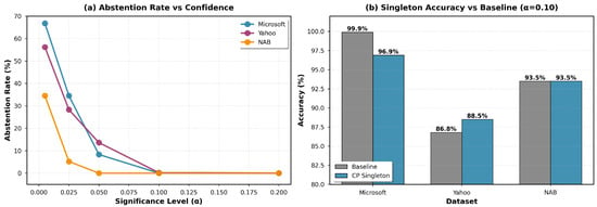
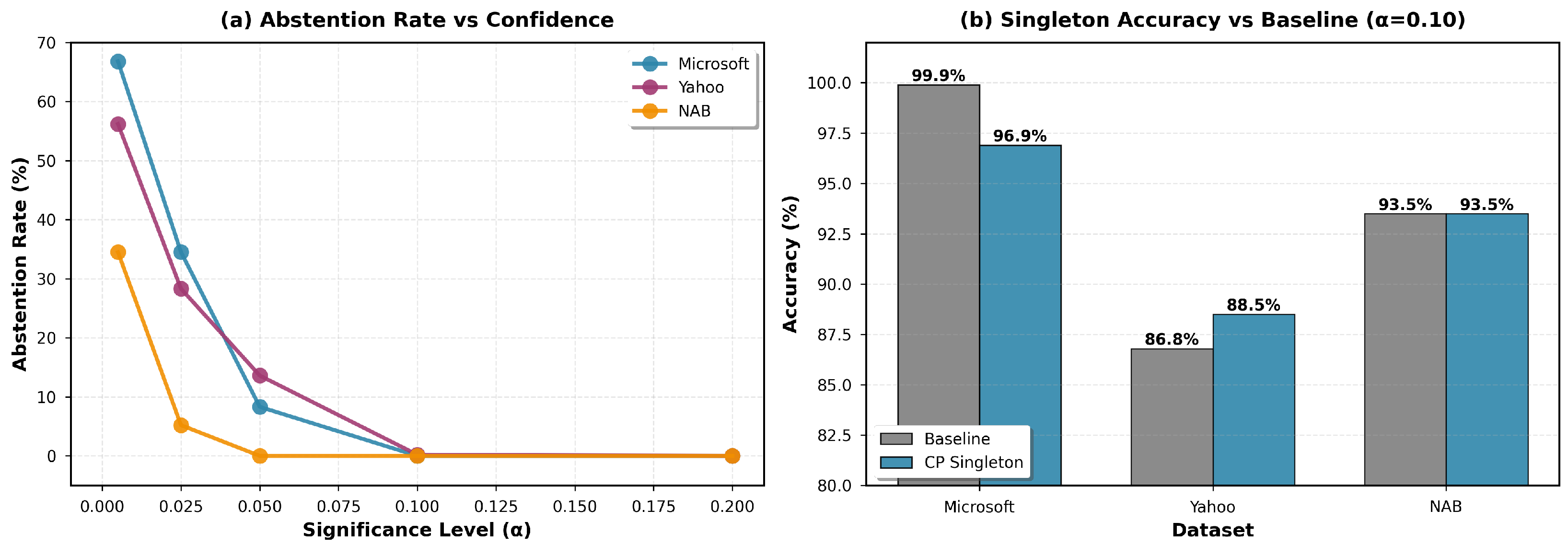
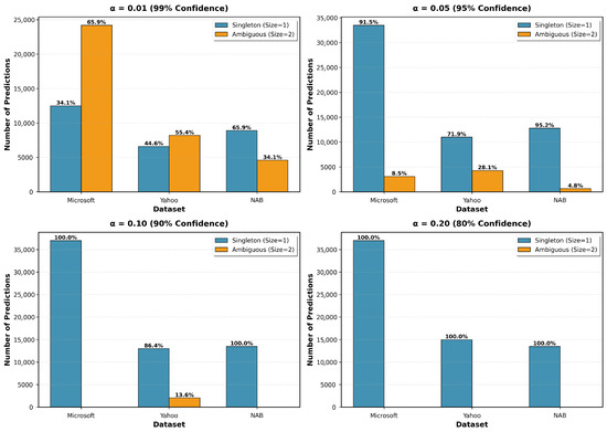
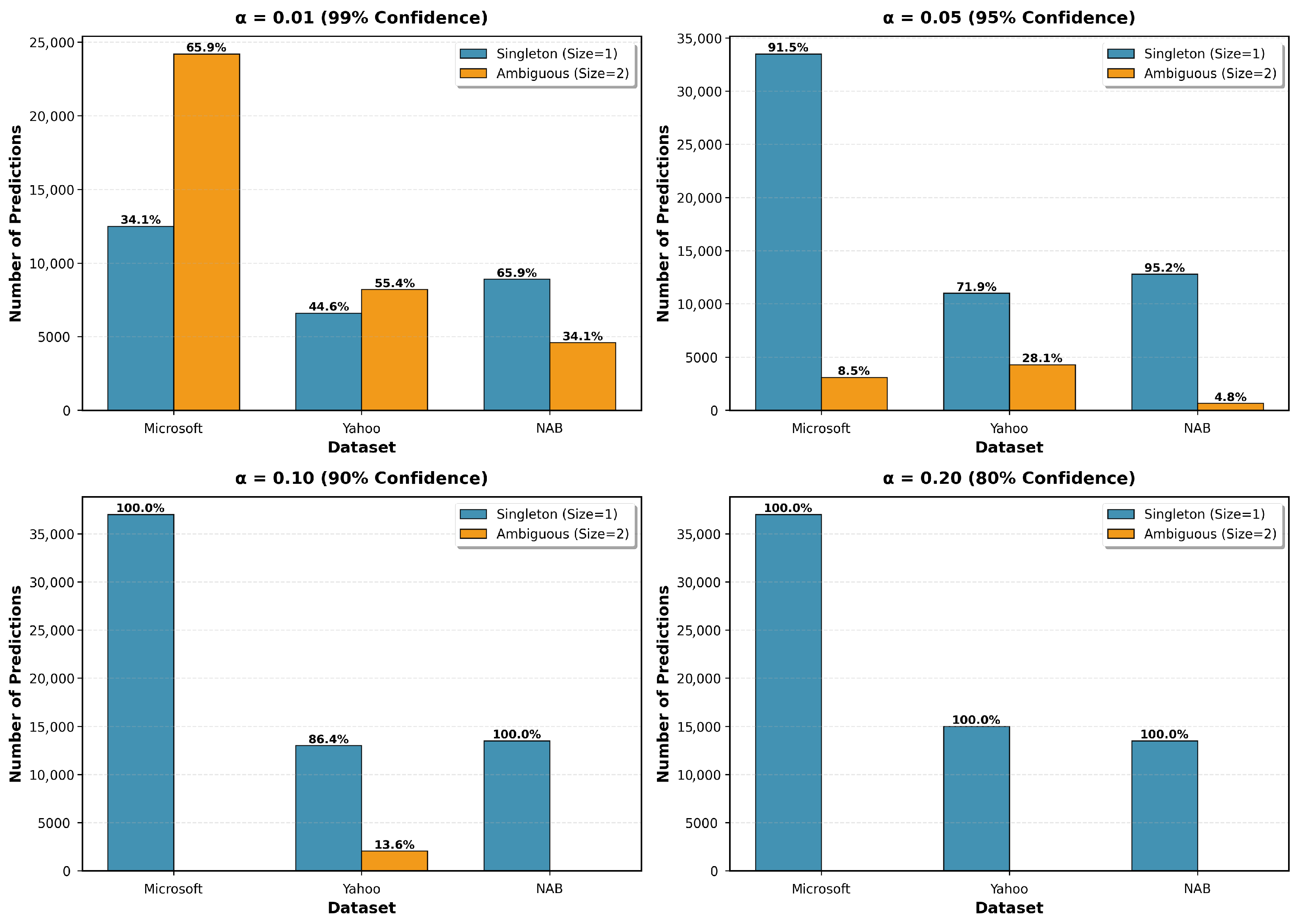
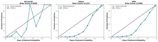
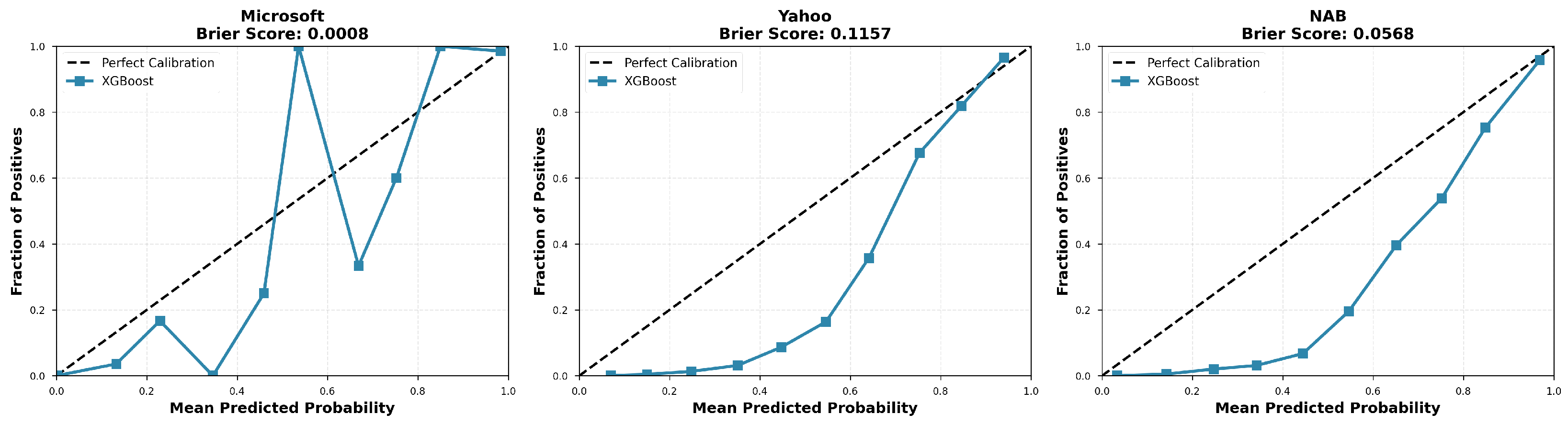

Disclaimer/Publisher’s Note: The statements, opinions and data contained in all publications are solely those of the individual author(s) and contributor(s) and not of MDPI and/or the editor(s). MDPI and/or the editor(s) disclaim responsibility for any injury to people or property resulting from any ideas, methods, instructions or products referred to in the content. |
© 2026 by the author. Licensee MDPI, Basel, Switzerland. This article is an open access article distributed under the terms and conditions of the Creative Commons Attribution (CC BY) license.