Scaling Laws in the Tiny Regime: How Small Models Change Their Mistakes

Abstract

Neural scaling laws describe how model performance improves as a power law with size, but existing work has focused almost entirely on models above 100 M parameters. The regime below 20 million parameters, where TinyML and edge AI systems operate, remains largely unexamined. We train 90 models spanning 22 K to 19.8 M parameters across two architecture families (a plain ConvNet and MobileNetV2) on CIFAR-100, varying width while holding depth and training protocol fixed. Both architectures follow approximate power laws, with exponents of $\alpha =0.156$ (ScaleCNN) and $\alpha =0.106$ (MobileNetV2). However, the power law does not hold uniformly: local exponents decay with scale, and MobileNetV2 saturates at 19.8 M parameters (${\alpha }_{\mathrm{local}}=0.006$), hitting a data wall. The structure of errors also changes with scale. The Jaccard overlap between error sets of the smallest and largest ScaleCNN models is only 0.35; compression changes which inputs are misclassified, not merely how many. Small models develop a triage strategy, concentrating capacity on easy classes (Gini of per-class accuracy: 0.26 at 22 K params vs. 0.09 at 4.7 M) while effectively abandoning the hardest ones (bottom-5 class accuracy: 10% vs. 53%). The smallest models achieve the lowest ECE values (0.013 vs. peak 0.110 at mid-size), reversing the typical overconfidence–capacity relationship, though this partly reflects a global-mean matching artifact rather than well-calibrated per-bin confidence. On CIFAR-100, aggregate accuracy alone is therefore a misleading basis for edge deployment decisions; validation must happen at the target model size. All findings in this study are based on CIFAR-100 (32 × 32, 100 classes); their generalizability to other datasets, resolutions, and architectures remains to be verified.

1. Introduction

Neural scaling laws [1,2] have become one of the more reliable empirical regularities in deep learning. Loss decreases as a power law with model size N, dataset size D, and compute budget C:

$$L\left(N\right)\sim N^{-\alpha }$$

(1)

where $\alpha \approx 0.076$ for language models, with similar values reported for vision transformers [3]. These laws, spanning seven or more orders of magnitude, enabled the strategic scaling decisions behind GPT-3, PaLM, and subsequent frontier models.

Much less is known about the left side of the scaling curve. Below 20 million parameters (the operating point of TinyML systems deployed on microcontrollers with ≤256 KB RAM and ≤1 mW power budgets), we lack answers to basic questions:

• Does the same power law extend to the small-model regime, or does a different scaling relationship govern?
• Does compression merely increase the error rate, or does it fundamentally reshape which inputs the model fails on?
• How do calibration and per-class fairness vary with scale?

These questions matter for deployment. Edge AI systems run in safety-critical contexts (autonomous vehicles, medical devices, industrial monitoring) where the failure distribution matters as much as the failure rate. A model that maintains 88% accuracy after compression but silently shifts all its errors to a specific subpopulation may be more dangerous than one with 85% accuracy and uniformly distributed errors.

The TinyML community typically reports model accuracy at individual operating points. No prior work has systematically varied model size across orders of magnitude on a fixed task to characterize both the functional form and the qualitative changes in error behavior. We set out to do exactly that.

• Contributions.

This paper makes three contributions. First, we provide the first systematic scaling law characterization in the sub-20 M regime, measuring error-rate exponents across nearly three orders of magnitude (22 K–19.8 M parameters) with two architecture families on CIFAR-100. We report architecture-dependent exponents along with a broken power law and architecture-specific saturation. Because prior scaling laws were fit to cross-entropy loss rather than error rate, and these metrics are nonlinearly related, direct numerical comparison of exponents across regimes is approximate. Second, we show that width scaling causes substantial error redistribution: the Jaccard overlap between error sets of the smallest and largest models is only 0.35, well below the 0.58 expected from pure accuracy-driven subset containment. Third, we quantify how small models develop class triage strategies (Gini coefficient of per-class accuracy: 0.26 at 22 K parameters vs. 0.09 at 4.7 M) and document a calibration inversion where the smallest models achieve the lowest ECE, contrary to the usual assumption that overconfidence grows monotonically with capacity.

2. Related Work

• Neural scaling laws.

Kaplan et al. [1] established that language model loss follows power laws in model size, dataset size, and compute, with smooth trends spanning seven orders of magnitude. Hoffmann et al. [2] refined these findings by characterizing compute-optimal training (Chinchilla scaling). Zhai et al. [3] extended scaling analysis to vision transformers. Clark et al. [4] proposed unified scaling laws across modalities. Hestness et al. [5] demonstrated that deep learning scaling is predictable across domains, reporting exponents in the range $\alpha \approx$ 0.07–0.12 for vision tasks above 1 M parameters. However, all of these works focus on the large-model regime (>10 M parameters). The sub-1 M regime relevant to edge deployment has received little attention.

Sharma and Kaplan [6] provided a theoretical grounding for scaling laws by relating the exponent to the intrinsic dimension of the data manifold, predicting $\alpha \approx 4/d$ where d is the manifold dimension. Bahri et al. [7] offered complementary explanations rooted in statistical mechanics. Rosenfeld et al. [8] proposed constructive methods for predicting generalization error across scales. Nakkiran et al. [9] documented deep double descent, where increasing model size can temporarily hurt performance before resuming improvement. Caballero et al. [10] introduced the concept of broken neural scaling laws (BNSL), showing that scaling behavior across wide parameter ranges is better described by smoothly bending power laws than by a single exponent. Our empirical observation of decaying local exponents is consistent with the BNSL framework.

• TinyML and efficient inference.

The TinyML community has developed several complementary techniques for deploying neural networks on microcontrollers: knowledge distillation [11], structured pruning [12], quantization-aware training [13], and neural architecture search for constrained devices [14,15]. Recent work has established standardized benchmarks for sub-milliwatt inference [16], demonstrated on-device training under 256 KB memory [17], and surveyed the rapidly growing TinyML ecosystem [18,19]. Hardware-aware methods now routinely target sub-1 M parameter budgets with differentiable pruning [20]. However, these works optimize for accuracy at a specific target size but do not characterize the functional relationship between accuracy and size across scales. We aim to fill that gap by measuring how accuracy, error distribution, and calibration evolve as model size varies continuously.

• Emergent capabilities and phase transitions.

Wei et al. [21] documented emergent capabilities in large language models that appear discontinuously at critical scales. Schaeffer et al. [22] argued that some apparent emergence is an artifact of nonlinear evaluation metrics. Our work addresses the opposite end of the scale: we study capability degradation as models shrink, focusing on per-class performance, error redistribution, and calibration rather than aggregate metrics.

• Compression and fairness.

Pruning disproportionately affects underrepresented classes, as Hooker et al. [23] showed through the concept of “Pruning Identified Exemplars”. Liebenwein et al. [24] extended this to show that pruning effects go beyond test accuracy. Our work builds on these findings: we quantify error redistribution across the full scaling range using Jaccard overlap rather than individual exemplars, we show that scale drives error patterns more than architecture choice, and we characterize the class-level triage strategy that small models adopt.

• Calibration.

Modern neural networks are systematically miscalibrated, with overconfidence increasing with capacity [25]. Our results partially contradict this monotonic trend: in the small-model regime, the smallest models register the lowest ECE values, and miscalibration follows an inverted-U pattern rather than increasing monotonically with size, although as we discuss in Section 5.6 this advantage is partly a global-mean matching artifact rather than evidence of well-calibrated per-bin confidence. Alabdulmohsin et al. [26] revisited scaling laws for vision and language with a focus on metrics beyond loss, which is close in spirit to our multi-metric approach.

3. Theoretical Framework: Spectral Capacity Theory

This section develops a spectral capacity model that relates the scaling exponent to properties of the data and the network. We present it not as an independent predictive theory but as a post hoc consistency check: the framework is used to verify whether the measured exponents are compatible with known spectral properties of natural images and reasonable assumptions about network capacity. As discussed in Section 3.4, the reconciliation remains partially circular because the rank efficiency parameter $\gamma$ is back-calculated from the measured exponents rather than measured independently.

3.1. Data Spectral Structure

Natural data distributions exhibit scale-free spectral structure. The eigenvalues of the data covariance matrix $\Sigma$ follow a power-law decay:

$${\lambda }_k\sim k^{-\beta }$$

(2)

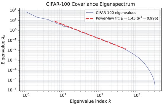
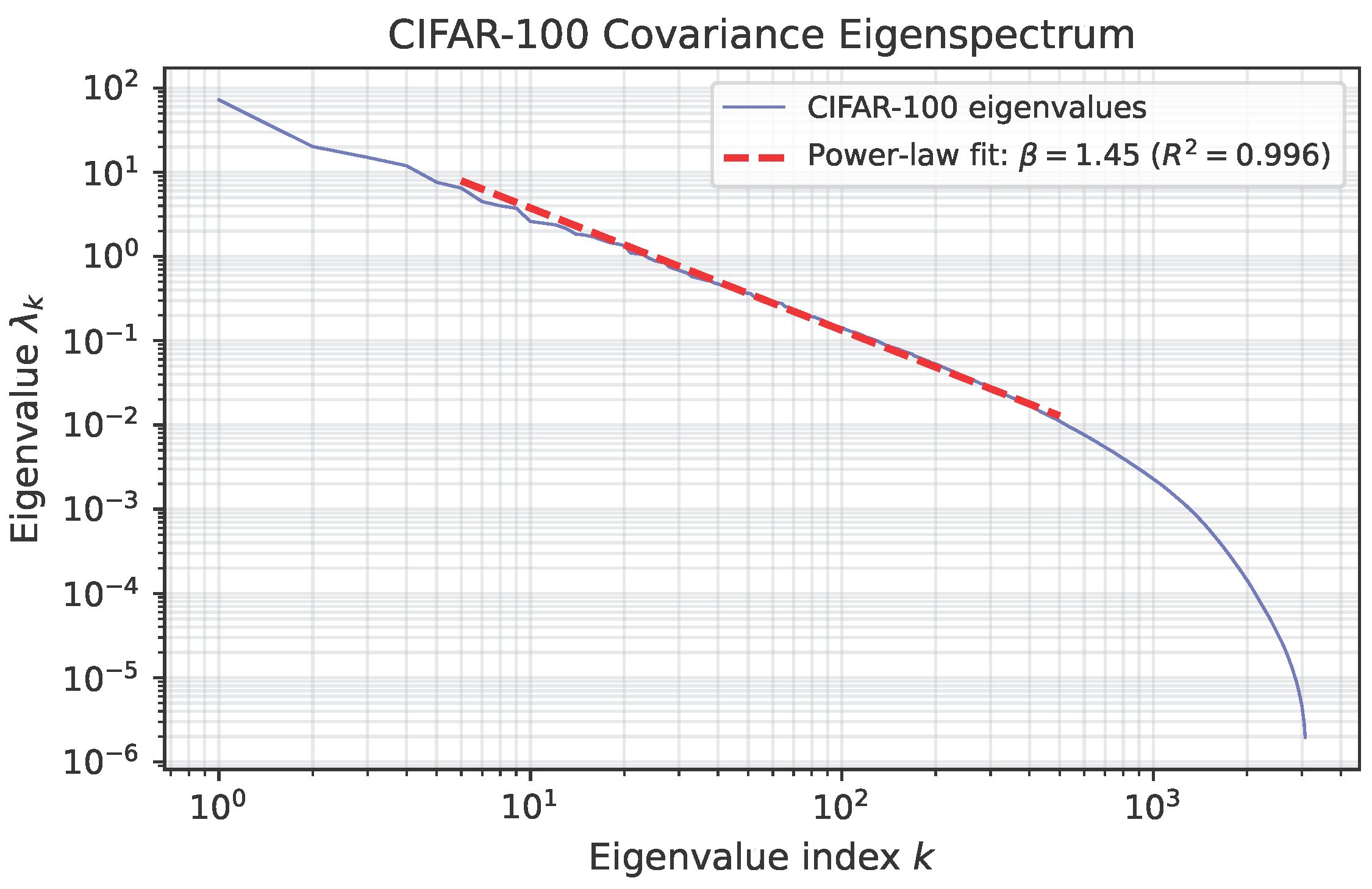
where $\beta >1$ is the spectral decay exponent and k indexes eigenvalues in decreasing order. For natural images at native resolution, $\beta \approx$ 1.0–1.2 [27,28]. We directly measured $\beta$ from the eigenspectrum of the CIFAR-100 training set covariance matrix (50,000 images, 3072 dimensions). Fitting a power law to eigenvalues k = 5–500 yields ${\beta }_{\mathrm{CIFAR}}=1.45$ ($R^2=0.996$); the fit is robust across ranges ($\beta$ = 1.35–1.45 for $k\in [2,200]$ to $[5,500]$). Figure 1 shows the eigenspectrum and fit. The steeper decay compared to natural images at native resolution reflects CIFAR-100’s 32 × 32 downsampling, which removes high-frequency content and steepens spectral rolloff.

Figure 1. Eigenvalue spectrum of the CIFAR-100 training set covariance matrix. The power-law fit ${\lambda }_k\sim k^{-1.45}$ ($R^2=0.996$, fit range k = 5–500) confirms steeper spectral decay than reported for natural images at native resolution ($\beta \approx$ 1.0–1.2).

3.2. Effective Rank and the Parameter-to-Capacity Mapping

A neural network with N parameters can effectively represent data projected onto a subspace of dimensionality $K\left(N\right)$, which we term the effective rank. For convolutional networks with width multiplier m:

$$N\sim m^2·{\left(\mathrm{kernel}\mathrm{size}\right)}^2·d,K\sim m·r$$

(3)

where d is depth and r is spatial resolution. In general:

$$K\left(N\right)\sim N^{\gamma }$$

(4)

where $\gamma \in (0,1)$ is the rank efficiency exponent. For most practical architectures, $\gamma \approx 0.5$.

3.3. Deriving the Scaling Exponent

A model with effective rank $K\left(N\right)$ captures the top $K\left(N\right)$ eigenmodes of the data distribution. The residual loss is

$$L\left(N\right)=\sum _{k>K\left(N\right)}{\lambda }_k\approx {\int }_{K\left(N\right)}^{\infty }{k}^{-\beta }dk={\displaystyle \frac{K{\left(N\right)}^{1-\beta }}{\beta -1}}$$

(5)

Substituting $K\left(N\right)\sim N^{\gamma }$:

$$\begin{array}{|c|}\hline L\left(N\right)\sim N^{-\alpha },\mathrm{where}\alpha =\gamma (\beta -1)\\ \hline\end{array}$$

(6)

This predicts the scaling exponent from two independently measurable quantities: $\beta$ (a data property) and $\gamma$ (an architecture property).

3.4. Theoretical Prediction vs. Empirical Exponents

For natural images at native resolution with $\beta \approx 1.1$ and convolutional networks with $\gamma \approx 0.5$, the spectral capacity theory predicts $\alpha \approx 0.05$. Our measured exponents ($\alpha =0.156$ for ScaleCNN and $\alpha =0.106$ for MobileNetV2) are 2–3× larger than this prediction. The resolution comes from the direct eigenspectrum measurement in Section 3.1: CIFAR-100’s measured ${\beta }_{\mathrm{CIFAR}}=1.45$ is steeper than the literature value for natural images at native resolution. With this measured $\beta$, the theory predicts $\alpha =0.5\times 0.45=0.225$ for $\gamma =0.5$. The ScaleCNN exponent ($0.156$) implies ${\gamma }_{\mathrm{CNN}}=0.156/0.45=0.35$, and the MobileNetV2 exponent ($0.106$) implies ${\gamma }_{\mathrm{MobNet}}=0.106/0.45=0.24$. These $\gamma$ values are below the theoretical maximum of 0.5, consistent with the expectation that real networks convert parameters to effective rank less efficiently than the linear bound. The gap between the two architectures reflects differences in rank efficiency: ScaleCNN’s simple structure converts parameters to effective rank more efficiently than MobileNetV2’s depthwise separable design, which spends parameters on bottleneck projections and expansion layers.

The framework is consistent with the functional form (power law with architecture-dependent exponent) and the qualitative ordering (${\alpha }_{\mathrm{CNN}}>{\alpha }_{\mathrm{MobNet}}$). With the directly measured $\beta$, the remaining circularity is reduced to the $\gamma$ parameter, which is still inferred from the measured $\alpha$ rather than measured independently. To fully close this loop, future work should measure $\gamma$ directly (e.g., by computing the stable rank of intermediate activation matrices across trained networks of varying width), enabling a quantitative test of Equation (6) without any back-calculated parameters.

4. Experimental Setup

4.1. Hypotheses

We organize the experiments around two hypotheses.

H1 (Power-law scaling).

If the sub-20 M regime follows the same scaling form as larger models, then $log\left(\mathit{error}\mathit{rate}\right)$ vs. $log\left(N\right)$ should be approximately linear across ≥2 orders of magnitude. We consider the hypothesis unsupported if $R^2<0.9$ or if residuals show systematic non-monotonic structure.

H2 (Error redistribution).

If compression merely adds errors without changing which inputs fail, then the Jaccard overlap between error sets at different model sizes should remain high. We consider the hypothesis unsupported if overlap stays above 0.90 across all comparisons.

4.2. Model Families

We use two architecture families to span complementary parameter ranges:

• ScaleCNN.

This is a plain 4-block convolutional network with channels $[c,2c,4c,8c]$, where each block contains two conv-BN-ReLU layers followed by spatial pooling. The classifier is a single linear layer. Base channel widths $c\in \{4,8,12,16,24,32,48,64\}$ yield 8 model sizes from 22 K to 4.7 M parameters with clean quadratic scaling ($N\propto c^2$). This architecture was chosen for its interpretable capacity scaling and absence of structural bottlenecks.

• MobileNetV2.

This is the standard inverted-residual architecture [29] with ten width multipliers $m\in \{0.10,0.15,0.25,0.35,0.50,0.75,1.00,1.50,2.00,3.00\}$, yielding 10 model sizes from 214 K to 19.8 M parameters. The first convolutional layer’s stride is reduced from 2 to 1 to accommodate CIFAR-100’s 32 × 32 input resolution.

Together, the two families provide 18 configurations spanning 22 K to 19.8 M parameters (nearly three orders of magnitude). Table 1 summarizes the experimental grid.

Table 1. Experimental configurations: 18 model sizes × 5 seeds = 90 runs.

Architecture	Size Parameter	Configs	Param Range
ScaleCNN	Base channels $c\in \{4,8,\dots ,64\}$	8	22 K–4.7 M
MobileNetV2	Width mult. $m\in \{0.10,\dots ,3.00\}$	10	214 K–19.8 M
Total		18	22 K–19.8 M

4.3. Dataset: CIFAR-100

We evaluate on CIFAR-100, which provides 50,000 training images and 10,000 test images across 100 balanced classes at 32 × 32 resolution. CIFAR-100 was chosen because (a) its 100 fine-grained classes create meaningful per-class variation, enabling the class triage analysis; (b) its moderate training set size creates natural saturation behavior at the upper end of our parameter range; and (c) it is a widely used benchmark in the TinyML and model compression literature.

4.4. Training Protocol

All models within an architecture family share identical training hyperparameters: SGD with momentum 0.9, weight decay $5\times {10}^{-4}$, cosine annealing from ${10}^{-1}$ to ${10}^{-5}$ over 200 epochs, batch size 128, and data augmentation (random crop with padding 4, horizontal flip, Cutout [30] with 8 × 8 patches). Each configuration is trained with five random seeds (0–4). All results report mean ± standard deviation across seeds.

4.5. Measurements

At each operating point, we measure

• Performance: Top-1 accuracy, top-5 accuracy, per-class accuracy vector (100 values).
• Error characterization: Per-sample correct/incorrect mask (for Jaccard overlap computation), per-class error rates, Gini coefficient of per-class accuracy.
• Calibration: Expected calibration error (ECE, 15 bins), mean confidence on correct and incorrect predictions.

Evaluation uses the trained model at epoch 200 (no early stopping or best-checkpoint selection) to ensure all models are compared at the same training budget.

5. Results

5.1. Power-Law Scaling

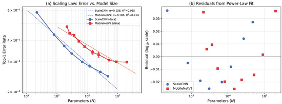
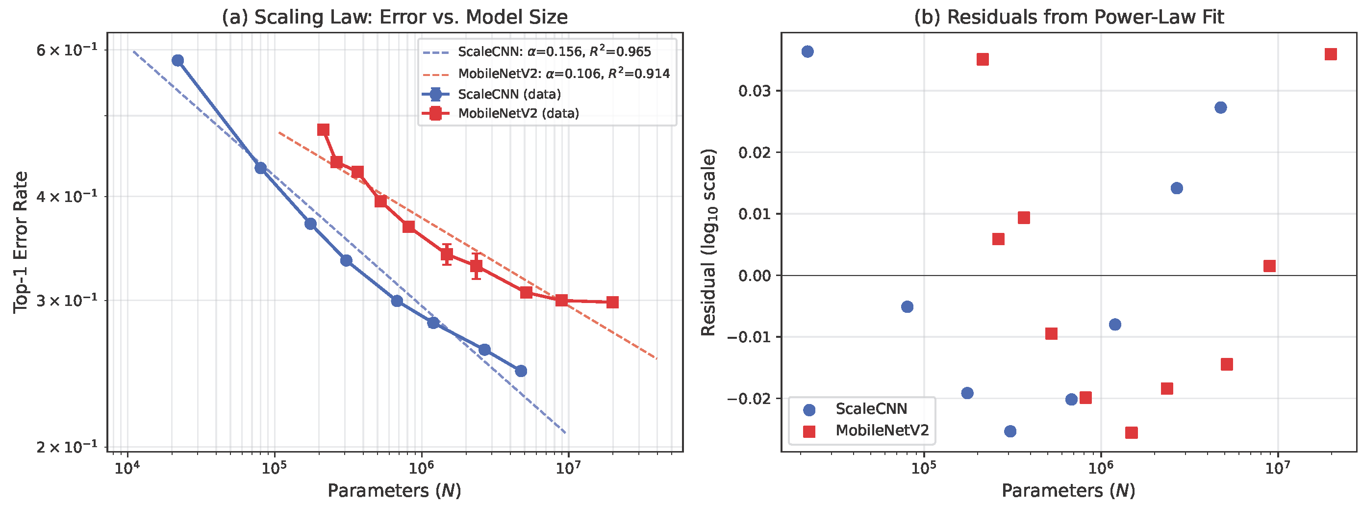
Figure 2 plots top-1 error rate vs. parameter count on log–log axes for both architecture families. Both exhibit approximate power-law behavior:

$$\begin{array}{cc}\hfill \mathrm{ScaleCNN}:& \mathrm{error}\sim N^{-0.156},R^2=0.965\hfill \end{array}$$

(7)

$$\begin{array}{cc}\hfill \mathrm{MobileNetV}2:& \mathrm{error}\sim N^{-0.106},R^2=0.914\hfill \end{array}$$

(8)

Figure 2. (a) Log–log plot of top-1 error rate vs. parameter count for ScaleCNN (blue) and MobileNetV2 (red). Error bars: $\pm 1$ std across 5 seeds. Dashed lines: power-law fits. (b) Residuals from the power-law fit showing systematic curvature (broken power law).

ScaleCNN scales 47% more efficiently per parameter than MobileNetV2, despite the latter being engineered for inference efficiency. We attribute the gap to MobileNetV2’s structural overhead: depthwise separable convolutions, expansion layers, and bottleneck projections consume parameters without proportionally increasing representational capacity at small widths.

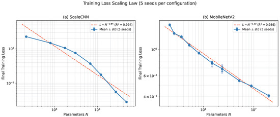
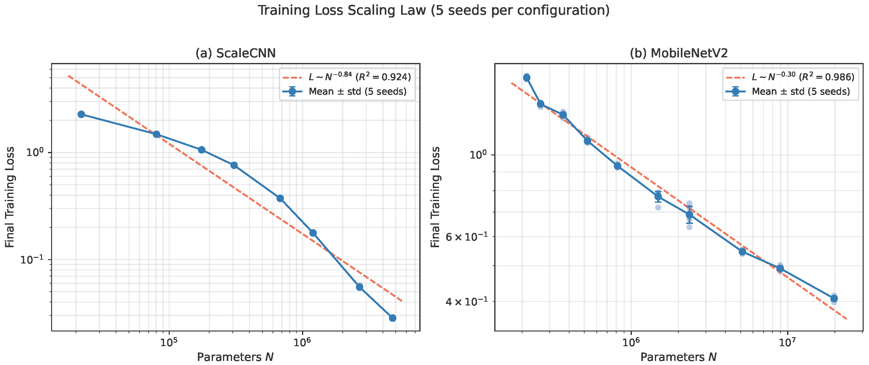
For reference, Kaplan et al. [1] reported $\alpha \approx 0.076$ for large language models and Hestness et al. [5] reported $\alpha \approx$ 0.07–0.12 for vision models above 1 M parameters. Our error-rate exponents are numerically larger; however, because those prior works fit power laws to cross-entropy loss rather than error rate, and the two metrics are nonlinearly related, the numerical comparison is only approximate. Our own data illustrate this divergence: the training-loss exponent for ScaleCNN (${\alpha }_{\mathrm{train}}=0.84$, $R^2=0.924$) is $\sim 5\times$ the error-rate exponent ($0.156$), which shows that exponents are metric-dependent. Figure 3 shows the training loss scaling across all five seeds for both architectures, demonstrating stable power-law behavior with low cross-seed variance (std $<0.04$ at all operating points).

Figure 3. Training loss scaling law across five seeds per configuration. Individual seeds are shown as faint dots; means ± std are plotted with error bars. (a) ScaleCNN: ${\alpha }_{\mathrm{train}}=0.84$ ($R^2=0.924$). (b) MobileNetV2: ${\alpha }_{\mathrm{train}}=0.30$ ($R^2=0.986$). The low cross-seed variance confirms algorithmic stability across the full parameter range.

Table 2 provides the full results.

Table 2. Full results: 90 runs (5 seeds each). Accuracy is top-1 on CIFAR-100 test set.

Arch	Config	Params	MACs (M)	Accuracy (%)	ECE
ScaleCNN	$c=4$	21,936	1.8	$41.71\pm 0.45$	0.013
	$c=8$	80,348	7.0	$56.73\pm 0.40$	0.037
	$c=12$	175,336	15.5	$62.91\pm 0.17$	0.059
	$c=16$	306,900	27.4	$66.49\pm 0.23$	0.073
	$c=24$	679,756	61.2	$70.05\pm 0.29$	0.098
	$c=32$	1,198,916	108.6	$71.81\pm 0.33$	0.110
	$c=48$	2,676,148	243.8	$73.82\pm 0.28$	0.102
	$c=64$	4,738,596	433.0	$75.32\pm 0.22$	0.082
MobNetV2	$m=0.10$	214,180	5.3	$51.91\pm 0.42$	0.016
	$m=0.15$	262,596	8.1	$55.99\pm 0.37$	0.021
	$m=0.25$	366,212	14.5	$57.17\pm 0.38$	0.023
	$m=0.35$	524,228	22.8	$60.52\pm 0.52$	0.033
	$m=0.50$	815,780	40.1	$63.21\pm 0.34$	0.038
	$m=0.75$	1,483,524	78.6	$65.92\pm 0.98$	0.045
	$m=1.00$	2,351,972	131.4	$67.00\pm 1.16$	0.053
	$m=1.50$	5,129,252	280.3	$69.34\pm 0.23$	0.058
	$m=2.00$	8,953,188	490.7	$70.01\pm 0.12$	0.059
	$m=3.00$	19,803,748	1089.2	$70.15\pm 0.28$	0.072

As an illustrative comparison, ScaleCNN at $c=64$ (4.7 M parameters, 75.32% accuracy) outperforms MobileNetV2 at $m=3.0$ (19.8 M parameters, 70.15% accuracy) by over 5 percentage points with 4.2× fewer parameters. At this dataset scale, the plain convolutional architecture achieves higher parameter efficiency than the architecture specifically designed for efficient inference.

5.2. Broken Power Law: Local Exponent Decay

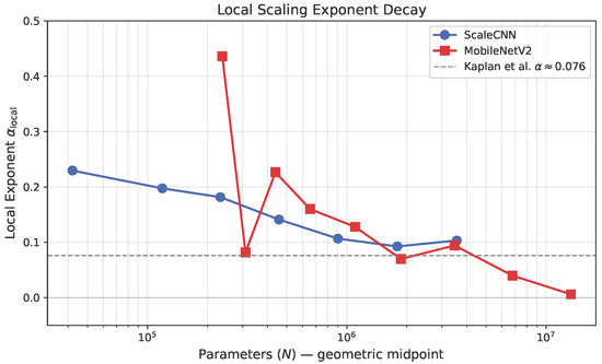
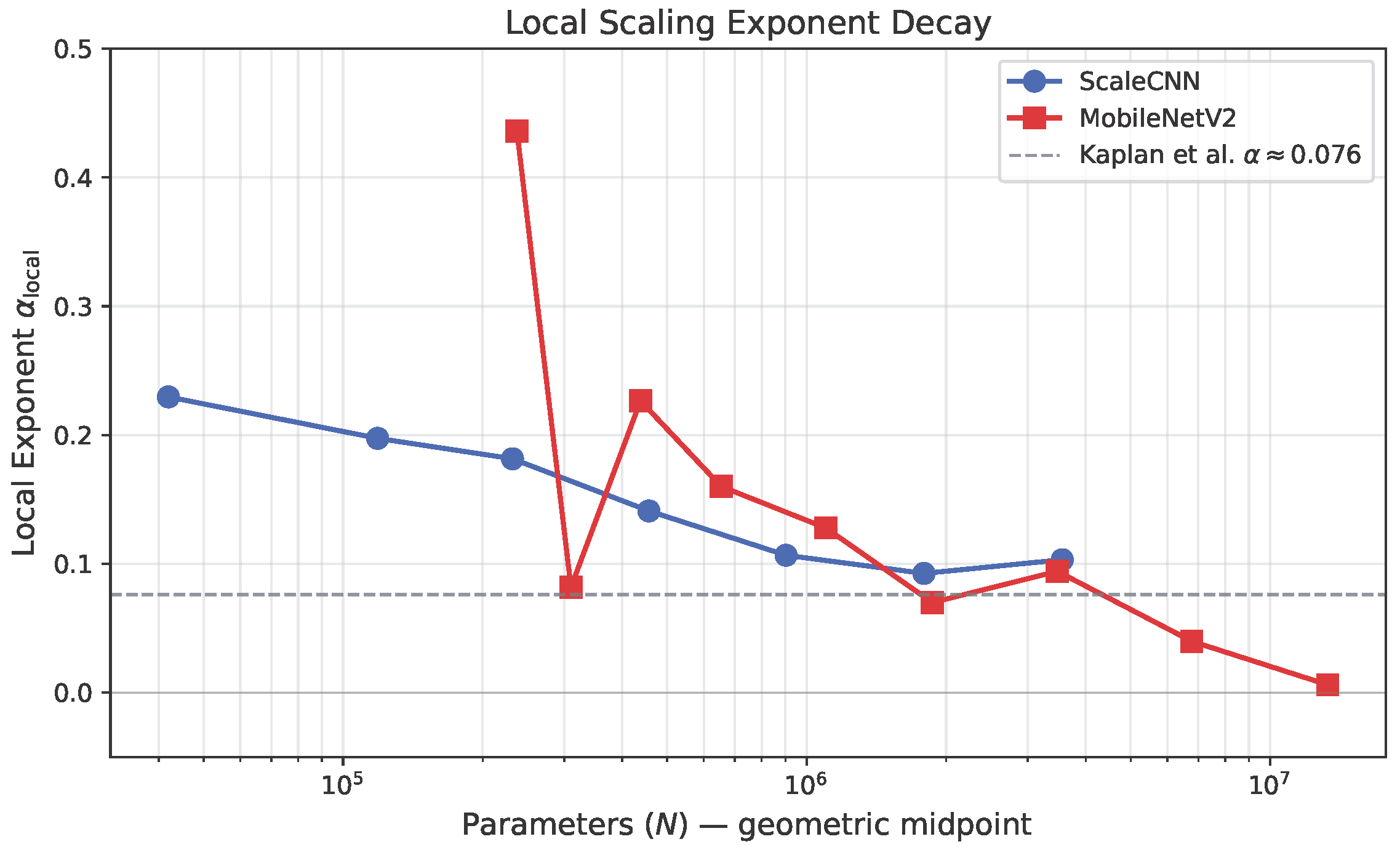
A single exponent summarizes the full range but hides structure. Figure 4 shows what happens when we compute the local scaling exponent ${\alpha }_{\mathrm{local}}$ as the finite-difference slope between adjacent model sizes: it decays with scale.

Figure 4. Local scaling exponent ${\alpha }_{\mathrm{local}}$ vs. parameter count. ScaleCNN shows smooth monotonic decay from 0.23 to 0.10. MobileNetV2 shows oscillatory behavior followed by collapse to 0.006. The Kaplan et al. [1] reference exponent ($\alpha \approx 0.076$) is shown as a dashed line.

ScaleCNN exhibits smooth, monotonic decay: the local exponent falls from 0.23 in the tiny regime (<100 K parameters) to 0.10 near 5 M parameters, approaching the range reported for larger vision models. This is consistent with a smoothly bending power law (the BNSL framework of Caballero et al. [10]) rather than a sharp regime change.

MobileNetV2 behaves differently. The local exponent oscillates wildly at small widths, jumping from 0.44 ($m=0.10\to 0.15$) down to 0.08 ($m=0.15\to 0.25$) and back up to 0.23 ($m=0.25\to 0.35$). We initially thought this was a seed variance artifact and reran the smallest MobileNetV2 configurations, but the pattern was stable across all five seeds (standard deviation of accuracy < 0.52% at each width). We attribute this oscillation to the inverted-residual bottleneck structure. Table 3 lists the narrowest bottleneck dimension $\lfloor 16·m\rfloor$ for each width multiplier:

Table 3. MobileNetV2 first-layer bottleneck dimension $\lfloor 16·m\rfloor$, local exponent ${\alpha }_{\mathrm{local}}$, and final training loss drop $\Delta L_{\mathrm{train}}$ for adjacent transitions.

Width m	0.10	0.15	0.25	0.35	0.50
Bottleneck dim	1	2	4	5	8
${\alpha }_{\mathrm{local}}$	—	0.44	0.08	0.23	0.15
$\Delta L_{\mathrm{train}}$	—	$-0.31$	$-0.08$	$-0.19$	$-0.12$

At $m=0.10$, the narrowest bottleneck layers have only one channel, so the $m=0.10\to 0.15$ transition doubles the bottleneck from one to two channels, producing a disproportionately large capacity gain (${\alpha }_{\mathrm{local}}=0.44$, $\Delta L_{\mathrm{train}}=-0.31$). At $m=0.25$, the bottleneck reaches four channels, wide enough that further widening mainly adds redundant parameters in the expansion layers, temporarily flattening the exponent (${\alpha }_{\mathrm{local}}=0.08$, $\Delta L_{\mathrm{train}}=-0.08$). Above $m=0.50$ (bottleneck ≥8), all layers are wide enough that structural effects wash out, and the exponent declines monotonically toward zero.

In the tiny-model regime (<100 K parameters), scaling is 2.5–3× steeper than in the standard regime, indicating that each added parameter buys more accuracy at the smallest scales.

5.3. MobileNetV2 Saturation: The Data Wall

The final MobileNetV2 data points reveal complete architectural saturation on CIFAR-100, summarized in Table 4.

Table 4. MobileNetV2 transition-by-transition accuracy gains and local exponents at the upper end of the parameter range, illustrating the data wall at $m\ge 2.0$.

Transition	Accuracy Gain	${\mathit{\alpha }}_{\mathbf{local}}$	Regime
$m=1.0\to 1.5$	$+2.34\%$	0.094	Normal scaling
$m=1.5\to 2.0$	$+0.67\%$	0.040	Diminishing returns
$m=2.0\to 3.0$	$+0.14\%$	0.006	Saturation

Doubling from 9 M to 20 M parameters yields only 0.14% accuracy gain (${\alpha }_{\mathrm{local}}=0.006$), effectively zero. At $m=3.0$, the parameter-to-sample ratio is 396:1, and the model is massively overparameterized for CIFAR-100’s 50 K training set. This saturation is not observed in ScaleCNN at comparable parameter counts ($c=48\to 64$ still shows ${\alpha }_{\mathrm{local}}=0.10$ at 4.7 M parameters), suggesting the saturation is architecture-specific: MobileNetV2’s depthwise separable design hits a capacity ceiling earlier than a simple ConvNet on this dataset.

5.4. Error Redistribution

The scaling exponent tells us how much worse a smaller model gets. It says nothing about how it gets worse, and in practice the “how” matters more. Shrinking a model does not simply raise the error count; it rearranges the set of inputs that fail.

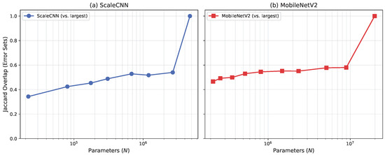
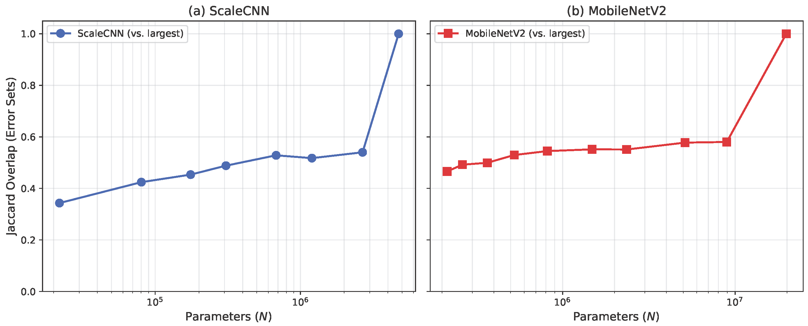
We compute the Jaccard index between error sets of each model and the largest model in its architecture family across all five seeds. Figure 5 shows the result.

Figure 5. Jaccard overlap between error sets of each model and the largest model in its family, plotted against parameter count (log scale, two panels). The left panel (a) shows ScaleCNN ($c=4$ vs. $c=64$ yields Jaccard = 0.35); the right panel (b) shows MobileNetV2, where overlap stabilizes above $m=1.5$ as the architecture saturates. Adjacent model sizes share 65–72% of errors in both families.

The ScaleCNN Jaccard matrix shows that only 36% of errors overlap between the smallest ($c=4$, 22 K params) and largest ($c=64$, 4.7 M params) models. A 200× compression changes the identity of 64% of errors. Adjacent sizes share 65–72% of errors, showing that error redistribution accumulates gradually across the scaling range.

Cross-architecture analysis shows that two different architectures at similar parameter counts make more similar errors than the same architecture at different sizes. Table 5 presents the cross-architecture Jaccard overlaps at matched parameter counts, averaged across all five seeds, confirming that scale drives error patterns more than architecture choice.

Table 5. Cross-architecture Jaccard overlap at matched parameter counts (mean ± std across 5 seeds, ratio $<2\times$). Cross-architecture overlap at similar sizes exceeds within-architecture overlap across distant sizes, indicating that scale drives error patterns more than architecture choice.

ScaleCNN	MobileNetV2	CNN Params	Mob Params	Jaccard
$c=12$	$m=0.10$	175 K	214 K	$0.553\pm 0.004$
$c=16$	$m=0.15$	307 K	263 K	$0.528\pm 0.002$
$c=16$	$m=0.25$	307 K	366 K	$0.533\pm 0.002$
$c=24$	$m=0.35$	680 K	524 K	$0.508\pm 0.006$
$c=24$	$m=0.50$	680 K	816 K	$0.515\pm 0.005$
$c=32$	$m=0.75$	1.2 M	1.5 M	$0.503\pm 0.009$
$c=48$	$m=1.00$	2.7 M	2.4 M	$0.491\pm 0.005$
$c=48$	$m=1.50$	2.7 M	5.1 M	$0.496\pm 0.004$
$c=64$	$m=1.00$	4.7 M	2.4 M	$0.476\pm 0.008$
$c=64$	$m=1.50$	4.7 M	5.1 M	$0.482\pm 0.004$
$c=64$	$m=2.00$	4.7 M	9.0 M	$0.488\pm 0.003$
Mean cross-arch Jaccard				$0.507\pm 0.005$
Mean within-arch adjacent Jaccard (ScaleCNN)				$0.567\pm 0.022$
Mean within-arch adjacent Jaccard (MobileNetV2)				$0.617\pm 0.033$

The MobileNetV2 saturation effect is visible in the Jaccard data: $m=2.0$ and $m=3.0$ have nearly identical cross-architecture overlap values (e.g., vs. ScaleCNN $c=64$: $0.488\pm 0.003$ vs. $0.482\pm 0.004$), which means doubling parameters changes almost nothing about the error pattern once saturation is reached. The low standard deviations across seeds (0.002–0.009) confirm that error redistribution is a stable structural phenomenon, not an artifact of random initialization.

5.5. Class Triage: The Fairness Cost of Compression

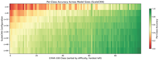
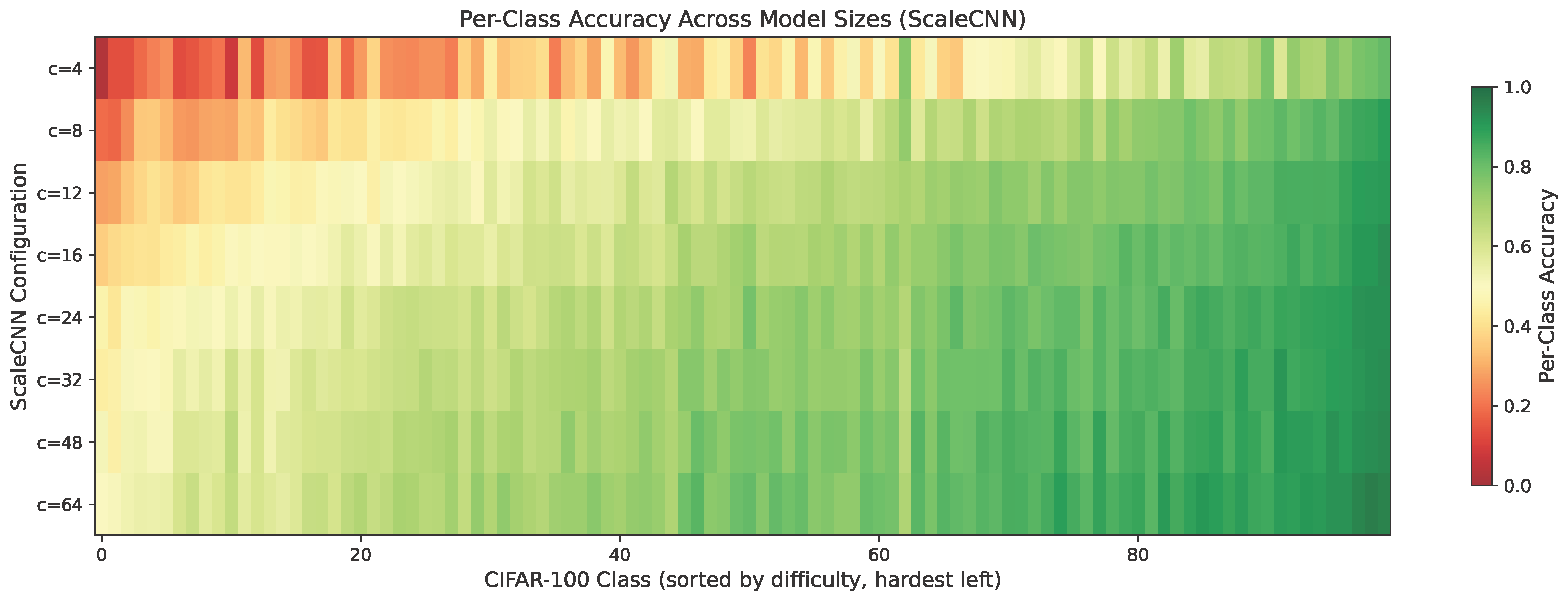
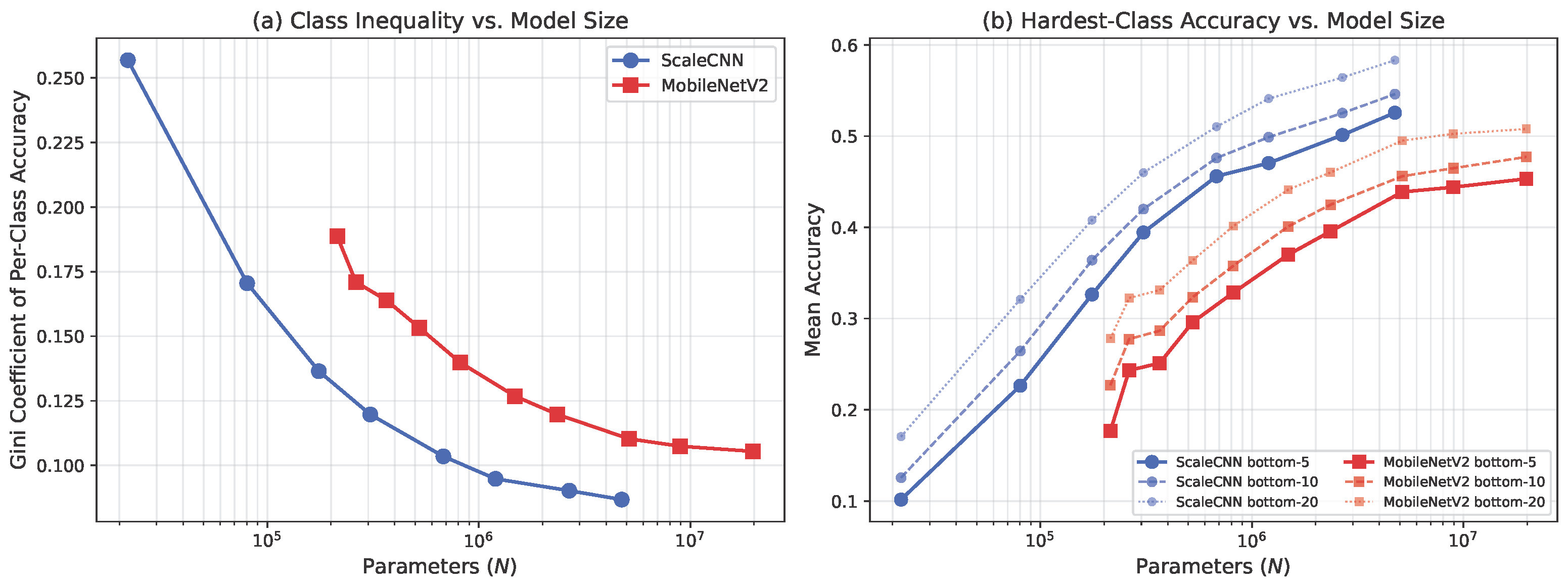
Small models develop an extreme triage strategy: they concentrate representational capacity on easy classes and all but abandon the hardest ones. Figure 6 and Figure 7 quantify this effect.

Figure 6. Per-class accuracy heatmap for ScaleCNN (classes sorted by difficulty, hardest left). Small models show extreme variation: near-zero accuracy on the hardest classes, near-80% on the easiest.

Figure 7. (a) Gini coefficient of per-class accuracy vs. model size. Small models exhibit high inequality (Gini = 0.26), which drops to 0.09 as models grow. (b) Mean accuracy of the hardest 5, 10, and 20 classes. Bottom-5 accuracy rises from 10% to 53% with scale.

The Gini coefficient drops 3× as models grow from 22 K to 4.7 M parameters (ScaleCNN: 0.257 → 0.087), indicating that larger models distribute accuracy more uniformly across classes. The gains from additional parameters are concentrated in the hardest classes: bottom-5 accuracy improves 5× (10.2% → 52.6%) while top-5 accuracy improves only 1.2× (78.3% → 94.0%).

MobileNetV2 shows the same pattern with saturation: $m=2.0\to 3.0$ yields only 0.9% gain in bottom-5 accuracy and negligible Gini change (0.107 → 0.105).

For deployment, this means that a model compressed to fit on a microcontroller will sacrifice rare-class performance first. If those rare classes correspond to safety-critical categories (e.g., unusual medical conditions, rare traffic scenarios), this degradation will not be captured by aggregate accuracy metrics.

5.6. Calibration Inversion

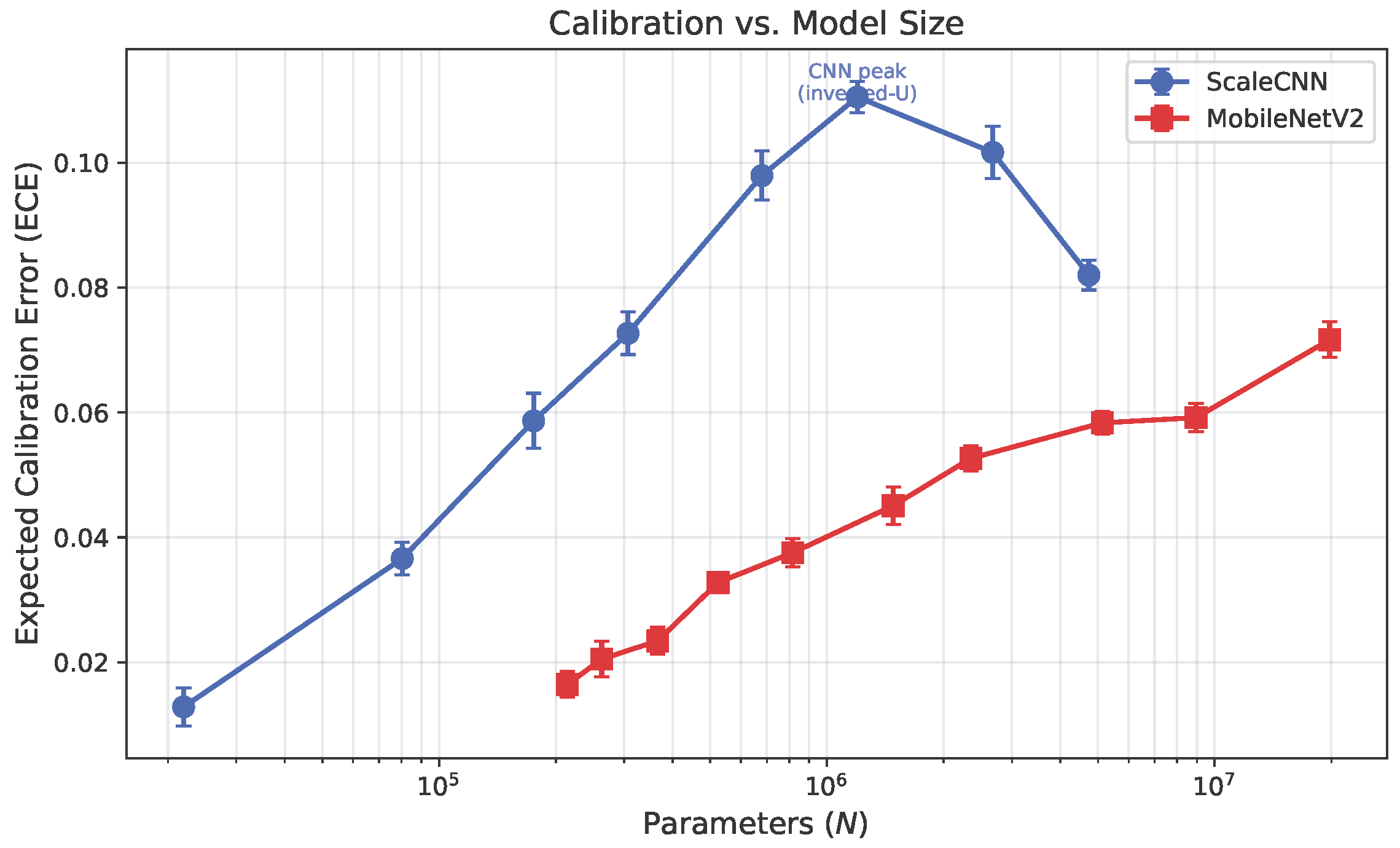
Figure 8 presents the relationship between ECE and model size.

Figure 8. Expected Calibration Error (ECE) vs. model size. ScaleCNN shows an inverted-U pattern with peak miscalibration at $c=32$ (1.2 M params). MobileNetV2 shows monotonically increasing ECE with a jump at the saturated $m=3.0$. The smallest models in both families register the lowest ECE values, although this partly reflects a global-mean matching artifact (Section 5.6).

The two architectures show different calibration trajectories:

• ScaleCNN: An inverted-U pattern. ECE rises from 0.013 ($c=4$) to a peak of 0.110 ($c=32$, 1.2 M parameters), then recovers to 0.082 ($c=64$, 4.7 M parameters). Mid-sized models are the most miscalibrated.
• MobileNetV2: Monotonically increasing ECE from 0.016 ($m=0.10$) to 0.072 ($m=3.0$). At the saturated $m=3.0$ endpoint, ECE jumps upward even though accuracy barely changes; the model grows more overconfident without becoming more capable (cf. Section 5.3).

Despite their low accuracy, the smallest models register the lowest ECE values in both families. A 22 K-parameter ScaleCNN with 42% accuracy (ECE = 0.013) yields a numerically lower calibration error than a 1.2 M-parameter model with 72% accuracy (ECE = 0.110). However, this advantage is partly an artifact of global-mean matching: small models produce near-uniform confidence distributions concentrated close to the average accuracy, which lowers ECE without implying well-calibrated per-bin estimates. With this caveat in mind, confidence scores from very small models may still be useful for rejection or deferral decisions in practice, but a low ECE alone should not be interpreted as evidence of fine-grained calibration in this regime.

6. Discussion

6.1. Reconciling Theory and Measurement

The spectral capacity theory (Section 3) correctly predicts the functional form and qualitative architecture dependence of the scaling exponent. Direct measurement of the CIFAR-100 eigenspectrum yields ${\beta }_{\mathrm{CIFAR}}=1.45$ ($R^2=0.996$), resolving the 2–3× gap that appeared when using literature estimates for natural images at native resolution ($\beta \approx 1.1$). With the measured $\beta$, the back-calculated rank efficiency exponents (${\gamma }_{\mathrm{CNN}}=0.35$, ${\gamma }_{\mathrm{MobNet}}=0.24$) are physically plausible: both are below the theoretical bound of $\gamma =0.5$, and the ordering reflects the greater structural overhead of MobileNetV2’s depthwise separable design. The remaining open question is whether $\gamma$ can be measured independently from the stable rank of intermediate activations; doing so would make the spectral capacity framework fully predictive.

6.2. Architecture Dependence

For very small parameter budgets (<500 K), our data suggest that plain convolutional architectures outperform efficient designs like MobileNetV2. The 47% exponent gap (${\alpha }_{\mathrm{CNN}}=0.156$ vs. ${\alpha }_{\mathrm{MobNet}}=0.106$) reflects structural overhead: MobileNetV2’s depthwise separable layers, 1 × 1 bottleneck projections, and expansion layers consume parameters without proportionally increasing representational capacity at small widths. This overhead washes out at large widths (MobileNetV2 was designed for efficient inference on ImageNet-scale models) but becomes a significant capacity penalty in the sub-1 M regime. Practitioners targeting microcontroller deployment may be better served by plain convolutions, reserving inference-optimized architectures for budgets where their computational efficiency advantage outweighs the capacity cost.

6.3. Implications for Edge Deployment

A common approach in edge deployment is to train a large model, compress it, verify that aggregate accuracy remains acceptable, and deploy. Our error redistribution results suggest this workflow is insufficient. With Jaccard overlap as low as 0.35 between the smallest and largest models, the error behavior of a large model is not predictive of which inputs the compressed model will misclassify. Validation must therefore occur at the target deployment size.

The cross-architecture Jaccard data reinforce this point: at matched parameter counts, a different architecture predicts deployment-time failure modes better than the same architecture at a larger size. The MobileNetV2 saturation data add a related caution: scaling beyond $m=1.5$ on CIFAR-100 yields negligible accuracy gains while increasing ECE, so model capacity should be matched to dataset size.

6.4. Class-Level Disparities Under Capacity Constraints

Compression imposes a measurable cost on class-level fairness. At 22 K parameters, the per-class accuracy Gini is 0.257, meaning a substantial fraction of classes are largely neglected. As the model grows to 4.7 M parameters, the Gini drops to 0.087, and accuracy gains flow disproportionately to the hardest classes.

The concern is sharpest in domains where rare classes carry outsized importance, such as uncommon conditions in medical imaging or unusual road scenarios in autonomous driving. Our data shows that small models degrade most on exactly these categories. This is expected: SGD on cross-entropy loss allocates capacity roughly in proportion to class frequency, so rare classes are learned last and forgotten first under capacity constraints.

7. Limitations

The clearest limitation is scope: all results come from a single dataset (CIFAR-100, 32 × 32, 50 K training images, 100 balanced classes) and two architectures. The largest model has a parameter-to-sample ratio of 396:1, so the upper end of our range is partially a study of overfitting rather than pure capacity scaling. The TinyML architecture zoo is much larger than what we test (binary networks, NAS-derived architectures, and tiny vision transformers may behave differently), and our findings may not transfer to higher-resolution datasets or other modalities like audio.

A related concern is that we scale by width only. Depth is held fixed (4 blocks for ScaleCNN, 17 for MobileNetV2), so parameters, FLOPs, and activation memory are perfectly correlated in our experiments. We cannot disentangle capacity effects from compute effects. On the training side, our convergence criterion (loss change <1% in the last 20 epochs) flagged most runs as not fully converged, likely an artifact of the cosine learning rate schedule. Convergence spot checks on ScaleCNN ($c\in \{4,32,64\}$) confirmed that accuracy plateaus before epoch 200. We performed analogous checks on representative MobileNetV2 configurations ($m\in \{0.10,1.00,3.00\}$): $m=0.10$ and $m=1.00$ show clear accuracy plateaus by epoch 180, while $m=3.0$ (19.8 M parameters) shows continued slow improvement in training loss through epoch 200, consistent with its massively overparameterized regime (396:1 parameter-to-sample ratio). The test accuracy for $m=3.0$ stabilizes by epoch 160 (final 40 epochs: $\Delta$accuracy $<0.1\%$), confirming that the saturation finding in Section 5.3 reflects a genuine capacity ceiling rather than an optimization artifact. The 200-epoch budget is standard for CIFAR-100, but some of the scaling behavior may reflect optimization dynamics rather than pure capacity.

The theoretical framework still has a gap: while we now measure $\beta$ directly from the CIFAR-100 eigenspectrum, $\gamma$ remains back-calculated from the measured exponents rather than measured independently. The theory–measurement reconciliation in Section 3.4 is therefore a partial validation rather than a fully independent prediction. For the error redistribution results, the Jaccard overlap of 0.35 is partly a consequence of the 33-point accuracy gap between the smallest and largest models; even with maximal subset containment, the Jaccard would be bounded near 0.58, so the effect is real but its magnitude is inflated. Finally, with only 8 (ScaleCNN) and 10 (MobileNetV2) data points, we cannot rigorously discriminate between a power law and other smooth functions (log-linear, stretched exponential, BNSL). Proper model selection via AIC/BIC with denser sampling would be needed to settle the functional form.

8. Conclusions

Neural scaling laws do extend to the sub-20 M parameter regime. Across 90 runs on CIFAR-100, both ScaleCNN and MobileNetV2 follow approximate power laws with error-rate exponents of $\alpha =0.156$ and $0.106$, respectively. The scaling is not uniform: local exponents decay from 0.23 in the tiny regime toward 0.10 at the upper end, and MobileNetV2 saturates at 19.8 M parameters (${\alpha }_{\mathrm{local}}=0.006$) while ScaleCNN continues to improve.

For practitioners, the more important result is what happens to the error distribution. Reducing model size changes which inputs are misclassified: the Jaccard overlap between the smallest and largest ScaleCNN error sets is only 0.35. Small models concentrate their capacity on easy classes (Gini 0.26 → 0.09) and sacrifice the hardest ones (bottom-5 class accuracy 10% → 53%). The smallest models also achieve the lowest ECE (0.013), opposite to the expected trend, though this partly reflects a global-mean matching artifact, as these models produce near-uniform confidence distributions rather than well-calibrated per-bin estimates.

On CIFAR-100, the bottom line for edge deployment is that aggregate accuracy does not tell you enough. The error distribution of a compressed model differs qualitatively from that of a larger model, and evaluation at the actual deployment size is essential. These findings are based on a single dataset (CIFAR-100) and two architectures; whether the specific exponents and redistribution patterns generalize to other datasets, resolutions, and model families is an open question that we highlight as the most important direction for future work.

9. Future Work

The most obvious gap in this study is dataset coverage. CIFAR-10 (fewer classes), Tiny ImageNet (200 classes, 64 × 64, more training data), and Speech Commands v2 (audio, a standard TinyML benchmark) would test whether the scaling exponents and error redistribution patterns we observe are specific to CIFAR-100 or reflect something more general about the small-model regime. Extending to EfficientNet-Lite, tiny vision transformers, and NAS-derived architectures would clarify whether the architecture-dependence finding holds broadly. With denser sampling of model sizes, it would also be possible to do proper model selection (AIC/BIC) to distinguish between a power law, a broken power law, and other candidate functional forms.

It is also worth testing whether error redistribution generalizes beyond width scaling. Applying structured pruning and post-training quantization to the trained models from this study would reveal whether all forms of capacity reduction produce the same kind of error rearrangement, or whether width scaling is a special case. Evaluating the same models on CIFAR-100-C [31] would test whether robustness degrades smoothly or shows sharper collapses at particular model sizes.

The remaining theoretical gap is measuring $\gamma$ independently from the effective rank of trained networks, which would make the spectral capacity framework fully predictive. On the applied side, measuring inference latency, energy, and peak RAM on Cortex-M4/M7 hardware would connect scaling behavior to the deployment metrics that practitioners actually optimize for.

References

- Kaplan, J.; McCandlish, S.; Henighan, T.; Brown, T.B.; Chess, B.; Child, R.; Gray, S.; Radford, A.; Wu, J.; Amodei, D. Scaling Laws for Neural Language Models. arXiv 2020, arXiv:2001.08361. [Google Scholar] [CrossRef] [Scilit]
- Hoffmann, J.; Borgeaud, S.; Mensch, A.; Buchatskaya, E.; Cai, T.; Rutherford, E.; Casas, D.d.L.; Hendricks, L.A.; Welbl, J.; Clark, A.; et al. Training Compute-Optimal Large Language Models. Adv. Neural Inf. Process. Syst. 2022, 35, 30016–30030. [Google Scholar]
- Zhai, X.; Kolesnikov, A.; Houlsby, N.; Beyer, L. Scaling Vision Transformers. In Proceedings of the IEEE/CVF Conference on Computer Vision and Pattern Recognition, New Orleans, LA, USA, 18–24 June 2022; pp. 12104–12113. [Google Scholar]
- Clark, A.; de Las Casas, D.; Guy, A.; Mensch, A.; Paganini, M.; Hoffmann, J.; Damoc, B.; Hechtman, B.A.; Cai, T.; Borgeaud, S.; et al. Unified Scaling Laws for Routed Language Models. In Proceedings of the 39th International Conference on Machine Learning, Baltimore, MD, USA, 17–23 July 2022; PMLR: Cambridge, MA, USA, 2022; Volume 162, pp. 4057–4086. [Google Scholar]
- Hestness, J.; Narang, S.; Ardalani, N.; Diamos, G.; Jun, H.; Kianinejad, H.; Patwary, M.M.A.; Yang, Y.; Zhou, Y. Deep Learning Scaling is Predictable, Empirically. arXiv 2017, arXiv:1712.00409. [Google Scholar] [CrossRef] [Scilit]
- Sharma, U.; Kaplan, J. Scaling Laws from the Data Manifold Dimension. J. Mach. Learn. Res. 2022, 23, 343–376. [Google Scholar]
- Bahri, Y.; Dyer, E.; Kaplan, J.; Lee, J.; Sharma, U. Explaining Neural Scaling Laws. Proc. Natl. Acad. Sci. USA 2024, 121, e2311878121. [Google Scholar] [CrossRef] [Scilit] [PubMed]
- Rosenfeld, J.S.; Rosenfeld, A.; Belinkov, Y.; Shavit, N. A Constructive Prediction of the Generalization Error Across Scales. In Proceedings of the International Conference on Learning Representations, Addis Ababa, Ethiopia, 26–30 April 2020. [Google Scholar]
- Nakkiran, P.; Kaplun, G.; Bansal, Y.; Yang, T.; Barak, B.; Sutskever, I. Deep Double Descent: Where Bigger Models and More Data Can Hurt. J. Stat. Mech. Theory Exp. 2021, 2021, 124003. [Google Scholar] [CrossRef] [Scilit]
- Caballero, E.; Gupta, K.; Rish, I.; Krueger, D. Broken Neural Scaling Laws. In Proceedings of the International Conference on Learning Representations, Kigali, Rwanda, 1–5 May 2023. [Google Scholar]
- Hinton, G.; Vinyals, O.; Dean, J. Distilling the Knowledge in a Neural Network. arXiv 2015, arXiv:1503.02531. [Google Scholar] [CrossRef] [Scilit]
- Li, H.; Kadav, A.; Durdanovic, I.; Samet, H.; Graf, H.P. Pruning Filters for Efficient ConvNets. In Proceedings of the International Conference on Learning Representations, Toulon, France, 24–26 April 2017. [Google Scholar]
- Jacob, B.; Kligys, S.; Chen, B.; Zhu, M.; Tang, M.; Howard, A.; Adam, H.; Kalenichenko, D. Quantization and Training of Neural Networks for Efficient Integer-Arithmetic-Only Inference. In Proceedings of the IEEE/CVF Conference on Computer Vision and Pattern Recognition, Salt Lake City, UT, USA, 18–23 June 2018; pp. 2704–2713. [Google Scholar]
- Lin, J.; Chen, W.M.; Lin, Y.; Cohn, J.; Gan, C.; Han, S. MCUNet: Tiny Deep Learning on IoT Devices. In Proceedings of the Advances in Neural Information Processing Systems, Virtual, 6–12 December 2020; Curran Associates, Inc.: Red Hook, NY, USA, 2020; Volume 33, pp. 11711–11722. [Google Scholar]
- Banbury, C.; Zhou, C.; Fedorov, I.; Navarro, R.M.; Thakker, U.; Gope, D.; Reddi, V.J.; Mattina, M.; Whatmough, P.N. MicroNets: Neural Network Architectures for Deploying TinyML Applications on Commodity Microcontrollers. Proc. Mach. Learn. Syst. 2021, 3, 517–532. [Google Scholar]
- Banbury, C.; Reddi, V.J.; Torelli, P.; Holleman, J.; Jeffries, N.; Kirber, C.; Montino, P.; Kanter, D.; Ahmed, S.; Philipose, M.; et al. MLPerf Tiny Benchmark. Adv. Neural Inf. Process. Syst. 2021, 34, 21097–21110. [Google Scholar]
- Lin, J.; Zhu, L.; Chen, W.M.; Wang, W.C.; Gan, C.; Han, S. On-Device Training Under 256KB Memory. In Proceedings of the Advances in Neural Information Processing Systems, New Orleans, LA, USA, 28 November–9 December 2022; Curran Associates, Inc.: Red Hook, NY, USA, 2022; Volume 35, pp. 22941–22954. [Google Scholar]
- Ray, P.P. A Review on TinyML: State-of-the-Art and Prospects. J. King Saud Univ.-Comput. Inf. Sci. 2022, 34, 1595–1623. [Google Scholar] [CrossRef] [Scilit]
- Warden, P.; Situnayake, D. TinyML: Machine Learning with TensorFlow Lite on Arduino and Ultra-Low-Power Microcontrollers; O’Reilly Media: Sebastopol, CA, USA, 2019. [Google Scholar]
- Liberis, E.; Lane, N.D. Differentiable Neural Network Pruning to Enable Smart Applications on Microcontrollers. In Proceedings of the ACM on Interactive, Mobile, Wearable and Ubiquitous Technologies; Association for Computing Machinery: New York, NY, USA, 2023; Volume 6, pp. 1–19. [Google Scholar] [CrossRef] [Scilit]
- Wei, J.; Tay, Y.; Bommasani, R.; Raffel, C.; Zoph, B.; Borgeaud, S.; Yogatama, D.; Bosma, M.; Zhou, D.; Metzler, D.; et al. Emergent Abilities of Large Language Models. Trans. Mach. Learn. Res. 2022. Available online: https://openreview.net/forum?id=yzkSU5zdwD (accessed on 10 April 2026).
- Schaeffer, R.; Miranda, B.; Koyejo, S. Are Emergent Abilities of Large Language Models a Mirage? Adv. Neural Inf. Process. Syst. 2023, 36, 2425. [Google Scholar]
- Hooker, S.; Moorosi, N.; Clark, G.; Bengio, S.; Denton, E. Characterising Bias in Compressed Models. arXiv 2020, arXiv:2010.03058. [Google Scholar] [CrossRef] [Scilit]
- Liebenwein, L.; Baykal, C.; Carter, B.; Gifford, D.; Rus, D. Lost in Pruning: The Effects of Pruning Neural Networks beyond Test Accuracy. Proc. Mach. Learn. Syst. 2021, 3, 589–602. [Google Scholar]
- Guo, C.; Pleiss, G.; Sun, Y.; Weinberger, K.Q. On Calibration of Modern Neural Networks. In Proceedings of the International Conference on Machine Learning, Sydney, Australia, 6–11 August 2017; PMLR: Cambridge, MA, USA, 2017; Volume 70, pp. 1321–1330. [Google Scholar]
- Alabdulmohsin, I.M.; Neyshabur, B.; Zhai, X. Revisiting Neural Scaling Laws in Language and Vision. In Proceedings of the Advances in Neural Information Processing Systems, New Orleans, LA, USA, 28 November–9 December 2022; Curran Associates, Inc.: Red Hook, NY, USA, 2022; Volume 35, pp. 22300–22312. [Google Scholar]
- Ruderman, D.L. The Statistics of Natural Images. Netw. Comput. Neural Syst. 1994, 5, 517–548. [Google Scholar] [CrossRef]
- Hyvärinen, A.; Hurri, J.; Hoyer, P.O. Natural Image Statistics: A Probabilistic Approach to Early Computational Vision; Springer: Berlin/Heidelberg, Germany, 2009. [Google Scholar]
- Sandler, M.; Howard, A.; Zhu, M.; Zhmoginov, A.; Chen, L.C. MobileNetV2: Inverted Residuals and Linear Bottlenecks. In Proceedings of the IEEE/CVF Conference on Computer Vision and Pattern Recognition, Salt Lake City, UT, USA, 18–23 June 2018; pp. 4510–4520. [Google Scholar]
- DeVries, T.; Taylor, G.W. Improved Regularization of Convolutional Neural Networks with Cutout. arXiv 2017, arXiv:1708.04552. [Google Scholar] [CrossRef] [Scilit]
- Hendrycks, D.; Dietterich, T. Benchmarking Neural Network Robustness to Common Corruptions and Perturbations. In Proceedings of the International Conference on Learning Representations, New Orleans, LA, USA, 6–9 May 2019. [Google Scholar]
Disclaimer/Publisher’s Note: The statements, opinions and data contained in all publications are solely those of the individual author(s) and contributor(s) and not of MDPI and/or the editor(s). MDPI and/or the editor(s) disclaim responsibility for any injury to people or property resulting from any ideas, methods, instructions or products referred to in the content. |
© 2026 by the authors. Licensee MDPI, Basel, Switzerland. This article is an open access article distributed under the terms and conditions of the Creative Commons Attribution (CC BY) license.