


Abstract
Understanding Alzheimer’s Disease (AD) progression using resting-state functional Magnetic Resonance Imaging (rs-fMRI) remains an open challenge. Variational Autoencoders (VAEs) provide compact representations of high-dimensional neuroimaging data but lack mechanisms to highlight disease-relevant features. We propose KS-VAE, a novel framework that integrates the Kolmogorov–Smirnov test into the latent space of VAEs to identify statistically significant variables discriminating healthy from pathological brain states. This integration enables measurement of latent space shifts associated with cognitive decline, offering a quantitative approach to neurodegenerative processes. By modifying the most relevant variables, KS-VAE generates synthetic samples that simulate transitions between clinical conditions while preserving anatomical plausibility. The method enhances the modeling of temporal and distributional dynamics underlying disease progression and provides interpretable analysis of class-relevant features. Applied to rs-fMRI scans of 220 subjects from the ADNI cohort, KS-VAE demonstrated robust class separation between cognitively normal and Alzheimer’s disease subjects, achieving a classification accuracy of 84.5% and an F1-score of 84.5%, and clinically consistent synthetic transitions. KS-VAE thus offers a statistically grounded and clinically interpretable framework for understanding Alzheimer’s disease progression.
1. Introduction
Alzheimer’s disease (AD) is the most common cause of dementia and has become a global health problem with enormous individual and societal implications. It is estimated that by 2050, the prevalence of dementia will double in Europe and triple worldwide [1]. Currently, around 44 million people live with dementia, and this figure could exceed 150 million in the coming decades due to population aging [2]. AD is one of the leading causes of mortality and disability in older people, with significant socioeconomic impact on healthcare systems and the families of patients [2].
Despite advances in understanding the disease’s pathogenesis since its first description by Alois Alzheimer in 1907, no disease-modifying treatments capable of slowing its progression currently exist [3]. This fact highlights the urgent need to develop new therapeutic strategies aimed not only at managing symptoms but also at preventing and treating the disease in its earliest stages.
Variational Autoencoders (VAEs) have emerged as a powerful tool in deep learning for modeling latent representations of complex biomedical data [4]. In biomedical informatics, VAEs and related architectures have been applied to tasks such as molecule design, multi-omics data integration, and medical image analysis [4,5]. In the neuroimaging domain, convolutional autoencoder models have been employed to capture hierarchical features of brain activity from functional Magnetic Resonance Imaging (fMRI) data [6], while latent generative models have been used to synthesize medical images for data augmentation in classification and segmentation tasks [7], perform disease classification, integrate heterogeneous imaging data, and capture longitudinal brain patterns [8]. More specifically, VAEs have been applied to model ageing trajectories in imaging data [9,10], integrate imaging and clinical data to better understand Parkinson’s progression [11], and harmonize data acquired from different scanners [12]. While these advances demonstrate the ability of VAEs to extract meaningful representations and generate plausible synthetic data, they do not explicitly identify disease-relevant variables in the latent space.
Previous generative frameworks, such as Attri-VAE, aim to improve the interpretability of latent representations to facilitate the generation of synthetic disease trajectories, but they generally rely on architectural constraints or regularization techniques to highlight relevant features [13]. In contrast, our KS-VAE framework integrates statistical testing into latent representation learning, enabling principled detection of features that discriminate healthy and pathological brain states.
Beyond their ability to compress high-dimensional neuroimaging data, VAEs allow the controlled generation of synthetic samples by manipulating latent variables associated with clinical status. This capability makes them particularly suited for simulating disease progression, generating intermediate representations, and exploring how specific latent dimensions relate to cognitive decline [14].
This work introduces KS-VAE, a framework that explores the latent space of a VAE trained in an unsupervised manner on resting-state functional Magnetic Resonance Imaging (rs-fMRI) brain images. To quantify the transformation from healthy to pathological brain activity, the Kolmogorov–Smirnov (K-S) test is applied to each latent coordinate as a post hoc analysis tool to identify dimensions whose distributions differ significantly between cognitively normal (CN) and Alzheimer’s disease (AD) subjects. These statistically relevant coordinates are then used to guide controlled latent manipulations that generate synthetic transitions between clinical conditions. Finally, the modified latent representations are decoded back into synthetic brain volumes. This approach allows the analysis of disease-related changes in functional connectivity patterns, supporting interpretable modeling of neurodegenerative progression and controlled generation of synthetic neuroimaging data.
The novelty of the proposed KS-VAE framework lies in the integration of statistical hypothesis testing with deep generative modeling in order to improve the interpretability of latent representations. While conventional variational autoencoders learn latent spaces that are often difficult to interpret, the proposed approach explicitly analyzes each latent coordinate using the Kolmogorov–Smirnov test to identify statistically significant differences between diagnostic groups. These statistically relevant dimensions are then used to guide controlled latent manipulations that simulate transitions between healthy and pathological functional patterns. This combination of statistical testing and generative modeling provides an interpretable, statistically grounded mechanism for exploring disease-related variability in neuroimaging data, beyond what is achievable with conventional VAEs.
2. Theoretical Background and Materials
2.1. Dataset:Alzheimer’s Disease Neuroimaging Initiative (ADNI)
The Alzheimer’s Disease Neuroimaging Initiative (ADNI) is one of the most recognized datasets in AD research. This database provides a wide range of brain images and associated clinical data [15,16].
ADNI is a multicenter longitudinal study designed to develop clinical, imaging, genetic, and biochemical biomarkers for early detection and monitoring of AD. Since its launch in 2004, ADNI has facilitated data collection and sharing among researchers worldwide [15,16].
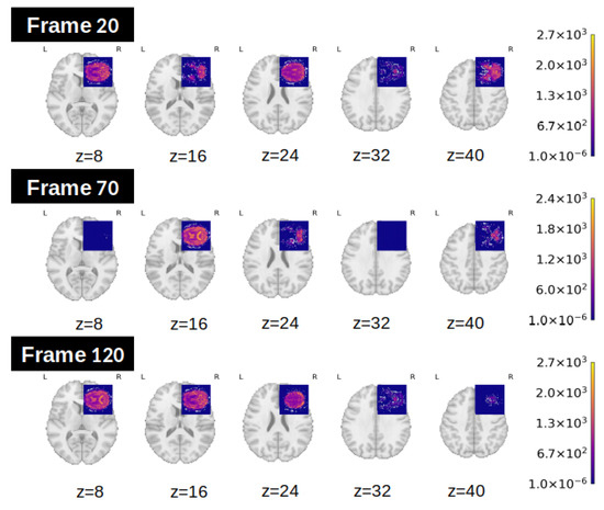
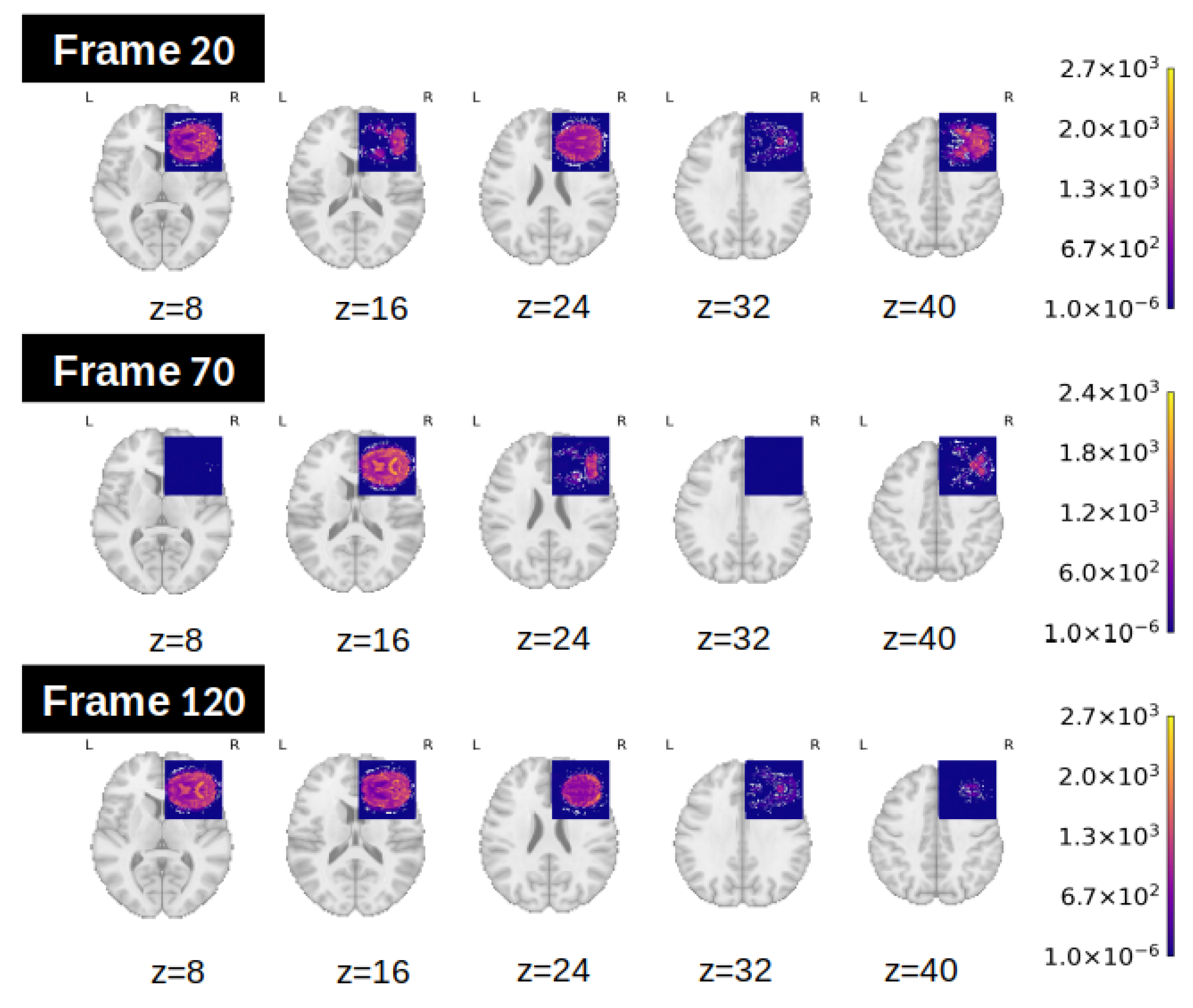
The present study focuses on the resting-state functional MRI subset of the ADNI dataset, which comprises volumetric brain images with a spatial resolution of voxels across 48 axial slices, acquired over 140 time points per subject. Each sample is thus represented as a 4D data tensor of shape . To illustrate this structure, Figure 1 shows 9 representative axial slices from a single time point of an rs-fMRI scan. Each slice corresponds to a matrix at a different position along the Z-axis, and the 48 slices together form a complete volumetric brain representation. Stacking these volumes across the 140 time points yields the full 4D input.
Figure 1.
Example of 15 axial slices ( pixels each) extracted from different time points and spatial positions in an rs-fMRI scan. Each column corresponds to a different slice along the Z-axis (depth), and each row corresponds to a different time point. A full fMRI volume at a given time consists of 48 axial slices acquired sequentially along the Z-axis. Colorbars in the corner indicate voxel intensity values, obtained by mapping raw signal intensities to colors using the plasma colormap provided in Nilearn’s plot_stat_map function [17].
Although the dataset includes subjects across a spectrum of cognitive states, this study is restricted to those clinically labeled as either cognitively normal(CN) or diagnosed with Alzheimer’s disease (AD), enabling a focused binary classification task.
2.2. Regional Homogeneity (ReHo)
Regional Homogeneity (ReHo) is a widely used metric in rs-fMRI analysis to quantify the degree of local synchronization of neural activity. It is based on the assumption that brain regions involved in the same functional network exhibit temporally coherent activity at rest [18].
Given a 4D fMRI volume , where T is the number of time points and denote the spatial dimensions, ReHo is computed voxel-wise by evaluating the temporal similarity between the time series of a given voxel and those of its spatial neighbors.
For a target voxel v located at , let denote its time series across all frames. The set of its 26 nearest neighbors in a cube (excluding v itself) is denoted by . For each neighbor , let be its corresponding time series.
ReHo was defined by Zang et al. as Kendall’s coefficient of concordance (W) among the time series of a given voxel and its neighbors [18]. Formally,
where K is the number of time series (the voxel v plus its neighbors), n is the length of each time series, and is the sum of ranks of the i-th time point across the K series.
This metric captures the consistency of the temporal patterns within a local cluster of voxels. Higher ReHo values indicate greater synchronization with neighboring voxels, which may reflect localized functional integration or pathology-induced hyper-synchronization.
2.3. Statistical Analysis: Kolmogorov–Smirnov Test
The Kolmogorov–Smirnov (K-S) test is a non-parametric statistical test used to compare the distributions of two independent samples. It assesses whether the samples come from the same continuous distribution, making no assumptions about the shape or parameters of that distribution [19].
Given two samples and , the test computes the maximum absolute difference between their empirical cumulative distribution functions (ECDFs), defined as:
where and are the ECDFs of samples X and Y, respectively. A larger value of indicates a greater discrepancy between the distributions. The test statistic is compared to a critical value to determine statistical significance.
2.4. Variational Autoencoders
Variational Autoencoders (VAEs) are generative models that learn a probabilistic mapping from data to a latent space. Unlike standard autoencoders, VAEs model the encoder as a posterior distribution and the decoder as a likelihood , with a prior on the latent variables.
The objective is to maximize the Evidence Lower Bound (ELBO):
where the first term encourages accurate reconstruction and the second regularizes the posterior distribution, ensuring it stays close to the prior . This way, the KL-divergence term prevents the model from overfitting to individual training samples and provides the latent space needed for good generalization and for generating new samples.
A common way to monitor VAE training performance is through the average reconstruction loss, defined as the mean value of the reconstruction term across the training set.
3. Methodology
This section presents KS-VAE, the novel methodological framework developed in this study to analyze and understand the progression of cognitive impairment. KS-VAE extends the standard use of VAEs by integrating the K-S test into the analysis of the latent space, enabling principled identification of disease-relevant dimensions. This integration allows the generation of synthetic brain images that simulate controlled transitions between clinical conditions, thereby enhancing the interpretability of cognitive trajectories.
To construct KS-VAE, multiple VAEs are first trained in an unsupervised manner on high-dimensional rs-fMRI brain volumes, without incorporating temporal ordering during training. This strategy enables the exploration of different latent space dimensionalities, from which the configuration with optimal reconstruction fidelity was selected. Once the optimal latent space is obtained, its utility is preliminarily evaluated using standard machine learning classifiers, which assess whether the embeddings encode discriminative information between CN and AD subjects. This step ensures the relevance of the learned representations before proceeding to more advanced analyses.
The K-S test is then applied within the KS-VAE framework to identify the most discriminative latent dimensions. For each dimension, the ECDFs of CN and AD subjects are compared, providing a statistically principled measure of global distribution differences, rather than focusing solely on means or variances or assuming any specific form. In this way, the test robustly highlights dimensions that encode clinically meaningful variability in potentially non-Gaussian latent representations. Dimensions that exhibit statistically significant differences between both groups are then selected as disease-relevant variables.
Following the application of the K-S test, synthetic samples are generated by systematically modifying the identified embeddings. This manipulation is designed to reflect a gradual progression between clinical conditions, such as from CN to AD. By controlling the transitions in this way, the framework facilitates the generation of intermediate synthetic samples, which can be visualized to understand the underlying dynamics of cognitive decline. Finally, the generated synthetic samples are validated using quantitative approaches.
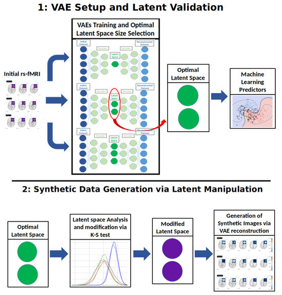
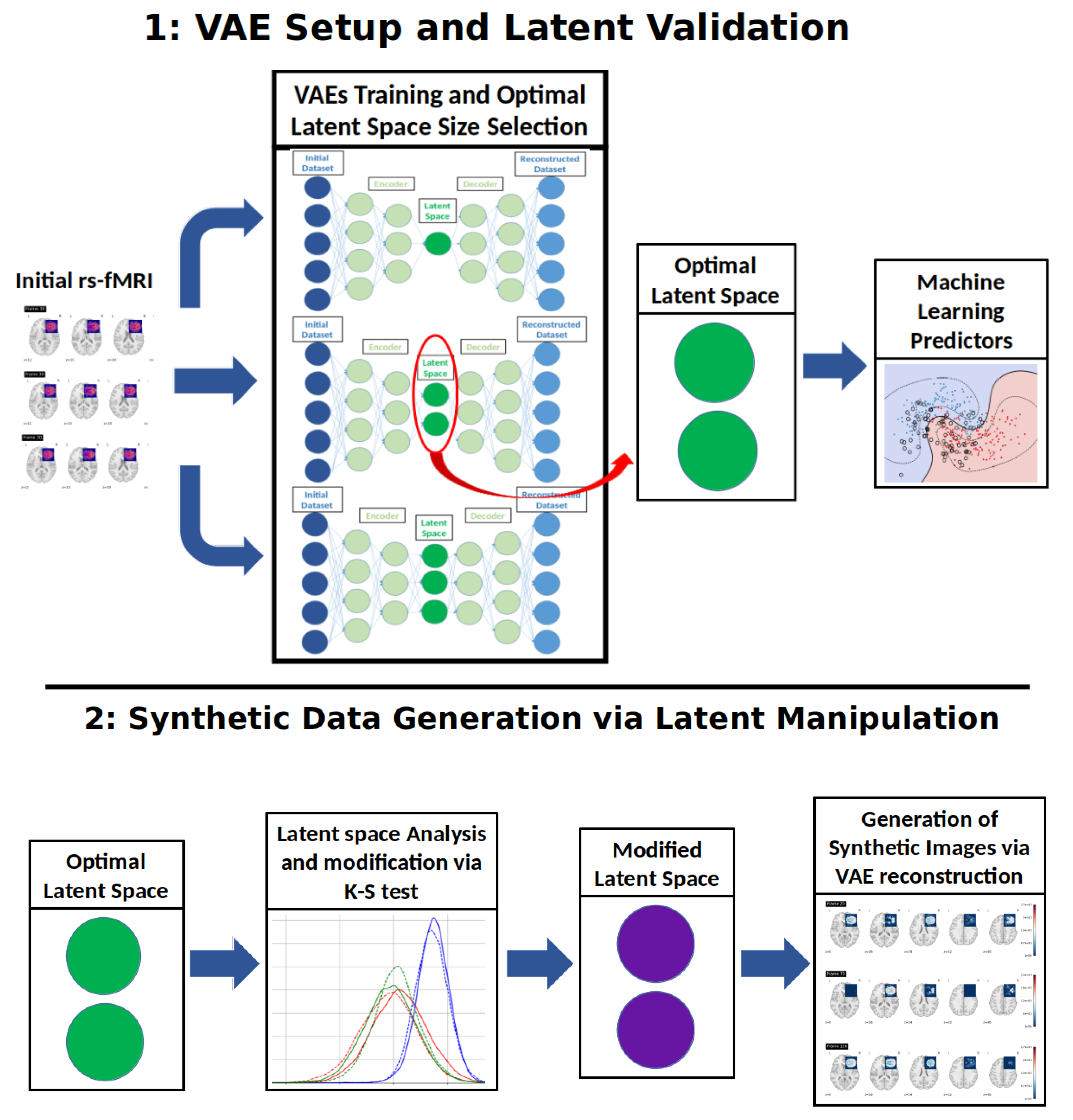
An overview of the complete methodological workflow is provided in Figure 2.
Figure 2.
Workflow of the methodology.
3.1. VAE Setup and Latent Validation
This subsection describes the construction of the VAE and the evaluation of its latent space. The evaluation is carried out using Machine Learning (ML) classifiers, with the goal of verifying that the learned representations preserve structural and class-discriminative information to support subsequent analytical tasks.
3.1.1. VAE Construction and Latent Space Extraction
The first stage of the methodology involves training a VAE to compress high-dimensional fMRI brain volumes into a lower-dimensional latent space while preserving essential anatomical information. Each input sample corresponds to a 3D resting-state fMRI volume, treated independently of its temporal context.
where the spatial dimensions of the brain volume is a vector in , and the latent space is a vector in . The encoder outputs a set of latent parameters—mean and log-variance—which define the approximate posterior distribution for each input.
The trained VAE encoder maps each temporal instance of a given input sample to a latent vector . For each sample, this yields a sequence of t latent vectors, which can be organized as , where each corresponds to the latent encoding at temporal index i. Thus, each input is ultimately represented by a sequence of t vectors in . Importantly, although each temporal frame is encoded independently by the VAE, the ordering of the latent vectors in Z matches the temporal order of the input sequence. This occurs because each latent vector is obtained by encoding the i-th temporal frame of the input and is then stored at the same index of the sequence Z, establishing a one-to-one correspondence between the input and latent sequences. During reconstruction, the decoded volumes will be reassembled in this same order, thereby preserving sufficient temporal consistency with the original data to allow downstream temporal analyses.
Latent embeddings are sampled using the reparameterization trick [20] and passed to the decoder, which attempts to reconstruct the original brain volume. The model is trained by maximizing the ELBO, defined in Equation (3).
This procedure is repeated for different values of the latent dimensionality n, allowing the selection of a compact representation that preserves sufficient information for a faithful reconstruction while avoiding an excessive large latent space that could lead to memorization of training data. The strategy for selecting n is to analyze the reconstruction loss across several candidate values and apply an elbow criterion. The optimal latent dimension is defined as the smallest element of the candidate set
satisfying the inequality
where denotes the reconstruction loss for latent dimension , is a threshold controlling the acceptable rate of diminishing returns, and the indices follow the ordering . The resulting latent vectors are retained for downstream analysis.
3.1.2. Classification Using Latent Representations
To investigate the discriminative capacity of the previously obtained latent space, we train supervised ML classifiers on the latent vectors corresponding to labeled samples. The classifiers proposed for this study include Support Vector Machines (SVM), Random Forests (RF), and eXtreme Gradient Boosting (XGBoost) [21], although the methodology is readily extensible to other models or ensemble methods.
To incorporate the temporal structure into the classification process, multiple strategies are explored:
- Mean Aggregation: Averaging the latent vectors across time to produce a single vector per subject.
- Vector Concatenation: Concatenating the full temporal sequence into a single high-dimensional vector.
- Independent Time Points: Training a separate classifier for each temporal index, and using majority voting across all frames to obtain a single prediction per subject.
Classifier training follows standard procedures, and performance is evaluated using common metrics such as accuracy and F1 score [21]. All evaluations are performed using cross-validation to ensure robust and reliable estimates.
3.2. Synthetic Data Generation via Latent Manipulation
This stage is devoted to simulating class transitions via targeted manipulations of the latent space learned by the VAE. After verifying the discriminative structure of the latent space, we explore its generative potential by synthesizing new samples that simulate a transition from one class to another. This could be achieved through a targeted modification of selected latent variables. The following describes the procedure used to generate a synthetic representation that mimics a sample transitioning from a source class to a target class .
Given a latent sequence , accounting for the temporal structure of the data, we apply a K-S test (Section 2.3) independently to each coordinate of each , comparing samples from and . This coordinate-wise test is performed separately for each time index i, i.e., the distributions of in are only compared with those of the same coordinate j and time index i.
The K-S test was selected because it provides a non-parametric way to compare the full empirical distributions of two samples without assuming any specific parametric form. This property is particularly relevant in latent spaces learned by deep generative models, where the marginal distributions of latent coordinates may deviate from simple Gaussian assumptions due to reconstruction constraints and data heterogeneity. Through the coordinate-wise comparison described above, the test allows us to capture localized, time-dependent shifts in the latent space that are informative for class discrimination.
For a latent sequence originally associated with a source class , the objective is to generate a modified sequence that preserves the temporal structure of the original while incorporating features representative of the target class .
Let be a proportion parameter, with n denoting the total number of latent variables. We select the top latent variables (denoted ) with the lowest p-values in the K-S test. For each selected coordinate , its value is replaced by the empirical mean of that coordinate in the target class, i.e., , where denotes the class-wise mean of coordinate across all samples in . Although using the average value reduces individual variability in the modified dimensions, the selected approach captures the global trend of the disease while modeling a controlled and statistically meaningful shift between clinical conditions, thereby enabling a principled examination of disease progression at the population level.
To maintain structural coherence, each modified coordinate is accompanied by changes in a subset of latent variables that are highly correlated with it. Specifically, for each , we compute its Pearson correlation with all other coordinates and select the top most correlated ones, denoted , where controls the extent of correlation propagation. These additional variables are also replaced by their respective class-wise means from the target distribution.
The parameters explicitly chosen by the user are the previously defined , which determines the number of directly modified coordinates, and , which sets an upper bound on the total fraction of latent variables allowed to change. The value of is then derived from these to ensure that the total number of modified variables remains bounded. In the worst-case scenario—where all correlation sets are disjoint—the total number of modified variables may reach . To guarantee that no more than a fraction of the latent space is altered, we impose the constraint:
We therefore set , the largest value that satisfies the constraint, in order to maximize the number of correlated variables considered per modified coordinate.
This guarantees that, even in the absence of correlation overlaps, no more than latent variables are modified. In practice, the actual number is typically lower due to overlapping correlation sets across different .
The resulting latent vectors are then passed through the decoder to generate a synthetic sample that resembles the original input structurally, but exhibits statistical characteristics of the target class.
In summary, the workflow for generating synthetic samples can be described in three main steps. First, the latent representation of each rs-fMRI volume is obtained using the encoder of the trained VAE. Second, the Kolmogorov–Smirnov test is applied independently to each latent coordinate in order to identify dimensions whose statistical distributions differ significantly between the CN and AD groups. The coordinates with the highest statistical significance (top ) are then selected as disease-relevant latent factors. Third, synthetic transitions are produced by replacing the values of these selected coordinates with the empirical mean values of the target class while leaving the remaining latent dimensions unchanged. The modified latent vectors are subsequently decoded through the VAE decoder to obtain reconstructed brain volumes that represent controlled transitions toward the target condition. This strategy allows the generation of interpretable synthetic samples that reflect statistically guided modifications in the latent space.
3.3. Evaluating Transitions with Real Patient Progression
Once synthetic data are obtained a last stage is required to evaluate the transformations introduced into the data. Two possible approaches are included in this method:
3.3.1. Assessing Synthetic Transitions Against Patient Transitions
We assess whether latent manipulations produce synthetic transitions that approximate real subject progression. For a subject with a documented worsening over time, we compare reconstructions and synthetic samples at different stages:
- : Real input at the initial stage;
- : Real input of the same patient at the later stage;
- : VAE reconstruction of ;
- : Synthetic sample obtained by manipulating the latent representation of toward the target class (Section 3.2).
We quantify discrepancies using binary cross-entropy (BCE) [22]:
A lower compared to indicates that the synthetic sample approximates the later-stage scan more closely than the simple reconstruction.
3.3.2. Assessing Synthetic Transitions Against Class-Level ReHo Patterns
To complement patient-specific comparisons, we also evaluate synthetic transitions against lass-levelReHo maps, which serve as reference connectivity patterns for each group. This approach reduces the impact of individual variability and provides a population-level benchmark. Specifically, we first reconstruct the full 4D fMRI volumes from the latent space using the trained VAE decoder, compute voxel-wise ReHo maps for each subject, and average them across all individuals belonging to the same class. This yields the reference templates
where and denote the number of subjects in each group.
Each synthetic volume is then processed in the same way to obtain its ReHo map , which is compared against the class-level benchmarks. We compute the voxel-wise distances
with denoting the mean absolute difference. The synthetic sample is assigned to the closest reference pattern,
and we define as the signed difference in distance between the two group-level patterns.
4. Results
To extract compact and meaningful representations of the brain images used in this study, we implemented a VAE as described in Section 2.4. The images used in this study correspond to rs-fMRI scans from the ADNI dataset (see Section 2.1). To handle the format of the dataset, we integrated the pydicom library [23] version 3.0.1 for image access and decoding. The model was implemented in PyTorch [24] version 2.3.1.
The VAEs were trained for 50 epochs using the ELBO objective described in Section 2.4, which balances reconstruction fidelity with KL-divergence regularization to mitigate overfitting [25]. This loss formulation encourages the latent space to approximate a standard normal distribution while capturing anatomical variability in the data. To determine the appropriate representation capacity, models were evaluated across a range of latent dimensionalities. The final latent dimension was selected using the elbow criterion described in (5), which identifies the smallest dimension beyond which further increases yield only marginal reductions in reconstruction error. Each temporal frame was processed independently as a 3D volume of shape , effectively treating time points as separate inputs during training and reconstruction.
The analysis was performed on a total of 220 studies from the ADNI database: 110 diagnosed with AD and 110 CN. Within each group, 55 were male and 55 were female, ensuring balanced representation. However, sex was not used as a predictive factor in any of the models. Note that some patients contributed more than one study.
4.1. Latent Space Validation: Dimension Selection and Class Separability
Before conducting the main experiments involving latent space manipulation, we first verify that the VAE fulfills two essential criteria: (i) the selected latent dimensionality provides sufficient reconstruction fidelity, and (ii) the latent codes preserve information relevant for class separation. This validation ensures that subsequent analyses are grounded on a meaningful and structured latent space.
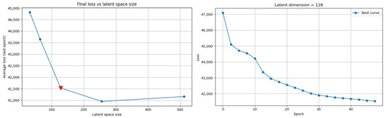
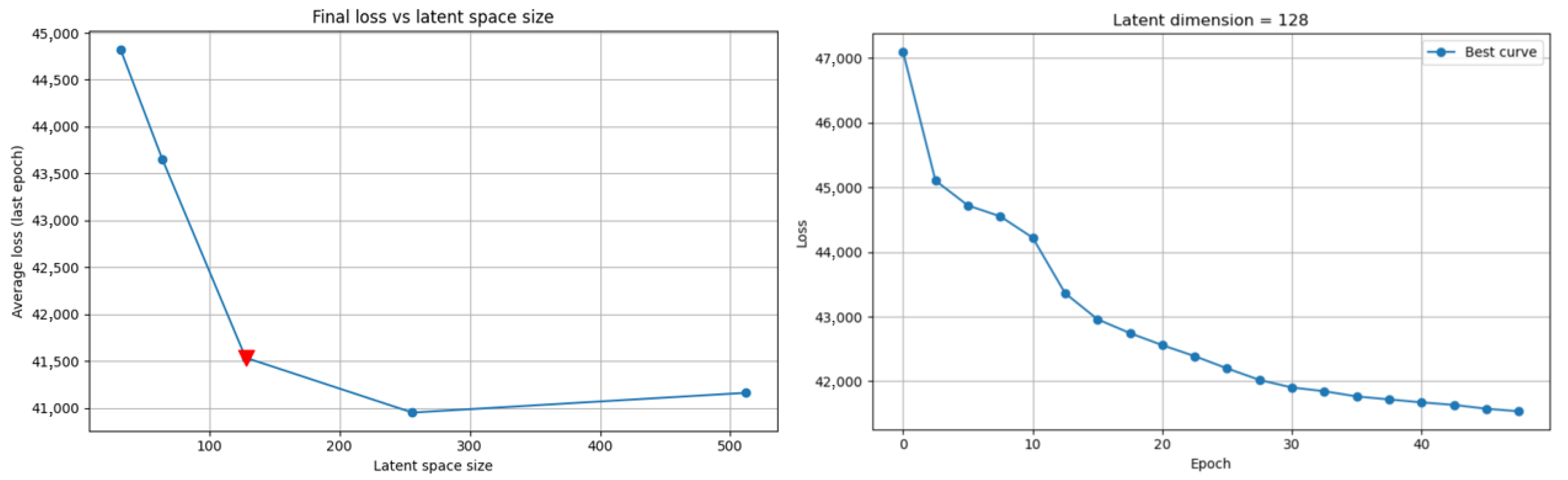
To validate the suitability of the learned latent space—constructed following the methodology described in Section 3.1.1—for downstream analysis, we first selected an optimal latent dimensionality based on reconstruction performance. Among the different configurations tested, a latent space size of 128 emerged as optimal. As shown in Figure 3, this value corresponds to an elbow in the plot of the average reconstruction loss over the final epoch, suggesting a good trade-off between model capacity and reconstruction fidelity.
Figure 3.
On the left: final average reconstruction loss for each latent space size tested, with the selected latent dimension highlighted in red. On the right: training loss per epoch for the model with a latent dimension of 128.
For latent dimension 128, the final average reconstruction loss (see Section 2.4) was approximately 41,500. Given that each input volume contains voxels, this corresponds to a relative per-voxel loss of approximately ~0.211, indicating that the VAE retains considerable spatial detail.
To assess whether the latent space captures class-discriminative information, we trained supervised classifiers using the latent representations as input features, as described in Section 3.1.2. We trained an SVM with the default regularization parameter . The RF was configured with 100 estimators and no maximum depth, while the XGBoost classifier was trained with 100 boosting rounds, a learning rate of 0.3, and maximum tree depth of 3. Performance was evaluated using 5-fold cross-validation (80% training and 20% test per fold, with a total of 220 studies), ensuring that no test labels were used during training. Although the VAE was trained on the full dataset prior to cross-validation, which might introduce a potential source of indirect information leakage, this training was done in a fully unsupervised manner and is limited to representation learning, thereby it does not involve target leakage. Table 1 reports the confusion matrices across folds for the three proposed encoding strategies: Mean Aggregation, Vector Concatenation, and Independent Time Points.
Table 1.
Flattened Confusion Matrices by Classifier and Strategy.
The best results were obtained using XGBoost with mean aggregation, achieving True Positives (TP) rates of 84% for CN and 85% for AD. This corresponds to an overall accuracy of 84.5%, precision of 84.8%, and F1-score of 84.5%. These results confirm that the latent space encodes relevant class-specific information.
4.2. Synthetic Transitions and Validation Experiments
To assess the generative capabilities and interpretability of the learned latent space, we applied the procedure detailed in Section 3.2 to generate synthetic brain representations by progressively modifying CN samples toward the AD class.
This approach leverages the K-S test to identify the most informative latent dimensions that capture disease-related variability. By selectively intervening in these dimensions, we simulate neurodegenerative trajectories within the latent space.
To this end, we performed a K-S test independently on each coordinate of the latent vectors at every time point, with corresponding to the number of temporal instances per subject. Since this step is intended as a tool to identify global distributional differences between the clinical groups at the population level for synthetic data generation, rather than predicting behaviour on unseen data, the test was applied to the complete dataset in order to maximize statistical power and generative realism. This analysis follows the procedure described in Section 3.2. Out of the 17,920 possible pairs (140 time points × 128 latent variables), a total of 2945 pairs exhibited statistically significant differences between the CN and AD groups at the level. This corresponds to 16.43% of the latent space showing meaningful class-dependent variation.
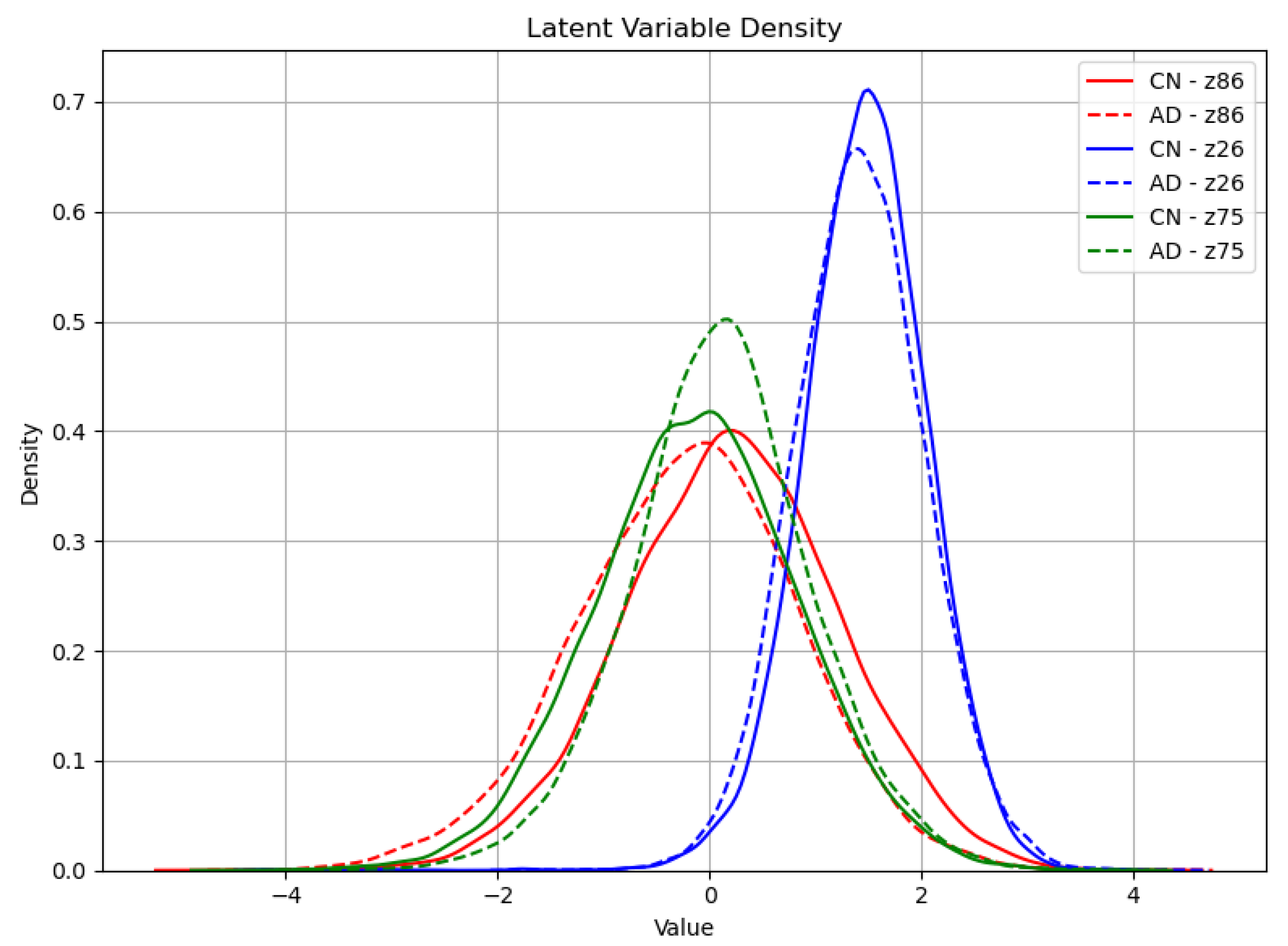
Among the most discriminative coordinates, several latent variables such as z86, z75, and z5 consistently displayed highly significant differences across multiple time points. For instance, variable z86 alone yielded p-values as low as (frame 24), and remained below in numerous other frames, indicating strong temporal consistency in its discriminative power.
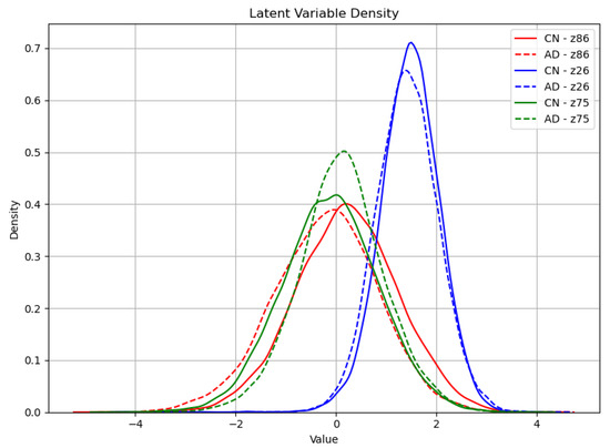
To visually contextualize these statistical findings, Figure 4 presents the empirical distributions of the three most statistically discriminative latent variables—z86, z24 and z75—stratified by diagnostic group. While the visual differences in distributional shape and central tendency between CN and AD subjects are relatively subtle and may not be immediately discernible without statistical expertise, the extremely low p-values obtained from the K-S test provide strong evidence of significant distributional divergence, thereby supporting their inclusion in the targeted modification process.
Figure 4.
Empirical distributions of latent variables z86, z24, and z75 for CN and AD subjects. These variables had the three lowest p-values in the Kolmogorov–Smirnov test.
Based on the ranked list of p-values, we selected the top coordinates—those with the strongest evidence of class difference—with . The transformation procedure outlined in Section 3.2 was then applied to these variables, using a constraint to limit the total proportion of the latent space that could be altered. Both parameters governing the KS-guided manipulation, and , were selected based on preliminary experiments, where the specified values provided a suitable trade-off between achieving a detectable class transition and maintaining fidelity to the original sample. The resulting modified latent representations were subsequently decoded into image space to visually inspect whether the class-pertinent structural patterns were reflected in the output.
4.2.1. Assessing Synthetic Transitions Against Patient Transitions
As a direct application of the methodological framework described in Section 3.3.1, we conduct a small-scale exploratory experiment to evaluate whether the synthetic latent manipulations yield clinically meaningful transitions. Specifically, we identify three patients for whom a clear progression towards AD is recorded in the dataset. For each, we compare their real temporal evolution with the result of applying the latent manipulation method described in Section 3.2, using the same parameter settings (, ) as in the main synthetic generation procedure. The resulting BCE values for the three progression cases are reported in Table 2.
Table 2.
BCE Values for the Three Progression Cases.
4.2.2. Assessing Synthetic Transitions Against Class-Level ReHo Patterns
Building on the procedure defined in Section 3.3.2, synthetic transitions were evaluated against population-level ReHo templates for CN and AD patients. This approach provides a benchmark that mitigates individual variability by comparing each synthetic volume with class-level connectivity patterns. Overall accuracy reached 66.82% (147/220).
Stratified by initial label, synthetic samples originating towards healthy subjects showed higher alignment with the healthy template 72.27% (80/110), while those derived towards AD patients reached 60.92% (67/110) alignment with the AD template.
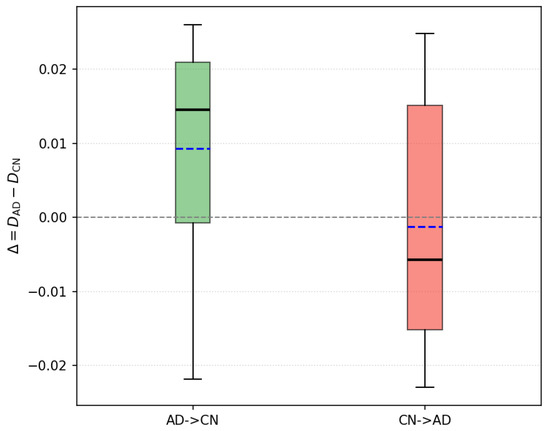
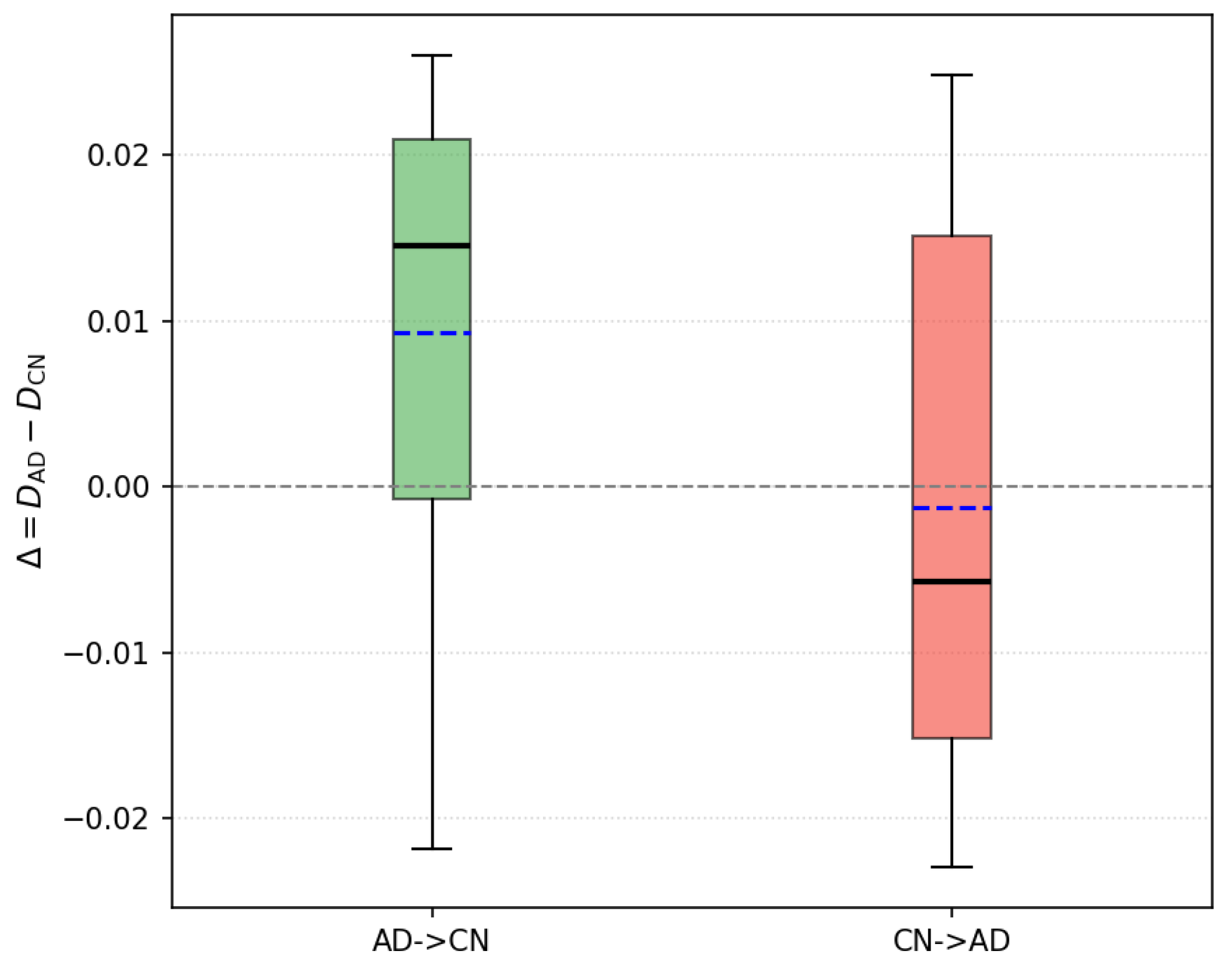
The distribution of , defined as the difference between the distances of the synthetic patient and the AD and CN ReHo templates, is shown in Figure 5. Results are stratified according to the type of transition, either AD→CN or CN→AD.
Figure 5.
Boxplot comparing group-wise distance differences across transitions. AD→CN indicates that the original condition was AD, and conversely for CN→AD. Black lines represent medians, blue lines represent means, and the grey dotted line at indicates the expected value under class-indistinguishable distributions.
5. Discussion
The results demonstrate that the latent space learned by the KS-VAE encodes clinically relevant structure, enabling controlled generation of synthetic samples. However, the current pipeline combines unsupervised encoding and synthetic manipulation without fully isolating the contribution of each. The quality of the synthetic samples ultimately depends on the latent representation produced by the encoder. Any loss of class-relevant information introduced at this stage can propagate to the generation process, compromising the ability to produce class-consistent data. Although classifiers were used to probe the structure of the latent space, the fact that the best model achieves 84.5% accuracy suggests that a non-negligible fraction of samples may already be misrepresented at the encoding level. This makes it difficult to determine whether inconsistencies in the synthetic outputs stem from the manipulation procedure or from upstream encoding errors. Addressing this issue will require strategies to better constrain or validate the latent space before generation.
Another important aspect to consider is the sensitivity of the latent manipulation procedure to the hyperparameters and described in Section 3.2. These parameters directly affect the discrepancies and described in Section 3.3.1, which quantify, respectively, the distance between the original and synthetic inputs, and the distance between the synthetic sample and the true pathological state. Increasing and tends to raise and lower , enhancing alignment with the target class but potentially distorting individual features. Lower values have the opposite effect, preserving subject-specific characteristics but weakening the class shift. Ideally, a low indicates high fidelity to the original input, while a low reflects successful alignment with the target state. Balancing these two objectives is crucial to ensure that the transformation remains both realistic and clinically meaningful.
The experiment described in Section 4.2.1 is currently conducted on a small subset of patients. Since the Kolmogorov–Smirnov test used to identify discriminative latent variables relies on empirical distribution comparisons whose sensitivity increases with the number of observations available in each group, this limited sample size may reduce statistical power and limit the number of significant identified latent coordinates. Consequently, larger datasets may reveal more discriminative latent dimensions between cognitively normal and pathological populations. Nevertheless, the variational autoencoder framework provides regularization through the KL divergence term, helping maintain stable latent representations even with moderately sized datasets. Future studies expanding it to larger longitudinal cohorts—including individuals who transition from CN to AD—could provide a more robust benchmark and yield more precise estimates of disease-related latent factors. Applying the synthetic transformation method to early-stage CN subjects and comparing the generated samples to their future AD scans would enable a more medically grounded evaluation.
The evaluation against class-level ReHo patterns (Section 4.2.2) shows that synthetic transitions capture group-level features with moderate accuracy (66.8%). The higher alignment in AD→CN than in CN→AD suggests that introducing disease-like alterations is easier than restoring healthy connectivity, likely due to the greater variability in AD patterns. The distribution of further indicates systematic differences between transition directions, highlighting the need for manipulation strategies that better account for class heterogeneity.
An additional exploratory direction involved training separate VAE models on CN and AD cohorts. Although not included in this document, this analysis suggested that models trained on distinct groups capture disease-specific variability in their latent spaces. Preliminary comparisons indicated differences between the AD-derived latent distribution and the CN latents, suggesting that separate models may capture complementary aspects of disease-specific variability. These findings highlight the potential of group-specific generative models to reveal complementary aspects of disease heterogeneity beyond what can be captured in a shared latent space.
The KS-VAE framework introduces a statistically guided approach to model the continuum between healthy and pathological brain states. By constraining latent manipulations through the Kolmogorov–Smirnov criterion, it enables the generation of clinically interpretable trajectories that mirror disease-related distributional shifts. This integration of statistical rigor and physiological relevance provides a principled foundation for understanding Alzheimer’s disease progression. The explicit incorporation of statistical testing distinguishes our approach from previous generative VAE-based methods, which rely primarily on regularization techniques to improve latent interpretability. Although the present study does not provide a quantitative comparison with these alternative approaches, such analyses would further validate the framework and constitute an important direction for future work.
Importantly, the proposed latent-space manipulation strategy is not limited to brain imaging or AD. It is trivially extensible to any dataset where inputs can be encoded via an autoencoder and are associated with two or more categorical labels, including other medical imaging modalities, time series, or even text embeddings.
From a clinical research perspective, the proposed KS-VAE framework may provide a useful tool for exploring functional brain alterations associated with Alzheimer’s disease. By identifying latent dimensions that differ significantly between cognitively normal and pathological states, the model can highlight functional patterns potentially linked to disease progression. In addition, the ability to generate controlled synthetic transitions between clinical conditions may help researchers investigate intermediate functional states that are difficult to observe directly in clinical datasets. Although the current work does not aim to provide a diagnostic system, such generative approaches may contribute to the identification of imaging biomarkers and support the design of longitudinal studies investigating early stages of neurodegeneration.
Despite these promising aspects, it should be noted that the synthetic samples generated by the KS-VAE framework are intended primarily for research exploration rather than direct clinical decision-making. While the proposed approach enables the investigation of functional transitions between clinical conditions, further validation on larger and longitudinal datasets will be necessary before such models could be considered for potential clinical applications.
Finally, it would be of interest to explore whether some latent variables consistently act as early biomarkers across individuals—i.e., variables whose distribution shifts precede clinical diagnosis. Combining this with model interpretability techniques could strengthen the method’s relevance for translational applications.
6. Conclusions
This work presented KS-VAE, a novel framework that integrates the K-S test into the latent space of a VAE trained on rs-fMRI data. By statistically identifying discriminative latent dimensions, KS-VAE enables principled measurement of shifts associated with AD progression and facilitates an interpretable analysis of class-relevant features. Furthermore, the framework allows controlled manipulation of these dimensions to generate class-consistent synthetic samples that simulate transitions between healthy and pathological states while preserving anatomical plausibility.
Beyond its direct relevance for early detection and monitoring of dementia, the method is generic, model-agnostic, and adaptable to other domains where structured input data and categorical labels are available. Future research could focus on refining the latent structure, extending evaluation to longitudinal trajectories, and exploring its potential for identifying early predictive biomarkers.
Author Contributions
Conceptualization, C.M. and C.V.; methodology, C.M. and C.V.; software, C.M.; validation, C.M. and C.V.; formal analysis, C.M. and C.V.; investigation, C.M., B.P., L.B., O.Z., J.T. and C.V.; resources, C.V.; data curation, C.M.; writing—original draft preparation, C.M., B.P., L.B., O.Z., J.T. and C.V.; writing—review and editing, C.M., B.P., L.B., O.Z., J.T. and C.V.; visualization, C.M. and C.V.; supervision, C.V.; project administration, C.V.; funding acquisition, C.V. All authors have read and agreed to the published version of the manuscript.
Funding
This work was funded and supported by the Spanish Ministry for Digital Transformation and the Civil Service (grant number TSI-100121-2024-35, project BRILLIANT), by the Spanish Ministry of Science and Innovation (grant number PID2022-138936OB-C32, project COGNISANCE), and by MCIN/AEI/10.13039/501100011033/FEDER, UE.
Informed Consent Statement
All patients are de-identified.
Data Availability Statement
The code used in this study is available from the corresponding author upon reasonable request. The datasets employed, ADNI, are publicly available to authorized users through the Laboratory of Neuro Imaging (LONI) Image and Data Archive (IDA) at https://adni.loni.usc.edu/data-samples/adni-data/ (accessed on 1 September 2025).
Conflicts of Interest
The authors declare no conflicts of interest.
Abbreviations
The following abbreviations are used in this manuscript:
| AD | Alzheimer’s disease |
| BCE | Binary cross-entropy |
| CN | Cognitively normal |
| ECDFs | Empirical cumulative distribution functions |
| ELBO | Evidence Lower Bound |
| fMRI | Functional Magnetic Resonance Imaging |
| FN | False Negatives |
| FP | False Positives |
| K-S | Kolmogorov–Smirnov |
| ML | Machine Learning |
| ReHo | Regional Homogeneity |
| RF | Random Forests |
| rs-fMRI | Resting-state functional Magnetic Resonance Imaging |
| SVM | Support Vector Machines |
| TN | True Negatives |
| TP | True Positives |
| VAE | Variational Autoencoder |
| XGBoost | eXtreme Gradient Boosting |
References
- Scheltens, P.; De Strooper, B.; Kivipelto, M.; Holstege, H.; Chételat, G.; Teunissen, C.E.; Cummings, J.; van der Flier, W.M. Alzheimer’s disease. Lancet 2021, 397, 1577–1590. [Google Scholar] [CrossRef] [Scilit] [PubMed]
- Lane, C.A.; Hardy, J.; Schott, J.M. Alzheimer’s Disease; Dementia Research Centre, UCL Institute of Neurology: London, UK, 2018. [Google Scholar]
- Bush, A.I. The metallobiology of Alzheimer’s disease. Trends Neurosci. 2003, 26, 207–214. [Google Scholar] [CrossRef] [Scilit] [PubMed]
- Wei, R.; Mahmood, A. Recent Advances in Variational Autoencoders with Representation Learning for Biomedical Informatics: A Survey. IEEE Access 2021, 9, 4939–4956. [Google Scholar] [CrossRef] [Scilit]
- Pesteie, M.; Abolmaesumi, P.; Rohling, R.N. Adaptive Augmentation of Medical Data Using Independently Conditional Variational Auto-Encoders. IEEE Trans. Med. Imaging 2019, 38, 2807–2820. [Google Scholar] [CrossRef] [Scilit] [PubMed]
- Huang, H.; Hu, X.; Zhao, Y.; Makkie, M.; Dong, Q.; Zhao, S.; Guo, L.; Liu, T. Modeling Task fMRI Data Via Deep Convolutional Autoencoder. IEEE Trans. Med. Imaging 2018, 37, 1551–1561. [Google Scholar] [CrossRef] [Scilit] [PubMed]
- Han, K.; Wen, H.; Shi, J.; Lu, K.H.; Zhang, Y.; Fu, D.; Liu, Z. Variational autoencoder: An unsupervised model for encoding and decoding fMRI activity in visual cortex. NeuroImage 2019, 198, 125–136. [Google Scholar] [CrossRef] [Scilit] [PubMed]
- Vázquez-García, C.; Martínez-Murcia, F.J.; Román, F.S.; Górriz, J.M. A Review of Latent Representation Models in Neuroimaging. arXiv 2024, arXiv:2412.19844. [Google Scholar] [CrossRef] [Scilit]
- Chadebec, C.; Huijben, E.M.C.; Pluim, J.P.W.; Allassonnière, S.; van Eijnatten, M.A.J.M. An Image Feature Mapping Model for Continuous Longitudinal Data Completion and Generation of Synthetic Patient Trajectories. In Proceedings of the Deep Generative Models: Second MICCAI Workshop, DGM4MICCAI 2022, Held in Conjunction with MICCAI 2022, Singapore, 22 September 2022; Springer: Berlin/Heidelberg, Germany, 2022; pp. 55–64. [Google Scholar] [CrossRef] [Scilit]
- Calm Salvans, B.; Cumplido Mayoral, I.; Gispert, J.D.; Vilaplana, V. Identifying Brain Ageing Trajectories Using Variational Autoencoders with Regression Model in Neuroimaging Data Stratified by Sex and Validated Against Dementia-Related Risk Factors. In Proceedings of the Predictive Intelligence in Medicine; Rekik, I., Adeli, E., Park, S.H., Cintas, C., Eds.; Springer: Cham, Switzerland, 2025; pp. 149–160. [Google Scholar]
- Martinez-Murcia, F.J.; Arco, J.E.; Jimenez-Mesa, C.; Segovia, F.; Illan, I.A.; Ramirez, J.; Gorriz, J.M. Bridging Imaging and Clinical Scores in Parkinson’s Progression via Multimodal Self-Supervised Deep Learning. Int. J. Neural Syst. 2024, 34, 2450043. [Google Scholar] [CrossRef] [Scilit] [PubMed]
- Cackowski, S.; Barbier, E.L.; Dojat, M.; Christen, T. ImUnity: A generalizable VAE-GAN solution for multicenter MR image harmonization. Med. Image Anal. 2023, 88, 102799. [Google Scholar] [CrossRef] [Scilit] [PubMed]
- Cetin, I.; Stephens, M.; Camara, O.; Ballester, M.A.G. Attri-VAE: Attribute-based interpretable representations of medical images with variational autoencoders. Comput. Med. Imaging Graph. 2023, 104, 102158. [Google Scholar] [CrossRef] [Scilit] [PubMed]
- Kim, J.H.; Zhang, Y.; Han, K.; Wen, Z.; Choi, M.; Liu, Z. Representation learning of resting state fMRI with variational autoencoder. NeuroImage 2021, 241, 118423. [Google Scholar] [CrossRef] [Scilit] [PubMed]
- Mueller, S.G.; Weiner, M.W.; Thal, L.J.; Petersen, R.C.; Jack, C.; Jagust, W.; Trojanowski, J.Q.; Toga, A.W.; Beckett, L. The Alzheimer’s disease neuroimaging initiative. Neuroimaging Clin. N. Am. 2005, 15, 869–877. [Google Scholar] [CrossRef] [Scilit] [PubMed]
- Jack, C.R.; Bernstein, M.A.; Fox, N.C.; Thompson, P.; Alexander, G.; Harvey, D.; Borowski, B.; Britson, P.J.; L Whitwell, J.; Ward, C.; et al. The Alzheimer’s Disease Neuroimaging Initiative (ADNI): MRI methods. J. Magn. Reson. Imaging 2010, 27, 685–691. [Google Scholar] [CrossRef] [Scilit] [PubMed]
- Abraham, A.; Pedregosa, F.; Eickenberg, M.; Gervais, P.; Mueller, A.; Kossaifi, J.; Gramfort, A.; Thirion, B.; Varoquaux, G. Machine learning for neuroimaging with scikit-learn. Front. Neuroinform. 2014, 8, 14. [Google Scholar] [CrossRef] [Scilit] [PubMed]
- Zang, Y.F.; Jiang, T.; Lu, Y.; He, Y.; Tian, L. Regional homogeneity approach to fMRI data analysis. NeuroImage 2004, 22, 394–400. [Google Scholar] [CrossRef] [Scilit] [PubMed]
- Berger, U. Kolmogorov–Smirnov Test. In International Encyclopedia of Statistical Science; Springer: Berlin/Heidelberg, Germany, 2014; pp. 718–720. [Google Scholar] [CrossRef] [Scilit]
- Caterini, A.L.; Doucet, A.; Sejdinovic, D. Hamiltonian variational auto-encoder. In Proceedings of the Advances in Neural Information Processing Systems, Montreal, QC, Canada, 2–8 December 2018; Volume 31. [Google Scholar]
- Géron, A. Hands-On Machine Learning with Scikit-Learn, Keras, and TensorFlow: Concepts, Tools, and Techniques to Build Intelligent Systems, 3rd ed.; O’Reilly Media, Inc.: Sebastopol, CA, USA, 2022. [Google Scholar]
- Cover, T.M.; Thomas, J.A. Elements of Information Theory, 2nd ed.; John Wiley & Sons: Hoboken, NJ, USA, 2006. [Google Scholar]
- Mason, D. SU-E-T-33: Pydicom: An Open Source DICOM Library. Med. Phys. 2011, 38, 3493. [Google Scholar] [CrossRef] [Scilit]
- Paszke, A.; Gross, S.; Massa, F.; Lerer, A.; Bradbury, J.; Chanan, G.; Killeen, T.; Lin, Z.; Gimelshein, N.; Antiga, L.; et al. PyTorch: An Imperative Style, High-Performance Deep Learning Library. In Proceedings of the Advances in Neural Information Processing Systems, Vancouver, BC, Canada, 8–14 December 2019; pp. 8024–8035. [Google Scholar]
- Kullback, S.; Leibler, R.A. On information and sufficiency. Ann. Math. Stat. 1951, 22, 79–86. [Google Scholar] [CrossRef] [Scilit]

Disclaimer/Publisher’s Note: The statements, opinions and data contained in all publications are solely those of the individual author(s) and contributor(s) and not of MDPI and/or the editor(s). MDPI and/or the editor(s) disclaim responsibility for any injury to people or property resulting from any ideas, methods, instructions or products referred to in the content. |
© 2026 by the authors. Licensee MDPI, Basel, Switzerland. This article is an open access article distributed under the terms and conditions of the Creative Commons Attribution (CC BY) license.