Deep Learning-Driven Sparse Light Field Enhancement: A CNN-LSTM Framework for Novel View Synthesis and 3D Scene Reconstruction

Abstract

Sparse light field imaging often limits the quality of 3D scene reconstruction due to insufficient viewpoint coverage, resulting in incomplete or inaccurate reconstructions. This work introduces a hybrid CNN–LSTM-based framework to address this issue by generating novel camera poses and the corresponding synthesized novel views, effectively densifying the light field representation. The CNN extracts spatial features from the sparse input views, while the LSTM predicts temporal and positional dependencies, enabling smooth interpolation of novel poses and views. The proposed method integrates these synthesized views with the original sparse dataset to produce a comprehensive set of images. Our approach was evaluated on several datasets, including challenging datasets. The inference capability of our method was tested extensively, and it showed good generalization across diverse datasets. The effectiveness of the framework was evaluated not only with local light field fusion (LLFF) but also with NeRF and 3D Gaussian Splatting, which are considered state-of-the-art reconstruction methods. Overall, the enriched dataset generated by our method led to consistent improvements in 3D reconstruction quality, including higher depth estimation accuracy, reduced artifacts, and enhanced structural consistency. Most importantly, LSTM-based approaches have so far attracted limited attention in the context of generating novel views. While LSTMs have been widely applied in sequential data domains such as natural language processing, their use for image generation conditioned on camera poses remains largely unexplored, which underscores the novelty and significance of the proposed work. This approach provides a scalable and generalizable solution to the sparsity problem in light fields, advancing the capabilities of computational imaging, photorealistic rendering, and immersive 3D scene reconstruction. The results firmly establish the proposed method as a robust and versatile tool for improving reconstruction quality in sparse-view settings.

1. Introduction

Traditional photography captures only the intensity of light, whereas light field imaging records both the intensity and the direction of incoming light rays. This richer optical information enables advanced post-capture operations, for example, one can refocus the image or shift its viewpoint perspective after the shot [1]. In essence, light field imaging encodes 3D scene information into 2D data by capturing the scene from multiple viewpoints, inherently preserving depth cues in the process [2]. However, when the available light field data is sparse, meaning that only a limited set of views is captured, accurate 3D scene reconstruction becomes highly challenging from this sparse data. The lack of viewpoints leads to ambiguities in geometry, often resulting in depth estimation errors and visible artifacts in rendered views, and this is the exact problem that our work aims to solve.

Despite significant progress in multi-view 3D reconstruction, conventional approaches face fundamental difficulties under sparse input conditions. Traditional multi-view stereo algorithms, which rely on finding correspondences between images, tend to struggle in low-textured or repetitive regions where stereo matching is unreliable. To mitigate this, planar prior assumptions such as the Manhattan-world orthogonality have been introduced to regularize scene geometry. Yet, most methods still compute depth maps per view rather than building a unified 3D model, which can lead to inconsistency and suboptimal reconstructions across different viewpoints [3]. These limitations become even more serious when only a few images are available. With fewer pictures taken from different viewpoints, there is less information to compare and match, which makes it harder to estimate depth correctly and often lowers the overall quality of the 3D reconstruction.

Sparse light field data, represented by a small number of captured views, thus poses a serious challenge for high-fidelity scene reconstruction and novel view synthesis. Insufficient angular coverage means that the algorithms have limited information to infer the overall scene structure and content for unseen viewpoints. As a result, using simple interpolation methods to fill in the missing views often produces artifacts such as blurring, ghosting, or misalignment in the generated images. Overcoming these issues requires approaches that can effectively complete the missing information by leveraging prior knowledge or learned representations of 3D structure. In this work, we address this challenge with a deep learning framework that combines data-driven priors with sequential modeling to enhance sparse light field reconstructions. Our goal is to generate additional realistic views from limited inputs, thereby enriching the dataset and improving the overall quality of 3D scene reconstruction.

Many state-of-the-art 3D reconstruction techniques assume a dense set of input views, but capturing such dense data is often impractical. In theory, recording all rays of a 3D scene’s plenoptic function would require placing a huge number of cameras to observe every point from every direction [4], which is unrealistic in most real-world scenarios. In practice, this limitation has led to the use of active depth-sensing technologies such as LiDAR. While effective, these sensors are expensive, hardware-dependent, and prone to noise, missing data, and occlusion, making RGB-based systems a more practical alternative [5]. However, even such hardware-based solutions cannot fully overcome the problem of sparse viewpoint coverage, where missing perspectives degrade geometry recovery and lead to reconstruction errors. At the same time, cutting-edge neural rendering methods also struggle with sparse-view input. For instance, neural radiance fields (NeRFs) [6] can render scenes with photorealistic detail when provided with many images, but their performance drops off significantly if only a few views are available. The 3D Gaussian Splatting algorithm represents a novel approach to 3D scene representation and novel view synthesis [7]. The approach [8] delivers impressive quality with dense coverage yet tends to overfit and generate artifacts when the number of input views is very limited. These challenges highlight the need for methods that can achieve high-quality 3D reconstruction from minimal input data, without relying on dense view capture or costly specialized sensors. Our framework directly addresses this gap by maintaining high fidelity even when only sparse light field inputs are available.

To address this need, we propose a novel CNN–LSTM–based framework that enhances sparse data by synthesizing additional views, effectively densifying the available data. The core idea is to learn spatio-temporal relationships between viewpoints so that new intermediate and extrapolated views can be generated. For example, given an original set of 25 images with known camera poses, our method can interpolate and extrapolate to produce 10 extra views at new viewpoints, yielding an augmented set of 35 images. These generated views provide new perspectives of the scene, which significantly improve the accuracy of multi-view stereo computations and the fidelity of the 3D reconstructed model. By learning view-to-view correspondences and temporal dependencies via an LSTM module, the network is able to predict plausible images of the scene from viewpoints that were never actually observed, something that purely convolutional networks struggle with when inputs are sparse. Notably, while previous works have explored learning-based light field view synthesis from sparse inputs, for instance, using CNNs to estimate disparity and color for novel view generation [9], they have largely relied on a feed-forward architecture and have not leveraged sequential modeling across viewpoints. In contrast, our approach employs a recurrent LSTM network to capture the variations in appearance and geometry across multiple views that have received little attention in prior research. This allows our system to better preserve scene consistency and handle occlusions when predicting new views, resulting in more accurate depth maps and more realistic novel images. Ultimately, the proposed method effectively balances the trade-off between data density and reconstruction quality by enabling high-fidelity 3D scene reconstruction from a sparse set of images, greatly reducing the need for dense camera arrays or complex scanning devices.

The conventional multi-view reconstruction and modern neural rendering methods often struggle when only sparse input data is available. To address this gap, we present an efficient and scalable framework that generates additional, novel views from limited images, making it possible to achieve high-quality 3D reconstruction without relying on dense captures or costly hardware. Building on this idea, the main contributions of this paper are as follows:

• Sequential modeling for novel view synthesis: We demonstrate that LSTM-based sequential modeling can effectively generate new viewpoints, overcoming the limitations of feed-forward CNN approaches under sparse input conditions.
• Dataset enhancement from sparse light fields: Our method augments an original set of views by synthesizing additional novel views, producing an enriched dataset that improves reconstruction quality significantly.
• Practical solution for real-world scenarios: By reducing the dependence on dense camera arrays and costly scanning hardware, our framework provides a practical pathway for high-quality 3D reconstruction in settings where only sparse inputs are available.

The remainder of this paper is organized as follows: Section 2 assesses related literature, Section 3 describes the methodology used, Section 4 introduces the conducted experiments and provides subjective evaluation, Section 5 provides an objective evaluation of the solution, and Section 6 concludes the paper with a summary, identified limitations, and possible research directions.

2. Related Work

Achieving high-fidelity light field reconstruction from sparse input views has been a long-standing challenge. Early work by Davis et al. [10] introduced an unstructured light field approach, allowing novel view generation from images captured at irregular camera positions. By leveraging approximate scene geometry, their method could interpolate new viewpoints even from casual handheld captures, extending earlier lumigraph concepts to unstructured inputs. Johannsen et al. [11] analyzed the structure of sparsely sampled light fields around the same time and showed that even a limited set of views contains patterns, particularly in epipolar plane images that can be exploited for 3D inference. These early methods highlighted that sparse light fields carry valuable 3D information, but reconstructing accurate scenes requires careful handling of incomplete data.

To overcome the limitations of classical interpolation, several methods aimed to fill missing angular information through optimization and signal processing. Zhou et al. [12] proposed robust dense light field reconstruction from sparse and noisy inputs, using smoothing and regularization to handle inconsistencies. Feng et al. [13] observed that corresponding points across sub-aperture images maintain phase consistency and introduced a phase-similarity algorithm to recover depth and novel views from sparse light fields. Huang et al. [14] demonstrated that a focal stack consisting of images captured at different depths can be decoded by a CNN to approximate a dense light field and estimate depth. While these approaches improved reconstruction under sparse sampling, they often required scene-specific tuning or produced only modest photorealism, which motivated a shift toward data-driven learning methods.

Deep learning approaches significantly advanced view synthesis by learning priors from large datasets. Yeung et al. [15] introduced a coarse-to-fine CNN pipeline that first predicts a rough light field from sparse inputs and then refines spatial and angular details, exploiting learned correlations for sharper results. Wu et al. [16] used epipolar plane image (EPI) CNNs to synthesize new views by learning the linear structures that correspond to scene geometry. Farrugia and Guillemot [17] combined deep networks with a low-rank angular prior, while Meng et al. [18] developed high-dimensional dense residual networks to exploit correlations across both spatial and angular dimensions. Mildenhall et al. [19] proposed local light field fusion (LLFF), demonstrating near-photorealistic novel view generation from a sparse set of input images by fusing wide-baseline captures with learned priors. More recently, Deng et al. [20] presented RealLiFe, which is a system that combines coarse 3D predictions with hierarchical sparse gradient refinement to enable real-time reconstruction while maintaining high-quality view synthesis. Collectively, these deep learning methods outperformed traditional interpolation techniques, producing more coherent and photorealistic outputs, yet most assume either structured capture patterns or moderately dense views.

In parallel, research in neural 3D reconstruction explored inferring full scene geometry from sparse or even single images. Popov et al. [21] demonstrated that learned priors allow plausible 3D scene reconstruction from a single RGB image, though the results are typically coarse. Huang et al. [22] proposed SSR-2D, fusing RGB-D inputs to jointly predict geometry, color, and semantics, using synthesized virtual views to enhance reconstruction consistency. Chen et al. [23] extended this idea to video streams, employing recurrent modules to sequentially integrate depth predictions into a global 3D representation, which ensures temporal coherence. Min et al. [24] leveraged multi-camera views to create unified volumetric representations for perception tasks, emphasizing the benefit of consolidating multiple viewpoints into a coherent 3D model. Implicit neural representations such as NeRF [6] and 3D Gaussian Splatting [8] offer photorealistic novel view synthesis, but their performance degrades under sparse input conditions and often produces blur or missing content.

The literature reveals a clear trend that while both classical and neural methods have made impressive progress, high-quality 3D reconstruction from minimal views remains challenging. Existing deep networks often rely on moderately dense input sets, and feed-forward light field synthesis struggles with occlusions or large viewpoint gaps. Our work addresses this gap by progressively generating intermediate views from sparse inputs using a sequential CNN-LSTM architecture. By densifying the available image dataset, we enable conventional multi-view reconstruction algorithms to achieve more accurate and complete 3D models, effectively bridging the performance gap between sparse and dense capture setups.

3. Methodology

This methodology addresses sparse-view 3D reconstruction by starting with an original set of 25 images. Using COLMAP [25,26], corresponding camera poses are estimated for these images and then expanded through interpolation and extrapolation to generate 10 additional novel views, resulting in an enhanced dataset of 35 images in total. COLMAP is an open-source SfM and Multi-View Stereo reconstruction pipeline with both graphical and command-line interfaces that estimates camera poses and reconstructs sparse-to-dense 3D geometry from ordered or unordered image collections. A CNN–LSTM model synthesizes these new views, increasing dataset density and improving reconstruction quality. 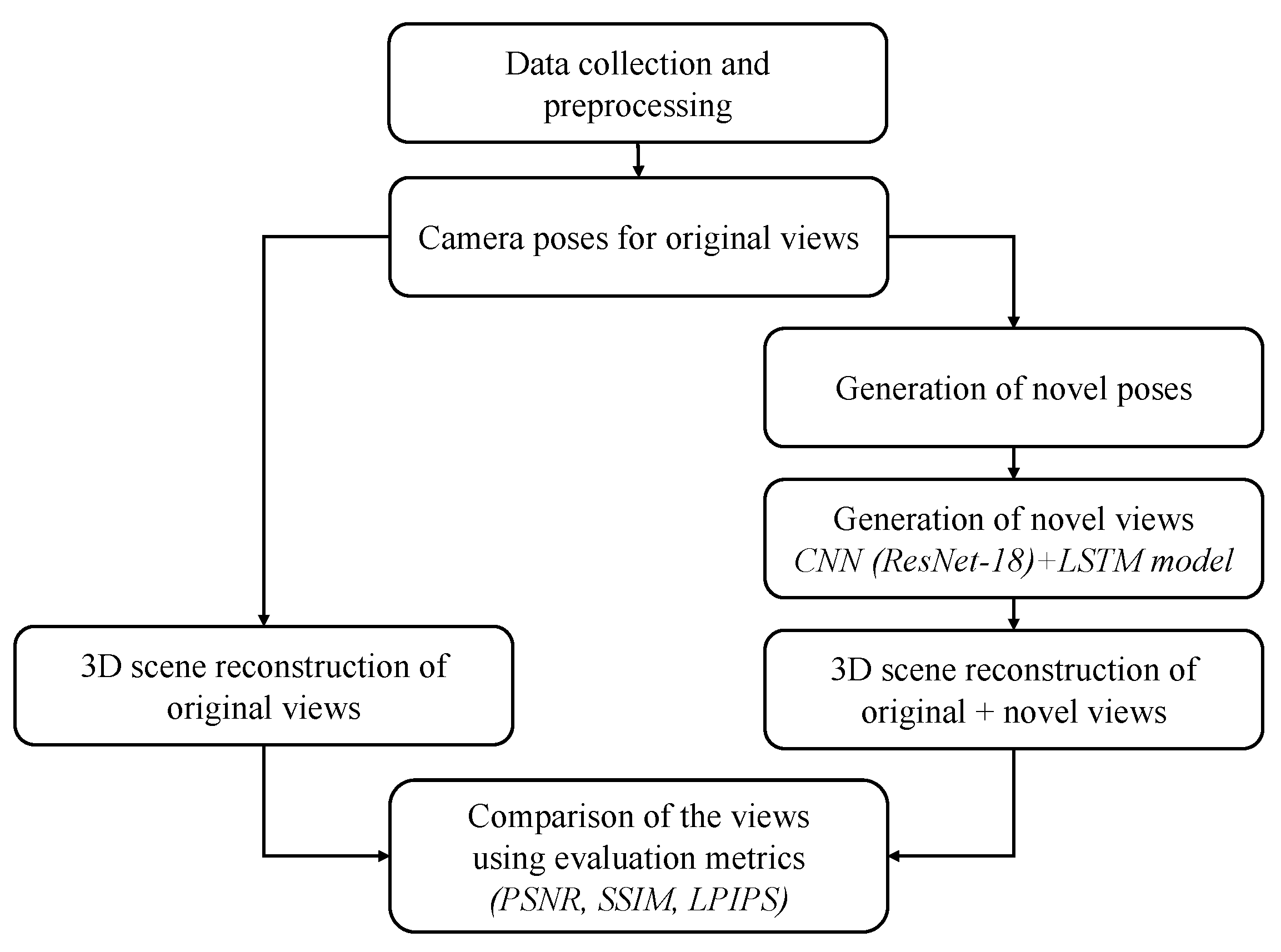Figure 1 illustrates the overall workflow of the proposed pipeline, which follows a sequential process rather than an iterative loop. Since each stage is executed only once, no stopping condition is required. The pipeline begins with data collection and preprocessing and concludes with a comparison between reconstructions obtained from the original 25 images and the augmented 35-image dataset.

The proposed methodology enhances the LLFF framework to tackle sparse light field limitations, improving depth accuracy and occlusion handling in 3D scene reconstruction. To mitigate these issues, synthetic views supplement the initial dataset, establishing a more continuous scene representation. Starting with camera poses computed by COLMAP, interpolation and extrapolation techniques generate new pose viewpoints that expand spatial coverage. We use the 25 + 10 setting to represent a practical sparse-capture scenario and a balanced augmentation level for improving downstream reconstruction with existing technologies such as LLFF, NeRF, and 3D Gaussian Splatting. The 25 input views provide sufficient coverage for stable pose estimation and baseline reconstruction while still exhibiting artifacts due to sparse sampling. We then add 10 synthesized views (40 percent augmentation) to meaningfully reduce viewpoint gaps and improve view continuity without introducing excessive computational overhead or increasing the risk of accumulated synthesis errors from generating too many synthetic images. This augmented dataset allows LLFF to leverage a more densely distributed set of poses, ultimately yielding high-fidelity 3D models that are visually coherent and artifact-free for immersive applications. Beyond LLFF, the same augmented dataset with our generated novel views also improves the performance of Neural Radiance Field (NeRF) and 3D Gaussian Splatting reconstructions, demonstrating that increased dataset density consistently enhances quality across different state-of-the-art rendering approaches.

3.1. Collection of Data and Preprocessing

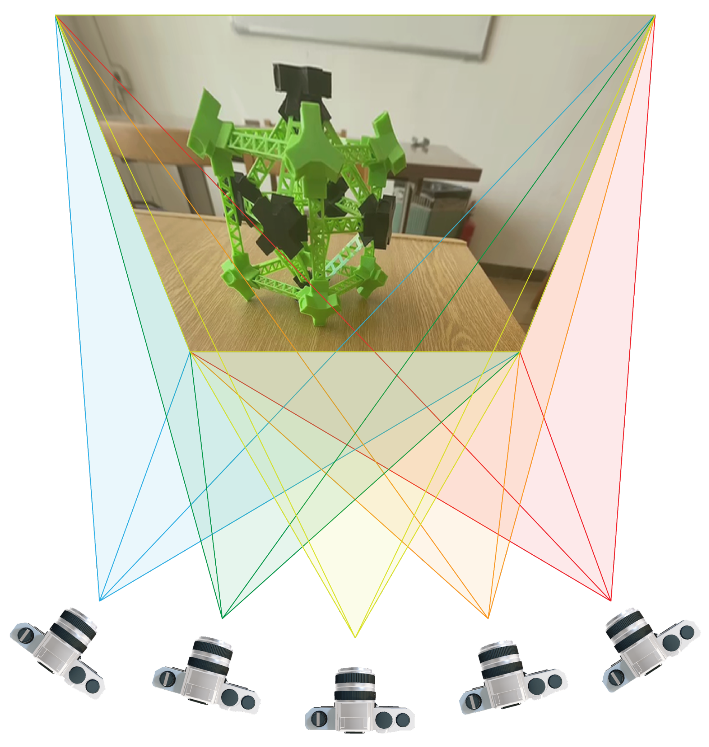
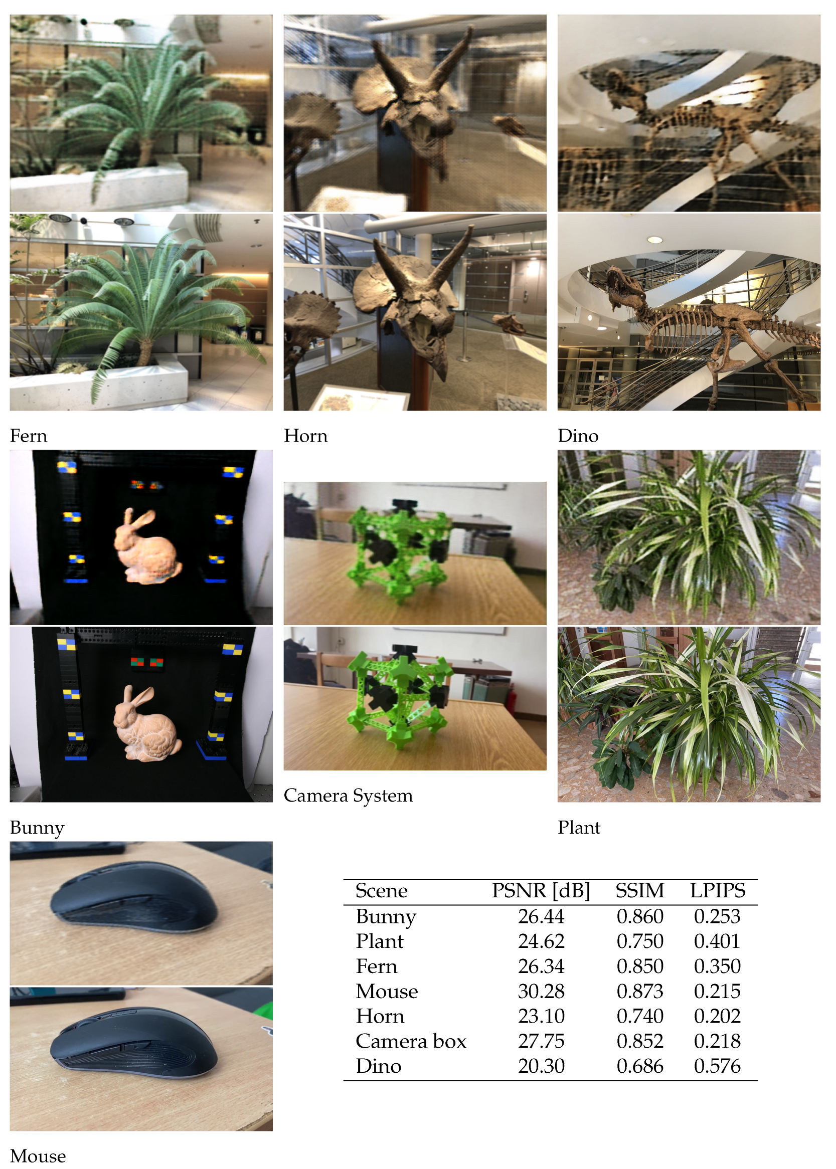
Initially, the authors captured scenes from multiple viewpoints using an iPhone 11, providing a diverse set of perspectives essential for comprehensive scene coverage, as shown in Figure 2. The collected images cover three individual scenes: a computer mouse, a plant, and a camera box. In addition to these, other benchmark scene datasets were used during the experiments: namely, dinosaur, horn, and fern adopted from [19], and the Stanford Bunny [27] was included as the last dataset category.

During data preprocessing, images were standardized to a uniform resolution by downsampling, carefully preserving spatial fidelity and essential visual features for optimizing computational efficiency, memory usage, and processing speed. This technology also helps to improve depth estimation by smoothing noise to ensure that the pipeline remains more efficient without exceeding GPU memory limits. These preprocessing techniques effectively prepare the dataset for high-fidelity synthetic novel view generation and robust 3D scene reconstruction.

3.2. Generation of Novel Camera Poses Through Interpolation Using Translation and Quaternion-Based Rotation and Extrapolation

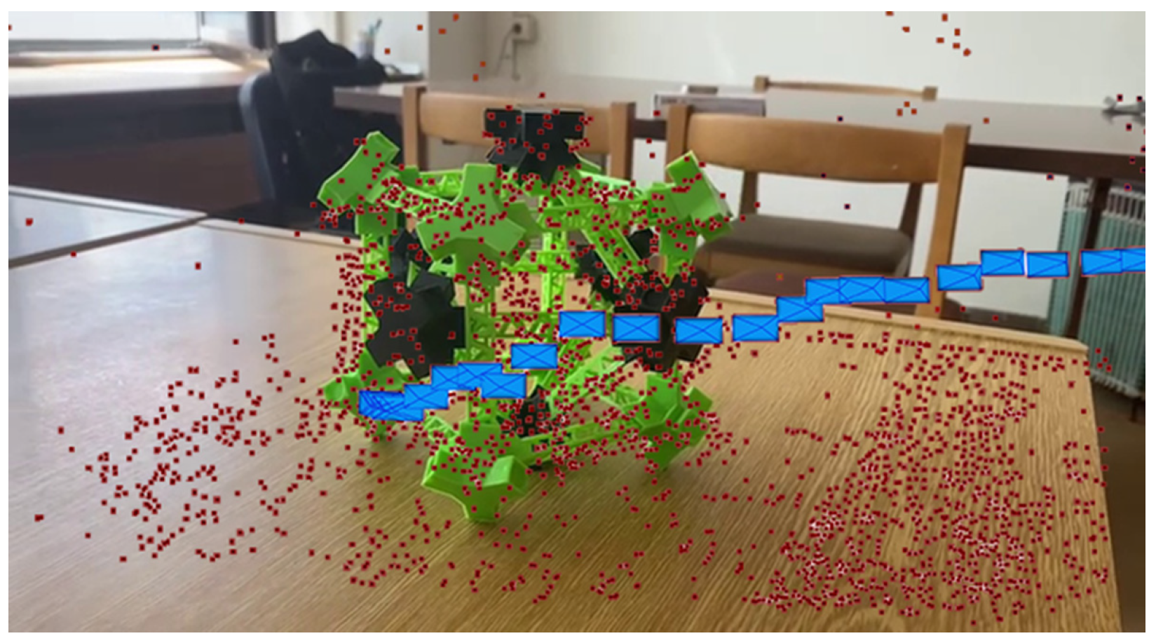
Pose interpolation in sparse light field rendering enables the generation of intermediate views by applying LERP (linear interpolation) to camera translations and SLERP (spherical linear interpolation) to camera rotations represented as unit quaternions, ensuring a smooth rotation path with constant angular velocity. In this work, COLMAP-derived camera poses from a preprocessed dataset serve as the foundation for predicting smooth, high-fidelity transitions between discrete camera positions. COLMAP’s Structure-from-Motion pipeline extracts features, matches keypoints across images, and performs sparse reconstruction to optimize camera poses. This results in a precise 3D spatial configuration, facilitating view synthesis and enhanced 3D scene reconstruction as shown in Figure 3.

To generate 10 novel camera poses based on the 25 original poses from COLMAP corresponding to the original 25 images, interpolation techniques on both the translation position and rotation orientation components of each pose can be used. Each camera pose consists of the aspects detailed in the following subsections.

3.2.1. Translation Vector

For translation interpolation, the LERP (linear interpolation) method is used, as it creates a straight-line path between two translation vectors and provides intermediate positions. Each translation vector can be expressed as $T_i=(x_i,y_i,z_i)$, representing its 3D position. Given two consecutive poses, namely, Pose A with translation vector $T_A=(x_A,y_A,z_A)$ and Pose B with translation vector $T_B=(x_B,y_B,z_B)$, we calculate an interpolated translation $T_{interp}$ at an interpolation parameter t (where $0\le t\le 1$) as follows [28]:

$$T_{interp}=(1-t).T_A+t.T_B$$

(1)

Here,

• $t=0$ corresponds to the original position of Pose A;
• $t=1$ corresponds to Pose B;
• $0<t<1$ yields intermediate positions along the line between $T_A$ and $T_B$.

To create new camera poses, we selected values of t, for example, from 0.1 to 0.9, between each pair of the original 25 poses. These values determine the relative position of each interpolated pose along the line segment between two consecutive poses, enabling smooth intermediate positions. This results in multiple interpolated positions that form the translation component of the novel views, and in the present work, the value of t was 0.5.

3.2.2. Rotation Quaternion

The above-mentioned method is perfectly suitable for translations because the points lie in Euclidean space, and the shortest path between two points is simply a straight line. For two positions $T_A$ and $T_B$ in ${\mathbb{R}}^3$, the interpolated translation at parameter t is given by

$$T_t=(1-t).T_A+t.T_B,0\le t\le 1,$$

(2)

which traces the direct segment between $T_A$ and $T_B$. However, when interpolating rotations, the situation changes entirely. We explain more about rotation interpolation in Appendix A.

In our work, we apply SLERP to generate intermediate orientations between consecutive camera poses. For each pair $(q_1,q_2)$, we compute $\theta$ from the dot product, adjust the sign of $q_2$ if necessary to ensure the shortest arc, and then use the SLERP formula with $t=0.5$ to produce a midpoint orientation:

$$q_{mid}={\displaystyle \frac{sin\frac{\theta }{2}}{sin\theta }}.(q_1+q_2).$$

(3)

Repeating this process for selected pose pairs produces smoothly varying rotations that align with the intended camera trajectory, maintaining constant rotational speed and unit length throughout.

3.2.3. Extrapolating Poses

Extrapolation of the camera poses refers to the generation of novel camera positions and orientations that extend beyond the range of the original camera poses, effectively predicting camera views that lie outside the captured sequence. In this work, extrapolation is used to generate novel camera poses by extending the camera’s trajectory beyond the range of the original sequence. For each pair, an extrapolation factor $t=1.2$ is applied, meaning that the interpolated rotation and position are calculated slightly beyond the second pose in each pair. The choice of $t=1.2$ provides a moderate extension without deviating too far from the existing trajectory, effectively producing a pose that appears just beyond the original endpoint. The translation is calculated by extending the line between the two poses, while the rotation is extrapolated by SLERP, maintaining a smooth continuation of the camera’s path. This approach generates two additional poses that give a sense of progression beyond the last captured views, adding spatial coverage to the scene. A total of 10 novel camera poses are generated by interpolating 8 midpoints between consecutive original poses and extrapolating 2 poses beyond the final positions. Each pose includes translation and quaternion components, ensuring smooth transitions and continuity in camera movement, yielding a comprehensive set of 35 poses as shown in the figure above.

3.3. Generation of Novel Views Corresponding to the Novel Poses (CNN and LSTM)

The CNN–LSTM hybrid model is employed to generate novel views for interpolated and extrapolated camera poses. While Transformer-based fusion and diffusion models excel in unconstrained image generation, they are not well aligned with the demands of pose-conditioned view densification. Self-attention treats views as an unordered set and scales quadratically with the number of input tokens, which weakens the sequential structure inherent in camera trajectory interpolation. Diffusion-based approaches can also introduce stochastic view-to-view variation, which may undermine the geometric consistency required by downstream NeRF and 3DGS pipelines. Our CNN–LSTM backbone addresses these issues by combining a convolutional frontend that extracts multi-scale spatial correspondences from sparse inputs with a recurrent module that maintains a hidden state as a compact geometric memory. This design smooths pose transitions, suppresses hallucinated structure, and enforces cross-view consistency along the generated sequence. It also generalizes across scenes without per-scene optimization and produces deterministic single-pass outputs that integrate directly into existing LLFF, NeRF, and 3DGS workflows, making densification practical and computationally tractable as a preprocessing stage across diverse scene types. 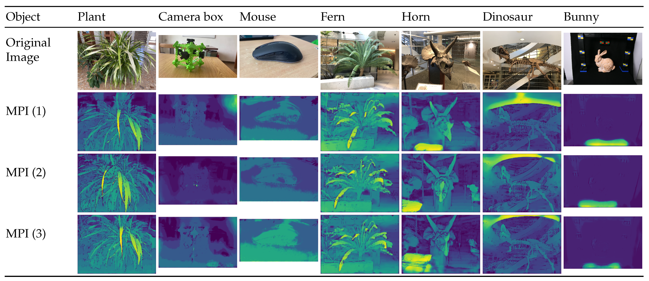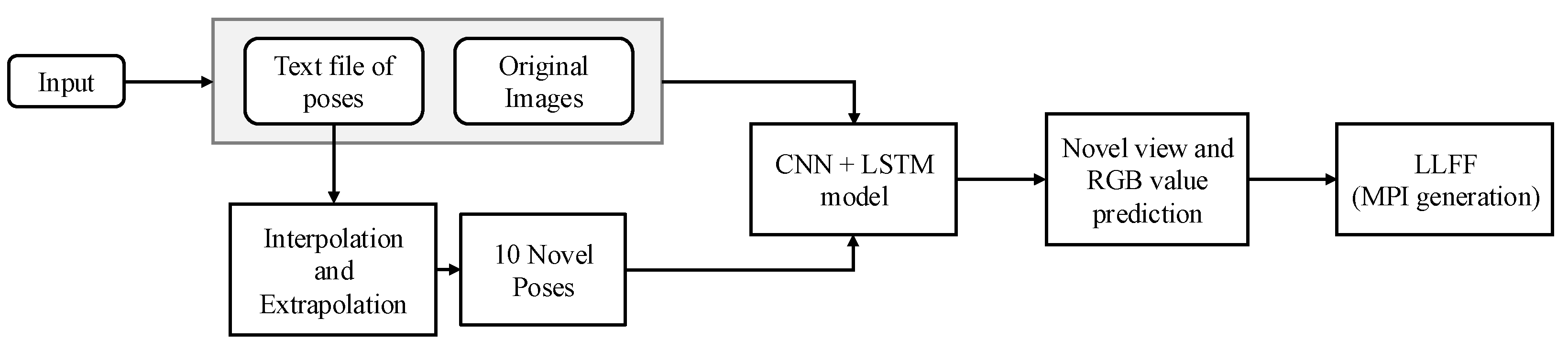Figure 4 illustrates the overall workflow of this process. During training, only the original 25 images and their corresponding 25 camera poses are used to learn the mapping between poses and image content. After training is completed, interpolation and extrapolation techniques are applied to the camera trajectory to produce 10 additional novel poses. These new poses are then provided to the trained CNN–LSTM model, which predicts the corresponding 10 novel views and RGB values. Finally, the original and generated novel images are used for 3D scene reconstruction with LLFF, NeRF, and 3D Gaussian Splatting. Multi-plane image (MPI) generation is the process of decomposing a scene from input views into a stack of RGBA fronto-parallel planes at discrete depth levels, which are then alpha-composited to render novel viewpoints.

This architecture leverages convolutional layers to extract scene features while the LSTM component models temporal continuity across poses, ensuring that generated views remain spatially consistent with the original images. By combining interpolated and extrapolated camera poses with learned pose–image relationships, the model produces novel views that are both geometrically aligned and visually coherent. This enriched dataset improves reconstruction fidelity and reduces artifacts caused by sparse input views.

3.3.1. Feature Extraction via CNN Backbone

The CNN feature extractor in our model is based on the ImageNet-pretrained ResNet-18 backbone, comprising 18 convolutional layers, which is adapted to serve as a high-quality and task-agnostic image encoder for our CNN–LSTM framework.

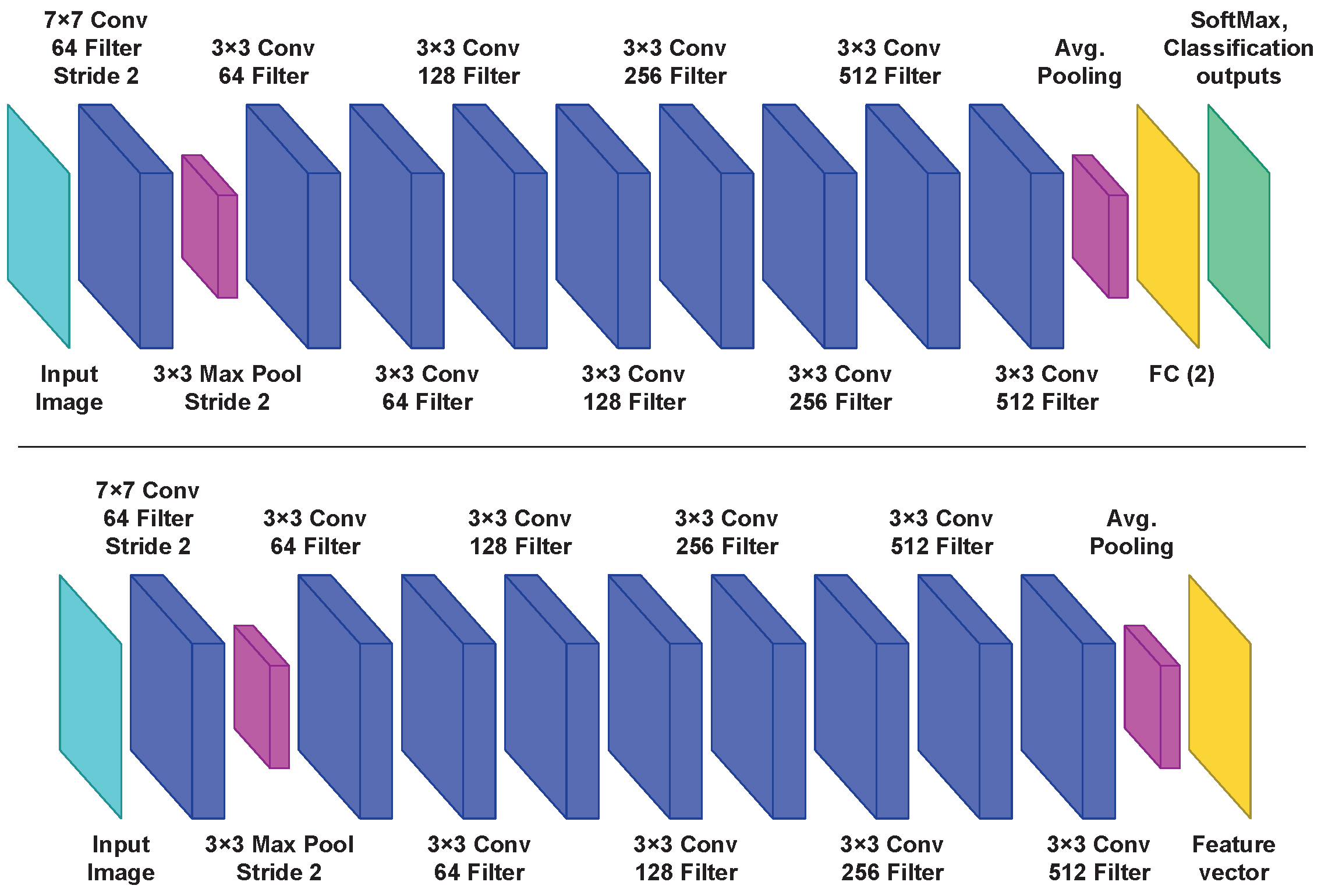
This backbone processes input images through a deep stack of convolutional and residual layers to produce compact but information-rich feature vectors that can be integrated with pose and positional encodings for temporal modeling. Figure 5 provides a direct visual comparison between the standard ResNet-18 architecture and the modified version adopted in our CNN–LSTM framework for feature extraction. In the original ResNet-18 configuration shown in the top row, the input is an RGB image that first passes through a 7 × 7 convolution with 64 learnable filters and a stride of 2, with padding to preserve the receptive field. This is followed by batch normalization, a ReLU activation, and then a 3 × 3 max-pooling layer with a stride of 2. This initial stem reduces the spatial resolution significantly while capturing low-level edge and texture information. The feature maps then pass through successive groups of residual blocks in which the number of channels increases from 64 to 128, 256, and finally 512 while the spatial resolution decreases correspondingly at downsampling stages. Each residual block contains two 3 × 3 convolutions, and each of these is followed by batch normalization and a ReLU activation. The defining skip connection adds the input tensor x to the block’s transformation conv(x), as expressed by

$$F\left(x\right)=x+conv\left(x\right),$$

(4)

where the convolutional operation is defined as

$$conv\left(x\right)=W\ast x+b,$$

(5)

with W representing the learned filters, b the bias term and * denoting convolution. By the end of the final convolutional stage, the representation has 512 channels with a spatial size of 7 × 7 for our input resolution, producing a rich activation tensor of shape 512 × 7 × 7 that encodes high-level semantic and spatial structure from the original image. In the standard classification-oriented ResNet-18, this tensor is passed to a global average pooling layer that collapses each of the 512 feature maps to a single scalar by averaging over its 7 × 7 spatial positions. This yields a compact 512-dimensional vector which is then fed into a fully connected (FC) layer producing 1000 logits or, in some cases, task-specific logits such as 2-way outputs shown in the example figure, and finally a softmax function to obtain class probabilities.

In our modified configuration shown in the bottom row, the convolutional stages and the global average pooling operation are retained exactly as in the original, but the classification fully connected (FC) layer and the subsequent softmax activation are entirely removed. Instead, the pooled 512-dimensional output is treated as the final image descriptor, which serves as a task-agnostic feature vector. This vector is then passed through an additional fully connected layer with 512 outputs in our CNN feature extractor, which serves to project the representation into a space compatible with the concatenation of positional encodings and pose embeddings before being processed by the LSTM. The removal of the classification head is a deliberate modification that discards parameters specialized for ImageNet categories and instead preserves the general-purpose spatial–semantic encoding learned by the convolutional backbone. In our implementation, the ResNet-18 weights are initialized from ImageNet pretraining and are fine-tuned end-to-end along with the rest of the network, which allows the pretrained filters to adapt from generic object recognition features to the specific requirements of view synthesis in our dataset. Since the backbone has already been trained on a vast and diverse dataset, this process benefits from transfer learning and does not require training the convolutional network from the ground up. As a result, the computational burden is significantly reduced, and the CNN part does not demand extensive hardware resources. The use of the global average pooling here is critical because it enables the fixed-length 512-dimensional representation regardless of the input resolution, ensuring that downstream components receive a consistent and information-rich embedding while keeping the parameter count and computational overhead manageable. By directly substituting the classification head with this feature vector pathway, the modified backbone transforms ResNet-18 from a category predictor into a robust visual encoder that integrates efficiently with temporal modeling components.

3.3.2. Pose Embedding and Positional Encoding

To incorporate spatial information from each camera pose, our model uses a fully connected pose embedding layer implemented as a single-layer multilayer perceptron (MLP). Each camera pose is represented as a 7-dimensional vector, with the first three values $(t_x,t_y,t_z)$ representing translation in 3D space and the remaining four values $(q_w,q_x,q_y,q_z)$ representing rotation in quaternion form. The pose embedding layer projects this 7-dimensional vector into a 128-dimensional embedding space through a linear transformation:

$$pose\_embedding=W_p.Pose+b_p,$$

(6)

where

• $Pose$ is the 7-dimensional input vector $[t_x,t_y,t_z,q_w,q_x,q_y,q_z]$,
• $W_p$ is a learnable weight matrix of size 128 × 7 that transforms the input vector into the embedding space, and
• $b_p$ is a learnable 128-dimensional bias vector.

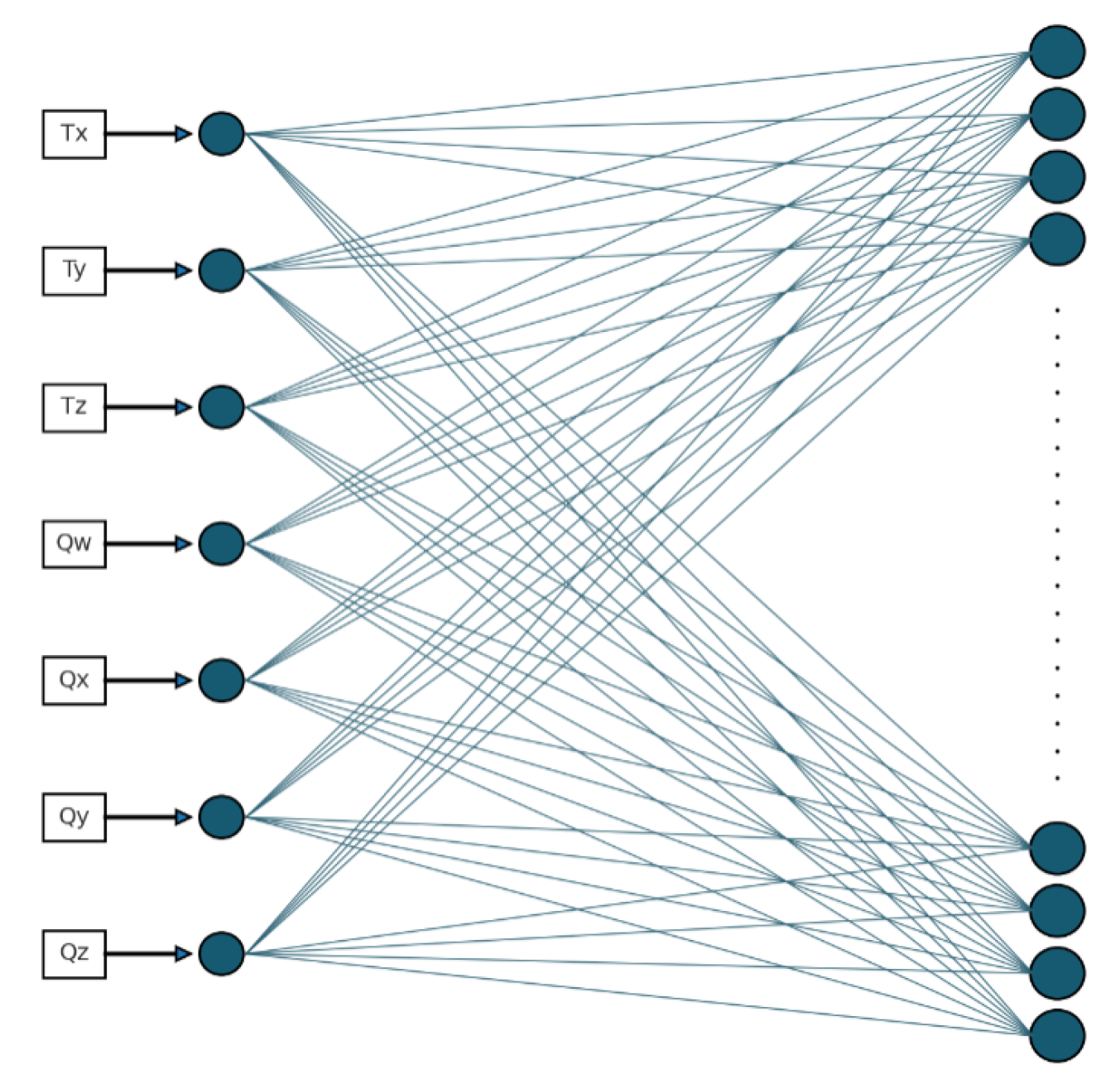
This process can be understood as a fully connected layer with 7 input neurons and 128 output neurons, where each output neuron is connected to every input neuron through a learned weight and bias. The resulting 128-dimensional vector captures the geometric and orientation-specific information of each pose in a compact and high-dimensional form. This allows the model to distinguish between original poses and those obtained via interpolation or extrapolation, enabling smooth continuity in novel view synthesis.

Figure 6 illustrates this MLP structure. On the left, each input node corresponds to one of the seven pose parameters, which are three translations and four quaternion components. These connect through fully dense connections to the output layer shown on the right, which contains 128 neurons, and only a few are depicted for clarity. This dense mapping enables every pose parameter to contribute to every feature in the embedding vector, ensuring that both position and orientation jointly influence the representation.

In addition to the spatial information captured by the pose embedding, the model incorporates a positional encoding mechanism to provide temporal context for each frame in the sequence without introducing additional trainable parameters. Inspired by Transformer architectures [29], this encoding uses fixed sinusoidal functions with both sine and cosine to generate unique representations for each frame index pos within a fixed-length vector. The encoding is defined as follows:

$$\begin{array}{c}Po{s}_{enc}(pos,2i)=sin(pos/{\mathrm{10,000}}^{{\displaystyle \frac{2i}{d}}}),\end{array}$$

(7)

$$\begin{array}{c}Po{s}_{enc}(pos,2i+1)=cos(pos/{\mathrm{10,000}}^{{\displaystyle \frac{2i}{d}}}).\end{array}$$

(8)

Here, d is the dimensionality of the encoding vector, which is set to 512. The variable pos denotes the position index of the frame within the sequence, while i is the dimension index within the encoding vector. The formulation generates smoothly varying values across dimensions using a range of frequencies, enabling the encoding to capture both long-range dependencies and fine-grained temporal relationships. Since the encoding is non-trainable, it preserves continuity and generalizes well to sequences of different lengths. By providing a stable temporal reference frame, the positional encoding complements the spatial pose embedding and enables the LSTM to maintain coherence and produce smooth transitions across both original and novel views in the generated sequence.

3.3.3. LSTM for Sequence Modeling

The LSTM component consists of two stacked LSTM layers, and each contains 512 hidden units. It operates on a rich, multi-source input that captures spatial, temporal, and geometric cues for every frame in the sequence. The network uses the hyperbolic tangent activation function for internal state computations and the sigmoid activation function for its gating mechanisms, including input, output, and forget gates, which control how information is retained or discarded as the sequence progresses.

After the sequence is processed, the output from the final time step is passed through a fully connected layer that reshapes it into an image of the target dimensions. This two-layer LSTM with 512 hidden units plays a key role in modeling temporal dependencies between consecutive camera poses, enabling smooth novel view generation. By maintaining relevant information over time, it learns how viewpoints transition across the sequence to produce high-fidelity images that align with the intended camera trajectory.

Structure and Input Composition

At each time step t, the LSTM receives a 1152-dimensional vector formed by concatenating three distinct components. The first component is a 512-dimensional CNN feature vector that encodes the scene’s high-level spatial content. The second component is a 512-dimensional sinusoidal positional encoding that provides temporal context by indicating the frame’s order within the sequence. The third component is a 128-dimensional pose embedding that represents the camera’s position and orientation through translation and quaternion rotation, as shown in Figure 7. This unified representation ensures that the LSTM processes not just visual appearance, but also the geometric context and temporal ordering necessary for novel view synthesis.

Gate Operations and Information Flow

The LSTM processes each input at time step t using three primary gates, which are the input gate, forget gate, and output gate. These gates effectively regulate information flow, enabling selective retention of essential details while discarding less relevant information. The input gate ($i_t$) controls the addition of new input information to the cell state ($c_t$), contributing to the LSTM’s long-term memory. The forget gate ($f_t$) determines the portion of the previous cell state ($c_{t-1}$) that should be retained, thereby allowing the model to “forget” details that are no longer pertinent as the sequence advances. The output gate ($o_t$) governs the creation of the hidden state ($h_t$), which serves as the model’s short-term memory and facilitates the generation of the next output. These gates collaboratively update the cell state as follows [30]:

$$c_t=f_t\odot c_t-1+i_t\odot tanh(W_c.x_t+U_c.t_t-1+b_c),$$

(9)

where ⊙ denotes element-wise multiplication. This gating structure enables the LSTM to learn long-term dependencies across frames, ensuring the model can produce smooth and temporally coherent images that accurately reflect the camera’s movement trajectory.

3.3.4. Output Layer for Image Prediction

Once the sequence modeling is complete, the final hidden state of the LSTM at each time step is passed through a fully connected output layer. This layer transforms the hidden state into an RGB image aligned with the corresponding novel camera pose:

$$Output=W_{out}.h_t+b_{out},$$

(10)

where $W_{out}$ and $b_{out}$ are learned weights and biases. Acting as a decoder, this output layer maps the high-level feature vector into pixel values for an image with three channels, and the height and width of the input images. The layer produces a flattened image representation that is reshaped into the final image dimensions, generating an RGB image that visually corresponds to each novel pose.

3.3.5. Training Process and Optimization

Training is performed using a carefully selected set of configurations to ensure stable convergence and high-quality image synthesis. We adopt the Adam optimizer, chosen for its adaptive learning rate, which enables efficient and precise weight updates during training. This choice allows the model to adjust learning dynamics automatically, making it robust to different stages of optimization while avoiding the pitfalls of static learning rate schedules. The Adam update rule is represented by the following:

$${\theta }_{t+1}={\theta }_t-\alpha .{\displaystyle \frac{m_t}{ϵ+\sqrt{v_t}}},$$

(11)

where $\alpha$ is the learning rate, which is set to 0.001 to strike a balance between convergence speed and stability, $m_t$ and $v_t$ represent the bias-corrected first and second moment estimates, while $ϵ$ is a small constant that prevents division by zero. Given the dataset size and memory considerations, the batch size is set to 1 due to sequential input layout and high spatial resolution, and the model is trained for 100 epochs. The model employs mean squared error (MSE) loss to minimize the difference between predicted and ground-truth images, which is calculated as [31]:

$$MSE={\displaystyle \frac{1}{N}}\sum _{i=1}^N{(y_i-{\widehat{y}}_i)}^2,$$

(12)

where $y_i$ represents the true pixel values and ${\widehat{y}}_i$ represents the predicted values. The loss function enforces visual accuracy by reducing pixel-level discrepancies between generated and original frames, thereby enhancing generalization to novel camera poses. Training further benefits from Automatic Mixed Precision (AMP) with gradient scaling, which optimizes memory usage and speeds up computation, making the approach well-suited for deep CNN–LSTM architectures.

In our framework, the CNN component is based on the ResNet-18 model, which encodes each input frame into a 512-dimensional feature vector capturing essential spatial information. We fine-tune this model rather than training from scratch, reducing the number of learnable parameters while retaining adaptability to our dataset. These features, along with positional encodings and pose embeddings, are processed by a two-layer LSTM with 512 hidden units, which effectively models temporal dependencies required for high-fidelity view synthesis under novel poses.

Training is performed on a Windows 11 workstation equipped with an AMD Ryzen Threadripper PRO 3955WX processor with 16 cores, 128 GB of RAM, and a single NVIDIA GeForce RTX 4090 GPU with 24 GB of VRAM. The software stack consists of Python 3.10, PyTorch 2.5.1 with a CUDA 12.1 backend and cuDNN acceleration. Each training sequence contains 25 images. On this setup, complete training of one 25-image scene requires approximately 15.7 min, with the training loss converging to $1.5\times {10}^{-5}$. Inference on the same hardware takes 0.147 s on average per image, and generating 10 novel views requires 1.38 s in total.

Our training time per scene is a bit longer than the quickest results reported for 3D Gaussian Splatting when it is trained with a small number of iterations. However, such timing depends heavily on how many iterations are used and what quality is targeted, so a direct comparison is not always fair. The important point is that our inference speed is close to modern real-time rendering methods. This means our system can be used in interactive or time-sensitive applications, producing novel views almost instantly while keeping high visual quality.

3.4. Unique Aspects of the Model Design

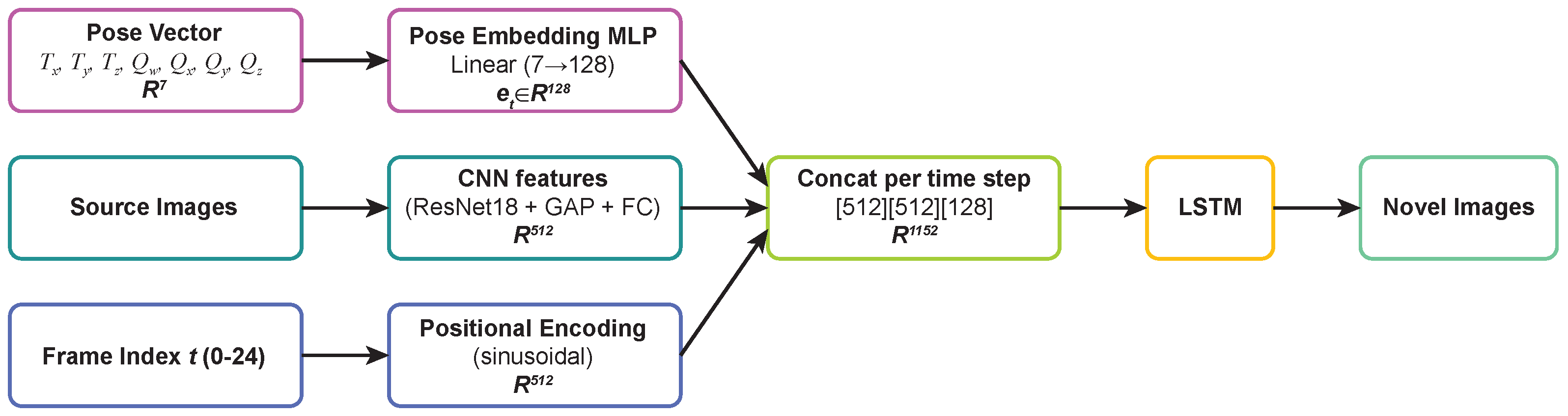
The proposed CNN-LSTM architecture combines CNN-based spatial feature extraction, LSTM-based temporal modeling, and positional encoding to generate high-fidelity images aligned with novel camera poses, achieving spatial and temporal coherence. By embedding pose and positional context, the model distinguishes between original and interpolated and extrapolated views, creating smooth transitions across frames. This method enables effective 3D scene reconstruction from sparse light fields, synthesizing realistic intermediate views. As a result, it enhances spatial and depth fidelity, even with limited initial poses, delivering continuous and geometrically consistent scene representations, as shown in Figure 8.

The CNN extracts detailed spatial features from each sparse view while the LSTM captures temporal dependencies between poses, maintaining continuity in the camera’s movement through the scene. Positional embeddings provide additional context, helping the model understand each pose’s position within the sequence, allowing it to generate geometrically consistent intermediate views. This approach effectively reconstructs 3D scenes by interpolating within the sparse light field, yielding realistic and continuous transitions that enhance the spatial and depth fidelity of the reconstructed environment.

3.5. Multi-Plane Image (MPI) Representation and LLFF Pipeline

The multi-plane image (MPI) representation in the LLFF [11] pipeline organizes the scene into depth-aligned planes, each containing RGB and alpha values to capture color and transparency across depths. Ray bundles from each camera view are globally aligned, with homography transformations projecting images onto depth planes to maintain spatial consistency. Alpha blending refines visibility by layering nearer objects over farther ones, achieving smooth transitions and depth coherence in rendered views. Mathematically, the projection onto depth planes uses homography transformations for each depth level, where each plane k has depth dk and homography $H_k=K(\mathrm{d}k,P)$ calculated from the camera parameters. To blend RGB and alpha values across depth planes, the final color C(p) at each pixel p is given by [11]:

$$C\left(p\right)=\sum _{k=1}^k{\alpha }_k\left(p\right).C_k\left(p\right).\prod _{j=1}^{k-1}[1-{\alpha }_j\left(p\right)],$$

(13)

where $C_k\left(p\right)$ is the color in the k-th depth plane and ${\alpha }_k\left(p\right)$ represents opacity. This layered blending allows depth continuity and occlusion handling, which are essential for realistic rendering.

We use a multi-plane image (MPI) with D planes (we denote this plane count as k, that is $k\equiv D$), where each plane stores RGB color and an opacity $\alpha$ (so each plane is RGB$\alpha$), the D planes are placed at depths sampled uniformly in disparity (inverse depth) within the reference-view frustum. For each MPI, we build plane-sweep volumes by reprojecting a 5-view local neighborhood (the reference image plus its 4 nearest cameras in 3D translation space) onto the D disparity planes, predict per-plane RGB$\alpha$, then render a novel target view by homography-warping every plane into the target camera and compositing them back-to-front with the standard Porter–Duff “over” operator (accumulating color C and opacity $\alpha$). When multiple MPIs contribute to the same target pose t, rendering MPI

$$k\to \left(C_{t,k},{\alpha }_{t,k}\right),$$

(14)

and we fuse them with alpha-aware blending

$$C_t={\displaystyle \frac{{\sum }_k{w}_{t,k}{\alpha }_{t,k}{C}_{t,k}}{{\sum }_k{w}_{t,k}{\alpha }_{t,k}}}$$

(15)

where $w_{t,k}$ are view-selection weights: bilinear weights over the 4 nearest MPIs for regularly sampled camera grids, or $w_{t,k}\propto exp(-\gamma \ell (p_t,p_k))$ for irregular sampling, with $\ell (p_t,p_k)={\Vert t_t-t_k\Vert }_2$ being the Euclidean distance between camera translations, $\gamma ={\displaystyle \frac{f}{D{z}_{min}}}$ a scaling constant, f the camera focal length (in pixels), and $z_{min}$ the minimum scene depth used to define the disparity range.

4. Experiments and Subjective Evaluation

Integrating LLFF with a CNN-LSTM model enhances the quality of novel view synthesis by the combination of multi-plane image (MPI) representations, sequential modeling, and spatial feature extraction. LLFF constructs depth-aware MPIs from multiple viewpoints, ensuring accurate scene geometry, while a CNN extracts hierarchical spatial features from the input images. The LSTM models viewpoint transformations across sequential images, learning temporal dependencies to improve depth consistency and smooth view interpolation. This section presents the experiments performed on the selected scenes and the corresponding results and evaluation.

4.1. Constructing and Compositing Multi-Plane Images (MPIs)

Multi-plane images (MPIs) are a representation technique used in light field rendering and 3D scene reconstruction. An MPI divides the scene into multiple depth-aligned planes, each representing a different layer of the light field at various depths. Each plane contains both RGB color information and alpha values for opacity, allowing for the representation of both color and transparency at different depths. MPIs combine depth-aligned planes for each viewpoint, creating a layered 3D structure that models occlusions and preserves depth fidelity. Smooth transitions are achieved by blending RGB and alpha values across layers, ensuring realistic depth effects and consistent occlusions. The final color composition for each view is achieved by alpha blending across all depth layers, ensuring realistic depth transitions. For a given pixel p, color C(p) is calculated by summing across the layers using a multi-layer alpha composition model as described earlier. A subset of Multi-Plane Images (MPIs) corresponding to the respective objects is illustrated in Figure 9.

4.2. 3D Scene Reconstruction with LLFF (Local Light Field Fusion)

The LLFF [19] framework composites the MPIs into a cohesive 3D representation, enabling spatial navigation across multiple viewpoints. The composite model ensures depth consistency and correct occlusion effects by rendering layers according to their alpha values (transparency or blending weights). This layered rendering preserves depth accuracy, creating a realistic 3D effect and enhancing depth perception for synthesized viewpoints.

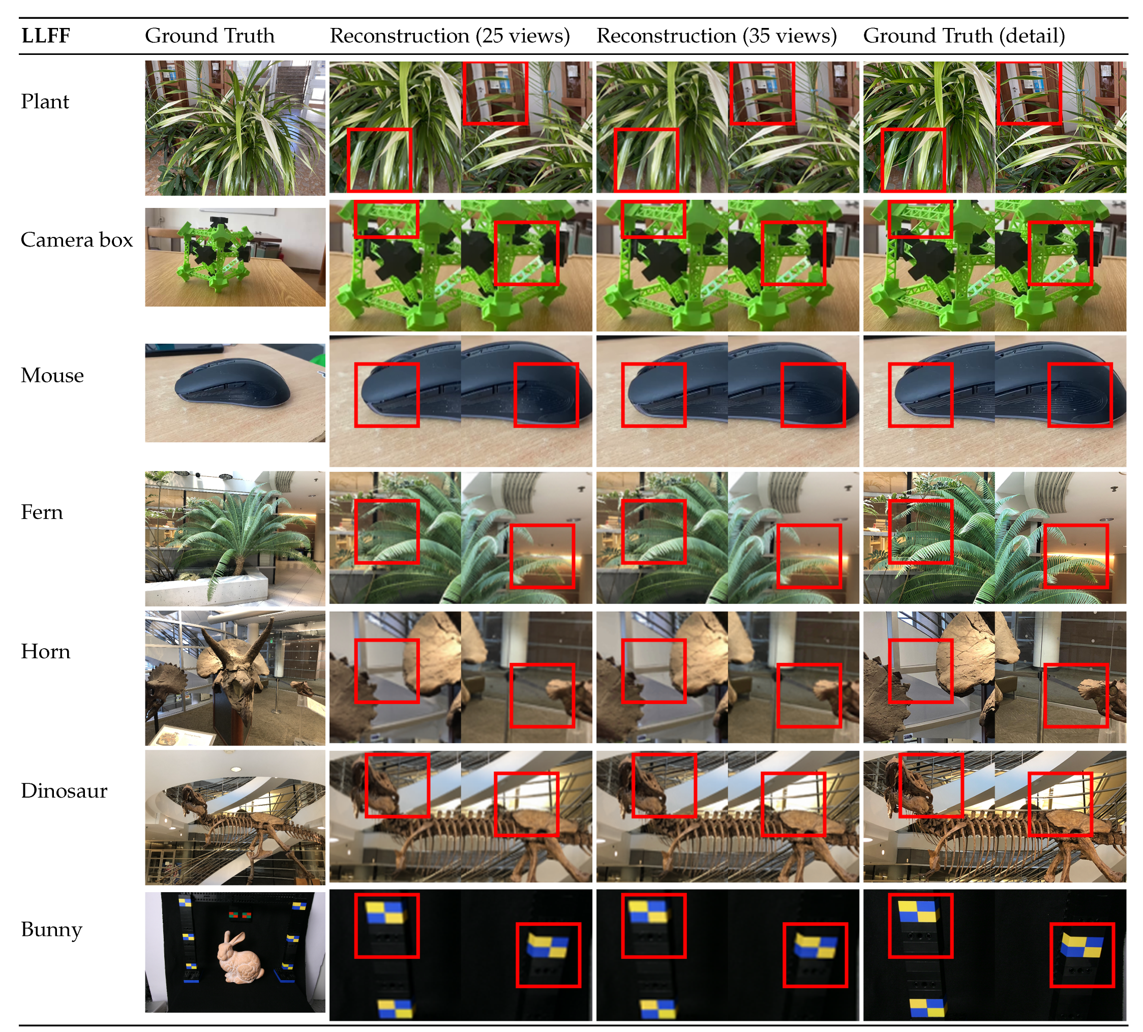
Seven scenes are presented in Figure 10 with corresponding regions marked to compare reconstruction quality across the three setups. The analysis emphasizes that areas with fine and complex details, such as truss joints in the camera box (green 3D-printed structure), are poorly reconstructed with only 25 views. This limitation arises from insufficient visual information, making it challenging to accurately model intricate geometries. In contrast, the 35-view reconstruction significantly improves the representation of such details, closely aligning with the ground truth.

On the other hand, for areas that lack fine details or complexity, such as larger, smoother surfaces or less intricate regions, the 25-view reconstruction performs adequately. These simpler regions require fewer views to capture essential details effectively. However, as demonstrated in the comparison, the addition of more views enhances overall reconstruction quality, even in less demanding areas, resulting in a more robust and faithful representation of the scene.

This comparison underscores the importance of incorporating additional views for reconstructing scenes with fine and intricate details. While fewer views can suffice for simpler geometries, complex regions with great detail density necessitate additional views to ensure fidelity and accuracy. Thus, balancing the number of views based on the complexity of the scene is critical for achieving optimal 3D reconstruction results, as highlighted by the cantilever joint example. For practical applications, especially in scenarios requiring precision, increasing the number of views is a reliable strategy to improve reconstruction quality.

The incorporation of novel views generated by CNN-LSTM into the LLFF framework significantly enhances the quality of both synthesized views and 3D scene reconstructions by increasing the density of input poses and improving the MPI (Multi-Plane Image) representations. Local light field fusion, while capable of generating novel views such as the 26th frame using originally captured 25 input images, often encounters limitations with sparse input data, resulting in interpolation errors in regions with complex structures or occlusions. For addressing this problem, 10 additional novel views generated by CNN-LSTM were introduced, densifying the input pose space and enabling smoother, more accurate interpolations. Unlike LLFF’s linear interpolation methods, the CNN-LSTM model captures non-linear relationships between poses, producing views that align more effectively with the scene’s temporal structure and geometry. These additional views refine the RGB and depth information in MPI layers, leading to sharper textures, improved occlusion handling, and reduced artifacts such as depth discontinuities and color inconsistencies. Missing details in occluded regions are effectively filled using the contextual insights provided by the neural network model.

This enriched MPI representation results in novel views with better clarity, realism, and smooth transitions, making them ideal for applications requiring realistic scene navigation. Furthermore, the reduced angular gaps and improved depth sampling contribute to a more geometrically accurate and visually coherent 3D reconstruction.

4.3. 3D Scene Reconstruction with NeRF

Neural radiance fields (NeRFs) [6] represent scenes as continuous volumetric functions that map 3D coordinates and viewing directions to color and density values, allowing photorealistic novel view synthesis. In our evaluation, NeRF reconstructions were performed using both the original 25 input images and the enhanced 35-image dataset that includes original views and 10 additional novel views generated from interpolated and extrapolated camera poses. The results were evaluated across seven 3D scenes.

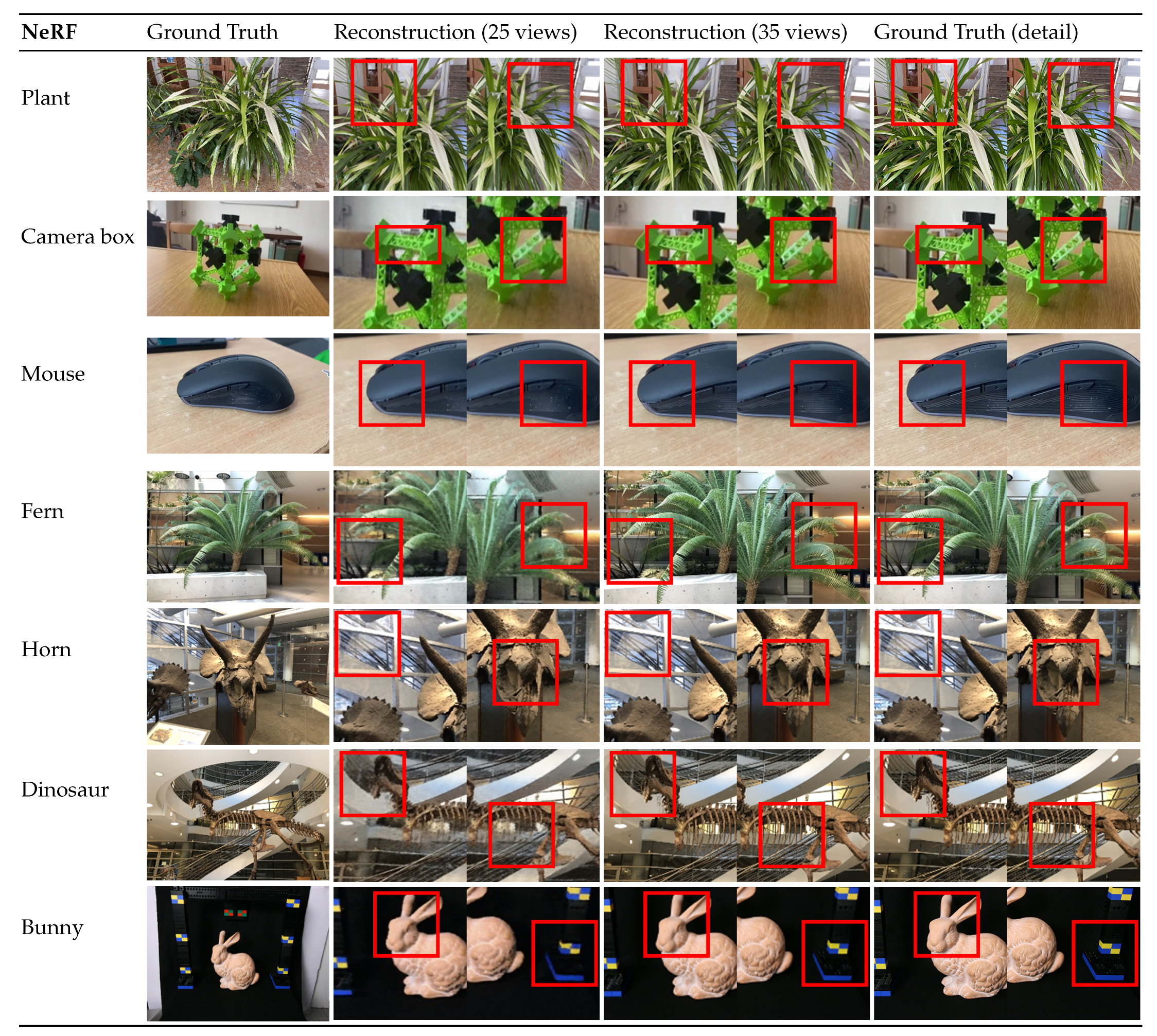
Visual analysis shows that reconstructions with only 25 input views struggle in regions with complex geometry and occlusions, often producing blurry textures or missing structural details. The addition of 10 generated views reduces these limitations, enabling sharper reconstructions that more closely align with the ground truth. As highlighted in Figure 11, fine details such as edges, object contours, and occluded regions are better represented with 35 views.

4.4. 3D Scene Reconstruction with 3D Gaussian Splatting

Three-dimensional (3D) Gaussian Splatting [8] (3DGS) represents scenes as a set of anisotropic 3D Gaussians that jointly encode geometry and appearance, allowing fast and photorealistic rendering from arbitrary viewpoints. In our evaluation, reconstructions were performed using both the original 25 input images and the enhanced 35-image dataset that includes original views and 10 additional novel views generated from interpolated and extrapolated camera poses.

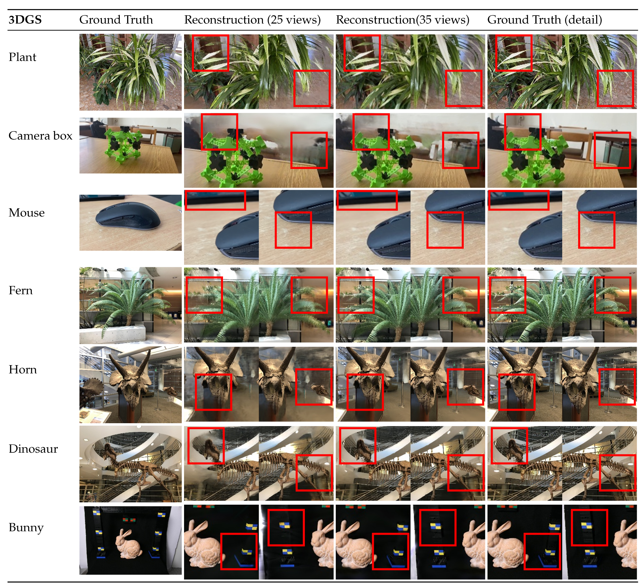
With only 25 input views, 3D Gaussian Splatting reconstructions exhibit visible gaps and incomplete geometry, particularly in regions with high complexity or occlusions. Adding the 10 generated views significantly reduces these artifacts, enabling smoother surface representations and more accurate preservation of fine details. As highlighted in Figure 12, object boundaries, textures, and occluded structures are reconstructed with greater fidelity when 35 views are used.

These results demonstrate that 3D Gaussian Splatting, like other reconstruction methods, benefits strongly from denser view coverage enhanced by our method. The inclusion of generated novel views improves the optimization of the Gaussian primitives, leading to reconstructions that are more complete, visually coherent, and consistent with the ground truth.

4.5. 3D Scene Reconstruction with DietNeRF

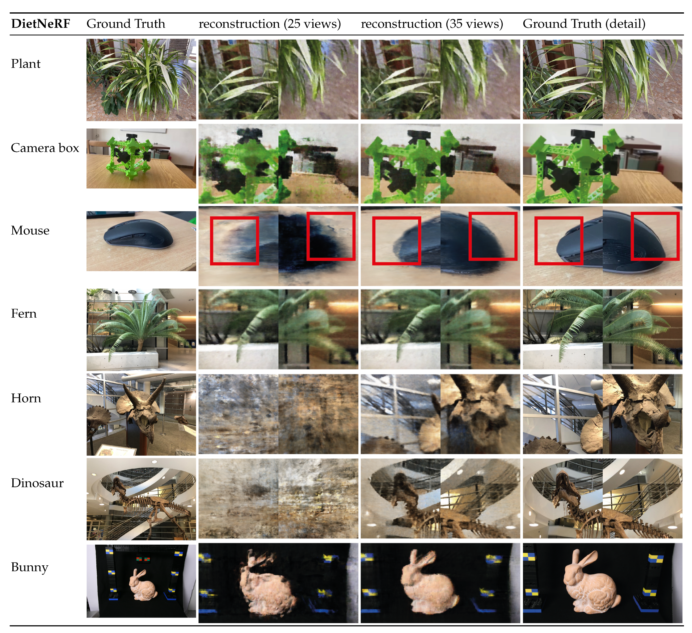
DietNeRF [32] extends the NeRF framework by introducing a semantic feature-space consistency loss that regularizes rendered views under sparse supervision. We evaluate the method using 25 posed RGB images and an augmented 35-view dataset including 10 synthesized views generated via interpolated and extrapolated camera poses. In the 25-view regime, the model exhibits under-constrained optimization, resulting in depth ambiguity, over-smoothed density fields, and attenuation of high-frequency appearance components. Although semantic regularization promotes global structural alignment, it is insufficient to fully resolve local geometric inaccuracies and view-dependent radiance inconsistencies, particularly in occluded or sparsely observed regions.

The inclusion of 10 additional views increases angular sampling density and improves coverage of the scene manifold, thereby reducing pose-induced ambiguities in volumetric rendering. This leads to more stable convergence of the radiance field parameters, with better-conditioned estimation of both volumetric density ($\sigma$) and view-dependent color (c). Consequently, reconstructions exhibit reduced floaters, improved surface continuity, and enhanced recovery of fine-scale details and occluded structures. As shown in Figure 13, the 35-view configuration yields higher geometric completeness and improved photometric consistency, confirming that DietNeRF remains strongly dependent on sufficient multi-view constraints, and that synthesized viewpoints effectively enhance reconstruction fidelity. To evaluate the effectiveness of our approach under sparse-view conditions, we apply DietNeRF using both the original 25 input views and an augmented set that includes additional views generated by our method. While increasing the number of training views is generally expected to improve reconstruction quality, our goal is not merely to increase data quantity, but to synthesize geometrically consistent and informative novel viewpoints derived from limited observations. These generated views effectively expand the scene’s angular coverage and introduce additional multi-view constraints, particularly in regions affected by occlusions or sparse sampling. Consequently, DietNeRF trained on the augmented dataset yields reconstructions with improved structural completeness, sharper details, and enhanced photometric consistency compared to the baseline sparse-view setting.

4.6. Calculation of Horizontal and Vertical Field of View

Field of view (FoV) refers to the extent of the observable world that is seen at any given moment through a camera, optical device, or the human eye. It is typically measured as an angle in degrees and represents how wide or narrow the view is, and the calculation is given as follows:

4.6.1. Horizontal Field of View

$$Fo{V}_{horizontal}=2\times arctan\left({\displaystyle \frac{image\_width}{2\times f}}\right).$$

(16)

Given that the image width is $image\_width=1280pixels$, and $f=1536pixels$, the horizontal field of view $Fo{V}_{horizontal}=2\times arctan\left({\displaystyle \frac{1280}{2\times 1536}}\right)\approx 2\times arctan\left(0.4167\right)\approx {45.24}^{°}$.

4.6.2. Vertical Field of View

$$Fo{V}_{vertical}=2\times arctan\left({\displaystyle \frac{image\_height}{2\times f}}\right).$$

(17)

Given that the image height is $image\_height=960pixels$, the vertical field of view $Fo{V}_{vertical}=2\times arctan\left({\displaystyle \frac{960}{2\times 1536}}\right)\approx 2\times arctan\left(0.3125\right)\approx {34.71}^{°}$.

5. Objective Evaluation

To evaluate the benefit of the generated novel images based on the interpolated and extrapolated poses, we performed qualitative experiments across three reconstruction methods, namely, LLFF, NeRF, and 3D Gaussian Splatting (3DGS). For each method, the pipeline was executed twice, once with the original 25 input images (regarded as original views) and again with the enhanced 35-image dataset that included 10 additional novel views generated from interpolated and extrapolated camera poses along with the 25 original images. The objective was to assess how denser input coverage influenced reconstruction quality. In addition to our captured dataset, most of the datasets used in the evaluation were widely used benchmark datasets in LLFF, NeRF, and 3DGS research, ensuring that the comparison was consistent with standard practice.

5.1. Evaluation Metrics

To quantitatively assess reconstruction quality, we used three widely adopted image quality metrics, namely, structural similarity index metric (SSIM), peak signal-to-noise ratio (PSNR), and learned perceptual image patch similarity (LPIPS) [33]. SSIM, PSNR, and LPIPS were computed only against real captured frames that were held out from training, using their true recorded camera poses as ground truth. For each evaluated pose, the predicted image was compared with the corresponding captured image at the same pose (or within a specified pose-matching tolerance, reported in the paper). Views synthesized at intermediate or extrapolated poses were not treated as ground truth and were excluded from quantitative evaluation unless an actual captured image existed at that pose. The manuscript reports the exact train/test split, the held-out frame/pose indices, and the correspondence between the queried poses and held-out real poses to prevent any evaluation leakage.

These metrics were applied to compare the quality of reconstructions as well as novel view synthesis using 25 original views and 35 views, with ground truth images serving as the reference. SSIM assesses luminance, contrast, and structure to reflect how closely each generated image matches its ground truth counterpart, providing a score between −1 and 1, with 1 indicating identical images.

Table 1. SSIM results for 25 and 35 views compared to ground truth. Best results are in bold.

SSIM ↑	LLFF		NeRF		3DGS		DietNeRF
	25	35	25	35	25	35	25	35
Camera box	0.541	0.743	0.3196	0.5231	0.5068	0.5231	0.346	0.566
Plant	0.282	0.732	0.2610	0.3063	0.4744	0.5529	0.559	0.582
Mouse	0.476	0.736	0.7407	0.9938	0.8456	0.9712	0.448	0.632
Bunny	0.7448	0.7803	0.8047	0.8121	0.7383	0.8505	0.712	0.802
Horn	0.4756	0.5117	0.4245	0.5291	0.6245	0.7007	0.241	0.571
Dinosaur	0.6718	0.7462	0.4550	0.4930	0.6996	0.7321	0.244	0.672
Fern	0.5538	0.5730	0.4633	0.9026	0.7013	0.7561	0.612	0.640
Average	0.534	0.688	0.4951	0.6514	0.6557	0.7266	0.451	0.637

presents the SSIM values obtained in this evaluation.

The peak signal to noise ratio (PSNR) is a metric that measures image quality by comparing the original image to its reconstructed version, focusing on the ratio of signal to noise in decibels (dB). Calculated using the mean squared error (MSE) between images, PSNR incorporates maximum pixel intensity to normalize this error, with higher values indicating closer similarity to the original. For both 25 and 35 image datasets, PSNR values were computed against ground truth images to assess reconstruction quality as shown in

Table 2. PSNR results for 25 and 35 views compared to ground truth.

PSNR ↑	LLFF		NeRF		3DGS		DietNeRF
	25	35	25	35	25	35	25	35
Camera box	30.9	32.4	11.3832	19.1391	18.5837	20.1291	14.370	20.000
Plant	20.97	30.09	15.9525	17.7925	17.433	18.8711	22.013	23.382
Mouse	29.03	33.11	26.1406	45.5864	36.2569	40.2660	18.898	24.911
Bunny	17.24	20.09	20.1194	20.5242	13.1016	21.4247	19.594	24.631
Horn	11.869	14.274	15.2894	18.8414	18.7915	21.3606	12.755	22.923
Dinosaur	18.263	22.467	15.3124	18.5207	18.9847	20.0958	12.184	23.124
Fern	16.041	17.774	12.1658	32.3443	20.3699	22.000	22.471	23.323
Average	20.616	24.315	16.623	24.678	20.503	23.449	17.469	23.184

.

The learned perceptual image patch similarity (LPIPS) metric assesses perceptual similarity between images by measuring distances in a deep feature space, leveraging feature embeddings from deep convolutional networks. By normalizing and scaling these activations, LPIPS captures high-level structural similarities, focusing on perceptual closeness rather than pixel-level accuracy. LPIPS was calculated for both sets of 25 and 35 images and compared against the ground truth to evaluate similarity as shown in

Table 3. LPIPS results for 25 and 35 views compared to ground truth.

LPIPS ↓	LLFF		NeRF		3DGS		DietNeRF
	25	35	25	35	25	35	25	35
Camera box	0.168	0.101	0.7556	0.1096	0.1196	0.1096	0.458	0.196
Plant	0.148	0.135	0.3361	0.2962	0.4706	0.3756	0.399	0.363
Mouse	0.388	0.045	0.0705	0.0053	0.0825	0.0694	0.555	0.339
Bunny	0.2303	0.1684	0.2209	0.1794	0.3441	0.2935	0.354	0.268
Horn	0.8955	0.8329	0.3637	0.2292	0.5167	0.4074	0.776	0.584
Dinosaur	0.5265	0.4818	0.3321	0.3043	0.4142	0.3655	0.759	0.429
Fern	0.7177	0.6698	0.8934	0.1564	0.3999	0.3393	0.516	0.510
Average	0.4391	0.3477	0.4246	0.1829	0.3353	0.2800	0.545	0.384

below.

5.2. Comparison of the Values Calculated by Evaluation Metrics

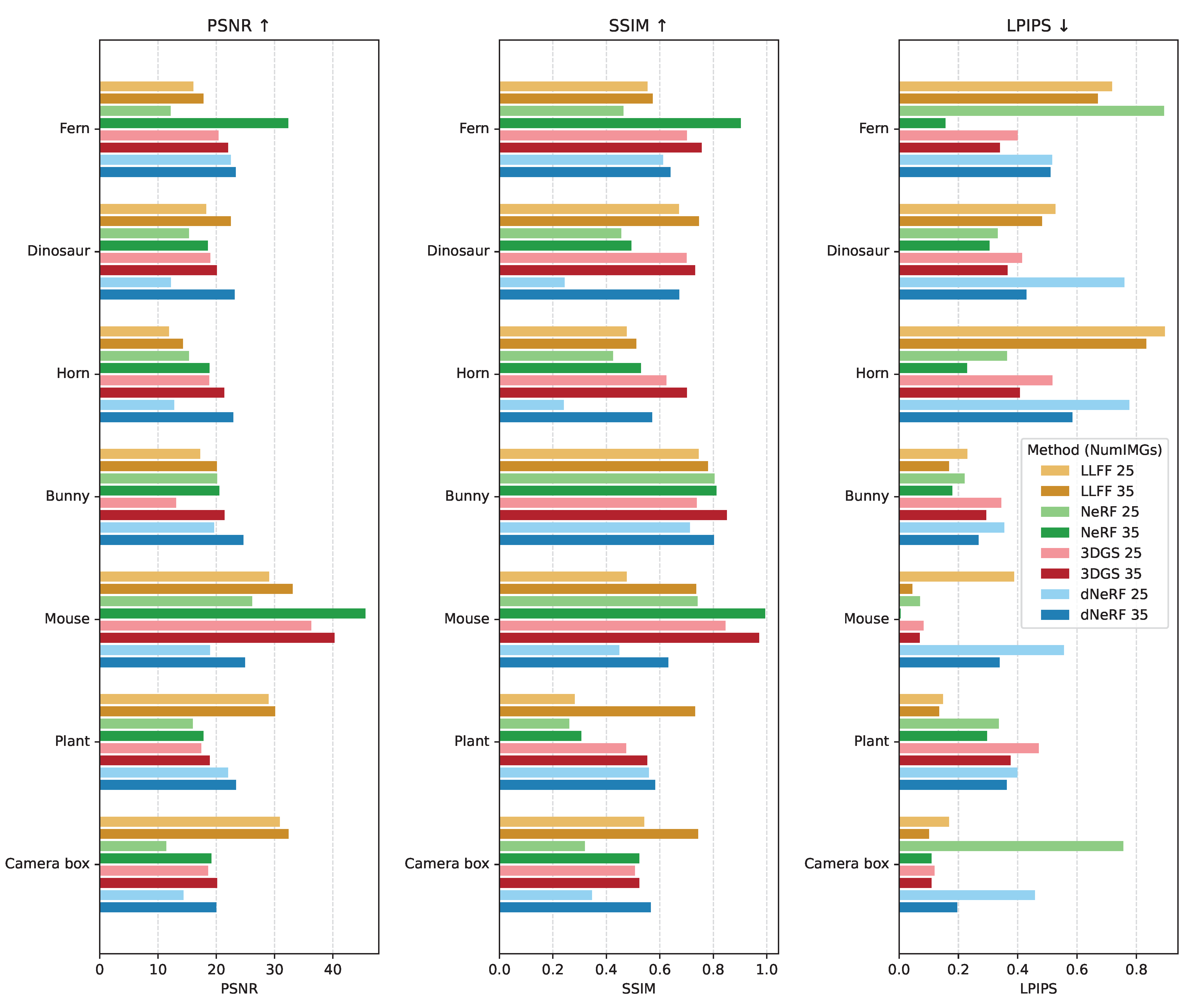
We evaluated 3D scene reconstruction quality using SSIM, PSNR, and LPIPS by comparing novel views rendered after training the model with 25 original images and with 35 images. Results are visualized in Figure 14. In the SSIM graph, the results for the 35-image dataset show a clear increase in SSIM values compared to those of the 25-image dataset, which is evident from the bars in the chart, and since higher SSIM indicates stronger structural similarity, this trend reflects improved reconstruction quality.

Similarly, in the PSNR graph, values for the novel views generated by the model after being trained with 35 images are higher, suggesting reduced noise and improved reconstruction quality. Since higher PSNR values indicate better quality, this shows the advantage of using 35 views.

In the LPIPS graph, the values for the novel views generated by the model after training with 35 images are lower than those obtained with 25 images, indicating greater perceptual similarity to the ground truth. Since lower LPIPS values reflect better perceptual similarity, this confirms that adding the extra generated novel views by our method improves the overall visual quality of the reconstructions.

These results suggest that the additional images in the 35-image dataset enhance structural accuracy, reduce noise, and increase perceptual resemblance, resulting in a more realistic and detailed reconstruction using the sparse light field method. The comparative analysis using the above-mentioned metrics confirms that the 35-image dataset consistently outperforms the 25-image dataset across all evaluation criteria, producing outputs that are not only structurally accurate but also visually and perceptually better. The additional views contribute significantly to more comprehensive, detailed, and reliable reconstructions.

6. Conclusions

The presented work introduces an innovative approach to overcoming the limitations of sparse light field data in 3D scene reconstruction by leveraging a hybrid CNN–LSTM framework with novel view synthesis based on interpolated as well as extrapolated camera poses. Our CNN–LSTM module is an upstream view densification stage for sparse captures. It does not replace existing technologies like NeRF/3DGS/LLFF. Instead, it synthesizes additional novel views at interpolated and extrapolated camera poses, which are then used to improve downstream reconstruction from sparse inputs. Evaluation is performed on held-out real images at real camera poses to avoid leakage, and synthesized views are never treated as ground truth unless a captured image exists at that pose.

By combining original and synthesized views, the method produces an enhanced dataset that improves the quality and completeness of 3D reconstructions. Experimental evaluations carried out with local light field fusion (LLFF), neural radiance fields (NeRFs), and 3D Gaussian Splatting (3DGS) confirmed that this enriched dataset yielded superior depth accuracy, structural consistency, and reduced artifacts compared to reconstructions using sparse inputs alone. Across all these methods, the measured metrics consistently validated the effectiveness of the proposed framework, further underlining its ability to generate realistic and high-fidelity scene representations.

A key contribution of this work is that it demonstrates the feasibility of employing an LSTM-based framework for novel view generation that has received little attention in the literature so far. This highlights a new research direction by showing that temporal modeling can be effectively exploited in light field enhancement. In addition, by enriching the dataset with synthesized views, the proposed method contributes to more complete and reliable 3D scene reconstructions. Nevertheless, it should be noted that the current framework relies solely on camera pose information as the conditioning variable, which may limit its ability to fully capture complex scene geometry.

Looking ahead, future work could explore integrating additional conditions, such as depth maps, semantic priors, or optical flow, to guide the synthesis process with richer scene information. We suggest that incorporating such modalities may improve geometric consistency and robustness, but this remains to be investigated. Furthermore, extending the framework to handle real-time or large-scale reconstructions could potentially broaden its applicability in practical systems. Additionally, the approach could help in more classical tasks like image stitching [34], where intermediate views could guide the keypoint matching process. Taken together, these directions outline promising avenues for advancing hybrid CNN–LSTM–based light field enhancement and 3D scene reconstruction technologies.