


Abstract
We forecast monthly Canadian real GDP growth using machine learning models trained on Official macroeconomic indicators and Google Trends (GT) data. Predictors are selected dynamically in each rolling window using PDC-SIS, with cross-validation-based tuning to support real-time forecasting and avoid data leakage. The evaluation is conducted on the latest-available (final-vintage) series and should be interpreted as a pseudo out-of-sample forecasting exercise rather than real-time vintage nowcasting. We evaluate GBM, XGBoost, LightGBM, CatBoost, and Random Forest against an ARIMA baseline. Official data deliver the strongest performance at short and medium horizons, while combining Official and GT data yields the clearest improvement at the longest horizon. With GT data alone, LightGBM is the only ML model maintaining positive out-of-sample R2 across all horizons. Diebold–Mariano tests corroborate these patterns: LightGBM dominates other ML models under GT-only predictors, whereas with Official and combined data, the horizon-specific best models significantly outperform ARIMA, with smaller differences among leading tree-based methods.
1. Introduction
Gross domestic product (GDP) is the primary measure for assessing the performance of an economy. It enables policymakers to judge whether the economy is expanding or contracting and permits them to make appropriate monetary or fiscal policy decisions accordingly. In this respect, the accurate and timely forecast of GDP growth ahead of the release of Official GDP figures is vital. Both quarterly and monthly GDP data are published with a two-month delay by Statistics Canada due to multiple revisions. Yet, some other Official macroeconomic information, such as employment, housing starts, and retail trades, often produced by national statistical bureaus, central banks, or other government institutions, are available much sooner in some cases, with only a few days’ delay. In addition, the use of Google Trends (GT) data for economic forecasting has become popular since the seminal work of Choi and Varian [1] and Choi and Varian [2]. GT data has been exploited to predict retail sales, automotive sales, home sales, and travel volume, among many others. GT allows users to download the time series data for a keyword search of particular interest in index form by selecting a specific geographic region and a specific time. Notably, Tkacz [3] used GT data to predict the 2008–2009 recession in Canada with a probit model, and observed an enormous surge in the search frequency of the word ‘recession’ about one month before the actual date of the 2008–2009 recession. In the context of GDP forecasting, Götz and Knetsch [4] used GT and other survey data to forecast German GDP with the Bridge regression. The Bridge regression has been used by policymakers to make short-term forecasts since at least the 1980s. Bridge models are linear dynamic models that use short-term indicators (available at a higher frequency) to forecast low-frequency variables such as aggregate GDP or its components. They obtained good forecasts when GT data was used instead of survey data (suggesting that GT data can be a good substitute for survey data when the latter are not available), but the forecast improvement tended to be smaller when both GT and survey data were used together. Ferrara and Simoni [5] also used a Bridge regression to nowcast Euro-area GDP with GT data. They employed Fan and Lv [6] Sure Independence Screening (SIS) to pre-select GT features as the first step. A Ridge regression was then used in the second step to construct forecasts given the pre-selected features. They then evaluated their forecasts using various combinations of data sources, and found GT data to be a useful predictor only before Official data become available.
In this paper, we apply state-of-the-art machine learning (ML) algorithms to forecast monthly Canadian GDP growth using both Google Trends (GT) and Official macroeconomic data from a large database of Fortin-Gagnon et al. [7]. We hereafter refer to the latter as Official data for the details of features selected by the RF model with PDC-SIS. Our approach introduces a novel dynamic feature selection methodology, which incorporates cross-validation in each rolling window. By dynamically pre-selecting relevant predictors in each rolling window, we ensure robust, up-to-date model adjustments, avoiding data leakage and enhancing real-time applicability.
For variable selection, short-term forecasts () rely primarily on high-frequency market and business indicators, with GT data capturing the automotive sector (Audi), small business trends, and electricity consumption, while Official data focus on residential mortgages, treasury bills, the stock exchange high, and energy exports. Medium-term forecasts () shift towards energy and employment indicators, with GT data emphasizing small business activity, electricity consumption, and rental market trends, and Official data highlighting WTI oil prices, energy exports, transportation imports, and employment services. For longer horizons (), industrial and labor market indicators become prominent, with GT data capturing finance sector activity, automotive trends (Volvo), and mining sector searches, while Official data focus on metal prices, consumer imports, manufacturing inventories, and total hours worked. At the very long-term (), structural economic indicators dominate, with GT data capturing agriculture sector activity, unemployment trends, and automotive searches (Volvo), while Official data emphasize energy exports, government bond spreads, consumer imports, and oil imports. Each dataset thus contributes distinct and complementary features across horizons, with electricity consumption from GT data and energy trade indicators from Official data maintaining consistent importance throughout all time frames.
We show that real GDP growth can be forecast accurately ahead of the release of GDP figures by using GT data and Official data variables as predictors. In particular, we investigate whether GT data remains useful for forecasting GDP when Official data are available. Most previous works on forecasting with GT data found this dataset to be useful when no Official data are available, and that its importance diminishes as soon as Official data become available (as in Götz and Knetsch [4] and Ferrara and Simoni [5]). Our results reveal that Official economic data consistently deliver the strongest forecasting performance at short and medium horizons, while combining Official and GT data achieves its clearest improvement only at the longest horizon. Official data produce the lowest RMSE at one, three, and six step horizons, demonstrating that traditional macroeconomic indicators provide robust predictive information. Combined data yield the lowest RMSE at the nine-step horizon, suggesting modest complementary benefits from GT variables at longer forecasts. GT data alone, however, produce substantially higher forecast errors than both Official and Combined approaches across all horizons, with most machine learning models failing to outperform the ARIMA baseline. These findings establish that Official economic indicators remain the primary source of predictive power for GDP forecasting, while GT data provide limited standalone value and modest incremental gains only when combined with Official data at specific horizons.Common Google Trends (GT) features selected by the Random Forest model with PDC-SIS are summarized in Table 1. Model performance proves data-source dependent rather than universal. For Official data, CatBoost achieves the lowest RMSE at short horizons, Random Forest at the medium horizon, and GBM at the long horizon. With GT data alone, LightGBM is the only ML model maintaining positive out of sample values across all horizons, while other ML models frequently underperform ARIMA. For combined data, CatBoost leads at short horizons, XGBoost at medium, and GBM at long horizons. Diebold–Mariano tests confirm these patterns: with GT data, LightGBM significantly outperforms all other ML competitors, while with Official and combined data, the best performing models at each horizon significantly outperform ARIMA at conventional significance levels, while differences among the leading tree-based models are often small. These results establish a clear data-source-specific model hierarchy: LightGBM for GT data, and CatBoost/Random Forest/GBM for Official and Combined data, depending on horizon. Rather than applying a single model universally, our findings underscore the importance of matching algorithms to data characteristics in macroeconomic forecasting applications.
Table 1.
Common Google Trends (GT) data features selected by the Random Forest model with PDC-SIS.
Work on forecasting with ML has recently been growing. Beyond macroeconomic forecasting, ML has also been widely applied to MOOC course recommendation, data-centric smart cities, and fraud detection in credit cards and blockchain-based financial systems [8,9,10,11]. It would be impossible to provide a complete list here. We shall unfortunately only be able to discuss a few, certainly not comprehensive, contributions that are closely related to the topic of the present paper. Biau and D’Elia [12] used the Random Forest (RF) algorithm to predict Euro-area GDP, and found that a combination of the RF and a linear model can outperform the benchmark autoregressive model. Other authors, such as Tiffin [13] and Jung et al. [14], have applied the Elastic Net, SuperLearner, and Deep Learning algorithms to produce forecasts that can outperform those made by traditional statistical methods. A comprehensive survey of applications of ML methods for macroeconomic forecasting is also provided by Fuleky [15]. Recently, Medeiros et al. [16] extensively applied standard ML methods to forecast the U.S. inflation rate, and found that the Random Forest (RF) algorithm can deliver the best forecasts among all the ML algorithms that they considered. Coulombe et al. [17] have shown that employing nonlinear models, regularization, cross-validation, and alternative loss functions can significantly improve the predictive performance of the ML methods in a data-rich environment. With respect to forecasts of Canadian GDP, Tkacz [18] adopted a neural network approach, while Chernis and Sekkel [19] used a dynamic-factors model. As the success of a supervised ML method depends on its capability to capture nonlinearities in the relationship between the response and predictive variables as well as in the (nonlinear) interactions between two predictive variables, in this study, we attempt to forecast Canadian GDP growth rate with (nonlinear) tree-based ensemble algorithms that have not been fully explored for economic forecast, namely, eXtreme Gradient Boosting (XGBoost), CatBoost and Microsoft’s Light Gradient Boosting Machine (LightGBM). For example, XGBoost by default utilizes a nonlinear booster, gbtree; however, one can use the linear booster gblinear to generate linear models. Such ensemble methods have demonstrated empirical success in many applications, as averaging several nonlinear models with potentially different sets of predictive variables is often an effective way to address model uncertainty, which is very common in practice (see, e.g., Athey et al. [20]).
While comparing the methodology of various papers, we focus on four dimensions: (i) how predictors are chosen (external screener versus embedded penalties/factors/Bayesian inclusion); (ii) where and how hyperparameters are tuned (nested or joint procedures versus sequential choices); (iii) the window structure (rolling versus expanding/recursive); and (iv) whether the design is leakage-safe in real time. Closest to our setting is Ferrara and Simoni [5], who implement a sequential, within-date procedure: they first conduct a targeted preselection of Google Search Data conditional on official indicators (t-stat/SIS-style screening calibrated by asymptotic thresholds), and then estimate a ridge regression on the screened set with the penalty chosen by generalized cross-validation. Estimation is performed in pseudo-real-time using real-time vintages and an expanding (recursive) sample across weekly within-quarter information sets; there is no use of PDC–SIS and no tree-boosting learners. Methodologically related but distinct are the following strands. Bulligan et al. [21] create “targeted predictors” by screening across many estimation windows and then fix the feature pool before the out-of-sample period (i.e., no re-selection in each forecast window). Babii et al. [22] and Beyhum and Striaukas [23] employ penalized MIDAS specifications with blocked cross-validation, where selection is embedded in the penalty rather than performed by an external screener. Soybilgen and Yazgan [24] extract dynamic factors from large monthly panels and feed those factors to bagging, Random Forests, and Gradient Boosting with tuning performed once rather than in every window. Kant et al. [25] compare machine-learning methods for Dutch GDP in expanding windows with per-forecast cross-validation and embedded selection. Franjic and Schweikert [26] combine Elastic-Net preselection with dynamic factor models in rolling windows.
Compared with Bayesian dynamic-inclusion models in the econometric tradition—which endogenize selection via state-space priors and variational Bayes—our contribution is a practical ML pipeline that dynamically screens with PDC–SIS and conducts tuning and estimation within each rolling window for real-time deployment. Our approach also differs from recent high-dimensional forecasting methods in two key respects. First, whereas Babii et al. [22] embed variable selection within penalized linear regression (sparse-group LASSO), we perform explicit distance-correlation screening (PDC–SIS) to capture nonlinear predictor–target dependence before applying tree-based ML. Second, we integrate PDC–SIS screening, hyperparameter tuning, and model estimation inside a single rolling-window pipeline, using only data available in each window. This one-step, leakage-safe framework enables the use of nonlinear ensemble methods (GBM, XGBoost, CatBoost, and Random Forest)—which do not possess built-in selection mechanisms—while preserving strict temporal separation. Relative to Franjic and Schweikert [26], who combine Elastic Net with factor models, our framework (i) uses PDC–SIS to capture nonlinear dependence beyond linear penalties, (ii) employs tree-based ML rather than factor structures, and (iii) is model-agnostic and thus applicable to any learner. Building on our previous work applying distance-correlation screening with machine-learning models for GDP forecasting Chu and Qureshi [27], this study introduces the first dynamic implementation in which the screening is performed adaptively within each rolling window. To our knowledge, this is the first application of distance-correlation screening for adaptive feature selection in macroeconomic forecasting with nonlinear ensemble methods, executed within a one-step rolling-window pipeline and evaluated head-to-head across Official, Google Trends, and combined data at multi-month horizons.
Our proposed forecasting procedure is a one-step procedure detailed in Section 3. This streamlined approach integrates variable selection and forecasting into a single, continuous process. We employ Yousuf and Feng [28]’s distance-correlation-based variable screening procedure, namely the PDC-SIS, to dynamically select the most relevant predictors within each rolling window. We use the standard forecast evaluation metrics: the root mean squared error (RMSE), the mean absolute error (MAE), the mean absolute deviation (MAD), and OoS .
The rest of this paper is outlined as follows: Section 2 provides a brief description of the ML algorithms employed in this paper. Although this description may appear non-technical, interested readers can find a rigorous treatment of these algorithms in many good ML textbooks, for example, Hastie et al. [29] and Murphy [30]. Section 3 details the forecasting procedure, implemented in two operational steps. Section 4 presents GT and Official data that we used to predict GDP growth rate. Section 5 provides the main empirical findings of this paper. Section 6 concludes this paper. Finally, further details about the software packages used to implement the ML methods and other tables and figures are collected in two appendices at the end of the paper.
2. Description of ML Algorithms
This section briefly summarizes the learning algorithms used in our forecasting exercise, focusing on the elements that are relevant for replication and interpretation in a rolling real-time design. For a general background on tree-based learners and boosting, we refer the reader to standard texts (e.g., Murphy [30], Chapter 16) and the original methodological papers cited below.
2.1. Decision Trees (Building Block)
Tree-based methods approximate the conditional mean by recursively partitioning the predictor space into regions and assigning a constant prediction to each region (leaf). In regression settings, split points are chosen greedily to reduce a loss such as the sum of squared errors within leaves. Because unconstrained trees can overfit, practical implementations control tree complexity through hyperparameters such as maximum depth, minimum leaf size, and the minimum number of observations required to split a node. These complexity controls are selected within each rolling window as part of our tuning protocol (see Section 3).
2.2. Random Forests (Bagging-Based Ensemble)
Random Forests, proposed by Breiman [31] reduce the variance of a single tree by averaging predictions across many decorrelated trees trained on bootstrap samples and random subsets of predictors at each split. In our application, the main tuning dimensions are the number of trees and the parameters governing tree complexity (depth/leaf size) and feature subsampling. Averaging across trees yields robust performance in data-rich settings and mitigates overfitting relative to a single deep tree.
2.3. Gradient Boosting and Boosted-Tree Variants
Boosting constructs an additive model by fitting weak learners sequentially, where each new tree is chosen to reduce a loss function given the current ensemble Freund and Schapire [32], Breiman [33], Friedman [34]. In Gradient Boosting, the next tree is fit to the negative gradient of the loss (often interpreted as residual-like information under squared-error loss). Key regularization mechanisms include shrinkage (learning rate), limiting tree depth, and row/column subsampling. These controls govern the bias–variance trade-off and are tuned within each rolling window.
We evaluate several boosted-tree implementations. XGBoost [35] augments Gradient Boosting with explicit regularization terms and efficient split finding, often improving generalization and computational speed. LightGBM and CatBoost follow the same boosted-tree principle but differ in engineering choices (e.g., histogram-based splitting, growth policies, and handling of categorical features), which can materially affect performance in large, sparse, or mixed-type predictor sets. Across boosted-tree methods, the main tuned hyperparameters include the number of boosting iterations, learning rate, maximum depth (or leaf constraints), subsampling rates, and regularization strength.
2.4. Why Tree-Based Ensembles Are Suitable Here
Tree-based ensembles (RF and boosted trees) are attractive for macro-forecasting with many candidate predictors because they can accommodate nonlinearities and interactions without requiring explicit functional-form specification. Moreover, with appropriate regularization and a strict rolling-window training/validation protocol, these methods can provide stable out-of-sample performance in high-dimensional environments. Any additional implementation details (e.g., exact tuning grids and validation design) are provided in the methodology section to avoid redundancy.
3. Forecasting Method
Following Chu and Qureshi [27], we employ a recursive rolling-window strategy to evaluate the out-of-sample (OoS) performance of our forecasting models over time. Multiple rolling sub-samples are constructed by shifting the window forward by one observation, thereby incorporating the most recent data available while discarding the oldest observation. For each sub-sample, we compute the OoS performance metrics (RMSE, MAD, MAE, and OoS ) for different forecast horizons (), preserving a real-time forecasting context by avoiding the use of future information in the modeling process.
Variable selection is dynamically performed within each rolling window, ensuring that the model continuously adapts to the most relevant predictors as new data becomes available, effectively preventing data leakage. In each rolling sub-sample, the data is split into three segments for training, validation, and evaluation. Each rolling sub-sample maintains fixed sizes for these segments: the training set consists of the initial portion of observations, followed by a validation set of 16 observations, and finally, an evaluation segment used to produce -step-ahead forecasts. The training set size varies depending on the forecast horizon, ensuring that the overall sub-sample size () remains consistent. For instance, with , a one-step-ahead forecast () uses 81 observations for training, whereas a nine-step-ahead forecast () uses 65 observations for training. This structure supports forecasts for one- to nine-period-ahead horizons and ensures consistency across all rolling windows. The tuning spaces used for all ML algorithms are reported in Appendix A, Table A4. The rolling-window forecasting scheme is illustrated in Figure 1. We refer to this as a one-step procedure because variable selection, hyperparameter tuning, and estimation are executed together within each rolling window. In each rolling window, we split the data into training, validation, and evaluation segments. Variable selection is performed dynamically using PDC-SIS on the training segment only, ensuring that only information available up to that window is used and preventing any future information from influencing selection. Conditional on the selected predictors, we tune hyperparameters on the validation segment by selecting the configuration that minimizes out-of-sample (OoS) RMSE. The model is then refit on the combined training and validation segments using the selected predictors and optimal hyperparameters, and it generates -period-ahead forecasts for the evaluation segment as the window rolls forward. Each realized observation, aligned with the forecast horizon, is subsequently used to compute forecast errors.
Figure 1.
Rolling-window forecasting scheme. Each rolling window is split into training, validation, and test segments, and the window then moves forward through time.
We use data from January 2004 to September 2021, totaling 214 months, as January 2004 is the earliest date for which Google Trends (GT) data is available. Although recent data retrieval is limited by API rate limits and associated costs, we previously downloaded historical GT data to ensure comprehensive analysis and consistency across time. For both Official and GT data, we apply a first-difference transformation to the logarithmic values of the variables and scale these values by multiplying by 100. This transformation standardizes the data for analysis. Additionally, we performed the Kwiatkowski–Phillips–Schmidt–Shin (KPSS) test to confirm stationarity of the transformed variables, verifying that all variables are indeed stationary.
We evaluate forecasts using four metrics: the root mean squared error (RMSE), mean absolute error (MAE), median absolute deviation (MAD), and out-of-sample (OoS ). Let denote the -step-ahead forecast error of model m. For each horizon , we compute rolling-window accuracy measures over a window of length W:
For the OoS , we use the rolling RMSE-ratio definition reported in our empirical results. Let denote the benchmark forecast, computed as a backward-looking rolling mean of past realizations using a window of length B. Define the benchmark rolling RMSE analogously. The rolling OoS is:
In contrast, ARIMA is used as the baseline model comparator for the forecast evaluations (and the Diebold–Mariano tests); the rolling-mean benchmark is used only for constructing OoS .
We summarize rolling performance by reporting the median and interquartile range (IQR) of , , , and across the out-of-sample evaluation period.
The out-of-sample (OoS ) takes values in . Negative values indicate that the benchmark forecast has lower rolling RMSE than the model, while positive values indicate that the model improves upon the benchmark in rolling RMSE. Values closer to one imply greater predictive accuracy relative to the benchmark.
For each metric (RMSE, MAE, and MAD), our objective is to minimize deviations between predictions and observations, thus obtaining the smallest possible values for these metrics given our choice of predictors, . These metrics collectively provide a quantitative measure of the success of our predictions.
4. Data
Official data: The Official dataset includes Canadian economic variables dynamically selected for each forecast horizon and step from a large monthly database by Fortin-Gagnon et al. [7]. Using PDC-SIS for variable selection, relevant predictors are chosen based on their predictive power at each forecast step. Common variables selected across multiple horizons by the Random Forest model include the Toronto Stock Exchange high, six-month Treasury bills, Government bonds (1–3, 3–5, and 5–10 years), WTI crude oil price, IPPI (metal and machinery), Export energy products, Export oil, Import consumption goods, Residential mortgages, New housing price index, Employment services, Total employment, Total hours worked, and Manufacturing inventories. The variables used to predict monthly real GDP growth rates are summarized in Table 2.
Table 2.
Common Official data selected by the Random Forest model with PDC-SIS.
GT data: This dataset is available at www.google.com/trends provides all search volumes and shows the percentage of web searches performed on Google. GT dataset reports data in terms of an index of queries rather than in terms of the raw number of queries. This index is then normalized so that the maximum search volume at a given point in time and location is set to 100%, and every other observation is calculated relative to that maximum value. The resulting numbers on the scale from zero to 100 are thus based on the total number of searches for a specific category relative to all other search queries. To address the well-documented sampling variation in Google Trends data, we follow the methodology proposed by Eichenauer et al. [36]. Specifically, we download multiple random samples of GT data at different periods and average the series to reduce sampling noise. This approach produces more consistent and reliable time series, mitigating the randomness inherent in Google’s sampling procedure.
Google Trends indices are based on Google’s sampling and normalization and may vary across downloads even when the same query settings are used. For transparency, our replication package archives the processed Google Trends panel used in estimation (after cleaning and seasonal adjustment), together with scripts documenting query settings (e.g., geography, category, time window, and term lists) and download dates recorded at the day level (YYYY–MM–DD). Consequently, the reported results are computationally reproducible from the archived data and code, while exact reconstruction by re-downloading raw Google Trends series from the public interface may not be perfectly identical.
Choi and Varian [1] have used the term “Google Trends” while Götz and Knetsch [4] and Ferrara and Simoni [5] have used the term “Google search data”. GT data is an unbiased sample of the Google search data. According to the Canadian internet usage survey in 2018, 94% of the population had internet access at home, and the share of all the Canadians aged 15 or above who used the internet was 91%. Interestingly, approximately 84% of the internet users bought about $57.4 billion worth of goods or services online in 2018 compared to $18.9 billion in 2012. GT data are only available for normal users from January 2004 to date.
We divided our GT dataset into two primary categories. The search keywords in the first category, which we term general search terms, were obtained through the R package gtrendsR (see Table 3). This initial set included 26 categories and 269 subcategories, yielding a total of 1776 search terms. Only 464 search terms remain after removing columns with missing values and outliers. The second category, referred to as relevant search terms, includes variables that directly align with the monthly and quarterly components of Canadian GDP (see Table 4). This category comprises 80 search terms. For variables in the second category with minimal missing values, we replaced up to two missing entries with the column mean. Following a thorough screening process that involved removing columns with missing values, filtering outliers, and careful manual selection for relevance, 37 search terms were retained.
Table 3.
Google Trends (GT) general search terms.
Table 4.
Google Trends (GT)-customized search keywords (relevant search terms).
The manual relevance screen retained terms only if they had a clear link to Canadian aggregate activity (GDP components and/or industries represented in the monthly GDP accounts) and a stable interpretation over time. Terms were excluded if they were ambiguous in meaning, primarily non-economic in context, event-driven/one-off, or exhibited excessive missingness or unstable spikes inconsistent with broad economic activity. Importantly, this screening was conducted without reference to GDP outcomes or model performance.
Additionally, we applied the X-13ARIMA-SEATS program, developed by the U.S. Census Bureau and the Bank of Spain, to seasonally adjust GT data, ensuring consistency for use in economic forecasting.
5. Empirical Results
5.1. Selection of Predictors
In our approach, dynamic feature selection is applied in each rolling window at each forecast horizon, resulting in a diverse set of predictors tailored to the model’s needs at each step. Given the complexity and volume of selected features, it is nearly impossible to present every feature used across all windows and horizons. Therefore, we focus on the features that were consistently selected across windows by PDC–SIS within each dataset, which allows us to highlight the most impactful variables in a manageable format. Therefore, we focus on the features that were consistently selected across windows by PDC–SIS within each dataset, which allows us to highlight the most impactful variables in a manageable format. For comparability, Table 1, Table 2 and Table 5 report these consistently selected predictors using Random Forest as a fixed reference implementation.
Table 5.
Common GT plus Official features selected by Random Forest with PDC-SIS.
5.2. Official Data
In the case of Official data, model leadership varies by horizon: CatBoost leads at short horizons (), Random Forest at the medium horizon (), and GBM at the long horizon (). The predictors selected by PDC-SIS reveal distinct patterns across forecast horizons (see Table 2). In the short term (), forecasts rely heavily on credit and market variables, such as residential mortgages, treasury bills, stock exchange high, and energy exports, which capture immediate economic fluctuations. For medium-term horizons (), energy and employment variables, like WTI oil prices, energy exports, transportation imports, and employment services, gain prominence, reflecting the influence of global energy markets and labor conditions on economic activity. In longer-term forecasts ( and ), industrial production and trade indicators dominate, with metal prices, manufacturing inventories, consumer imports, and government bond spreads highlighting the role of industrial activity and monetary policy in sustaining economic growth over time.
5.3. GT Data
In the case of GT data, LightGBM is the top-performing model. The features selected by PDC-SIS for the GT dataset display unique trends across forecast horizons (see Table 1). Short-term predictions () rely heavily on automotive sector searches (Audi), small business trends, and electricity consumption, reflecting immediate economic activity in consumer and business sectors. Defense sector indicators (Army) show strong persistence across short and medium horizons, suggesting their sustained relevance in economic forecasting. Financial indicators, including loan and finance sector activity, gain prominence in longer horizons (), highlighting the role of credit conditions in medium-term growth. Meanwhile, at very long horizons (), automotive searches shift to Volvo and Ford, with insurance, unemployment, and agriculture sector activity becoming increasingly important in capturing structural economic trends.
5.4. Combined GT and Official Data
The combined analysis of GT and Official data highlights distinct feature patterns across forecast horizons (see Table 5). According to the forecasting results, CatBoost leads at short horizons (), XGBoost at the medium horizon (), and GBM at the long horizon (). In the short term (), forecasts rely heavily on consumer behavior and financial indicators, with Google Trends capturing automotive sector activity (Audi), small business trends, and electricity consumption, while Official data emphasize residential mortgages, treasury bills, stock exchange high, and energy exports. As the horizon extends to the medium term (), a shift occurs toward energy and labor market indicators, with Google Trends focusing on small business trends, electricity consumption, and rental market activity, while Official data highlight WTI oil prices, energy exports, transportation imports, and employment services.
For longer horizons (), industrial and finance indicators gain importance, such as finance sector searches, automotive trends (Volvo), and mining sector activity in Google data, complemented by metal prices, consumer imports, manufacturing inventories, and total hours worked in Official data. In the very long term (), structural economic indicators become dominant, with Google Trends showing agriculture sector activity alongside unemployment and automotive searches (Volvo), while Official data emphasize energy exports, government bond spreads, consumer imports, and oil imports. This evolution across time horizons demonstrates how high-frequency Google Trends data combined with fundamental Official indicators allows short-term forecasts to align with immediate market conditions and consumer behavior, while long-term forecasts increasingly capture structural economic factors and monetary policy indicators. Notably, small business trends and real estate activity in Google data maintain importance across all time horizons, suggesting their persistent relevance as economic barometers, while Official data show a clear progression from immediate market indicators toward broader monetary and inflation measures as the forecast horizon extends.
Yousuf and Feng [28]’s variable screening procedure based on Székely and Rizzo [37]’s partial distance correlation, namely PDC-SIS, can be used to select time-series variables. This procedure defines the set of possible predictors as
for and where K is the number of features and L is a maximum number of lags to be set. Using the partial distance correlation to screen out irrelevant variables has an important advantage over the conventional partial correlation, as a null partial distance correlation between two variables implies conditional independence between these two variables, while this is not necessarily the case with other measures of conditional correlation. Therefore, if an element in the set of predictors has zero partial distance correlation with the target variable, then this element has no predictive ability power. All the ML algorithms used in this paper actually train nonlinear models in which features and the target variable may have complex relationships. PDC-SIS can effectively select predictors that can be either linearly or nonlinearly associated with the target variable.
5.5. Comparison of Forecasts
Given the set of predictors selected in Section 5.1 above, we proceed with the sliding-window forecasting strategy described in Section 3. The following ML algorithms were implemented: Random Forest, Gradient Boosting Machine (GBM), CatBoost, Light Gradient Boosting Machine (LightGBM), and XGBoost described in Appendix A. We include an ARIMA model as the baseline comparator for forecast evaluation (including Diebold–Mariano tests). In addition, for constructing OoS , we use a simple rolling-mean benchmark, defined as the historical average of past GDP growth computed over a fixed-length backward-looking window. Our analysis reveals that no single data source or model dominates across all forecast horizons, with performance varying systematically by both horizon and data source.
We multiply the median of all metrics by 100 for better visibility, excluding OoS . The GT data is available from 2004 to 2021, so for a better comparison, we used Official datasets from 2004 to 2021. All the forecasts of the monthly GDP growth rate using both official and GT data for a period (the entire sample period for the Official data and GT is from January 2004 to September 2021, and the out-of-sample period is from August 2012 to September 2021 for Official and GT) are presented in Table 6, Table 7 and Table 8.
Table 6.
Official data variable selection with PDC-SIS: Forecast evaluation using the median of rolling out-of-sample (OoS) RMSE, MAE, and OoS with a window size of 75 months (August 2012 to September 2021; full sample: 2004–2021).
Table 7.
GT data variable selection with PDC-SIS: Forecast evaluation using the median of rolling out-of-sample (OoS) RMSE, MAE, and OoS with a window size of 75 months (August 2012 to September 2021; full sample: 2004–2021).
Table 8.
Official + GT data variable selection with PDC-SIS: Forecast evaluation using the median of rolling out-of-sample (OoS) RMSE, MAE, and OoS with a window size of 75 months (August 2012 to September 2021; full sample: 2004–2021).
The first column of the table presents the different forecast horizons, while the second column lists the performance metrics, including RMSE, MAE, and OoS . The remaining columns show the median values of rolling RMSE, and MAE for each machine learning algorithm, with variable selection conducted using the PDC-SIS method. Beneath each median value, dispersion is reported using the interquartile range (IQR), which represents the difference between the first and third quartiles. A model with either a lower median RMSE or MAE or MAD, or a lower IQR, is considered to have better performance.The rolling RMSE and MAE for Official data (2004–2021), and Official plus GT data and Google Trends data, are shown in Figure 2, Figure 3 and Figure 4. A boxplot shows the five-number summary of a set of data: the minimum value, first quartile (25 percent), median, third quartile (75 percent), and maximum values. Using a vertical number line and a rectangular box to build a box plot, the minimum and maximum values are the endpoints of the axis. The first quartile displays one end of the box, and the third quartile the other end of the box. The box shows the interquartile range, where a horizontal line goes through the box at the median or second quartile. The outliers are displayed outside the whisker (the whiskers are the two lines outside the box). Here are the key takeaways:
Figure 2.
Rolling out-of-sample RMSE and MAE for different forecast horizons using PDC-SIS variable selection with official data. Note: The left panel shows the rolling RMSE and the right panel shows the rolling MAE for different forecast horizons () using PDC-SIS variable selection with Official data.
Figure 3.
Rolling out-of-sample RMSE and MAE for different forecast horizons using PDC-SIS variable selection with GT data. Note: The left panel shows the rolling RMSE and the right panel shows the rolling MAE for different forecast horizons () using PDC-SIS variable selection with GT data.
Figure 4.
Rolling out-of-sample RMSE and MAE for different forecast horizons using PDC-SIS variable selection with GT plus Official data. Note: The left panel shows the rolling RMSE and the right panel shows the rolling MAE for different forecast horizons () using PDC-SIS variable selection with GT plus Official data.
- Higher Accuracy with Combined Data:Table 6, Table 7 and Table 8 show that combining Official + GT data delivers competitive accuracy at short horizons with the clearest gain emerging at the long horizon, while Official data alone remain best at short and medium horizons. At , the best Official model is CatBoost with median RMSE (Table 6), marginally lower than the best combined-data RMSE (CatBoost, Table 8) and substantially lower than the best GT-only RMSE (LightGBM, Table 7). At , Official again dominates (CatBoost: , Table 6) relative to combined ( by CatBoost, Table 8) and GT-only ( by LightGBM, Table 7). At , Official delivers the lowest RMSE (Random Forest: , Table 6), with combined close behind ( by XGBoost, Table 8), while GT-only remains substantially higher ( by LightGBM, Table 7).The clearest benefit from combining data emerges at , where combined achieves the lowest RMSE overall ( by GBM, Table 8) versus Official ( by GBM, Table 6) and GT-only ( by LightGBM, Table 7). In terms of out-of-sample (defined relative to the rolling-mean benchmark in Equation (4)), Official data remain consistently strong across all horizons (Table 6). GT-only shows substantially weaker performance, with most models registering negative OoS ; only LightGBM and ARIMA maintain positive values across horizons (Table 7). The combined dataset achieves its highest OoS at (CatBoost: , Table 8), exceeding Official data’s best at this horizon (RF: , Table 6).
- Official Data Performance:Official data (Table 6) deliver the strongest and most consistent accuracy profile overall, with positive OoS at all horizons for all machine learning models. By RMSE, the best models are CatBoost at () and (), Random Forest at (), and GBM at (). By out-of-sample (relative to the rolling-mean benchmark in Equation (4)), Random Forest achieves the highest values across most horizons: at (ARIMA’s out-of-sample is ), at (ARIMA’s out-of-sample is ), and at (ARIMA’s out-of-sample is ), while GBM leads at with (ARIMA’s out-of-sample is ). Diebold–Mariano tests (Table 9) confirm CatBoost’s superiority at and 3, Random Forest’s at , and GBM’s at , with the leading model significantly outperforming ARIMA at each horizon.Table 9. Diebold–Mariano Test Results (Official Data): Pairwise forecast accuracy comparisons. Model 1 shows significantly better performance than the listed Model 2 competitors.
- GT Data Effectiveness:GT data alone (Table 7) yield materially higher forecast errors than Official or combined data and exhibit substantially weaker overall fit, with most models failing to outperform the ARIMA baseline model. LightGBM emerges as the most consistent GT-only performer, achieving the lowest RMSE at all horizons: (), (), (), and (), compared to ARIMA’s and , respectively. Most non-(LightGBM/ARIMA) models register negative OoS , while LightGBM maintains modest positive values across horizons: at (vs. ARIMA’s ), at (vs. ), at (vs. ), and at (vs. ARIMA’s ). Diebold–Mariano tests (Table 10) confirm LightGBM’s statistical dominance across all horizons, significantly outperforming all ML competitors.Table 10. Diebold–Mariano Test Results (GT Data): Pairwise forecast accuracy comparisons. Model 1 shows significantly better performance than the listed Model 2 competitors.
- Combining GT with Official Data:Table 8 demonstrates that combining GT with Official data is competitive at short horizons and provides the clearest RMSE improvement at the long horizon, though the gains are often statistically indistinguishable from Official data alone. By RMSE, the best combined-data models are CatBoost at () and (), XGBoost at (), and GBM at (). In terms of OoS (relative to the rolling-mean benchmark in Equation (4)), combined data achieve the strongest performance at where CatBoost attains (ARIMA’s out-of-sample is ), exceeding Official data’s best of (RF, Table 6). At , CatBoost achieves (vs. ARIMA’s ), at , XGBoost reaches (vs. ), and at , GBM attains (vs. ). While the combined dataset achieves the lowest absolute RMSE at (), Official data maintain higher OoS values at and 9 (Table 6 vs. Table 8). Diebold–Mariano tests (Table 11) confirm the best models’ superiority: CatBoost at and 3, XGBoost at , and GBM at , with leading models significantly outperforming ARIMA.Table 11. Diebold–Mariano Test Results (Official + GT Combined Data): Pairwise forecast accuracy comparisons. Model 1 shows significantly better performance than the listed Model 2 competitors.
- Model Performance Comparison Across Forecast Horizons:Model dominance proves primarily data-source-specific rather than universally stable across datasets. For Official data (Table 6), tree-based ensemble methods dominate: CatBoost leads by RMSE at short horizons ( and 3), Random Forest at the medium horizon (), and GBM at the long horizon (). For GT data (Table 7), LightGBM is the sole consistent performer, achieving the lowest RMSE at all horizons and (alongside ARIMA) generating the only positive OoS results. For combined data (Table 8), RMSE leaders mirror the Official pattern at short horizons (CatBoost at and 3), shifting to XGBoost at , and to GBM at . Diebold–Mariano tests (Table 9, Table 10 and Table 11) confirm the statistical significance of the RMSE rankings, and Table 12 consolidates the horizon-specific winners across data sources. LightGBM dominates with GT data across all horizons, while with Official and combined data, CatBoost leads at short horizons and different models excel at longer horizons, with the leading model significantly outperforming ARIMA at each horizon.Table 12. Diebold–Mariano Test Summary: Best performing models by data source and forecast horizon.
- Stability Analysis Using IQR Metrics:The interquartile ranges (values in parentheses) reveal that GT-only forecasts exhibit substantially higher variability across rolling windows than Official or combined data at all horizons. At RMSE, Official CatBoost displays IQR (Table 6), and combined CatBoost is marginally tighter with IQR (Table 8), while GT LightGBM shows higher dispersion with IQR (Table 7). This pattern persists across horizons: at RMSE, the combined best model (XGBoost: IQR , Table 8) proves more stable than GT LightGBM (IQR , Table 7). Similar patterns emerge in OoS metrics, where GT models display wider IQR spreads than Official or combined counterparts. The elevated variability in GT forecasts underscores the challenges of forecasting with search-based indicators: despite LightGBM’s consistent RMSE advantage, the higher rolling-window variance in GT data reflects greater instability in the underlying signal.
A more detailed analysis of Table 6, Table 7 and Table 8 also permits a comparison of the predictive success of models depending on the different forecast horizons and different datasets.
One-step-ahead forecasts: Models trained on Official data (Table 6) show strong positive OoS values across all models, with RF achieving 0.3282, followed by GBM at 0.3221 and CatBoost at 0.3138. CatBoost achieves the lowest RMSE of 0.2729, closely followed by GBM at 0.2747. In contrast, GT data alone (Table 7) produces weak performance, with LightGBM achieving the lowest RMSE of 0.3008 and a modest OoS of 0.0755, while most other models show negative OoS values. For the combined dataset (Table 8), performance improves notably: CatBoost achieves the highest OoS of 0.3366 and lowest RMSE of 0.2733, followed by GBM (OoS 0.3040, RMSE 0.2747). These results confirm that combining Official and GT data yields competitive short-term forecasting performance, with the combined dataset achieving the highest OoS observed. Diebold–Mariano tests (see Table A1, Table A2 and Table A3 in Appendix A for complete pairwise results) reveal distinct patterns across data sources. For Official data, CatBoost significantly outperforms LightGBM and ARIMA at the 1% level, while showing no significant differences versus GBM, XGBoost, or RF, indicating these top models are statistically tied despite CatBoost’s lower average RMSE. For GT data, LightGBM significantly outperforms all ML competitors at the 1% level (except RF at the 5% level), while maintaining statistical parity with ARIMA. For Combined data, CatBoost significantly beats LightGBM and ARIMA at the 1% level, mirroring the Official data pattern.
Three-steps-ahead forecasts: Official data maintains strong predictive accuracy (Table 6), with CatBoost achieving the lowest RMSE of 0.2643 and OoS R2 of 0.2621, followed by XGBoost (RMSE 0.2699, OoS R2 0.2689) and RF (RMSE 0.2712, OoS R2 0.2782). For GT data alone (Table 7), LightGBM performs best with a RMSE of 0.3021 and OoS R2 of 0.0821, while most other models show negative or near-zero out-of-sample values. The combined dataset (Table 8) shows CatBoost leading with a RMSE of 0.2688 and OoS R2 of 0.1545, followed by XGBoost (RMSE 0.2709, OoS R2 0.1618). Diebold–Mariano tests (Table A1, Table A2 and Table A3) show CatBoost’s strongest dominance at this horizon. For Official data, CatBoost significantly outperforms all competitors at conventional significance levels: most at the 1% level, with RF at the 10% level. For GT data, LightGBM significantly outperforms all four ML competitors at the 1% level, demonstrating complete statistical superiority. For Combined data, CatBoost significantly beats GBM at the 5% level, and LightGBM and ARIMA at the 1% level, though it shows no separation from XGBoost or RF.
Six-steps-ahead forecasts: Official data continue to deliver strong performance (Table 6), with RF achieving the lowest RMSE of 0.2603 and highest OoS R2 of 0.3177, followed by XGBoost (RMSE 0.2616, OoS R2 0.2988) and CatBoost (RMSE 0.2688, OoS R2 0.2875). For GT data alone in Table 7, LightGBM maintains its lead with a RMSE of 0.3026 and OoS R2 of 0.0897, while other models show substantially weaker performance with negative OoS R2 values. The combined dataset (Table 8) shows XGBoost achieving the lowest RMSE of 0.2616 with an OoS R2 of 0.2588, followed by RF (RMSE 0.2637, OoS R2 0.2733). Diebold–Mariano tests (Table A1, Table A2 and Table A3) reveal data-source-dependent patterns. For Official data, RF significantly outperforms LightGBM and ARIMA at the 1% level, while showing no significant differences versus GBM, XGBoost, or CatBoost. For GT data, LightGBM achieves complete dominance, significantly outperforming all ML competitors at the 1% level. For Combined data, XGBoost marginally outperforms GBM at the 10% level and significantly beats LightGBM and ARIMA at the 1% level, with no significant differences versus CatBoost or RF.
Nine-steps-ahead forecasts: At the longest horizon, Official data shows GBM achieving the lowest RMSE of 0.2722 with an OoS R2 of 0.2695 (Table 6), followed by XGBoost (RMSE 0.2795, OoS R2 0.2400). For GT data alone (Table 7), LightGBM continues its consistent performance with a RMSE of 0.3020 and OoS R2 of 0.0891, while other models deteriorate substantially. The combined dataset (Table 8) achieves the lowest overall RMSE across all specifications at this horizon: GBM records 0.2710 with an OoS R2 of 0.1822, closely followed by XGBoost (RMSE 0.2782, OoS R2 0.2171). Diebold–Mariano tests (Table A1, Table A2 and Table A3) show convergence to statistical parity among top ML models at the longest horizon. For Official data, GBM marginally outperforms LightGBM at the 10% level and significantly beats ARIMA at the 1% level, with all other ML models statistically tied. For GT data, LightGBM maintains its dominance, significantly outperforming all four ML competitors at the 1% level. For Combined data, GBM significantly outperforms only ARIMA at the 1% level, with all ML models showing no significant differences among themselves, indicating comparable long-horizon performance.
In summary, our comprehensive analysis reveals robust machine-learning superiority over the ARIMA baseline model in RMSE-based evaluations and Diebold–Mariano tests when using Official economic data; additionally, all models achieve positive out-of-sample relative to the rolling-mean benchmark (Equation (4)) across horizons. Official data consistently deliver the strongest performance at short and medium horizons, while the combined Official and GT dataset achieves the highest short-horizon OoS R2 (0.3366 at ) and lowest long-horizon RMSE (0.2710 at ). GT data alone show substantially weaker performance, with only LightGBM maintaining modest positive out-of-sample values across all horizons (relative to the rolling-mean benchmark in Equation (4)), while most other machine-learning models exhibit higher RMSE than ARIMA. The Diebold–Mariano tests Appendix A, Table A1, Table A2 and Table A3) reveal data-source-dependent statistical patterns: LightGBM demonstrates complete statistical dominance with GT data across all horizons (significant at the 1% level in most comparisons), while with Official and Combined data, the best-performing models show significant separation from weaker competitors but statistical parity among themselves at conventional significance levels.
The visual analysis in Figure 2 presents the rolling out-of-sample RMSE and MAE distributions for Official data using PDC-SIS variable selection. At the one-step horizon, CatBoost achieves the lowest median RMSE (approximately 0.27), with a relatively compact interquartile range indicating stable performance, with a relatively compact interquartile range indicating stable performance. ARIMA shows the highest median RMSE; among the machine learning models, LightGBM tends to have higher errors and wider dispersion. For MAE, a similar pattern emerges with RF demonstrating the most favorable distribution. At the three-step horizon, CatBoost achieves the lowest median RMSE (approximately 0.26), while LightGBM and ARIMA exhibit higher medians and wider distributions. At the six-step horizon, RF achieves the lowest median RMSE (approximately 0.26), while at the nine-step horizon, GBM achieves the lowest median RMSE (approximately 0.27), with other models showing higher values. Notably, the boxplot heights (IQR) increase at compared to other horizons, indicating greater forecast uncertainty at this intermediate horizon. These visual patterns align with the Diebold–Mariano test results confirming CatBoost’s statistical superiority at and GBM’s at (Official data).
The visual analysis in Figure 3 illustrates the rolling RMSE and MAE distributions when using GT data alone with PDC-SIS variable selection. At the one-step horizon, LightGBM achieves the lowest median RMSE (approximately 0.30), followed by ARIMA (approximately 0.31) and Random Forest, while CatBoost, GBM, and XGBoost show higher medians. As the forecast horizon extends to three steps, LightGBM achieves the lowest median RMSE around 0.31, while CatBoost exhibits the highest median with considerable variability. At the six-step horizon, LightGBM maintains the lowest median RMSE (with ARIMA close behind), while the remaining ML models exhibit higher medians; dispersion remains comparatively elevated for several GT-only specifications. At the nine-step horizon, LightGBM achieves the lowest median RMSE around 0.30, while GBM shows the highest median and widest distribution. The MAE panels reveal similar patterns, with CatBoost and LightGBM consistently showing lower medians and tighter distributions compared to GBM and XGBoost. These findings corroborate the Diebold–Mariano test results showing LightGBM’s statistical superiority over the other ML models across horizons (with statistical parity versus ARIMA), and highlight that GT data alone produce more variable forecasts compared to Official data.
The analysis of the combined GT and Official data, as illustrated in Figure 4, reveals more stable forecast distributions compared to either data source alone. At the one-step horizon, CatBoost achieves the lowest median RMSE (approximately 0.27), with GBM close behind and a compact distribution indicating consistent performance. ARIMA shows the highest median RMSE; among ML models, LightGBM tends to have the highest errors and wider dispersion. The MAE panel confirms RF’s advantage, with CatBoost also showing favorable performance. At the three-step horizon, CatBoost achieves the lowest median RMSE (approximately 0.27), with XGBoost and RF close behind, while LightGBM and ARIMA exhibit higher medians. Notably, the boxplot distributions at show greater variability across all models, consistent with the increased forecast uncertainty at medium horizons. At the six-step horizon, XGBoost achieves the lowest median RMSE (approximately 0.26), with RF close behind and relatively stable performance across rolling windows. At the nine-step horizon, GBM achieves the lowest median RMSE (approximately 0.27), followed by XGBoost and RF; ARIMA remains the weakest and dispersion increases for some models at longer horizons. Comparing across all three figures, the combined data (Figure 4) produce lower median RMSE values and more compact distributions than GT data alone (Figure 3), particularly at short horizons, while remaining broadly competitive with Official-only results.
In summary, the median rolling RMSE results in Table 6, Table 7 and Table 8 show that Official data deliver the lowest forecast errors at short and medium horizons (), while the combined Official and GT specification achieves its clearest RMSE gain at the long horizon (). Specifically, for Official data, the models with the lowest RMSE are CatBoost at (0.2729) and (0.2643), Random Forest at (0.2603), and GBM at (0.2722). For GT data alone, LightGBM achieves the lowest RMSE at all horizons (0.3008, 0.3021, 0.3026, and 0.3020). For the combined Official and GT dataset, CatBoost leads at (0.2733) and (0.2688), XGBoost at (0.2616), and GBM at (0.2710). Thus, the combined dataset is competitive at short horizons and yields the lowest RMSE overall at (0.2710), while GT data alone produce materially higher RMSE values across horizons.
Regarding model performance, dominance depends on the data source used. With GT predictors alone, LightGBM is consistently the strongest performer by RMSE and the only ML model that maintains positive OoS across all horizons (alongside ARIMA). When Official information is available, whether alone or combined with GT data, CatBoost is most competitive at short horizons (), while longer horizon leadership shifts to Random Forest for Official data at , XGBoost for combined data at , and GBM for both Official and combined data at . The Diebold–Mariano results Appendix A, Table A1, Table A2 and Table A3) align with this pattern. For GT data alone, LightGBM significantly outperforms the other ML models across horizons and is statistically indistinguishable from ARIMA. For Official data alone and combined data, the RMSE leaders at each horizon are significantly better than weaker competitors (notably LightGBM and ARIMA), while several top tree-based models are not separable at conventional levels at and , with differences narrowing further at .
6. Conclusions
This paper compares several machine learning algorithms, including Random Forest (RF), Gradient Boosting Machine (GBM), XGBoost, LightGBM, and CatBoost, against an ARIMA baseline in forecasting Canadian GDP growth using Official economic data and Google Trends (GT) data as predictors. We employ a recursive forecasting strategy with dynamic variable selection using PDC-SIS, ensuring timely feature selection while preventing data leakage.
Our analysis reveals that Official economic data delivers the strongest forecasting performance at short and medium horizons, while combining Official and GT data achieves its clearest improvement at the longest horizon. All ML models deliver lower median RMSE than ARIMA when using Official data, and all ML models achieve positive out-of-sample values across all horizons. For Official data, CatBoost leads at short horizons, Random Forest at the medium horizon, and GBM at the long horizon. With GT data alone, LightGBM is the only ML model maintaining positive out-of-sample values across all horizons, while other ML models frequently underperform ARIMA. For combined data, CatBoost leads at short horizons, XGBoost at medium, and GBM at long horizons, and Diebold–Mariano tests confirm that the horizon-specific best models significantly outperform ARIMA.
Model performance proves to be data-source dependent. Diebold–Mariano tests show that with GT data alone, LightGBM demonstrates complete statistical dominance over other ML competitors while maintaining parity with ARIMA. With Official and combined data, the best performing models at each horizon significantly outperform ARIMA at conventional significance levels, while separation from other ML competitors varies by horizon with significance levels ranging from 10% to 1%. Across Official and combined specifications, ARIMA is consistently outperformed; CatBoost leads at short horizons (), Random Forest/XGBoost lead at depending on the data, and GBM leads at , with several top ensembles delivering similarly strong accuracy but clear improvements over ARIMA. The performance hierarchy varies substantially by data source. LightGBM excels with GT data alone, showing no significant difference versus ARIMA with these predictors, but becomes the worst performing ML model when Official data is available. This reflects fundamental signal quality differences: Official indicators provide stronger relationships with GDP growth, allowing various tree-based algorithms to outperform ARIMA, while noisier GT signals prove challenging for most ML models except LightGBM.
These results highlight GT data’s limited standalone predictive value, with most ML models failing to beat ARIMA and only LightGBM maintaining positive out-of-sample values. For context on sample size and evaluation length, the analysis uses monthly data from January 2004 to September 2021 (214 months), with out-of-sample evaluation spanning August 2012 to September 2021. The recursive rolling design yields 109 rolling-window forecast evaluations, providing a substantial out-of-sample record for comparing algorithms under a consistent real-time forecasting protocol. A final limitation concerns data vintages. The forecasting experiments use the latest-available (final-vintage) series for both GDP and the Official indicators, so the results should be interpreted as final-vintage predictive experiments rather than operational real-time nowcasting under preliminary releases and subsequent revisions. Extending the same rolling-window and dynamic PDC-SIS pipeline to real-time vintage snapshots (data as available at each forecast origin) remains an important direction for future work to quantify the effects of revisions on forecast accuracy.
This contrasts sharply with Official data, where all ML models robustly outperform ARIMA. When combined with Official indicators, GT variables provide modest incremental benefits at the longest horizon. The finding that model selection should depend on data source, with LightGBM excelling for GT data but CatBoost, Random Forest, and GBM superior with Official data, underscores the importance of matching algorithms to data characteristics in macroeconomic forecasting. Future work could explore advanced feature engineering techniques like time-based features, nonlinear splines, and Fourier transformations, as well as time-series-oriented Random Forest variants [see, e.g., Goulet Coulombe et al. [38], Goehry et al. [39]]. While tree based algorithms effectively capture seasonal and nonlinear patterns, they may face limitations with long term trends or structural shifts. Future research could explore hybrid models combining different boosting algorithms to leverage complementary strengths across economic cycles and forecasting horizons.
Author Contributions
Conceptualization, S.Q.; methodology, S.Q., B.M.C. and A.u.R.I.; software, S.Q.; validation, S.Q., F.S.D. and B.M.C.; formal analysis, S.Q.; investigation, S.Q.; resources, N.K. and A.u.R.I.; data curation, S.Q.; writing—original draft preparation, S.Q.; writing—review and editing, S.Q., B.M.C., F.S.D., N.K. and A.u.R.I.; visualization, S.Q.; supervision, B.M.C. and F.S.D.; project administration, S.Q.; funding acquisition, N.K. and A.u.R.I.; literature review, B.M.C., F.S.D. and N.K. All authors have read and agreed to the published version of the manuscript.
Funding
The authors would like to acknowledge the support of Prince Sultan University for paying the Article Processing Charge (APC) of this publication.
Data Availability Statement
Replication code is available online at https://github.com/Shafi2016/Dynamic-Feature-Selection-for-Canadian-GDP-Forecasting (accessed on 28 November 2025).
Acknowledgments
The authors would like to express their sincere appreciation to Prince Sultan University for the ongoing support it provides to promote academic research. The authors would also like to thank the referees and the editors for their valuable service to the academic community.
Conflicts of Interest
The authors declare no conflict of interest.
Appendix A. Appendix-3
Appendix A.1. Appendix-3: Diebold–Mariano Test Results
Table A1.
Full Diebold–Mariano Pairwise Results (Official Data): All pairwise forecast accuracy comparisons by horizon.
Table A2.
Full Diebold–Mariano Pairwise Results (GT Data): All pairwise forecast accuracy comparisons by horizon.
Table A3.
Full Diebold–Mariano Pairwise Results (Official + GT Combined Data): All pairwise forecast accuracy comparisons by horizon.
Appendix A.2. PDC-SIS
PDC, introduced by Székely and Rizzo [37], is a means of capturing non-linear dependence between two random vectors while controlling for the effects of another random vector that can have an impact on both of these. Partial distance correlation of two vectors and given a set of conditioning vectors S (explained below) is defined as:
Consider a response time series and a predictor time series with two features . Let be a vector of possible covariates with dimension where n is the maximum number of lags.
The conditioning vector for the predictor series with feature i, ( and with lag ℓ is given by . (Note that when the lag length is , then the conditioning vector , since , which is not a predictor.) The set of conditioning vectors is now defined by and . Thus, for example, the element of the set corresponds to the element of , that is, . Hence, the set of chosen predictors will include all those that satisfy the following condition:
where is the element of and is a threshold parameter that must be chosen.
Appendix A.3. Extreme Gradient Boosting (XGboost)
As mentioned above, XGBoost is a short name for the eXtreme Gradient Boosting algorithm developed by Chen and Guestrin [35] that has recently been dominating in applied machine learning and data science competitions at Kaggle. It is designed for speed and performance and is a more efficient version of gradient-boosting decision trees. It sequentially makes trees one after the other and reduces error in the subsequent iteration. Boosting is an ensemble meta-algorithm that combines the outputs of many “weak” learners to turn them into strong learners. The idea of boosting is to train weak learners sequentially such that each subsequent tree aims to reduce the errors of the previous trees. Models are added sequentially until no further improvements are made. The predictions are combined through a weighted average of regressions to produce the final prediction. Gradient Boosting is an approach where new models are created that predict the residuals or errors of prior models and then are added together to make the final prediction. It is called Gradient Boosting because it uses a gradient descent algorithm to minimize the loss when adding new models. Gradient descent is a method that consists of obtaining a vector of coefficients that minimize a loss function. The coefficients represent local minima. The general idea of gradient descent is to tweak parameters iteratively to minimize a loss function. Extreme Gradient Boosting builds a forest of trees in an additive manner. The algorithm iteratively produces trees that minimize the prediction error and ultimately permits the obtaining of an optimal set of predictive trees. If a new model is not satisfactory, new regression trees are added sequentially to reduce the error in predictions. The trees grow in this sequential manner, such that each tree is produced using information from previously grown trees. Each tree is fit on a modified version of the original data.
The XGBoost library implements the Gradient Boosting decision tree algorithm. Boosting employs a nonparametric additive model in which each additive component function is constructed with a decision tree (see, e.g., Chen and Guestrin [35]). The final score is a linear combination of the score of each tree as shown in Equation (A2), where represents a tree.
A tree is described by two parameters, q and w: the parameter q determines the structure of the tree, i.e., it maps the sample instances to leaves, and the parameter w determines the weight attached to the leaves. denotes the space of regression trees, K is the number of trees, T is number of leaves in a tree, n is the sample size, and m represents the features. Let be a continuous twice-differentiable convex function. The learning objective consists of a loss function and a regularization term as in (A3).
The loss function reduces bias and measures how well the model fits the training data. The regularization term, , controls the complexity of the model and prevents overfitting by penalizing the complex tree. The parameter controls the degree of the regularization of each tree and is the -norm of leaf scores. As Chen and Guestrin [35] indicate, the loss function in (A3) is a tree-ensemble model that has functions as parameters. Hence, it cannot be optimized with usual methods in Euclidean space. Therefore, we need to train the model additively in a sequential manner to minimize the loss function in (A3). To do so, we add the (the tree) that most improves the model in Equation (A3) to the forecast , such that the new, t-th iteration forecast, That is, the prediction is obtained iteratively as follows:
Denoting the loss function at t-th iteration ,
where is the prediction from the previous iteration. Then, by applying a second-order Taylor expansion to around , the Taylor expansion of around a yields:
Using a second-order expansion by ignoring higher order terms, letting , and we obtain the result in Equation (A8).
where is constant. Letting and , we have
or, after omitting the constant, the objective function becomes:
We substitute (A7) into (A12), letting (since w is a T-dimensional vector) to obtain
Our goal is to minimize with respect to Recall also that each tree has an independent tree structure q and leaf weights w. Let be the set of instances that a data point i belongs to leaf node is defined as , where depicts the tree structure from the root to node j in the decision tree. Then, we can rewrite
We want to find the optimized weight for node j for a given structure q, by minimizing (A12) with respect to We find by setting
By substituting (A14) into (A12), we obtain:
the first term indicating that the loss has been reduced by the new forecast obtained after adding and the second term indicating the cost of increasing the complexity of the tree. Thus, Equation (A14) provides a measure of how good the tree structure is by calculating the change in the loss function given by . It denotes the score of the tree. If it were possible to know all possible tree structures, we could choose the tree with the highest score. However, since in practice, we cannot know all possible structures q, we can proceed sequentially, and calculate the gain (i.e., the negative of the loss) of a split as we add levels to the tree. Suppose that we split the leaf at node j into two leaves. The net gain of adding an additional leaf at node j is given by:
where and are the set of instances that a data point i belongs to the left and right child, respectively, after splitting the leaf at node j, and is, as before, the set of instances that a data point i belongs to the leaf at node j. The first two terms in equation (A15) represent the scores of the left and right child while the last term is the score before the split. Here, represents the cost (or penalty) of increasing complexity by introducing one additional leaf.
Appendix A.4. LightGBM
The LightGBM algorithm introduced by Microsoft is faster than XGBoost. The LightGBM is different from XGBoost in that the former algorithm grows trees vertically (and leaf-wise) whereas the latter algorithm grows trees level-wise. LightGBM selects and splits the leaf that contributes the most to loss reduction; it uses a technique, called ‘Gradient-based One-Side Sampling’ (GOSS), which filters out data samples to select an optimal split point. XGBoost utilizes a pre-sorted algorithm and a histogram-based algorithm to find the best split point. XGBoost typically uses the nonlinear booster gbtree or the linear booster gblinear while LightGBM uses the same booster type as Gradient Boosting Decision, Random Forest, Dropouts meet Multiple Additive Regression Trees (DART), or GOSS.
Appendix A.5. CatBoost
CatBoost, developed by Prokhorenkova et al. [40], supports numerical and categorical features. In CatBoost, the term Cat refers to categorical and Boost to boosting. Though CatBoost is not limited to categorical features, it also supports numerical and text features. There are three main technical innovations of CatBoost if we compare it with XGBoost and LightGBM, as discussed in the previous section. First, Ordered Target Statistics (TS) encoding is applied for all categorical features. Second, Ordered Boosting is a tree trained on one subset of the dataset and used to estimate residuals for another unseen subset. It divides a given dataset into random permutations. Suppose if we have a datapoint from and the model is trained on to ; we estimate residuals of and using the model that has been trained on and data points. This process refers to ordered boosting. Lastly, it makes use of oblivious decision trees. It grows a balanced tree where the same splitting criteria is applied over an entire tree level. The features with the lowest loss are selected and used for all nodes at the tree level. XGboost can only work on numerical values like random forest. One must apply different encoding techniques such as label encoding, mean encoding, or one-hot encoding before supplying categorical data to XGBoost and random forest. However, the built-in mechanism that combines one-hot encoding and advanced mean encoding enables CatBoost to deal with categorical variables automatically.
Appendix A.6. Gradient Boosting Machine (GBM)
The Gradient Boosting Machine (GBM), introduced by Friedman [34], is a powerful ensemble learning algorithm that builds predictive models by combining weak learners (typically decision trees) sequentially. The GBM follows an additive training process where each successive tree aims to minimize the residual errors of previous trees through gradient descent optimization. Unlike Random Forests that build trees in parallel, GBM builds trees sequentially where each new tree corrects the errors of the combined ensemble of existing trees.
The algorithm’s key technical components include:
- Loss Function Optimization: GBM can optimize various differentiable loss functions (e.g., squared error for regression, log loss for classification). At each iteration, it computes negative gradients of the loss function that serve as the target for the next tree.
- Weak Learners: GBM typically uses decision trees of limited depth (usually 2–6 levels) as base learners. These “weak” learners ensure the model maintains bias-variance balance and avoids overfitting.
- Shrinkage: A learning rate parameter scales the contribution of each tree, controlling the trade-off between model complexity and training time. Smaller learning rates generally yield better generalization but require more trees.
- Subsampling: Similar to Random Forests, GBM can use row and column sampling techniques to introduce randomness and reduce overfitting. This includes selecting random subsets of training data (Stochastic Gradient Boosting) or features for each tree.
The iterative nature of GBM makes it particularly effective at capturing complex nonlinear relationships in data. However, this sequential processing also means it cannot leverage parallel computing as effectively as algorithms like Random Forests. While newer implementations like XGBoost and LightGBM have introduced various optimizations, the original GBM remains foundational to understanding Gradient Boosting principles and serves as a baseline for comparing more advanced boosting algorithms.
Appendix A.7. Hyper-Tuning Parameters
We used Python for model implementation, utilizing the native libraries for GBM, CatBoost, XGBoost, LightGBM, and Random Forest (RF), along with the PDC-SIS Python routine to select predictors. Sliding-window forecasts were calculated for each model, with dynamic feature selection ensuring that relevant predictors were chosen in each rolling window.
Hyper-tuning parameters is one of the most complicated and vital tasks in ML to improve forecast performance. RandomizedSearchCV was used to explore the parameter space efficiently, ensuring a balance between model complexity and forecast accuracy.
Table A4.
Model tuning spaces (applied identically across Official, GT, and Official + GT predictor sets). Hyperparameters explored via RandomizedSearchCV within each rolling window.
Each model has unique tuning parameters:
- Random Forest (RF): We optimized key parameters such as n_estimators (number of trees), max_depth (maximum depth of each tree), min_samples_split (minimum samples required to split a node), min_samples_leaf (minimum samples required in a leaf), and bootstrap (whether to sample with replacement). These parameters control the model’s ability to capture complexity and prevent overfitting.
- XGBoost: For XGBoost, we focused on tuning parameters such as n_estimators, max_depth, learning_rate, subsample, and colsample_bytree. The max_depth and learning_rate parameters balance model complexity and convergence rate, while subsample and colsample_bytree help in regularizing the model to prevent overfitting.
- GBM: For Gradient Boosting Machine (GBM), we tuned n_estimators, learning_rate, max_depth, min_samples_split, min_samples_leaf, subsample, and max_features. These parameters collectively control the Gradient Boosting process and help manage the model’s complexity, with parameters like subsample and max_features acting as regularization techniques.
- LightGBM: In LightGBM, we optimized n_estimators, learning_rate, max_depth, num_leaves, and feature_fraction. num_leaves and max_depth control the growth of each tree, while feature_fraction limits the number of features used in each iteration, helping to reduce overfitting.
- CatBoost: For CatBoost, we tuned iterations, depth, learning_rate, l2_leaf_reg, and bagging_temperature. CatBoost’s l2_leaf_reg parameter helps regularize leaf values, while bagging_temperature controls the random sampling process in each iteration to enhance model stability.
Our hyper-tuning process was structured to balance flexibility and stability, adapting to the dynamic feature selection process and ensuring robust performance across forecast horizons for each model.
References
- Choi, H.; Varian, H. Predicting Initial Claims for Unemployment Benefits. Google Inc. 2009, 1, 1–5. [Google Scholar]
- Choi, H.; Varian, H. Predicting the present with Google Trends. Econ. Rec. 2012, 88, 2–9. [Google Scholar] [CrossRef] [Scilit]
- Tkacz, G. Predicting Recessions in Real-Time: Mining Google Trends and Electronic Payments Data for Clues. C.D. Howe Inst. Comment. 2013, 387. Available online: https://www.cdhowe.org/wp-content/uploads/2024/12/Commentary_387_0-1.pdf (accessed on 28 November 2025).
- Götz, T.B.; Knetsch, T.A. Google data in Bridge equation models for German GDP. Int. J. Forecast. 2019, 35, 45–66. [Google Scholar] [CrossRef] [Scilit]
- Ferrara, L.; Simoni, A. When Are Google Data Useful to Nowcast GDP? An Approach via Preselection and Shrinkage. J. Bus. Econ. Stat. 2023, 41, 1188–1202. [Google Scholar] [CrossRef] [Scilit]
- Fan, J.; Lv, J. Sure independence screening for ultrahigh dimensional feature space. J. R. Stat. Soc. Ser. B (Stat. Methodol.) 2008, 70, 849–911. [Google Scholar] [CrossRef] [Scilit] [PubMed]
- Fortin-Gagnon, O.; Leroux, M.; Stevanovic, D.; Surprenant, S. A large canadian database for macroeconomic analysis. Can. J. Econ. Can. D’économique 2022, 55, 1799–1833. [Google Scholar] [CrossRef] [Scilit]
- Nilashi, M.; Minaei-Bidgoli, B.; Alghamdi, A.; Alrizq, M.; Alghamdi, O.; Nayer, F.K.; Aljehane, N.O.; Khosravi, A.; Mohd, S. Knowledge discovery for course choice decision in massive open online courses using machine learning approaches. Expert Syst. Appl. 2022, 199, 117092. [Google Scholar] [CrossRef] [Scilit]
- Ullah, A.; Anwar, S.M.; Li, J.; Nadeem, L.; Mahmood, T.; Rehman, A.; Saba, T. Smart cities: The role of internet of things and machine learning in realizing a data-centric smart environment. Complex Intell. Syst. 2024, 10, 1607–1637. [Google Scholar] [CrossRef] [Scilit]
- Alfaiz, N.S.; Fati, S.M. Enhanced credit card fraud detection model using machine learning. Electronics 2022, 11, 662. [Google Scholar] [CrossRef] [Scilit]
- Ashfaq, T.; Khalid, R.; Yahaya, A.S.; Aslam, S.; Azar, A.T.; Alsafari, S.; Hameed, I.A. A machine learning and blockchain based efficient fraud detection mechanism. Sensors 2022, 22, 7162. [Google Scholar] [CrossRef] [Scilit]
- Biau, O.; D’Elia, A. Euro Area GDP Forecasting Using Large Survey Datasets: A Random Forest Approach. 2009. Available online: https://www.mdpi.com/authors/ (accessed on 28 November 2025).
- Tiffin, A. Seeing in the Dark: A Machine-Learning Approach to Nowcasting in Lebanon; International Monetary Fund: Washington, DC, USA, 2016. [Google Scholar]
- Jung, J.K.; Patnam, M.; Ter-Martirosyan, A. An Algorithmic Crystal Ball: Forecasts-Based on Machine Learning; International Monetary Fund: Washington, DC, USA, 2018. [Google Scholar]
- Fuleky, P. Macroeconomic Forecasting in the Era of Big Data: Theory and Practice; Springer: New York, NY, USA, 2020; Volume 52. [Google Scholar]
- Medeiros, M.C.; Vasconcelos, G.F.R.; Veiga, A.; Zilberman, E. Forecasting Inflation in a data-rich environment: The benefits of machine learning methods. J. Bus. Econ. Stat. 2021, 39, 98–119. [Google Scholar] [CrossRef] [Scilit]
- Coulombe, P.G.; Leroux, M.; Stevanovic, D.; Surprenant, S. Macroeconomic data transformations matter. Int. J. Forecast. 2021, 37, 1338–1354. [Google Scholar] [CrossRef] [Scilit]
- Tkacz, G. Neural network forecasting of Canadian GDP growth. Int. J. Forecast. 2001, 17, 57–69. [Google Scholar] [CrossRef] [Scilit]
- Chernis, T.; Sekkel, R. A dynamic factor model for nowcasting Canadian GDP growth. Empir. Econ. 2017, 53, 217–234. [Google Scholar] [CrossRef] [Scilit]
- Athey, S.; Bayati, M.; Imbens, G.; Qu, Z. Ensemble methods for causal effects in panel data settings. AEA Pap. Proc. 2019, 109, 65–70. [Google Scholar] [CrossRef] [Scilit]
- Bulligan, G.; Marcellino, M.; Venditti, F. Forecasting economic activity with targeted predictors. Int. J. Forecast. 2015, 31, 188–206. [Google Scholar] [CrossRef] [Scilit]
- Babii, A.; Ghysels, E.; Striaukas, J. Machine learning time series regressions with an application to nowcasting. J. Bus. Econ. Stat. 2022, 40, 1094–1106. [Google Scholar] [CrossRef] [Scilit]
- Beyhum, J.; Striaukas, J. Factor-Augmented Sparse MIDAS Regressions with an Application to Nowcasting; Faculty of Economics and Business Discussion Paper Series; DPS 24.14; KU Leuven: Leuven, Belgium, 2024; 65p. [Google Scholar]
- Soybilgen, B.; Yazgan, E. Nowcasting US GDP using tree-based ensemble models and dynamic factors. Comput. Econ. 2021, 57, 387–417. [Google Scholar] [CrossRef] [Scilit]
- Kant, D.; Pick, A.; Winter, J.d. Nowcasting GDP using machine learning methods. Asta Adv. Stat. Anal. 2025, 109, 1–24. [Google Scholar] [CrossRef] [Scilit]
- Franjic, D.; Schweikert, K. Predictor Preselection for Mixed-Frequency Dynamic Factor Models: A Simulation Study with an Empirical Application to GDP Nowcasting. J. Forecast. 2025, 44, 255–269. [Google Scholar] [CrossRef] [Scilit]
- Chu, B.; Qureshi, S. Comparing out-of-sample performance of machine learning methods to forecast US GDP growth. Comput. Econ. 2023, 62, 1567–1609. [Google Scholar] [CrossRef] [Scilit]
- Yousuf, K.; Feng, Y. Targeting predictors via partial distance correlation with applications to financial forecasting. J. Bus. Econ. Stat. 2022, 40, 1007–1019. [Google Scholar] [CrossRef] [Scilit]
- Hastie, T.; Tibshirani, R.; Friedman, J. The Elements of Statistical Learning: Data Mining, Inference, and Prediction, 2nd ed.; Springer: New York, NY, USA, 2009. [Google Scholar]
- Murphy, K.P. Machine Learning: A Probabilistic Perspective; The MIT Press: Cambridge, MA, USA, 2012. [Google Scholar]
- Breiman, L. Random forests. Mach. Learn. 2001, 45, 5–32. [Google Scholar] [CrossRef] [Scilit]
- Freund, Y.; Schapire, R.E. Experiments with a new boosting algorithm. In Proceedings of the Thirteenth International Conference on Machine Learning (ICML 1996); Saitta, L., Ed.; Morgan Kaufmann Publishers: San Francisco, CA, USA, 1996; pp. 148–156. [Google Scholar]
- Breiman, L. Arcing classifier. Ann. Stat. 1998, 26, 801–849. [Google Scholar] [CrossRef] [Scilit]
- Friedman, J.H. Greedy function approximation: A gradient boosting machine. Ann. Stat. 2001, 29, 1189–1232. [Google Scholar] [CrossRef] [Scilit]
- Chen, T.; Guestrin, C. XGBoost: A scalable tree boosting system. In Proceedings of the 22nd ACM SIGKDD International Conference on Knowledge Discovery and Data Mining; ACM: Singapore, 2016; pp. 785–794. [Google Scholar]
- Eichenauer, V.Z.; Indergand, R.; Martínez, I.Z.; Sax, C. Obtaining consistent time series from Google Trends. Econ. Inq. 2022, 60, 694–705. [Google Scholar] [CrossRef] [Scilit]
- Székely, G.J.; Rizzo, M.L. Partial distance correlation with methods for dissimilarities. Ann. Stat. 2014, 42, 2382–2412. [Google Scholar] [CrossRef] [Scilit]
- Goulet Coulombe, P.; Leroux, M.; Stevanovic, D.; Surprenant, S. How is machine learning useful for macroeconomic forecasting? J. Appl. Econom. 2022, 37, 920–964. [Google Scholar] [CrossRef] [Scilit]
- Goehry, B.; Yan, H.; Goude, Y.; Massart, P.; Poggi, J.M. Random forests for time series. Revstat-Stat. J. 2023, 21, 283–302. [Google Scholar]
- Prokhorenkova, L.; Gusev, G.; Vorobev, A.; Dorogush, A.V.; Gulin, A. CatBoost: Unbiased boosting with categorical features. arXiv 2017, arXiv:1706.09516. [Google Scholar]
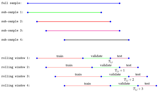
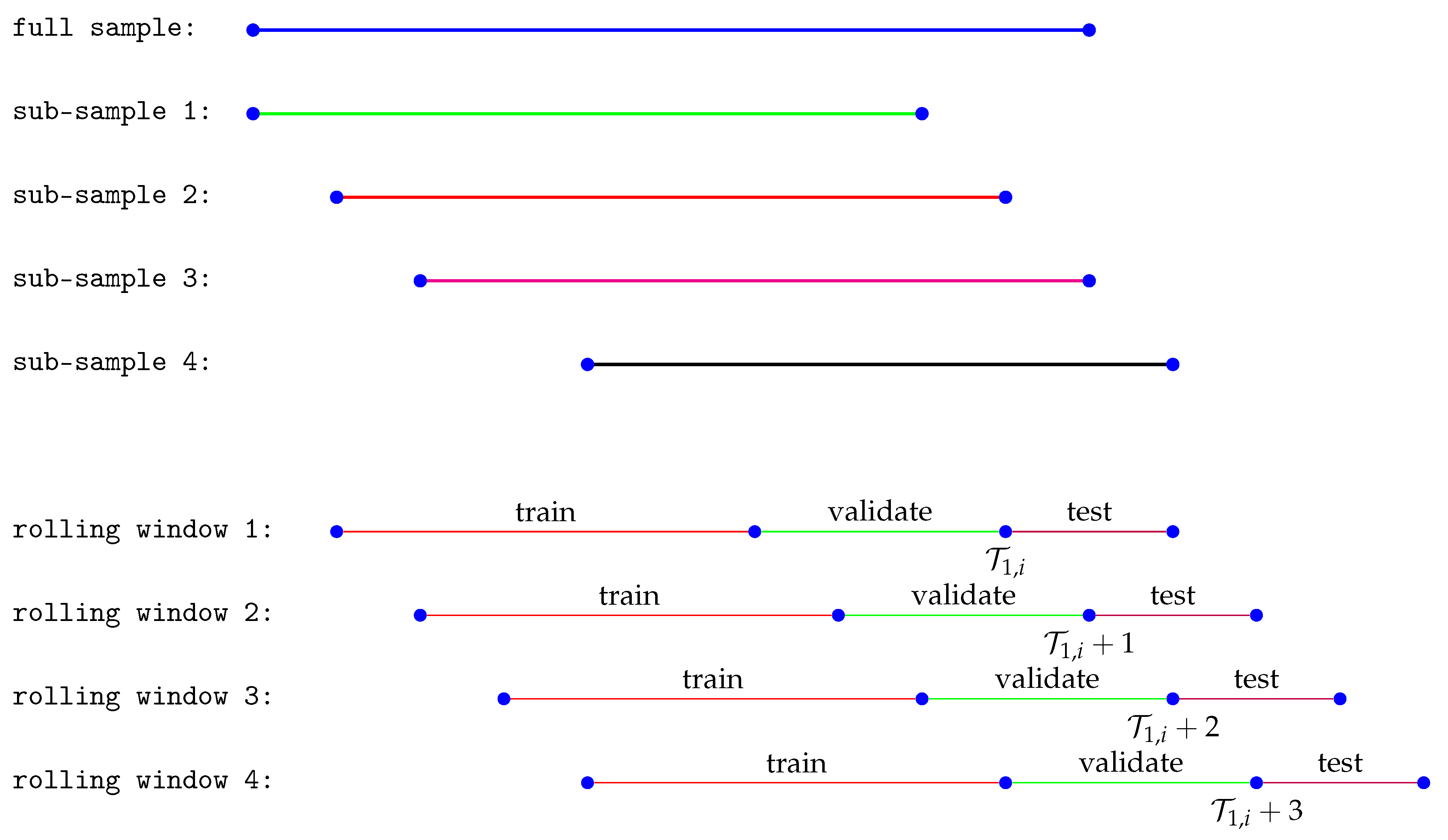
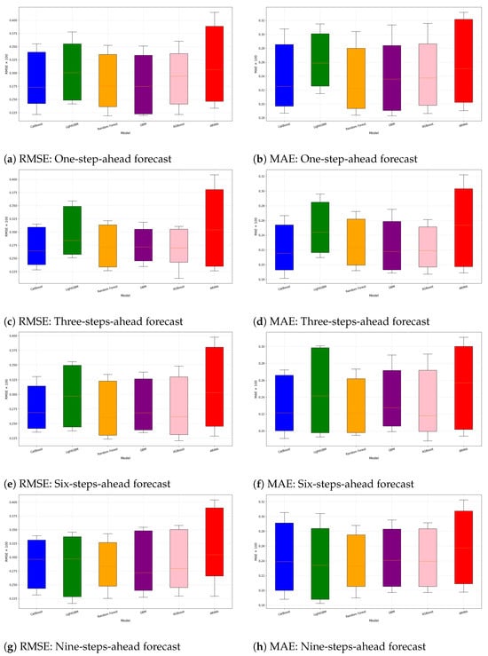
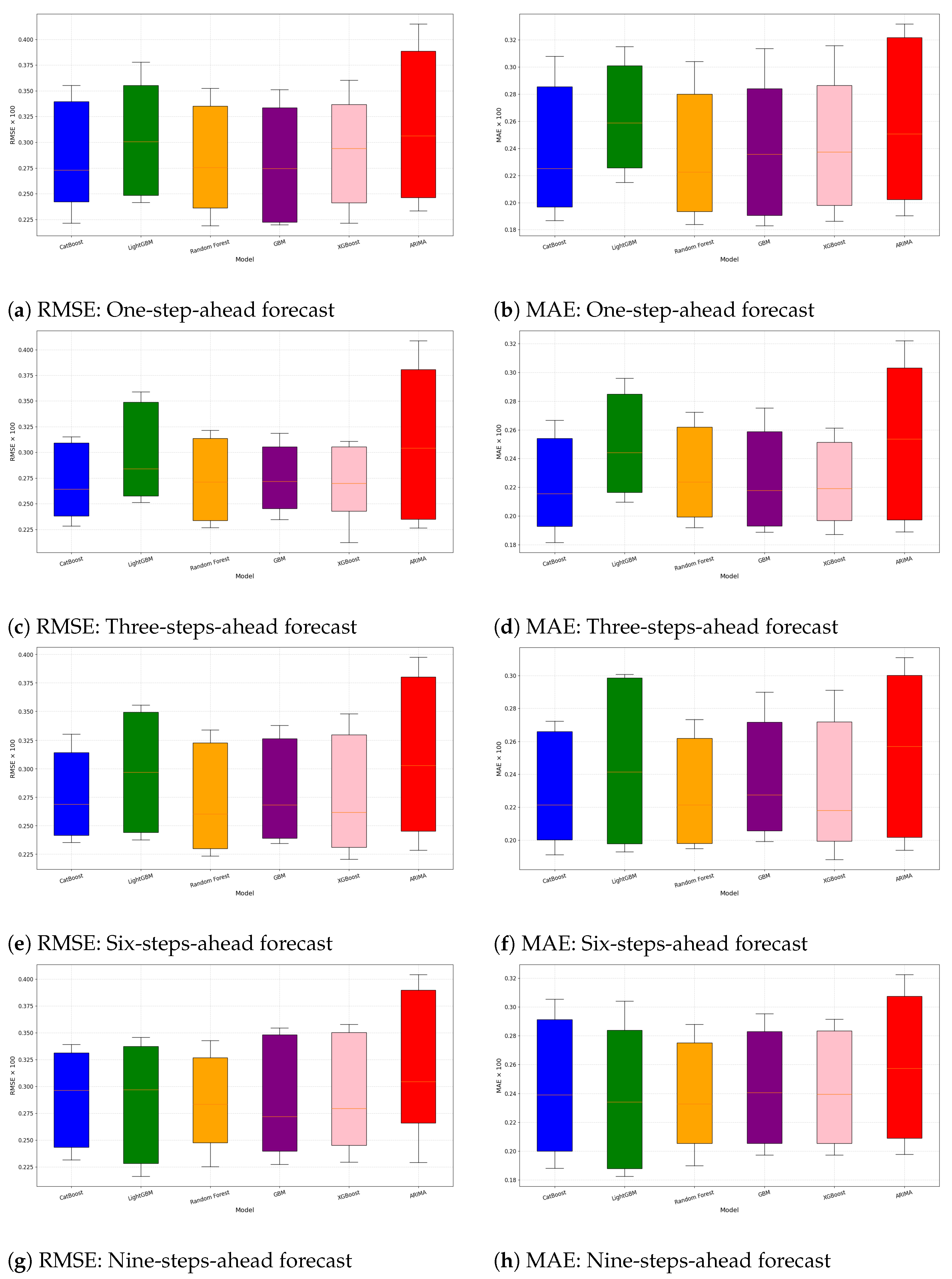
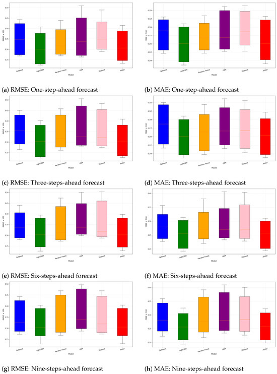
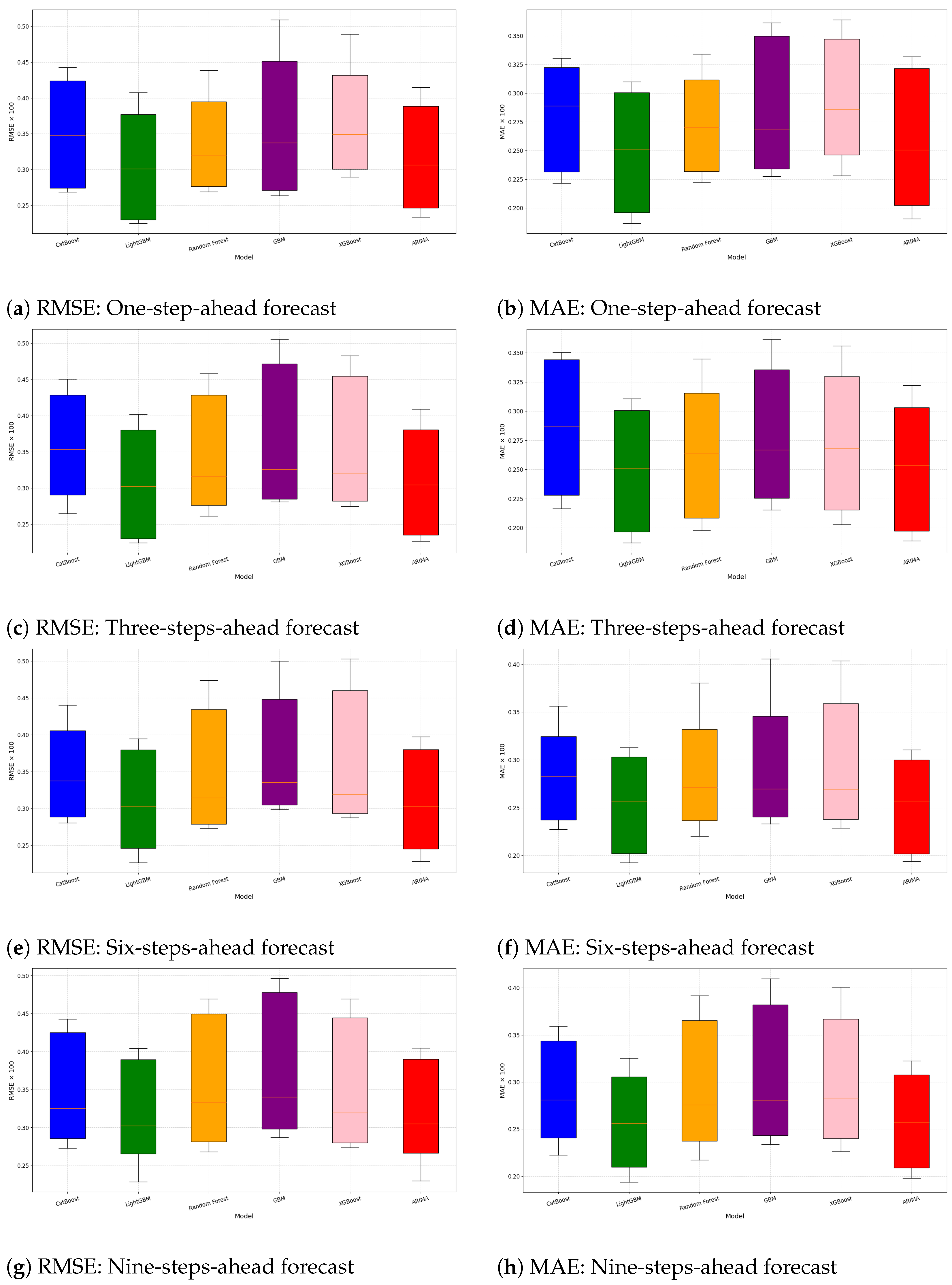
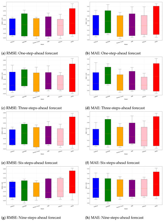
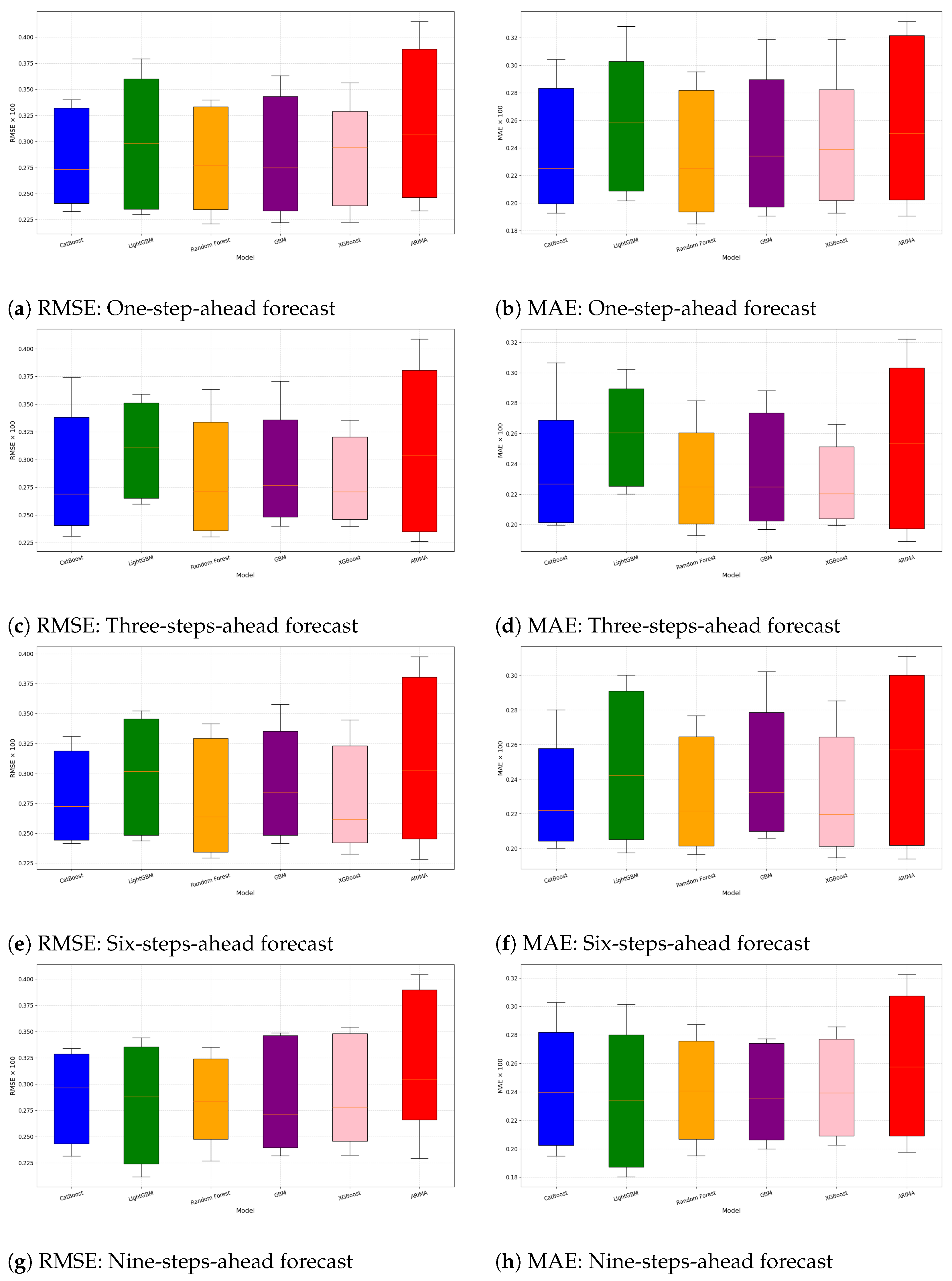

Disclaimer/Publisher’s Note: The statements, opinions and data contained in all publications are solely those of the individual author(s) and contributor(s) and not of MDPI and/or the editor(s). MDPI and/or the editor(s) disclaim responsibility for any injury to people or property resulting from any ideas, methods, instructions or products referred to in the content. |
© 2026 by the authors. Licensee MDPI, Basel, Switzerland. This article is an open access article distributed under the terms and conditions of the Creative Commons Attribution (CC BY) license.