


Abstract
With the advent of the big data era, data becomes increasingly important, especially for many machine learning tasks where data quality is vital. However, missing data is inevitable in many real-world applications, making its handling a challenging problem. Although some reviews exist, they either treat it as a statistical problem or focus only on traditional machine learning methods. This survey provides a novel taxonomy of missing data-handling methods. According to feature or label missing, we classify them into feature-missing handling methods and label-missing handling methods. For feature-missing handling methods, we further categorize them into four classes: traditional, deep learning, soft computing, and large language model missing data-handling methods. Each class is further split to introduce representative methods. For missing-label handling methods, we focus on label completion and distinguish active learning, which selects unavailable labels for acquisition from an oracle, from semi-supervised learning, which estimates unavailable labels from labeled and unlabeled data. For each category, we list their advantages, disadvantages, and applications. To facilitate engineers and researchers, some commonly used software is introduced. To promote further development, we point out challenges requiring deeper investigation.
1. Introduction
High-quality data is the foundation of many machine learning tasks. However, in practical applications, missing data is inevitable due to a variety of factors such as machine failure, human error, no answer to some questions, withdrawal from the study, and multi-source information integration [1,2]. For example, in diabetes prediction research, certain patients can miss Computed Tomography (CT) diagnosis information due to machine malfunction or miss diabetes pedigree information due to unknown or imprecise information. Missing data are ubiquitous in social investigation [3], finance [4], medical informatics [5,6], intelligent traffic [7,8], electronic commerce [9] etc. Missing data has been widely studied in statistical analysis fields [4], especially Little and Rubin [4] systematically investigated data missing mechanisms, data missing patterns, and data missing handling methods with statistical analysis theory. Although the missing data-handling methods have been extensively explored from a statistical perspective, machine learning, especially deep learning and large language models, have achieved remarkable success in many fields recently, providing new opportunities for learning from incomplete and uncertain data [10]. To sort out the existing missing data-handling methods and put them into the AI era, we aim to figure out which part of these methods is going to be progressed further, what limitations or disadvantages the existing methods have, as well as how to overcome them.
Different from a statistical analysis view, we review the existing missing data-handling methods from a machine learning perspective. We categorize them by whether features or labels are missing: feature-missing handling methods and label-missing handling methods. For feature-missing handling methods, we further classify them into traditional methods, deep learning methods, soft computing methods, and large language model methods. For traditional methods, we split them further into instance-level similarity-based methods, feature-level similarity-based methods, Expectation Maximization (EM), and uncertainty-based methods. For deep learning methods, we split them further into Multi-layer Perceptron (MLP)-based methods, Auto-Encoder (AE)-based methods, Graph Neural Network (GNN)-based methods, and Generative Adversarial Network (GAN)-based methods. For large language model methods, we split them further into prompt-based methods and fine-tuning-based methods. Label-missing handling methods are organized into active learning and semi-supervised learning according to whether unavailable labels are acquired from an oracle or estimated from labeled and unlabeled data. The full taxonomy is shown in Figure 1. Furthermore, a comprehensive comparison of these data-handling methods is provided in Table 1, highlighting their characteristics. To facilitate engineers and researchers in dealing with missing data, some commonly used software is introduced.
Figure 1.
The taxonomy of missing data-handling methods.
Table 1.
Taxonomy summary and primary handling roles of missing data methods.
Although the missing data-handling methods have achieved great success, there are still many challenges that hinder their further advancement. We list several challenges and hope that more efforts should be made to advance the development of missing data-handling methods. With this survey, we hope that readers can gain a comprehensive overview of the existing missing data-handling methods and identify directions for further research.
Table 1 distinguishes method families by their primary handling roles. These roles also determine which parts of the evaluation framework in Section 3.4 are applicable: completed values permit direct reconstruction assessment, whereas methods without completed outputs are evaluated primarily through downstream performance, calibration, robustness, and resource use.
Previous reviews have examined missing data from statistical perspectives [11,12,13,14], within pattern classification [15], in longitudinal studies [16], or with an emphasis on traditional feature-missing methods [17,18,19,20]. This survey provides a comprehensive machine-learning-oriented organization of feature- and label-missing handling methods. It groups feature-missing approaches into traditional, deep learning, soft computing, and large language model methods, and examines active and semi-supervised learning within a label-completion perspective. The survey also identifies methodological and evaluation challenges for further study.
The rest of the study is organized as follows. Section 2 describes the literature search and study selection process adopted in this review. Section 3 introduces some related concepts, including data missing mechanisms, common ways to handle missing data, and performance metrics; Section 4 introduces traditional missing data-handling methods; Section 5 introduces deep learning-based missing-data-handling methods; Section 6 introduces soft computing methods to handle missing data; Section 7 introduces large language model-based missing-data-handling methods; Section 8 introduces label completion methods. Section 9 presents some commonly used missing-data-handling software. Section 10 discusses several challenges worthy of further research. Finally, Section 11 presents the conclusions.
2. Review Methodology
The review focuses on feature-missing and missing-label handling, covering traditional, deep learning-based, soft computing, large language model-based, and missing-label approaches within a unified classification framework. The literature search was conducted in Web of Science Core Collection, Scopus, IEEE Xplore, ACM Digital Library, ScienceDirect, and PubMed, with Google Scholar additionally used to identify recent relevant studies. The search combined the keywords “missing data”, “missing value”, “incomplete data”, “data imputation”, “missing label”, “unlabeled data”, “unlabelled data”, “incomplete supervision”, “label scarcity”, “active learning”, and “semi-supervised learning”. The search covered literature published up to 1 August 2026.
Studies were considered relevant if they proposed, extended, analyzed, or applied methods for missing features or missing labels. After duplicate removal, titles and abstracts were screened to exclude irrelevant studies or those lacking a relevant methodological contribution. Within each category, selection considered methodological representativeness, completeness of description, and contribution to the category. Original works and representative extensions were prioritized; among highly similar studies, preference was given to those offering distinct methodological developments, representative applications, or substantive discussions of limitations. This process reduced redundancy while maintaining coverage of the predefined categories. The search yielded 243 records, of which 169 studies were retained for the final synthesis following duplicate removal, relevance screening, and category-based selection.
3. Data Missing Related Concepts
3.1. Data Missing Definition
For a unified treatment of feature and target-label missingness, consider a conceptually complete supervised dataset , where N is the number of samples, is the feature vector, and is the target label. We define feature missingness and target-label unavailability separately on this same complete dataset.
Feature missingness concerns an unavailable component of the input vector. Let and denote the missing and observed feature values, respectively. The feature-missing indicator matrix is defined as
For the feature matrix , if for at least one pair , the dataset has feature missingness; if for all i and j, it is feature-complete.
Target-label unavailability concerns the missingness of , even when its input vector is available. We define the label-missing indicator as
The information available for label completion can be written as the labeled set and the unlabeled input set . A label-completion problem exists when . Its goal is to assign an estimated or newly acquired label to samples for which , using , , and any admissible auxiliary information.
Within this completion-oriented scope, active learning and semi-supervised learning address two complementary questions. Active learning determines which unavailable labels should be acquired from an oracle under a labeling budget, thereby selecting the entries to be completed with verified labels. Semi-supervised learning uses the observed labels and the structure of both and to estimate unavailable labels, for example, through predictive or pseudo-labeling procedures. We therefore organize these methods by their principal role in label completion: label selection and label estimation, respectively.
3.2. Data-Missing Mechanism
The missingness mechanism determines which assumptions connect the missingness pattern to the conceptually complete data and therefore affects identification, estimation, and uncertainty. Let R denote the feature-missing indicators and label-missing indicators introduced in Section 3.1. For a realized complete missingness pattern , let and denote the observed and unobserved components, respectively, of the conceptually complete analysis variables. Following Rubin’s framework [21], MCAR, MAR, and MNAR are defined for each such pattern.
MCAR means that the probability of a missingness pattern is independent of both the observed and unobserved values:
MAR means that, after conditioning on the observed components, the probability of a missingness pattern does not depend on the unobserved components:
MNAR applies when the MAR equality does not hold for at least one pattern and data configuration; after conditioning on the observed components, the missingness probability still depends on at least one unobserved component:
MAR and MNAR are generally not identifiable from the observed data alone [22,23]. The equal observed-data fit of an MNAR model and an MAR counterpart is an observational-equivalence result, not a conversion of the underlying mechanism [23]. An MNAR process may be treated as conditionally MAR relative to an expanded observed information set only when additional variables Z are available and the assumption is scientifically justified. Without this condition, MNAR requires explicit modeling and sensitivity analysis. Label unavailability can arise under MCAR, MAR, or MNAR; its classification depends on the relation between the label-missing pattern, the observed information, and the unobserved labels.
3.3. Common Ways to Tackle Missing Data
Currently, the common ways to tackle missing data are grouped into three classes: no treatment, deletion, and imputation [24,25]. No treatment refers to ignoring the missing value and conducting the task at hand directly. The methods with missing indicator matrix [6,26] are representative methods of this class. This class of methods keeps the original information of the dataset, but they can cause difficulty for modeling. The deletion method constructs a complete dataset by deleting the data points with missing features. Obviously, deletion is simple and easy to use, but it will lose some useful information. Imputation estimates the missing values from the observed values and then fill in. There are many imputation approaches, including single imputation [27,28] and multiple imputation [29,30]. Single imputation includes mean imputation [27,31], regression imputation [28,32], nearest neighbor imputation [5,33], expectation–maximization imputation [34,35], cold deck imputation [31,36], hot deck imputation [31,37] and so on. These types of methods will keep the size of the imputed data and the original data the same; meanwhile, the imputed data is complete, making it easy to conduct tasks by modeling.
3.4. Performance Metrics
Evaluation should be matched to the data type, the output of a missing-data-handling method, and the intended use of that output. The complementary dimensions considered here are pointwise numerical reconstruction; hard-label or probabilistic categorical prediction; distribution and dependency preservation; uncertainty quality; downstream task utility; robustness across missingness settings; and computational or annotation cost. No single metric is sufficient across these dimensions.
Let { is artificially hidden for evaluation and its ground truth is retained} be the evaluation set. Natural missing entries whose true values are unavailable are not members of and cannot be used directly to compute reconstruction error. Numerical pointwise metrics are defined on as follows:
where is the retained ground truth and is the corresponding imputed value.
Smaller MAE, MSE, and RMSE values indicate closer pointwise agreement between imputed numerical values and their ground truth. These metrics are most directly applicable when a method explicitly reconstructs missing values, including two-stage impute-then-analyze pipelines, and when ground truth can be withheld for evaluation.
For hard categorical outputs, completion accuracy and macro-F1 measure exact recovery and class-balanced performance, respectively. For m held-out categorical entries with C possible classes, probabilistic predictions can be evaluated using the Brier score:
where is the predicted probability that the ith missing entry belongs to class c, and is one if the observed ground-truth class is c and zero otherwise. A smaller Brier score indicates better probabilistic categorical prediction. Because the score jointly reflects calibration and discrimination, it should be complemented by calibration diagnostics when reliable probabilities are an explicit objective.
Pointwise agreement does not ensure preservation of the data distribution. Let P denote the empirical distribution of the ground-truth values and the distribution after imputation. Their p-Wasserstein distance is
where is the set of couplings with marginals P and . A smaller value indicates closer distributions. Wasserstein distance alone does not establish that the dependencies required by an analysis have been preserved. Depending on the scientific objective, evaluation should therefore also compare marginal distributions, covariance or correlation structure, task-specific cross-variable dependencies, and relevant tail behavior. For probabilistic or multiple-imputation methods, uncertainty should be evaluated through calibration or interval coverage together with interval width, since narrow but poorly calibrated intervals can be misleading.
Robustness should be tested on common data splits and missingness masks across multiple missing rates and scientifically plausible MCAR, MAR, or MNAR settings. Repeated runs should report variability rather than only the best result. Resource reporting should include the quantities relevant to deployment, such as training and inference time, peak memory, model or API access, and, for active label acquisition, annotation cost and performance as a function of the labeling budget.
Downstream-task performance is essential for both explicit imputation and methods that operate directly on incomplete data. Examples include accuracy, macro-F1, area under the receiver operating characteristic curve, and calibration for classification; predictive error for regression; adjusted Rand index or normalized mutual information for clustering; and task-specific ranking metrics for recommendation. For explicit imputation methods, reconstruction, distribution, and dependency measures should be reported together with downstream results because good reconstruction does not guarantee task utility. For methods that do not generate a completed dataset, entry-wise imputation metrics are generally unavailable, so held-out downstream performance, calibration when applicable, robustness, and resource use should serve as the primary evidence. This output-aware protocol is used to interpret the method comparisons throughout this survey and is discussed further in Section 10.5.
4. Traditional Methods
4.1. Instance-Level Similarity-Based Methods
Instance-level similarity-based methods aim to look for some similar data points to the incomplete data point and then fill in the missing feature values of the incomplete data point by referring to the observed feature values. To achieve this goal, several methods have been proposed. They are mean imputation, K-nearest neighbors imputation, hot-deck imputation, cold-deck imputation, and clustering-based imputation.
Mean or mode imputation is a simple deterministic baseline. For a numerical feature, missing entries are replaced by an estimated mean from the eligible observed training values; for a categorical feature, the mode is commonly used. The fitted statistic must be computed without using held-out test information. Although computationally inexpensive, this procedure reduces within-feature variability and can distort marginal distributions, associations, standard errors, and downstream analyses. Mohamed et al. [38] studied variants intended to account for aspects of the feature distribution.
K-nearest-neighbor imputation identifies K complete nearest neighbors of each incomplete data point and then weights these K complete nearest neighbors to obtain the imputed values at missing positions in incomplete data points. This method consists of two stages: identifying K-nearest neighbors and calculating the weights corresponding to the nearest neighbors. During the K-nearest neighbors identification stage, different distance formulations can be adopted [39], such as Euclidean distance, Minkowski distance, Mahalanobis distance, and cosine distance. When calculating the weights corresponding to these nearest neighbors, many strategies can be adopted. For example, calculate the distance between the incomplete data point and its K-nearest neighbors and use the reciprocal value of those distances as the weights; thus, near neighbors will contribute more than distant neighbors. Since the selection of distance and K will affect the imputation results, several evolutionary K-nearest neighbor imputation approaches are designed to boost the imputation performance by optimizing the selection of distance and K [40].
Hot-deck imputation fills a missing entry using values from one or more observed donor records in the current donor pool. Nearest-neighbor matching is one possible donor-selection rule, while random selection within adjustment cells and fractional weighting provide other designs [41,42]. Its behavior depends on how the donor pool, matching variables, distances, and weights are defined. Cold-deck imputation instead obtains donor values from an external or historical source [36], so its validity also depends on the comparability of that source with the target data.
Clustering-based imputation uses estimated subgroup structure to select prototypes or donor records for missing entries [43,44]. Standard clustering algorithms that require complete vectors need an initial completion, whereas incomplete-data clustering methods can modify distances or jointly update cluster assignments and missing values. Some procedures alternate clustering and imputation until a declared stopping condition is met [45]. Scalability and imputation quality depend on the clustering algorithm, initialization, distance under missingness, cluster validity, number of clusters, data size, and stopping rule; large sample size alone does not establish superiority over other methods.
4.2. Feature-Level Similarity-Based Methods
Feature-level similarity-based methods impute the missing values by regression modeling to mine the correlation of data features. They mainly include linear regression-based methods and nonlinear regression-based methods. Linear regression-based methods impute the missing values by modeling features linearly, while nonlinear regression methods impute the missing values by modeling features nonlinearly.
For target-wise regression imputation of feature k, let and let denote the predictor subvector. A complete-predictor training set is
On this set, a linear conditional model can be written as
where and is a residual term. The least-squares objective is
After fitting on , the model can predict for records with when the required predictors are available. If some predictors are also missing, the procedure must specify a complete-predictor subset, an initial imputation, a missingness-aware model, or a chained-equations strategy. Feature selection or regularization may be used when only part of is informative [46].
A nonlinear conditional model replaces the linear predictor with a specified function:
with objective
For illustration, when f uses a single observed predictor , common parametric forms include
- Polynomial functions ;
- Exponential functions ;
- Logarithmic functions , defined for ; and
- Power functions on an appropriate domain.
Neural networks and compositions of basis functions provide more flexible choices for f. When several target features are incomplete, separate conditional models may be fitted and iterated, as in sequential regression or chained-equations procedures [47]; the order, predictor availability, and initialization must then be stated.
4.3. Expectation Maximization
The general EM framework was formalized by Dempster, Laird, and Rubin [48] in 1977; further theory and applications are described by McLachlan and Krishnan [49]. EM estimates parameters in models with latent or missing data. Let and denote the observed and missing components and let be the current parameter estimate. The E-step forms the expected complete-data log-likelihood
and the M-step updates the parameters by
Under standard regularity conditions, these updates make the observed-data likelihood non-decreasing. They do not generally guarantee a global optimum: the final stationary point and convergence rate can depend on the probabilistic model, parameterization, implementation, and initialization. An EM-fitted model may subsequently provide conditional expectations or draws for missing values, but parameter estimation and the choice of a completed-data summary are distinct steps.
Several cited studies evaluated EM-based procedures in specific settings. García-Laencina et al. [50] applied EM imputation to breast-cancer survival prediction with incomplete discrete variables. Musil et al. [51] reported favorable results for EM relative to the deletion, mean-imputation, and regression variants included in their experiments, while Nelwamondo et al. [34] compared EM with a genetic-algorithm and auto-associative-neural-network procedure. These findings are conditional on the datasets, missingness settings, comparators, and metrics used in the respective studies; they do not establish uniform superiority of EM.
4.4. Uncertainty-Based Methods
Multiple imputation (MI) represents missing-data uncertainty through several completed datasets rather than a single deterministic completion [29,52]. A proper MI procedure generates completed datasets using draws from an appropriate posterior-predictive or repeated-sampling distribution conditional on the observed data. Each completed dataset is analyzed separately, and the estimates are combined using Rubin’s rules so that within-imputation and between-imputation variation contribute to the reported uncertainty. The general workflow is illustrated in Figure 2.
Figure 2.
The whole process of MI to deal with incomplete data.
Merely rerunning a deterministic single-imputation rule does not constitute proper MI. The procedure must propagate uncertainty in missing values and, where required for valid inference, uncertainty in estimated model parameters. Implementations include Bayesian procedures, resampling-based procedures, and chained-equations methods with suitable stochastic draws [53,54,55,56]. MI is intended to improve uncertainty propagation for subsequent analysis; it does not guarantee lower pointwise reconstruction error for every dataset, missingness mechanism, or metric.
Each of these traditional learning methods has its own advantages, disadvantages, and application scenarios, as demonstrated in Table 2.
Table 2.
Comparison of traditional machine learning methods for missing data.
5. Deep Learning Methods
In the past two decades, deep learning has obtained tremendous success in many areas. Several deep learning models have been modified to cope with the missing data problem. According to the basic model adopted, deep learning methods to tackle the missing data problem can be classified into four groups: MLP-based methods, AE-based methods, GAN-based methods, and GNN-based methods.
5.1. MLP Based Methods
MLP-based imputation can model nonlinear conditional relationships between a target feature and the available predictors [57,58]. For a target-specific MLP that imputes feature k, let be the predictor vector defined in the regression subsection. A network with two hidden layers and one scalar output can be written as
Here, , , , and the bias vectors have the corresponding hidden-layer dimensions. The functions , , and are the chosen activations. Figure 3 illustrates this target-specific workflow.
Figure 3.
The MLP model to deal with missing values.
The network in Equation (18) is trained only on records for which the target and the predictors required by the network are available, such as . It is then applied to records with . When predictor features are also missing, the method must specify an initial completion, a mask-aware architecture, or another joint strategy; this choice can materially affect the result. A target-specific MLP is one nonlinear-regression design, while multi-output and joint architectures can impute several features simultaneously [59].
5.2. AE-Based Methods
An autoencoder (AE) learns a representation by reconstructing its input. With encoder parameters and decoder parameters , a basic AE is
The reconstruction loss and the treatment of unavailable inputs must be specified by the imputation method. Common designs provide an initial fill together with a mask, corrupt observed entries during training, or compute a loss only where a target value is known. Figure 4 depicts the basic encoder–decoder structure.
Figure 4.
The AE model.
Denoising AEs learn to reconstruct clean targets from corrupted inputs [60]. Corruption may use masking, Gaussian noise, or another declared process [61]; it should not be conflated with naturally missing entries whose ground truth is unavailable. A variational autoencoder (VAE) instead introduces a latent variable and maximizes the evidence lower bound [62]:
For incomplete-data VAEs, the encoder conditioning and likelihood term must be adapted to the observed components and, where used, the missingness mask. Adversarial autoencoders [63] use an adversarial regularizer to match the aggregated latent distribution to a chosen prior. This mechanism is not the same variational objective as the VAE ELBO.
A tracking-removed AE is proposed in Ref. [64] to fill in the missing values. In this work, the connection from the output neuron to its corresponding input neuron is removed to weaken the self-trackability of the network to avoid learning the identification function. A multitask learning method where DAE imputes the missing values and a classification task is conducted simultaneously is provided in Ref. [65]. Similar works are proposed in Refs. [66,67]. Ref. [65] provided a modified VAE to tackle the heterogeneous data-missing problem with different likelihood models for different data types. An adaptive-learned median-filled deep auto-encoder (AM-DAE) is proposed to tackle the industrial time-series data missing problem [68,69,70].
5.3. GAN-Based Methods
GAN is a machine learning framework with two neural networks competing with each other, inspired by game theory [71]. The GAN framework is illustrated in Figure 5.
Figure 5.
GAN framework.
In the standard GAN framework shown in Figure 5, the generator maps noise to generated samples, and the discriminator distinguishes observations from generated samples. The minimax objective is
For this objective, D is trained to increase for observed samples and for generated samples, while G is trained adversarially. Practical implementations often use the non-saturating generator loss instead of directly minimizing the second term.
Equation (21) is a background objective rather than a complete specification of an imputation model. VIGAN combines adversarial view-to-view mapping with a multimodal denoising AE [72]; GAIN uses a mask and hint mechanism so that its discriminator identifies which components were observed [73]; and MisGAN explicitly models the missingness mask [74]. Other variants have been evaluated for high missing rates, time-series data, medical images, and traffic data [75,76,77,78,79]. Their objectives, assumptions about missingness, and evaluation settings differ, so the standard GAN objective alone does not imply calibrated or accurate imputations.
5.4. GNN-Based Methods
GNNs provide a way to model relational structure among samples, features, or both when handling incomplete data. Graph completion [80,81] and link prediction [82] supply related formulations. GRAPE represents an incomplete table as a bipartite graph whose sample–feature edges carry observed values, and formulates imputation as edge-level prediction [83]. Its framework is shown in Figure 6.
Figure 6.
Graph framework Grape to handle missing values, where “?” indicates missing values.
In Figure 6, indicates the ith sample and indicates the jth feature, represents the value that the ith sample takes on the jth feature. For instance, . The nodes on one side of the bipartite graph are represented as , and the nodes on the other side are represented as ; the connections between the nodes on both sides are represented as . indicates the jth feature value of the ith sample. If the connection is unknown, it means that the corresponding feature of the corresponding sample is missing.
Grape treats all samples equally due to the lack of relational information between samples. To address this issue, Ref. [84] proposed an improved imputation approach with iterative graph reconstruction to exploit the relationship between samples. Ref. [85] proposed an inductive matrix completion approach by utilizing Graph AE to learn the local graph patterns so as to generalize to unseen data. Ref. [86] designed an augmented neural network to learn the relationship between the node and attribute to achieve attribute completion. Ref. [87] proposed a two-stage imputation method composed of initialization and refinement, which is a graph attribute imputation network. Attribute and structure information are used interactively to impute missing graph attributes in Siamese attribute-missing GAE [88]. Ref. [89] proposed a Wasserstein Graph Neural Network to exploit the observed attribute information to achieve the attribute completion goal. Each of these deep learning methods has its own advantages, disadvantages, and application scenarios, as shown in Table 3.
Table 3.
The comprehensive comparison of deep learning missing data-handling approaches.
6. Soft Computing Methods
Soft computing [92] aims to design approximate models to solve complex real-world problems. Different from traditional computing techniques, soft computing is tolerant of uncertainty, inaccuracy, noise, and approximations; thus, it is suitable for tackling missing data problems. According to the different soft computing techniques adopted, soft computing approaches are classified into fuzzy set-based methods and rough set-based methods.
6.1. Fuzzy Sets-Based Methods
As the fuzzy extension of classical sets, fuzzy sets are defined as sets that have different grades of membership [93]. Since the fuzzy set is the foundation, we introduce it firstly.
A fuzzy set A on a universe is characterized by a membership function . For each object , the value is its membership grade in A.
One common way to cope with missing data is to conduct fuzzy clustering for incomplete data and then impute the missing part based on the fuzzy clustering results. For a complete data matrix , fuzzy C-means (FCM) partitions the samples into K clusters by solving [94]
Here, is the membership of sample i in cluster k, is the partition matrix, contains the cluster prototypes, and z is the fuzzifier. Standard FCM requires complete vectors for the Euclidean distances in Equation (22). Incomplete-data variants must instead declare an initial imputation, compute distances on available components with an appropriate correction, or jointly optimize the missing entries with memberships and prototypes.
Based on the partition matrix and prototype matrix, there are three ways to impute missing values: membership weighting imputation, nearest prototype imputation, and feature voting imputation. For the membership weighting imputation method, calculate the membership function for the object with missing values and then use them to weight each prototype to obtain the imputed values [95]. For the nearest prototype imputation method, the complete objects in the same cluster are considered as nearest neighbors, and their values are employed to complete the missing positions of incomplete objects in the same cluster [96]. For feature voting imputation, the cluster each object belongs to is identified by voting from the cluster prediction from each feature, and then the feature value of the nearest neighbor within the identified cluster is used to fill in [97]. Ref. [98] proposed three strategies for FCM to tackle missing data. The whole data strategy just uses the complete data; the partial distance strategy adopts a similar idea with an indicator matrix; the optimal completion strategy treats missing values as variables and learns them with FCM parameters in a whole optimization process. Ref. [96] proposed two fuzzy membership functions to impute time series missing values.
6.2. Rough Sets-Based Methods
Rough sets are an effective technique to analyze and handle inaccurate, inconsistent, incomplete information [99]. Since the majority of information systems are incomplete, rough sets have been extensively used in information systems.
In general, an information system can be represented by , where indicates a finite set of objects and indicates a finite set of attributes. The decision table consists of that indicates the value taken by each attribute of each object . Note that one of the attributes is the decision, while the others are the normal attributes.
For an attribute subset , the P-indiscernibility relation is . Its equivalence classes form the partition , also denoted . If , the objects x and y cannot be distinguished using the attributes in P.
Given an object subset and an attribute subset , let denote the equivalence class of x under . The P-lower and P-upper approximations are
The rough representation of X is the pair . The lower approximation contains objects whose equivalence classes are wholly contained in X, whereas the upper approximation contains objects whose equivalence classes have a nonempty intersection with X.
In reality, there are many missing values in decision tables. They can be grouped into three types: lost values, attribute-concept values, and “do not care” conditions [100]. Lost values mean that these values were kept but are not available presently; attribute–concept values indicate that the values can be filled in with the value of the corresponding attribute of any objects in the same concept (equivalence class); “do not care” conditions indicate irrelevant missing values. For the lost values case, two modified rule induction methods, LEM1 and LEM2, are proposed [101]. A non-symmetric similarity relation and a valued tolerance relation to handle the lost values are proposed in Ref. [102]. For attribute–concept values, an attribute–value pair block is proposed to deal with this incomplete case [103]. For “do not care” conditions, Ref. [104] proposed a rule induction method to convert an incomplete decision table to a complete decision table. In general, the characteristic relations, instead of the indiscernibility relations, are adopted to describe the incomplete decision tables [105].
Table 4 summarizes the mechanisms, limitations, and reported application areas of the reviewed fuzzy-set and rough-set methods. These entries characterize the cited designs and should not be interpreted as a performance ranking against newer method families.
Table 4.
The comparison of soft computing missing data-handling approaches.
7. Large Language Model Methods
Large language models are generally categorized into three major architectural types: encoder-only, decoder-only, and encoder–decoder models. Representative encoder-only models such as BERT [106] and RoBERTa [107] are primarily designed for understanding-oriented tasks, including text classification and semantic matching. Decoder-only models, including LLaMA [108], are commonly used for generation-oriented tasks such as text completion, dialog, and open-ended question answering. Meanwhile, encoder–decoder architectures like T5 [109] combine an encoder and a decoder for sequence-to-sequence prediction. For data imputation, the architecture should be selected according to whether the workflow emphasizes representation learning, conditional generation, or sequence-to-sequence transformation. The reviewed evidence does not support assigning general prevalence or superiority to one architecture. The final output distribution of a decoder-only model for the next token is typically computed via a softmax transformation:
where is the hidden representation at time step t and is the output projection matrix. Through this probabilistic generative formulation, LLMs can infer or reconstruct missing components by leveraging learned contextual dependencies. In practice, LLM-based data imputation methods can be broadly categorized into two types: prompt-based and fine-tuning-based methods.
7.1. Prompt-Based Methods
Prompt-based methods exploit the zero-shot learning ability of LLMs to impute missing data through designed prompts. As shown in Figure 7, the key idea is to reformulate data imputation as a text completion task, where each data record is serialized into a textual sequence, and the model predicts plausible values for missing fields based on contextual cues. Formats such as markdown or natural language are commonly used due to their compatibility with the textual pretraining of LLMs [110].
Figure 7.
Prompt-based method to handle missing values.
Retrieval-Augmented Generation (RAG) introduces external information retrieval into the imputation process to supplement the model’s limited context and static parametric knowledge [111]. Retrieved records can provide additional context, but their contribution depends on retrieval relevance, source quality, and the model’s use of the retrieved evidence. Retrieval alone does not ensure accurate or reliable imputation. Recent work includes both table-level and fine-grained tuple-level retrieval, where frameworks such as Retrieval-Augmented Imputation (RAI) use specialized encoders to identify semantically aligned records [112]. Iterative refinement and self-consistency mechanisms have also been studied as ways to reduce output variability rather than as guarantees of robustness. Self-refinement enables LLMs to function simultaneously as generators and critics, iteratively revising their outputs through feedback loops [113]. Self-correction strategies extend this principle by integrating external evaluators or downstream feedback signals, exemplified by the IMPROVE framework [114]. In parallel, self-consistency sampling aggregates multiple reasoning trajectories and selects a consensus outcome to reduce sensitivity to a single stochastic generation [115].
7.2. Fine-Tuning-Based Methods
Fine-tuning-based methods adapt pretrained models or attached modules to an imputation domain. Their objectives are architecture- and representation-dependent: encoder-only models may use masked-token prediction, decoder-only models generally use causal or conditional language modeling, encoder–decoder models may use sequence-to-sequence reconstruction, and hybrid imputers may add numerical reconstruction or downstream-task losses. As a generic notation, let be the target set of masked or unavailable entries used during supervised training, and let contain any schema, prompt, or auxiliary context. An entry-level conditional objective can be written as
where may be a token probability, a categorical probability, or a continuous density chosen for the represented value. Equation (25) is only a unifying conditional notation; it does not imply common tokenization, architecture, or loss across all LLM-assisted imputers.
In base fine-tuning, some or all pretrained parameters, or parameter-efficient adapters such as Low-Rank Adaptation (LoRA) [116], are updated for the target domain. Applied settings include biomedical or clinical records [117], missing table entries, and pseudo-sample generation [118]. These systems are not necessarily end-to-end in the same sense: preprocessing, serialization, retrieval, constrained decoding, and downstream modules may remain separate. Their utility depends on representation choices, training data, model access, the treatment of numerical values, baselines, and the evaluation protocol.
Hybrid architectures combine a pretrained language model with encoders, graph modules, time-series components, retrieval systems, or task-specific completers [119]. The language model may supply semantic representations or contextual information without directly producing the final numerical or structured imputation. The reviewed systems can be organized into two common designs. The first approach focuses on transforming heterogeneous information into formats comprehensible by LLMs. Structured or semi-structured data, such as knowledge graphs, tabular data, or spatiotemporal sequences, are encoded into natural language descriptions or other serializable representations that LLMs can process for reasoning and imputation. Representative methods include CRILM, which generates contextually relevant textual descriptions to complete missing values in knowledge graphs [120] and ImputeFormer, which encodes spatiotemporal data using a low-rank Transformer and leverages LLMs for completion [121]. The second approach emphasizes first extracting useful information from the data using LLMs, and then employing specialized completer modules for imputation. In this framework, LLMs generate multi-perspective descriptions or contextual embeddings to represent entity relationships, structural patterns, or latent features, which are subsequently used by dedicated imputation mechanisms. For example, LREC queries LLMs from multiple perspectives to expand entity representations and extract relational structures for knowledge graph completion [122], while GATGPT integrates graph attention networks with LLM-generated contextual information to impute spatiotemporal data [123].
Table 5 summarizes the capabilities, limitations, and application settings of prompt-based and fine-tuning-based LLM methods. LLM-assisted imputation is an emerging branch of missing-data research for semantically rich tables, text fields, knowledge graphs, and workflows that use external knowledge. Evidence across these settings remains heterogeneous, and controlled comparisons with statistical, deep generative, graph-based, diffusion, and tabular foundation models remain limited. Its applicability depends on the data representation, available semantic information, computational resources, privacy requirements, and model access.
Table 5.
The comparison of large language model missing data-handling approaches.
8. Label-Missing Handling Methods
Following the definition in Section 3.1, label completion includes active learning for selective oracle annotation and semi-supervised learning for estimating unavailable labels from labeled and unlabeled data. A practical workflow may combine the two components.
8.1. Active Learning
In a label-completion workflow, active learning determines which samples with unavailable labels should be sent to an oracle (e.g., a human annotator), which then supplies the verified labels. Under a finite annotation budget, query strategies can be broadly grouped into uncertainty-based and representation-based methods.
An uncertainty-based method selects the sample with high uncertainty to query. Maximum entropy [125] is commonly used to select the sample with maximum predictive entropy. A sample with the least confidence [126] between the two most likely labels is generally selected for querying. The sample with the smallest margin [127] between two classes is also chosen to query. Feature mixing [128] selects the unlabeled sample with sufficiently distinct features by seeking inconsistencies in predictions resulting from interventions on their representations.
Representation-based methods attempt to select a representative sample of the unlabeled sample set. These types of methods are based on the intuition that once the representative sample is selected to label, it can act as a surrogate for the whole dataset [129]. Pre-clustering [130] proposed a framework to introduce the clustering method into active learning. It trains a classifier with the set of cluster representatives, and then propagates the classification decision to the other samples via a local noise model. Cluster-margin [131] runs hierarchical agglomerative clustering with average-linkage and then chooses a diverse set of samples with the lowest margin scores. Coreset [132] chooses a batch of representative samples based on a core set that is a subset of a dataset that can be seen as a proxy of the full set.
Uncertainty-based strategies prioritize samples on which the current model is uncertain, whereas representation-based strategies aim to cover the unlabeled data distribution. Hybrid strategies combine these criteria either in a weighted objective or in separate representation and selection stages. WAAL [133] learns a discriminative representation before batch selection, while BADGE [129] constructs gradient embeddings and applies KMeans++ to select a diverse batch. Their relative utility depends on the model, batch budget, data distribution, and evaluation protocol.
Active learning addresses which unavailable labels should be completed with oracle-provided values. Its applicability therefore depends on access to an oracle, and annotation latency or cost may make it impractical in real-time scenarios such as autonomous driving.
8.2. Semi-Supervised Learning
Semi-supervised learning (SSL) learns from both labeled and unlabeled data [134]. In the label-completion setting defined in Section 3.1, SSL uses and jointly to learn a predictive function and assigns to samples with . The validity of these completed labels depends on assumptions such as smoothness, cluster structure, low-density separation, or view sufficiency. These approaches can be grouped into three classes: self-training, co-training, and graph-based methods.
Self-training trains a classifier on a small number of labeled data and uses the trained classifier to predict the labels of those unlabeled data, then moves several most confident unlabeled data with their corresponding predicted labels into the training set, and the classifier will be re-trained. This process will be repeated until a certain condition is met. It should be noted that the classifier teaches itself with its own predictions; thus, this method is also known as self-teaching. Generative mixture models [135] and EM [136] can be considered as soft self-training algorithms. Ref. [137] integrated self-training and active learning for video segmentation. Ref. [138] proposed a semi-supervised multi-task method by combining self-training and a probability generalization of SVM. Ref. [139] adopted self-training for machine fault diagnosis.
Co-training [140] is a semi-supervised framework for data represented by two views. Its classical analysis assumes that each view is sufficient for prediction and that the views satisfy an appropriate conditional-independence assumption. Separate classifiers iteratively assign selected predictions from one view to the training data of the other. In the experimental settings studied by Nigam and Ghani [141], co-training was compared with EM [136] and generative-mixture approaches [135]; the reported differences are conditional on those datasets, assumptions, and implementations and do not establish universal superiority.
A graph-based semi-supervised approach defines a graph where the nodes indicate the labeled and unlabeled data points and edges indicate the similarity of these data points. Label smoothness is a common assumption for graph-based semi-supervised approaches. Graph regularization [142] is a classical tool to implement semi-supervised learning [143].
Besides these three groups of semi-supervised learning methods, there are some other methods. Ref. [144] designed a semi-supervised SVM for semi-supervised learning. Ref. [145] proposed a semi-supervised learning method using Gaussian processes. Ref. [146] conducted semi-supervised learning with trees. Ref. [147] provided a semi-supervised learning method via entropy minimization. Ref. [148] introduced sparsity into semi-supervised learning using Fenchel–Legendre conjugates. Ref. [149] proposed to conduct imputation and classification simultaneously in a semi-supervised way.
Table 6 summarizes the roles, limitations, and applications of the two label-completion components.
Table 6.
The comparison of label-missing handling approaches.
9. Software
Researchers from many areas, including statistical learning and machine learning, have developed several tools to handle the missing value problem. To facilitate researchers’ and engineers’ use of them conveniently, some commonly used software is introduced.
PROC MI in SAS 9.4 [151] carries out multiple imputation analysis with three steps. Firstly, use the PROC MI statement to conduct imputation. Secondly, use SAS complete data analysis procedures to analyze the complete dataset obtained from the first step. Thirdly, use the PROC MIANALYZE statement to combine the analysis results.
ICE in Stata 18 [152] mainly handles categorical missing case by imputation with chained equations [153]. Logistic regression is adopted to predict binary missing variables, while an ordered logistic regression or multinomial regression is used to deal with the categorical variables with multiple levels.
Software or packages in R 4.5.3:
- MICE (Multivariate Imputation via Chained Equations) (https://amices.org/mice/, (accessed on 1 July 2026)) is a popular package to conduct imputation for R language users. MICE assumes that the missing data are MAR. It imputes the missing data for each variable by specifying a specific method. The imputation will be conducted by the mice() function, while the results on the imputed data are summarized with the pool() function. The parameter in mice() will identify the specific imputation model for each variable of the input. The generated random INDS dataset will be used in the analysis.
- mi (https://CRAN.R-project.org/package=mi, (accessed on 1 July 2026)) is a popular imputation package in the R language. It can be used to impute data in an approximate Bayesian framework, diagnose the imputation models, validate the imputation algorithm assumptions, and analyze the multiple imputed datasets with the appropriate sampling uncertainty degree.
- missForest (https://CRAN.R-project.org/package=missForest, (accessed on 1 July 2026)) is used for imputing missing cases, particularly mixed-type data, including continuous and/or categorical variables. Based on the observed values, a random forest will be trained to predict the missing values. It is noted that this package can work in parallel; thus, it is computationally efficient.
- Amelia (https://CRAN.R-project.org/package=Amelia, (accessed on 1 July 2026)) is proposed by Ref. [154]. It mainly works for the missing value problem in a time series dataset. It can generate imputations and diagnose the fitting of the MI models. This package is easy to use with either the R command line or graphical user interface.
- Hmisc (https://CRAN.R-project.org/package=Hmisc, (accessed on 1 July 2026)) includes some functions for data processing, data analysis, graphic demonstration, high-class table making, and missing value imputation, feature clustering, character sequence operation, and conversion of R language objects to HTML or LaTeX code.
Grape (https://github.com/maxiaoba/GRAPE, (accessed on 1 July 2026)) is a representative graph representation learning approach to tackle the missing value problem [83]. Within this graph framework, two types of nodes indicate the samples and the features, respectively. The edges between these two types of nodes represent the feature value taken by that sample; the missing value imputation problem is transformed into an edge prediction problem, and label prediction is transformed into a node prediction problem within the bipartite graph.
10. Challenges
10.1. Task-Oriented Case
In practical applications, missing value imputation is rarely the final objective, but usually serves downstream tasks such as classification [155], clustering [156], recommendation [157], risk prediction, and scientific analysis. However, many existing methods still optimize imputation as a standalone reconstruction problem. This creates a gap between numerical recovery and task utility: imputed values with low reconstruction error may not preserve the information most relevant to decision boundaries, clustering structures, ranking quality, or risk estimation. Therefore, future research should move toward task-aware missing data handling, where imputation and downstream objectives are jointly considered. Multitask learning offers a natural framework for this purpose [65,158], while end-to-end missingness-aware models, task-guided imputation objectives, and uncertainty propagation from imputation to prediction are also promising directions. Evaluation should accordingly go beyond imputation error and include downstream performance, robustness, calibration, and sensitivity to imputation uncertainty.
10.2. Restricted Data Access
Missing data handling becomes more challenging when data cannot be directly accessed or centralized. In domains such as healthcare, finance, and enterprise management, data are often distributed across institutions and constrained by privacy, ownership, and regulatory requirements. Although federated imputation has begun to address this problem in heterogeneous electronic health records [159], this direction remains underexplored. The main difficulty is that imputation depends on statistical information such as marginal distributions, cross-variable dependencies, temporal correlations, and missingness mechanisms, which may be fragmented across different sites. Local models may therefore suffer from biased distributional estimates, while centralized training is often infeasible. Future work should study imputation under limited cross-institution information exchange, rather than assuming that distributed training can fully reproduce centralized performance. Important issues include heterogeneous variable spaces, site-specific missingness mechanisms, communication costs, cross-institution generalization, and downstream utility under privacy constraints.
10.3. Missingness Mechanism Identification
Another fundamental challenge is identifying and handling different missingness mechanisms. The difficulty of imputation is determined not only by the missing rate, but also by whether the assumed mechanism matches the real data-generating process. MCAR, MAR, MNAR, mixed mechanisms, and mechanism shifts may induce different forms of bias and uncertainty [160,161]. However, current evaluations often emphasize reconstruction error or downstream accuracy, which may hide incorrect mechanism modeling. This is especially problematic under MNAR, where missingness depends on unobserved values and the complete-data distribution is generally not identifiable from a single incomplete dataset without additional assumptions. Future studies should therefore move from accuracy-driven imputation toward mechanism-aware and identifiability-aware missing data handling. Promising directions include incorporating auxiliary information, external datasets, shadow variables, and domain knowledge to support identification under nonignorable missingness [162,163].
10.4. Reliability of LLM-Based Methods
Recent tabular foundation models, such as LimiX [164] and TabPFN [165], operate on structured tabular representations rather than relying only on text serialization. This design may reduce serialization dependence, but it does not establish superior imputation performance. LLM outputs can be semantically plausible while violating marginal distributions, cross-variable dependencies, feasible ranges, or tail behavior. Reported sensitivity to prior exposure to public domain data [166] and to the removal or randomization of semantic cues [167] further motivates separating semantic recall from reconstruction of the target distribution. Reliability-oriented designs can use LLMs for semantic priors or schema interpretation while statistical components support calibration, dependency preservation, and uncertainty estimation. Evaluation should distinguish semantic plausibility from statistical fidelity and test sensitivity to representation choices, public-data exposure, and out-of-distribution data.
10.5. Comprehensive Evaluation Metrics
Although an output-aware evaluation framework is introduced in Section 3.4, empirical comparisons in the literature still often focus on pointwise agreement between imputed and ground-truth values at missing positions. Such metrics are useful for measuring local numerical accuracy, but they cannot fully reflect whether imputation preserves distributional characteristics, cross-variable dependencies, uncertainty, and downstream analytical utility. The key challenge is that different metrics capture different aspects of imputation quality. A method with low reconstruction error may still distort marginal distributions, weaken correlations, underestimate uncertainty, or harm downstream tasks, while a method with slightly higher pointwise error may better preserve global data structure or task-relevant information. This issue is particularly important in task-oriented scenarios [168], where the best imputation method is not necessarily the one with the smallest reconstruction error, but the one that supports reliable decision-making. Future studies should therefore develop more comprehensive evaluation protocols that jointly consider reconstruction error, distributional discrepancy, dependency preservation, uncertainty calibration, robustness under different missingness mechanisms, and downstream task utility. Composite or multi-objective evaluation frameworks may provide a more realistic assessment of imputation performance and reduce the risk of overestimating methods that only perform well under narrow numerical metrics.
11. Conclusions
Missing data handling is a basic problem in machine learning. The missing data-handling effect has a direct impact on the final target task. In the past several decades, various missing data-handling approaches have appeared, especially from a machine learning perspective. To provide a big picture of missing data-handling research, we propose a novel taxonomy. Depending on feature missing or label missing, we split them into two main categories: feature-missing handling methods and label-missing handling methods. For feature-missing handling methods, we further classify them into traditional methods, deep learning-based methods, fuzzy learning based method and large language model-based methods. Subgroups are further split for each of them. For label-missing handling methods, the survey covers active and semi-supervised approaches to label completion. To facilitate researchers and engineers in using them, commonly used software is briefly introduced. Finally, we provide several interesting challenges on this topic to guide researchers to explore further.
Author Contributions
Conceptualization, funding acquisition, and project administration, G.C.; writing—original draft preparation, J.L. and G.C.; writing—review and editing, W.D. and X.Z. All authors have read and agreed to the published version of the manuscript.
Funding
This work was funded by the National Natural Science Foundation of China (No. 62276079) and Key Research and Development Plan of Shandong Province 2021SFGC0104.
Data Availability Statement
No new data were created or analyzed in this study. Data sharing is not applicable to this article.
Conflicts of Interest
The authors declare no conflicts of interest.
References
- Khan, H.; Wang, X.; Liu, H. Handling missing data through deep convolutional neural network. Inf. Sci. 2022, 595, 278–293. [Google Scholar] [CrossRef] [Scilit]
- Figueroa-García, J.C.; Neruda, R.; Hernandez-Pérez, G. A genetic algorithm for multivariate missing data imputation. Inf. Sci. 2023, 619, 947–967. [Google Scholar] [CrossRef] [Scilit]
- Yu, H.; Chen, J. Treatment effect identification using two-level designs with partially ignorable missing data. Inf. Sci. 2022, 611, 277–300. [Google Scholar] [CrossRef] [Scilit]
- Little, R.J.; Rubin, D.B. Statistical Analysis with Missing Data, 3rd ed.; John Wiley & Sons: Hoboken, NJ, USA, 2019; Volume 793. [Google Scholar] [CrossRef] [Scilit]
- Faisal, S.; Tutz, G. Multiple imputation using nearest neighbor methods. Inf. Sci. 2021, 570, 500–516. [Google Scholar] [CrossRef] [Scilit]
- Chao, G.; Sun, J.; Lu, J.; Wang, A.L.; Langleben, D.D.; Li, C.S.; Bi, J. Multi-view cluster analysis with incomplete data to understand treatment effects. Inf. Sci. 2019, 494, 278–293. [Google Scholar] [CrossRef] [Scilit] [PubMed]
- Deb, R.; Liew, A.W.C. Missing value imputation for the analysis of incomplete traffic accident data. Inf. Sci. 2016, 339, 274–289. [Google Scholar] [CrossRef] [Scilit]
- Kaur, M.; Singh, S.; Aggarwal, N. Missing traffic data imputation using a dual-stage error-corrected boosting regressor with uncertainty estimation. Inf. Sci. 2022, 586, 344–373. [Google Scholar] [CrossRef] [Scilit]
- Göksel, G.; Aydın, A.; Batmaz, Z.; Kaleli, C. A novel missing value imputation for multi-criteria recommender systems. Inf. Sci. 2025, 712, 122139. [Google Scholar] [CrossRef] [Scilit]
- Schetinin, V.; Jakaite, L. Bayesian Learning Strategies for Reducing Uncertainty of Decision-Making in Case of Missing Values. Mach. Learn. Knowl. Extr. 2025, 7, 106. [Google Scholar] [CrossRef] [Scilit]
- Pigott, T.D. A review of methods for missing data. Educ. Res. Eval. 2001, 7, 353–383. [Google Scholar] [CrossRef] [Scilit]
- Lin, W.C.; Tsai, C.F. Missing value imputation: A review and analysis of the literature (2006–2017). Artif. Intell. Rev. 2020, 53, 1487–1509. [Google Scholar] [CrossRef] [Scilit]
- Austin, P.C.; White, I.R.; Lee, D.S.; van Buuren, S. Missing data in clinical research: A tutorial on multiple imputation. Can. J. Cardiol. 2021, 37, 1322–1331. [Google Scholar] [CrossRef] [Scilit] [PubMed]
- Carpenter, J.R.; Smuk, M. Missing data: A statistical framework for practice. Biom. J. 2021, 63, 915–947. [Google Scholar] [CrossRef] [Scilit] [PubMed]
- García-Laencina, P.J.; Sancho-Gómez, J.L.; Figueiras-Vidal, A.R. Pattern classification with missing data: A review. Neural Comput. Appl. 2010, 19, 263–282. [Google Scholar] [CrossRef] [Scilit]
- Ibrahim, J.G.; Molenberghs, G. Missing data methods in longitudinal studies: A review. Test 2009, 18, 1–43. [Google Scholar] [CrossRef] [Scilit] [PubMed]
- García, S.; Luengo, J.; Herrera, F. Tutorial on practical tips of the most influential data preprocessing algorithms in data mining. Knowl.-Based Syst. 2016, 98, 1–29. [Google Scholar] [CrossRef] [Scilit]
- Yadav, M.L.; Roychoudhury, B. Handling missing values: A study of popular imputation packages in R. Knowl.-Based Syst. 2018, 160, 104–118. [Google Scholar] [CrossRef] [Scilit]
- Thomas, T.; Rajabi, E. A systematic review of machine learning-based missing value imputation techniques. Data Technol. Appl. 2021, 55, 558–585. [Google Scholar] [CrossRef] [Scilit]
- Emmanuel, T.; Maupong, T.; Mpoeleng, D.; Semong, T.; Mphago, B.; Tabona, O. A survey on missing data in machine learning. J. Big Data 2021, 8, 140. [Google Scholar] [CrossRef] [Scilit] [PubMed]
- Rubin, D.B. Inference and missing data. Biometrika 1976, 63, 581–592. [Google Scholar] [CrossRef]
- Graham, J.W. Missing data analysis: Making it work in the real world. Annu. Rev. Psychol. 2009, 60, 549–576. [Google Scholar] [CrossRef] [Scilit] [PubMed]
- Molenberghs, G.; Beunckens, C.; Sotto, C.; Kenward, M.G. Every Missingness not at Random Model Has a Missingness at Random Counterpart with Equal Fit. J. R. Stat. Soc. Ser. B Stat. Methodol. 2008, 70, 371–388. [Google Scholar] [CrossRef] [Scilit]
- Xiaochen, L.; Liyong, Z.; Hui, L.; Wu, X. The Theory and Methods of Missing Data Imputation Based on Machine Learning; China Machine Press: Beijing, China, 2020. [Google Scholar]
- Chen, Y.P.; Huang, C.H.; Lo, Y.H.; Chen, Y.Y.; Lai, F. Combining attention with spectrum to handle missing values on time series data without imputation. Inf. Sci. 2022, 609, 1271–1287. [Google Scholar] [CrossRef] [Scilit]
- Shao, W.; He, L.; Yu, P.S. Multiple incomplete views clustering via weighted nonnegative matrix factorization with L2,1 regularization. In Machine Learning and Knowledge Discovery in Databases. ECML PKDD; Springer: Cham, Switzerland, 2015; pp. 318–334. [Google Scholar] [CrossRef] [Scilit]
- Donders, A.R.T.; Van Der Heijden, G.J.; Stijnen, T.; Moons, K.G. A gentle introduction to imputation of missing values. J. Clin. Epidemiol. 2006, 59, 1087–1091. [Google Scholar] [CrossRef] [Scilit] [PubMed]
- Aydilek, I.B.; Arslan, A. A hybrid method for imputation of missing values using optimized fuzzy c-means with support vector regression and a genetic algorithm. Inf. Sci. 2013, 233, 25–35. [Google Scholar] [CrossRef] [Scilit]
- Rubin, D.B. Multiple imputations in sample surveys: A phenomenological Bayesian approach to nonresponse. In Proceedings of the Survey Research Methods Section of the American Statistical Association; American Statistical Association: Alexandria, VA, USA, 1978; pp. 20–34. [Google Scholar]
- Rubin, D.B. An overview of multiple imputation. In Proceedings of the Survey Research Methods Section of the American Statistical Association; Citeseer: University Park, PA, USA, 1988; Volume 79, p. 84. [Google Scholar]
- Wasito, I.; Mirkin, B. Nearest neighbour approach in the least-squares data imputation algorithms. Inf. Sci. 2005, 169, 1–25. [Google Scholar] [CrossRef] [Scilit]
- Templ, M.; Kowarik, A.; Filzmoser, P. Iterative stepwise regression imputation using standard and robust methods. Comput. Stat. Data Anal. 2011, 55, 2793–2806. [Google Scholar] [CrossRef] [Scilit]
- Li, Y.; Parker, L.E. Nearest neighbor imputation using spatial-temporal correlations in wireless sensor networks. Inf. Fusion 2014, 15, 64–79. [Google Scholar] [CrossRef] [Scilit] [PubMed]
- Nelwamondo, F.V.; Mohamed, S.; Marwala, T. Missing data: A comparison of neural network and expectation maximization techniques. Curr. Sci. 2007, 93, 1514–1521. [Google Scholar]
- Nelwamondo, F.V.; Golding, D.; Marwala, T. A dynamic programming approach to missing data estimation using neural networks. Inf. Sci. 2013, 237, 49–58. [Google Scholar] [CrossRef] [Scilit]
- Nitin, N. A Nearest Neighbor Based Cold-Deck Imputation for X-Ray Tube Wear Estimation. Master’s Thesis, Eindhoven University of Technology, Eindhoven, The Netherlands, 2017. [Google Scholar]
- Andridge, R.R.; Little, R.J. A review of hot deck imputation for survey non-response. Int. Stat. Rev. 2010, 78, 40–64. [Google Scholar] [CrossRef] [Scilit] [PubMed]
- Mohamed, C.; Sedory, S.A.; Singh, S. Improved mean methods of imputation. Stat. Optim. Inf. Comput. 2018, 6, 526–535. [Google Scholar] [CrossRef] [Scilit]
- Santos, M.S.; Abreu, P.H.; Wilk, S.; Santos, J. How distance metrics influence missing data imputation with k-nearest neighbours. Pattern Recognit. Lett. 2020, 136, 111–119. [Google Scholar] [CrossRef] [Scilit]
- de Silva, H.M.; Perera, A.S. Evolutionary k-nearest neighbor imputation algorithm for gene expression data. Int. J. Adv. ICT Emerg. Reg. (ICTer) 2018, 10, 11. [Google Scholar] [CrossRef] [Scilit]
- Kim, J.K.; Fuller, W. Fractional hot deck imputation. Biometrika 2004, 91, 559–578. [Google Scholar] [CrossRef] [Scilit]
- Christopher, S.Z.; Siswantining, T.; Sarwinda, D.; Bustaman, A. Missing value analysis of numerical data using fractional hot deck imputation. In Proceedings of the 2019 3rd International Conference on Informatics and Computational Sciences (ICICoS); IEEE: Semarang, Indonesia, 2019; pp. 1–6. [Google Scholar] [CrossRef] [Scilit]
- Zhang, C.; Qin, Y.; Zhu, X.; Zhang, J.; Zhang, S. Clustering-based missing value imputation for data preprocessing. In Proceedings of the 4th IEEE International Conference on Industrial Informatics; IEEE: Singapore, 2006; pp. 1081–1086. [Google Scholar] [CrossRef] [Scilit]
- Zhang, S.; Zhang, J.; Zhu, X.; Qin, Y.; Zhang, C. Missing value imputation based on data clustering. In Transactions on Computational Science I; Springer: Berlin/Heidelberg, Germany, 2008; pp. 128–138. [Google Scholar]
- Rahman, M.G.; Islam, M.Z. Missing value imputation using a fuzzy clustering-based EM approach. Knowl. Inf. Syst. 2016, 46, 389–422. [Google Scholar] [CrossRef] [Scilit]
- Yang, X.; Belin, T.R.; Boscardin, W.J. Imputation and variable selection in linear regression models with missing covariates. Biometrics 2005, 61, 498–506. [Google Scholar] [CrossRef] [Scilit] [PubMed]
- Raghunathan, T.E.; Lepkowski, J.M.; Van Hoewyk, J.; Solenberger, P. A multivariate technique for multiply imputing missing values using a sequence of regression models. Surv. Methodol. 2001, 27, 85–96. [Google Scholar]
- Dempster, A.P.; Laird, N.M.; Rubin, D.B. Maximum likelihood from incomplete data via the EM algorithm. J. R. Stat. Soc. Ser. B (Methodol.) 1977, 39, 1–22. [Google Scholar] [CrossRef] [Scilit]
- McLachlan, G.J.; Krishnan, T. The EM Algorithm and Extensions; John Wiley & Sons: Hoboken, NJ, USA, 2007. [Google Scholar]
- García-Laencina, P.J.; Abreu, P.H.; Abreu, M.H.; Afonoso, N. Missing data imputation on the 5-year survival prediction of breast cancer patients with unknown discrete values. Comput. Biol. Med. 2015, 59, 125–133. [Google Scholar] [CrossRef] [Scilit] [PubMed]
- Musil, C.M.; Warner, C.B.; Yobas, P.K.; Jones, S.L. A comparison of imputation techniques for handling missing data. West. J. Nurs. Res. 2002, 24, 815–829. [Google Scholar] [CrossRef] [Scilit] [PubMed]
- Schafer, J.L. Analysis of Incomplete Multivariate Data; CRC Press: Boca Raton, FL, USA, 1997. [Google Scholar] [CrossRef] [Scilit]
- Allison, P.D. Missing Data; Sage Publications: Thousand Oaks, CA, USA, 2001. [Google Scholar] [CrossRef] [Scilit]
- Si, Y.; Reiter, J.P. Nonparametric Bayesian multiple imputation for incomplete categorical variables in large-scale assessment surveys. J. Educ. Behav. Stat. 2013, 38, 499–521. [Google Scholar] [CrossRef] [Scilit]
- Audigier, V.; Husson, F.; Josse, J. Multiple imputation for continuous variables using a Bayesian principal component analysis. J. Stat. Comput. Simul. 2016, 86, 2140–2156. [Google Scholar] [CrossRef] [Scilit]
- Srivastava, M.S.; Dolatabadi, M. Multiple imputation and other resampling schemes for imputing missing observations. J. Multivar. Anal. 2009, 100, 1919–1937. [Google Scholar] [CrossRef] [Scilit]
- Sharpe, P.K.; Solly, R. Dealing with missing values in neural network-based diagnostic systems. Neural Comput. Appl. 1995, 3, 73–77. [Google Scholar] [CrossRef] [Scilit]
- Azim, S.; Aggarwal, S. Using fuzzy c means and multi layer perceptron for data imputation: Simple v/s complex dataset. In Proceedings of the 2016 3rd International Conference on Recent Advances in Information Technology (RAIT); IEEE: Dhanbad, India, 2016; pp. 197–202. [Google Scholar] [CrossRef] [Scilit]
- He, Y.L.; Yu, J.Y.; Li, X.; Fournier-Viger, P.; Huang, J.Z. A novel and efficient risk minimisation-based missing value imputation algorithm. Knowl.-Based Syst. 2024, 304, 112435. [Google Scholar] [CrossRef] [Scilit]
- Gondara, L.; Wang, K. Multiple imputation using deep denoising autoencoders. arXiv 2017, arXiv:1705.02737. [Google Scholar] [CrossRef] [Scilit]
- Vincent, P.; Larochelle, H.; Lajoie, I.; Bengio, Y.; Manzagol, P.A.; Bottou, L. Stacked denoising autoencoders: Learning useful representations in a deep network with a local denoising criterion. J. Mach. Learn. Res. 2010, 11, 3371–3408. [Google Scholar]
- Kingma, D.P.; Welling, M. Auto-encoding variational bayes. arXiv 2013, arXiv:1312.6114. [Google Scholar] [CrossRef] [Scilit]
- Makhzani, A.; Shlens, J.; Jaitly, N.; Goodfellow, I.; Frey, B. Adversarial autoencoders. arXiv 2015, arXiv:1511.05644. [Google Scholar] [CrossRef] [Scilit]
- Lai, X.; Wu, X.; Zhang, L.; Lu, W.; Zhong, C. Imputations of missing values using a tracking-removed autoencoder trained with incomplete data. Neurocomputing 2019, 366, 54–65. [Google Scholar] [CrossRef] [Scilit]
- Sánchez-Morales, A.; Sancho-Gómez, J.L.; Figueiras-Vidal, A.R. Complete autoencoders for classification with missing values. Neural Comput. Appl. 2021, 33, 1951–1957. [Google Scholar] [CrossRef] [Scilit]
- Saeed, A.; Ozcelebi, T.; Lukkien, J. Synthesizing and reconstructing missing sensory modalities in behavioral context recognition. Sensors 2018, 18, 2967. [Google Scholar] [CrossRef] [Scilit] [PubMed]
- Jaques, N.; Taylor, S.; Sano, A.; Picard, R. Multimodal autoencoder: A deep learning approach to filling in missing sensor data and enabling better mood prediction. In Proceedings of the 2017 Seventh International Conference on Affective Computing and Intelligent Interaction (ACII); IEEE: San Antonio, TX, USA, 2017; pp. 202–208. [Google Scholar] [CrossRef] [Scilit]
- Pan, Z.; Wang, Y.; Wang, K.; Chen, H.; Yang, C.; Gui, W. Imputation of missing values in time series using an adaptive-learned median-filled deep autoencoder. IEEE Trans. Cybern. 2022, 53, 695–706. [Google Scholar] [CrossRef] [Scilit] [PubMed]
- Li, L.; Du, B.; Wang, Y.; Qin, L.; Tan, H. Estimation of missing values in heterogeneous traffic data: Application of multimodal deep learning model. Knowl.-Based Syst. 2020, 194, 105592. [Google Scholar] [CrossRef] [Scilit]
- Fan, Y.; Feng, C.; Wu, R.; Liu, C.; Jiang, D. Multiscale-attention masked autoencoder for missing data imputation of wind turbines. Knowl.-Based Syst. 2024, 299, 112114. [Google Scholar] [CrossRef] [Scilit]
- Goodfellow, I.; Pouget-Abadie, J.; Mirza, M.; Xu, B.; Warde-Farley, D.; Ozair, S.; Courville, A.; Bengio, Y. Generative Adversarial Nets. In Proceedings of the 27th NIPS; Curran Associates, Inc.: Red Hook, NY, USA, 2014; pp. 2672–2680. [Google Scholar]
- Shang, C.; Palmer, A.; Sun, J.; Chen, K.S.; Lu, J.; Bi, J. VIGAN: Missing view imputation with generative adversarial networks. In Proceedings of the 2017 IEEE International Conference on Big Data; IEEE: Boston, MA, USA, 2017; pp. 766–775. [Google Scholar] [CrossRef] [Scilit] [PubMed]
- Yoon, J.; Jordon, J.; Schaar, M. Gain: Missing data imputation using generative adversarial nets. In Proceedings of the ICML; PMLR: Stockholm, Sweden, 2018; pp. 5689–5698. [Google Scholar] [CrossRef] [Scilit]
- Li, S.C.X.; Jiang, B.; Marlin, B. Misgan: Learning from incomplete data with generative adversarial networks. arXiv 2019, arXiv:1902.09599. [Google Scholar] [CrossRef] [Scilit]
- Yoon, S.; Sull, S. GAMIN: Generative adversarial multiple imputation network for highly missing data. In Proceedings of the CVPR; IEEE: Seattle, WA, USA, 2020; pp. 8456–8464. [Google Scholar] [CrossRef] [Scilit]
- Guo, Z.; Wan, Y.; Ye, H. A data imputation method for multivariate time series based on generative adversarial network. Neurocomputing 2019, 360, 185–197. [Google Scholar] [CrossRef] [Scilit]
- Luo, Y.; Zhang, Y.; Cai, X.; Yuan, X. E2gan: End-to-end generative adversarial network for multivariate time series imputation. In Proceedings of the 28th ICAJI; AAAI Press: Washington, DC, USA, 2019; pp. 3094–3100. [Google Scholar] [CrossRef] [Scilit] [PubMed]
- Pan, Y.; Liu, M.; Lian, C.; Zhou, T.; Xia, Y.; Shen, D. Synthesizing missing PET from MRI with cycle-consistent generative adversarial networks for Alzheimer’s disease diagnosis. In Proceedings of the 21st MICCAI; Springer: Berlin/Heidelberg, Germany, 2018; pp. 455–463. [Google Scholar] [CrossRef] [Scilit] [PubMed]
- Yang, B.; Kang, Y.; Yuan, Y.; Huang, X.; Li, H. ST-LBAGAN: Spatio-temporal learnable bidirectional attention generative adversarial networks for missing traffic data imputation. Knowl.-Based Syst. 2021, 215, 106705. [Google Scholar] [CrossRef] [Scilit]
- Chen, Z.; Wang, Y.; Zhao, B.; Cheng, J.; Zhao, X.; Duan, Z. Knowledge Graph Completion: A Review. IEEE Access 2020, 8, 192435–192456. [Google Scholar] [CrossRef] [Scilit]
- Shen, T.; Zhang, F.; Cheng, J. A comprehensive overview of knowledge graph completion. Knowl.-Based Syst. 2022, 255, 109597. [Google Scholar] [CrossRef] [Scilit]
- Lü, L.; Zhou, T. Link prediction in complex networks: A survey. Phys. A Stat. Mech. Its Appl. 2011, 390, 1150–1170. [Google Scholar] [CrossRef] [Scilit]
- You, J.; Ma, X.; Ding, Y.; Kochenderfer, M.J.; Leskovec, J. Handling Missing Data with Graph Representation Learning. In Proceedings of the NIPS; Curran Associates, Inc.: Red Hook, NY, USA, 2020; Volume 33, pp. 19075–19087. [Google Scholar]
- Zhong, J.; Ye, W.; Gui, N. Data Imputation with Iterative Graph Reconstruction. arXiv 2022, arXiv:2212.02810. [Google Scholar] [CrossRef] [Scilit]
- Shen, W.; Zhang, C.; Tian, Y.; Zeng, L.; He, X.; Dou, W.; Xu, X. Inductive matrix completion using graph autoencoder. In Proceedings of the 30th CIKM; Association for Computing Machinery: New York, NY, USA, 2021; pp. 1609–1618. [Google Scholar] [CrossRef] [Scilit]
- He, D.; Liang, C.; Huo, C.; Feng, Z.; Jin, D.; Yang, L.; Zhang, W. Analyzing heterogeneous networks with missing attributes by unsupervised contrastive learning. IEEE Trans. Neural Netw. Learn. Syst. 2022, 35, 4438–4450. [Google Scholar] [CrossRef] [Scilit] [PubMed]
- Tu, W.; Zhou, S.; Liu, X.; Liu, Y.; Cai, Z.; Zhu, E.; Changwang, Z.; Cheng, J. Initializing then refining: A simple graph attribute imputation network. In Proceedings of the Thirty-First International Joint Conference on Artificial Intelligence Main Track; International Joint Conferences on Artificial Intelligence Organization: Marina del Rey, CA, USA, 2022; pp. 3494–3500. [Google Scholar] [CrossRef] [Scilit] [PubMed]
- Tu, W.; Zhou, S.; Liu, Y.; Liu, X. Siamese Attribute-missing Graph Auto-encoder. arXiv 2021, arXiv:2112.04842. [Google Scholar] [CrossRef] [Scilit]
- Huang, B.; Zhu, Y.; Usman, M.; Zhou, X.; Chen, H. Graph Neural Networks for Missing Value Classification in a Task-driven Metric Space. IEEE Trans. Knowl. Data Eng. 2022, 35, 8073–8084. [Google Scholar] [CrossRef] [Scilit]
- Vincent, P.; Larochelle, H.; Bengio, Y.; Manzagol, P.A. Extracting and composing robust features with denoising autoencoders. In Proceedings of the 25th ICML; Association for Computing Machinery: New York, NY, USA, 2008; pp. 1096–1103. [Google Scholar] [CrossRef] [Scilit]
- Kim, J.; Tae, D.; Seok, J. A Survey of Missing Data Imputation Using Generative Adversarial Networks. In Proceedings of the 2020 International Conference on Artificial Intelligence in Information and Communication (ICAIIC); IEEE: Fukuoka, Japan, 2020; pp. 454–456. [Google Scholar] [CrossRef] [Scilit]
- Ibrahim, D. An Overview of Soft Computing. Procedia Comput. Sci. 2016, 102, 34–38. [Google Scholar] [CrossRef] [Scilit]
- Zadeh, L.A. Fuzzy sets. Inf. Control 1965, 8, 338–353. [Google Scholar] [CrossRef] [Scilit]
- Bezdek, J.C. Pattern Recognition with Fuzzy Objective Function Algorithms; Springer Science & Business Media: New York, NY, USA, 1981. [Google Scholar] [CrossRef] [Scilit]
- Aristiawati, K.; Siswantining, T.; Sarwinda, D.; Soemartojo, S.M. Missing values imputation based on fuzzy C-Means algorithm for classification of chronic obstructive pulmonary disease (COPD). In Proceedings of the AIP; AIP Publishing LLC: Melville, NY, USA, 2019; p. 060003. [Google Scholar] [CrossRef] [Scilit]
- El-Bakry, M.; Ali, F.; El-Kilany, A.; Mazen, S. Fuzzy based techniques for handling missing values. Int. J. Adv. Comput. Sci. Appl. 2021, 12, 50–55. [Google Scholar] [CrossRef] [Scilit]
- Kumaran, S.R.; Othman, M.S.; Yusuf, L.M.; Yunianta, A. Estimation of missing values using hybrid fuzzy clustering mean and majority vote for microarray data. Procedia Comput. Sci. 2019, 163, 145–153. [Google Scholar] [CrossRef] [Scilit]
- Hathaway, R.J.; Bezdek, J.C. Fuzzy c-means clustering of incomplete data. IEEE Trans. Syst. Man Cybern. Part B (Cybern.) 2001, 31, 735–744. [Google Scholar] [CrossRef] [Scilit] [PubMed]
- Pawlak, Z. Rough sets. Int. J. Comput. Inf. Sci. 1982, 11, 341–356. [Google Scholar] [CrossRef] [Scilit]
- Grzymala-Busse, J.W.; Grzymala-Busse, W.J. An experimental comparison of three rough set approaches to missing attribute values. In Transactions on Rough Sets VI: Commemorating the Life and Work of Zdzisław Pawlak, Part I; Springer: Berlin/Heidelberg, Germany, 2007; pp. 31–50. [Google Scholar] [CrossRef] [Scilit]
- Grzymala-Busse, J.W.; Wang, A.Y. Modified algorithms LEM1 and LEM2 for rule induction from data with missing attribute values. In Proceedings of the 5th RSSC at 3rd JCIS; Duke University: Durham, NC, USA, 1997; pp. 69–72. [Google Scholar]
- Stefanowski, J.; Tsoukias, A. Incomplete information tables and rough classification. Comput. Intell. 2001, 17, 545–566. [Google Scholar] [CrossRef] [Scilit]
- Grzymala-Busse, J.W. Three approaches to missing attribute values: A rough set perspective. In Data Mining: Foundations and Practice; Springer: Berlin/Heidelberg, Germany, 2008; pp. 139–152. [Google Scholar] [CrossRef] [Scilit]
- Grzymala-Busse, J.W. On the Unknown Attribute Values in Learning from Examples. In Proceedings of the ISMIS; Springer: Berlin/Heidelberg, Germany, 1991; pp. 368–377. [Google Scholar] [CrossRef] [Scilit] [PubMed]
- Stefanowski, J.; Tsoukias, A. On the extension of rough sets under incomplete information. In Proceedings of the 7th RSFDGrCNew; Springer: Berlin/Heidelberg, Germany, 1999; pp. 73–81. [Google Scholar] [CrossRef] [Scilit] [PubMed]
- Devlin, J.; Chang, M.W.; Lee, K.; Toutanova, K. BERT: Pre-training of Deep Bidirectional Transformers for Language Understanding. In Proceedings of the NAACL; Association for Computational Linguistics: Vienna, Austria, 2019; Volume 1, pp. 4171–4186. [Google Scholar]
- Liu, Y.; Ott, M.; Goyal, N.; Du, J.; Joshi, M.; Chen, D.; Levy, O.; Lewis, M.; Zettlemoyer, L.; Stoyanov, V. RoBERTa: A Robustly Optimized BERT Pretraining Approach. arXiv 2019, arXiv:1907.11692. [Google Scholar]
- Touvron, H.; Lavril, T.; Izacard, G.; Martinet, X.; Lachaux, M.A.; Lacroix, T.; Roziere, B.; Goyal, N.; Hambro, E.; Azhar, F.; et al. LLaMA: Open and Efficient Foundation Language Models. arXiv 2023, arXiv:2302.13971. [Google Scholar]
- Raffel, C.; Shazeer, N.; Roberts, A.; Lee, K.; Narang, S.; Matena, M.; Zhou, Y.; Li, W.; Liu, P.J. Exploring the limits of transfer learning with a unified text-to-text transformer. J. Mach. Learn. Res. 2020, 21, 5485–5551. [Google Scholar]
- Lu, W.; Zhang, J.; Fan, J.; Fu, Z.; Chen, Y.; Du, X. Large language model for table processing: A survey. Front. Comput. Sci. 2025, 19, 192350. [Google Scholar] [CrossRef] [Scilit]
- Yu, X.; Zhang, Y.; Zhang, M. TableRAG: A Retrieval Augmented Generation Framework for Heterogeneous Document Reasoning. arXiv 2025, arXiv:2506.10380. [Google Scholar] [CrossRef] [Scilit]
- Yang, C.; Luo, Y.; Cui, C.; Fan, J.; Chai, C.; Tang, N. Data Imputation with Limited Data Redundancy Using Data Lakes. Proc. VLDB Endow. 2025, 18, 3354–3367. [Google Scholar] [CrossRef] [Scilit]
- Madaan, A.; Tandon, N.; Gupta, P.; Hallinan, S.; Gao, L.; Wiegreffe, S.; Alon, U.; Dziri, N.; Prabhumoye, S.; Yang, Y.; et al. Self-Refine: Iterative Refinement with Self-Feedback. In Proceedings of the NIPS; Curran Associates, Inc.: Red Hook, NY, USA, 2023; Volume 36, pp. 46534–46594. [Google Scholar]
- Xue, E.; Chen, K.; Huang, Z.; Ji, Y.; Wang, H. IMPROVE: Iterative Model Pipeline Refinement and Optimization Leveraging LLM Experts. arXiv 2025, arXiv:2502.18530. [Google Scholar] [CrossRef] [Scilit]
- Li, J.; Al-Hayali, M.; Glass, J. Confidence Improves Self-Consistency in LLMs. arXiv 2025, arXiv:2502.06233. [Google Scholar] [CrossRef] [Scilit]
- Hu, E.J.; Shen, Y.; Wallis, P.; Allen-Zhu, Z.; Li, Y.; Wang, S.; Wang, L.; Chen, W. LoRA: Low-Rank Adaptation of Large Language Models. In Proceedings of the International Conference on Learning Representations; OpenReview.net: Virtual Event, 2022; Available online: https://openreview.net/forum?id=nZeVKeeFYf9 (accessed on 22 September 2026).
- Pingua, B.; Sahoo, A.; Kandpal, M.; Murmu, D.; Rautaray, J.; Barik, R.K.; Saikia, M.J. Medical LLMs: Fine-Tuning vs. Retrieval-Augmented Generation. Bioengineering 2025, 12, 687. [Google Scholar] [CrossRef] [Scilit] [PubMed]
- Zhang, X.; Luo, S.; Zhang, B.; Ma, Z.; Zhang, J.; Li, Y.; Li, G.; Yao, Z.; Xu, K.; Zhou, J.; et al. TableLLM: Enabling Tabular Data Manipulation by LLMs in Real Office Usage Scenarios. In Proceedings of the Findings of the Association for Computational Linguistics: ACL 2025; Association for Computational Linguistics: Vienna, Austria, 2025; pp. 10315–10344. [Google Scholar] [CrossRef] [Scilit]
- Mei, Y.; Song, S.; Fang, C.; Yang, H.; Fang, J.; Long, J. Capturing Semantics for Imputation with Pre-trained Language Models. In Proceedings of the 2021 IEEE 37th International Conference on Data Engineering (ICDE); IEEE: Chania, Greece, 2021; pp. 61–72. [Google Scholar] [CrossRef] [Scilit]
- Hayat, A.; Hasan, M.R. A Context-Aware Approach for Enhancing Data Imputation with Pre-trained Language Models. In Proceedings of the 31st COLING; Association for Computational Linguistics: Abu Dhabi, United Arab Emirates, 2025; pp. 5668–5685. [Google Scholar]
- Nie, T.; Qin, G.; Ma, W.; Mei, Y.; Sun, J. ImputeFormer: Low Rankness-Induced Transformers for Generalizable Spatiotemporal Imputation. In Proceedings of the 30th ACM SIGKDD; Association for Computing Machinery: New York, NY, USA, 2024; pp. 2260–2271. [Google Scholar] [CrossRef] [Scilit]
- Xu, D.; Zhang, Z.; Lin, Z.; Wu, X.; Zhu, Z.; Xu, T.; Zhao, X.; Zheng, Y.; Chen, E. Multi-perspective Improvement of Knowledge Graph Completion with Large Language Models. In Proceedings of the LREC-COLING; ELRA and ICCL: Torino, Italy, 2024; pp. 11956–11968. [Google Scholar] [CrossRef] [Scilit]
- Chen, Y.; Wang, X.; Xu, G. GATGPT: A Pre-trained Large Language Model with Graph Attention Network for Spatiotemporal Imputation. arXiv 2023, arXiv:2311.14332. [Google Scholar] [CrossRef] [Scilit]
- Wang, X.; Wei, J.; Schuurmans, D.; Le, Q.V.; Chi, E.H.; Narang, S.; Chowdhery, A.; Zhou, D. Self-Consistency Improves Chain of Thought Reasoning in Language Models. In Proceedings of the ICLR; OpenReview.net: Kigali, Rwanda, 2023; pp. 1–14. Available online: https://openreview.net/forum?id=1PL1NIMrw (accessed on 22 September 2026).
- Shannon, C.E. A mathematical theory of communication. ACM SIGMOBILE Mob. Comput. Commun. Rev. 2001, 5, 3–55. [Google Scholar] [CrossRef] [Scilit]
- Wang, D.; Shang, Y. A new active labeling method for deep learning. In Proceedings of the IJCNN; IEEE: Beijing, China, 2014; pp. 112–119. [Google Scholar]
- Ducoffe, M.; Precioso, F. Adversarial active learning for deep networks: A margin based approach. arXiv 2018, arXiv:1802.09841. [Google Scholar] [CrossRef] [Scilit]
- Parvaneh, A.; Abbasnejad, E.; Teney, D.; Haffari, G.R.; van den Hengel, A.; Shi, J.Q. Active Learning by Feature Mixing. In Proceedings of the IEEE/CVF Conference on Computer Vision and Pattern Recognition (CVPR); IEEE: New Orleans, LA, USA, 2022; pp. 12237–12246. [Google Scholar] [CrossRef] [Scilit]
- Ash, J.T.; Zhang, C.; Krishnamurthy, A.; Langford, J.; Agarwal, A. Deep batch active learning by diverse, uncertain gradient lower bounds. arXiv 2019, arXiv:1906.03671. [Google Scholar] [CrossRef] [Scilit]
- Nguyen, H.T.; Smeulders, A. Active learning using pre-clustering. In Proceedings of the Twenty-First International Conference on Machine Learning; Association for Computing Machinery: New York, NY, USA, 2004; p. 79. [Google Scholar] [CrossRef] [Scilit]
- Citovsky, G.; DeSalvo, G.; Gentile, C.; Karydas, L.; Rajagopalan, A.; Rostamizadeh, A.; Kumar, S. Batch Active Learning at Scale. In Proceedings of the NIPS; Curran Associates, Inc.: Red Hook, NY, USA, 2021; Volume 34, pp. 11933–11944. [Google Scholar]
- Sener, O.; Savarese, S. Active learning for convolutional neural networks: A core-set approach. arXiv 2017, arXiv:1708.00489. [Google Scholar] [CrossRef] [Scilit]
- Shui, C.; Zhou, F.; Gagné, C.; Wang, B. Deep Active Learning: Unified and Principled Method for Query and Training. In Proceedings of the 23rd AISTATS; PMLR: Palermo, Italy, 2020; Volume 108, pp. 1308–1318. [Google Scholar]
- Van Engelen, J.E.; Hoos, H.H. A survey on semi-supervised learning. Mach. Learn. 2020, 109, 373–440. [Google Scholar] [CrossRef] [Scilit]
- Fujino, A.; Ueda, N.; Saito, K. A hybrid generative/discriminative approach to semi-supervised classifier design. In Proceedings of the AAAI; AAAI Press: Washington, DC, USA, 2005; p. 764. [Google Scholar]
- Nigam, K.; McCallum, A.K.; Thrun, S.; Mitchell, T. Text classification from labeled and unlabeled documents using EM. Mach. Learn. 2000, 39, 103–134. [Google Scholar] [CrossRef] [Scilit]
- Fathi, A.; Balcan, M.F.; Ren, X.; Rehg, J.M. Combining self training and active learning for video segmentation. In Proceedings of the BMVC; BMVA Press: Durham, UK, 2011; pp. 1–11. [Google Scholar] [CrossRef] [Scilit]
- Chao, G.; Sun, S. Semi-supervised Multitask Learning via Self-training and Maximum Entropy Discrimination. In ICONIP;Lecture Notes in Computer Science; Springer: Berlin/Heidelberg, Germany, 2012; Volume 7665, pp. 340–347. [Google Scholar] [CrossRef] [Scilit]
- Long, J.; Chen, Y.; Yang, Z.; Huang, Y.; Li, C. A novel self-training semi-supervised deep learning approach for machinery fault diagnosis. Int. J. Prod. Res. 2022, 61, 8238–8251. [Google Scholar] [CrossRef] [Scilit]
- Blum, A.; Mitchell, T. Combining labeled and unlabeled data with co-training. In Proceedings of the Eleventh Annual Conference on Computational Learning Theory; Association for Computing Machinery: New York, NY, USA, 1998; pp. 92–100. [Google Scholar] [CrossRef] [Scilit]
- Nigam, K.; Ghani, R. Analyzing the effectiveness and applicability of co-training. In Proceedings of the 9th CIKM; Association for Computing Machinery: New York, NY, USA, 2000; pp. 86–93. [Google Scholar] [CrossRef] [Scilit]
- Belkin, M.; Niyogi, P.; Sindhwani, V. Manifold regularization: A geometric framework for learning from labeled and unlabeled examples. J. Mach. Learn. Res. 2006, 7, 2399–2434. [Google Scholar]
- Chao, G.; Sun, S. Semi-supervised multi-view maximum entropy discrimination with expectation Laplacian regularization. Inf. Fusion 2019, 45, 296–306. [Google Scholar] [CrossRef] [Scilit]
- Bennett, K.; Demiriz, A. Semi-Supervised Support Vector Machines. In Proceedings of the Advances in Neural Information Processing Systems; MIT Press: Cambridge, MA, USA, 1998; Volume 11, pp. 368–372. [Google Scholar]
- Lawrence, N.; Jordan, M. Semi-supervised Learning via Gaussian Processes. In Proceedings of the NIPS; MIT Press: Cambridge, MA, USA, 2004; Volume 17. [Google Scholar]
- Kemp, C.; Griffiths, T.; Stromsten, S.; Tenenbaum, J. Semi-Supervised Learning with Trees. In Proceedings of the NIPS; MIT Press: Cambridge, MA, USA, 2003; Volume 16. [Google Scholar]
- Grandvalet, Y.; Bengio, Y. Semi-supervised Learning by Entropy Minimization. In Proceedings of the NIPS; MIT Press: Cambridge, MA, USA, 2004; Volume 17. [Google Scholar]
- Sun, S.; Shawe-Taylor, J. Sparse Semi-supervised Learning Using Conjugate Functions. J. Mach. Learn. Res. 2010, 11, 2423–2455. [Google Scholar]
- Huang, B.; Zhu, Y.; Usman, M.; Chen, H. Semi-supervised learning with missing values imputation. arXiv 2021, arXiv:2106.01708. [Google Scholar] [CrossRef] [Scilit]
- Zhu, X.J. Semi-Supervised Learning Literature Survey. Ph.D. Thesis, University of Wisconsin-Madison, Madison, WI, USA, 2005. [Google Scholar]
- Yuan, Y. Multiple imputation using SAS software. J. Stat. Softw. 2011, 45, 1–25. [Google Scholar] [CrossRef] [Scilit]
- Royston, P.; White, I.R. Multiple imputation by chained equations (MICE): Implementation in Stata. J. Stat. Softw. 2011, 45, 1–20. [Google Scholar] [CrossRef] [Scilit]
- Royston, P. Multiple imputation of missing values. Stata J. 2004, 4, 227–241. [Google Scholar] [CrossRef] [Scilit]
- Honaker, J.; King, G. What to do about missing values in time-series cross-section data. Am. J. Political Sci. 2010, 54, 561–581. [Google Scholar] [CrossRef] [Scilit]
- Yuan, Z.; Ding, H.; Chao, G.; Song, M.; Wang, L.; Ding, W.; Chu, D. A Diabetes Prediction System Based on Incomplete Fused Data Sources. Mach. Learn. Knowl. Extr. 2023, 5, 384–399. [Google Scholar] [CrossRef] [Scilit]
- Chao, G.; Sun, S.; Bi, J. A Survey on Multiview Clustering. IEEE Trans. Artif. Intell. 2021, 2, 146–168. [Google Scholar] [CrossRef] [Scilit] [PubMed]
- Zhang, X.; Xin, X.; Li, D.; Liu, W.; Ren, P.; Chen, Z.; Ma, J.; Ren, Z. Variational Reasoning over Incomplete Knowledge Graphs for Conversational Recommendation. In Proceedings of the 16th WSDM; Association for Computing Machinery: New York, NY, USA, 2023; pp. 231–239. [Google Scholar] [CrossRef] [Scilit]
- Wang, C.; Feng, F.; Zhang, Y.; Wang, Q.; Hu, X.; He, X. Rethinking Missing Data: Aleatoric Uncertainty-Aware Recommendation. IEEE Trans. Big Data 2023, 9, 1607–1619. [Google Scholar] [CrossRef] [Scilit]
- Li, S.; Yan, M.; Yuan, R.; Liu, M.; Liu, N.; Hong, C. FedIMPUTE: Privacy-preserving missing value imputation for multi-site heterogeneous electronic health records. J. Biomed. Inform. 2025, 165, 104780. [Google Scholar] [CrossRef] [Scilit] [PubMed]
- Kowsar, I.; Rabbani, S.B.; Hou, Y.; Samad, M.D. DeepIFSAC: Deep imputation of missing values using feature and sample attention within contrastive framework. Knowl.-Based Syst. 2025, 318, 113506. [Google Scholar] [CrossRef] [Scilit]
- Khan, F.A.; Herasymuk, D.; Protsiv, N.; Stoyanovich, J. Still More Shades of Null: An Evaluation Suite for Responsible Missing Value Imputation. Proc. VLDB Endow. 2025, 18, 2899–2913. [Google Scholar] [CrossRef] [Scilit]
- Wang, Z.; Ghassami, A.; Shpitser, I. Identification and Estimation for Nonignorable Missing Data: A Data Fusion Approach. In Proceedings of the 41st International Conference on Machine Learning; PMLR: 2024; Proceedings of Machine Learning Research: Cambridge, MA, USA, 2024; Volume 235, pp. 50467–50488. [Google Scholar]
- Miao, W.; Liu, L.; Li, Y.; Tchetgen Tchetgen, E.J.; Geng, Z. Identification and Semiparametric Efficiency Theory of Nonignorable Missing Data with a Shadow Variable. ACM/IMS J. Data Sci. 2024, 1, 1–23. [Google Scholar] [CrossRef] [Scilit]
- Zhang, X.; Ren, G.; Yu, H.; Yuan, H.; Wang, H.; Li, J.; Wu, J.; Mo, L.; Mao, L.; Hao, M.; et al. LimiX: Unleashing Structured-Data Modeling Capability for Generalist Intelligence. arXiv 2025, arXiv:2509.03505. [Google Scholar] [CrossRef] [Scilit]
- Hollmann, N.; Müller, S.; Purucker, L.; Krishnakumar, A.; Körfer, M.; Hoo, S.B.; Schirrmeister, R.T.; Hutter, F. Accurate predictions on small data with a tabular foundation model. Nature 2025, 637, 319–326. [Google Scholar] [CrossRef] [Scilit] [PubMed]
- Mangussi, A.D.; Pereira, R.C.; Lorena, A.C.; Abreu, P.H. Large Language Models for Missing Data Imputation: Understanding Behavior, Hallucination Effects, and Control Mechanisms. arXiv 2026, arXiv:2603.22332. [Google Scholar] [CrossRef] [Scilit]
- Silvestri, M.; Giorgi, F.; Silvestri, F.; Tolomei, G. Evaluating Latent Knowledge of Public Tabular Datasets in Large Language Models. arXiv 2025, arXiv:2510.20351. [Google Scholar] [CrossRef] [Scilit]
- Chao, G.; Wang, S.; Yang, S.; Li, C.; Chu, D. Incomplete multi-view clustering with multiple imputation and ensemble clustering. Appl. Intell. 2022, 52, 14811–14821. [Google Scholar] [CrossRef] [Scilit]
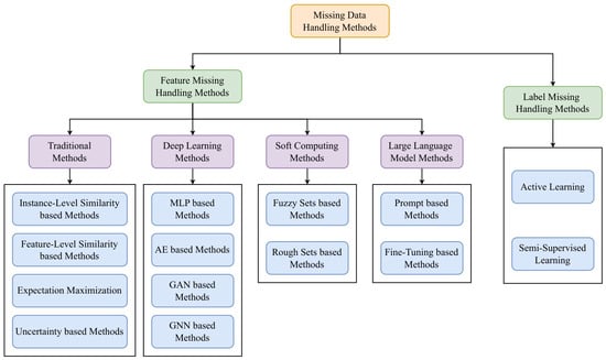
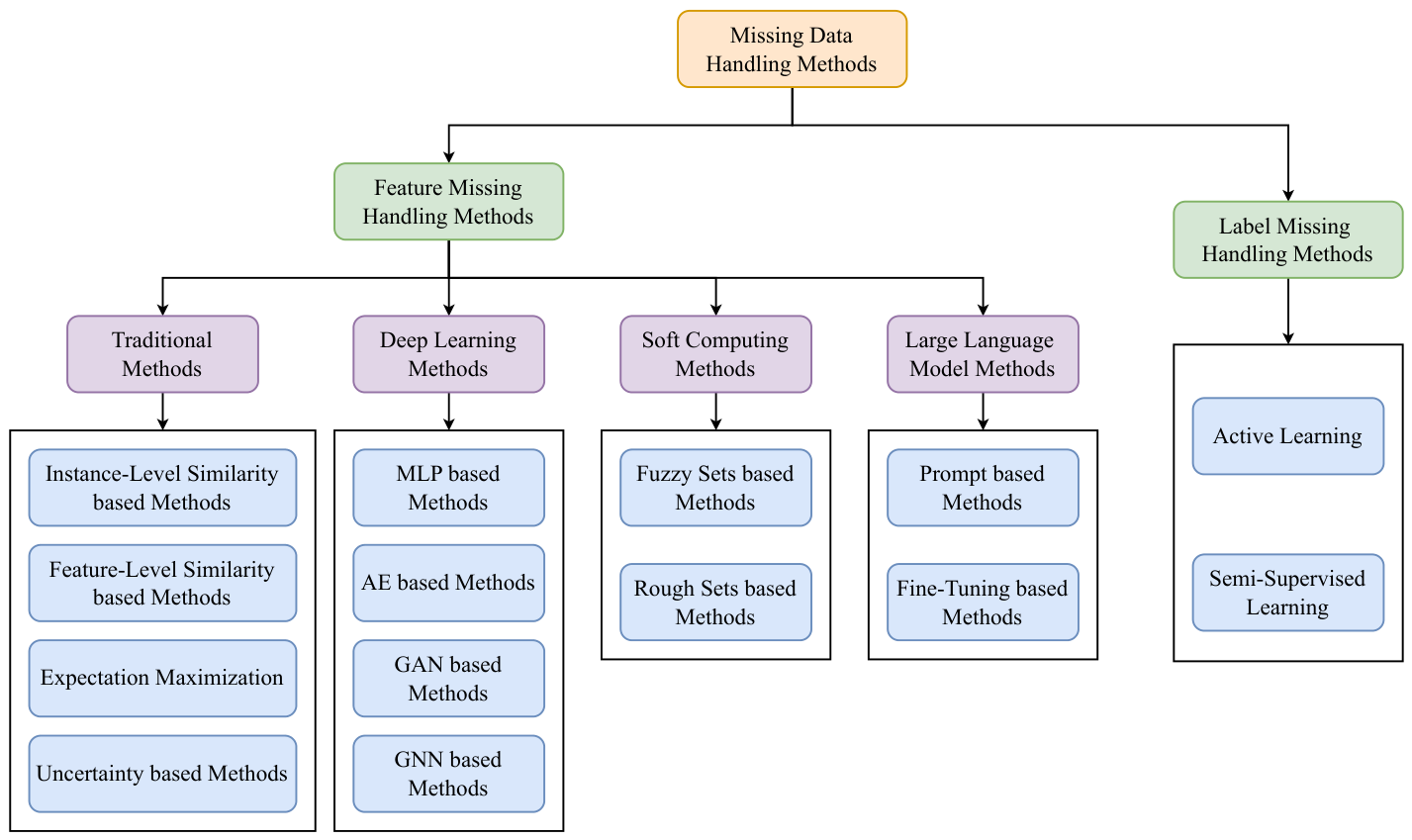
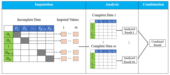
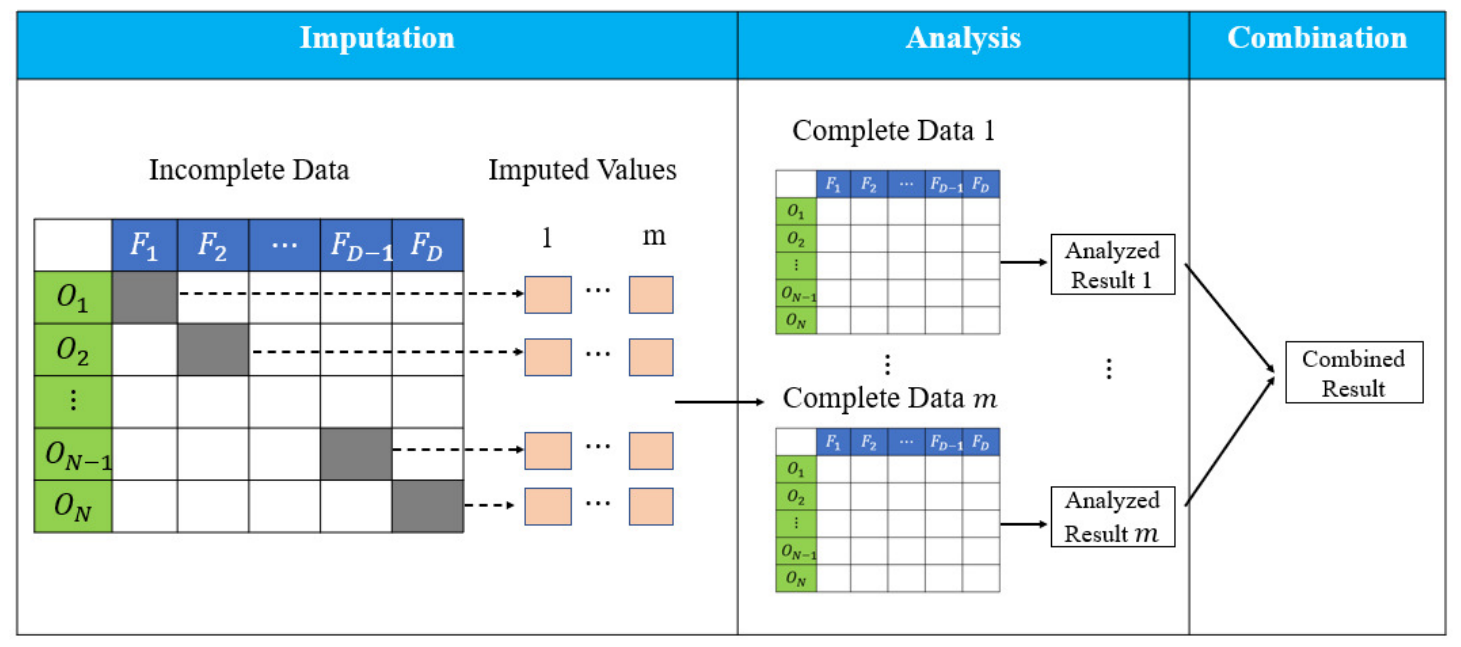
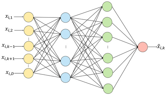
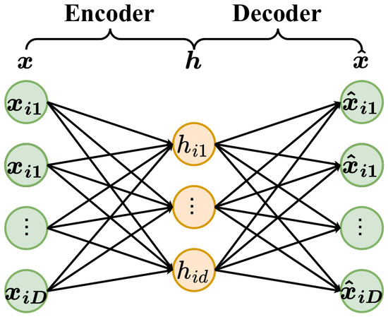
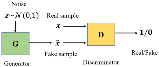
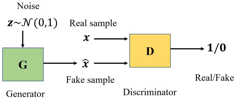
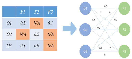
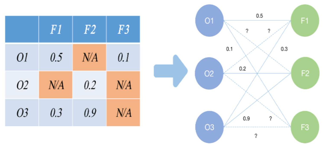
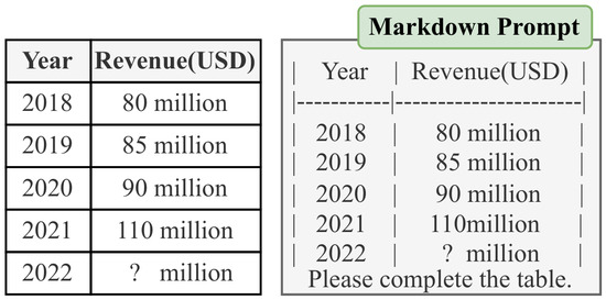
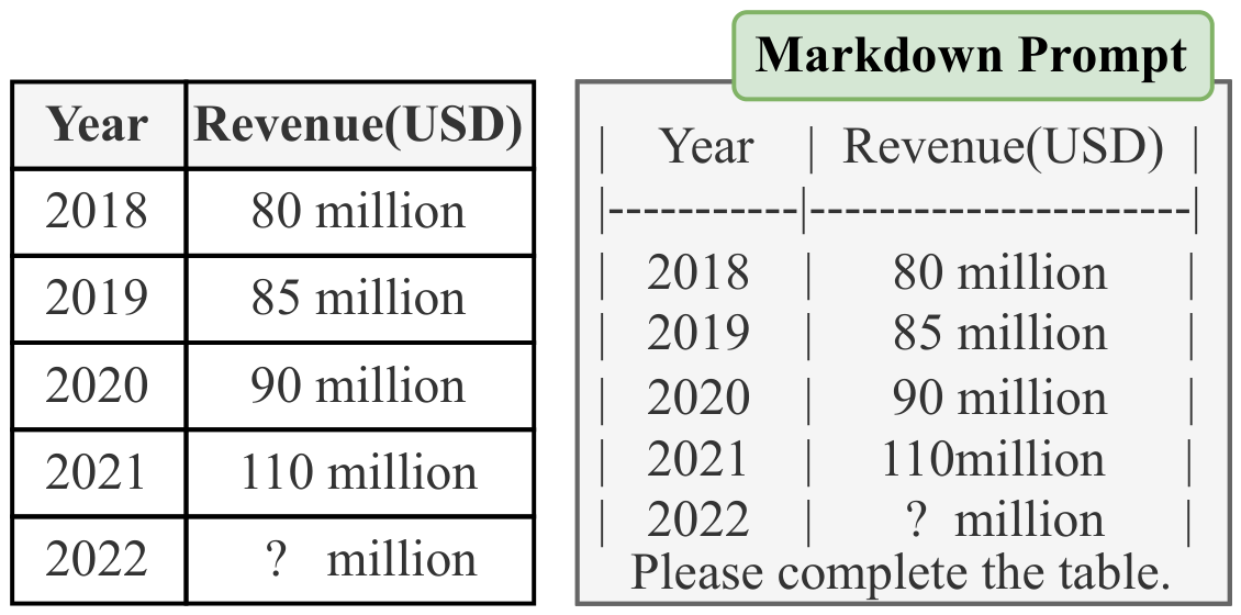

Disclaimer/Publisher’s Note: The statements, opinions and data contained in all publications are solely those of the individual author(s) and contributor(s) and not of MDPI and/or the editor(s). MDPI and/or the editor(s) disclaim responsibility for any injury to people or property resulting from any ideas, methods, instructions or products referred to in the content. |
© 2026 by the authors. Licensee MDPI, Basel, Switzerland. This article is an open access article distributed under the terms and conditions of the Creative Commons Attribution (CC BY) license.