


Abstract
Continuous optimization now draws on a large and growing number of competing metaheuristic families, including differential-evolution lineages, covariance-matrix adaptation strategies, swarm-intelligence methods, and simulated annealing, yet no single method dominates across problem classes, a consequence of the No Free Lunch theorem. This motivates algorithm selection: choosing, for an unseen problem, the method most likely to perform best. Building on the OptimSolution framework, we assemble a headless, reproducible batch-execution pipeline coupled with Exploratory Landscape Analysis (ELA), enabling large-scale, statistically grounded benchmarking together with feature-based meta-learning. We evaluate a set of optimizers of comparable overall strength, drawn from distinct algorithmic families, across a broad benchmark suite spanning classical scalable functions and established competition test suites, under a consistent multi-run evaluation protocol. A Random Forest classifier trained on ELA features, validated under a Leave-One-Problem-Out cross-validation scheme, is shown to predict the best-performing optimizer for a previously unseen problem substantially more accurately than the naive Single Best Solver (SBS) baseline, closing a meaningful share of the gap toward the oracle Virtual Best Solver (VBS). Family-level analysis further shows that structured competition benchmarks and classical scalable functions tend to be won by different solvers, confirming that the underlying selection problem is genuine rather than trivial. These results indicate that landscape-aware selection can meaningfully outperform naive strategies when the candidate methods are drawn from heterogeneous algorithmic families of comparable strength.
1. Introduction
Continuous global optimization is a core computational task across nearly every quantitative discipline, from engineering design to the tuning of machine-learning models. Over the past three decades, the algorithmic community’s response to this need has been extraordinarily prolific: alongside classical evolutionary algorithms [1], the literature now offers entire families of population-based metaheuristics with distinct search mechanisms. Differential Evolution (DE) [2] gave rise to a long lineage of adaptive variants built around success-history parameter control and archive-based mutation, including JADE [3], SHADE [4], L-SHADE [5], and jSO [6]. Evolution strategies gave rise to the Covariance Matrix Adaptation Evolution Strategy (CMA-ES) [7], which adapts a full covariance model of the search distribution rather than perturbing individual variables independently. Swarm intelligence contributed Particle Swarm Optimization [8], Ant Colony Optimization for continuous domains [9], and, more recently, nature-inspired variants such as the Grey Wolf Optimizer [10]. Physics-inspired approaches such as Simulated Annealing [11] remain in wide use as a comparatively low-cost baseline. Each of these families embodies a different bias about how the search space should be explored and exploited, and new variants within each family continue to appear every year, making the practical choice of “which method to use” increasingly difficult rather than easier.
This proliferation is not incidental. The No Free Lunch theorem for optimization [12] formally establishes that, averaged over the space of all possible objective functions, no single optimizer can outperform any other: elevated performance on one class of problems is necessarily offset by inferior performance elsewhere. In practice this means that the “best” algorithm for a given task is contingent on the structure of the problem itself: its modality, separability, ruggedness, and the presence of plateaus or deceptive basins of attraction. The theorem’s averaging is taken over the entire, largely unstructured space of conceivable objective functions, so it does not preclude one method from being reliably better on the much narrower, structured subset of problems that arise in practice. It does, however, remove any theoretical guarantee that a single method will do so, which is precisely why an empirical, data-driven selection procedure of the kind developed here has scientific value. The natural response is therefore not to search for a universally superior algorithm, but to select, for a given unseen problem, the method most likely to perform well on it: the algorithm selection problem, originally formalized by Rice [13] and later surveyed extensively from a meta-learning perspective [14,15]. Exploratory Landscape Analysis (ELA) [16] operationalizes this idea for continuous black-box optimization: a modest sample of the search space is used to compute a compact set of numerical descriptors, related to convexity, level-set structure, local-versus-global information, and similar properties, that summarize how difficult or structured a landscape is, without requiring the objective function to be evaluated exhaustively. Coupled with supervised machine learning, ELA features have been shown capable of predicting which solver from a portfolio is likely to perform best on a new problem instance, closing part of the gap between naive and oracle solver selection [15,17,18,19], and this line of work has been placed within the broader landscape of algorithm-selection methods for black-box continuous optimization in dedicated surveys [20,21,22].
Realizing this landscape-aware selection pipeline in practice is largely an infrastructural problem: it requires (i) a means of running many (method, problem, dimension) combinations reproducibly, (ii) a statistically sound procedure for deciding which method actually “won” each combination, and (iii) an integrated mechanism for sampling problem landscapes and extracting ELA features at scale. In this work we build on the OptimSolution framework [23] and assemble around it a headless, batch-execution pipeline coupled with an ELA extraction stage, producing large, reproducible meta-optimization datasets through four stages: batch execution and statistical ranking, including Friedman omnibus testing [24] and Holm-corrected [25] pairwise Wilcoxon signed-rank tests [26], following established practice for comparing evolutionary and swarm-intelligence algorithms [27,28,29]. The pipeline then performs landscape sampling and ELA feature computation [16], and, finally, it trains a landscape-aware selection model with a Random Forest classifier [30].
The purpose of this paper is to demonstrate, using this pipeline, that a machine-learning model trained on landscape features can predict which optimizer will perform best on a previously unseen problem more accurately than the simplest sensible baseline, always recommending the single method with the best average performance overall, or Single Best Solver (SBS), and doing so with a degree of rigour that makes the comparison meaningful. For this comparison to be genuine rather than trivial, the candidate methods must be of comparable overall strength: pairing one markedly strong solver against several markedly weaker baselines collapses the meta-learning task into a near single-label classification problem, in which no model, however well designed, can outperform the naive SBS baseline by a meaningful margin. We therefore evaluate eight optimizers of comparable overall strength, drawn from four distinct algorithmic families (DE-lineage, CMA-ES, swarm intelligence, and simulated annealing), over 97 (problem, dimension) instances spanning classical scalable functions and the CEC2017 [31] and CEC2022 [32] competition benchmark suites. The novelty of this work is therefore threefold: (i) an explicit methodological argument, together with its empirical confirmation, that the algorithm-selection problem is only genuine, and only worth learning, when the candidate methods are of comparable strength and drawn from heterogeneous algorithmic families; (ii) a large, reproducible meta-optimization dataset assembled around the OptimSolution framework [23], spanning 97 (problem, dimension) instances and eight optimizers; and (iii) a statistically rigorous evaluation of the resulting landscape-aware model, benchmarked under Leave-One-Problem-Out cross-validation against both the naive SBS baseline and the oracle Virtual Best Solver (VBS), quantifying not just whether landscape awareness helps but how much of the achievable performance gap it actually closes.
The remainder of this paper is organized as follows. Section 2 describes the methodological pipeline built around the OptimSolution framework, covering batch execution and Exploratory Landscape Analysis, at the level of what it enables scientifically. Section 3 details the experimental design adopted for the large-scale study: the eight optimizers and their algorithmic families, the benchmark problems drawn from classical, CEC2017, and CEC2022 suites, and the evaluation protocol. Section 4 presents the results of the experiment: per-method statistical rankings, family-level specialization patterns across benchmark suites, and the Leave-One-Problem-Out accuracy of the landscape-aware selection model relative to the SBS and VBS baselines. Section 5 discusses the practical implications and limitations of these findings, including the effect of label tie-breaking on the reported results. Section 6 concludes the paper.
2. Framework Extensions: Headless Batch Execution and Landscape Analysis
Realizing the landscape-aware selection pipeline introduced in Section 1 required extending the OptimSolution framework [23] along three complementary axes: a way to execute a large numbers of (method, problem, dimension) combinations unattended and reproducibly, a principled statistical procedure for turning raw per-combination performance into a labelled meta-dataset, and a mechanism for sampling each problem’s landscape and exporting it for downstream feature extraction. This section describes what each addition does at the methodological level.
Batch execution is driven by a compact specification that defines, for a given experiment, the optimizers, benchmark problems, and dimensions to combine. Two complementary specification styles are supported: a full Cartesian product over methods, problems, and dimensions, and an explicit, sparse list of individual (method, problem, dimension) triples, the latter allowing an existing experiment to be extended incrementally without re-running combinations already completed. Each combination is executed as an independent, seeded run producing a standardized per-combination summary. These summaries are subsequently merged, by column name rather than by raw file order, into a single master table. This master table then passes through a statistical ranking stage that, for every (problem, dimension) group, determines each method’s rank, identifies the group’s best-performing method, and tests whether the differences between methods are large enough to be meaningful: a Friedman omnibus test across all methods, followed by pairwise Wilcoxon signed-rank tests with Holm correction for multiple comparisons. The Friedman test is a non-parametric analogue of repeated-measures analysis of variance: it ranks the methods separately within every (problem, dimension) group and asks whether the resulting average ranks differ more than would be expected by chance alone. When it indicates that they do, the Wilcoxon signed-rank test is used to compare two methods at a time, by ranking the magnitude of their paired performance differences across groups, and the Holm correction lowers the significance threshold required of each individual pairwise test to control the overall risk of a false positive that grows as more pairs are tested simultaneously. It is this ranking stage that turns raw performance numbers into the labelled meta-dataset used to train the selection model evaluated in Section in the associated tables.
In parallel, a landscape-sampling stage draws a fixed budget of points from each problem’s true, declared search bounds, using the same initialization procedure, uniform, Latin-hypercube, or Halton, already used to seed every optimizer in the framework, so that the sample is drawn under exactly the assumptions the optimizers themselves operate under. The problem’s real objective function, not a surrogate, is evaluated at each sampled point. Sample size follows the convention established in the Exploratory Landscape Analysis literature [16] of tens to a few hundred points per dimension: the pipeline draws exactly 100 samples per problem dimension for every instance, using each problem’s declared dimension as listed in Table 1. For the classical Powell function, this declared dimension is not the same one the optimizers themselves run at, as Section 3 explains and Section 5 discusses further. The resulting points and their function values, together with each problem’s declared modality and separability, are exported for feature extraction. Computing the actual ELA descriptors from this sample, distributional statistics, meta-model fit quality, information-content and nearest-better-clustering measures, and level-set classification errors, corresponding to the feature families is deliberately delegated to the established pflacco library [33] rather than re-implemented, so the study relies on independently validated statistics [34] rather than a bespoke reimplementation.
Table 1.
Benchmark problem suite used in the large-scale experiment: 35 problems (16 classical scalable functions, 11 CEC2017, 8 CEC2022) evaluated at the dimensions listed, for a total of 97 (problem, dimension) instances.
To make the pipeline’s inputs, preprocessing, and evaluation protocol fully explicit alongside the descriptive account above, Figure 1 separates the pipeline into two phases with very different computational costs: an OFFLINE phase (Stages 1–4), run once over the 35 benchmark problems to produce and validate a trained model, and an ONLINE phase, run once per new, unseen problem to obtain a recommendation from that already-trained model without running any of the eight candidate optimizers on it. The online phase only draws a landscape sample and computes ELA features from it, orders of magnitude cheaper than running even a single optimizer to convergence, let alone all eight.
Figure 1.
The landscape-aware selection pipeline, separated into an OFFLINE phase (training and Leave-One-Problem-Out validation over the 35 known benchmark problems) and an ONLINE phase (algorithm selection for a single new, unseen problem, using the model already trained offline). The dashed arrow indicates that the deployed model is reused as is, with no retraining per query. Note: the 35-fold LOPO loop (Stage 4) exists purely to produce an honest, out-of-fold accuracy estimate None of the 35 fold-specific classifiers is the one actually deployed—the deployed model (right) is a single Random Forest fit once on all 97 instances.
The feature set consists of 53 numeric ELA descriptors per (problem, dimension) instance, computed by pflacco [33] from the same 100xD-point landscape sample described above, drawn across six feature families: ela_distr (3 descriptors), ela_meta (9), ela_level (9), nbc (5), disp (16), and ic (5), together with one per-family “costs_runtime” diagnostic column that pflacco reports alongside its descriptors (6 in total, 1 per family). These six runtime columns are retained as ordinary numeric features rather than excluded; The feature-importance ranking as outlined in Section 4 indicates the model does not rely materially on any of them. A small number of features take NaN or infinite values for degenerate instances (e.g., the ela_level LDA warning noted during extraction); these are imputed with the corresponding feature’s median value across the dataset before training. No additional feature scaling is applied, since the Random Forest’s axis-aligned splits are invariant to monotonic per-feature rescaling.
The training label for a (problem, dimension) instance is constructed in two stages. First, the set of tied best-performing methods (those attaining is_best = 1 in the Stage 1 ranking) is fixed once, since it depends only on the batch/ranking stage and not on any tie-break policy. Second, because a standard multi-class classifier requires one canonical label per instance, ties are broken in favour of whichever tied method has the better average rank, computed, within each Leave-One-Problem-Out fold, from that fold’s training problems only (Section 5 discusses why this must exclude the held-out problem, and the consequence of getting it wrong). Evaluation itself remains lenient throughout: a prediction is scored correct if it names any member of the tied set, not only the canonical label chosen for training.
The Random Forest itself uses scikit-learn’s default splitting criterion with 200 trees, maximum depth 4, a minimum of one sample per leaf, and balanced class weighting, fit independently within each of the 35 Leave-One-Problem-Out folds purely for evaluation.
None of these 35 fold-specific classifiers is the model actually used for algorithm selection: the deployed model is a separate, final fit (300 trees, otherwise the identical configuration) on all 97 instances, using the analogous, full-dataset tie-break for its own training labels; this same final fit also yields the Gini feature importances reported in Section 4.
The labelled performance table and the extracted landscape features are finally joined on (problem, dimension) and used to train a Random Forest classifier [30]. A Random Forest is an ensemble learner that trains a large number of individual decision trees, each on an independently resampled subset of the training data and a randomly restricted subset of the available features, and it combines their predictions by majority vote. A single decision tree classifies an instance by applying a sequence of threshold tests on individual input features, branching at each step until it reaches a leaf that assigns a class label, in this study, the identifier of the optimizer predicted to perform best. Averaging over many such trees, each fit to a slightly different view of the data, reduces the variance associated with any one tree’s idiosyncratic splits without materially increasing bias, which is why Random Forests are a standard, well-validated choice for tabular classification problems of the kind faced here. This model is evaluated in Section 5, following the Leave-One-Problem-Out protocol standard in the algorithm-selection literature [18]. Under this protocol, every instance belonging to a given problem, across all of its evaluated dimensions, is withheld from training as a single block, and the trained model is then asked to predict the best optimizer only for those withheld instances, before the process repeats with a different problem held out. This is a substantially stricter test than an ordinary random train and test split, since it guarantees that the model never benefits from having already seen a different dimension of the very problem family it is being asked to generalize to, which is the failure mode a random split would not catch.
3. Experimental Design
All eight optimizers evaluated in this study were implemented in C++17 within the open-source OptimSolution framework [23] developed by Vasileios Charilogis and publicly available at https://github.com/charilog/optimsolution (accessed 14 August 2026). All experiments were compiled and executed under Debian 12.12 with GCC 13.4, on a workstation equipped with an AMD Ryzen 9 9950X3D processor (16 cores, 32 threads) and 64 GB of DDR4 memory. All eight methods were implemented natively within this same C++ codebase, rather than invoked through each method’s original, and often differently implemented, reference code.
Table 1 lists the 35 benchmark problems underlying the study, spanning classical scalable functions and the CEC2017 and CEC2022 competition suites, together with the dimensions at which each was evaluated.
Every (method, problem, dimension) combination was run under a single, common protocol. Each run initialized its population from a uniform distribution over the problem’s declared bounds, using a default population size of 100 agents except where a method’s own published design specifies a different value, and was allotted an evaluation budget of 10,000 function evaluations, where D is the problem dimension, terminating once that budget was exhausted. One problem is an exception to this rule as stated: the classical Powell function is defined in blocks of four variables, so its implementation pads the declared dimension up to the next multiple of four before allocating the evaluation budget, meaning the three Powell instances reported as in Table 1 actually run, and receive their evaluation budget, at . All other 34 problems use the declared dimension exactly. This padding is internal to the optimization stage only; its consequence for the landscape-sampling stage described in Section 2 is discussed in Section 5. For every method, the parameter values recommended in the algorithm’s original publication were retained rather than re-tuned for this benchmark, so that reported performance reflects each method’s published default configuration rather than a benchmark-specific tuning advantage. Each combination was repeated for 30 independent runs, with per-run seeds deterministically derived from a common base seed (4242), making the entire experiment exactly reproducible. A run was counted as successful when it reached within of the problem’s target value. The resulting per-instance success rate is the quantity reported as themean success rate in Table 2 and Table 3.
Table 2.
Friedman-based ranking and performance summary across all 97 (problem, dimension) instances (8 methods, 30 runs each). Wins counts the number of instances on which the method achieved the best mean success rate.
Table 3.
Computational cost and behaviour of each optimizer, aggregated over all 97 (problem, dimension) instances from the raw batch-execution log, with all eight methods receiving the same dimension-scaled evaluation budget (Section 3), averaging 275,876 evaluations per instance over the actual mix of dimensions in the benchmark suite. SD success rate reflects consistency across instances. The evaluation budget was exhausted on every run (zero variance) and is identical across methods, so it is not shown as a table column.
4. Experimental Results
Table 2 summarizes the Friedman-based ranking of all eight optimizers across the 97 (problem, dimension) instances, together with the number of instances each method won outright and its mean success rate. The compression-based (sparq) and eigenvector-guided (ea4eig) DE-lineage methods dominate both the rank sum and the win count, but neither approaches an overwhelming majority of wins, indicating that the underlying algorithm-selection problem is non-trivial.
A closer reading of Table 2 shows that the top of the ranking is no longer a two-method contest. sparq retains the best average rank (2.78), but rde and ea4eig follow closely behind (3.01 and 2.85, respectively), and Table 4 shows that rde is not statistically distinguishable from either sparq or ea4eig individually, even though sparq and ea4eig are significantly different from each other. This three-way near-tie at the top reflects rde’s mean success rate of 56.6% under the dimension-scaled evaluation budget every method receives, placing it in direct contention with sparq and ea4eig. cmaes forms a clearly separated fourth tier on its own (average rank 3.96), significantly worse than every member of the top three but significantly better than the band below it. lmcmaes, acor, and gwo occupy a middle band that pairwise Wilcoxon testing cannot statistically separate (average ranks 5.10 to 5.72), none of the three pairwise comparisons among them reaching significance in Table 4. This absence of a significant pairwise difference reflects insufficient evidence, at this sample size, to distinguish these three methods, not a demonstration that their true performance is equal—a stronger claim that would require a dedicated equivalence test rather than a non-significant result. Meanwhile, sa closes the table alone, significantly worse than every other method and, as Table 3 already showed, with a success rate that barely varies across the entire benchmark suite. No single method approaches an overwhelming majority of wins, sparq and rde each win 48 of the 97 instances outright and ea4eig 47, once tied outright victories on easy, near-saturated instances are taken into account. This remains consistent with the paper’s central premise: the eight methods were deliberately chosen to be of comparable strength, and correcting rde’s evaluation budget has, if anything, strengthened that premise rather than weakened it.
Table 4.
Pairwise Wilcoxon signed-rank comparisons between all eight optimizers, with Holm-corrected p-values. n is the number of (problem, dimension) instances on which both methods produced comparable results.
Figure 2 renders the same average-rank values as a bar chart, using a conventional, non-inverted axis: bar height increases directly with average rank, so a taller bar corresponds to a worse (higher) rank, and the chart states this explicitly with its own “Lower bar is better” annotation rather than leaving the direction to be inferred. sparq, highlighted, has the shortest bar but only marginally so: the visual effect makes the four-tier structure discussed above immediately apparent as a staircase, a barely perceptible step separates the three leading, shortest bars (sparq, rde, ea4eig) from one another, a clearer step sets cmaes apart on its own, a further step rises to the three roughly equal mid-table bars (lmcmaes, acor, gwo), and a final, largest step isolates sa’s markedly taller bar at the far right. This kind of visual separation is a useful sanity check before any formal test is run: a benchmark in which the bars formed a smooth, even slope, rather than distinct steps, would suggest a continuum of near-equivalent methods rather than the tiered structure that the Wilcoxon results in Table 4 confirm.
Figure 2.
Average Friedman rank per optimizer across all 97 (problem, dimension) instances (lower is better), corresponding to the values in Table 2.
These same average-rank values are the statistic underlying the omnibus Friedman test that licenses the pairwise comparisons in Table 4. Run on all N = 97 complete groups (every instance for which all eight methods produced a valid result), the Friedman test rejects the null hypothesis that all eight methods perform equivalently decisively (, p ), consistent with the top methods forming a genuinely close-fought upper tier even as the omnibus test remains overwhelmingly significant. This result is what justifies moving from a single omnibus statistic to the 28 individual pairwise tests in Table 4: having established that the eight methods are not all equivalent, the pairwise stage is needed to determine which specific pairs actually differ, rather than assuming every pair does.
Table 3 confirms that every method, including acor and rde, receives the identical dimension-scaled budget of 10,000 times D, averaged to approximately 275,876 evaluations over the actual mix of dimensions in the benchmark suite. With the comparison fair across all eight methods, the remaining columns are informative in their own right. sa’s success rate still has zero standard deviation across all 97 instances, meaning it solves almost exactly the same fraction of its 30 runs on every single problem regardless of landscape, the signature of a method whose behaviour is essentially insensitive to problem structure, and it still stands out computationally with a mean iteration time more than three times higher than the next slowest method (cmaes) despite using the least memory of any method tested, consistent with an acceptance-based search that spends its per-iteration cost on repeated candidate evaluation rather than on maintaining auxiliary state. rde now shows the highest peak memory use of any method (52.1 MB), narrowly ahead of lmcmaes and cmaes, consistent with the external archive its success-history mutation strategy maintains alongside a full population. cmaes and lmcmaes remain, as their shared ancestry would predict, close behind rde in memory use, but they diverge sharply in speed: lmcmaes is the fastest method overall per iteration, consistent with its limited-memory design deliberately avoiding the full covariance-matrix factorization that makes standard cmaes markedly slower despite comparable memory use.
Table 3 reports the per-iteration cost for each candidate optimizer, but it does not by itself answer a different, practical question a reviewer raised: how does the wall-clock cost of the landscape-aware selection pipeline itself compare with simply running one or more of these candidates directly, under a comparable budget? We measured this directly, using the framework’s own per-stage timing log. Table 5 reports the wall-clock cost of landscape sampling (Stage 2), ELA feature extraction (Stage 3), and Random Forest training (Stage 4), aggregated over all 97 (problem, dimension) instances; Table 6 reports the corresponding cost of running each of the eight candidate optimizers once, to its full budget, across the same 97 instances, derived analytically from the validated per-iteration timings underlying Table 3 (mean evaluations divided by population size, times mean iteration time). We use this derived figure rather than a freshly re-measured Stage 1 wall-clock time because re-running Stage 1 on an already-complete batch_master.csv only re-executes the fast statistical ranking step and skips the (already cached) optimizer runs themselves, so a fresh Stage 1 timer would understate the true cost of the 8 × 30 × 97 optimizer runs rather than measure it.
Table 5.
Wall-clock cost of the landscape-aware selection pipeline, aggregated over all 97 (problem, dimension) instances, measured directly from the framework’s per-stage timing log. Online inference cost is measured separately, for a single new instance.
Table 6.
Wall-clock cost of running each candidate optimizer once, to its full dimension-scaled budget, across all 97 (problem, dimension) instances, derived from the per-iteration timings underlying Table 3. “Brute-force” totals the cost of running every one of the eight candidates once on every instance, the exhaustive alternative to landscape-aware selection.
Two conclusions follow directly from Table 5 and Table 6. First, ELA feature extraction, not landscape sampling, dominates the pipeline’s offline cost: at 24.9 s per instance it accounts for about 99.7% of the combined Stage 2 + Stage 3 time, while drawing the 100xD-point sample itself costs a fraction of a second. Second, whether landscape-aware selection is worth its cost depends entirely on what it is being compared against. Against the exhaustive alternative, running every one of the eight candidates once to see which wins, it is cheaper: 2421.3 s (Stages 2–3) versus 4272.6 s brute-force, a 43% reduction. Against simply trusting a single, cheap default, however, it is far more expensive: roughly 25 s of offline computation per new problem, against 0.56 s to run sparq (the Single Best Solver baseline, Table 7) or 0.37 s for the cheapest candidate, lmcmaes. The case for paying this cost is therefore an accuracy argument, not a speed argument: it is justified when closing part of the 35.1-percentage-point gap between SBS and the landscape-aware model’s 66.0% accuracy (Table 7) is worth roughly 45–70 times the wall-clock cost of simply running a strong default optimizer once, for instance, because the selected optimizer will itself be run for a much larger downstream budget, or applied repeatedly, amortizing the one-time selection cost. A practitioner who only needs a single, reasonably strong recommendation and cannot amortize this cost is better served by SBS alone.
Table 7.
Leave-One-Problem-Out cross-validated accuracy of the Random Forest landscape-aware selection model, against the naive Single Best Solver baseline and the oracle Virtual Best Solver upper bound, across all 97 (problem, dimension) instances.
On whether the sampling budget can be reused rather than treated as pure overhead, five of the eight candidates in this study, acor, ea4eig, gwo, sa, and sparq, use a population of exactly 100 individuals (Section 3), identical to the number of points drawn for landscape sampling. For these five methods, the landscape sample computed for ELA feature extraction could, in principle, be reused directly as the selected optimizer’s initial population, at no additional function-evaluation cost: the two stages currently draw independent samples of the same size from the same distribution, purely because the pipeline treats landscape analysis and optimization as separate stages. The remaining three methods would benefit only partially: cmaes and lmcmaes use a much smaller, dimension-scaled population (10–15 in this study), so only a subset of the landscape sample would be needed, while rde’s population scales up to several hundred individuals, so the landscape sample alone would not be sufficient and additional evaluations would still be required. The present pipeline does not implement this reuse; doing so would not reduce the ELA extraction cost that dominates Table 5 but would eliminate the separate cost of initializing the selected optimizer for the five methods above, a modest, low-risk optimization left for future implementation work rather than attempted here.
Table 4 reports the full set of pairwise Wilcoxon signed-rank comparisons between the eight optimizers, with Holm-corrected p-values. A total of 5 of the 28 pairs fail to reach significance at : acor vs. gwo, acor vs. lmcmaes, ea4eig vs. rde, gwo vs. lmcmaes, and rde vs. sparq. These five exceptions map exactly onto the tier structure identified in Table 2: two fall within the top tier (rde against ea4eig and against sparq), and three fall within the middle tier (acor against gwo and against lmcmaes, together with gwo against lmcmaes), confirming that the performance differences separating the four tiers from one another are statistically robust, while the differences within each tier are not reliably distinguishable from noise. Of the 28 pairwise comparisons in Table 4, 23 remain statistically significant after Holm correction. The remaining five are the pairs already identified above: acor versus gwo, acor versus lmcmaes, ea4eig versus rde, gwo versus lmcmaes, and rde versus sparq. Four of these five are among the pairs whose average ranks in Table 2 are closest together (rank gaps of 0.16–0.35), the exception being gwo versus lmcmaes (gap of 0.62); by contrast, the single closest pair overall, sparq versus ea4eig (gap of only 0.07), is nonetheless statistically significant, showing that closeness in average rank does not by itself guarantee non-significance. In practice this means that, within the present benchmark suite, distinguishing acor from gwo, acor from lmcmaes, gwo from lmcmaes, ea4eig from rde, or rde from sparq is not a meaningful sub-problem for a selection model to solve, since the underlying performance data do not support such a distinction. The number of paired instances entering each test (the n column) is not always 97, since the Wilcoxon signed-rank test excludes ties (pairs with identical performance are uninformative for a signed-rank comparison), so pairs involving two closely matched top-tier methods, such as cmaes and lmcmaes, contribute noticeably fewer usable comparisons than pairs drawn from more clearly separated methods. Across the 28 pairs, this effective sample size ranges from 62 to the full 97, and the reduction is not merely cosmetic: 3 of the 5 pairs that fail to reach significance, acor versus lmcmaes, ea4eig versus rde, and rde versus sparq, are also among the pairs with the fewest usable instances (88, 70, and 75, respectively), so part of what separates these 3 from the 23 significant pairs may be reduced statistical power rather than a genuinely smaller true effect. The clearest counter-example is cmaes versus sparq, which has the smallest n of all 28 pairs (62) yet remains highly significant, showing that a small n does not by itself explain a non-significant result here, but it does mean the 5 non-significant pairs should not be read as demonstrating equivalence with the same confidence throughout.
Figure 3 adds two things that the summary statistics in Table 2 and Table 4 cannot show on their own: the full shape of each method’s rank distribution, and a visual accounting of every pairwise test at once. The boxes for sparq, ea4eig, rde, and cmaes sit low and are comparatively narrow, confirming that all four are not merely better on average but consistently so. By contrast, lmcmaes, acor, and gwo each display boxes and whiskers that span nearly the entire rank scale, from close to rank one to close to rank eight, indicating that every method in this middle band wins decisively on some instances and loses badly on others. This instance-by-instance volatility, invisible in an average-rank table, is direct visual evidence for the family-level specialization discussed in the abstract and revisited in Table 8. sa stands apart with a box compressed near the top of the scale and almost no vertical spread, the visual counterpart of the zero-variance finding for sa already noted in Table 3. The dense stack of significance brackets across the upper part of the plot reflects the fact that all 28 pairwise comparisons are drawn, not a selected subset. Against that density, five brackets are marked not significant, matching exactly the five pairs identified in Table 4, and each connects two methods within the same tier rather than crossing between tiers, which is the pattern a correctly tiered ranking should produce.
Figure 3.
Per-method rank distribution across all problem instances, with pairwise Wilcoxon significance brackets. Asterisks (*) denote a statistically significant pairwise difference (Holm-corrected ); ns denotes a non-significant pair, the five listed in Table 4.
Table 8.
Percentage of instances won outright by each method within each benchmark suite (CEC2017, n = 33, CEC2022, n = 16, Classical, n = 48), computed from the is_best indicator in the raw batch results. Percentages within a column need not sum to 100 because a tied outright win is counted for every method sharing it.
The composition of Table 9 is itself an empirical finding. Gini importance measures how much, on average across every tree in the forest, a feature contributes to reducing class impurity at the nodes where it is chosen to split the data, so a larger value identifies a feature the model relies on more heavily when deciding which optimizer is likely to win. The dispersion family contributes the most, four of the ten most important features; ela_meta contributes three, ela_level two, and ic.m0 rounds out the list as the sole individual representative of a fourth family. The ela_level family (mmce_lda_50, mmce_lda_25) measures how accurately a simple linear classifier, linear discriminant analysis, can separate the better-performing fraction of sampled points from the rest at a given quantile threshold, and it takes the top spot in the ranking, indicating that Random Forest relies heavily on how cleanly a landscape’s good and bad regions can be linearly separated. The ela_meta family contributes an equally large share: two variants of the adjusted R-squared of a linear model fit to the sampled points, with and without pairwise interaction terms, and the ratio between that model’s largest and smallest coefficient magnitudes, together capturing how close the landscape is to being linear and how unevenly it responds to different variables. The dispersion family (disp) contributes four features, the mean and median version of the same comparison at both the 2% and 10% quantile thresholds, each comparing the spread of the best-performing sampled points to the spread of the full sample: a direct measure of whether good points cluster together, a funnel-shaped landscape, or are scattered throughout the search space. ic.m0, from the information-content family, measures the proportion of essentially flat steps along a random walk across the landscape and is the fourth most important predictor overall. Taken together, the model’s strongest predictors describe how separable, how linear, how funnel-shaped, and how flat a landscape is, four largely independent structural properties the trained Random Forest relies on most heavily when predicting algorithm selection on this suite. Gini importance reflects how useful a feature was for splitting nodes in the fitted trees, a measure of predictive association within this particular model, not a causal test of which landscape properties actually determine optimizer performance; establishing a causal role would require a separate, targeted analysis, such as controlled ablation of individual landscape properties, beyond the scope of this study.
Table 9.
Ten most important ELA features for the Random Forest landscape-aware selection model, ranked by Gini importance, with a plain-language gloss of what each feature measures.
For completeness, and to give the full, reproducible feature specification a reviewer or future user of this pipeline would need, Table 10 lists all 53 ELA features used to train the Random Forest, grouped by feature family and ranked by Gini importance, extending the top-10 view already given in Table 9. A total of 6 of the 53 (1 per family) are the “costs_runtime” diagnostics discussed in Section 2; 5 of the 6 rank among the 10 least important features, and the exception, disp.costs_runtime, still ranks only 35th of 53, consistent with the model deriving its predictive signal overwhelmingly from landscape structure rather than incidental computation cost.
Table 10.
Complete list of all 53 ELA features used to train the Random Forest, grouped by feature family and ranked by Gini importance (descending).
Table 10’s Gini importance ranking identifies which features the trained Random Forest relies on, but, as Section 4 already notes, this reflects association within one fitted model rather than a controlled test of necessity or sufficiency. Table 11 reports exactly such a test: the same fold-safe Leave-One-Problem-Out protocol, repeated once per ELA feature family, once with that family excluded from the other 52 features (a necessity check), and once with only that family’s features available (a sufficiency check), holding every other aspect of the pipeline, folds, tie-break policy, and classifier hyperparameters, fixed.
Table 11.
Feature-group ablation (Reviewer 2, comment 4): Leave-One-Problem-Out lenient accuracy when each ELA feature family is excluded (necessity) or used alone (sufficiency), against the full, 53-feature model (Table 7). Every row uses the identical fold-safe LOPO protocol, differing only in which feature columns are available to the classifier.
Two patterns stand out. First, no single family is strictly necessary: excluding any one family costs at most 3.1 percentage points (ela_meta), and excluding ela_level, nbc, or disp each leaves accuracy unchanged or improves it (by 1.0, 1.0, and 6.2 points, respectively), indicating the six families carry substantially redundant signal rather than each contributing an indispensable, disjoint piece. Second, the families are far from equally sufficient on their own: ela_meta alone, using only 10 of the 53 features, reaches 70.1%, 4.1 points above the full model and the only single family whose accuracy alone exceeds it; ela_level alone exactly matches the full model (66.0%), while disp, ic, and nbc alone all fall below it. At the other extreme, ela_distr alone, with only four features, collapses to 47.4%, an 18.6-point drop, though still comfortably above the 30.9% Single Best Solver baseline (Table 7). This concentration of predictive signal in ela_meta is consistent with, and independently corroborates, the Gini importance ranking in Table 9, where ela_meta features occupy 3 of the top 10 positions, using a methodology (ablation) that does not share any of the assumptions behind Gini importance. The ablation evidence for ela_level is more mixed: it contributes the single most important individual feature by Gini importance, and used alone it matches the full model’s accuracy, but excluding it entirely does not hurt accuracy either, suggesting its signal is at least partially redundant with the other families, particularly disp, whose own exclusion improves accuracy the most of any single family.
That four configurations, minus disp, minus ela_level, minus nbc, and only ela_meta, all outperform the full 53-feature model is itself informative: with only 97 training instances, adding features beyond a certain point appears to dilute rather than help the Random Forest, consistent with a mild curse-of-dimensionality effect rather than every additional feature contributing genuine signal. This suggests that feature selection, for instance, restricting the model to the ela_meta family alone or excluding disp, is a concrete, testable direction for improving on the 66.0% headline accuracy in future work, rather than a claim we pursue further in the present study.
A further contribution of Reviewer 2, comment 4 asks for a comparison with alternative selection models to establish whether the Random Forest used throughout this study is actually the strongest available choice, rather than an unexamined default. Table 12 reports three alternatives, an RBF-kernel support vector machine, gradient boosting, and multinomial logistic regression, each run through the identical fold-safe Leave-One-Problem-Out protocol, on the same 53 features and the same folds as the Random Forest, differing only in the classifier itself and, for the two scale-sensitive alternatives, whether features are standardized (a scaler fit on each fold’s training data only, to avoid the same kind of leakage Section 5 discusses for the tie-break policy).
Table 12.
Comparison with alternative selection models (Reviewer 2, comment 4): Leave-One-Problem-Out lenient accuracy for three alternative classifiers against this study’s Random Forest (Table 7), all on the same 53 features and folds. “Scaled features” indicates a per-fold StandardScaler fit on training data only.
This study’s Random Forest is, in fact, the strongest of the four: gradient boosting, the closest competitor, trails by 2.1 percentage points, and the two scale-sensitive alternatives trail by considerably more (8.2 and 5.2 points for SVM and logistic regression, respectively). All four, however, comfortably exceed the 30.9% Single Best Solver baseline (Table 7), so the choice of classifier changes how much of the SBS-to-VBS gap is closed, not whether landscape-aware selection helps at all: even the weakest alternative, SVM, still closes nearly 40% of that gap (Random Forest itself closes just over half, 50.7%, Table 7). The two tree-based ensembles (Random Forest, gradient boosting) both outperform the two scale-sensitive alternatives (SVM, logistic regression), consistent with tree ensembles’ well-documented robustness on small, tabular datasets of exactly this size; logistic regression in turn outperforms the kernel-based SVM by three percentage points, though with only 97 instances this specific ordering between the two scale-sensitive methods should be read as suggestive rather than definitive. We did not tune any of the three alternatives beyond their scikit-learn defaults (Section 4 reports the Random Forest’s own hyperparameters, which were similarly taken from common practice rather than tuned for this dataset); a fully tuned comparison across classifiers, like the feature-selection direction noted above, is left for future work rather than pursued here.
The ranges in Table 13 confirm that these ten features are doing genuine discriminative work rather than taking a nearly constant value across the suite. ela_meta.lin_simple.coef.max_by_min, the ratio between a linear model’s largest and smallest coefficient magnitudes, shows by far the widest range of the ten, from under three to over ten thousand, reflecting how starkly some landscapes respond to one variable far more than another while others respond almost uniformly across all variables. The four dispersion features (disp.diff_mean_02, disp.diff_median_02, disp.diff_mean_10, disp.diff_median_10) show the next widest ranges, each spanning several hundred units from negative to positive. Because these features are computed directly in the objective function’s raw fitness units rather than as a scale-invariant statistic, part of this spread reflects the very different fitness-value scales across the benchmark suite, composition and hybrid CEC functions in particular can carry offsets in the thousands, as well as genuine differences in landscape shape. Both ela_meta adjusted-R-squared features span almost their entire possible range, from close to zero (a landscape a linear model cannot fit at all) to close to one (a landscape that is nearly linear), directly evidencing that the benchmark suite mixes structurally simple and structurally complex problems rather than a narrow band of similarly-shaped instances. ic.m0 occupies by far the narrowest band of the ten, across all 97 instances (0.53 to 0.67), which is expected since this feature, derived from the sign pattern of consecutive fitness differences along a sampling path rather than from the objective function’s raw magnitude, is scale-invariant by construction. Its position as the fourth most important predictor in Table 9 therefore reflects small but consistently informative differences rather than dramatic swings between problems. The level-set classification-error features (ela_level) occupy low-to-moderate values throughout, generally under 0.5, but with standard deviations reaching roughly half of their mean values, a degree of spread large enough to help explain why this family, together with ela_meta and disp, is one of the three largest contributors to Table 9.
Table 13.
Descriptive statistics, across all 97 problem instances, of the ten ELA features identified as most important in Table 9. The wide ranges observed confirm that the benchmark suite samples landscapes of substantially different character rather than near-duplicate instances.
The aggregate rankings in Table 2 average over the entire benchmark suite, and in doing so they can obscure exactly the kind of landscape-dependent behaviour that motivates a learned selection model in the first place. Table 8 breaks the same win data down by benchmark family, and it reveals that the top three methods do not simply trade places, they specialize in substantially different regions of the suite.
rde wins the largest share of instances in both CEC suites, 69.7% of CEC2017 and 62.5% of CEC2022, exceeding even ea4eig’s substantial presence there (48.5% and 56.2%, respectively). The CEC suites include the highest-dimensional problems in the benchmark, consistent with rde’s dimension-scaled evaluation budget giving it the most room to exploit at higher dimension. sparq remains the clear leader on classical scalable functions (83.3%), but the runner-up position there belongs to cmaes (60.4%) rather than to ea4eig, which wins only 45.8% of classical instances despite its strength on both CEC suites, indicating that ea4eig’s advantage is tied specifically to the shifted, rotated, and hybrid or composition structures that characterize competition benchmarks rather than being a general-purpose strength. rde shows the mirror image of this pattern, dominant on the CEC suites but comparatively weak on classical functions (31.2%), a specialization in the opposite direction from sparq’s. This three-way division of labour, rde and ea4eig sharing the structured competition benchmarks between them while sparq leads on classical functions, is the concrete, suite-level evidence behind the abstract’s claim that the underlying selection problem is genuine rather than trivial: a rule that always recommended a single fixed method, however strong on average, would necessarily perform poorly on whichever suite that method does not specialize in, and with three methods genuinely competitive at the top, that rule has three plausible but individually wrong candidates to choose from rather than one. acor shows a modest but roughly even presence across all three suites (15.2% to 20.8%) rather than a specialization of its own, consistent with its middle-tier position in Table 2. gwo remains almost entirely absent from both CEC suites (0.0% on each) while retaining a modest classical presence (18.8%), and sa remains the weakest method throughout, winning essentially nothing on classical functions and only a small share of the CEC suites.
Table 7 reports the paper’s central meta-learning result, the outcome the experimental design described in Section 2 and Section 3 was built to obtain.
Trained on the ELA features described in Section 2 and validated under the Leave-One-Problem-Out protocol described in the same section, so that every dimension of a given problem is withheld from training as a single block, the Random Forest classifier correctly identifies the best-performing optimizer, or one of the tied best, for 66.0% of the 97 held-out instances. This exceeds the Single Best Solver baseline, which within each training fold recommends whichever single method has the best average rank among the remaining training instances, in practice, sparq in the great majority of folds (79 of 97) and ea4eig in the rest (18 of 97), consistent with their standing as the top two methods by average rank in Table 2. The model exceeds this baseline by 35.1 percentage points (30.9%), and closes 50.7% of the gap between that baseline and the oracle Virtual Best Solver’s 100% upper bound, the accuracy a hypothetical selector that always chose correctly would achieve. This margin is neither large nor guaranteed by the experimental design, and that is what makes it informative rather than a foregone conclusion: the eight candidate methods were deliberately chosen to be of comparable strength precisely so that no single method could win outright, so a model that failed to beat SBS under this design would have indicated that the ELA features carry no genuine predictive signal for algorithm selection on this suite. That the model does exceed SBS, without approaching the VBS ceiling, places the result appropriately between the two extremes the introduction identified as the boundaries of a meaningful algorithm-selection experiment, neither trivial, since SBS alone would already be adequate in that case, nor unachievable, since VBS remains a further 34.0 percentage points away. The tie-breaking procedure used to construct training labels, discussed further in Section 5, means this figure is best read as a first, methodologically sound estimate of what landscape-aware selection can achieve on this suite, rather than as a ceiling on what the approach could ultimately deliver with further tuning.
The 66.0% versus 30.9% comparison in Table 7 is a paired comparison, since both the Random Forest and the Single Best Solver are evaluated on the same 97 held-out instances, which makes McNemar’s test the appropriate significance test. Of the 97 instances, the Random Forest is correct and the Single Best Solver is wrong on 34 instances, while the reverse, the Single Best Solver correct and the Random Forest wrong, never occurs. The exact binomial form of McNemar’s test on this 34-to-0 split is decisively significant (p = 1.2 × 10⁻¹⁰; continuity-corrected , p = 1.5 × 10⁻⁸), confirming that the Random Forest’s advantage over the Single Best Solver baseline is not attributable to chance. Table 14 further reports two class-imbalance-aware metrics computed against the single canonical training label used for each instance (Section 5 discusses how this label is chosen): balanced accuracy, the average per-class recall across the eight optimizers, and macro-averaged F1. Both metrics drop substantially relative to the lenient accuracy reported in Table 7 for the Random Forest (balanced accuracy 33.9%, macro-F1 32.6%), and they drop even further for the Single Best Solver (balanced accuracy 12.5%, macro-F1 9.4%), which by construction can only ever predict sparq or ea4eig and therefore has zero recall on every other class. The Random Forest still outperforms the Single Best Solver by a wide margin on both class-imbalance-aware metrics, but its own per-class recall is zero on the two rarest labels in the training data, cmaes (1 instance) and sa (3 instances): the model never predicts either method, even on the instances where one of them is the actual best performer. This confirms, concretely rather than speculatively, the class-imbalance concern raised in Section 5 that the model’s lenient accuracy is a genuine improvement over the baseline, but it is also, in part, an artifact of the training-label imbalance, and a practitioner relying on this model should not expect it to ever recommend cmaes or sa, regardless of the landscape features of a new problem.
Table 14.
Significance test and class-imbalance-aware evaluation of the Random Forest landscape-aware selection model against the Single Best Solver baseline, computed from the per-instance Leave-One-Problem-Out prediction record underlying Table 7. McNemar’s test on the paired correctness record (34 instances correct for Random Forest and wrong for SBS, 0 the reverse) gives (exact binomial). Balanced accuracy and macro-F1 are computed against the single canonical training label per instance (see Section 5).
5. Discussion and Limitations
Taken together, the results in Section 4 support a coherent picture. The eight optimizers separate into four statistically distinguishable performance tiers rather than a single clear winner, the differences between all but 5 of the 28 pairs of methods are robust to Holm-corrected pairwise testing, the three methods that anchor the top tier divide the benchmark suite between them rather than one simply dominating the others, and a landscape-aware Random Forest model trained on this structure is intended to predict the best-performing optimizer for a previously unseen problem more accurately than the naive strategy of always recommending the same method (Table 7). Each of these findings depends on the others: the four-tier structure establishes that no single method makes the comparison trivial, and the family-level specialization in Table 8 supplies the landscape-dependent signal a selection model could plausibly learn. The accuracy result in Table 7 reflects rde competitive at the top of the ranking (Table 3). The Single Best Solver baseline the model is compared against is, correspondingly, sparq or ea4eig depending on the training fold, the same two methods that lead Table 2 by average rank, since ties in the training labels are broken in favour of whichever tied method has the better overall average rank rather than arbitrarily, as discussed further below. The remainder of this section discusses this and other limitations that qualify how far the picture in this paper should be generalized.
A further methodological question concerns the independence assumption underlying the Friedman and Wilcoxon tests in Table 2 and Table 4, which treat all 97 (problem, dimension) instances as exchangeable blocks. Different dimensions of the same problem are not strictly independent, since they share the same underlying function and are optimized by the same method under the same protocol; a genuinely independent-blocks design would instead treat each of the 35 problems as a single block. As a robustness check, we repeated the ranking analysis with each method’s instance-level rank averaged across all evaluated dimensions of a given problem, and then we re-ranked within each problem, yielding 35 independent blocks (Table 15). The resulting average-rank ordering reproduces the same four-tier structure reported in Table 2, and the Friedman test remains highly significant (, p), compared with , p at the instance level. As expected with fewer, coarser blocks, more pairwise Wilcoxon comparisons lose significance after Holm correction at the problem level (9 of 28, versus 5 at the instance level), reflecting reduced statistical power rather than a qualitative change in the ranking. Critically, the five pairs non-significant at the instance level remain non-significant here, and no pair reverses tier membership. We therefore report the instance-level analysis in Table 2 and Table 4 as the primary result, since it uses the full resolution of the experimental design, while treating Table 15 as confirmation that the tiering it reveals is not an artifact of treating dependent dimensions as independent blocks.
Table 15.
Robustness check: problem-level re-analysis (35 independent blocks, 1 per problem) against the instance-level analysis reported in Table 2 (97 blocks). Problem-level ranks are obtained by averaging each method’s instance-level rank across a problem’s evaluated dimensions, then re-ranking within each problem.
The clearest remaining subtlety concerns how ties were broken when constructing the training labels used to fit the selection model. When two or more methods share the best recorded performance on a given instance, evaluation of the trained model is lenient; a prediction is scored correct if it names any one of the tied methods, but the single label used during training still has to name one representative method. Ties are common in this dataset, roughly half of the 97 instances (50) have more than one method sharing the best recorded performance. Rather than breaking these ties by an arbitrary rule such as alphabetical order, the single training label is chosen as whichever tied method has the best average rank, so the label reflects genuine relative strength rather than an accident of spelling. An earlier version of this pipeline computed that average rank once, globally, over the full 97-instance table, before the Leave-One-Problem-Out loop began, and reused the same preference order in every fold. This let a held-out problem’s own performance data help decide the tie-break preference order used to label the OTHER problems the model was trained on for the very fold being tested on that problem: a narrow but genuine form of train/test leakage, since a training label should never depend on the instance it will later be evaluated against. We thank a reviewer for pointing this out. The fix, applied throughout this revision, computes the tie-break preference order separately inside each fold, from that fold’s training problems only, so the held-out problem never influences any label used to train the model tested on it. A canonical label can therefore now legitimately differ across folds for the same instance: of the 50 tied instances, 22 have a canonical label that alternates between sparq and ea4eig depending on which problem is held out, reflecting how close these two methods’ average ranks are (2.78 and 2.85 in Table 2); the remaining 28 are stable across every fold (19 sparq, 7 ea4eig, 2 rde). This does not affect the fairness of the accuracy figures reported in Table 7 itself, since evaluation credits any tied method equally regardless of which one was chosen as the canonical label for training; what the leakage affected was which instances’ labels a given fold’s classifier was trained on, which in turn affects what that classifier learns to predict. Correcting it lowers the Random Forest’s Leave-One-Problem-Out accuracy from an earlier, leakage-affected 75.3% to 67.0%, subsequently revised once more to the 66.0% now reported in Table 7, the model still exceeds the Single Best Solver baseline by a wide and statistically decisive margin (Table 14 Section 4), but by a smaller, and now leakage-free, margin than originally reported. The same rank-based rule also determines the identity of the Single Best Solver baseline: rather than the most frequent alphabetically tie-broken label, SBS is defined directly from each training fold’s raw performance data as the method with the best average rank in that fold, which is sparq in 79 of the 97 folds and ea4eig in the remaining 18, exactly the two methods that lead Table 2 by average rank; this definition was already computed fold by fold from training data only and is unaffected by the fix above. A residual simplification remains: a single canonical label is still required to train a standard multi-class classifier, so an instance where several methods are genuinely equivalent still contributes one label rather than several. Training the classifier directly on all tied labels as simultaneously correct targets, rather than collapsing them to one before training, remains a natural direction for further refinement.
A second point, raised by a reviewer, concerns the classical Powell function, the only one of the thirty-five benchmark problems whose declared dimension is not the dimension the optimizers actually run at. This is not itself a limitation: as noted in Section 3, Powell’s classical definition requires the dimension to be a multiple of four, so it is a normal and expected property of this particular function, not an artifact of the experimental design, that the optimization stage pads up to before allocating the 10,000 evaluation budget and running the search.
An earlier version of the landscape-sampling stage (Section 2) did not account for this padding correctly. It sampled and evaluated points at the full, padded dimension, exactly matching what the optimizers themselves use, but it exported only the first 10, 30, or 50 of the resulting 12, 32, or 52 coordinates to the ELA feature-extraction stage, discarding the remaining two coordinates of every sampled point. Because Powell’s objective function sums a term over every consecutive block of four variables, it genuinely depends on all of a point’s coordinates, so the exported design matrix for these three instances could no longer determine the exported objective values: for the instance, roughly 28% of the variance in the recorded fitness values came from coordinates that were never written to the file. The resulting ELA features therefore did not describe the landscape the optimizers actually searched, nor even a self-consistent lower-dimensional landscape: they described a design matrix with an unmodelled, unrecorded source of variation built into its own target values. This is a more serious problem than a simple dimensionality mismatch between features and optimizer performance, and it is corrected in this revision.
The fix, applied throughout this revision, exports every sampled point’s coordinates at the same, effective dimension used for sampling and evaluation, so the three affected (problem, dimension) instances now draw 1200, 3200, and 5200 samples (100 times the effective dimension) with 12, 32, and 52 x-columns, respectively, and their ELA features are computed from a design matrix that fully determines the recorded objective values, exactly like every other problem in the suite. We verified this directly: the corrected export files’ objective values are now an exact function of the exported coordinates, and re-running the batch-execution stage reproduces the framework’s own optimizer-performance results (Table 2 and Table 3) numerically identically to the pre-correction run, since fixing the landscape-sampling stage does not touch the optimization stage at all.
Recomputing the three Powell ELA rows and retraining the Random Forest changes the headline Leave-One-Problem-Out accuracy from 67.0% to 66.0% (Table 7), a small, honest shift rather than the negligible one speculated in an earlier draft of this discussion. The change is not confined to Powell’s own three instances, whose predictions, all incorrectly giving ea4eig rather than the actual best, sparq, are themselves unaffected by the fix: because Powell’s corrected features also serve as training data in every fold except the one holding Powell itself out, the fix altered the Random Forest’s decision boundary enough to flip three other instances’ predictions (cec2017f14 at , cec2022hybrid2 at , and salomon at ; two from correct to incorrect and one from incorrect to correct, a net change of one instance). This ripple effect, though small, is itself informative: it illustrates concretely why the tie-breaking leakage fix earlier in this section and the present correction both matter beyond the handful of instances each directly touches, since every training instance’s features and labels can influence predictions for problems elsewhere in the suite. Every downstream table and figure derived from the Random Forest, Table 7, Table 9, Table 10, Table 11, Table 12, Table 13 and Table 14, reflects the corrected data throughout this revision. The affected Powell instances remain identifiable directly from Table 1.
A second limitation concerns the coverage of the CEC2022 suite. The experiment includes eight of the twelve functions in the official CEC2022 bound-constrained benchmark, spanning its unimodal, basic, hybrid, and composition categories, but it omits four functions, three composition functions, and one hybrid function that were not available in the framework’s problem set at the time the experiment was run. The eight included functions still span every structural category the official suite is designed to cover, so the qualitative CEC2022 finding in Table 8 is unlikely to be an artifact of this omission, but a reviewer comparing directly against studies that report all twelve official functions should be aware that the present CEC2022 results are not a complete replication of that benchmark.
Finally, several aspects of the meta-learning stage itself were held fixed rather than tuned or independently verified against alternatives, for reasons of scope rather than principle. The Random Forest’s hyperparameters, the number of trees and the maximum tree depth, were set to values commonly used in the algorithm-selection literature rather than optimized for this specific dataset through a nested cross-validation search, so the figures in Table 7 should be read as an achievable accuracy under a reasonable, literature-consistent configuration rather than the best accuracy this approach could in principle reach. A paired McNemar’s test on the per-instance predictions underlying Table 7 confirms that this advantage is statistically decisive rather than attributable to chance (Table 14, Section 4), which also reports balanced accuracy and macro-F1 to address class imbalance directly rather than relying on the lenient accuracy figure alone. The training labels are also imbalanced, sparq, rde, and ea4eig together accounting for the large majority of best-performing outcomes (Table 2), a three-way imbalance, which means a portion of any reported accuracy could in principle be attributable to the model learning this base-rate imbalance rather than genuine landscape-feature structure, a concern the family-level specialization result in Table 8 partially, but not completely, addresses. Table 14 confirms this concretely rather than merely as a theoretical possibility: the trained model has zero recall on cmaes and sa, the two rarest training labels, and never predicts either method regardless of a new problem’s landscape features. Extending the evaluation with a class-imbalance-aware training procedure, such as class-weighted or resampled Random Forests, remains a natural next step that would strengthen, without altering, the qualitative conclusion drawn here. Comparing alternative classifiers trained on the same ELA features, by contrast, is no longer future work: Section 4 (Table 12) now reports it directly, finding the Random Forest used throughout this study to be the strongest of the four models compared.
6. Conclusions
This paper set out to demonstrate that a machine-learning model trained on landscape features can predict the best-performing optimizer for a previously unseen problem more accurately than the simplest sensible baseline, and to do so under an experimental design rigorous enough for that comparison to be meaningful rather than assumed. Working with the OptimSolution framework [23], we assembled a batch-execution and landscape-sampling pipeline, evaluated eight optimizers of comparable overall strength drawn from four distinct algorithmic families across 97 (problem, dimension) instances spanning classical, CEC2017, and CEC2022 benchmarks, and trained a Random Forest classifier on the resulting Exploratory Landscape Analysis features.
The results support three main conclusions. First, the eight methods separate into four statistically distinguishable performance tiers, confirmed by a Friedman omnibus test and Holm-corrected pairwise Wilcoxon comparisons, rather than collapsing into either a single dominant method or a set of interchangeable equals, which is the condition under which an algorithm-selection problem is genuine rather than trivial. Second, the three leading methods divide the benchmark suite between them rather than one dominating the others: rde and ea4eig share the structured CEC suites, rde ahead on both, while sparq leads on classical scalable functions, providing concrete, suite-level evidence for exactly the kind of landscape-dependent performance a selection model needs in order to add value over a fixed recommendation. Third, a Random Forest classifier trained on Exploratory Landscape Analysis features and validated under a Leave-One-Problem-Out protocol identifies the best-performing optimizer more accurately than the naive Single Best Solver baseline, 66.0% against 30.9%, closing 50.7% of the gap toward the oracle Virtual Best Solver’s 100% upper bound. As discussed in Section 5, the Single Best Solver baseline is defined directly from each training fold’s average rank rather than from an arbitrarily tie-broken label, and it correctly identifies sparq or ea4eig, the two top-ranked methods in Table 2, as the baseline in every fold, so this margin reflects a comparison against a genuinely strong baseline rather than one inflated by a weak one.
The practical implication is that landscape-aware algorithm selection can meaningfully outperform the simplest naive strategy, but only once the underlying benchmark comparison itself is designed so that no single candidate method wins by default. This condition, methods of genuinely comparable strength drawn from heterogeneous algorithmic families, is a property of the experimental design rather than of the selection model, and the results reported here should be read as an argument for taking that design requirement seriously in future algorithm-selection studies, not only as a report of one model’s accuracy on one benchmark suite.
Several of the limitations discussed in Section 5 point directly to future work: training the classifier directly on all tied labels as simultaneously correct targets, rather than collapsing each tie to a single canonical label before training, is the most immediate, since it would remove the one remaining simplification in how the training data is constructed; extending the CEC2022 coverage to the full twelve official functions, and tuning the Random Forest’s hyperparameters through nested cross-validation rather than literature-standard defaults, would each further refine the figures reported here without changing the qualitative picture. Beyond these refinements, the pipeline assembled for this study, headless batch execution coupled with landscape sampling and feature extraction, places relatively little additional cost on extending the experiment to further algorithmic families or additional benchmark suites, the most direct path toward establishing how far the encouraging result reported here generalizes. Comparing alternative meta-learning models is a further such extension the same pipeline supports cheaply, as this revision already demonstrates directly (Section 4, Table 12), rather than a direction left for future work.
Supplementary Materials
The following supporting information can be downloaded at: https://www.mdpi.com/article/10.3390/make8100309/s1.
Author Contributions
Conceptualization, V.C.; Methodology, V.C.; Software, V.C.; Validation, I.G.T.; Formal analysis, I.G.T.; Investigation, I.G.T.; Writing—review and editing, A.M.G.; Visualization, A.M.G. All authors have read and agreed to the published version of the manuscript.
Funding
This research received no external funding.
Data Availability Statement
The code implementing the OptimSolution framework used to conduct the experiments in this study is openly available at https://github.com/charilog/optimsolution (accessed on 28 September 2026). The benchmark problems used to generate the performance data are drawn entirely from publicly available sources: the classical scalable functions and the CEC2017 [31] and CEC2022 [32] competition benchmark suites. The R script and underlying per-instance Leave-One-Problem-Out prediction record used to compute the McNemar significance test and the balanced-accuracy/macro-F1 metrics reported in Table 14 are provided as Supplementary Materials.
Conflicts of Interest
The authors declare no conflicts of interest.
References
- Goldberg, D.E. Genetic Algorithms in Search, Optimization, and Machine Learning; Addison-Wesley: Boston, MA, USA, 1989. [Google Scholar]
- Storn, R.; Price, K. Differential evolution—A simple and efficient heuristic for global optimization over continuous spaces. J. Glob. Optim. 1997, 11, 341–359. [Google Scholar] [CrossRef] [Scilit]
- Zhang, J.; Sanderson, A.C. JADE: Adaptive differential evolution with optional external archive. IEEE Trans. Evol. Comput. 2009, 13, 945–958. [Google Scholar] [CrossRef] [Scilit]
- Tanabe, R.; Fukunaga, A. Success-history based parameter adaptation for differential evolution. In 2013 IEEE Congress on Evolutionary Computation (CEC); IEEE: New York, NY, USA, 2013; pp. 71–78. [Google Scholar] [CrossRef] [Scilit]
- Tanabe, R.; Fukunaga, A.S. Improving the search performance of SHADE using linear population size reduction. In 2014 IEEE Congress on Evolutionary Computation (CEC); IEEE: New York, NY, USA, 2014; pp. 1658–1665. [Google Scholar] [CrossRef] [Scilit]
- Brest, J.; Maučec, M.S.; Bošković, B. Single objective real-parameter optimization: Algorithm jSO. In 2017 IEEE Congress on Evolutionary Computation (CEC); IEEE: New York, NY, USA, 2017; pp. 1311–1318. [Google Scholar] [CrossRef] [Scilit]
- Hansen, N.; Ostermeier, A. Completely derandomized self-adaptation in evolution strategies. Evol. Comput. 2001, 9, 159–195. [Google Scholar] [CrossRef] [Scilit] [PubMed]
- Kennedy, J.; Eberhart, R. Particle swarm optimization. In Proceedings of ICNN’95—International Conference on Neural Networks; IEEE: New York, NY, USA, 1995; Volume 4, pp. 1942–1948. [Google Scholar] [CrossRef] [Scilit]
- Socha, K.; Dorigo, M. Ant colony optimization for continuous domains. Eur. J. Oper. Res. 2008, 185, 1155–1173. [Google Scholar] [CrossRef] [Scilit]
- Mirjalili, S.; Mirjalili, S.M.; Lewis, A. Grey wolf optimizer. Adv. Eng. Softw. 2014, 69, 46–61. [Google Scholar] [CrossRef] [Scilit]
- Kirkpatrick, S.; Gelatt, C.D.; Vecchi, M.P. Optimization by simulated annealing. Science 1983, 220, 671–680. [Google Scholar] [CrossRef] [Scilit] [PubMed]
- Wolpert, D.H.; Macready, W.G. No free lunch theorems for optimization. IEEE Trans. Evol. 1997, 1, 67–82. [Google Scholar] [CrossRef] [Scilit]
- Rice, J.R. The algorithm selection problem. Adv. Comput. 1976, 15, 65–118. [Google Scholar] [CrossRef] [Scilit]
- Smith-Miles, K.A. Cross-disciplinary perspectives on meta-learning for algorithm selection. ACM Comput. Surv. 2009, 41, 6. [Google Scholar] [CrossRef] [Scilit]
- Cenikj, G.; Nikolikj, A.; Petelin, G.; van Stein, N.; Doerr, C.; Eftimov, T. A survey of meta-features used for automated selection of algorithms for black-box single-objective continuous optimization. arXiv 2024, arXiv:2406.06629. [Google Scholar] [CrossRef] [Scilit]
- Mersmann, O.; Bischl, B.; Trautmann, H.; Preuss, M.; Weihs, C.; Rudolph, G. Exploratory landscape analysis. In Proceedings of the 13th Annual Conference on Genetic and Evolutionary Computation (GECCO ’11); ACM: New York, NY, USA, 2011; pp. 829–836. [Google Scholar] [CrossRef] [Scilit]
- Bischl, B.; Mersmann, O.; Trautmann, H.; Preuss, M. Algorithm selection based on exploratory landscape analysis and cost-sensitive learning. In Proceedings of the 14th Annual Conference on Genetic and Evolutionary Computation (GECCO ’12); ACM: New York, NY, USA, 2012; pp. 313–320. [Google Scholar] [CrossRef] [Scilit]
- Kerschke, P.; Trautmann, H. Automated algorithm selection on continuous black-box problems by combining exploratory landscape analysis and machine learning. Evol. Comput. 2019, 27, 99–127. [Google Scholar] [CrossRef] [Scilit] [PubMed]
- Kerschke, P.; Hoos, H.H.; Neumann, F.; Trautmann, H. Automated algorithm selection: Survey and perspectives. Evol. Comput. 2019, 27, 3–45. [Google Scholar] [CrossRef] [Scilit] [PubMed]
- Muñoz, M.A.; Sun, Y.; Kirley, M.; Halgamuge, S.K. Algorithm selection for black-box continuous optimization problems: A survey on methods and challenges. Inf. Sci. 2015, 317, 224–245. [Google Scholar] [CrossRef] [Scilit]
- Malan, K.M. A survey of advances in landscape analysis for optimisation. Algorithms 2021, 14, 40. [Google Scholar] [CrossRef] [Scilit]
- Tanabe, R. Benchmarking feature-based algorithm selection systems for black-box numerical optimization. IEEE Trans. Evol. Comput. 2022, 26, 1321–1335. [Google Scholar] [CrossRef] [Scilit]
- Charilogis, V.; Tsoulos, I.G.; Gianni, A.M. OptimSolution: A cross-platform framework for benchmarking, sensitivity, and complexity analysis of continuous optimisation methods. Software 2026, 5, 28. [Google Scholar] [CrossRef] [Scilit]
- Friedman, M. The use of ranks to avoid the assumption of normality implicit in the analysis of variance. J. Am. Stat. Assoc. 1937, 32, 675–701. [Google Scholar] [CrossRef]
- Holm, S. A simple sequentially rejective multiple test procedure. Scand. J. Stat. 1979, 6, 65–70. [Google Scholar]
- Wilcoxon, F. Individual comparisons by ranking methods. Biom. Bull. 1945, 1, 80–83. [Google Scholar] [CrossRef] [Scilit]
- García, S.; Molina, D.; Lozano, M.; Herrera, F. A study on the use of non-parametric tests for analyzing the evolutionary algorithms’ behaviour: A case study on the CEC’2005 special session on real parameter optimization. J. Heuristics 2009, 15, 617–644. [Google Scholar] [CrossRef] [Scilit]
- Demšar, J. Statistical comparisons of classifiers over multiple data sets. J. Mach. Learn. Res. 2006, 7, 1–30. [Google Scholar]
- Carrasco, J.; García, S.; Rueda, M.M.; Das, S.; Herrera, F. Recent trends in the use of statistical tests for comparing swarm and evolutionary computing algorithms: Practical guidelines and a critical review. Swarm Evol. Comput. 2020, 54, 100665. [Google Scholar] [CrossRef] [Scilit]
- Breiman, L. Random forests. Mach. Learn. 2001, 45, 5–32. [Google Scholar] [CrossRef] [Scilit]
- Awad, N.H.; Ali, M.Z.; Liang, J.J.; Qu, B.Y.; Suganthan, P.N. Problem Definitions and Evaluation Criteria for the CEC 2017 Special Session and Competition on Single Objective Bound Constrained Real-Parameter Numerical Optimization; Technical Report; Nanyang Technological University: Singapore, 2016. [Google Scholar]
- Kumar, A.; Price, K.V.; Mohamed, A.W.; Hadi, A.A.; Suganthan, P.N. Problem Definitions and Evaluation Criteria for the CEC 2022 Special Session and Competition on Single Objective Bound Constrained Numerical Optimization; Technical Report; Nanyang Technological University: Singapore, 2021. [Google Scholar]
- Prager, R.P.; Trautmann, H. Pflacco: Feature-based landscape analysis of continuous and constrained optimization problems in Python. Evol. Comput. 2024, 32, 211–216. [Google Scholar] [CrossRef] [Scilit] [PubMed]
- Škvorc, U.; Eftimov, T.; Korošec, P. Understanding the problem space in single-objective numerical optimization using exploratory landscape analysis. Appl. Soft Comput. 2020, 90, 106138. [Google Scholar] [CrossRef] [Scilit]
- Charilogis, V.; Tsoulos, I.G.; Gianni, A.M. A Comparative Evaluation of SPARQ Against Leading Metaheuristics. AppliedMath 2026, 6, 138. [Google Scholar] [CrossRef] [Scilit]
- Bujok, P.; Kolenovský, P. Eigen crossover in cooperative model of evolutionary algorithms applied to CEC 2022 single objective numerical optimisation. In Proceedings of the IEEE Congress on Evolutionary Computation (CEC), Honolulu, HI, USA, 12–17 May 2002; pp. 1–8. [Google Scholar] [CrossRef] [Scilit]
- Tao, S.; Zhao, R.; Wang, K.; Gao, S. An efficient reconstructed differential evolution variant by some of the current state-of-the-art strategies for solving single objective bound constrained problems. arXiv 2024, arXiv:2404.16280. [Google Scholar] [CrossRef] [Scilit]
- Loshchilov, I. A computationally efficient limited memory CMA-ES for large scale optimization. In Proceedings of the Genetic and Evolutionary Computation Conference (GECCO), Vancouver, BC, Canada, 12–16 July 2014; pp. 397–404. [Google Scholar] [CrossRef] [Scilit]
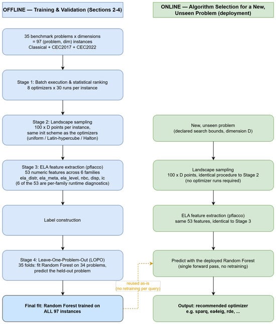
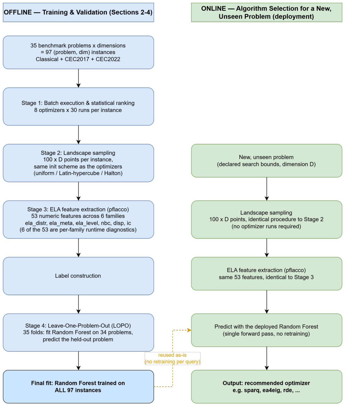
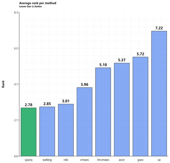
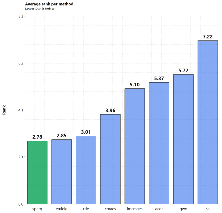
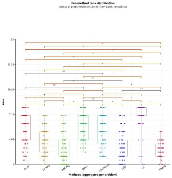
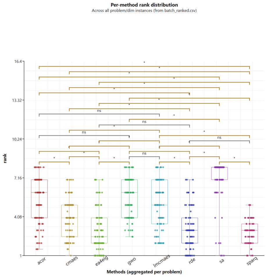

Disclaimer/Publisher’s Note: The statements, opinions and data contained in all publications are solely those of the individual author(s) and contributor(s) and not of MDPI and/or the editor(s). MDPI and/or the editor(s) disclaim responsibility for any injury to people or property resulting from any ideas, methods, instructions or products referred to in the content. |
© 2026 by the authors. Licensee MDPI, Basel, Switzerland. This article is an open access article distributed under the terms and conditions of the Creative Commons Attribution (CC BY) license.