


Abstract
Physics-informed anomaly detectors for industrial control systems are usually validated on a single synthetic or testbed dataset, which can yield optimistic estimates that do not transfer to deployment-like conditions. This validation-to-deployment discrepancy, the reality gap, is normally treated as one phenomenon and attributed to generic domain shift. We argue that it comprises at least three mechanistically distinct failure modes and propose a taxonomy that separates them by what a practitioner can observe and act on: Type 1, cross-regime evaluation; Type 2, operating-point shift; and Type 3, temporal distribution shift. A single physics-informed framework combining a Kalman-filter validation engine, BiLSTM, β-VAE, and graph attention network with residual sharing is evaluated across HAI 23.05, SWaT, and WADI over five random seeds. The three cases behave differently. Type 1 shows a substantial cross-regime decrease: AI-only falls from 0.774 in the prior synthetic evaluation to 0.493 on HAI, and Full EADE from 0.798 to 0.496. Under the retrospective fixed-FPR comparison on HAI, GNN+BiLSTM has the highest mean F1 at 0.498, although it is not separable from Full_EADE across five seeds. Type 2 collapses to FPR = 0.850 with F1 ≈ 0.237 across configurations; a strongly shifted sensor gives the clearest localized signature, but the failure is driven by aggregate distributional change and is recoverable by global threshold recalibration. Type 3 shows moderate FPR (0.244) and the largest sensitivity to residual occlusion (ΔF1_occl = +0.086), although a trained residual-free ablation shows no corresponding loss on any dataset. The resulting taxonomy links distinct failure signatures to different deployment responses.
1. Introduction
Anomaly detection in Industrial Control Systems (ICSs) has advanced rapidly through the integration of physics-based process models with data-driven machine learning, an approach broadly termed physics-informed anomaly detection [1,2]. Hybrid architectures that combine Physics Validation Engines (PVEs) with multi-model AI ensembles have demonstrated strong performance on synthetic and single-testbed benchmarks, achieving F1 scores above 0.79 with controlled false positive rates [3]. One problem, however, keeps these systems out of practical deployment. Models validated under a single dataset or operating regime can exhibit substantial performance changes when evaluated across datasets, installations, or temporally shifted operating conditions [4,5]. This validation-to-deployment discrepancy is commonly referred to as the reality gap.
The reality gap in ICS anomaly detection is typically treated as a single phenomenon, attributed to generic “domain shift” or “distribution mismatch” between training and test data [6,7]. Prior work addresses it through domain adaptation techniques, transfer learning, or more representative data generation, implicitly assuming that a single mitigation strategy suffices. We argue that this monolithic treatment hides real structure. The reality gap is not one problem but at least three mechanistically distinct failure modes, each with its own causal mechanism, diagnostic signature, and mitigation strategy.
The classical account of distribution shift is statistical: it classifies what has changed in the joint distribution. The taxonomy proposed here cuts the problem along a different axis, namely what a practitioner can observe during commissioning and what response that observation licenses. Section 2.3 sets this against the specific prior work it responds to. This paper proposes a three-type reality gap taxonomy for physics-informed ICS anomaly detection:
Type 1: Cross-Regime Evaluation Gap. The same detection framework, independently instantiated and trained in a synthetic regime and a real-testbed regime, exhibits a substantial performance discrepancy between the two evaluations. The F1 degradation is consistent with differences in process variability, attack repertoire and generator fidelity across the two regimes. These factors are confounded in the present comparison, so no single causal source is isolated. The FPR operating point is fixed by oracle construction and is not a deployment diagnostic. The degradation is diffuse across multiple sensors, with no single sensor dominating the effect.
Type 2: Operating-Point Shift Gap. A physical process parameter changes between the training period and the test period within the same installation. This produces a catastrophic false positive rate (FPR) collapse, where the detector flags normal operation as anomalous because its learned “normal” no longer matches the current operating point. Critically, the diagnostic signature can be dominated by a single sensor whose mean has shifted by many standard deviations. The operating-point change is then highly localized and detectable through sensor-level statistical monitoring.
Type 3: Temporal Distribution Shift Gap. Non-stationarity within the same installation causes progressive divergence between training and test distributions, even without an explicit operating-point change. This manifests as gradual degradation rather than catastrophic failure, with the Graph Neural Network (GNN) component particularly susceptible to correlation-structure overfitting on training-period correlations. Unlike Type 2, no single sensor dominates; the shift is distributed across the sensor network. In our experiments, Type 3 is the only case with substantial inference-time residual-occlusion sensitivity. A separately trained residual-free ablation shows no corresponding performance gain, so this sensitivity is interpreted as model dependence rather than as evidence that physics residuals improve detection.
We validate this taxonomy using a unified detection architecture, the Edge AI Detection Engine (EADE) from the PhySec-Edge framework [3], comprising a Kalman-filter PVE with Normalized Innovation Squared (NIS) scoring, a bidirectional LSTM (64 units per direction), a β-variational autoencoder (latent dimension 16), and a two-layer Graph Attention Network, all connected through a residual-sharing mechanism that feeds continuous PVE residuals as auxiliary inputs to the BiLSTM temporal detector. This detection framework is evaluated using the same training protocol on three public ICS benchmarks, each exemplifying one gap type. The instantiation adapts feature dimensionality and the PVE constraint graph to each dataset while keeping all hyperparameters and training procedures identical:
- HAI 23.05 [8,9] (Type 1): A hardware-in-the-loop testbed recording 86 variables (79 used after excluding 7 DCS logic features) with 14 attack scenarios in Test Set 1 (54,000 samples, 2981 attack samples), providing real process data against which the synthetic-regime benchmark is compared.
- SWaT [10,11] (Type 2): A water treatment testbed where the normal recording period (22–28 December 2015) and attack period (28 December–2 January 2016) exhibit a 10.94σ mean shift in AIT201 (NaCl concentration), creating a clean operating-point shift example.
- WADI [10,11] (Type 3): A water distribution testbed with a 14-calendar-day normal recording span (784,571 retained observations, approximately 9.1 days of sampled data) and a subsequent attack period exhibiting temporal non-stationarity confirmed by VAE early stopping at epoch 7 and GNN correlation-structure overfitting from epoch 2.
Table 1 summarizes the key findings across the three benchmarks. HAI represents a cross-regime evaluation (synthetic-regime benchmark vs. real-testbed evaluation), while SWaT and WADI represent within-dataset splits where the gap arises from temporal properties of the data itself, not from domain transfer. This distinction is deliberate: we select each dataset because it most cleanly isolates one gap type, not because all three constitute a single generalization benchmark.
Table 1.
Reality gap taxonomy: summary of findings across three ICS benchmarks. HAI uses cross-regime evaluation (synthetic-regime benchmark vs. real-testbed evaluation); SWaT and WADI use within-dataset temporal splits. F1 values are means across five random seeds (7, 13, 42, 99, 2024).
The contributions of this paper are threefold: (i) a mechanistic taxonomy of three reality gap types in ICS anomaly detection, with formal definitions based on FPR behavior, sensor localization, and dominant failure mechanism; (ii) empirical validation on three public benchmarks using the same detection framework and training protocol, instantiated with dataset-specific feature mappings and physics constraint graphs (HAI 23.05: 8 edges; SWaT: 14 edges; WADI: 6 edges), with reproducibility assessed across five random seeds; and (iii) analysis of when trained detectors depend most on physics-informed residual inputs, measured by inference-time occlusion: strongly under temporal shift (Type 3, ΔF1_occl = +0.086), and negligibly under cross-regime evaluation (Type 1, +0.004) and operating-point shift (Type 2, −0.001). A separately trained residual-free ablation shows no corresponding gain on any dataset, which establishes occlusion sensitivity as a diagnostic of model dependence rather than as evidence of a performance contribution. This gives practitioners deployment-relevant guidance.
HAI is included as the Type 1 reference case. An earlier analysis of this dataset within the same research line is reported in [12]. The SWaT and WADI analyses, and the three-type taxonomy itself, are new contributions of the present work. The remainder of this paper is organized as follows. Section 2 reviews related work on ICS anomaly detection, distribution shift, and benchmark usage. Section 3 describes the detection architecture, defines the three-type taxonomy formally, and specifies the evaluation protocol. Section 4 characterizes each dataset and its associated gap type. Section 5 presents experimental results across five random seeds. Section 6 discusses deployment implications and limitations. Section 7 concludes the paper.
2. Related Work
2.1. Physics-Informed Hybrid Anomaly Detection in ICS
Physics-informed anomaly detection combines first-principles process models with data-driven machine learning to exploit complementary detection strengths [1,2]. The PhySec-Edge framework [3] introduced a layered architecture integrating a Kalman-filter Physics Validation Engine (PVE) with a multi-model Edge AI Detection Engine (EADE). That work showed that continuous residual sharing between physics and AI layers produces stronger detection than either alone (ΔF1 = +0.017 on synthetic data). EvoPhySec [13] extended this with multi-objective evolutionary calibration using NSGA-III, achieving adaptive per-domain configuration. Graph neural network approaches for multivariate ICS time series exploit inter-sensor dependencies [14], while physics-constrained graph attention networks incorporate physical conservation relations directly into the detection architecture [15]. Recent hybrid studies and systematic reviews further emphasize the value of complementary detection mechanisms in CPS/ICS security [16,17]. Broader reviews of AI-enabled intrusion detection similarly identify adaptive and hybrid designs, realistic datasets, and real-world applicability as central requirements for deployable systems [18].
2.2. ICS Benchmarks and Their Usage
Three publicly available ICS testbed datasets dominate the anomaly detection literature: SWaT [10,11], WADI [10,11], and HAI [8,9]. SWaT provides a six-stage water treatment process with 51 sensor/actuator channels and 36 labeled attack scenarios. WADI extends this to a water distribution network with 123 channels and 15 attack scenarios. HAI provides a hardware-in-the-loop testbed combining a boiler, turbine, and water treatment loop with 86 channels, four training files, and two test sets containing 52 attack scenarios in total (14 in Test Set 1, 38 in Test Set 2). These datasets are commonly used as independent benchmarks, with models trained and tested within a single dataset and compared against methods evaluated under the same benchmark-specific setup [4,10,11,19]. Cross-domain evaluation remains relatively uncommon in ICS anomaly detection, although recent work has begun to investigate canonical feature alignment, domain-adversarial learning, and zero-shot transfer across heterogeneous industrial benchmarks [5]. However, existing studies primarily characterize transfer performance rather than systematically distinguishing the mechanisms and diagnostic signatures of different forms of deployment-related degradation.
2.3. Distribution Shift in Time Series Anomaly Detection
Distribution shift and concept drift are well-established problems in machine learning [20,21]. In industrial systems, related work typically addresses individual mechanisms, including operational-drift and operating-point change detection [22,23], iterative or incremental adaptation under concept drift [24], and cross-domain transfer or domain adaptation [5]. However, these approaches treat each mechanism in isolation. The classical taxonomy is statistical: it classifies what has changed in the joint distribution. Our three types cut the problem along a different axis, namely what a practitioner can observe and act on. Type 2 is a covariate shift, but a localized one whose mechanism, a change in process setpoint, is what makes threshold recalibration the appropriate response; the statistical label on its own does not separate it from sensor noise. Type 3 combines gradual covariate shift with a change in inter-sensor correlation structure, two changes that the classical scheme treats as a single phenomenon but that leave different diagnostic traces. Type 1 falls outside the classical scheme altogether, because training and test data originate in different generating regimes rather than in one distribution that has moved. We are not aware of prior work that formally distinguishes types of reality gap based on their causal mechanism, diagnostic signature, and optimal mitigation strategy. That is the contribution of this paper.
2.4. Reality Gap and Cross-Benchmark Generalization
The ICS anomaly detection literature predominantly evaluates detectors on individual benchmarks: a model is optimized for SWaT, its F1 is compared against prior SWaT results, and generalization is implicitly assumed. Cross-benchmark studies are rare, and when they exist, they typically report aggregate performance degradation without analyzing why the degradation occurs or whether it has the same character across datasets. A model that achieves F1 = 0.95 on SWaT and F1 = 0.60 on WADI may be experiencing operating-point mismatch, temporal drift, or architectural unsuitability, but the single-number comparison provides no diagnostic information.
This gap in evaluation methodology has practical consequences. A practitioner deploying an ICS anomaly detector cannot determine from published benchmarks whether poor cross-dataset performance indicates a fundamental architectural limitation (requiring a new model) or a calibration mismatch (requiring threshold adjustment). The monolithic “domain shift” framing provides no actionable guidance.
This work contributes a diagnostic framework for interpreting detector failure under deployment-like shifts, not a new detector architecture. We demonstrate that the same detection framework, applied under an identical training protocol to three datasets, exhibits three qualitatively different failure modes, and that these failure modes are distinguishable through observable deployment statistics. Type 2 and Type 3 can be screened using verified-normal commissioning data (FPR profile, per-sensor z-scores) without ground-truth attack labels; Type 1 requires a cross-regime performance assessment to establish the F1 degradation.
3. Methodology
3.1. Detection Architecture
We employ the PhySec-Edge EADE architecture [3] as a unified detection platform across all three datasets. The architecture comprises four components:
Physics Validation Engine (PVE). A Kalman-filter state estimator computes per-sensor residuals ri(t) = si(t) − ŝi(t) and Normalized Innovation Squared (NIS) scores. Cross-sensor consistency checks and gradient-bound validators generate a physics alert level α_P ∈ {0, 1, 2} (normal, soft anomaly, hard violation). Each constraint edge encodes a mass- or flow-conservation relation read from the published process schematic of the corresponding testbed, so the graphs are specified manually and are not learned from data. The PVE constraint graph is dataset-specific: 14 edges for SWaT (flow conservation across 6 stages), 6 edges for WADI (conservative sparse graph), and 8 edges for HAI (boiler–turbine–water coupling). PVE calibration uses a 5σ gradient bound and AR(1) process model with α = 0.99 exponential smoothing for near-constant sensors.
BiLSTM Temporal Detector. A bidirectional LSTM with 64 hidden units per direction processes sliding windows (W = 60 timesteps) over the augmented sensor stream [s(t); r(t)], where s(t) is the normalized sensor vector and r(t) ∈ ℝ8 is the PVE residual vector. All three datasets share the same eight-residual PVE structure (R1-R8); only the sensor count differs: 56 analog channels for HAI (64-dimensional BiLSTM input), 25 for SWaT (33-dimensional), and 44 PV channels for WADI (52-dimensional). The model is trained on normal-only sequences and scores test windows by hidden-state trajectory deviation. Sliding-window scores are assigned to each window’s final timestep (position i + W − 1 for window i), so no score depends on samples later than the timestep it is compared against.
β-Variational Autoencoder (β-VAE). A variational autoencoder with latent dimension 16 and β = 0.5 computes per-sensor reconstruction error on the normalized sensor vector s(t) (p1-p99 robust scaling). The VAE does not receive PVE residuals; residual sharing is implemented only in the BiLSTM input.
Graph Attention Network (GAT). A two-layer GAT with 4 attention heads encodes inter-sensor dependencies using the PVE constraint graph as topology. Node features are [z-score, VAE reconstruction error, temporal gradient], three features per sensor node. The GAT is particularly sensitive to changes in cross-sensor correlation structure.
Residual Sharing. The PVE residual vector r(t) ∈ ℝ8 is concatenated with the normalized sensor vector s(t) as input to the BiLSTM; the VAE and GNN do not receive residuals. All three datasets use the same eight PVE constraint groups (R1–R8); the BiLSTM input dimension is 56 + 8 = 64 for HAI, 25 + 8 = 33 for SWaT, and 44 + 8 = 52 for WADI. This converts the physics layer from a binary alert generator into a continuous signal amplifier. Weak anomalies that produce sub-threshold PVE deviations are still encoded in the residual vector and remain available to the BiLSTM temporal detector.
3.2. Evaluation Configurations
Four configurations isolate component contributions:
- GNN+BiLSTM: GAT process graph monitoring fused with BiLSTM temporal detection (no VAE, no PVE in decision).
- AI_only: VAE + GNN + BiLSTM ensemble (three AI components, no PVE score in decision).
- Full_EADE: All four components including PVE NIS score in the fusion decision.
- GNN+BiLSTM_ResidualOccluded: The trained GNN+BiLSTM model evaluated with the eight PVE residual channels replaced by a zero vector at inference time. This is an inference-time occlusion probe rather than an independently trained ablation: because the model was trained with residual channels present, occluding them at test time measures the sensitivity of the trained detector to residual availability. It does not isolate the causal training-time contribution of residual sharing, which would require training a separate model without residual channels under an identical protocol.
Residual sensitivity is quantified as ΔF1_occl = F1(GNN+BiLSTM) − F1 (GNN + BiLSTM_ResidualOccluded), using identical trained weights with and without residual information available at inference time. Throughout this paper ΔF1_occl is interpreted as a measure of how strongly the trained detector relies on residual inputs, not as the performance gain attributable to residual sharing during training. Section 5.3 reports a separately trained residual-free ablation that measures the latter directly.
3.3. Formal Definitions of the Reality Gap Taxonomy
We define three types of reality gap based on observable diagnostic signatures. Each definition specifies the causal mechanism, the FPR behavior (calibrated vs. collapsed), and the sensor localization pattern (diffuse vs. concentrated). Type 1 differs from the other two in the strength of evidence it can carry. Type 2 and Type 3 are controlled within-installation comparisons, using the same equipment and the same sensor set separated only in time. Type 1 compares two independently trained instances across different feature spaces and attack repertoires, so dataset scale, attack diversity, and generator fidelity are confounded with the regime change itself. Type 1 is therefore identified from a cross-regime performance comparison rather than from deployment statistics, and its diagnosis is correspondingly weaker. The fixed-FPR protocol equalizes the false-alarm budget among the HAI configurations; it does not place the synthetic and HAI evaluations at a matched operating point, since the synthetic baseline required for that comparison is not reproduced in the present study. Figure 1 summarizes the three types, the diagnostic signature associated with each, and the deployment response each implies.
Figure 1.
Three-type reality gap taxonomy for physics-informed ICS anomaly detection. Each type is characterized by its causal mechanism, FPR diagnostic signature, sensor localization pattern, dependence on residual inputs, and recommended deployment mitigation strategy.
Definition 1 (Type 1: Cross-Regime Evaluation Gap). A reality gap is Type 1 if the same detection framework is independently instantiated and evaluated in two different data regimes, R_A and R_B, each using its own training, calibration and evaluation data. No model weights are transferred between regimes. Regime R_A is, for example, a synthetic generator, and regime R_B a physical testbed. The two evaluations differ substantially in performance despite comparable evaluation objectives, such that the degradation is distributed across multiple sensors without a single dominant contributor. Because the regimes may differ in feature space, attack prevalence, attack repertoire and thresholding protocol, the cross-regime difference is read as evidence of degradation rather than as a prevalence-independent causal estimate. Matched operating-point evaluation should be used wherever the required baseline is available. Diagnostic signature: substantial cross-regime F1 degradation accompanied by diffuse sensor-level differences with no single dominant contributor. Recommended mitigation: improved source-regime fidelity or domain adaptation.
Definition 2 (Type 2: Operating-Point Shift Gap). A reality gap is Type 2 if it arises from a change in physical operating parameters between D_train and D_test within the same installation, such that: (a) FPR collapses catastrophically (FPR_test > 0.5); (b) a small number of sensors (typically 1–3) exhibit mean shifts exceeding 5σ relative to training statistics; (c) the shift originates in the data collection procedure rather than in model capacity, and the gap is recoverable by re-fitting the detection threshold on verified-normal data from the new operating point, without retraining. Diagnostic signature: FPR >> target, dominated by identifiable sensors. The localization signature identifies the gap type but not the remedy: Section 4.2 reports counterfactual tests in which correcting the dominant sensor fails while global threshold recalibration succeeds.
Definition 3 (Type 3: Temporal Distribution Shift Gap). A reality gap is Type 3 if it arises from non-stationarity within the same installation, where the training and test periods are drawn from temporally separated recordings of the same source without an explicit operating-point change, such that: (a) FPR is elevated but non-catastrophic (typically 2–10× the calibrated target, and FPR_test < 0.5); (b) distributional drift is diffuse across many sensors, with no single sensor exhibiting the extreme mean shift (>5σ) characteristic of Type 2; (c) drift is observable in marginal feature distributions and/or inter-sensor correlation structure across temporal partitions of the same recording. Diagnostic signature: Moderate FPR elevation (2–10× validation target), diffuse sensor degradation, and GNN training instability (validation loss divergence) as a secondary indicator. Expected detector behavior: increased instability of statistically learned representations and potentially stronger dependence on physics-informed inputs. Recommended mitigation: drift-aware recalibration or retraining, with adaptive relational structure evaluated where appropriate. Residual inputs may be retained for interpretability, but the present ablation does not support them as a performance-improving mitigation.
3.4. Evaluation Protocol
All primary experiments use five random seeds (7, 13, 42, 99, 2024), with results reported as mean ± standard deviation. Two threshold protocols are used. For HAI, the retrospective configuration comparison uses a fixed-FPR operating point: the threshold is set retrospectively to the 95th percentile of anomaly scores on verified-normal test samples, guaranteeing FPR = 5.0% by construction. For SWaT and WADI, thresholds are calibrated exclusively on normal validation data and then applied unchanged to the temporally separated test periods. Consequently, HAI FPR is fixed at 5.0% by construction, whereas SWaT and WADI FPR values reflect degradation of validation-calibrated thresholds under distributional shift. To confirm that the HAI classification does not depend on this choice, Section 5.6 also reports HAI under the validation-calibrated protocol used for SWaT and WADI. Metrics are F1-score, Precision, Recall, and FPR on the held-out test set. For SWaT and WADI, the temporal split follows the natural train/test boundary of the original datasets (normal period → train, attack period → test). For HAI, the model is trained on the HAI 23.05 normal training partition (files 1–2), validated on files 3–4, and evaluated on HAI 23.05 Test Set 1 (54,000 samples, 2981 attack samples, 5.52% attack rate, 14 attack scenarios). The synthetic PhySec-Edge results [3] serve as the prior-regime benchmark against which the HAI results are compared; no model weights are transferred between the two regimes.
Training hyperparameters are fixed across all datasets: VAE (50 epochs, batch 256, lr 1 × 10⁻³), BiLSTM (30 epochs, batch 512, window 60, lr 1 × 10⁻³), GNN (20 epochs, batch 256, lr 1 × 10⁻³), all with early stopping (patience 5, min_delta 1 × 10⁻⁴) and best-weights restoration.
4. Datasets and Gap Characterization
Table 2 summarizes the dataset characteristics and dominant gap mechanisms. We emphasize that we do not claim each dataset contains only one form of reality gap; rather, each dataset is selected because one gap mechanism is dominant and diagnostically observable. This gives a clean empirical exemplar for each type.
Table 2.
Dataset characteristics and dominant gap mechanisms. Features exclude label and timestamp columns. Attack rate computed on test/attack period only.
4.1. HAI 23.05: Type 1 Cross-Regime Evaluation Gap
The HIL-based Augmented ICS (HAI) 23.05 testbed [8,9] combines a boiler process, turbine process, and water treatment loop, recording 86 variables (56 analog sensors, 23 digital control signals, and 7 DCS logic variables excluded from detection input), yielding 79 features sampled at 1-s intervals. Test Set 1 contains 54,000 samples with 2981 attack samples (5.52% attack rate) spanning 14 distinct attack scenarios; the model is trained on the HAI normal partition (896,400 samples across training and validation files).
The PhySec-Edge proxy model [3] was trained and evaluated on a SWaT-inspired synthetic dataset (9875 samples, 7 attack types). The present work instantiates the same detection framework on HAI 23.05, training on the HAI normal partition and evaluating on HAI Test Set 1. Because the synthetic generator and the HAI testbed have different feature spaces, weight-level transfer is not feasible; the Type 1 gap is therefore measured as a cross-regime performance comparison between independently trained implementations from the same framework lineage. The mechanism remains a cross-regime one: the synthetic generator encodes simplified process dynamics, while the real HAI testbed exhibits higher variability, more complex transient behavior, and a richer attack repertoire.
The gap manifests as diffuse F1 degradation (0.798 → 0.498 for the highest-mean configuration), with FPR fixed at 5.0% by oracle construction. No single sensor dominates the degradation: residual magnitudes across the analog sensors are elevated but of comparable order, with no outlier of the kind seen for AIT201 on SWaT. For configurations available in both regimes, the conclusion holds consistently: AI-only degrades from 0.774 (synthetic) to 0.493 (HAI), and Full EADE from 0.798 to 0.496, so the cross-regime drop is not an artifact of comparing only the highest-mean configurations. This satisfies Definition 1 (Type 1): cross-regime comparison (synthetic benchmark vs. real testbed), oracle-fixed FPR, diffuse sensor-level degradation.
4.2. SWaT: Type 2 Operating-Point Shift
The Secure Water Treatment (SWaT) testbed [10,11] provides 51 features (25 sensors, 26 actuators) from a six-stage water treatment process. The normal period (495,000 samples, 22–28 December 2015) and attack period (449,919 samples, 28 December–2 January 2016, 36 attacks, 12.14% attack rate, 35 attack segments) are temporally contiguous but separated by a process restart.
A distribution shift analysis reveals that AIT201 (NaCl concentration in Stage 2, pre-treatment) exhibits a mean shift of 263.78 → 211.41 (z = 10.94σ) between the normal and attack recording periods, and the shift is present even in the non-attack segments of the attack file. All other sensors show shifts below z = 2.0. These shifts are measured on raw sensor readings, which is what a practitioner can inspect before any pipeline-specific preprocessing. The detector sees a smaller excursion: robust p1-p99 clipping against training percentiles maps the attack-period AIT201 mean from 211.41 up to 254.85, leaving a residual offset of 1.70σ at the model input. Clipping therefore absorbs most of the raw shift, and the FPR collapse survives it. This separation matters for how the 10.94σ figure should be read. It is what a practitioner sees in the raw data and is the diagnostic marker for Type 2, but it is not the magnitude the detector is exposed to, and the counterfactual tests below show that correcting the channel does not recover performance. The operating-point shift is most clearly signaled by AIT201, but the resulting threshold failure is system-level: the aggregate anomaly-score distribution moves beyond the validation-calibrated operating point, causing normal test segments to be classified as anomalous. The learned normal distribution did not include the attack-period AIT201 regime; however, the counterfactual tests below show that AIT201 is a diagnostic marker of the broader system-level operating-point shift rather than its sole causal bottleneck. Figure 2 shows the shift for every sensor.
Figure 2.
SWaT per-sensor mean shift between the normal and attack recording periods, measured in training-normalized standard deviations. AIT201 shifts by 10.94σ; the next-largest shift is 1.67σ, all other displayed sensors remain below 2σ, and the 15 sensors omitted from the figure fall below 0.33σ. Shifts are computed on the normal segments of the attack file, so they reflect a change in operating point rather than attack activity. The dashed line marks the z > 5σ criterion of Definition 2. The analysis covers the 25 analog sensor channels. Shifts are computed on raw sensor readings; robust p1-p99 clipping reduces the AIT201 excursion seen by the detector to 1.70σ.
This satisfies Definition 2 (Type 2): within-installation shift, catastrophic FPR (0.850), single-sensor dominance (AIT201 z = 10.94σ, all others z < 2). The gap is a property of the data collection procedure rather than a model limitation. The operating point changed between recording sessions.
We tested directly whether the gap can be recovered by acting on AIT201. Using the trained models without retraining, the test period was re-scored under two inference-time interventions across all five seeds: dropping AIT201 from the input and removing its PVE constraint edge, and remapping AIT201 onto the training distribution. Neither recovers the operating point. Dropping the sensor raises FPR from 0.850 to 1.000 in the three AI configurations, because the validation-calibrated threshold then separates nothing; Full EADE reaches FPR = 0.053 but only by collapsing detection with it (recall 0.037, F1 0.052). Remapping AIT201 leaves FPR between 0.835 and 0.964. Single-sensor dominance in the shift statistic is therefore a diagnostic marker that the operating point moved, not the causal bottleneck. The threshold is invalidated by the aggregate distributional change across the sensor network, in which AIT402, AIT501, AIT202, and AIT502 also participate, and recovering it would require recalibrating the threshold itself on normal data from the new operating point rather than correcting any individual channel.
A third intervention acts on the threshold rather than on the sensors. We re-fitted the detection threshold at the 95th percentile of anomaly scores computed on verified-normal data from the attack period itself, leaving inputs and weights unchanged. To avoid circularity the attack-period normal segments were split in half by time, the first half used for calibration and the second held out for measurement (197,619 and 197,620 samples). This changes the evaluation set, so the two conditions are compared only against each other on the held-out half, where attack prevalence is 21.7% rather than the 12.1% of the full test partition; F1 values from this comparison are not comparable with those in Table 3.
Table 3.
Detection results across five random seeds (7, 13, 42, 99, 2024). F1 and Precision are reported as mean ± std for all datasets. Recall is reported as mean ± std for HAI and as the mean across five random seeds for SWaT and WADI. FPR is averaged across the five random seeds for SWaT and WADI. HAI thresholds use a retrospective fixed-FPR protocol based on verified-normal test samples (FPR = 5.0% by construction), under the sliding-window alignment convention stated in Section 3.1. SWaT and WADI thresholds are calibrated on normal validation data; FPR values reflect threshold degradation under deployment-like conditions. The GNN+BiLSTM_ResidualOccluded configuration uses all five seeds.
Under the validation-calibrated threshold, every one of the 197,620 held-out normal samples is flagged as anomalous. Re-fitting the threshold on the new operating point reduces held-out FPR to 0.217 and raises F1 from 0.345 to 0.602 for GNN+BiLSTM (paired t(4) = 5.51, p = 0.005), with the same pattern in all four configurations. Recall falls from 0.962 to 0.731 while precision rises from 0.210 to 0.529: the detector stops flagging everything and begins to discriminate. The threshold required at the new operating point is 2.02 times the validation-calibrated one. Four of the five seeds fall below FPR = 0.5 on the held-out half; seed 99 reaches 0.514, so the recovery is substantial but not uniform across initializations. Taken together, the three interventions locate the Type 2 failure precisely. It is not attributable to any individual sensor, since correcting the dominant one changes nothing, but it is recoverable at the decision layer, since re-fitting a single scalar threshold on a window of verified-normal data restores most of the lost discrimination.
4.3. WADI: Type 3 Temporal Distribution Shift
The Water Distribution (WADI) testbed [10,11] provides 123 retained channels (after removing 4 permanently empty columns) from a water distribution network. Of these, 44 are process-value (PV) sensor channels and serve as detector inputs; the remainder are status, setpoint, and control-output channels. The normal period (784,571 samples, ~9 days) and attack period (172,803 samples, ~2 days, 5.77% attack rate, 15 attack scenarios) are from separate recording sessions in October 2017.
Three diagnostics provide evidence consistent with temporal non-stationarity rather than operating-point shift. First, VAE validation loss increases from epoch 2, and early stopping triggers at epoch 7. Even the last 20% of the normal training data therefore diverges from the first 80%. Second, GNN validation MSE explodes from 2.37 to 29+ immediately after epoch 1. Training-period correlation structure does not generalize even within the normal data. Third, several sensors exhibit systematic offsets (e.g., 2B_AIT_002_PV mean = 4427 with std = 4035; 3_AIT_004_PV min = −1770, max = 2780) requiring p1-p99 robust clipping to prevent loss explosion, but no single sensor shows the extreme z-score shift characteristic of Type 2. A direct distributional analysis of the 14-calendar-day normal recording span, comprising 784,571 retained one-second observations (~9.1 days of sampled data, split 50/50), confirms this pattern: 82 of the 123 retained channels (67%) show distributional drift by KS test (p < 0.05). The drift is most pervasive on the measurement side of the plant: all 44 process-value sensor channels drift significantly, compared with 38 of the 79 status, setpoint, and control-output channels; all 82 rejections survive Benjamini–Hochberg FDR correction (q < 0.05), as p-values are numerically indistinguishable from zero at n = 392,285 per half. Primary emphasis is therefore placed on KS effect sizes and mean shifts reported below. Drift concentrates in the analytical instrument transmitters: all 18 AIT channels drift significantly, and the AIT family has a mean KS statistic of 0.366 against 0.149 for the next-highest family, consistent with gradual water chemistry changes over the recording period (1_AIT_003_PV: KS = 0.855, mean shift = 1.73σ; 3_AIT_005_PV: KS = 0.756, 1.18σ; 2B_AIT_001_PV: KS = 0.559, 1.45σ; 2A_AIT_001_PV: KS = 0.578, 1.40σ). No channel exceeds a mean shift of 1.73σ and none approaches the z > 5σ threshold that characterizes Type 2, so the drift is diffuse rather than localized. The Frobenius distance between sensor correlation matrices of the two halves is 8.72 (33% of the first-half matrix norm). Inter-sensor correlation structure changes substantially over the recording period. Together, these data-level measurements provide evidence of temporal non-stationarity independent of model behavior. Figure 3 summarizes the per-channel drift statistics.
Figure 3.
WADI distributional drift across the 14-calendar-day normal recording span, measured as the two-sample Kolmogorov–Smirnov statistic between the first and second half of the normal data (392,285 samples per half). Left: all 123 process channels ranked by KS statistic, with analytical instrument transmitters (AIT) highlighted. Right: mean KS statistic by channel family, for families with at least three channels. Drift concentrates in the AIT family, but no single channel dominates: the largest mean shift is 1.73σ, well below the z > 5σ criterion for Type 2.
This satisfies Definition 3 (Type 3): within-installation non-stationarity, elevated but non-catastrophic FPR (0.244), distributed degradation, GNN particularly affected, with substantial inference-time residual-input dependence.
5. Results
5.1. Cross-Dataset Results Across Five Random Seeds
Table 3 summarizes the evaluated configurations across all three datasets and five random seeds.
Figure 4 illustrates these results visually. Three qualitatively different patterns emerge, each consistent with the predicted gap type:
Figure 4.
Detection performance (F1) and residual occlusion sensitivity across gap types. Bar groups show four detector configurations per dataset. ΔF1_occl annotations indicate the performance difference between GNN+BiLSTM evaluated with and without PVE residual inputs available at inference time, using identical trained weights. For HAI, both the plotted GNN+BiLSTM bar and the ΔF1_occl annotation are computed across all five seeds. Because HAI uses a retrospective fixed-FPR operating point whereas SWaT and WADI use validation-calibrated deployment thresholds, absolute F1 values should not be interpreted as a matched cross-dataset ranking.
HAI (Type 1): GNN+BiLSTM (0.498 ± 0.006), Full_EADE (0.496 ± 0.004) and AI_only (0.493 ± 0.004) span only 0.005 F1. GNN+BiLSTM and Full_EADE are not separable across the five seeds; both exceed AI_only consistently, but these configuration-level differences are small relative to the cross-regime degradation that defines Type 1. The residual PVE contribution is limited by NIS noise (standalone PVE FPR = 0.482 on HAI). Seed variance is low (std = 0.004–0.006 across the three main configurations), which indicates that the gap is a systematic property of the cross-regime evaluation rather than an initialization effect.
SWaT (Type 2): All configurations produce essentially identical F1 (≈0.237, range 0.237–0.238). The operating-point shift dominates detector behavior regardless of configuration, with AIT201 providing the strongest localized statistical signature. Recall is extremely high (0.943–0.975) because the models identify most attack samples, but they also flag most normal segments as anomalous (FPR = 0.827–0.863).
WADI (Type 3): Full_EADE achieves the best F1 (0.158 ± 0.019), followed by AI_only (0.149) and GNN+BiLSTM (0.131). This is the only dataset where the full physics-informed fusion outperforms the AI-only configuration. Complete PVE integration, including the NIS decision score, adds value under temporal distribution shift. The separate inference-time occlusion analysis (Section 5.3) further shows that the trained detector depends strongly on residual input availability. The higher variance (std = 0.019) reflects sensitivity to which seeds produce better GNN early-stopping points.
5.2. Seed Stability and Failure Consistency
The standard deviation across seeds provides a secondary diagnostic. For HAI (Type 1), the configurations share the same five seeds, so comparisons can be made pairwise, reducing the seed effect reflected in the marginal standard deviations. The low variance (std ≤ 0.006) indicates that the observed degradation is a systematic property of the cross-regime evaluation rather than an artifact of stochastic initialization. GNN+BiLSTM exceeds AI_only in all five seeds (mean difference +0.005), and Full_EADE exceeds AI_only in all five (+0.004). GNN+BiLSTM and Full_EADE are not separable: the mean difference is +0.002 and the sign is inconsistent across seeds. We report the paired Wilcoxon signed-rank test, which gives W = 0 and p = 0.063 for the two consistent comparisons. At n = 5 the smallest attainable two-sided p-value is 0.063, so the test cannot reach the conventional threshold however large the effect. We therefore read the consistent direction across all five seeds as evidence of stable ordering rather than as a decisive significance claim, and we do not claim an ordering between GNN+BiLSTM and Full_EADE at this sample size. The three configurations span 0.005 F1 in total, which is small against the cross-regime degradation the gap type describes.
For SWaT (Type 2), the near-identical F1 across all configurations and seeds (std = 0.002–0.004) confirms that architecture choice is not the limiting factor under operating-point shift. The operating-point shift dominates detector behavior regardless of model capacity or initialization, with AIT201 providing the strongest localized statistical signature. Paired comparisons across the shared seeds bear this out: GNN+BiLSTM and AI_only are indistinguishable (mean difference +0.0001; 3 of 5 seeds favor GNN+BiLSTM; W = 7, p = 1.00; t(4) = 0.10, p = 0.92), as are Full_EADE and GNN+BiLSTM (+0.0010; 3 of 5; W = 3, p = 0.31; t(4) = 1.53, p = 0.20). Full_EADE exceeds AI_only in all five seeds by +0.0011 (W = 0, p = 0.063; t(4) = 13.02, p = 0.0002). The direction there is perfectly consistent, but the difference of one thousandth of an F1 point is operationally meaningless. The large t-statistic reflects how small the between-seed variance is, not the importance of the effect, which is the clearest illustration in this study of why we do not read these comparisons from p-values alone.
For WADI (Type 3), the higher variance (std = 0.019 for Full_EADE) reflects sensitivity to temporal representation learning under non-stationary correlation structures. Seeds that produce GNN early-stopping at a more representative validation epoch achieve better test performance. This variance itself is a Type 3 signature: the learning dynamics are more fragile under temporal drift. The configuration ordering on WADI is nevertheless consistent across every seed. Full_EADE exceeds AI_only in all five seeds (mean difference +0.008; W = 0, p = 0.063; t(4) = 3.37, p = 0.028) and exceeds GNN+BiLSTM in all five (+0.026; W = 0, p = 0.063; t(4) = 4.27, p = 0.013), while AI_only exceeds GNN+BiLSTM in all five (+0.018; W = 0, p = 0.063; t(4) = 3.63, p = 0.022). As for the other two datasets, we treat the consistent direction across all five seeds as the primary evidence, since the Wilcoxon statistic cannot fall below 0.063 at this sample size. The occlusion effect is substantially larger than any of these configuration-level differences (+0.086, t(4) = +35.13, p = 0.000004; Wilcoxon W = 0, p = 0.063; positive in all five seeds). At n = 5 the smallest attainable two-sided Wilcoxon p-value is 0.063, so the test cannot reach conventional significance regardless of effect size; the consistent direction across all five seeds is the primary evidence.
5.3. Residual Contribution: Occlusion Compared with a Trained Ablation
Residual sharing feeds continuous PVE residuals as auxiliary inputs to the BiLSTM temporal detector. Table 4 quantifies how strongly each trained detector relies on those inputs by occluding the residual channels at inference time. A separately trained residual-free ablation, reported below, measures the complementary quantity: what the residual channels contribute while the model learns.
Table 4.
Inference-time residual occlusion analysis: ΔF1_occl = F1(GNN+BiLSTM) − F1(GNN+BiLSTM_ResidualOccluded). Identical trained weights; only the availability of the residual input channel differs at inference. Values quantify model sensitivity to residual inputs, not the training-time contribution of residual sharing.
The WADI result stands out (see also Figure 4, rightmost group). When residual inputs are occluded at inference, the trained GNN+BiLSTM detector drops from F1 = 0.131 to 0.045 (Recall = 0.044). The dependence on residual availability under the WADI evaluation is therefore strong. Both operating points nonetheless sit far below deployable accuracy, so the comparison establishes that the trained detector depends internally on residual inputs without establishing that residual sharing makes the detector usable on WADI. The WADI occlusion result therefore establishes strong dependence on residual availability at inference time, but does not by itself establish a training-time performance contribution. The separately trained residual-free ablation below tests that distinction directly. This does not establish that physics-based residuals are invariant to arbitrary distribution shifts, as the SWaT result shows that residuals can themselves be biased under operating-point change.
The SWaT result confirms the Type 2 prediction: when a localized sensor shift signals a broader operating-point mismatch, neither the AI components nor the physics residuals can compensate for a globally miscalibrated decision threshold.
Occlusion measures what a trained detector loses when an input is withdrawn. It does not measure what that input contributed while the model was learning. To separate the two, we trained GNN+BiLSTM from scratch without the eight PVE residual channels on all three datasets, using the same partitions, seeds, preprocessing, hyperparameters, early-stopping rule and threshold protocol as the main runs. The BiLSTM input dimension was reduced accordingly, from 64 to 56 on HAI, from 33 to 25 on SWaT, and from 52 to 44 on WADI.
The trained ablation does not reproduce the occlusion effect on any dataset. ΔF1_trained is 0.000 ± 0.005 on HAI, +0.006 ± 0.005 on SWaT and −0.017 ± 0.031 on WADI. None of the three differs significantly from zero across five seeds. The contrast with the occlusion values (+0.004, −0.001 and +0.086) is confined to WADI. On HAI and SWaT both measurements are near zero, so the two only diverge on the one dataset where occlusion sensitivity is substantial. The occlusion drop is therefore an input distribution shift rather than a loss of discriminative information. A model trained with eight residual channels degrades when those channels are replaced by zeros, but a model trained without them reaches equivalent performance. The BiLSTM learns a comparable representation from the sensor channels alone.
This result narrows the claim the taxonomy can support. Residual occlusion sensitivity remains a valid diagnostic signature and distinguishes Type 3 from Types 1 and 2, but it should not be read as evidence that physics residuals carry information the AI components cannot recover. Under the conditions tested here they do not. The practical consequence is that residual sharing cannot be justified on detection performance alone, and its value must rest on the interpretability of the physics layer or on behavior outside the three cases examined.
5.4. WADI Temporal Progression Analysis
To distinguish progressive temporal drift from a simple period-to-period difference, the WADI normal recording (784,571 samples) is divided into four equal chronological quarters (Q1–Q4, ≈196,143 samples each). For each subsequent quarter, two metrics are computed relative to Q1: the Frobenius distance between correlation matrices and the number of channels with significant distributional shift (two-sample KS test, Benjamini–Hochberg corrected, q < 0.05).
The Frobenius distance increases monotonically: 9.71 (Q1 → Q2), 10.53 (Q1 → Q3), 11.60 (Q1 → Q4), shown in Figure 5 (left). The inter-sensor correlation structure progressively diverges from the first quarter throughout the recording period. The number of significantly drifting channels remains persistently elevated at 78–83 of 123 across all quarter comparisons (Figure 5, right). The shift is stable rather than transient. The coarser first-half versus second-half comparison (Frobenius 8.72, 82 channels) understates the drift because it averages over the progression. Univariate KS statistics oscillate slightly (0.047 → 0.053 → 0.047), consistent with marginal distributions partially stabilizing while the inter-sensor correlation structure continues to diverge. This pattern is the expected signature of gradual water chemistry drift and distinguishes Type 3 from a step change.
Figure 5.
WADI temporal progression analysis. (A) Frobenius distance between the correlation matrix of Q1 and each subsequent quarter, showing monotonic increase (9.71 → 10.53 → 11.60). (B) Number of channels with significant distributional shift (BH-corrected KS test, q < 0.05) relative to Q1, persistently elevated at 78–83 of 123 across all quarters. Horizontal dashed lines show the coarser first-half versus second-half reference values. Each quarter contains ≈196,143 samples (≈2.3 days at 1 Hz).
5.5. Architecture Dependence of the Reality Gap: USAD Baseline
The results address the question of whether the observed gaps are a property of the data or of the detector architecture. USAD [4] uses a fundamentally different approach: two autoencoders with an adversarial training objective and no graph component, no physics engine, and no residual sharing. If a simpler architecture shows the same qualitative pattern across gap types, the gap is in the data. If it diverges, the architecture matters.
On HAI (Type 1), EADE leads USAD by 0.07–0.08 F1 at a matched oracle FPR of 5% (GNN+BiLSTM 0.498 vs. USAD 0.419), showing a clear performance advantage for EADE under the matched HAI operating conditions. On SWaT (Type 2), the gap between the two architectures collapses: EADE achieves 0.674 and USAD 0.665 under the same oracle threshold, a difference of 0.009 that is statistically significant across seeds (p < 0.001) but operationally negligible. Both architectures collapse to FPR > 0.83 under the validation-calibrated threshold. Under the retrospective oracle_fpr5 protocol of Table 5 both are then evaluated at FPR = 5% by construction, since that protocol sets the threshold from distribution of normal test samples and is not a recalibration procedure. Under the held-out evaluation of Section 4.2, where the recalibrated threshold is fitted on the first half of the attack-period normal segments and evaluated on the second half, held-out FPR falls to 0.217. The operating-point shift affects them identically because neither architecture can distinguish a threshold miscalibration from an attack.
Table 5.
EADE vs. USAD baseline at oracle FPR = 5% (retrospective threshold, five seeds, mean ± population std). USAD uses two autoencoders with adversarial training objective and no graph or physics component [4]. FPR is fixed at 5% by oracle construction and is shown as 0.050 for completeness.
Figure 6 shows the comparison across all three datasets. On WADI (Type 3), the two architectures diverge, but in the opposite direction: USAD (0.212) outperforms all EADE configurations (0.047 to 0.140), with a difference of 0.072 to 0.165 F1 (all p < 0.01). The mechanism is visible in the residual occlusion results. When residual inputs are occluded at inference, the trained GNN+BiLSTM detector drops from F1 = 0.131 to 0.045 on WADI (Table 4), while USAD (0.212) shows no such drop, having no explicit graph component and therefore being potentially less exposed to the specific correlation-structure drift that impairs the GNN-based configuration. The GNN learns inter-sensor correlation structure from the training period; when that structure drifts across 82 of 123 channels (Frobenius distance 8.72), the fixed relational structure plausibly contributes to the loss. Because EADE and USAD differ in several architectural components, the present comparison does not isolate the GNN as the sole causal source. This finding qualifies the general recommendation of physics-informed hybrid architectures: learned graph-based relational structure can become a liability when inter-sensor correlations drift. Residual inputs remain strongly relied upon by the WADI-trained detector (ΔF1_occl = +0.086). The architecture-specific sensitivity is more closely associated with the GNN’s learned relational structure than with residual availability itself. The appropriate design choice depends on which gap type is anticipated.
Figure 6.
EADE vs. USAD baseline at oracle FPR = 5% across the three benchmark datasets. Each group shows three EADE configurations and the USAD baseline; error bars indicate population standard deviation across five seeds. Annotations below each group give the gap type and the qualitative outcome. Numerical values and significance tests are given in Table 5 and Section 5.5.
5.6. FPR as a Diagnostic Signature
Figure 7 presents the diagnostic patterns associated with the three gap types. For Type 2 and Type 3, FPR or alarm-rate behavior during a verified-normal commissioning period provides a practical diagnostic without requiring labeled attack examples. Type 1, by contrast, requires a cross-regime performance assessment. Matched operating-point evaluation should be used wherever the required baseline is available; for the synthetic-to-HAI comparison it is not.
Figure 7.
FPR diagnostic signature by gap type. The three diagnostic patterns (oracle-fixed, elevated, and catastrophic) provide a practitioner-oriented diagnostic heuristic for identifying the dominant reality gap mechanism from observed false positive behavior. Representative FPR values correspond to the configurations reported in Table 1; configuration-specific ranges are given in Table 3.
Because the HAI threshold is fixed retrospectively, the FPR it produces cannot be compared directly with the validation-calibrated values obtained on SWaT and WADI. To establish that the Type 1 classification does not depend on the protocol, HAI was re-scored under the validation-calibrated rule used for the other two datasets, with the threshold set to the 95th percentile of anomaly scores on the normal validation partition and then applied unchanged to Test Set 1.
The classification is unchanged. Under the validation-calibrated protocol, HAI FPR falls between 0.014 and 0.030 across the four configurations, below rather than above the 5% target, and far from both the Type 2 collapse (0.850) and the Type 3 elevation (0.244). F1 is correspondingly higher than under the oracle threshold: 0.574 ± 0.018 for GNN+BiLSTM, 0.562 ± 0.012 for AI_only and 0.570 ± 0.009 for Full_EADE. HAI therefore satisfies the Type 1 signature under both protocols, and the oracle operating point is retained in the main tables because it equalizes the false-alarm budget across the HAI configurations, which is the comparison the Type 1 diagnosis requires.
Type 1 (HAI): FPR = 0.050 by oracle construction. Because the HAI operating point is fixed retrospectively at FPR = 5%, its FPR is not interpreted as a deployment diagnostic. Type 1 is instead identified through the cross-regime F1 reduction (0.798 → 0.498) and diffuse sensor-level degradation, with the false-alarm budget equalized among the HAI configurations.
Type 2 (SWaT): FPR = 0.850, a catastrophic collapse. The model flags 85.0% of normal test data as anomalous. This is an unambiguous signal that the operating point has shifted: a practitioner observing FPR > 0.5 should immediately investigate sensor-level mean shifts rather than retraining the model.
Type 3 (WADI): FPR = 0.244, elevated but not catastrophic. The model’s normal boundary has partially drifted but retains some discriminative power. This intermediate FPR profile distinguishes Type 3 from both Type 1 (oracle-fixed) and Type 2 (collapsed), and provides a useful secondary indicator when combined with evaluation context and sensor-localization evidence.
The FPR ratio thresholds above (>0.5 absolute for Type 2; 2–10× for Type 3) apply to Type 2 and Type 3. Type 1 is not identified from an FPR zone because its HAI operating point is fixed retrospectively; it is identified through substantial cross-regime F1 degradation under an equalized false-alarm budget across the HAI configurations, combined with diffuse sensor-level evidence. The boundaries quoted here should be re-estimated for each installation from the variability of its own commissioning period rather than transferred as fixed constants, since the width of normal FPR fluctuation depends on process dynamics and sampling rate. The thresholds are heuristic zones derived from the three datasets studied and should be treated as practical starting points, not universal constants. The primary classification criterion is the data split type (cross-regime source vs. same-installation temporal split) and the sensor localization pattern; the FPR ratio is a supporting indicator for Type 2 and Type 3. This three-way FPR profile (oracle-fixed/catastrophic/elevated) constitutes a supporting diagnostic indicator; Type 1 is primarily identified through cross-regime F1 degradation and sensor-level evidence rather than FPR. The full guide is summarized in Table 6.
Table 6.
Gap-type diagnostic guide for deployment practitioners.
The separation between Type 2 and Type 3 is more evident in FPR space than in F1 space. This has a practical implication: FPR can be estimated on a reference normal or commissioning period without requiring labeled attack examples, so it stays usable as a diagnostic during initial system rollout.
6. Discussion
6.1. Why Dependence on Residual Inputs Differs Between WADI and SWaT
The USAD baseline comparison (Section 5.5) supports this interpretation: USAD, which has no graph component, outperforms all EADE configurations on WADI, a result consistent with the interpretation that architectures without a graph-based relational module are less exposed to the observed correlation drift. The asymmetry in dependence on residual inputs (ΔF1_occl = +0.086 for WADI versus −0.001 for SWaT) suggests that the WADI-trained detector relies substantially more on physics-informed inputs. Under temporal distribution shift (Type 3), the statistical patterns learned by the AI components (correlation structure, reconstruction baseline, temporal dynamics) gradually become stale. However, the PVE residuals are computed from first-principles physics models (conservation laws, constraint graphs) that do not depend on statistical learning and may therefore be less sensitive than purely learned representations to some forms of statistical drift. The residual channels provide a physics-grounded representation to which the trained WADI detector becomes strongly sensitive. The trained residual-free ablation shows that this dependence does not translate into a measurable performance contribution under the tested protocol.
As visible in Figure 4 (middle group, nearly identical bars), under operating-point shift (Type 2) both the physics model and the AI model are equally miscalibrated: the Kalman filter’s process model predicts AIT201 ≈ 264 (the training mean), just as the AI components expect AIT201 ≈ 264. Both systems generate large residuals/anomaly scores for the actual operating value of AIT201 ≈ 211. Residual sharing cannot help because the residuals themselves are systematically biased by the shift. They encode the operating-point mismatch, not the attack signal.
The two testbeds also share a physical origin for their drift, which strengthens the case that the two gap types are distinct rather than arbitrary. In both, the analytical instrument transmitters are the channels that move. On SWaT, nine of the ten most shifted sensors are AIT channels; on WADI, all 18 AIT channels drift significantly, with a family mean KS statistic of 0.366 against 0.149 for the next-highest family. Water chemistry therefore drifts in both installations. What separates Type 2 from Type 3 is not the physical cause but its concentration: on SWaT a single chemistry channel moves by 10.94σ while every other sensor stays below 2σ, whereas on WADI the movement is spread across the whole AIT family with no channel exceeding 1.73σ. The same underlying process produces a localized failure in one plant and a diffuse one in the other.
Type 3 exhibits the largest inference-time sensitivity to residual occlusion, but the separately trained residual-free ablation shows no corresponding performance loss. Residual occlusion is therefore useful here as a diagnostic of model dependence, not as evidence that residual sharing improves detection performance. The deployment rule that follows is about where to look rather than what to install: occlusion sensitivity distinguishes the Type 3 case from Types 1 and 2, and operating-point monitoring with global threshold recalibration remains the first response for installations with variable process setpoints.
6.2. Deployment Implications by Gap Type
Each gap type implies a different mitigation strategy:
Type 1 (Cross-Regime Evaluation): Improve the synthetic data generator to capture higher process variability, or apply domain adaptation techniques, for example fine-tuning on a small amount of target-domain normal data. Residual sharing does not offer a route here: the trained ablation in Section 5.3 finds ΔF1_trained = 0.000 ± 0.005 on HAI, so the residual channels contribute nothing measurable during training under the present protocol.
Type 2 (Operating-Point Shift): Implement online operating-point monitoring. In practice this means tracking per-sensor mean and variance statistics over rolling windows and triggering recalibration when any sensor exceeds a z-score threshold (e.g., z > 5σ relative to training statistics). The counterfactual tests in Section 4.2 show that the recalibration must act on the detection threshold as a whole: correcting the individual sensor that triggered the alarm leaves FPR essentially unchanged, whereas re-fitting the threshold on a verified-normal window at the new operating point cuts held-out FPR from 1.000 to 0.217. On SWaT the threshold needed at the new operating point was twice the training-calibrated value, so the monitoring loop should re-estimate the threshold itself rather than only rescale the offending channel. The EvoPhySec framework [13] provides a mechanism for automated recalibration through multi-objective evolutionary optimization. The WADI temporal-progression analysis in Section 5.4 suggests when to invoke it. The Frobenius distance between the correlation matrix of the calibration window and that of the current window grew from 9.71 to 11.60 across four chronological quarters spanning 9.1 days of sampled data. That quantity is computable online without labels, so it supports a trigger rather than a schedule: evaluate it at a regular cadence, daily for instance, and recalibrate after a sustained departure from the commissioning baseline. Under WADI-like dynamics this implies re-assessment on a weekly scale, but the appropriate interval depends on how fast a given installation drifts and should be established per site. Operating-point-aware recalibration should be attempted as the first response and can avoid the need for full model retraining, as the SWaT threshold-recalibration experiment in Section 4.2 demonstrates.
Type 3 (Temporal Distribution Shift): Prioritize drift-aware recalibration, periodic model refresh, and evaluation of adaptive relational structure. Residual inputs may be retained for interpretability, but the trained ablation in Section 5.3 does not support them as a performance-improving mitigation. The WADI occlusion result (F1 falls from 0.131 to 0.045 when residual channels are zeroed) measures how far the trained model has come to depend on those channels, not what they contribute. For long-duration deployments, periodic model refresh with recent normal data may further reduce the gap and should be evaluated in long-duration deployments.
6.3. Practitioner Diagnostic Guide
We propose a two-step diagnostic procedure (illustrated in Figure 7) for identifying the gap type in deployment:
Step 1: Observe the alarm rate on a verified-normal commissioning period (e.g., the first week of deployment, if labeled as attack-free by plant operators). Note: true FPR requires known-normal samples; in the absence of labels, alarm rate on presumed-normal data is used as a proxy. If FPR > 0.5, suspect Type 2 (operating-point shift). If FPR is 2–10× the calibrated target, suspect Type 3 (temporal drift). If neither pattern applies, FPR alone is insufficient to identify Type 1; a cross-regime performance assessment is required.
Step 2: For suspected Type 2, compute per-sensor z-scores. Calculate the mean shift of each sensor relative to training statistics. If one or few sensors exhibit z > 5σ, confirm Type 2 and re-estimate the global detection threshold on verified-normal data from the new operating point; correcting individual shifted channels alone may be insufficient. If the shifts are diffuse and FPR is elevated but not catastrophic, consider Type 3; otherwise investigate other shift mechanisms.
6.4. Implications for Benchmark Reporting
The findings of this study suggest that current ICS anomaly detection benchmark reporting practices are insufficient to characterize detector performance under realistic deployment conditions. We propose four reporting recommendations:
First, studies should always report FPR on normal segments of the test set, not only on attack segments. The SWaT result demonstrates that a detector with Recall = 0.962 and F1 = 0.237 may appear to detect nearly all attacks, but only because it flags 85.0% of normal test samples as anomalous. Without FPR, this result could be mistaken for strong detection rather than calibration failure.
Second, per-sensor distribution shift statistics (mean shift in training-normalized z-scores) should be reported for any within-dataset evaluation where the training and test periods are temporally separated. The SWaT AIT201 z = 10.94σ shift is not a model failure. It is a data property that would affect any threshold-based detector. Reporting this statistic prevents misleading comparisons between methods that happen to be more or less sensitive to the shifted sensor.
Third, studies should explicitly characterize their evaluation split as cross-regime (training and test from different synthetic or operational regimes), within-dataset temporal (training and test from different time periods of the same source), or within-dataset random (random train/test split of the same recording). These three split types produce fundamentally different gap mechanisms, and results are not comparable across split types.
Fourth, when reporting benchmark results on datasets with known non-stationarity (such as WADI), studies should report the early-stopping epoch and validation loss trend, as these provide evidence of whether the model’s learned representations generalize within the dataset.
6.5. Limitations
The FPR-based diagnostic thresholds proposed in Table 6 (e.g., FPR > 0.5 for Type 2, 2–10× validation FPR for Type 3) should be interpreted as practical heuristics derived from the three datasets studied, not as universal constants. Different industrial systems may require adjusted thresholds depending on process variability, sampling rate, and acceptable alarm burden.
A further limitation concerns the residual-sharing analysis. The GNN+BiLSTM_ResidualOccluded configuration reuses the weights of a model trained with residual channels present, so occluding those channels at inference introduces an input distribution shift of its own. The reported ΔF1_occl values therefore measure how strongly each trained detector depends on residual inputs and should not be read as the performance gain attributable to residual sharing during training. That controlled ablation is reported in Section 5.3. Trained residual-free models show no measurable loss on any of the three datasets, which places the occlusion effect in input distribution rather than information content and limits what the residual-sharing mechanism can be claimed to contribute. Several limitations constrain the generalizability of the proposed taxonomy. First, three datasets, while spanning different ICS domains (water treatment, water distribution, hardware-in-the-loop), do not exhaustively sample all possible gap types. Additional types may exist in other industrial contexts (e.g., chemical processing, power grid, manufacturing). Second, the taxonomy is developed primarily using a single physics-informed architecture, with USAD included as a secondary architecture-dependence check. Broader validation across additional detector families is therefore still required. Third, SWaT and WADI represent within-dataset temporal splits, not independent installations, so the taxonomy’s applicability to truly multi-site deployments requires further validation. Fourth, the PVE constraint graph is read from the process schematic of each testbed rather than learned, which limits scalability to installations without documented topology and makes the graph unresponsive to the correlation drift measured in Section 5.4. Finally, the present validation treats the three gap types as dominant exemplars and does not evaluate mixtures of mechanisms. The taxonomy should not be read as requiring mutual exclusivity. A deployment may exhibit more than one signature at once, and the behavior of such mixed cases remains to be validated.
7. Conclusions
This paper has proposed a three-type taxonomy for the reality gap in physics-informed ICS anomaly detection, distinguishing cross-regime evaluation gap (Type 1), operating-point shift (Type 2), and temporal distribution shift (Type 3). Each type exhibits a distinct diagnostic signature (Figure 1, Figure 2, Figure 3, Figure 4, Figure 5, Figure 6 and Figure 7): cross-regime F1 degradation with diffuse sensor-level differences, catastrophic FPR collapse, and elevated but manageable FPR, respectively. Each also calls for a different mitigation strategy.
Empirical validation on three public ICS benchmarks (HAI 23.05, SWaT, WADI) using a unified physics-informed architecture supports the proposed distinction: the three representative cases produce qualitatively different detection behaviors that cannot be collapsed into a single “domain shift” explanation. Sensitivity to residual occlusion differs across gap types, distinguishing the Type 3 case from Types 1 and 2: it is strongest under temporal drift (Type 3, ΔF1_occl = +0.086) and negligible under cross-regime evaluation (Type 1, +0.004) and operating-point shift (Type 2, −0.001). A trained residual-free ablation shows no corresponding performance gain, so this pattern is a diagnostic signature of how each detector has come to use its inputs rather than a measure of what physics residuals contribute.
For practitioners, the evaluation context, alarm-rate behavior, and sensor-localization pattern jointly indicate the dominant gap type, which in turn prescribes the mitigation: cross-regime adaptation or richer synthetic generation for Type 1, global threshold recalibration against the new operating point for Type 2, and drift-aware recalibration with periodic model refresh for Type 3. Treated this way, the reality gap becomes a classifiable engineering problem rather than a single undifferentiated obstacle.
Future work will extend the taxonomy along four directions: (i) validation on additional ICS domains (chemical processing, power grid) to identify potential additional gap types; (ii) development of automated gap-type classifiers that can diagnose the gap type in real time from deployment data statistics; (iii) integration with the EvoPhySec evolutionary calibration framework [13] to provide type-specific automated mitigation; and (iv) constraint graphs that are inferred from data and updated during deployment. The WADI result motivates the last of these directly. A GNN trained over a fixed constraint topology can learn relational representations tied to correlations that later drift, and the USAD comparison in Section 5.5 shows that an architecture carrying no such graph is less exposed to that drift.
Author Contributions
Conceptualization, D.R.; methodology, D.R.; software, D.R., A.E., I.M., M.S. and A.S.C.; validation, D.R., A.E., I.M., P.K., M.S. and A.S.C.; formal analysis, D.R.; investigation, D.R., A.E., M.S., P.K. and I.M.; data curation, A.E., P.K., A.S.C. and I.M.; writing—original draft preparation, D.R.; writing—review and editing, D.R., A.E., P.K., I.M., M.S. and A.S.C.; visualization, A.E., M.S., P.K. and I.M.; supervision, D.R.; project administration, D.R. All authors have read and agreed to the published version of the manuscript.
Funding
This research received no external funding.
Institutional Review Board Statement
Not applicable.
Informed Consent Statement
Not applicable.
Data Availability Statement
The HAI 23.05 dataset is publicly available at the repository cited in this manuscript. The SWaT and WADI datasets were obtained from their official providers and are subject to their respective access conditions. Experiment code, processed evaluation outputs, and trained model configurations are available from the corresponding author upon reasonable request.
Conflicts of Interest
The authors declare no conflicts of interest.
Abbreviations
The following abbreviations are used in this manuscript:
| BiLSTM | Bidirectional Long Short-Term Memory |
| EADE | Edge AI Detection Engine |
| FDR | False Discovery Rate |
| FPR | False Positive Rate |
| GAT | Graph Attention Network |
| GNN | Graph Neural Network |
| HAI | HIL-based Augmented ICS Security Dataset |
| HIL | Hardware-in-the-Loop |
| ICS | Industrial Control System |
| KS | Kolmogorov–Smirnov |
| NIS | Normalized Innovation Squared |
| PVE | Physics Validation Engine |
| SWaT | Secure Water Treatment |
| VAE | Variational Autoencoder |
| WADI | Water Distribution Testbed |
| β-VAE | Beta-Variational Autoencoder |
References
- Karniadakis, G.E.; Kevrekidis, I.G.; Lu, L.; Perdikaris, P.; Wang, S.; Yang, L. Physics-Informed Machine Learning. Nat. Rev. Phys. 2021, 3, 422–440. [Google Scholar] [CrossRef] [Scilit]
- Giraldo, J.; Urbina, D.; Cardenas, A.; Valente, J.; Faisal, M.; Ruths, J.; Tippenhauer, N.O.; Sandberg, H.; Candell, R. A Survey of Physics-Based Attack Detection in Cyber-Physical Systems. ACM Comput. Surv. 2018, 51, 76. [Google Scholar] [CrossRef] [Scilit] [PubMed]
- Radovanovic, D.; Savanovic, N.; Kresoja, P.; Janackovic, J.; Petrovic, T. PhySec-Edge: A Hybrid Physics-Informed and Edge AI Framework for Anomaly Detection in Industrial IoT Sensor Networks. J. Sens. Actuator Netw. 2026, 15, 58. [Google Scholar] [CrossRef] [Scilit]
- Kim, B.; Alawami, M.A.; Kim, E.; Oh, S.; Park, J.; Kim, H. A Comparative Study of Time Series Anomaly Detection Models for Industrial Control Systems. Sensors 2023, 23, 1310. [Google Scholar] [CrossRef] [Scilit] [PubMed]
- Akinsowon, T.; Jinad, R.; Rasheed, A.; Varol, C.; Baza, M.; Alshehri, A. Zero-Shot Cross-Domain Anomaly Detection for Water ICS: A PLC-Based Dataset and Transfer Learning Evaluation Across Heterogeneous Benchmarks. Appl. Sci. 2026, 16, 8005. [Google Scholar] [CrossRef] [Scilit]
- Garg, A.; Zhang, W.; Samaran, J.; Savitha, R.; Foo, C.-S. An Evaluation of Anomaly Detection and Diagnosis in Multivariate Time Series. IEEE Trans. Neural Netw. Learn. Syst. 2022, 33, 2508–2517. [Google Scholar] [CrossRef] [Scilit] [PubMed]
- Wu, Y.; Sicard, B.; Gadsden, S.A. Physics-Informed Machine Learning: A Comprehensive Review on Applications in Anomaly Detection and Condition Monitoring. Expert Syst. Appl. 2024, 255, 124678. [Google Scholar] [CrossRef] [Scilit]
- Shin, H.-K.; Lee, W.; Choi, S.; Yun, J.-H.; Min, B.-G. HAI Security Datasets. GitHub. 2023. Available online: https://github.com/icsdataset/hai (accessed on 1 August 2026).
- Chahine, K.; Noura, H.N. Features over Architecture: Physics-Informed Anomaly Detection in Industrial Control Systems. Future Internet 2026, 18, 308. [Google Scholar] [CrossRef] [Scilit]
- Fährmann, D.; Damer, N.; Kirchbuchner, F.; Kuijper, A. Lightweight Long Short-Term Memory Variational Auto-Encoder for Multivariate Time Series Anomaly Detection in Industrial Control Systems. Sensors 2022, 22, 2886. [Google Scholar] [CrossRef] [Scilit] [PubMed]
- Gulzar, Q.; Mustafa, K. Interdisciplinary Framework for Cyber-Attacks and Anomaly Detection in Industrial Control Systems Using Deep Learning. Sci. Rep. 2025, 15, 26575. [Google Scholar] [CrossRef] [Scilit] [PubMed]
- Radovanovic, D.; Markovic, D.; Kresoja, P.; Cvetkovic, A.S.; Radojcic, V.; Sarac, M.; Savanovic, N. Reality Gap Analysis in Physics-Informed ICS Anomaly Detection: From Synthetic Validation to HAI 23.05 Real-World Testbed Evaluation. Mach. Learn. Knowl. Extr. 2026, 8, 276. [Google Scholar] [CrossRef] [Scilit]
- Radovanovic, D.; Savanovic, N.; Janackovic, J.; Kresoja, P.; Papaz, B. EvoPhySec: A Multi-Objective Evolutionary Framework for Adaptive Calibration of Physics-Informed Anomaly Detection in Smart City IoT Networks. Big Data Cogn. Comput. 2026, 10, 285. [Google Scholar] [CrossRef] [Scilit]
- Zhang, D.; Wang, M.; Bu, Y.; Yu, J.; Yang, L. PdGAT-ID: An Intrusion Detection Method for Industrial Control Systems Based on Periodic Extraction and Spatiotemporal Graph Attention. Comput. Secur. 2025, 149, 104210. [Google Scholar] [CrossRef] [Scilit]
- Homaei, M.; Khazrak, I.; Molano, R.; Caro, A.; Avila, M. Graph Attention Networks with Physical Constraints for Anomaly Detection. ICT Express 2026, in press. [Google Scholar] [CrossRef] [Scilit]
- Jeffrey, N.; Tan, Q.; Villar, J.R. A Hybrid Methodology for Anomaly Detection in Cyber–Physical Systems. Neurocomputing 2024, 568, 127068. [Google Scholar] [CrossRef] [Scilit]
- Seo, J.K.; Lee, J.; Kim, B.; Shim, W.; Seo, J.T. AI-Based Anomaly Detection in Industrial Control and Cyber–Physical Systems: A Data-Type-Oriented Systematic Review. Electronics 2026, 15, 20. [Google Scholar] [CrossRef] [Scilit]
- Villafranca, A.; Thant, K.M.; Tasic, I.; Cano, M.-D. AI-Enabled IoT Intrusion Detection: Unified Conceptual Framework and Research Roadmap. Mach. Learn. Knowl. Extr. 2025, 7, 115. [Google Scholar] [CrossRef] [Scilit]
- Taormina, R.; Galelli, S.; Tippenhauer, N.O.; Salomons, E.; Ostfeld, A.; Eliades, D.G.; Aghashahi, M.; Sundararajan, R.; Pourahmadi, M.; Banks, M.K.; et al. Battle of the Attack Detection Algorithms: Disclosing Cyber Attacks on Water Distribution Networks. J. Water Resour. Plan. Manag. 2018, 144, 04018048. [Google Scholar] [CrossRef] [Scilit]
- Ben-David, S.; Blitzer, J.; Crammer, K.; Kulesza, A.; Pereira, F.; Vaughan, J.W. A Theory of Learning from Different Domains. Mach. Learn. 2010, 79, 151–175. [Google Scholar] [CrossRef] [Scilit]
- Lu, J.; Liu, A.; Dong, F.; Gu, F.; Gama, J.; Zhang, G. Learning under Concept Drift: A Review. IEEE Trans. Knowl. Data Eng. 2019, 31, 2346–2363. [Google Scholar] [CrossRef] [Scilit]
- Raman, M.R.G.; Ahmed, C.M.; Mathur, A. Machine Learning for Intrusion Detection in Industrial Control Systems: Challenges and Lessons from Experimental Evaluation. Cybersecurity 2021, 4, 27. [Google Scholar] [CrossRef] [Scilit]
- Flórez, A.; Rodríguez-Moreno, I.; Artetxe, A.; García Olaizola, I.; Sierra, B. CatSight, a Direct Path to Proper Multi-Variate Time Series Change Detection: Perceiving a Concept Drift Through Common Spatial Pattern. Int. J. Mach. Learn. Cybern. 2023, 14, 2925–2944. [Google Scholar] [CrossRef] [Scilit]
- Abdoune, F.; Nouiri, M.; Cardin, O. Digital Twin-Based Anomaly Detection under Concept Drift: A Comparison between Iterative Batch Learning and Incremental Learning Approaches. Expert Syst. Appl. 2026, 299, 130062. [Google Scholar] [CrossRef] [Scilit]
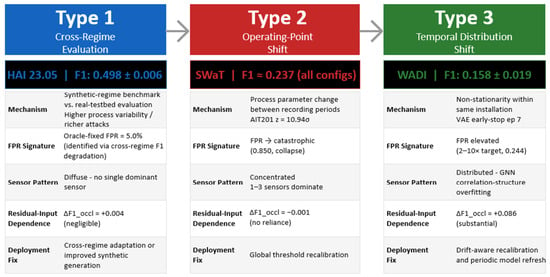
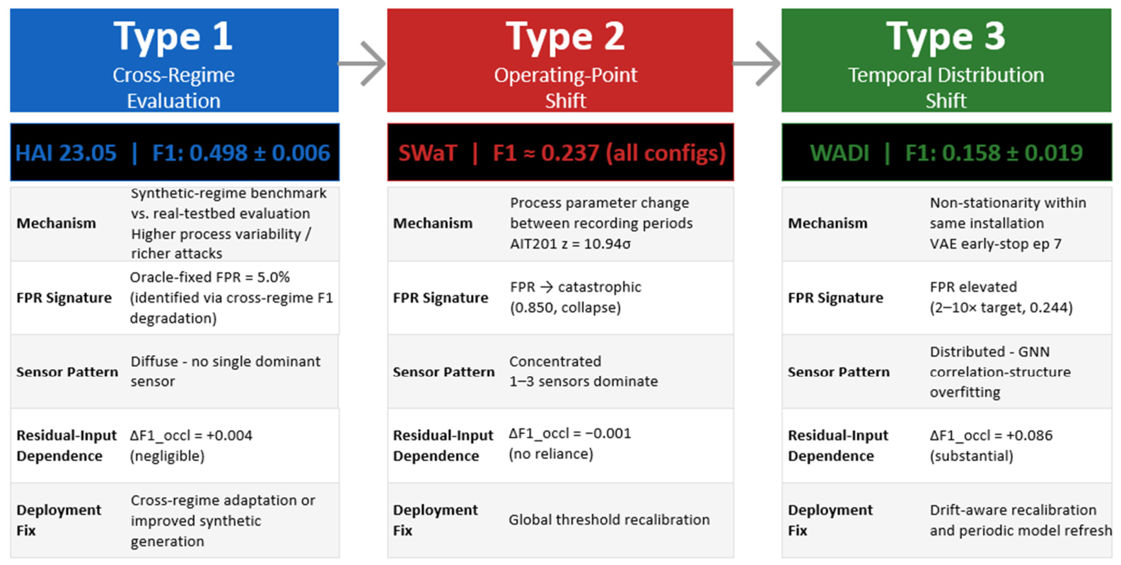
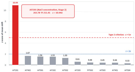
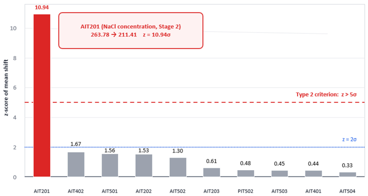
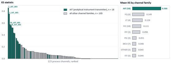
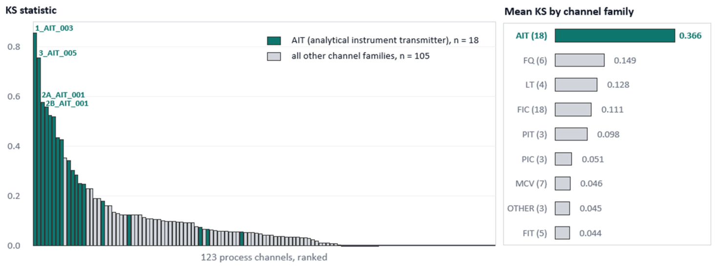
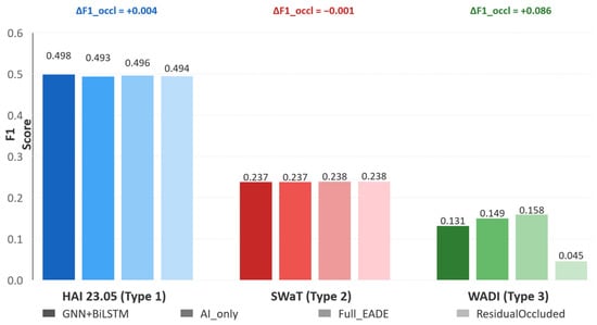
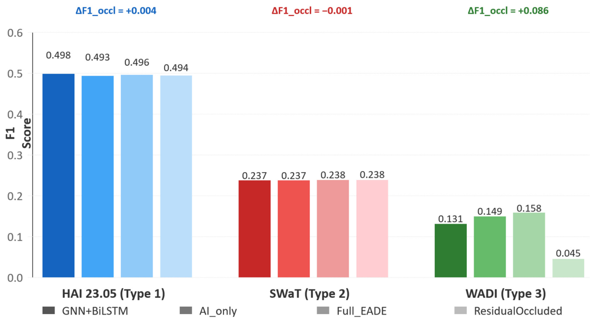
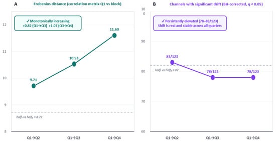
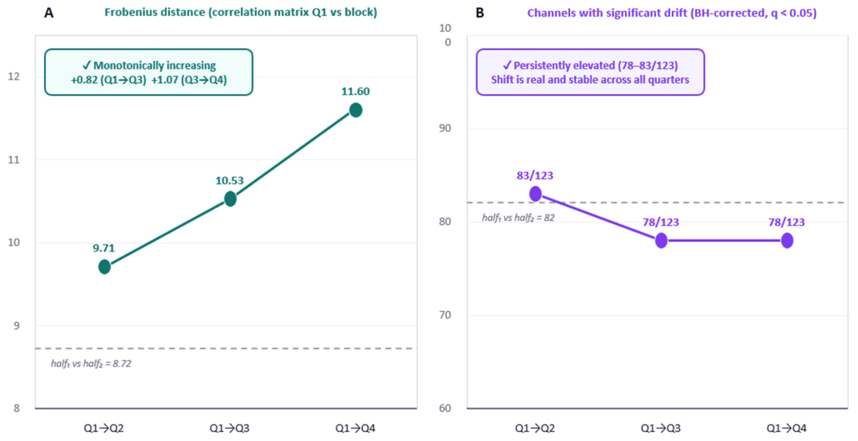
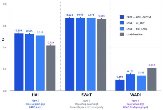
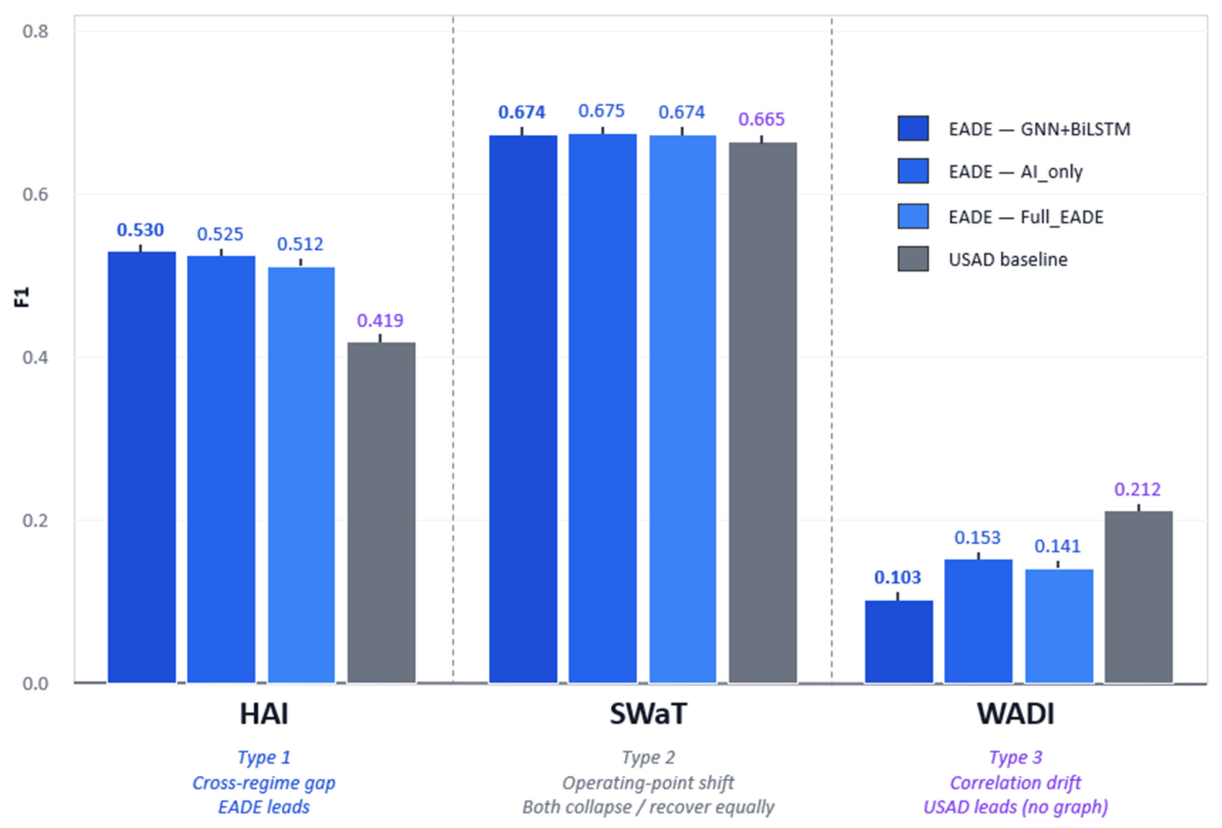
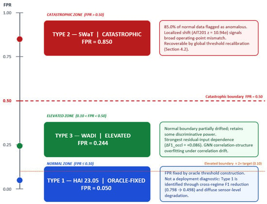
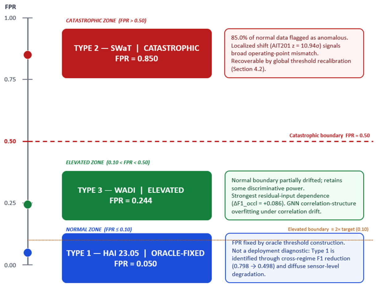

Disclaimer/Publisher’s Note: The statements, opinions and data contained in all publications are solely those of the individual author(s) and contributor(s) and not of MDPI and/or the editor(s). MDPI and/or the editor(s) disclaim responsibility for any injury to people or property resulting from any ideas, methods, instructions or products referred to in the content. |
© 2026 by the authors. Licensee MDPI, Basel, Switzerland. This article is an open access article distributed under the terms and conditions of the Creative Commons Attribution (CC BY) license.