Tabular Machine Learning Methods for Predicting Gas Turbine Emissions

Abstract

Predicting emissions for gas turbines is critical for monitoring harmful pollutants being released into the atmosphere. In this study, we evaluate the performance of machine learning models for predicting emissions for gas turbines. We compared an existing predictive emissions model, a first-principles-based Chemical Kinetics model, against two machine learning models we developed based on the Self-Attention and Intersample Attention Transformer (SAINT) and eXtreme Gradient Boosting (XGBoost), with the aim to demonstrate the improved predictive performance of nitrogen oxides (NOx) and carbon monoxide (CO) using machine learning techniques and determine whether XGBoost or a deep learning model performs the best on a specific real-life gas turbine dataset. Our analysis utilises a Siemens Energy gas turbine test bed tabular dataset to train and validate the machine learning models. Additionally, we explore the trade-off between incorporating more features to enhance the model complexity, and the resulting presence of increased missing values in the dataset.

1. Introduction

Gas turbines are widely employed in power generation and mechanical drive applications, but their use is associated with the production of harmful emissions, including nitrogen oxides (NOx) and carbon monoxide (CO), which pose environmental and health risks. Regulations have been implemented to limit emissions and require monitoring.

To monitor emissions from gas turbines, a continuous emissions monitoring system (CEMS) is commonly employed, which involves sampling gases and analysing their composition to quantify emissions. While CEMS can accurately measure emissions in real-time, it can lead to a high cost to the process owner, including requiring daily maintenance to avoid drift. As a result, CEMS may not always be properly maintained, leading to inaccurate or unreliable measurements.

Predictive emissions monitoring system (PEMS) models provide an alternative method of monitoring emissions that is cost-effective and requires minimal maintenance compared to CEMS while not requiring the large physical space needed for CEMS gas analysis. PEMS is trained on historical data using process parameters such as temperatures and pressures and uses real-time data to generate estimations for emissions.

To develop a PEMS model, it is necessary to validate the model’s predictive accuracy using data with associated emissions values [1]. In our experiments, we used gas turbine test bed tabular data consisting of tests conducted over a wide range of operating conditions to train our models. Gradient-boosted decision trees (GBDTs) such as XGBoost [2] and LightGBM [3] have demonstrated excellent performance in the tabular domain and are widely regarded as the standard solution for structured data problems.

Previous studies comparing deep learning and GBDTs for tabular regression have generally found that GBDTs match or outperform deep learning-based models, particularly when evaluated on datasets not documented in their original papers [4]. Some deep learning-based methods claim to outperform GBDTs, such as SAINT [5] and ExcelFormer [6]; however, performance seems to be highly dataset dependent [4].

In this work, we provide a comprehensive evaluation of machine learning models, SAINT and XGBoost, against an industry-used Chemical Kinetics PEMS model developed by Siemens Energy [7] as a means to predict emissions in the absence of expensive continuous emissions monitoring systems. We aim to determine how improvements can be made in emissions prediction for gas turbines compared to the current industry-used method, and to determine whether a GBDT method, XGBoost, or deep learning method, SAINT, performs the best for this gas turbine emissions dataset. To our knowledge, this is the first transformer-based method that has been used for gas turbine emissions prediction.

We demonstrate that both machine learning methods outperform the original Chemical Kinetics model for predicting both NOx and CO emissions on test bed data for gas turbines.

This paper is structured as follows. Section 2 discusses the background on gradient-boosted decision trees, attention and transformers, and the Chemical Kinetics model we compare the machine learning models to. Section 3 discusses the related works focusing on emissions prediction for gas turbines. The dataset and methods are described in Section 4. Section 5 presents the results and a thorough analysis and discussion of the findings. Section 6 presents the concluding remarks and future direction.

2. Background

2.1. Gradient-Boosted Decision Trees

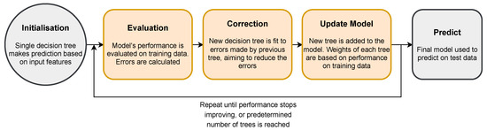
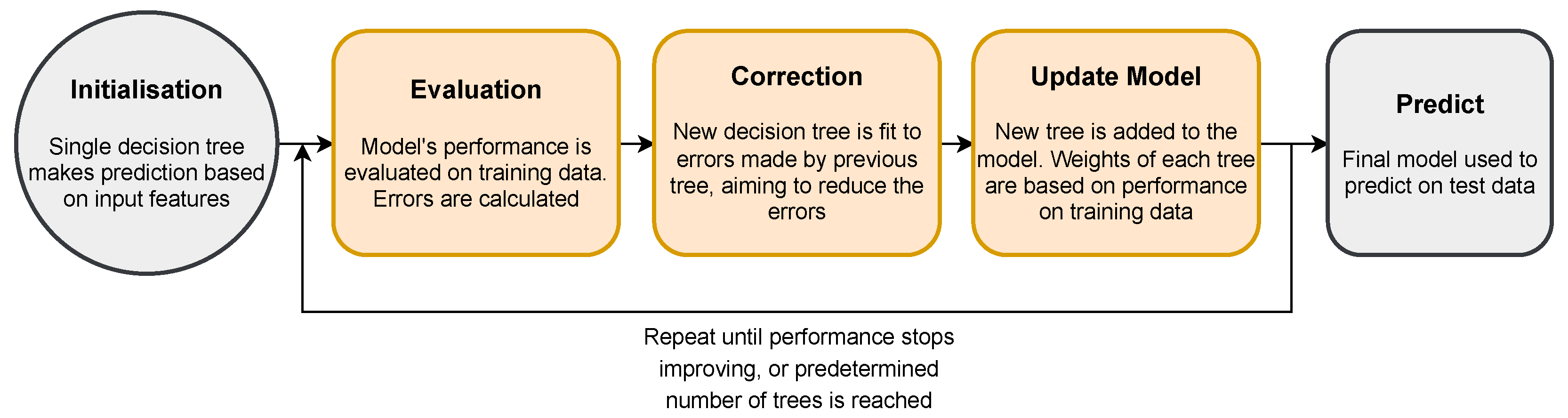
Gradient-boosted decision trees (GBDTs) are popular machine learning algorithms that combine the power of decision trees with the boosting technique, where multiple weak learners are combined in an ensemble to create highly accurate and robust models. Figure 1 depicts the process in which GBDTs build decision trees iteratively, correcting errors of the previous trees in each iteration. Gradient boosting is used to combine the predictions of all the decision trees, with each tree’s contribution weighted according to its accuracy. The final prediction is made by aggregating the predictions of all the decision trees.

Figure 1. XGBoost initialisation, training, and prediction process.

XGBoost, or eXtreme Gradient Boosting [2], is a widely used implementation of GBDTs, used for both classification and regression tasks. XGBoost is designed to be fast, scalable, and highly performant, making it well-suited for large-scale machine learning applications. One of the key features of XGBoost is its use of regularisation functions to prevent overfitting and improve the generalisation of the model. XGBoost also uses a tree pruning algorithm to remove nodes with low feature importance to reduce the complexity of the model and improve accuracy.

XGBoost has been highly successful for tabular data analysis, and deep learning researchers have been striving to surpass its performance.

2.2. Attention and Transformers

Transformers, originating from Vaswani et al. [8], are a type of deep learning architecture originally developed for natural language processing tasks and have been adapted for use in the tabular domain. These models use self-attention to compute the importance of each feature within the context of the entire dataset, enabling them to learn complex, non-linear relationships between features. This is in contrast to GBDTs, where all features are treated equally, and relationships are not considered between them. Attention mechanisms are capable of highlighting relevant features and patterns in the dataset that are the most informative for making accurate predictions.

Multi-head self-attention is a type of attention mechanism used in transformers. A weight is assigned to each input token based on its relevance to the output, allowing selective focus on different parts of the input data.

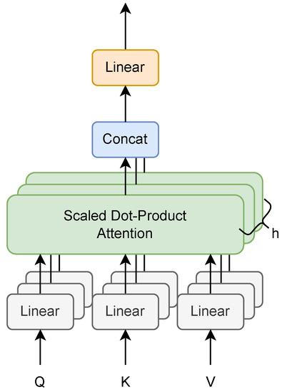
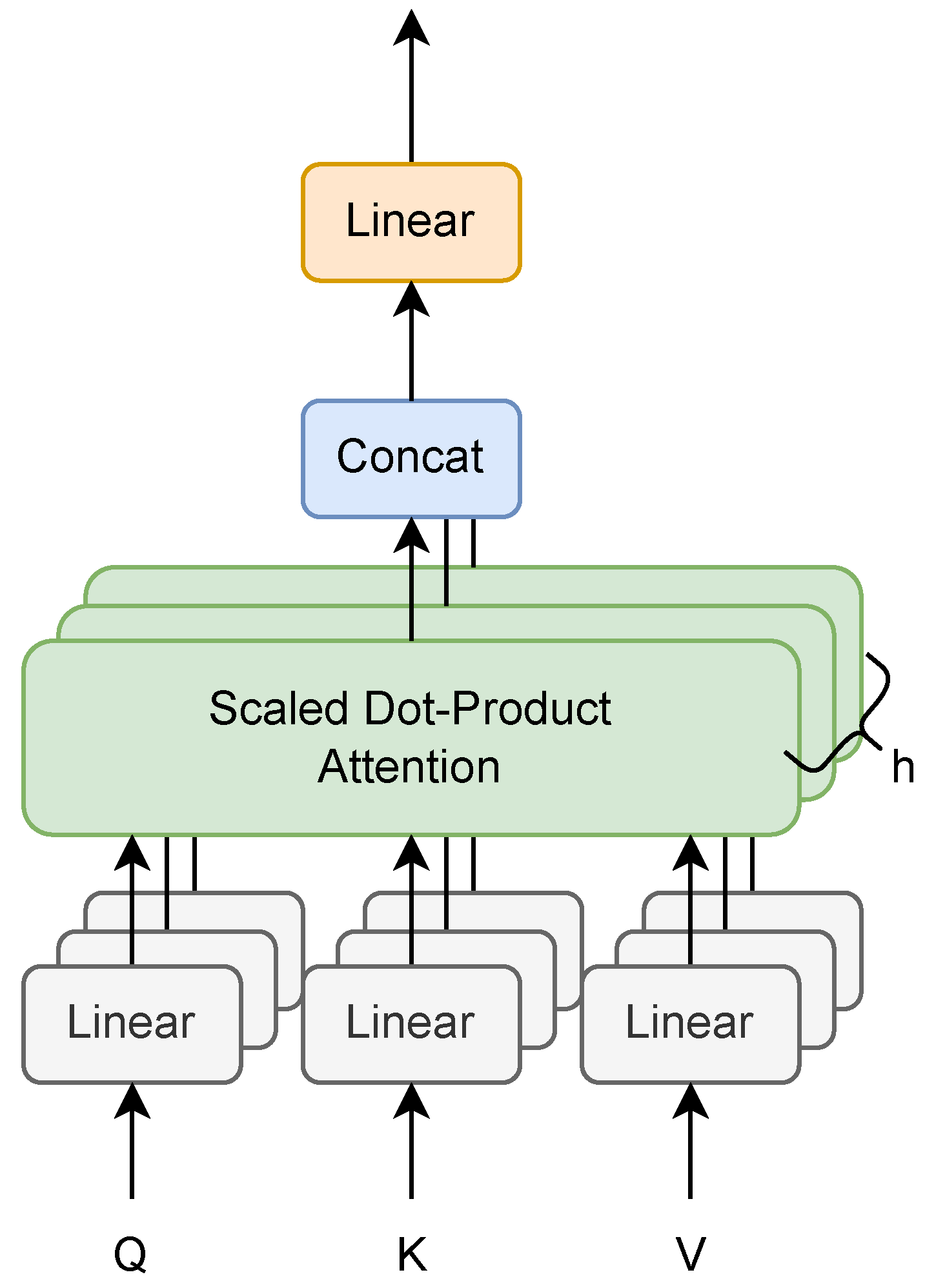
The attention mechanism is applied multiple times in parallel, with each attention head attending to a different subspace of the input representation, allowing the model to capture different aspects of the input data and learn more complex, non-linear relationships between the inputs. The outputs of the multiple attention heads are then concatenated and passed through a linear layer to produce the final output. This is depicted in Figure 2, where the scaled dot-product attention is:

$$Attention(Q,K,V)=softmax(\frac{Q{K}^T}{\sqrt{d_k}})V$$

(1)

Figure 2. Multi-head attention from [8], where h is the number of heads, and Q, K, and V are the query, key, and value vectors.

In Figure 2 and Equation (1), Q, K, and V are the query, key, and value vectors used to compute attention weights between each element of the input sequence. $d_k$ is the dimension of the key vectors.

SAINT [5], the Self-Attention and Intersample Attention Transformer, is a deep learning model designed to make predictions based on tabular data. SAINT utilises attention to highlight specific features or patterns within the dataset that are most relevant for making accurate predictions, helping models better understand complex relationships within the data and make more accurate predictions.

In their experiments, they find that SAINT, on average, outperforms all other methods on supervised and semi-supervised tasks for regression, including GBDT-based methods, on a variety of datasets.

Chemical Kinetics

Siemens Energy developed a Chemical Kinetics PEMS model [7] through mapping emissions via a 1D reactor element code ’GENE-AC’ computational fluid dynamics model of their SGT-400 combustor and converting this to a parametric PEMS model. This is a first-principles-based method that uses factors such as pilot/main fuel split, inlet air temperature, and inlet air pressure to calculate the predicted emissions.

3. Related Works

3.1. Gas Turbine Emissions Prediction

3.1.1. First Principles

Predictive emissions monitoring systems (PEMS) for gas turbines have been developed since 1973 [9], in which an analytical model was developed using thermodynamics to predict NOx emissions. Rudolf et al. [10] developed a mathematical model, which takes into account performance deterioration due to engine ageing. They combined different datasets, such as validation measurements and long-term operational data, to provide more meaningful emission trends. Lipperheide et al. [11] also incorporated ageing of the gas turbines into their analytical model, which is capable of accurately predicting NOx emissions for power in the range of 60–100%. Siemens Energy developed a Chemical Kinetics model [7] to accurately predict CO and NOx emissions for their SGT-400 gas turbine. They used a 1D reactor model to find the sensitivity of the emissions to the different input parameters as a basis for the PEMS algorithm. Bainier et al. [12] monitored their analytical PEMS over two years and found a continuous good level of accuracy, noting that training is required to fully upkeep the system.

3.1.2. Machine Learning

A number of machine learning (ML) methods have been used to predict emissions for gas turbines and have been found to be more flexible for prediction than first-principles methods. Cuccu et al. [13] compared twelve machine learning methods, including linear regression, kernel-based methods, and feed-forward artificial neural networks with different backpropagation methods. They used k-fold cross-validation to select the optimal method-specific parameters, finding that improved resilient backpropagation (iRPROP) achieved the best performance, and note that thorough pre-processing is required to produce such results. Kaya et al. [14] compared three decision fusion schemes on a novel gas turbine dataset, highlighting the importance of certain features within the dataset for prediction. Si et al. [15] also used k-fold validation to determine the optimal hyperparameters for their neural-network-based models. Rezazadeh et al. [16] proposed a k-nearest-neighbour algorithm to predict NOx emissions.

Azzam et al. [17] utilised evolutionary artificial neural networks and support vector machines to model NOx emissions from gas turbines, finding that use of their genetic algorithm results in a high-enough accuracy to offset the computational cost compared to the cheaper support vector machines. Kochueva et al. [18] developed a model based on symbolic regression and a genetic algorithm with a fuzzy classification model to determine “standard” or “extreme” emissions levels to further improve their prediction model. Botros et al. [19,20,21] developed a predictive emissions model based on neural networks with an accuracy of ±10 parts per million.

Guo et al. [22] developed a NOx prediction model based on attention mechanisms, LSTM, and LightGBM. The attention mechanisms were introduced into the LSTM model to deal with the sequence length limitation LSTM faces. They eliminate noise through singular spectrum analysis and then use LightGBM to select the dependent feature. The processed data are then used as input to the LSTM while the attention mechanism enhances the historical learning ability of information. They added feature attention and temporal attention to the LSTM model to improve prediction by allowing different emphases by allocating different weights.

3.1.3. Machine Learning in Industry

Machine learning for other industrial applications has also been found to be useful for prediction. For example, predicting the compressive strength of concrete containing nano silica using support vector machines and Gaussian process regression [23], predicting the mechanical behaviour of 3D-printed components [24], predicting elemental stiffness matrix of functionally graded nanoplates [25], optimising industrial refrigeration systems [26], forecasting strawberry yield [27], and non-intrusive nuclear reactor monitoring [28].

3.2. Tabular Prediction

3.2.1. Tree-Based

Gradient-boosted decision trees (GBDTs) have emerged as the dominant approach for tabular prediction, with deep learning methods only beginning to outperform them in some cases. Notably, XGBoost [2] often achieves state-of-the-art performance in regression problems. Other GBDTs, such as LightGBM [3] and CatBoost [29], have shown success in tabular prediction.

Deep learning faces challenges when dealing with tabular data, such as low-quality training data, the lack of spatial correlation between variables, dependency on preprocessing, and the impact of single features [30]. Shwartz et al. [4] concluded that deep models were weaker than XGBoost, and that deep models only outperformed XGBoost alone when used as an ensemble with XGBoost. They also highlighted the challenges in optimising deep models compared to XGBoost. Grinsztajn et al. [31] found that tree-based models are state of the art on medium-sized data (10,000 samples), especially when taking into account computational cost, due to the specific features of tabular data, such as uninformative features, non-rotationally invariant data, and irregular patterns in the target function. Kadra et al. [32] argued that well-regularised plain MLPs significantly outperform more specialised neural network architectures, even outperforming XGBoost.

3.2.2. Attention and Transformers

Attention- and transformer-based methods have shown promise in recent years for tabular prediction. Ye et al. [33] provided an overview of attention-based approaches for tabular data, highlighting the benefits of attention in tabular models. SAINT [5] introduced intersample attention, which allows rows to attend to each other, as well as using the standard self-attention mechanism, leading to improved performance over GBDTs on a number of benchmark tasks including regression, binary classification and multi-class classification. TabNet [34] is an interpretable model that uses sequential attention to select features to reason from at each step. FT-Transformer [35] is a simple adaption of the Transformer architecture that has outperformed other deep learning solutions on most tasks. However, GBDTs still outperform it on some tasks. TabTransformer [36] transforms categorical features into robust contextual embeddings using transformer layers, but it does not affect continuous variables. Kossen et al. [37] took the entire dataset as input and used self-attention to reason about relationships between data points. ExcelFormer [6] alternated between two attention modules to manipulate feature interactions and feature representation updates and manages to convincingly outperform GBDTs.

Despite the promising results of these attention- and transformer-based methods, deep learning models have generally been weaker than GBDTs on datasets that were not originally used in their respective papers [4]. Proper pre-processing, pre-training [38], and embedding [39] can enable deep learning tabular models to perform significantly better, reducing the gap between deep learning and GBDT models.

4. Materials and Methods

4.1. Data

The data are test bed data from the Siemens SGT400 gas turbines. These are tabular data consisting of a number of different gas turbines tested over a wide range of operating conditions. In total, there are 37,204 rows of data with 183 features, including process parameters such as temperatures and pressures and the target emission variables NOx and CO. All data are numerical values.

4.2. Pre-Processing

From the test bed dataset, two comparison sub-datasets were used: “Full” and “Cropped”. The Cropped dataset consisted of a significant number of filters pre-applied to the data by Siemens Energy for the Chemical Kinetics model, while the Full dataset had no filters applied. Standard pre-processing was applied to both sets of data including removing rows with missing data, removing negatives from emissions data, and removing liquid fuel data. Features with a significant number of missing rows were also removed. For the Full dataset, any features with more than 18,100 missing values were removed. Similarly, for the Cropped dataset, features with more than 3000 missing values were removed. These threshold values were chosen to be greater than the number of missing values than the maximum number of missing values found in the emission columns.

Table 1 provides an overview of both sub-datasets and the number of rows and features in each. Due to the prior pre-processing removing proportionally more missing values through the original filters, the Cropped dataset ends with more rows of data compared to the Full dataset, at the cost of reducing the number of features. When removing the same features from the Cropped dataset as the Full dataset, only 2044 rows remain, so this was not chosen to be used for modelling.

Table 1. Pre-processing process for the Full and Cropped datasets showing number of rows in each dataset.

Action	Full	Cropped
Start	37,204 rows, 183 features	9873 rows, 183 features
Remove low data features	Removes 9 features	Removes 95 features
Remove liquid fuel data	Removes 5752 rows	No change
Remove negative emissions	Removes 16,977 rows	Removes 744 rows
Remove all missing values	Removes 8615 rows	Removes 2700 rows
End	5860 rows, 174 features	6429 rows, 88 features

We used XGBoost’s feature importance to order each feature from most to least important to create sub-datasets for both the Full and Cropped datasets. The most important features for the Full dataset were Compressor exit pressure and turbine interduct temperature. The most important features of the Cropped dataset were the main/pilot burner split and a pilot-tip temperature. Further feature details including each feature’s importance can be found in Table A1.

The dataset is collected from 0% to 126% load, and pre-processing reduces this to 24% to 126%. We utilise this full range for our comparisons.

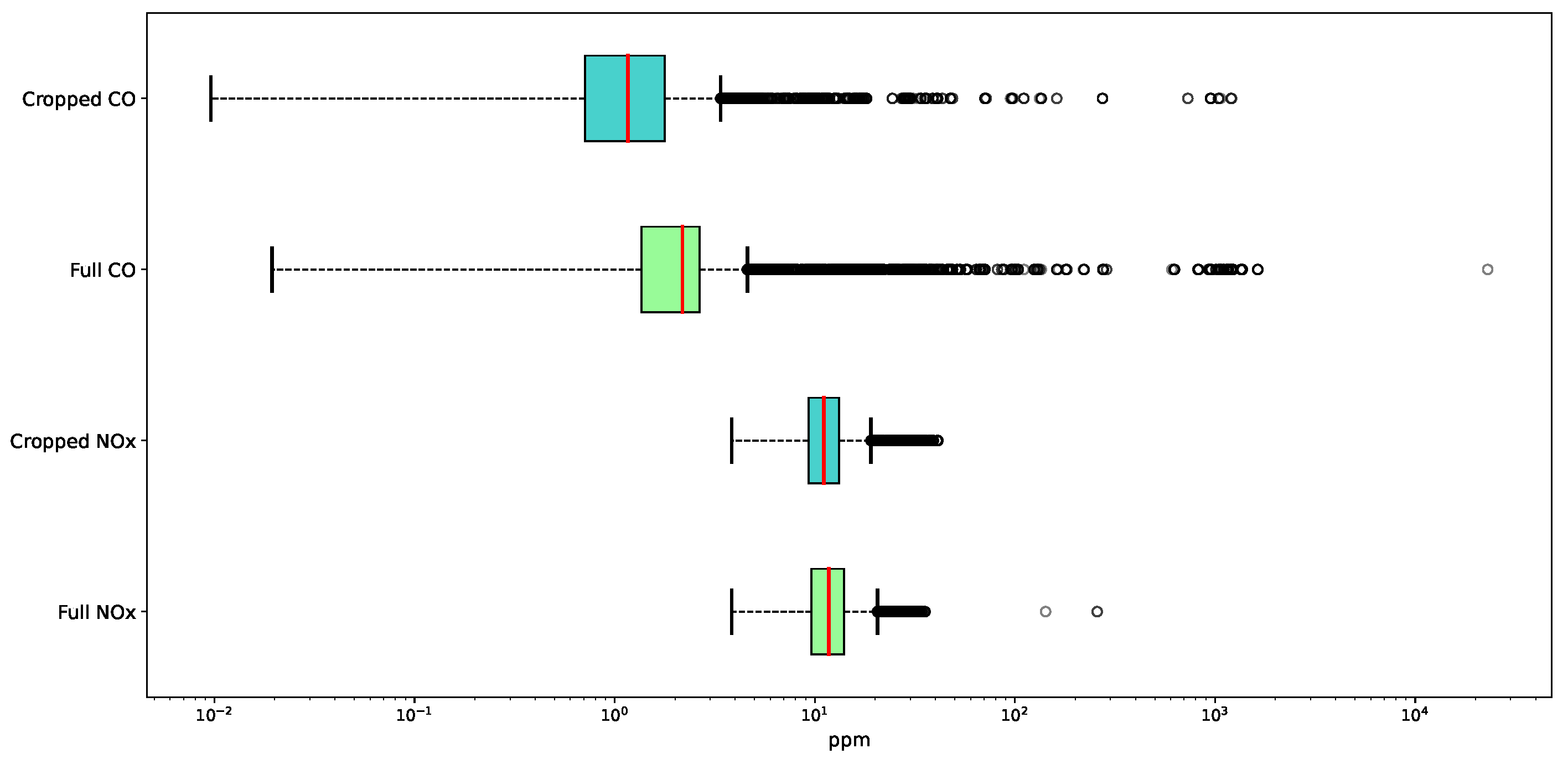
Figure 3 depicts the spread of the data for the target emissions, NOx and CO, for both sub-datasets. CO has many more outliers compared to NOx, with some particularly far from the median.

Figure 3. NOx and CO data spread for Full and Cropped datasets on a logarithmic scale.

4.3. Models

We compared a transformer-based model, SAINT [5], and GBDT XGBoost [2], against the existing PEMS model used by Siemens Energy, a first-principles-based Chemical Kinetics model [7]. These models were both chosen due to their excellent prior performance on tabular prediction on baseline models and on our preliminary study into gas turbine emissions prediction [1].

4.3.1. SAINT

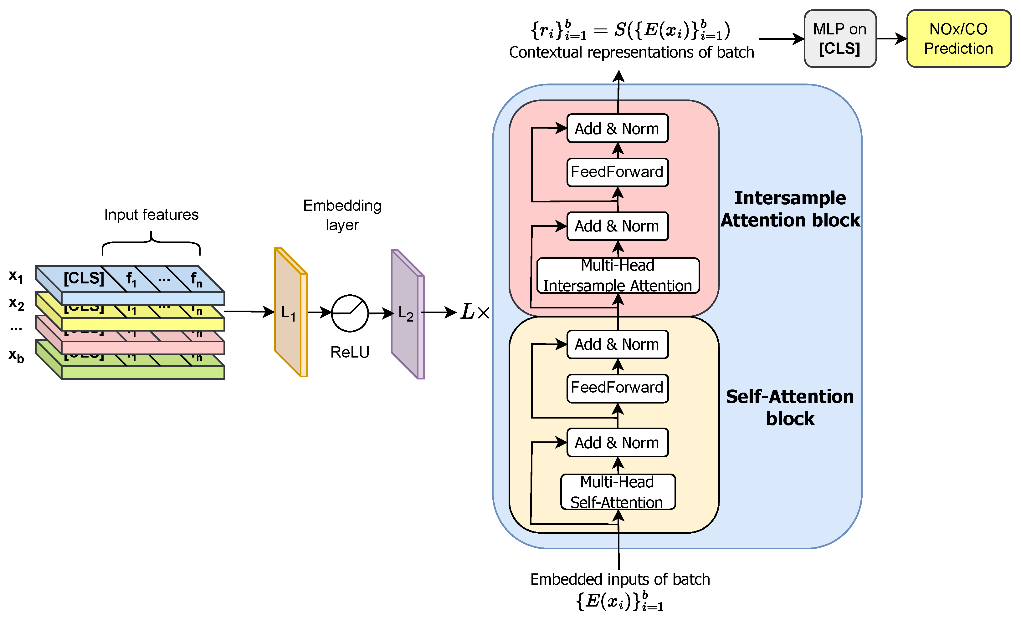
Figure 4 depicts the SAINT method. The features, [$f_1,\dots ,f_n$], are the process parameters from sensors within the gas turbine tests, where n is the number of features. Each $x_i$ is one row of data, including one of each feature, where b is the batch size, 32. A [CLS] token with a learned embedding is appended to each data sample. This batch of inputs is passed through an embedding layer, consisting of a linear layer, a ReLU non-linearity, followed by a linear layer, prior to being processed by the SAINT model L times, where L is 3. Only representations corresponding to the [CLS] token are selected for an MLP to be applied to. MSE loss is achieved on predictions during training. For our experiment, n is the number of features for each experiment. $L_1$ is the first linear layer, with 1 input feature and 100 output features, and $L_2$ is the second linear layer, with 100 input features and 1 output feature. The embedding layer is performed for each feature.

Figure 4. Proposed method based on SAINT [5].

SAINT accepts a sequence of feature embeddings as input and produces contextual representations with the same dimensionality.

Features are projected into a combined dense vector space and passed as tokens into a transformer encoder. A single fully connected layer with a ReLU activation is used for each continuous feature’s embedding.

SAINT alternates self-attention and intersample attention mechanisms to enable the model to attend to information over both rows and columns. The self-attention attends to individual features within each data sample, and intersample attention relates each row to other rows in the input, allowing all features from different samples to communicate with each other.

Similar to the original transformer [8], there are L identical layers, each containing one self-attention and one intersample attention transformer block. The self-attention block is identical to the encoder from [8], consisting of a multi-head self-attention layer with 8 heads, and two fully connected feed-forward layers with a GELU non-linearity. A skip connection and layer normalisation are applied to each layer. The self-attention layer is replaced by an intersample attention layer for the intersample attention block. For the intersample attention layer, the embeddings of each feature are concatenated for each row, and attention is computed over samples rather than features, allowing communication between samples.

As described in the original work [5], $\mathcal{D}={\{x_i,y_i\}}_{i=1}^m$ is a tabular dataset with m points, $x_i$ is an n-dimensional feature vector of process parameters, and $y_i$ is a target emission value. A $\left[CLS\right]$ token is appended with a learned embedding to each sample, such that $x_i=[\left[CLS\right], f_i^1, f_i^2, \dots , f_i^n]$ is a single data point with continuous features $f_i^{\left\{j\right\}}$, and E is the embedding layer which embeds each feature into ${\mathbb{R}}^d$.

The SAINT pipeline is described as follows for a batch of b inputs, where MSA is multi-head self-attention, MISA is multi-head intersample attention, LN is layer norm, and FF is feed-forward layer:

$$z_i^{(1)}=LN(MSA(\mathbf{E}(x_i)))+\mathbf{E}(x_i)$$

(2)

$$z_i^{(2)}=LN(F{F}_1(z_i^{(1)}))+z_i^{(1)}$$

(3)

$$z_i^{(3)}=LN(MISA({\left\{z_i^{(2)}\right\}}_{i=1}^b))+z_i^{(2)}$$

(4)

$$r_i=LN(F{F}_2(z_i^{(3)}))+z_i^{(3)}$$

(5)

where $r_i$ is SAINT’s contextual representation output corresponding to data point $x_i$, which can be used in downstream tasks.

We use SAINT, as seen in Figure 4, in a fully supervised multivariate regression setting. The code we based our experiments on can be found at (https://github.com/somepago/saint, accessed on 14 February 2023). We used the AdamW optimiser with a learning rate of 0.0001.

4.3.2. XGBoost

XGBoost reduces overfitting through regularisation and pruning, using a distributed gradient boosting algorithm to optimise the model’s objective function to make it more scalable and efficient, and automatically handles missing values.

Decision trees are constructed in a greedy manner as a weak learner. At each iteration, XGBoost evaluates the performance of the current ensemble and adds a new tree to the ensemble that minimises the loss function through gradient descent. Each successive tree implemented compensates for residual errors in the previous tree.

4.3.3. Chemical Kinetics

We compared our work to an updated Chemical Kinetics model, based on [7], using the same sets of test data for comparisons. The predictions for the Chemical Kinetics model are essentially part of the original dataset, with the number of features and rows of each sub-dataset, described in Section 4.2, not affecting the raw predictions but eliminating the varying rows depending on missing values due to features in the dataset.

4.4. Metrics and Evaluation

The metrics used to evaluate the models in this work are the mean absolute error (MAE) and root mean squared error (RMSE).

MAE is expressed as follows:

$$MAE=\frac{1}{n}\sum _{i=1}^n|y_i-\widehat{y_i}|$$

(6)

RMSE is expressed as follows:

$$RMSE=\sqrt{\frac{1}{n}\sum _{i=1}^n{(y_i-\widehat{y_i})}^2}$$

(7)

We used randomised cross-validation to evaluate the performance of the machine learning models, SAINT and XGBoost, whereby the data were randomly sub-sampled 10 times to obtain unbiased estimates of the models’ performance on new, unseen data on which they were re-trained and tested. We report the average and standard deviation of the MAE and RMSE for each sub-dataset, providing insight into the models’ consistency and variation in performance. The Chemical Kinetics model is also compared on these test sets to provide a relative benchmark for the performance of the models. The CO and NOx emissions targets are individually trained to achieve specialised models for each target.

4.5. Impact of Number of Features

To assess the influence of the number of features compared to the number of rows of data on prediction performance, we further split each dataset where each subset contained a decreasing number of features, leading to fewer rows of missing data, allowing an examination into the effect of removing less important features on the availability of data points for training. Feature removal followed the order of decreasing feature importance according to XGBoost, where the importance is calculated by XGBoost based on how often each feature is used to make key decisions across all trees in the ensemble. The order of importance for each feature can be found in Table A1.

5. Results and Discussion

Table 2 describes the average MAE and RMSE obtained from the 10 sub-samples of the dataset with a varying number of features. XGBoost has on average the lowest MAE for each emission and number of features, while SAINT has a lower RMSE on average. SAINT and XGBoost have MAE results close to each other compared to the Chemical Kinetics model for NOx. For example, with 174 features, SAINT has an MAE of 0.91, XGBoost has 0.62, and Chemical Kinetics has 4.46, and this trend continues for all numbers of features. For CO, XGBoost significantly outperforms both SAINT and the Chemical Kinetics model for MAE, with an MAE of 5.05 for 174 features compared to 11.37 for SAINT, and the Chemical Kinetics model is several orders of magnitude higher. However, the standard deviation for all models is much higher for CO too. The lower RMSE from SAINT in most situations suggests it is better at handling outliers compared to XGBoost.

Table 2. Tabular prediction results for each model on the two sets of data and four sets of number of features used. Mean value for 10 dataset subsamples provided with standard deviation.

Methods		SAINT		XGBoost		Chemical Kinetic
Metric		MAE	RMSE	MAE	RMSE	MAE	RMSE
NOx Full	174	0.91 ± 0.11	2.82 ± 2.45	0.62 ± 0.14	4.08 ± 3.09	4.46 ± 0.15	6.59 ± 1.43
	130	0.89 ± 0.21	2.92 ± 2.02	0.74 ± 0.18	4.48 ± 3.65	4.09 ± 0.10	6.14 ± 1.14
	87	1.72 ± 0.70	3.83 ± 1.62	0.76 ± 0.12	4.04 ± 2.62	4.09 ± 0.10	6.14 ± 1.14
	45	1.14 ± 0.38	2.96 ± 1.64	0.74 ± 0.08	3.00 ± 1.99	3.68 ± 0.12	5.55 ± 0.94
NOx Cropped	88	0.54 ± 0.08	0.92 ± 0.1	0.47 ± 0.02	0.95 ± 0.17	2.67 ± 0.06	3.84 ± 0.33
	45	0.56 ± 0.07	0.94 ± 0.07	0.44 ± 0.02	0.92 ± 0.16	2.67 ± 0.06	3.84 ± 0.33
CO Full	174	11.37 ± 6.61	117.61 ± 191.07	5.05 ± 6.45	117.83 ± 197.50	2.49 × 10${}^6$ ± 7.54 × 10${}^5$	3.79 × 10${}^7$ ± 7.35 × 10${}^6$
	130	10.58 ± 5.84	164.20 ± 225.07	7.41 ± 8.09	220.53 ± 260.67	1.47 × 10${}^6$ ± 5.98 × 10${}^5$	2.85 × 10${}^7$ ± 7.37 × 10${}^6$
	87	14.31 ± 6.33	152.70 ± 225.24	7.68 ± 10.80	214.44 ± 317.08	1.50 × 10${}^6$ ± 5.98 × 10${}^5$	2.85 × 10${}^7$ ± 7.37 × 10${}^6$
	45	24.97 ± 30.58	292.55 ± 236.71	6.04 ± 6.30	219.92 ± 262.52	1.38 × 10${}^6$ ± 8.93 × 10${}^5$	2.64 × 10${}^7$ ± 1.28 × 10${}^7$
CO Cropped	88	2.46 ± 0.72	20.02 ± 10.14	0.59 ± 0.31	9.13 ± 8.15	5.97 × 10${}^5$ ± 3.32 × 10${}^5$	1.80 × 10${}^7$ ± 9.34 × 10${}^6$
	45	2.73 ± 2.30	20.01 ± 10.15	0.63 ± 0.37	10.50 ± 9.31	5.96 × 10${}^5$ ± 3.32 × 10${}^5$	1.80 × 10${}^7$ ± 9.34 × 10${}^6$

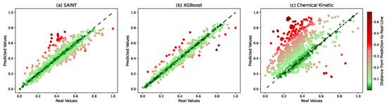
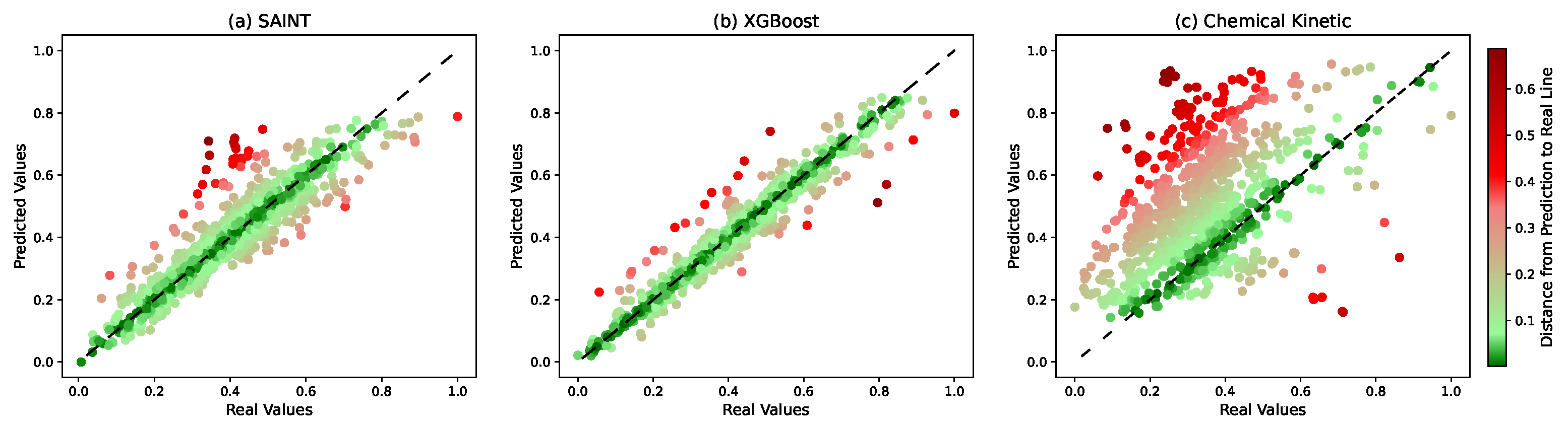
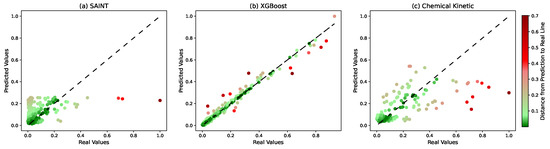
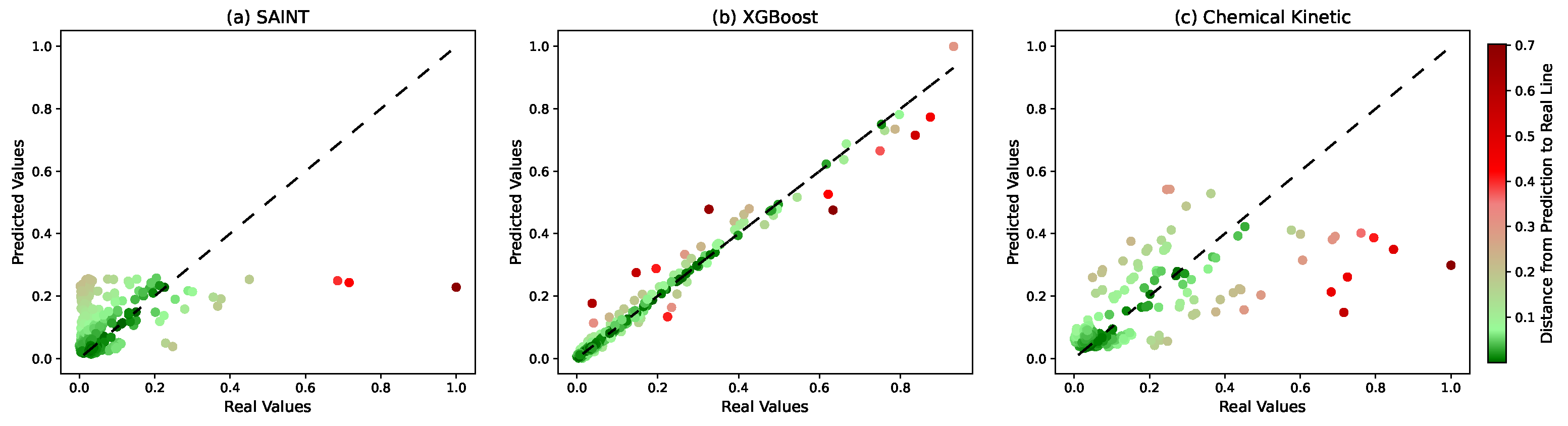
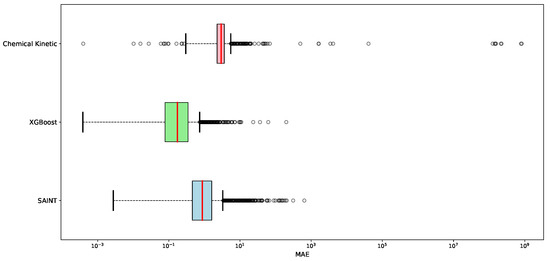
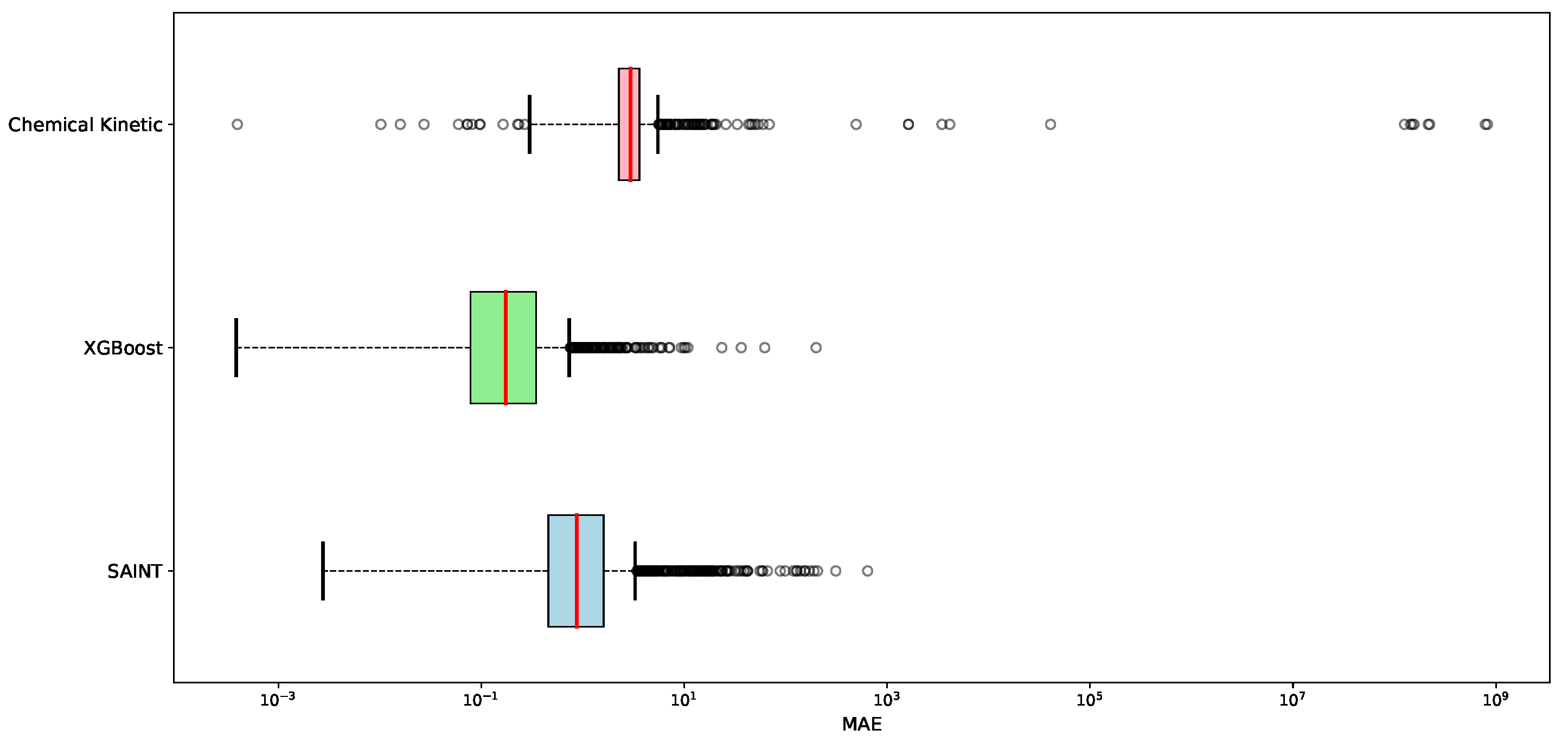
Figure 5 and Figure 6 show the normalised predictions compared to the real values for NOx and CO. For Figure 6, the predictions above 1000 ppm were removed from view as these were extremely anomalous and prevented the main results from being seen clearly. For both emissions, the Chemical Kinetics model has significantly more spread compared to SAINT and XGBoost. SAINT and XGBoost both follow the identity line closely for NOx, showing that most predictions are within an accurate range for both low and high emissions. For CO especially, XGBoost predictions are closer to the identity line compared to SAINT. SAINT does not predict the higher emissions values for CO as well as XGBoost does, with the largest real CO values not being predicted well at all, but it does manage to closely predict the majority of the emissions. This is highlighted in Figure 7 where SAINT has a low median MAE with more and larger outlier errors compared to XGBoost.

Figure 5. Normalised real vs. predicted values for NOx for each model within one standard deviation.

Figure 6. Normalised real vs. predicted values for CO for each model within one standard deviation for the Full dataset with all features. Extreme anomalous real and predicted values above 1000 were also removed, removing 14 data points.

Figure 7. Box plots for MAE results for CO for each model on a logarithmic scale.

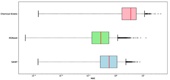
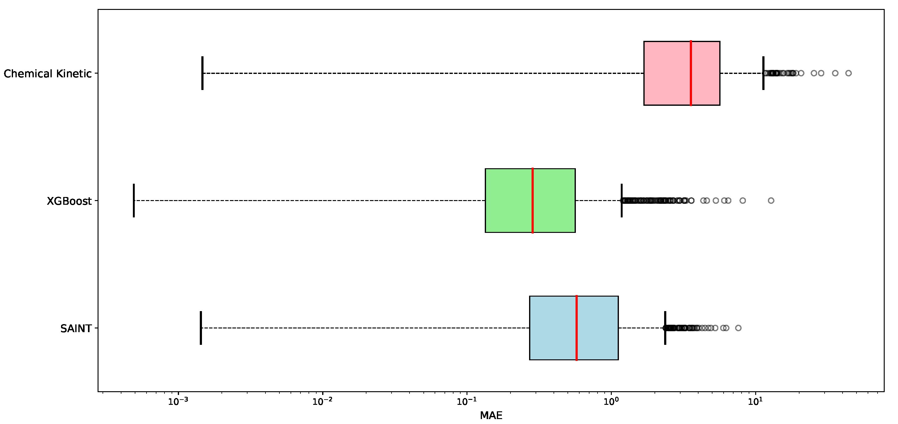
All models, especially the Chemical Kinetics model, have significant errors when predicting CO. Further analysis of these results indicated that these large errors were primarily driven by a small number of data points with extremely anomalous MAE values. Figure 7 and Figure 8 illustrate these outliers, with the logarithmic scale emphasising the limited number of data points responsible for the higher mean MAE. Despite the presence of outliers, the median MAE values for each model were not excessively high, with the majority of data points exhibiting more accurate predictions for CO.

Figure 8. Box plots for MAE results for NOx for each model on a logarithmic scale.

Figure 6 demonstrates that the majority of predictions generated by all models fall within a reasonable range for accurate CO emission prediction for gas turbines. While overall performance may be affected by the presence of outliers, the models do exhibit good predictive capabilities for CO and NOx emissions.

In our evaluation, XGBoost provided the best prediction accuracy for both NOx and CO, with both machine learning methods outperforming the original Chemical Kinetics model. Prediction for NOx is significantly more accurate than CO prediction for all models. This can be attributed to the wider spread of data points and greater presence of influential outliers in the CO real values, as evident in Figure 3. The abundance of outliers in the CO dataset made it inherently more challenging to predict accurately. The filters used for the Cropped dataset particularly improved the RMSE of the machine learning models as it removed some outlier inputs in the dataset such that outliers would have a smaller impact.

5.1. Impact of Pre-Processing

The Cropped dataset consistently outperformed the Full dataset, suggesting that careful and specific pre-processing is important for good prediction for gas turbine emissions. As seen in Table 2, the standard deviation is significantly reduced when using the Cropped dataset compared to Full, likely due to the extreme emissions values being removed such that there is a smaller possibility for prediction. However, this may not be useful in the long run for emissions prediction as real-life operational data will have anomalous and varied data as in the test bed dataset, so using the Full dataset may provide a more generalisable model.

5.2. Number of Features: Impact and Importance

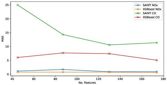
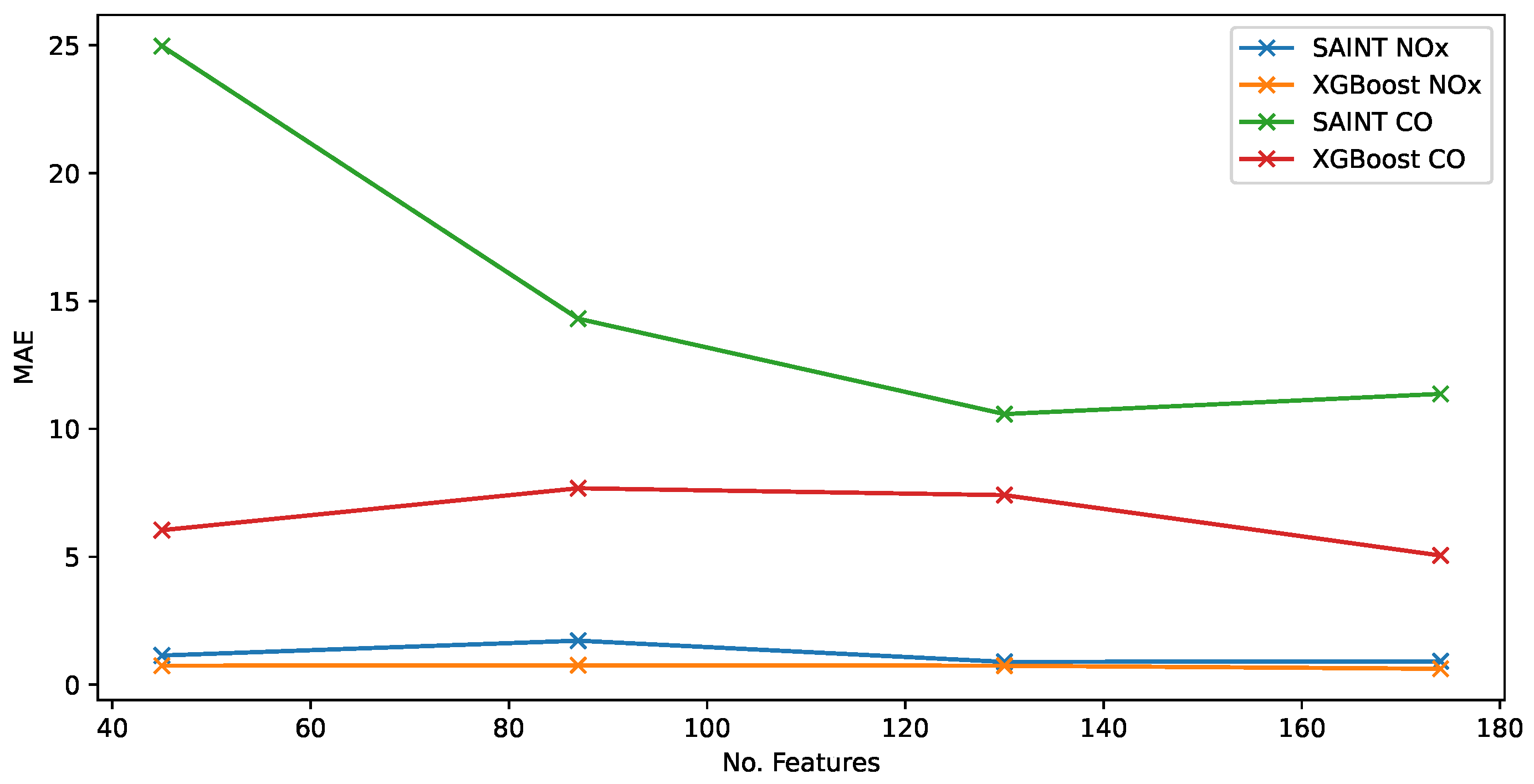
Figure 9 displays the relationship between the MAE values and the number of features in the analysis for the Full dataset, highlighting the potential impact of feature removal and its effect on prediction performance. This provides further insights as to the feature importance that can be seen in Table A1. For training, on average, between the 10 sub-datasets, there were 3808 rows with 174 features, 5084 rows for 130 and 87 features, and 6223 rows for 45 features.

Figure 9. MAE compared to number of features for the Full dataset.

From this figure, it appears that the number of features and number of rows does not significantly affect the MAE. Given that the sub-datasets with 130 and 87 features had the same rows of data and that these extra features did not impact the prediction results significantly, this may suggest that the models largely rely on the most important features in the datasets, and the extra ones are less relevant for prediction. Therefore, from a practical standpoint, the sweet spot in terms of performance is achieved with 45 features. Further restricting the dataset to fewer high-importance features may provide further insight into this finding.

6. Conclusions and Future Work

We have compared two machine learning models, SAINT and XGBoost, against an industry-used Chemical Kinetics model for gas turbine emissions prediction to demonstrate improved predictive performance for both NOx and CO and to determine whether a deep learning-based model or gradient-boosted decision tree model performed the best for this task. XGBoost remained the best model for tabular prediction for this gas turbine dataset for both NOx and CO, but the deep-learning-based model, SAINT, is catching up in terms of performance, with lower RMSE scores indicating better outlier handling. Both machine learning models outperformed the first-principles-based Chemical Kinetics model, indicating that machine learning continues to show a promising future for gas turbine emissions prediction. We also considered the impact of the number of features used in the dataset leading to fewer rows of data available due to increasing missing values in each column and found that increasing features available did not significantly impact the predictive capability of SAINT or XGBoost, potentially indicating that the high-importance features are the most relevant for prediction.

Furthermore, to fully utilise the years of operational gas turbine data that is available but unlabelled, a future step to improve gas turbine emissions prediction will be to include self-supervised learning into the training process. Despite XGBoost displaying the best performance here, attention-based deep learning methods such as SAINT will be easier to combine with self-supervised learning by performing a pretext task such as masking to predict masked sections of the operational data to learn representations of the data, which can then be used in a downstream task using SAINT to create predictions.

References

- Potts, R.L.; Leontidis, G. Attention-Based Deep Learning Methods for Predicting Gas Turbine Emissions. In Proceedings of the Northern Lights Deep Learning Conference 2023 (Extended Abstracts), Tromso, Norway, 9–13 January 2023. [Google Scholar]
- Chen, T.; Guestrin, C. Xgboost: A scalable tree boosting system. In Proceedings of the 22nd ACM Sigkdd International Conference on Knowledge Discovery and Data Mining, New York, NY, USA, 13–17 August 2016; pp. 785–794. [Google Scholar]
- Ke, G.; Meng, Q.; Finley, T.; Wang, T.; Chen, W.; Ma, W.; Ye, Q.; Liu, T.-Y. Lightgbm: A highly efficient gradient boosting decision tree. Adv. Neural Inf. Process. Syst. 2017, 30. [Google Scholar]
- Shwartz-Ziv, R.; Armon, A. Tabular data: Deep learning is not all you need. Inf. Fusion 2022, 81, 84–90. [Google Scholar]
- Somepalli, G.; Schwarzschild, A.; Goldblum, M.; Bruss, C.B.; Goldstein, T. SAINT: Improved neural networks for tabular data via row attention and contrastive pre-training. In NeurIPS 2022 First Table Representation Workshop; NeurIPS: London, UK, 2022. [Google Scholar]
- Chen, J.; Yan, J.; Chen, D.Z.; Wu, J. Excelformer: A neural network surpassing gbdts on tabular data. arXiv 2023, arXiv:2301.02819. [Google Scholar]
- Hackney, R.; Sadasivuni, S.; Rogerson, J.; Bulat, G. Predictive emissions monitoring system for small siemens dry low emissions combustors: Validation and application. In Turbo Expo: Power for Land, Sea, and Air; American Society of Mechanical Engineers: New York, NY, USA, 2016; Volume 49767, p. V04BT04A032. [Google Scholar]
- Vaswani, A.; Shazeer, N.; Parmar, N.; Uszkoreit, J.; Jones, L.; Gomez, A.N.; Kaiser, Ł.; Polosukhin, I. Attention is all you need. In Proceedings of the Advances in Neural Information Processing Systems 30 (NIPS 2017), Long Beach, CA, USA, 4–9 December 2017. [Google Scholar]
- Hung, W. An experimentally verified nox emission model for gas turbine combustors. In Turbo Expo: Power for Land, Sea, and Air; American Society of Mechanical Engineers: New York, NY, USA, 1975; Volume 79771, p. V01BT02A009. [Google Scholar]
- Rudolf, C.; Wirsum, M.; Gassner, M.; Zoller, B.T.; Bernero, S. Modelling of gas turbine nox emissions based on long-term operation data. In Turbo Expo: Power for Land, Sea, and Air; American Society of Mechanical Engineers: New York, NY, USA, 2016; Volume 49767, p. V04BT04A006. [Google Scholar]
- Lipperheide, M.; Weidner, F.; Wirsum, M.; Gassner, M.; Bernero, S. Long-term nox emission behavior of heavy duty gas turbines: An approach for model-based monitoring and diagnostics. J. Eng. Gas Turbines Power 2018, 140, 101601. [Google Scholar]
- Bainier, F.; Alas, P.; Morin, F.; Pillay, T. Two years of improvement and experience in pems for gas turbines. In Turbo Expo: Power for Land, Sea, and Air; American Society of Mechanical Engineers: New York, NY, USA, 2016; Volume 49873, p. V009T24A005. [Google Scholar]
- Cuccu, G.; Danafar, S.; Cudré-Mauroux, P.; Gassner, M.; Bernero, S.; Kryszczuk, K. A data-driven approach to predict nox-emissions of gas turbines. In Proceedings of the 2017 IEEE International Conference on Big Data (Big Data), Boston, MA, USA, 11–14 December 2017; pp. 1283–1288. [Google Scholar]
- Kaya, H.; Tüfekci, P.; Uzun, E. Predicting co and nox emissions from gas turbines: Novel data and a benchmark pems. Turk. J. Electr. Eng. Comput. Sci. 2019, 27, 4783–4796. [Google Scholar] [CrossRef] [Scilit]
- Si, M.; Tarnoczi, T.J.; Wiens, B.M.; Du, K. Development of predictive emissions monitoring system using open source machine learning library–keras: A case study on a cogeneration unit. IEEE Access 2019, 7, 113463–113475. [Google Scholar]
- Rezazadeh, A. Environmental pollution prediction of nox by process analysis and predictive modelling in natural gas turbine power plants. arXiv 2020, arXiv:2011.08978. [Google Scholar]
- Azzam, M.; Awad, M.; Zeaiter, J. Application of evolutionary neural networks and support vector machines to model nox emissions from gas turbines. J. Environ. Chem. Eng. 2018, 6, 1044–1052. [Google Scholar] [CrossRef] [Scilit]
- Kochueva, O.; Nikolskii, K. Data analysis and symbolic regression models for predicting co and nox emissions from gas turbines. Computation 2021, 9, 139. [Google Scholar] [CrossRef] [Scilit]
- Botros, K.; Selinger, C.; Siarkowski, L. Verification of a neural network based predictive emission monitoring module for an rb211-24c gas turbine. In Turbo Expo: Power for Land, Sea, and Air; American Society of Mechanical Engineers: New York, NY, USA, 2009; Volume 48869, pp. 431–441. [Google Scholar]
- Botros, K.; Cheung, M. Neural network based predictive emission monitoring module for a ge lm2500 gas turbine. In Proceedings of the International Pipeline Conference, Calgary, AB, Canada, 27 September–1 October 2010; Volume 44229, pp. 77–87. [Google Scholar]
- Botros, K.; Williams-Gossen, C.; Makwana, S.; Siarkowski, L. Predictive emission monitoring (pem) systems development and implementation. In Proceedings of the 19th Symposium on Industrial Applications of Gas Turbines Committee, Banff, AB, Canada, 17–19 October 2011. [Google Scholar]
- Guo, L.; Zhang, S.; Huang, Q. Nox prediction of gas turbine based on dual attention and lstm. In Proceedings of the 2022 34th Chinese Control and Decision Conference (CCDC), Hefei, China, 15–17 August 2022; pp. 4036–4041. [Google Scholar]
- Garg, A.; Aggarwal, P.; Aggarwal, Y.; Belarbi, M.; Chalak, H.; Tounsi, A.; Gulia, R. Machine learning models for predicting the compressive strength of concrete ontaining nano silica. Comput. Concr. 2022, 30, 33. [Google Scholar]
- Nasiri, S.; Khosravani, M. Machine learning in predicting mechanical behavior of additively manufactured parts. J. Mater. Res. Technol. 2021, 14, 1137–1153. [Google Scholar] [CrossRef] [Scilit]
- Garg, A.; Belarbi, M.; Tounsi, A.; Li, L.; Singh, A.; Mukhopadhyay, T. Predicting elemental stiffness matrix of FG nanoplates using Gaussian Process Regression based surrogate model in framework of layerwise model. Eng. Anal. Bound. Elem. 2022, 143, 779–795. [Google Scholar] [CrossRef] [Scilit]
- Onoufriou, G.; Bickerton, R.; Pearson, S.; Leontidis, G. Nemesyst: A hybrid parallelism deep learning-based framework applied for internet of things enabled food retailing refrigeration systems. Comput. Ind. 2019, 113, 103133. [Google Scholar] [CrossRef] [Scilit]
- Onoufriou, G.; Hanheide, M.; Leontidis, G. Premonition Net, a multi-timeline transformer network architecture towards strawberry tabletop yield forecasting. Comput. Electron. Agric. 2023, 208, 107784. [Google Scholar] [CrossRef] [Scilit]
- Durrant, A.; Leontidis, G.; Kollias, S.; Torres, A.; Montalvo, C.; Mylonakis, A.; Demaziere, C.; Vinai, P. Detection and localisation of multiple in-core perturbations with neutron noise-based self-supervised domain adaptation. In Proceedings of the International Conference on Mathematics and Computational Methods Applied to Nuclear Science and Engineering (M&C2021), Online, 3–7 October 2021. [Google Scholar]
- Prokhorenkova, L.; Gusev, G.; Vorobev, A.; Dorogush, A.V.; Gulin, A. Catboost: Unbiased boosting with categorical features. Adv. Neural Inf. Process. Syst. 2018, 31. [Google Scholar]
- Borisov, V.; Leemann, T.; Seßler, K.; Haug, J.; Pawelczyk, M.; Kasneci, G. Deep neural networks and tabular data: A survey. IEEE Trans. Neural Netw. Learn. Syst. 2022, 1–21. [Google Scholar] [CrossRef] [Scilit]
- Grinsztajn, L.; Oyallon, E.; Varoquaux, G. Why do tree-based models still outperform deep learning on tabular data? arXiv 2022, arXiv:2207.08815. [Google Scholar]
- Kadra, A.; Lindauer, M.; Hutter, F.; Grabocka, J. Well-tuned simple nets excel on tabular datasets. Adv. Neural Inf. Process. Syst. 2021, 34, 23928–23941. [Google Scholar]
- Ye, A.; Wang, A. Applying attention to tabular data. In Modern Deep Learning for Tabular Data: Novel Approaches to Common Modeling Problems; Springer: Berlin/Heidelberg, Germany, 2022; pp. 452–548. [Google Scholar]
- Arik, S.Ö.; Pfister, T. Tabnet: Attentive interpretable tabular learning. Proc. AAAI Conf. Artif. Intell. 2021, 35, 6679–6687. [Google Scholar] [CrossRef] [Scilit]
- Gorishniy, Y.; Rubachev, I.; Khrulkov, V.; Babenko, A. Revisiting deep learning models for tabular data. Adv. Neural Inf. Process. Syst. 2021, 34, 18932–18943. [Google Scholar]
- Huang, X.; Khetan, A.; Cvitkovic, M.; Karnin, Z. Tabtransformer: Tabular data modeling using contextual embeddings. arXiv 2020, arXiv:2012.06678. [Google Scholar]
- Kossen, J.; Band, N.; Lyle, C.; Gomez, A.N.; Rainforth, T.; Gal, Y. Self-attention between datapoints: Going beyond individual input-output pairs in deep learning. Adv. Neural Inf. Process. Syst. 2021, 34, 28742–28756. [Google Scholar]
- Rubachev, I.; Alekberov, A.; Gorishniy, Y.; Babenko, A. Revisiting pretraining objectives for tabular deep learning. arXiv 2022, arXiv:2207.03208. [Google Scholar]
- Gorishniy, Y.; Rubachev, I.; Babenko, A. On embeddings for numerical features in tabular deep learning. Adv. Neural Inf. Process. Syst. 2022, 35, 24991–25004. [Google Scholar]
Disclaimer/Publisher’s Note: The statements, opinions and data contained in all publications are solely those of the individual author(s) and contributor(s) and not of MDPI and/or the editor(s). MDPI and/or the editor(s) disclaim responsibility for any injury to people or property resulting from any ideas, methods, instructions or products referred to in the content. |
© 2023 by the authors. Licensee MDPI, Basel, Switzerland. This article is an open access article distributed under the terms and conditions of the Creative Commons Attribution (CC BY) license (https://creativecommons.org/licenses/by/4.0/).