


Abstract
Metal-coated polymer electrodes fabricated by additive manufacturing are promising tools for electrical discharge machining (EDM) of complex shapes; however, coating non-uniformity and thermomechanical degradation limit their performance. This study presents experimental and theoretical results for a hybrid tool electrode fabricated by stereolithography (SLA), followed by electroless and electrochemical copper plating, and used to machine St3 structural steel. Optical and scanning electron microscopy, energy-dispersive spectroscopy (EDS), atomic force microscopy, X-ray microtomography, Raman spectroscopy, simultaneous thermal analysis and nanoindentation were used to characterize the coating before and after EDM. The electroplated copper layer exhibited pronounced thickness non-uniformity (264–1225 µm), an edge effect and dendritic morphology associated with the primary current distribution and the absence of leveling additives. Surface modification during EDM was accompanied by changes in the elemental composition measured by EDS. After EDM, the Fe and C signals reached 23.32 wt.% and 35.56 wt.%, respectively, under the acquisition and quantification conditions used. These values characterize local surface composition and do not establish bulk incorporation of iron or carbon into the copper layer. No pronounced bulk thermal degradation was detected in the examined photopolymer specimens; exposure of the polymer base nevertheless promotes local damage. A coupled numerical model combines a boundary element calculation of copper deposition, normal coating recession and cavity formation; a single-discharge thermal solver provides diagnostic calculations. The model describes the principal copper-wear and cavity development trends for the investigated electrode, including the end face and chamfer and reproduction of coating and printing defects. Because only one electrode was fabricated, plated and tested, the work is presented as a detailed case study. The observed variability reflects within-specimen measurement scatter and spatial heterogeneity rather than reproducibility between independently manufactured electrodes. The results demonstrate the feasibility of SLA-printed copper-plated electrodes for EDM and identify coating uniformity, adhesion and thermal damage as factors affecting dimensional stability and service life. A solid copper control was not tested under identical conditions, so no direct experimental comparison of machining performance or wear resistance is presented. Seven residual thicknesses determine the deposition parameters, and three working-surface thicknesses determine two effective EDM parameters; all ten locations are calibration data. The mean absolute relative discrepancy is 1.47% for the working locations and 4.42% for all locations. These are fitting metrics. The calculated cavity depth of approximately 8.4 mm and steel removal rate of approximately 35 mm3/min have not been independently measured. Numerical verification and sensitivity analysis are distinguished from independent experimental validation.
1. Introduction
Electrical discharge machining (EDM) is an effective method for manufacturing parts from structural and difficult-to-machine materials, since it removes material by localized pulsed electrical discharges without direct mechanical contact between the tool and the workpiece. The quality and productivity of the process are determined by a set of characteristics of the tool electrode, including the accuracy of reproducing the working geometry, electrical conductivity, thermal stability, wear resistance and the ability to remain functional under repeated pulsed thermal loading. Modern requirements for manufacturing complex-shaped products make it necessary to search for alternative approaches to electrode fabrication that combine geometric accuracy, technological flexibility and acceptable production cost [1,2,3].
A promising solution to this problem is the use of additive technologies, in particular stereolithography (SLA) printing, to fabricate polymer blanks of tool electrodes. SLA technology makes it possible to produce parts with complex spatial configurations and high accuracy in reproducing the digital model. The use of photopolymers designed for operation at elevated temperatures and mechanical loads creates the prerequisites for fabricating a tool base resistant to short-term local heating [4,5]. However, the low electrical conductivity of the polymer matrix rules out its direct use as an active surface in EDM. Therefore, the functional properties of such a tool must be formed by applying a continuous conductive coating that transmits the electrical pulse to the interelectrode gap and ensures the direct participation of the electrode surface in the erosion process [6,7].
For the metallization of SLA polymers, it is advisable to use a combination of electroless and electrochemical copper deposition [8,9,10]. Electroless copper plating makes it possible to form a primary conductive layer on a dielectric surface after its preliminary chemical preparation, sensitization and activation. Subsequent electrochemical build-up increases the coating thickness and continuity, which is especially important for operating the electrode under pulsed electrical and thermal loading [11,12]. At the same time, the performance of such a tool is determined not only by the initial electrical conductivity of the coating, but also by the strength of its adhesion to the polymer base, the uniformity of the “copper-polymer” interface, the resistance to local melting and the nature of changes in the surface layer during machining.
Despite the considerable potential of combining SLA printing and metal coatings, the operability of such composite electrodes in EDM remains insufficiently studied. Particular attention should be paid to the processes occurring in the “copper coating-photopolymer base” system under electrical discharges: destruction and redistribution of the coating material, transfer of elements of the machined steel to the working surface, changes in the morphology of the copper layer, and possible thermal and structural degradation of the polymer matrix.
To examine the relationship between fabrication parameters and the performance of photopolymer tool electrodes, published studies from 2020 to 2026 were compared. Sahu et al. [13] fabricated electrodes by micro-SLA using a TGD-diacrylate-based acrylic resin. Three chemical activation routes, using HF, H2SO4 and H3PO4 baths, were followed by 24 h of copper electroplating to produce shells 500–800 µm thick with copper grains of 10–100 µm. Die-sinking EDM of 304L stainless steel specimens (60 × 60 × 5 mm) at different discharge currents showed the highest material removal rate after HF activation. The removal rate exceeded that of the solid copper tool electrode, although the tool wear ratio (TWR) and surface roughness (Ra) were higher. Copper transfer to the workpiece was detected by EDS. This combination of characteristics supports the use of these electrodes for semi-finishing and roughing.
The AMSME process proposed by Sánchez et al. [14] combines DLP printing of a standard acrylate resin, Au–Pd sputtering in three passes to approximately 0.1 µm, and four-stage electroforming in a sulfate electrolyte (pH 1.09; electrode spacing 100 mm; stages of 100 mA/600 s, 0.5 V/3600 s, 1.5 V/3600 s and 900 mA/64,800 s). The resulting shell, at least 300 µm thick, was reinforced with a 10 mm epoxy backing and mounted in an EROWA holder. SEDM texturing of Al–Cu 2024-T3 at low and intermediate VDI settings produced high-quality microtextures, whereas high VDI settings caused shell degradation. Hernández-Pérez et al. [15] used a precision mSLA photopolymer, vacuum sputtering and four-stage electroforming in CU 501 bright copper electrolyte (Heimerle + Meule) for 240 min to obtain a 0.3 mm shell with epoxy reinforcement. Under low-VDI SEDM microtexturing conditions, changes in electrode geometry were only a few micrometers, supporting finishing applications. Nguyen Hai Trieu [16] examined the dependence of SLA-electrode durability on coating thickness. Shells thinner than 0.3 mm detached from the working end face during the first EDM cycle, whereas thicker coatings remained functional over multiple cycles. In die-sinking EDM under the same settings as the solid copper reference, a coating thicker than 0.3 mm achieved 93.7% of the reference removal rate with comparable material removal and a lower relative tool wear ratio, consistent with semi-finishing use.
Hernández-Pérez et al. [17] improved electroforming uniformity on complex profiles by redesigning the equipment. A dual-bath system with controlled electrolyte recirculation supplied electrolyte more uniformly to the growing shell. Stepped current up to 1 A, combined with continuous recirculation at 60% pump power, reduced thickness variation to 32.5%. The mean thickness in the functional region was approximately 110 µm, measured at 64 locations per shell. Excessive circulation at 90% pump power caused turbulence and local thinning. The shells were demonstrated as functional electrodes for SEDM microtexturing, extending the use of photopolymer electrodes in microtexture finishing.
Shaikh and Ahuja [18] compared three primary conductive layers on a digital-ABS polymer electrode produced by PolyJet: silver paint (6–8 µm), electroless nickel and a Ni–W composite. These were followed by pulsed copper electroplating using three bath formulations. EDM of P20 steel (DIN 1.2738) at 10 A, a pulse duration of 200 µs, an 88% duty factor and 60 V for 60 min gave the best results with the copper-plated Ni–W composite; the removal rate increased with primary-layer thickness. Related work on electroless silver deposition on SLA-cured resins showed that compact coatings approximately 200 nm thick could be formed directly on the photopolymer without toxic activators (Bragaglia et al. [19]), expanding the available routes for primary metallization. The benefit of internal cooling channels printed within the electrode was discussed by Garba et al. [2] and demonstrated by Shaikh and Ahuja [18]. Channels 0.5 mm in diameter beneath the working surface, combined with a 2–3 mm copper shell deposited from an acid electrolyte, increased the achieved machining depth by 10–15%. A copper electrode made by ADAM was included as a reference (Khan, Rao and Pabla [20]); the sintered bulk-copper electrode showed characteristics comparable to a conventional copper electrode in roughing and semi-finishing. The cold spray approach of Klarić and Murray [21], in which the electrode is formed entirely from metal, provides a related reference for assessing photopolymer electrodes. First, copper shell thickness must suit the machining task: approximately 0.3 mm may suffice for finishing, with wear of a few micrometers at low VDI settings, whereas roughing requires 2–3 mm shells combined with internal cooling; insufficient thickness can cause delamination in the first cycle. Second, removal rate, electrode durability and surface quality are interdependent: higher material removal is associated with greater wear and roughness, as illustrated by the first and sixth entries. Third, uniform deposition on complex profiles [22] and thermomechanical compatibility of the copper–photopolymer system [23] remain critical, requiring coordinated selection of electrode geometry, coating thickness and cooling conditions. Studies published in 2020–2026 cover the complete fabrication and EDM route [13,14,16]. These electrodes are most effective in semi-finishing and finishing, where copper shell wear can be a few micrometers and removal rates reach 93.7–100% of the solid copper reference [14,15,16]. Roughing applications require shells at least 0.5 mm thick and/or internal cooling [2,13,18]. Persistent limitations include non-uniform deposition on complex profiles [22], thermomechanical delamination of the copper–resin coating [23] and increased workpiece roughness [13]. Further approaches include controlled electrolyte recirculation [17], combined DLP printing, vacuum sputtering and electroforming [14,15], and electroless conductive layers [19] together with cold spraying of metallic electrodes [21].
The objective is to examine the feasibility of EDM of St3 steel using an SLA-printed polymer electrode with a copper coating and to relate the observed coating heterogeneity to coupled modeling. The work is a case study at one fabrication condition and one EDM operating point. It was hypothesized that a sufficiently thick and continuous copper coating would allow the electrode to initiate and sustain electrical discharges, while coating non-uniformity, local thermal damage and interfacial delamination would limit service life and dimensional stability. The study examines coating structure and thickness, working-surface morphology before and after EDM, surface elemental composition, coating microrelief, the copper–polymer interface, and the thermal and spectroscopic characteristics of the polymer base. The results assess fundamental operability and identify limitations in producing complex-shaped electrodes. Direct performance comparison with a solid copper electrode is outside the experimental scope; the study evaluates feasibility and technological limitations under fixed EDM conditions.
2. Materials and Methods
2.1. Prototyping Using the SLA Method
The electrode (Figure 1) was fabricated using a 3D printer operating on stereolithography (SLA) technology—Elegoo Saturn 2 8K (Elegoo Technology Co., Ltd., Shenzhen, China. The three-dimensional model of the electrode was developed in the KOMPAS-3D computer-aided design system (KOMPAS-3D v25, Saint Petersburg, Russia) and exported to the .stl format. The model was sliced in the Pura Slicer program. Immediately before printing, the resin vat was cleaned with isopropyl alcohol (Arikon, GOST 9805-84, Moscow, Russia) and dried with lint-free wipes. The PFA film (copolymer of TFE and perfluoromethyl vinyl ether) was inspected for damage and deformation. The photopolymer resin was poured into the vat to a level between the minimum and maximum marks. The build platform was cleaned with isopropyl alcohol, dried and securely fixed on the Z-axis carriage.
Figure 1.
CAD model of the polymer base of the tool electrode. (a) working surface; (b) fastening.
The printing parameters for the resin used are given in Table 1.
Table 1.
Three-dimensional printing parameters for the electrode.
Printing was carried out at an air temperature of 20–25 °C. At the end of the printing cycle, the platform with the attached electrode was removed from the printer. The electrode was then washed with isopropyl alcohol in two stages. In the first stage, it was rinsed in a bath of isopropyl alcohol for 3 min with gentle agitation to remove the bulk of the unpolymerized resin, followed by (stage 2) a final wash in fresh isopropyl alcohol for 5 min to completely remove residual monomer from the fine features of the electrode.
The washed electrode was dried in air at room temperature until visible traces of isopropyl alcohol disappeared. The dried electrode was subjected to final curing in a UV chamber to achieve complete polymer conversion and maximum mechanical strength.
Figure 2 shows a schematic diagram of the tool electrode fabrication.
Figure 2.
Scheme of the tool electrode fabrication process using SLA printing and surface copper plating.
2.2. Build-Up of the Conductive Coating
To metallize the polymer blank, a copper layer was applied to its surface by electroless deposition from solution. Before metal deposition, the electrode surface was etched with a 20% aqueous NaOH solution (JSC “VECTON”, Saint Petersburg, Russia, analytical grade) at 50–60 °C for 30 min.
Sensitization and activation were used to create catalytically active sites on the polymer surface. Sensitization was performed to form sites on the polymer surface that catalyze the electroless copper reduction reaction. The blanks were immersed in a sensitizer solution (a standard composition based on SnCl2·2H2O in hydrochloric acid) at room temperature for 2 min. After removal, the samples were rinsed with distilled water for 1 min to remove excess solution. Surface activation was performed by immersing the sensitized samples in an aqueous solution of silver nitrate (AgNO3, LENREACTIV, Saint Petersburg, Russia, chemically pure, GOST 1277-75) with a concentration of 1 g/L at room temperature for 1 min. At this stage, silver ions are reduced by tin(II), forming nanosized catalytically active sites of metallic silver on the polymer surface, which initiate the subsequent electroless deposition of copper. After activation, the samples were rinsed again with distilled water and transferred directly to the electroless copper plating bath.
The electroless copper plating solution was prepared immediately before use. A 1 L volumetric flask was filled with 800 mL of distilled water, and the following reagents were dissolved successively under continuous stirring (in the order listed): copper(II) sulfate pentahydrate (CuSO4·5H2O, KHIMREAKTIVSNAB, Ufa, Russia, analytical grade, GOST 4165-78)—20 g; Rochelle salt (potassium sodium tartrate tetrahydrate, KNaC4H4O6·4H2O, KHIMREAKTIV-74, Miass, Russia, analytical grade, GOST 5845-79)—20 g; anhydrous sodium sulfate (Na2SO4, JSC “Baza No. 1 Khimreaktivov, Staraya Kupavna, Russia chemically pure, GOST 4166-76, amend. 1–2)—10 g; sodium hydroxide (NaOH)—10 g. After all components had completely dissolved, the solution volume was made up to 1 L with distilled water. Immediately before immersing the sample, 20 g of formalin (LENREACTIV, Saint Petersburg, Russia, technical grade, GOST 1625-2016) was added to the resulting solution under vigorous stirring.
The prepared polymer blank, which had undergone sensitization, was immersed in the freshly prepared plating solution. Deposition was carried out at room temperature. The solution was not stirred during the process. The deposition time was controlled visually by the appearance of a uniform copper layer on the sample surface. The sample was removed from the bath, rinsed with distilled water and then dried in air at room temperature for 2 h.
2.3. Build-Up of the Thick-Layer Coating
The thick-layer coating was built up in a two-electrode 1 L polypropylene cell (Figure 3) according to the parameters given in Table 2. The anodes (copper, grade M1) were placed vertically on both sides of the cathode to ensure a uniform current distribution (the anode-cathode distance was 50 mm). A 30 V/10 A laboratory power supply (Hangell, Shenzhen, China) was used as the power source. The electrolyte was not stirred.
Figure 3.
Scheme of the electrochemical copper deposition process.
Table 2.
Parameters of the electrochemical copper deposition stage.
The electrolyte was prepared in a volume of 1 L in the following sequence. In a volumetric flask, 220 g of CuSO4·5H2O was dissolved in 500 mL of distilled water at room temperature under constant stirring. In a separate beaker, under continuous stirring and cooling, 60 g of concentrated H2SO4 (Sigma Tek, Khimki, Russia, chemically pure, GOST 4204-77) was mixed with a small amount of distilled water. The cooled sulfuric acid solution was slowly poured into the copper sulfate solution under constant stirring. The solution volume was made up to 1 L with distilled water. The finished electrolyte was kept for 2 h at room temperature to reach equilibrium and then filtered through a paper filter (“blue ribbon”).
After the process was completed, the sample was removed from the bath, rinsed with distilled water and dried in air. Coating thickness was assessed by micrometry. The specimen thickness was measured at the same five locations before and after coating, at the corners and center, using an MK-25 0.01 class 1 micrometer (Tulamash, Tula, Russia). The coating estimate was calculated from the difference between the arithmetic mean dimensions after and before deposition. Each measurement was repeated three times to reduce the influence of micro-irregularities, and the mean across the five locations was reported. The resulting thickness information was used to interpret local damage and prepare numerical input, rather than establish a statistical relationship between coating thickness and electrode life. Local thickness at ten locations was determined from an optical image of a post-EDM cross-section. Direct local pre-EDM thickness measurements are not included in the available data; the initial thickness of the working surfaces in the numerical analysis is a model estimate.
Changes in the surface macrostructure of the tool electrode after electrical discharge machining were analyzed using a Stemi 305 optical stereomicroscope (Carl Zeiss AG, Oberkochen, Baden-Württemberg, Germany) of the Greenough design with an Axiocam 105 color video camera (Carl Zeiss AG).
2.4. Electrical Discharge Machining
EDM was performed on a D450 die-sinking machine (Taizhou, Jiangsu Province, China) using a St3 steel workpiece (GOST 380-2005) measuring 130 × 50 × 30 mm, EDM-30 dielectric and jet flushing. One electrode was fabricated and copper-plated and then used to machine the steel workpiece for 4.5 h. The settings in Table 3 were reported by the operator: current 8.1 A, voltage 55 V, pulse duration 220 ms and straight polarity. No automatic operating log was recorded, and waveforms are not included in the available material. The experimental settings are summarized in Table 3, and the nominal chemical composition of St3 steel is given in Table 4.
Table 3.
Parameters of the electrical discharge machining process.
Table 4.
Typical chemical composition of St3 steel.
2.5. Study of the Tool Electrode Properties
A set of complementary methods covering macroscopic, microscopic, volumetric, chemical and thermal characteristics was used to assess the electrode (Table 5). Optical stereomicroscopy examined the macrostructure and visible damage. Scanning electron microscopy with energy-dispersive analysis characterized coating morphology, cracks, craters and surface products. Atomic force microscopy measured the surface microrelief. X-ray computed microtomography examined the coating volume and copper–polymer interface. Raman spectroscopy assessed the chemical-state-related spectra of the polymer and copper layer, and simultaneous thermal analysis examined polymer thermal stability. Sampling locations before and after EDM for X-ray microtomography, Raman spectroscopy, AFM, TG/DSC, nanoindentation and SEM are shown in Figure S1.
Table 5.
Equipment used in the study of the tool electrode.
Changes in the surface macrostructure were analyzed using a Stemi 305 optical stereomicroscope (Carl Zeiss AG) of the Greenough design with an Axiocam 105 color video camera (Carl Zeiss AG).
The tool electrode was sectioned after EDM on a Buehler IsoMet 4000 cutting machine (Buehler, Lake Bluff, IL, USA) with a diamond cut-off wheel at a rotation speed of 5000 rpm and a feed rate of 5 mm/min under a continuous flow of coolant (water). The sectioned sample was ground on a Buehler MetaServ 250 grinder–polisher (Buehler, USA) at a disk rotation speed of 300 rpm using abrasive disks (P230 and P1000) and coolant (water) to obtain a flat surface with minimal deformation and distortion.
The surface morphology and elemental composition of the copper coating before and after electrical discharge machining (EDM) were examined using a Crossbeam 340 scanning electron microscope (Carl Zeiss Microscopy GmbH, Oberkochen, Germany) equipped with energy-dispersive X-ray spectroscopy (EDS). EDS provided qualitative and quantitative information on the elemental composition of selected near-surface interaction regions. Analysis was performed at an accelerating voltage of 10 kV, a working distance of 5 mm and 300,000 counts per pixel. Element concentrations were calculated using the basic sample-to-standard intensity-ratio method. To examine the ground and etched coating, the specimens were mounted together in one block using a conductive mounting compound intended for electron microscopy. Mounting was performed in a TechPress 3 automatic electrohydraulic press (TechPress 3™, Cerritos, CA, USA) at 150 °C and 70 atm. Surfaces were ground for 2 min using a Buehler MetaServ 250 machine (Buehler, USA), P230 and P1000 abrasive disks, water cooling, a disk speed of 400 rpm and a force of 2 N. After polishing to a mirror finish, the specimens were rinsed with aqueous isopropyl alcohol and etched for 15 s in a mixture containing CrO3 (200 g/L) and NaCl (30 g/L). They were then rinsed successively with distilled water and isopropyl alcohol and air-dried in a closed fume hood for 30 min before placement in the SEM chamber.
An AFM Nanoeducator (NT-MDT, Zelenograd, Russia) was used to obtain both the microgeometric characteristics and images of the surface of the coating samples. Scanning was performed with a tungsten probe at a scanning speed of 5 µm/s. The resolution was 276 × 276 pixels. Owing to the irregularity of the surface features of the coatings, the microgeometric characteristics (arithmetic mean surface roughness Ra and mean maximum profile height Rz) were measured in three directions: horizontal, vertical and diagonal (from the upper left corner to the lower right corner, with two parallel profiles above and below the original one). Three profiles were constructed for each of these directions, and each of them was considered as the average of 30 adjacent profiles. Thus, the average of 270 profiles with the standard deviation was obtained (Table 1). The images were processed in Gwyddion 2.69 software using a Gaussian blur filter (1 pixel). The maximum roughness height Rt was measured over the image as a whole.
In the course of the study, a 3D model of a copper-coated polymer material sample was obtained using an Xradia Versa 520 X-ray microtomography system (Carl Zeiss Xray Microscopy, Inc., Pleasanton, CA, USA, Table S1 and Figure S2). Scanning was performed with 360° rotation and acquisition of 2401 X-ray projections with the following parameters: 0.4× objective, X-ray tube voltage 110 kV, power 8.0 W, voxel size 15.04 µm, exposure time 4.0 s, X-ray tube filter HE3. The distance from the X-ray tube to the sample rotation axis was 39.07 mm, and from the detector to the rotation axis—139.88 mm. During reconstruction in XRMReconstructor 12.0.8086.19558, the center-shift value was selected manually (21.1) to minimize reconstruction artifacts in the region of interest. A Gaussian blur filter (σ = 0.7) and beam-hardening correction (parameter value: 0.075) were applied. Sample drift was compensated for during acquisition and during reconstruction/post-processing. Sample drift was compensated both during scanning (the option of additional compensating movements) and during reconstruction as part of post-processing. A secondary HE5 filter on the X-ray tube was used to correct ring artifacts. The 2048 × 2048 pixel CCD camera was maintained at −59 °C, and data acquisition was performed with a camera binning factor = 2, resulting in projection images of up to 1024 × 1024 pixels. The X-ray source filters were selected based on the observed transmission values in accordance with the recommendations of the Xradia Versa 520 User’s Guide A003030 Rev. B. The set of projections was reconstructed into a series of virtual slices with DICOM resolution. VGSTUDIO MAX 3.5 software (Volume Graphics GmbH, Heidelberg, Germany) was used for post-processing of the sets of virtual slices of the samples. The geometric alignment of the X-ray source and detector was calibrated regularly, object-imaging calibration was also performed using a spherical reference specimen. The measurements were conducted at a laboratory room temperature of approximately 24 °C; the temperature inside the micro-CT enclosure was not independently monitored.
Raman spectra (Table S2 and Figure S3) of the polymer base and the copper layer before and after EDM were obtained using an ATR 8000 Raman spectrometer (OPTOSKY, Xiamen, China) in the range of 3600–160 cm−1 at a wavelength of 785 nm. Before the analysis, the sample surfaces were cleaned of contaminants and examined in the initial state and after electrical discharge exposure. The spectra were recorded from the surface of the photopolymer base and the copper coating under identical acquisition conditions to ensure a correct comparative analysis.
Changes in the thermo-oxidative stability, the nature of degradation processes and possible structural transformations of the polymer matrix of the tool electrode under local thermal loads before and after EDM were studied by simultaneous thermal analysis on a Thermoscan-2 instrument (LLC. “Analitpribor”, Saint Petersburg, Russia, Figure S4). The studies were carried out in quartz crucibles in an air atmosphere at a linear heating rate of 20 °C/min in the temperature range from 30 to 800 °C.
The surface roughness of the samples was determined using the contact profilometry method with a Platinum D3 Pro instrument (m.era, Izmeritelnye Resheniya LLC., Moscow, Russia).
Nanoindentation was performed using a NanoTest 600 Platform 3 system (Micro Materials, Wrexham, UK; Figure S5). The indentation region was selected with the optical microscope integrated into the specimen-positioning system. Each specimen was tested using a 3 × 3 array of nine equally spaced indentations, with 20 µm between neighboring locations. Each loading function comprised loading, holding and unloading segments. The maximum load was 10 mN, the loading and unloading rate was 0.45 mN/s, and the hold time at maximum load was 10 s. Maximum indentation depths were 300–500 nm for both coatings. With a minimum coating thickness of 300 µm, every indentation remained well below one tenth of the coating thickness.
Before nanoindentation testing, the surface of the studied plates (copper coating of the electrodes) was pre-ground. This preparation was performed to obtain a flat and smooth surface, which is necessary to ensure correct contact of the Berkovich indenter with the material. Removing the initial roughness of the electroplated coating, which has a pronounced dendritic relief, made it possible to minimize the error in measuring the indentation depth and to eliminate the influence of micro-irregularities on the reliability of the calculated microhardness and elastic modulus values.
The values reported below are within-specimen measurement repeats; they do not estimate between-part variance because only one electrode was fabricated, plated and tested.
3. Results and Discussion
The EDM results reported below were obtained using one SLA-printed, copper-plated electrode. The reported spreads and ranges describe repeated measurements within that specimen, including coating thickness measurements, AFM profiles, EDS points and nanoindentations. They do not estimate between-specimen variability because no additional independently printed, plated or EDM-tested electrodes were included. The data should therefore be interpreted as a detailed case study of one electrode rather than replicated performance measurements.
3.1. Characterization of the Tool Electrode Before and After the EDM Process
Figure 4a shows the state of the tool electrode fabricated by stereolithography (SLA) followed by deposition of electroplated copper. A printing defect is clearly identified in the central part of the tool electrode, manifested as a local absence of a right angle. A pronounced edge effect typical of electroplating processes is observed in the peripheral areas: an increased thickness of the deposited copper is recorded at the end edges and corners of the tool compared with the central planes. This is accompanied by the formation of dendritic growths and thickening of the coating. The most significant changes were recorded after a series of electrical discharge pulses (destruction after the EMD zone). In this area, destruction of the copper coating is observed up to the exposure of the polymer base of the SLA form. The fracture is of a mixed nature: there are both melted areas with globular morphology (traces of high-temperature exposure) and brittle delamination of the coating along the “copper-photopolymer” interface caused by thermomechanical stresses due to the difference in thermal expansion coefficients. Further destruction is caused by the passage of the tool electrode deep into the steel workpiece.
Figure 4.
Appearance and defect formation of an SLA-printed tool electrode with electroplated copper after electrical discharge machining (EDM) of structural steel (a) and the workpiece after the experiment (b).
Post-machining analysis showed localized electrode damage rather than uniform damage across the working surface. Coating delamination and local exposure of the polymer substrate are consistent with a mechanism in which copper removal, thermal cycling and the condition of the copper–polymer interface jointly govern local damage. Thickness non-uniformity can contribute to localization by providing different initial copper allowances at different surface regions. However, the data do not establish that the thinnest regions coincide with the sites of initial delamination, because initial local thickness, discharge exposure and interfacial adhesion were not independently correlated for each damaged region.
Visual inspection of the workpiece after the experiment (Figure 4b) reveals three characteristic morphological zones corresponding to the morphology of the tool electrode indicated in Figure 4a. The machined surface shows increased roughness and the presence of ridges of molten and solidified metal. The printing defect is also visible, which indicates topographic copying of the electrode irregularities onto the steel surface during erosion.
Figure 5 presents the results of an experimental study on the surface roughness of a machined metal specimen. To assess the spatial non-uniformity and anisotropy of the surface micro-relief, measurements of the roughness parameter Ra were performed locally across various zones and directions of the formed cavity. The scanning directions and their corresponding areas are distinguished by color.
Figure 5.
Surface roughness profile.
Figure 6 shows the electrode cross-section after EDM. Copper thickness at ten selected locations ranges from 264.6 to 1224.5 µm, with an arithmetic mean of 738.8 µm and a sample standard deviation between locations of 350.1 µm. Values were determined from the visible coating boundaries using the 2000 µm scale bar in the image. These statistics describe the spatial heterogeneity of residual coating in one cross-section of one electrode, including working and non-working regions. The standard deviation represents between-location thickness variation and is not used as an estimate of measurement uncertainty or fabrication reproducibility. Registration to the CAD cross-section and the principal measurement-uncertainty sources are discussed in Supplementary S3. Thickness variation affects the local copper allowance available for wear. Where the initial coating is thinner, a smaller metal volume must be removed to expose the polymer. Under otherwise identical discharge conditions, the coating–substrate interface may therefore be reached sooner than in thicker regions. Greater local thickness provides a larger allowance, but does not by itself guarantee longer life, because damage initiation also depends on adhesion, local defects, discharge exposure and coating morphology. The distribution in Figure 6 is consequently a factor governing spatial variation in resistance to through-thickness breakthrough, rather than a direct measure of electrode life.
Figure 6.
Tool electrode in section after EDM (image obtained using a Stemi 305 stereomicroscope, (Carl Zeiss AG)).
Figure 7a shows SEM images of the tool electrode before EDM; the sample itself was not subjected to any kind of mechanical finishing (grinding, polishing, etc.), which makes it possible to consider its microrelief as the result of electrochemical deposition alone. The micrograph at ×100 magnification shows a uniform coating without macrodefects, i.e., without delamination, craters or foreign inclusions. The surface has a developed relief with height non-uniformity caused by the kinetics of nucleation and growth of crystallites in the sulfuric acid electrolyte. At ×400 magnification, characteristic structural elements are visible: individual spherical or rounded agglomerates formed by intergrown copper crystallites are clearly distinguishable, as well as grain boundaries and micropores formed during electrodeposition. At ×2500 magnification, well-formed individual crystals, their coalescence and the formation of dendrite-like or columnar elements typical of copper deposition in the absence of leveling additives are observed. The non-uniform grain size distribution indicates the polydisperse nature of the deposited copper layer, which is a consequence of non-steady mass transfer conditions during galvanic synthesis.
Figure 7.
SEM images of the tool electrode before (a) and after (b) EDM.
At ×100 magnification, the copper surface after EDM (Figure 7b) contains localized erosion features in the form of irregular rounded elevations. The initial relief remains visible outside these regions. Cracks and droplets of solidified metal of different sizes are observed at ×400 magnification. Some fine cracks extend from crater edges into adjacent material, consistent with stresses caused by cyclic heating and rapid cooling. Fine-grained structures associated with rapid solidification are also visible. Away from direct-discharge regions, parts of the original electrodeposited morphology remain recognizable, although some areas appear partially smoothed and covered by deposits. These features are consistent with possible adhesion or redeposition during EDM. SEM alone, however, cannot determine the deposits’ chemistry or distinguish unambiguously between adhered debris, redeposited material and chemical or structural changes in the underlying copper. Pre-EDM EDS maps showed a relatively uniform copper signal, while carbon and oxygen varied locally across the analyzed surface (Figure 8a, Table 6). Surface topography, local deposits and differences in the effective interaction volume can affect these variations. EDS alone cannot identify the source of the pre-machining carbon signal. Possible sources include adventitious hydrocarbons, contamination introduced during preparation or handling, and other surface carbon-containing compounds. The pre-EDM carbon signal is therefore reported as a measured surface signal rather than evidence for a particular compound.
Figure 8.
Elemental analysis of the copper surface of the tool electrode before (a) and after (b) EDM.
Table 6.
EDS elemental composition of selected electrode surface regions before and after EDM.
EDS indicated a change in the normalized elemental composition of the analyzed surface after EDM (Table 6). The post-EDM values were Cu 33.16 wt.%, Fe 23.32 wt.%, O 7.95 wt.% and C 35.56 wt.%. These values characterize the examined surface regions under the specific acquisition and quantification conditions, rather than bulk composition. The iron signal indicates iron-bearing material on the electrode surface and may reflect adhesion or redeposition of particles from the St3 steel workpiece. EDS alone cannot distinguish adhered particles from redeposited material or confirm incorporation of iron into the copper lattice. Similarly, the increased carbon signal indicates carbon detected by EDS, rather than a direct measurement of pyrolytic carbon or chemically identified products. Decomposition of the hydrocarbon dielectric is one possible source of carbonaceous deposits, but elemental analysis alone cannot exclude adventitious hydrocarbons, preparation residues or exposed photopolymer. The results do not establish carbon diffusion into copper, specific carbide phases or the chemical state of the detected carbon. The composition changes are therefore interpreted as evidence for a modified, chemically heterogeneous near-surface region after EDM. Identifying Fe- and C-containing species and their depth distributions requires additional surface-sensitive or depth-resolved methods.
The efficiency of the EDM process is largely determined by the physicochemical state of the tool electrode surface and by the distribution of microgeometric irregularities over its working zone. When hybrid technologies are used, including additive manufacturing (SLA printing) followed by electroplating metallization, the surface structure acquires a specific, often stochastic (irregular) morphology that differs radically from both cast and machined electrodes. These features make the classical profilometric approach based on single linear traces insufficiently representative for the quantitative assessment of roughness, since it does not take into account the anisotropy and spatial inhomogeneity of the relief. To solve this problem, atomic force microscopy (AFM) was used as a method that simultaneously provides both topographic images with nanometer resolution and an array of statistically significant height characteristics. The choice of AFM scanning with a tungsten probe at a fixed scan rate (5 µm/s) is due to the need to minimize distortions associated with the viscoelastic properties of metallized polymer coatings and to ensure the reproducibility of measurements in the submicron range.
Figure 9 shows the surface of the copper coating layer before EDM, and Figure 10 after EDM. Rather large standard deviations of the measured values Ra and Rz are noted, which are caused by the developed surface relief of the obtained coatings (Table 7). In the 2D image of the coating before EDM (Figure 7a), the color scale displays the height distribution of micro-irregularities in the range from 0 to 1.88 µm. The surface shows pronounced inhomogeneity: areas with local elevations (light areas) and depressions (dark zones) are observed, distributed unevenly without a clearly pronounced texture. This morphology is due to the kinetics of the electroplating process, leading to the formation of microdendrites and spherical agglomerates. The three-dimensional representation (Figure 9b) in axonometric projection clearly illustrates the spatial structure of the relief. The amplitude of the irregularities significantly exceeds the root-mean-square values, which indicates significant roughness.
Figure 9.
Surface microrelief obtained using AFM—coating before EDM: (a) 2D; (b) 3D. Scale bar—4 µm.
Figure 10.
Surface microrelief obtained using AFM—coating after EDM: (a) 2D; (b) 3D. Scale bar—4 µm.
Table 7.
Microgeometric characteristics of the samples.
Compared with the initial state (Figure 9a), a transformation of the morphology is observed after EDM (Figure 10a): a decrease in the maximum relief height from 1.88 to 1.67 µm indicates partial erosive shrinkage of the most protruding micro-areas. At the same time, the overall stochasticity of the relief is preserved, but the nature of the height distribution changes: the proportion of isolated peaks decreases, and the micro-valleys become shallower, which may be associated with the redistribution of material in the near-surface layer under high-temperature exposure and subsequent crystallization of the melt. The surface loses the original sharpness of the dendritic formations (Figure 10b), and rounded crater structures with rims along the periphery are observed, which is a characteristic sign of erosion damage. The average amplitude of the irregularities decreases, and their spatial period increases, which indicates smoothing of the microrelief due to melting and evaporation of the finest protrusions during electrical discharges. At the same time, individual local elevations that have not undergone complete erosion remain, which may be due to the non-uniform distribution of discharges over the electrode surface.
When additively manufactured electrodes are used, in this work, SLA electrodes with subsequent copper electroplating, their efficiency depends directly not only on the macro- and microhardness of copper, but also on the quality of the deposited layer and the presence of internal defects (pores, cavities, delaminations, etc.) at the “coating—polymer substrate” interface. These defects can lead to local overheating, reduced erosion resistance and instability of the spark gap. Traditional inspection methods (optical microscopy, scanning electron microscopy, atomic force microscopy, etc.) make it possible to evaluate only the surface structure but do not give a complete picture of the subsurface structure of the electrode and the volumetric distribution of the copper coating. Therefore, in this work, non-destructive X-ray microtomography was used to verify the state of the electrodes and to assess the uniformity of the electroplated layer (Figure 11). When visualizing the interface, pseudocolors corresponding to the density of the components of the “coating substrate” system were used. Thus, the density increases according to the following scheme: brick → dark blue → copper.
Figure 11.
Computed microtomography of the tool electrode: (a)—junction of the copper and polymer layers, (b)—surface of the copper layer.
Figure 11a (left part) shows a series of three-dimensional volumetric reconstructions of a fragment of the composite structure of the tool electrode. The visualization makes it possible to fully evaluate the macro- and microscopic spatial organization of the heterogeneous joint. The contrast of the reconstructed tomograms is due to the difference in the linear X-ray attenuation coefficients of the phase materials. The upper layer with a high attenuation coefficient (yellow-orange area) corresponds to the copper coating, while the base (gray-brown area) is the polymer material. Analysis of the 3D models demonstrates the heterogeneity of the topography of the “copper-polymer” interface. Some variability in the thickness of the copper layer along the lateral coordinate is observed, as well as anomalies at the interface (protruding or recessed areas), which may indicate local stresses or imperfect adhesive contact during fabrication.
The interpretation of the physicochemical state of the system is confirmed by the voxel density distribution profile (histogram) shown in the right part of the figure. The differentiation of the material into two main phases by X-ray signal intensity is expressed as two clearly separated modal peaks: the high-intensity peak (the blue/yellow gradient region on the color scale) corresponds to the distribution of density values for the copper coating, and the low-intensity and broader peak (gray zone) corresponds to the polymer matrix. It is important to note that the characteristic “width” of the transition zone between the peaks is not strictly discrete. The presence of a smooth transition (without a sharp drop to zero) may indicate the formation of a thin interfacial adhesive layer, or the presence of micro-inhomogeneities and pores at the interface, which contribute to intermediate gray intensity values.
Within the microtomographic analysis of the presented heterogeneous structure (Figure 11b), the resulting three-dimensional (3D) reconstruction of the free surface of the copper conductive layer is presented, isolated from the polymer substrate by spatial segmentation algorithms based on the density gradient. This isometric visualization allows a detailed non-destructive analysis of the topography of the working surface of the tool electrode. Analysis of the 3D model at various projection angles clearly demonstrates a highly developed, non-equilibrium topology of the copper coating. The surface is characterized by pronounced folded and tuberous textures (waviness) caused by electrochemical crystallization processes at the electroplating stage. Significant roughness anisotropy is observed, manifested in local zones of material accumulation (protruding clusters) and associated depressions forming a characteristic cellular or crater-like structure. Such a microrelief indicates a non-uniform current density distribution during deposition onto the dielectric base. The formation of such a rough surface has a dual physical nature from the point of view of applied problems. On the one hand, the developed specific surface area of the copper layer increases the heat removal area, which is critically important for preventing overheating of the tool electrode. On the other hand, pronounced local inhomogeneity in the form of sharp protrusions and ridges is a trigger for edge effects when high current densities pass, which can lead to local overheating at the contact points and, as a consequence, to accelerated erosive degradation of the copper coating in cyclic operating modes.
To assess the effect of electrical discharge exposure on the state of the polymer base of the tool electrode, photopolymer samples were studied by thermogravimetric analysis (TGA) and differential scanning calorimetry (DSC) (Figure 12a), as well as by Raman spectroscopy (Figure 12b) before and after EDM. For the initial sample (Before EDM curve), mass loss becomes noticeable above ~280 °C, while an endothermic signal is recorded on the DSC curve, probably due to the destruction of the cross-linked polymer network. The main stage of degradation proceeds in the temperature range of 350–500 °C (a broad exothermic effect with a maximum at about 420 °C. The residue after 800 °C is 0.81%, which indicates almost complete burnout of the organic component. The onset temperature of degradation of the sample after EDM (after EDM curve) increases by approximately 30 °C (to ~310 °C). The endothermic peak on the DSC curve becomes less pronounced, and the exothermic maximum shifts to higher temperatures (~450 °C) and broadens. At the same time, the residual mass at 800 °C slightly decreases from 0.81% to 0.66%.
Figure 12.
TG/DSC curves (a) and Raman spectra (b) of the photopolymer core of the tool electrode.
The examined photopolymer fragments retained a generally similar multistage thermal-decomposition pattern after EDM, although the degradation-onset temperature and thermal-peak positions differed (Figure 12a). These results characterize the selected fragments rather than the entire polymer core. Local degradation in unsampled near-surface regions cannot be excluded.
Raman spectra of the examined photopolymer regions before and after EDM showed similar characteristic band positions and relative intensities under the acquisition and processing conditions used (Figure 12b).
The stated measurements detected no pronounced bulk-level changes in thermal behavior or spectroscopic characteristics. Neither method, however, provides exhaustive spatial information about the copper–polymer interface. The results do not exclude localized thermal or chemical degradation in regions that were not sampled or resolved.
To identify structural and phase changes in the surface layer of the copper tool electrode, a comparative evaluation of the Raman spectra in the initial state and after machining was performed (Figure 13). The spectrum of the initial copper layer (before EDM) is characterized by an extremely low integrated intensity, which is due to the weak Raman scattering cross-section of metals with a filled d-band (in particular, copper). The absence of signals from oxide phases indicates that the initial surface retains its metallic character and does not have a continuous oxide layer, or its thickness is below the detection limit of the method under the given acquisition conditions. After EDM, qualitative and quantitative changes are observed in the spectrum. Thus, in the low-frequency region (160–350 cm−1), new narrow bands are recorded, the most intense of which are located at ~218 and ~290 cm−1, while the less pronounced components are at ~330 and ~410 cm−1. According to the literature, the bands in the regions of 210–220 and 290–300 cm−1 are characteristic of the lattice vibrational modes of cuprite (Cu2O), whereas the peaks in the ranges of 320–350 and 600–630 cm−1 are attributed to the optical phonons of tenorite (CuO). In our case, the presence of a peak at about 620 cm−1 (within the spectrometer resolution) additionally confirms the formation of the CuO phase. In addition, after EDM, a significant increase in the background signal intensity is observed over the entire studied range, which indicates the possible formation of particles of copper and its oxides with enhanced scattering due to the surface-enhanced effect upon excitation at 785 nm. The width of all recorded oxide bands exceeds that typical of well-crystallized films, which indicates a high degree of defectiveness and the presence of domains formed under conditions of rapid heating and cooling during the erosion discharge.
Figure 13.
Raman spectra of the copper layer of the tool electrode.
Thus, Raman spectroscopy unambiguously confirms that, as a result of EDM, the surface of the copper electrode undergoes intense oxidation with the formation of a mixed oxide film containing both Cu2O and CuO, with a simultaneous change in morphology and an increase in surface development.
The mechanical properties of the copper layer before and after EDM were examined by nanoindentation. Figure 14 shows representative load–penetration curves for the initial coating (Figure 14a) and after EDM (Figure 14b). A pile-up/sink-in correction was not applied because the selected, well-prepared indentation regions contained few surface defects, as indicated by the low standard deviations of reduced modulus and hardness. At the same maximum load of 10 mN, the maximum penetration depth decreased from 435.7 nm before EDM to 391.1 nm after EDM (Table 8). The reduced penetration at a fixed load indicates increased resistance to deformation.
Figure 14.
Load versus indenter penetration depth into the copper coating before (a) and after (b) electrical discharge machining.
Table 8.
Mechanical properties of the copper layer based on nanoindentation results.
The mechanical properties calculated from the loading–unloading curves are listed in Table 8. Copper-layer microhardness increased from 1.75 ± 0.20 GPa before EDM to 2.09 ± 0.27 GPa after EDM. Young’s modulus increased from 113.74 to 162.14 GPa, and the reduced modulus increased from 115.6 to 158.1 GPa. Although the hardness and modulus exceed commonly tabulated values, such values are plausible for particular crystallographic orientations of copper, as previously reported [24,25,26]. Because X-ray diffraction and EBSD were not performed, the mechanism responsible for the increase in apparent nanohardness and modulus after EDM remains unresolved.
Electroplated coatings have enormous internal tensile or compressive macro- and microstresses (due to the lattice mismatch with the substrate and growth defects). During nanoindentation, these stresses distort the elastic response, underestimating the measured Young’s modulus. Local remelting and ultrafast quenching during EDM normalize the interatomic distances, bringing the Young’s modulus of elastic deformation closer to the theoretical limit of single-crystal copper in certain directions (for ideal copper it can reach 130–145 GPa, and with strong in-plane texturing—even higher). Electrodeposited copper has a strictly directional growth texture (for example, a preferred grain orientation in the (220) or (111) plane). After the EDM thermal shock and crystallization, the crystal lattice is reoriented. The anisotropy of the elastic properties of copper is very pronounced, and a change in texture in the indentation zone directly changes the measured elastic modulus (Figure 15).
Figure 15.
SEM images of the ground and etched copper layer before (a) and after (b) EDM.
For conventional rolled copper, heating (annealing) would lead to softening. However, the opposite processes occur in the electrodeposited layer during EDM. Since the current pulses in EDM last for milliseconds, the copper layer melts and then cools at a high rate due to heat removal into the electrode layers and the working fluid. This leads to the formation of an ultrafine-grained (nanocrystalline) structure. According to the Hall–Petch law, a decrease in grain size sharply increases hardness. In addition, due to the enormous temperature gradient during cooling, huge thermal stresses arise in the surface layer. They generate an enormous number of dislocations (crystal lattice defects). The dislocations block each other’s motion, causing strain hardening of the material.
Alloying with carbon/elements of the working medium is not considered in this case as a reason for the increase in microhardness and Young’s modulus, since elemental analysis will not allow traces of carbon to be detected on the studied surfaces.
A solid copper tool electrode with comparable geometry was not tested under identical EDM conditions. The results therefore establish the feasibility of the hybrid electrode and describe its failure mechanisms, but do not provide a direct experimental comparison with conventional copper electrodes in material removal rate, tool wear ratio, dimensional accuracy or machining time.
3.2. Mathematical Model and Calibration Against the Experiment
The model couples copper deposition, normal recession of its surface and cavity formation in steel. The main calculation uses an averaged removal law; the single-discharge thermal solver is used for diagnostic calculations. Deposition parameters are determined from seven locations treated as non-working, while two EDM parameters are determined from three working-surface residual thicknesses. All ten locations belong to one cross-section of one electrode and constitute calibration data (Figure 16). They are not presented as independent experimental validation.
Figure 16.
Coupled submodels and use of observations in two calibration stages.
3.2.1. Tool Electrode Geometry and Input Data
The calculation uses the CAD model of the base from which the electrode was fabricated (Figure 1): a 50 × 40.2 × 5 mm plate, a working block 14.5 mm high with a T-shaped end face and 3.5 mm chamfers, steps 3.5 and 5.25 mm above the end face, a lateral conical boss, and a shank 10 mm in diameter and 20 mm long. The ten measurement locations were reconstructed from the cross-section image in Figure 6 using its 2000 µm scale bar and comparison with the CAD model; the plane Y = −8 mm was selected. Agreement of characteristic dimensions within approximately 0.3 mm is used as a geometric registration check. The coordinates are digitally reconstructed; scale calibration and positioning are discussed in Supplementary S3. This registration supports comparison between modeled and measured residual thicknesses.
The model uses the operator-reported duration of 220 ms = 0.220 s (Table 9). The tool is assigned negative polarity and the workpiece positive polarity; discharge burning voltage is 25 V, pulse-off time is 80 µs, breakdown delay is 20 µs and the operating fraction is ηp = 1. Terminal connections, off time, delay and energy fractions are model inputs; the displayed 55 V is not identified with the burning voltage. The resulting nominal duty factor is 0.999546 and the frequency is 4.5434 Hz. Removal is averaged over machining time; the model does not reconstruct the waveform or the lifetime of an individual local heat spot.
Table 9.
Model input data and assumptions.
3.2.2. Electroplating Model
The solution potential u in the electrolyte obeys the Laplace Equation (1) [27]. The bath walls are insulators, and the anodes are considered equipotential. At the cathode, the normal derivative of the potential is related to the current density i by condition Equation (2), where κ is the electrolyte conductivity, and the overpotential η is measured from the equilibrium potential of the Cu2+/Cu couple.
The kinetics of copper reduction is described by the Butler–Volmer equation with a concentration factor Equation (3), which limits the current density at the edges to the limiting value iL [28]; i0 is the exchange current, αc and αa are the cathodic and anodic transfer coefficients, F is the Faraday constant, R is the universal gas constant, and T is the electrolyte temperature. The mode is galvanostatic Equation (4), where ij and Sj are the current density and area of the j-th cathode element, and iav is the specified average current density; therefore, the anode potential is among the unknowns. The limiting current under natural convection at a vertical cathode of height L was estimated using correlation Equation (5) [28], where n = 2 is the number of electrons in the reaction, D and cb are the diffusion coefficient and bulk concentration of Cu2+ ions, and Sh, Sc and Gr are the Sherwood, Schmidt and Grashof numbers; it was about 10 A/dm2.
The deposit thickness is found from Faraday’s law, Equation (6), where ε is the current efficiency, M and ρ are the molar mass and density of copper, and tdep is the deposition time. The uniformity of the layer is determined by the ratio of the kinetic resistance to the ohmic resistance, i.e., by the polarization length ℓp and the Wagner number Equation (7) [29], where L is the characteristic size of the part. Geometric features smaller than ℓp are smoothed by the kinetics, while larger ones are coated according to the primary, purely geometric current distribution, with concentration at convex edges and shadowing of concave corners. It is exactly this pattern—growths at the edges and a thin layer in the inner corners—that is observed in Figure 3 and Figure 4 and has been noted for thick electroplated coatings on additively manufactured polymer bases [10,12].
The problem is solved by the boundary element method (BEM) [30] in the integral form of Equation (8), where c(P) is the fraction of the full solid angle at the boundary point P, u* is the fundamental solution of the Laplace equation, q* is its normal derivative, and r is the distance from the point P. The bath boundary and the part surface are divided into flat triangles with constant values of u and q = ∂u/∂n; collocation is performed at the centroids. The double-layer integral over a triangle equals its solid angle and is calculated exactly using the van Oosterom–Strackee formula [31]; the single-layer integral is calculated analytically for near pairs [32] and at the centroid for distant pairs (at a distance of more than four element sizes) with an error of less than 0.5%. The kinetics is substituted into the boundary equations, and the nonlinear system is solved by Newton’s method with step damping.
The BEM assembly was checked against an analytical annular-domain problem with potential ln r, giving a maximum relative flux error of 2.75 × 10⁻⁴. At nonsingular locations, the analytical triangle integral differs from direct quadrature by no more than 8.3 × 10⁻⁶; for a point within the triangle, the difference from finite quadrature is 0.34%. On a test closed boundary, the double-layer sum differs from −1/2 by 1.6 × 10−15. The electrode calculation uses 8000 base elements and 2092 bath/anode elements, with Newton convergence in four iterations. At fixed αc and ε, calculations using 5000, 8000 and 12,000 elements gave maximum thickness changes at the ten locations, relative to the 8000-element mesh, of 9.46% for 5000 elements and 4.73% for 12,000 elements. Results are provided in bem_tests.json and bem_convergence_current.json in the reproducibility package.
3.2.3. Calibration Using the Tool Electrode Section
The effective cathodic transfer coefficient αc and effective efficiency ε are determined from locations 4–10, assuming negligible EDM wear at those seven locations, by minimizing the logarithmic objective Equation (9) (Table 10). The parameter ε combines copper current efficiency, current to the suspension and unaccounted surfaces; it is not an independently measured electrochemical efficiency. Locations 1–3 are excluded from this stage but are subsequently used to calibrate the wear parameters. There is no independent validation set.
Table 10.
Calculated initial and residual copper thicknesses at ten locations, in µm.
The 3D model gives αc = 1.7204 and ε = 0.7957. The root-mean-square logarithmic discrepancy at the seven locations is 0.06733, approximately 6.7% on a relative scale; the mean absolute relative discrepancy is 5.7% and RMSE is 34.8 µm. These metrics describe agreement with the fitting data. The corresponding 2D parameters are 2.16 and 0.60, with a logarithmic discrepancy of 0.182. The effective polarization length of the 3D model is approximately 1.00 mm. The parameters apply to this geometry and bath. Their effects were assessed by ±10% variation without assigning a statistical confidence level (Supplementary S2 and S4); confidence intervals were not estimated from the available data (Figure 17).
Figure 17.
Calculated copper layer in section A–A (right part of the section) and thickness measurement points according to Figure 6.
The differences between calculated initial thickness and measured residual thickness at the working locations are 297.6, 201.0 and 73.1 µm. These are model-dependent estimates rather than independent wear measurements. The model directly calculates final residual thickness through a common normal recession rate and different surface-engagement times. The complete EDM calibration and residual-thickness comparison are presented in Section 3.2.6.
3.2.4. Integral Steel Removal and Normal Copper Wear
The calculated copper thickness on the tool electrode lies within 162–2887 µm with an average value of 1049 µm (Figure 18). The largest values, up to 2.9 mm, occur at the plate vertices, which coincide with the growths marked in Figure 4a as the edge effect. On the working end face, the layer is 1.00–1.66 mm (10–90% of the area), up to 2.5 mm at its edges, and only 0.16–0.31 mm in the concave corners at the base of the block and the steps. At the sharpest edges, the current density reaches 0.85 of the limiting value; i.e., deposition there proceeds almost at the limiting current, which explains the dendritic morphology of the deposit at the edges.
Figure 18.
Calculated copper layer thickness: (a)—working part of the tool electrode, bottom view, (b)—layer thickness along the feed direction on the working part (light—side layer of the walls).
In the main calculation, steel removal is described by an averaged relationship between absorbed power and the minimum specific energy required for heating and melting [33,34]. This calibratable relationship neither predicts an individual crater nor resolves melt hydrodynamics:
Here δ is the nominal discharge-on fraction, ηp is the adopted operating fraction, φw is the fraction of electrical power assigned to steel, and ew is the volumetric heating-and-melting energy. The coefficient 0 < kw ≤ 1 is an effective calibrated removal coefficient. At 25 V, 8.1 A and φw = 0.18, with the stated timing parameters, the mean power assigned to steel is 36.43 W. The prescribed fraction φw = 0.18 sets the scale of kw and is not an independently measured property of this experiment.
Thermophysical properties are listed in Table 11. The main removal law, Equation (11), uses steel density, heat capacity, melting temperature and latent heat of fusion. Thermal conductivity and boiling parameters belong to the separate diagnostic thermal problem (Supplementary S1 and S5); their inclusion does not imply that the main model reconstructs interface temperature.
Table 11.
Thermophysical properties of the materials in the model.
The thermophysical properties of the materials are given in Table 11. The properties of the metals are averaged over the interval from room temperature to melting [35], and the properties of the photopolymer correspond to typical values for cross-linked methacrylate resins [5]; the onset temperature of degradation was taken from the TGA data (Figure 12), and the heats of degradation and decomposition are estimates.
Copper recedes normally to every reference facet, including vertical walls. One effective rate vn is used for all facets. Differences in end-face, chamfer and wall losses arise from different engagement times in the machining zone; no location-specific correction factors are applied. The indicator χj equals one for a coated facet that has reached the machining zone and zero otherwise:
In Equation (12), is the intermediate residual thickness after normal erosion; subsequent flaking is treated separately. In Equation (13), hflake,j is the cumulative thickness loss due to flaking. Zone location is determined by feed, facet-centroid height, the normal and the gap band. Erosion time is limited by the available copper; after its exhaustion, further normal erosion does not consume polymer.
Balance Equation (14) refers to normal columns on the same fixed reference facets used for deposition. Geometric edge rounding does not add material to the inventory ΣAjhj. This reference-area approximation limits the accuracy of volume estimates at strongly thickened edges. Erosion and loss of detached copper are accounted for separately and cannot remove the same material twice (Table 12).
Table 12.
Outputs of the calibrated model after 4.5 h.
3.2.5. Cavity Formation and Local Base Failure
The workpiece is represented by a height map zw(x,y). The external tool surface is reconstructed from normally displaced triangles and rounded sharp edges; its projection defines lower and upper envelopes. Geometry recedes monotonically as coating thickness decreases (Figure 19, Figure 20 and Figure 21, Table 13). The servo maintains the minimum geometric gap to conductive regions. A single-valued height representation does not resolve individual microcraters or undercuts.
Figure 19.
Normal thickness loss and effective engagement times of working surfaces. The difference between modeled h0 and measured thickness is not independently measured wear.
Figure 20.
Calculated depth and volumes over 4.5 h. No experimental time series are available.
Figure 21.
Calculated cavity and tool position in the section Y = −8 mm. Post-experiment cavity geometry was not measured.
Table 13.
Parameters of the averaged die-sinking calculation.
The steel volume QwΔt is distributed among eligible locations using the gap-dependent weights in Equation (15). Numerical volume portions provide quadrature of continuous removal and are not identified as physical discharges [36]. Frontal and lateral removal share the volume and time budget in Equation (16); lateral-removal time is not added beyond the experimental duration.
When an exposed polymer column contacts steel, its lower boundary follows the steel envelope with zero resistance to failure. Copper that loses support is counted separately as detached material. This phenomenological kinematic closure allows continued feed; it is not a calculation of strength, adhesion or pyrolysis. The rule does not establish quantitative accuracy for the damaged volume.
3.2.6. Calibration to Working-Surface Residual Thicknesses
After αc and ε are fixed, objective Equation (17) is minimized with respect to kw and vn. For every trial pair, feed, surface engagement, normal wear and the cavity are recalculated over the full 4.5 h. The observed machining trace on the raised step is introduced as a geometric constraint requiring the corresponding region to enter the machining zone. Step height is not substituted for measured cavity depth (. Depth, MRR and removed steel mass are excluded as experimental targets because they were not measured.
The fitted values are kw = 0.15273 and vn = 65.724 µm/h. The common normal-wear rate combined with different engagement times produces the final thicknesses in Table 10 and Table 14. All ten locations are used in the two calibration stages; this is not an independent accuracy assessment. RMSE and spatial scatter are not substitutes for measurement uncertainty.
Table 14.
Calibration comparison of working-surface residual thicknesses.
The mean absolute relative discrepancy at the three working locations is 1.47%, with RMSE = 15.1 µm (Figure 22). For the seven deposition locations, MAPE = 5.68% and RMSE = 34.8 µm. Across all ten locations, MAPE = 4.42% and RMSE = 30.3 µm. These errors describe fitting of residual thickness, not errors in removal rate or cavity depth.
Figure 22.
Measured and calculated residual thicknesses. All locations are calibration data. Full uncertainty bars are omitted because the uncertainty budget has not been established.
Under the prescribed energy inputs, the model gives MRR = 34.62 mm3/min and a depth of 8.37 mm. Both are conditional calculated outputs without independent experimental verification. Their accuracy cannot be inferred from residual-thickness fitting errors; it requires independent measurements of removed steel and cavity geometry.
3.2.7. Local Coating Defects and Limits of Their Description
Thin regions may become exposed before the main working surfaces; subsequent base behavior follows the adopted contact rule. The local damage observed in Figure 4 permits qualitative discussion of this mechanism. However, its coordinates, initiation time, area and volume have not been independently checked quantitatively and are sensitive to geometric discretization.
The state hj = 0 denotes exhaustion of the coating on a reference facet. Further advance of the exposed base follows the contact rule, and unsupported copper is counted as detached material. This description of a local defect does not determine interfacial strength, polymer-degradation mechanisms or a guaranteed tool life.
3.2.8. Numerical Verification and Sensitivity
Numerical checks used fixed calibrated coefficients without refitting for each mesh. Grid spacings of 0.20, 0.15 and 0.10 mm, envelope-update intervals and a reduced time step were examined (Table 15). Refinement from 0.15 to 0.10 mm changes the depth by −0.73% and the working-surface residual thicknesses by no more than 2.08 µm. This verifies discretization of the selected model rather than its experimental accuracy.
Table 15.
Effect of discretization at fixed coefficients.
All 25 automated checks passed, covering finite copper inventory, normal wall wear, monotonic envelope recession, separate erosion and flaking accounts, steel balance, the common time budget and independence of the physical result from frame-saving frequency (Table 16, Figure 23). The steel-volume residual is 1.02 × 10⁻¹⁰ mm3 and the copper-loss partition residual is 4.96 × 10⁻¹¹ mm3. The minimum energy required to heat and melt the removed metals is checked in Equation (18); fracture work and chemical transformations are not claimed to be included.
Table 16.
Sensitivity without refitting. Residual thicknesses are in µm.
Figure 23.
Sensitivity of depth to kw and of working-surface residual thicknesses to vn. Coefficients are varied without refitting.
In the main run, the minimum steel-removal energy is 15.27% of the prescribed absorbed steel energy; for eroded copper, it is 0.407% of the energy assigned to the tool. Detached copper is excluded from the melting-energy calculation. The remaining energy is not converted into additional removal. This is an integral feasibility check, not a reconstruction of the interface thermal history.
The ±10% ranges are deterministic parameter variations rather than confidence intervals. Main removal is governed by the integral energy law. The rate vn does not specify a dependence of wear on polarity, current or pulse duration. Comparing reversed polarity, agitation or other process variants requires separate calibration or an independent test of wear-law transferability.
3.2.9. Software Implementation and Model Limitations
The calculation is implemented in Python 3.12.14 (64-bit) using NumPy 2.3.5 and SciPy 1.18.1 [37,38]. Source code, geometry, calibration data and numerical results are archived in Zenodo, version 1.0.0 [39]. The package includes the input file article_220ms_calibrated.toml with an explicit 220 ms duration, the fixed BEM mesh and initial coating field, observations, fitting and verification results, and manifest.json with SHA-256 checksums. The main run reproduces a duration of 4.5 h. The code distinguishes continuous numerical volume portions from physical pulses and rejects inconsistent units. The archive is available at https://doi.org/10.5281/zenodo.23477724.
Deposition is calculated on fixed 3D geometry, with copper inventory represented by normal columns on reference facets. Height maps limit the description of undercuts and microcraters. Feed and normal erosion are linked by an averaged surface-engagement rule. Contact collapse of exposed polymer and flaking are not interfacial-mechanics calculations. The single-discharge thermal solver is diagnostic and does not determine the main removal rate, maximum interface temperature or minimum protective coating thickness. Fe/C transfer, oxidation, hardness changes and pyrolysis kinetics are not included in the main model.
The model is a semi-empirical interpretation of one experiment. All ten thicknesses determine four effective parameters in two stages. At fixed geometry and surface-engagement law, the removal rate depends on the product kwφwU: a voltage change from U to U′ is compensated by kw′ = kwU/U′. These factors cannot be identified separately from this thickness dataset. Initial working-surface thicknesses, a complete uncertainty budget, waveforms and measured cavity geometry are unavailable. Small calibration errors therefore do not establish accuracy for MRR, depth, tool life or transfer to another operating condition. Independent validation requires a separate experiment with coefficients fixed in advance and independent measurements.
3.3. Electrode Fabrication Cost Assessment
Electrode fabrication costs were calculated from digital geometry, material quantities, surface-preparation and copper-plating formulations, and published prices. A common STL model was used to compare SLA printing followed by coating with machining of solid copper. Input quantities, formulations and linked price sources are provided in Supplementary S9. All monetary amounts are expressed in USD using the Bank of Russia rate applicable on 19 October 2026, USD 1 = RUB 83.6177. Reagent suppliers identified in Section 2.2 and Section 2.3 describe the experimental materials; the catalog vendors in Supplementary S9.6 are identified separately as sources of benchmark prices for the calculation.
The polymer-base volume calculated from the closed STL mesh is 29.414 cm3. The volume was converted to mass using the manufacturer-reported liquid density of Industrial High Temp photopolymer, 1.17 g/cm3. With a resin-consumption factor kres = 1.0–1.5 accounting for supports and process losses, the calculated resin mass is 34.4–51.6 g. At USD 118.40/kg, resin costs are USD 4.07–6.11. The initial copper inventory in the coating model is 62.9 g; at an M1 anode price of USD 34.47/kg, its cost is USD 2.17. The combined resin and coating-copper cost is USD 6.24–8.28.
The initial charge of the selected reagents, K0, costs USD 8.03. Volumes of 0.2 L each are used for preparation and activation, and 1 L each for electroless and electrochemical copper plating. The effect of allocating the initial charge over N = 1, 10 or 50 fabrication operations is shown in Table 17; its contribution per operation is K0/N. N defines the allocation of the initial reagent inventory. Bath replenishment is accounted for separately.
Table 17.
Material cost components of SLA printing and copper plating per fabrication operation.
A solid copper electrode reproducing the STL geometry has a mass of 262.7 g at a copper density of 8.93 g/cm3. A 50 × 55 × 45 mm blank with a mass of 1.105 kg is used for the milling calculation. At USD 35.79/kg for 30–60 mm-thick M1 copper stock, the blank costs USD 39.55. The combined blank and milling cost is calculated using Equation (19).
Here mstock is blank mass, pM1 is the copper-stock unit price, rmill is the hourly milling rate and tmill is milling time. The calculation uses a published starting rate of USD 29.90/h; the dependence of cost on machine time is evaluated for tmill = 1, 2 and 4 h (Table 18).
Table 18.
Copper blank and milling cost at different machine times.
Table 17 includes resin, coating copper and the allocated initial reagent charge; Table 18 includes copper stock and milling. Stock cutting and delivery, programming and fixtures, setup, finishing and inspection, and the recovered value of copper chips are accounted for separately. A complete SLA-route calculation also includes printing, washing and curing, bath maintenance and replenishment, energy, labor and equipment occupancy. The 32 h electroplating duration describes the process cycle and is distinguished from active operator time. Totals are calculated from unrounded values and rounded to two decimal places.
The common geometric basis is the polymer base before coating. Tools intended to produce the same cavity require agreement on final working geometry, machining allowances, coating thickness and spark-gap compensation. The calculations characterize cost components and their dependence on material consumption, initial-charge allocation and machine time. Comparing complete fabrication and operating costs additionally requires the acceptable electrode yield, number of replacements and tool life. The coating non-uniformity and local delamination observed after EDM must be considered when determining these quantities.
4. Conclusions
Because only one electrode was fabricated, copper-plated and tested, these results constitute a detailed case study rather than statistically replicated performance data. Verification of the coupled model is limited to the examined geometry, coating thickness distribution and EDM settings. Further work should include at least three independently fabricated and coated electrodes, repeated EDM tests under fixed conditions and pre-EDM coating characterization on cross-sections to quantify between-specimen variability and assess generalized predictive applicability.
The feasibility of machining St3 steel using an SLA-printed polymer electrode with electroless and electrochemically deposited copper was examined. One electrode was fabricated and tested at one EDM setting; the results characterize this application case.
Post-EDM optical cross-section measurements gave copper thicknesses of 264.6–1224.5 µm at ten selected locations. Edge thickening and thinner regions near concave features are consistent with geometric effects on deposition-current distribution. The calculated minimum initial thicknesses of 160–310 µm characterize the modeled distribution and are distinguished from measured residual coating.
After EDM, the working surface exhibited remelted regions, craters, cracks and local delamination along the copper–polymer interface. These observations are consistent with combined thermal and mechanical loading of the coating. EDS detected iron on the examined surface, which is consistent with the presence of material originating from the steel workpiece; the measurement does not establish its incorporation into the copper lattice.
At the examined locations, the mean apparent nanohardness was higher after EDM: 1.75 ± 0.20 GPa before EDM and 2.09 ± 0.27 GPa after EDM, where ± denotes the reported standard deviation of the local indentation measurements. The mean apparent Young’s modulus increased from 113.74 to 162.14 GPa; a separate standard deviation for this modulus is not reported. Structural changes, residual stresses and surface condition are considered possible contributing factors. Determining their individual contributions and the strengthening mechanism is a direction for further study.
Thermal analysis and Raman spectroscopy characterize the examined polymer-based specimens. A glass-transition reference near 90 °C is a model input; mass-loss onset near 280 °C refers to TGA of the initial specimen. The main calibrated model does not reconstruct interface temperature; the separate thermal solver diagnoses the prescribed hypotheses. Local interface damage during EDM cannot be excluded, and 200 µm is not presented as a universal protective-thickness threshold.
A coupled calibrated model of deposition, normal wear and cavity formation at 220 ms was developed. Effective parameters αc = 1.7204 and ε = 0.7957 were determined from seven deposition locations, with a logarithmic discrepancy of 0.06733. Three working-surface residual thicknesses determine kw = 0.15273 and the common normal rate vn = 65.724 µm/h. Mean absolute relative discrepancies of 1.47% for working locations and 4.42% for all ten locations characterize calibration. The calculated depth of 8.37 mm, steel MRR of 34.62 mm3/min and copper-loss-to-steel-removal volume ratio of 4.43% have not been independently verified experimentally. Numerical checks and sensitivity analysis were performed; independent experimental validation remains outstanding.
The results demonstrate machining with this copper-plated SLA tool and the relevance of coating heterogeneity and local damage to its behavior. Further development requires improved deposition and adhesion, repeated fabrication and testing, paired thickness measurements, generator recordings and direct measurements of steel removal, wear and cavity geometry. These data would support assessment of tool life, dimensional accuracy and quantitative comparison of process variants.
Pronounced non-uniformity of copper-coating thickness is an important factor affecting local copper wear, cavity dimensional accuracy and exposure of the base material. Cross-section observations and numerical wear estimates support spatially non-uniform coating degradation. However, this single-electrode study does not establish a quantitative relationship between initial coating thickness and electrode life. Establishing that relationship requires repeated EDM tests using electrodes with controlled coating thickness distributions and direct measurements of wear and delamination.
Supplementary Materials
The following supporting information can be downloaded at: https://www.mdpi.com/article/10.3390/jmmp10110481/s1, Figure S1. Sampling locations before (a) and after (b) EDM for X-ray microtomography (1), Raman spectroscopy, AFM and TG/DSC (2), and nanoindentation and SEM (3); Table S1. Acquisition, reconstruction, calibration, and data-treatment parameters for X-ray computed microtomography; Figure S2. Xradia Versa 520 X-ray microtomography system used in the laboratory; Figure S3. ATR 8000 Raman spectrometer used in the laboratory; Table S2. Raman spectroscopy measurement protocol; Figure S4. Thermoscan-2 instrument used in the laboratory; Figure S5. NanoTest 600 Platform 3 instrument used in the laboratory; Table S3. TG/DSC results for the polymer core before and after EDM; Supplementary S. Model Verification and Sensitivity Analysis; Supplementary S1. Equations and Problem Conditions; Supplementary S2. Nomenclature and Parameter Provenance; Supplementary S3. Measurement Locations and Uncertainty Sources; Supplementary S4. Fitting and Quantitative Comparison; Supplementary S5. Verification of the Diagnostic Thermal Problem; Supplementary S6. Material and Time Verification of Die-Sinking; Supplementary S7. Sensitivity to Coefficients and Energy Inputs; Supplementary S8. Reproduction and Limits of the Conclusions; Supplementary S9. Electrode Fabrication Cost Calculation; Supplementary S9.1. Geometry and Material Components of the SLA Route; Supplementary S9.2. Initial Bath Charges; Supplementary S9.3. Allocation of Material Costs; Supplementary S9.4. Solid-Copper Electrode and Machining; Supplementary S9.5. Comparison of Fabrication Routes; Supplementary S9.6. Sources of Prices and Material Properties.
Author Contributions
Conceptualization, A.V.V., I.N.Z. and V.A.K.; methodology, A.T.C., E.O.C., E.V.S. and A.L.N.; software, A.T.C. and E.O.C.; validation, Y.V.K., A.A.P. and A.V.V.; formal analysis, A.V.V., P.E.A. and Y.V.K.; investigation, A.A.P., Y.V.K., I.N.Z. and V.A.K.; resources, E.V.S., A.T.C., A.L.N. and P.E.A.; data curation, A.V.V., I.N.Z. and V.A.K.; writing—original draft preparation, I.N.Z., A.T.C., A.A.P. and V.A.K.; writing—review and editing, I.N.Z., A.T.C., A.A.P., E.O.C. and V.A.K.; visualization, A.T.C., A.A.P., E.O.C. and A.A.P.; supervision, A.V.V., I.N.Z. and V.A.K.; project administration, A.V.V., I.N.Z. and V.A.K.; funding acquisition, I.N.Z. All authors have read and agreed to the published version of the manuscript.
Funding
The work was carried out within the framework of the applied scientific research on the topic “Improving the shaping accuracy of polymer-metal tool electrodes for precision electrical discharge machining” (FZNE-2026-0011) as part of the implementation of the activity “Scientific organizations and educational organizations of higher education have carried out R&D, including in the field of robotics, in the interests of organizations in the field of production of means of production and automation” of the Federal Project “Science and Personnel for the Production of Means of Production and Automation”, which is part of the national project for ensuring technological leadership “Means of Production and Automation”. The research was carried out using the equipment of the Resource Center for Collective Use (RCCU) of the Scientific and Educational Center “Materials” of Don State Technical University.
Data Availability Statement
The source code, electrode geometry, calibration data and numerical results supporting the computational part of this study are available in Zenodo, version 1.0.0 [39], at https://doi.org/10.5281/zenodo.23477724. Experimental findings are reported in the article and its Supplementary Materials.
Conflicts of Interest
The authors declare no conflicts of interest.
References
- Mohanty, S.D.; Mahapatra, S.S.; Mohanty, R.C.; Mohapatra, J.; Khuntia, S.K.; Nayak, S. Innovative Methods of EDM Electrode Manufacturing: A Review. In Current Advances in Mechanical Engineering: Select Proceedings of ICRAMERD 2020; Springer: Singapore, 2021; pp. 939–948. [Google Scholar] [CrossRef] [Scilit]
- Garba, E.; Abdul-Rani, A.M.; Yunus, N.A.; Aliyu, A.A.A.; Gul, I.A.; Al-Amin, M.; Aliyu, R. A Review of Electrode Manufacturing Methods for Electrical Discharge Machining: Current Status and Future Perspectives for Surface Alloying. Machines 2023, 11, 906. [Google Scholar] [CrossRef] [Scilit]
- Abdu, A.A.; Gul, I.A.; Ruwaida, A. Review on Additively Manufactured Electrodes for Use in Electro-Discharge Process. J. Electr. Syst. 2024, 20, 6919–6930. [Google Scholar]
- Krizsma, S.; Suplicz, A. Applying High-Performance Resins in Stereolithography Printing to Produce Prototype Injection Moulds. Sci. Rep. 2025, 15, 39652. [Google Scholar] [CrossRef] [Scilit] [PubMed]
- Dizon, J.R.C.; Espera, A.H.; Chen, Q.; Advincula, R.C. Mechanical Characterization of 3D-Printed Polymers. Addit. Manuf. 2018, 20, 44–67. [Google Scholar] [CrossRef] [Scilit]
- Gautam, K.; Gogoi, D.; Kongnyui, T.D.; Devi, S.; Kumar, C.; Kumar, M. A Comprehensive Review on Surface Modifications of Polymer-Based 3D-Printed Structures: Metal Coating Prospects and Challenges. Polym. Adv. Technol. 2024, 35, e6369. [Google Scholar] [CrossRef] [Scilit]
- Kim, N.K.; Kang, S.M.; Kim, T.; Kim, S.; Kim, G.H. Electroless Plating on Polymer Surfaces: Comprehensive Review of Mechanism, Process, Analysis, and Future Applications. Adv. Mater. Interfaces 2025, 12, 2400931. [Google Scholar] [CrossRef] [Scilit]
- Andreatta, G.A.L.; Hendricks, N.R.; Grivel, A.; Billod, M. Grafted-to Polymeric Layers Enabling Highly Adhesive Copper Films Deposited by Electroless Plating on Ultra-Smooth Three-Dimensional-Printed Surfaces. ACS Appl. Electron. Mater. 2022, 4, 1864–1874. [Google Scholar] [CrossRef] [Scilit]
- Arthur, A.; Dickens, P.M. The Measurement of Heat Distribution in Stereolithography Electrodes during Electro-Discharge Machining. Int. J. Prod. Res. 1998, 36, 2451–2461. [Google Scholar] [CrossRef] [Scilit]
- Noack, M.; Gutzler, C.; Kirchner, E. Investigation of Graded Metallic Lattice Structures by Thick Film Electroplating of Additively Manufactured Polymer Lattices. Prog. Addit. Manuf. 2025, 10, 11521–11532. [Google Scholar] [CrossRef] [Scilit]
- Ghosh, S. Electroless Copper Deposition: A Critical Review. Thin Solid Films 2019, 669, 641–658. [Google Scholar] [CrossRef] [Scilit]
- Padhi, S.K.; Mahapatra, S.S.; Padhi, R.; Das, H.C. Performance Analysis of a Thick Copper-Electroplated FDM ABS Plastic Rapid Tool EDM Electrode. Adv. Manuf. 2018, 6, 442–456. [Google Scholar] [CrossRef] [Scilit]
- Sahu, A.K.; Mahapatra, S.S.; Martin, A.; Schubert, A.; Leite, M.; Peças, P. Electrical Discharge Machining by Rapid Tools Prepared by Micro Stereo-Lithography Process with Copper Metallization. Sci. Rep. 2025, 15, 22667. [Google Scholar] [CrossRef] [Scilit] [PubMed]
- Sánchez, C.J.; Hernández, P.M.; Martínez, M.D.; Marrero, M.D.; Salguero, J. Combined Manufacturing Process of Copper Electrodes for Micro Texturing Applications (AMSME). Materials 2021, 14, 2497. [Google Scholar] [CrossRef] [Scilit] [PubMed]
- Hernández-Pérez, M.; Hernández-Castellano, P.M.; Vázquez-Martínez, J.M.; Marrero-Alemán, M.D. Electroforming-Based Micro-Texturing: Advancements for Surface Engineering in EDM. Heliyon 2025, 11, e42439. [Google Scholar] [CrossRef] [Scilit] [PubMed]
- Nguyen, H.T. Electroplating of Stereolithography Printed Part for Sinker Electrical Discharge Machining Electrode Fabricating. Bachelor’s Thesis, Vietnamese-German University, Binh Duong, Vietnam, 2023. [Google Scholar]
- Hernández-Pérez, M.; Hernández-Castellano, P.M.; Salguero-Gómez, J.; Sánchez-Morales, C.J. Improved Design of Electroforming Equipment for the Manufacture of Sinker Electrical Discharge Machining Electrodes with Microtextured Surfaces. Materials 2025, 18, 1972. [Google Scholar] [CrossRef] [Scilit] [PubMed]
- Shaikh, M.S.N.M.; Ahuja, B.B. Effects of Primary and Secondary Metallization Techniques on the Performance of Electric Discharge Machining (EDM) Electrode Produced by Additive Manufacturing and Composite Coating. Mater. Today Proc. 2021, 41, 874–885. [Google Scholar] [CrossRef] [Scilit]
- Bragaglia, M.; Pascale, A.; Rinaldi, C.; Nanni, F. Silver Electroless Plating on 3D Printed Resins via Stereolithography. Thin Solid Films 2022, 757, 139417. [Google Scholar] [CrossRef] [Scilit]
- Khan, M.; Rao, P.S.; Pabla, B.S. On the Use of Copper Tool Developed by Atomic Diffusion Additive Manufacturing (ADAM) Process for Electrical Discharge Machining. E3S Web Conf. 2023, 455, 02014. [Google Scholar] [CrossRef] [Scilit]
- Klarić, Š.; Murray, R. Application of a Cold Spray Based 3D Printing Process in the Production of EDM Electrodes. Teh. Glas. 2020, 14, 26–31. [Google Scholar] [CrossRef] [Scilit]
- Ablyaz, T.R.; Blokhin, V.B.; Shlykov, E.S.; Muratov, K.R.; Osinnikov, I.V. Features of Using Additively Manufactured Tool Electrodes in Electrical Discharge Machining of Parts. Obrab. Met. (Technol. Equip. Tools) 2024, 26, 135–148. (In Russian) [Google Scholar] [CrossRef] [Scilit]
- Borisov, D.A.; Ablyaz, T.R.; Shlykov, E.S.; Muratov, K.R. Thermal Processes in Electrical Discharge Machining by a Coated Polymer Tool Electrode. Russ. Eng. Res. 2021, 41, 862–864. [Google Scholar] [CrossRef] [Scilit]
- Chang, R.C.; Chen, F.Y.; Sun, C.E. Using Nanoindentation and Nanoscratch to Determine Thin Film Mechanical Properties. Key Eng. Mater. 2006, 326–328, 357–360. [Google Scholar] [CrossRef] [Scilit]
- Qin, F.; Xiang, M.; Wu, W. The Stress-Strain Relationship of TSV-Cu Determined by Nanoindentation. Acta Metall. Sin. 2014, 50, 722–726. [Google Scholar] [CrossRef]
- Wang, Q.; Wu, M.; Zhang, C.; Lv, Y.; Ji, X. Effect of Machining-Induced Subsurface Defects on Dislocation Evolution and Mechanical Properties of Materials via Nano-Indentation. Nanoscale Res. Lett. 2019, 14, 372. [Google Scholar] [CrossRef] [Scilit] [PubMed]
- Newman, J.; Thomas-Alyea, K.E. Electrochemical Systems, 3rd ed.; John Wiley & Sons: Hoboken, NJ, USA, 2004; 647p. [Google Scholar]
- Wilke, C.R.; Eisenberg, M.; Tobias, C.W. Correlation of Limiting Currents under Free Convection Conditions. J. Electrochem. Soc. 1953, 100, 513–523. [Google Scholar] [CrossRef] [Scilit]
- Wagner, C. Theoretical Analysis of the Current Density Distribution in Electrolytic Cells. J. Electrochem. Soc. 1951, 98, 116–128. [Google Scholar] [CrossRef] [Scilit]
- Brebbia, C.A.; Dominguez, J. Boundary Elements: An Introductory Course, 2nd ed.; Computational Mechanics Publications: Southampton, UK, 1992; 313p. [Google Scholar]
- Van Oosterom, A.; Strackee, J. The Solid Angle of a Plane Triangle. IEEE Trans. Biomed. Eng. 1983, BME-30, 125–126. [Google Scholar] [CrossRef] [Scilit] [PubMed]
- Wilton, D.R.; Rao, S.M.; Glisson, A.W.; Schaubert, D.H.; Al-Bundak, O.M.; Butler, C.M. Potential Integrals for Uniform and Linear Source Distributions on Polygonal and Polyhedral Domains. IEEE Trans. Antennas Propag. 1984, 32, 276–281. [Google Scholar] [CrossRef] [Scilit]
- Yeo, S.H.; Kurnia, W.; Tan, P.C. Critical Assessment and Numerical Comparison of Electro-Thermal Models in EDM. J. Mater. Process. Technol. 2008, 203, 241–251. [Google Scholar] [CrossRef] [Scilit]
- Patel, M.R.; Barrufet, M.A.; Eubank, P.T.; DiBitonto, D.D. Theoretical Models of the Electrical Discharge Machining Process. II. The Anode Erosion Model. J. Appl. Phys. 1989, 66, 4104–4111. [Google Scholar] [CrossRef] [Scilit]
- Grigoriev, I.S.; Meilikhov, E.Z. (Eds.) Physical Quantities: Handbook; Energoatomizdat: Moscow, Russia, 1991; 1232p. [Google Scholar]
- Morimoto, K.; Kunieda, M. Sinking EDM Simulation by Determining Discharge Locations Based on Discharge Delay Time. CIRP Ann. 2009, 58, 221–224. [Google Scholar] [CrossRef] [Scilit]
- Virtanen, P.; Gommers, R.; Oliphant, T.E.; Haberland, M.; Reddy, T.; Cournapeau, D.; Burovski, E.; Peterson, P.; Weckesser, W.; Bright, J.; et al. SciPy 1.0: Fundamental Algorithms for Scientific Computing in Python. Nat. Methods 2020, 17, 261–272. [Google Scholar] [CrossRef] [Scilit] [PubMed]
- Harris, C.R.; Millman, K.J.; van der Walt, S.J.; Gommers, R.; Virtanen, P.; Cournapeau, D.; Wieser, E.; Taylor, J.; Berg, S.; Smith, N.J.; et al. Array Programming with NumPy. Nature 2020, 585, 357–362. [Google Scholar] [CrossRef] [Scilit] [PubMed]
- Antipov, P.E.; Vaskovsky, A.V.; Zubkov, I.N.; Klushin, V.A.; Nikolaev, A.L.; Petrenko, A.A.; Korolev, Y.V.; Sadyrin, E.V.; Chernyaev, A.T.; Chernyaeva, E.O. Calibrated EDM Model for a Copper-Plated SLA Tool Electrode: Code, Data and Results, Version 1.0.0; Zenodo: Geneva, Switzerland, 2026. [CrossRef]
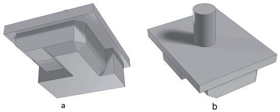
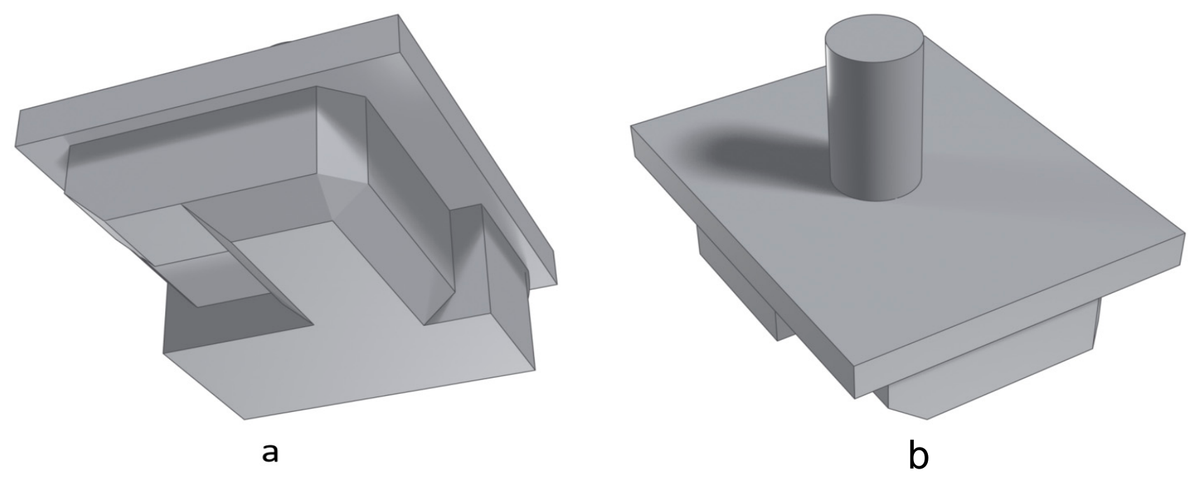
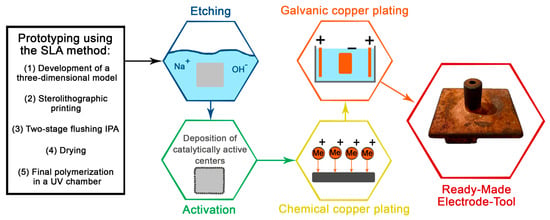
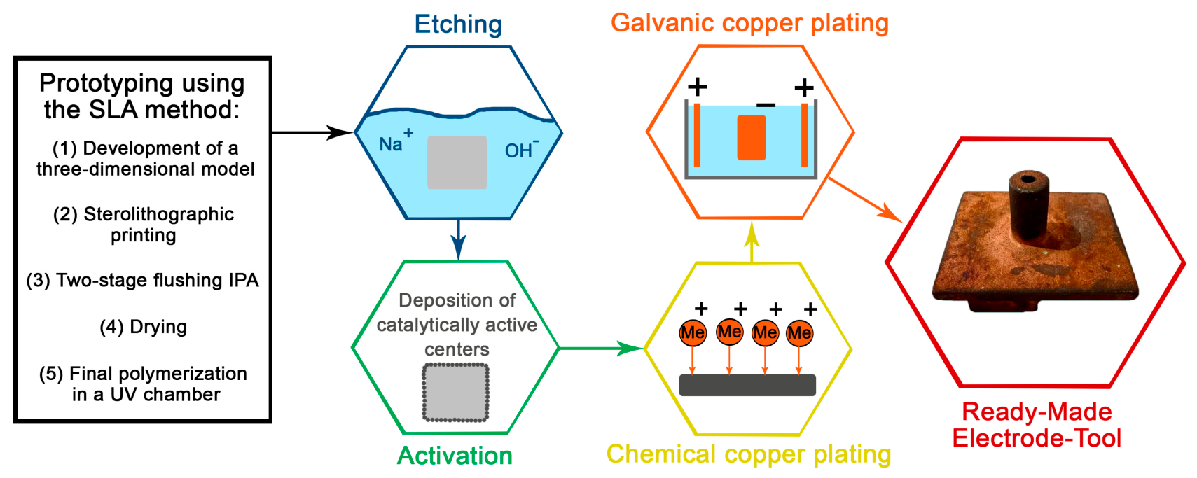
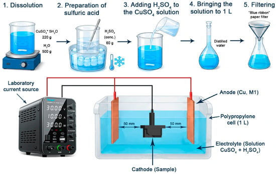
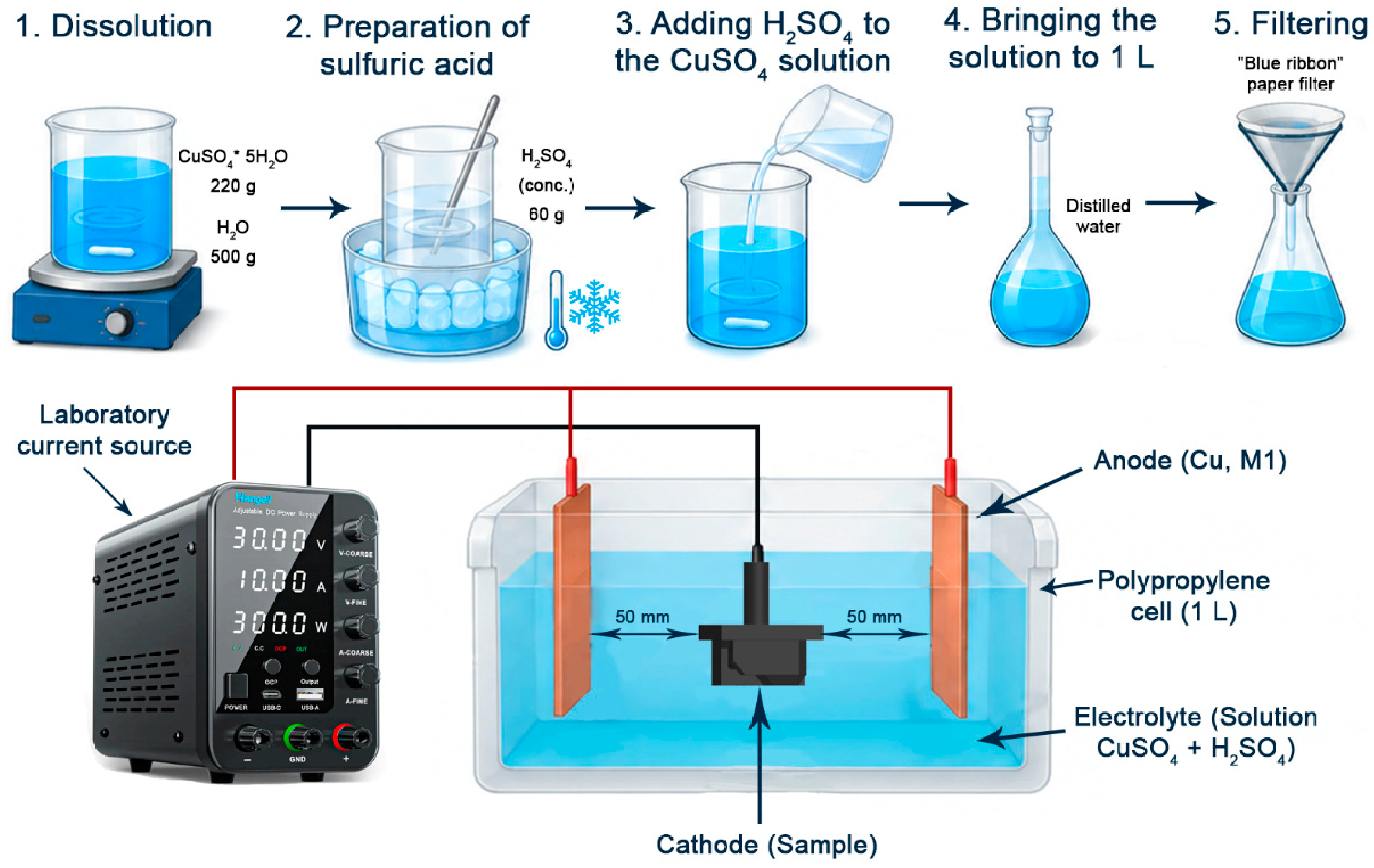
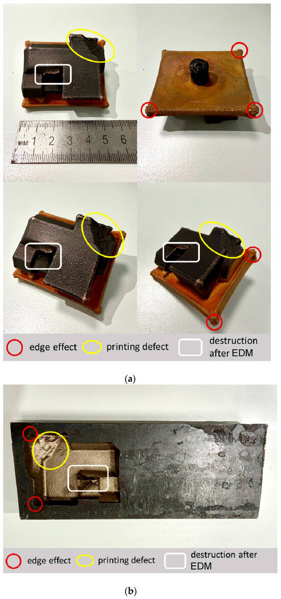
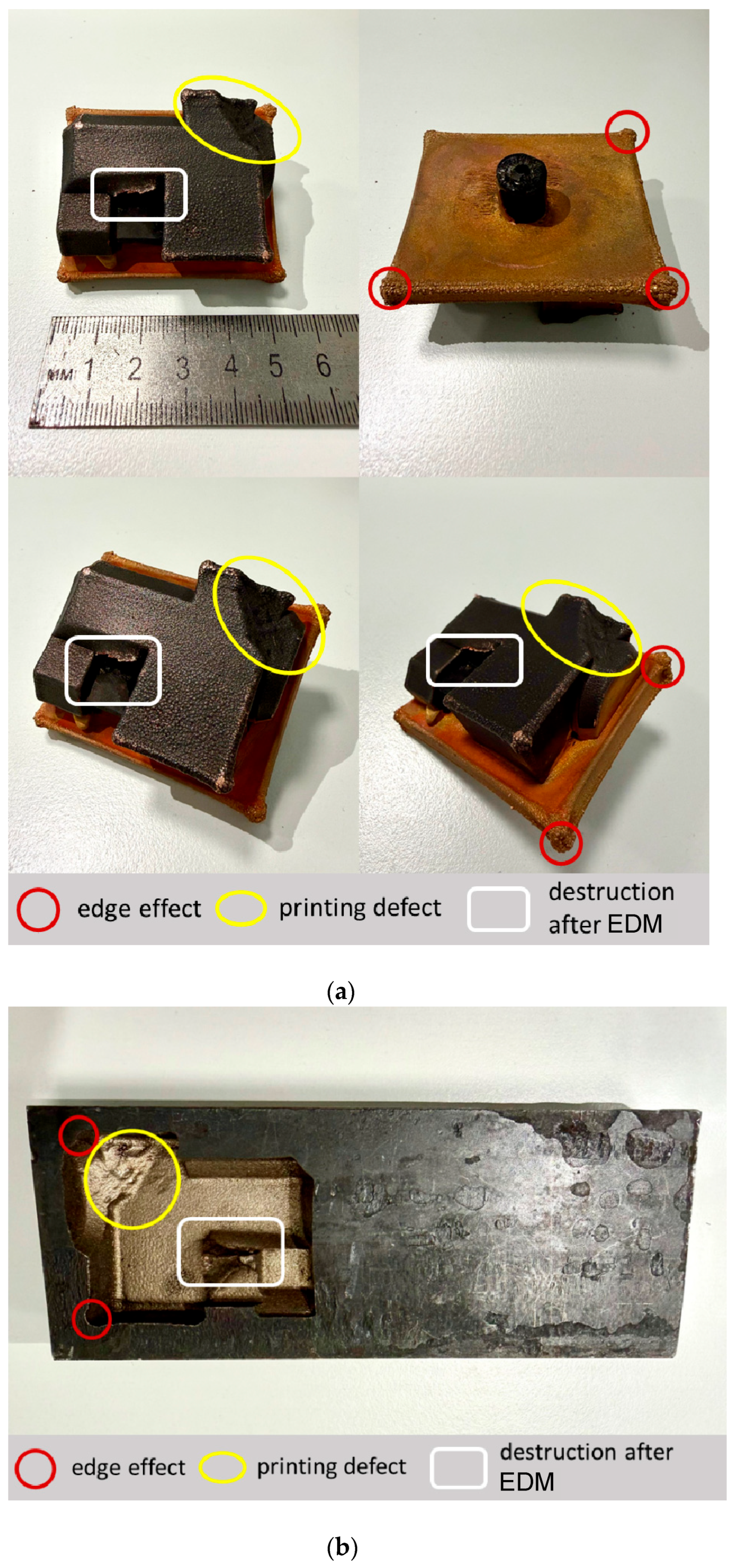
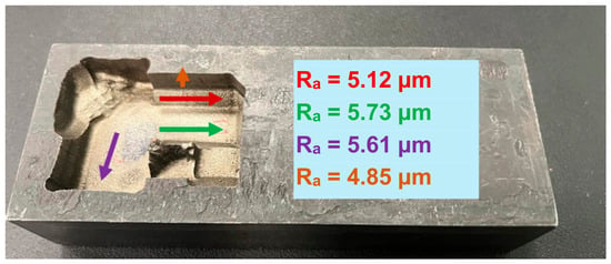
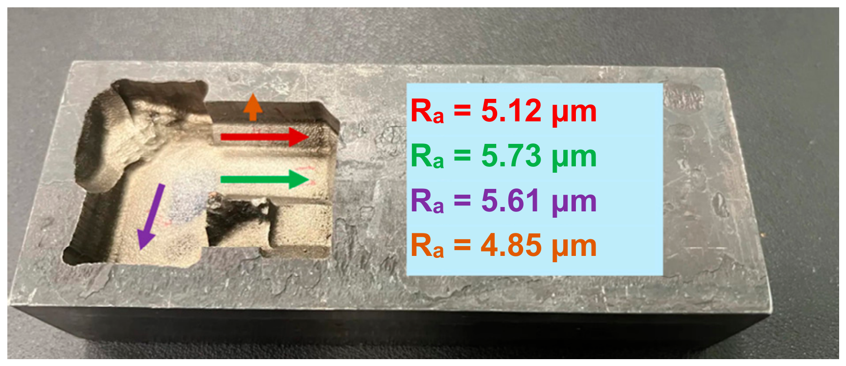
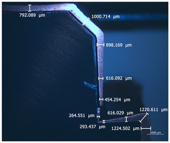
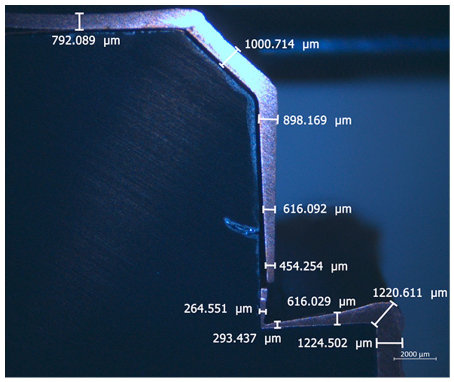
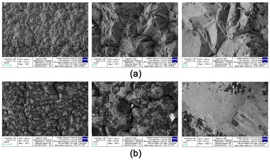
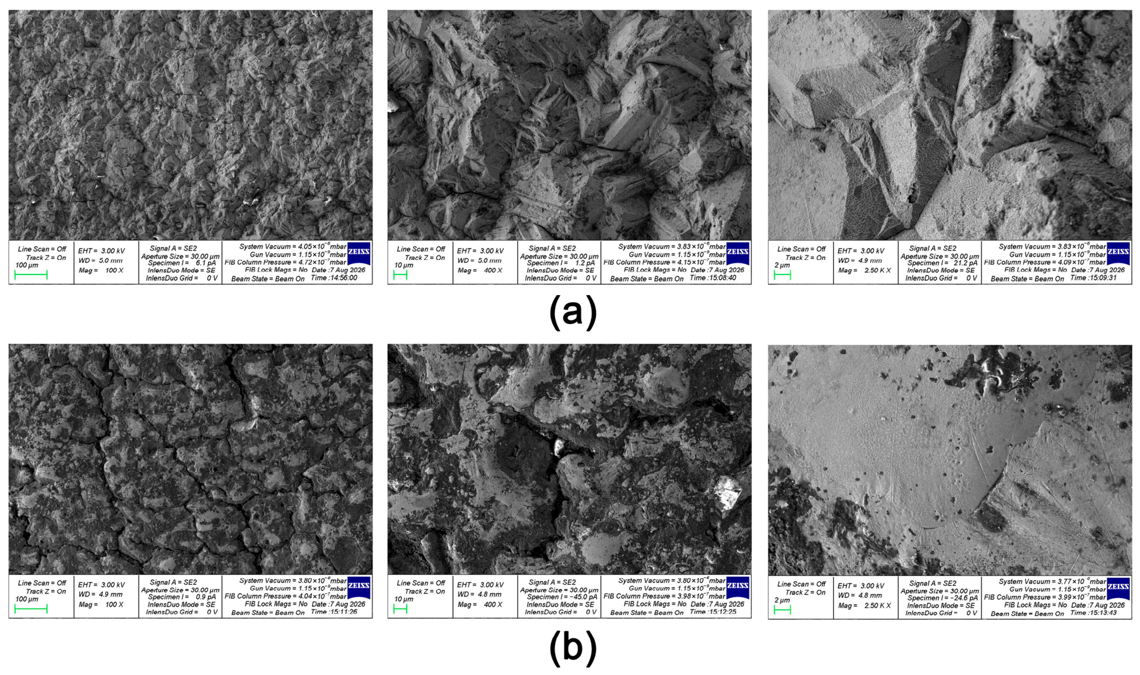
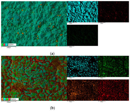
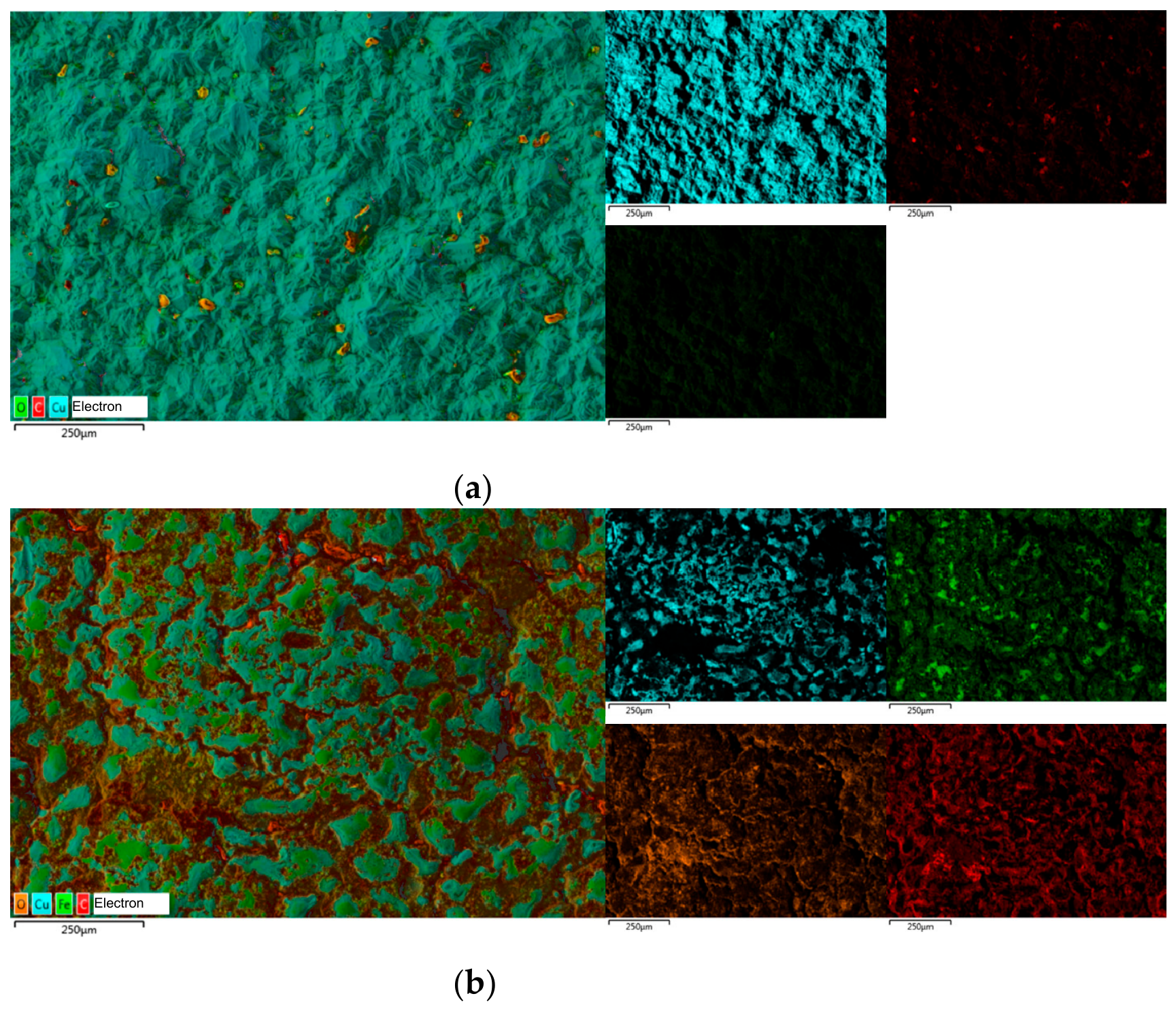
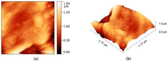
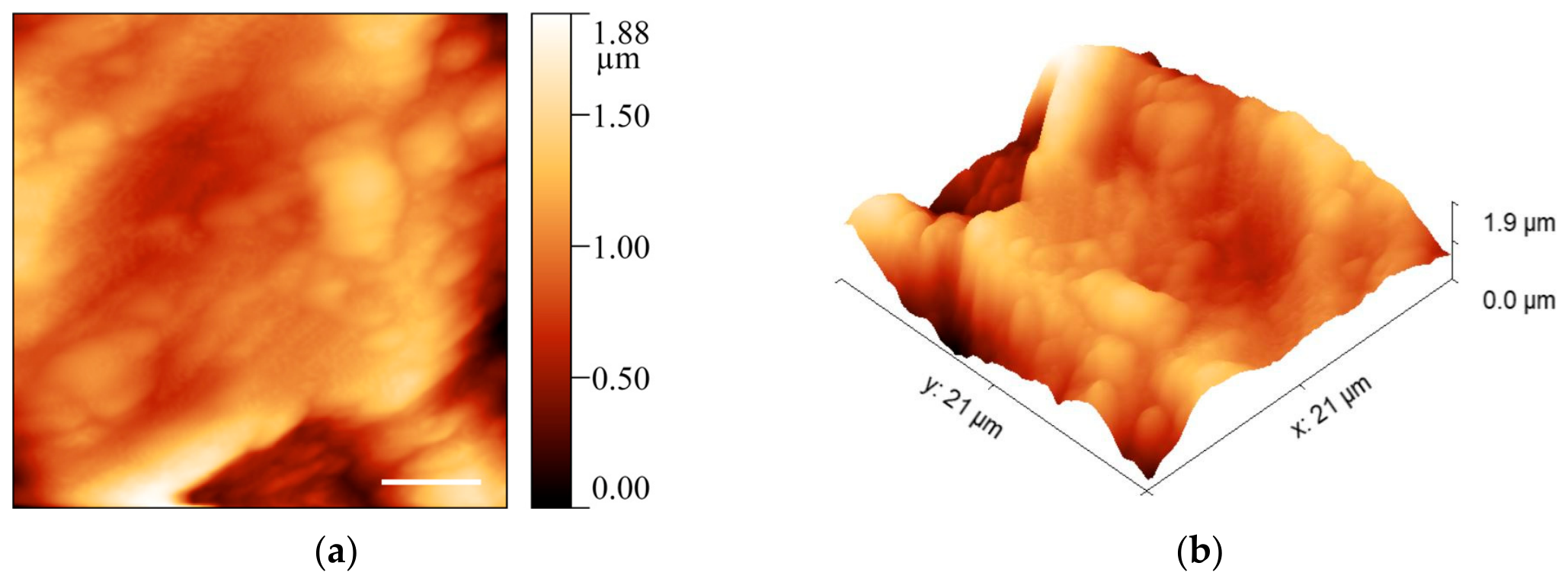
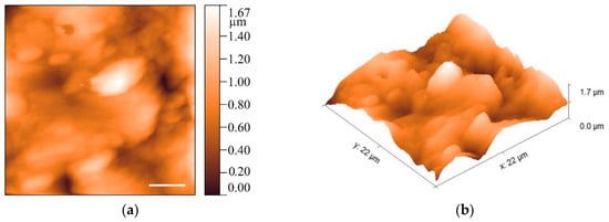
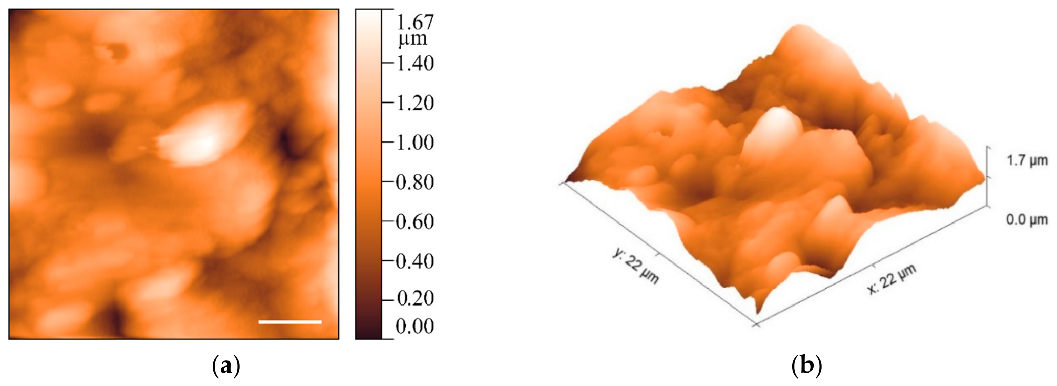
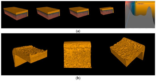
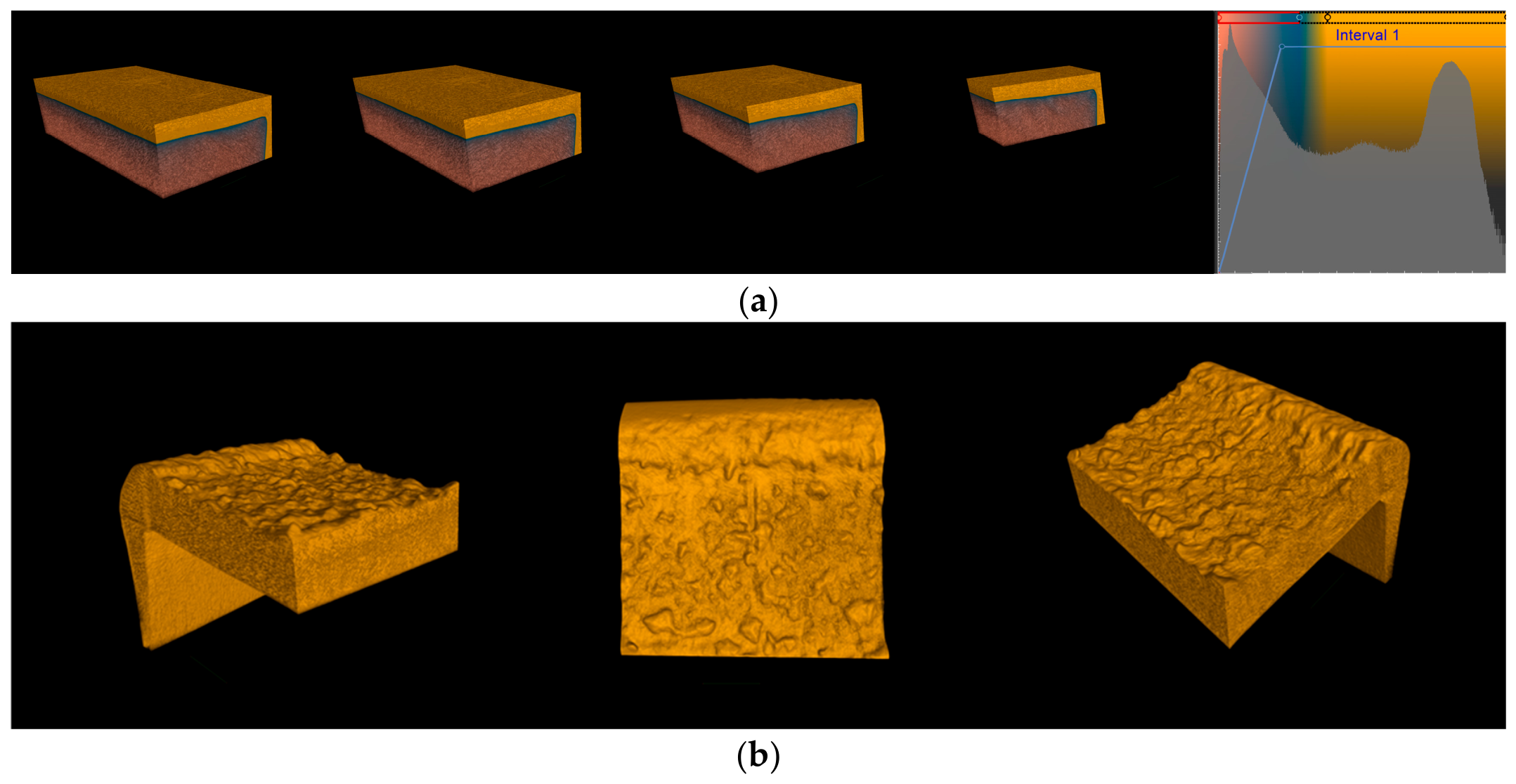
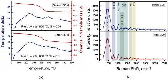
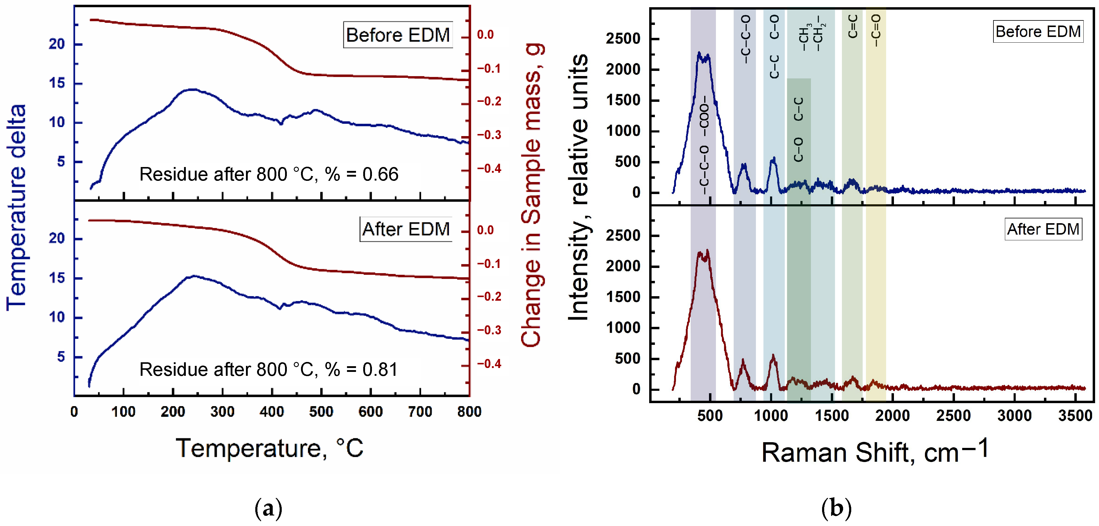
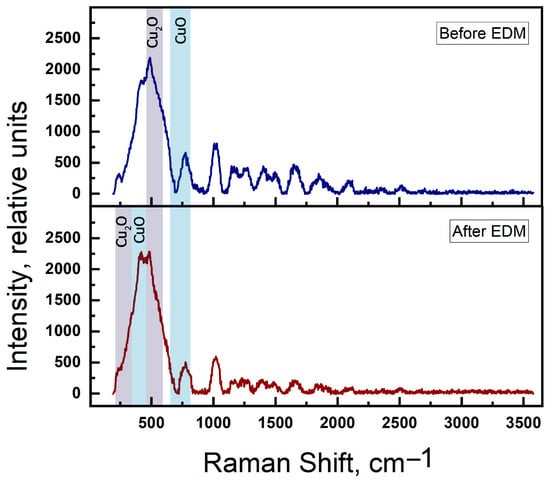
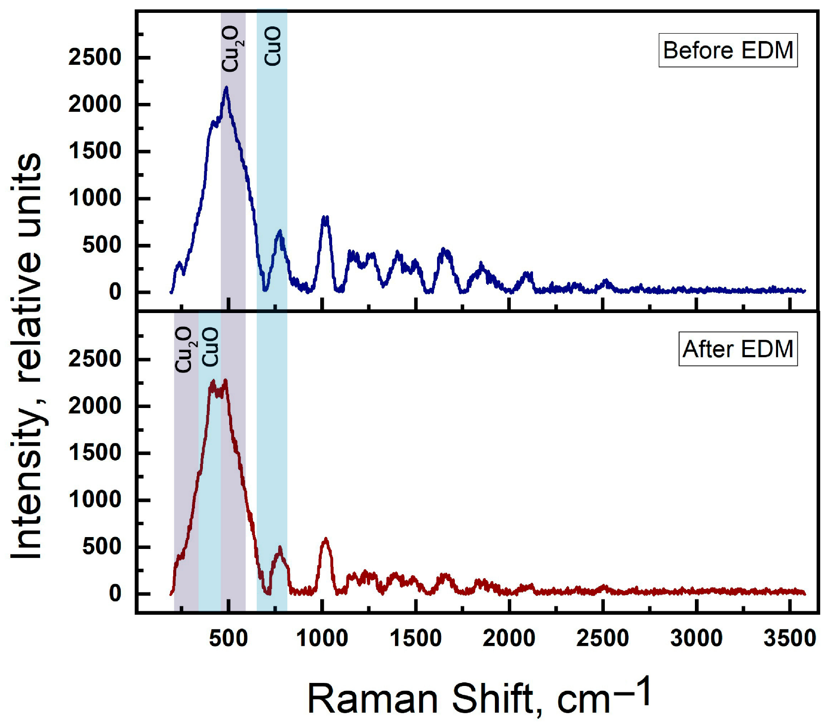
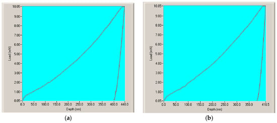
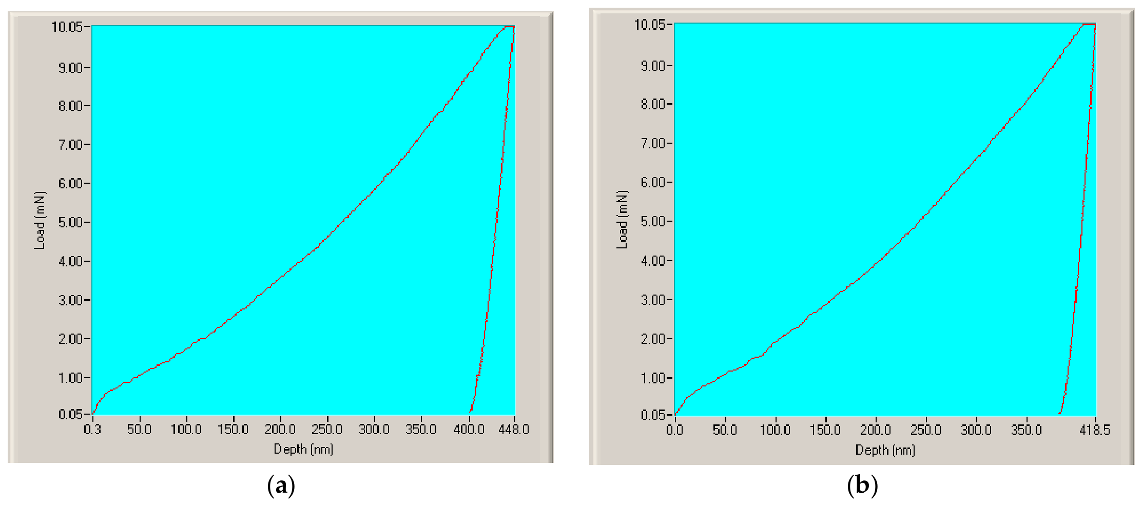
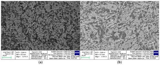
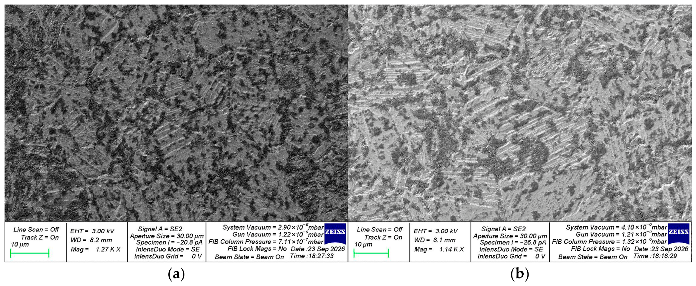
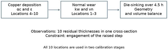
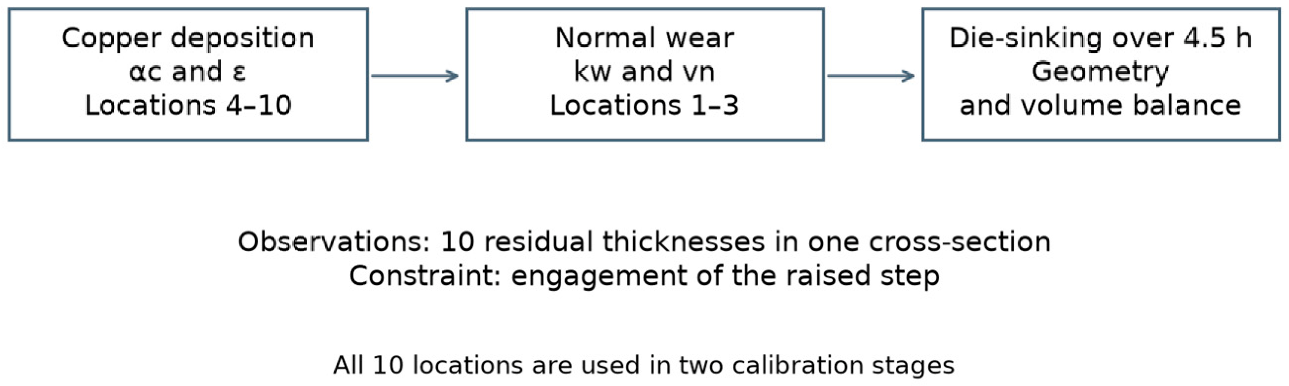
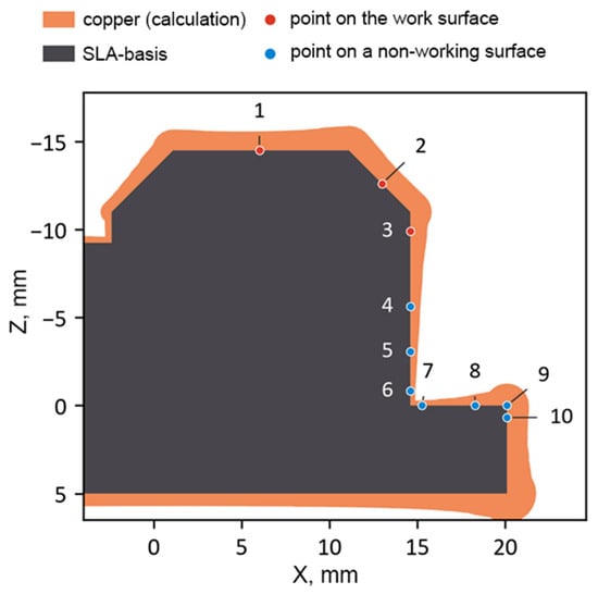
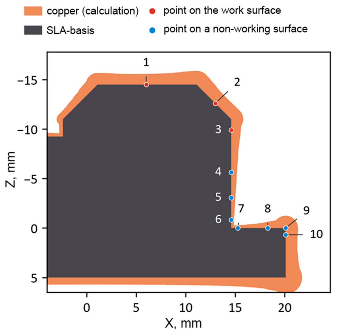
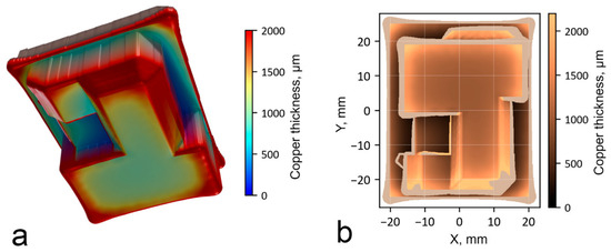
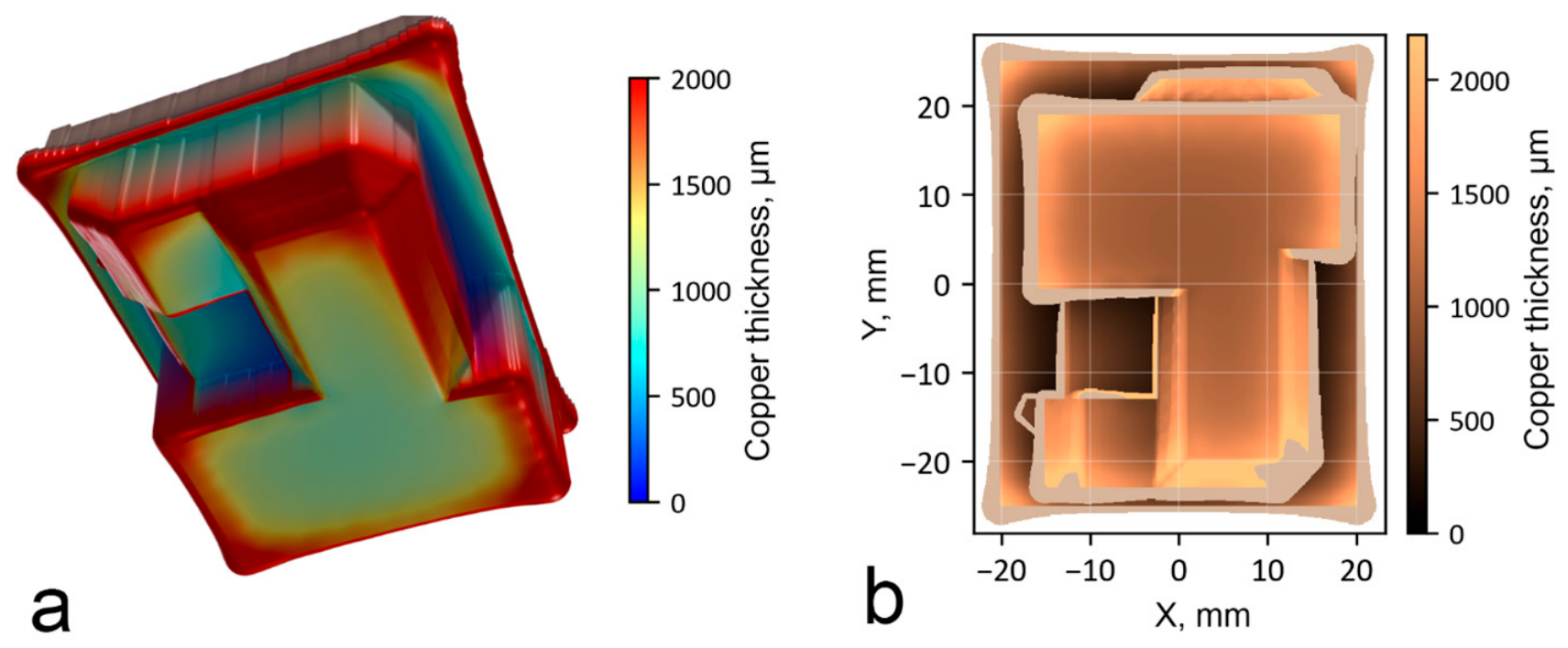
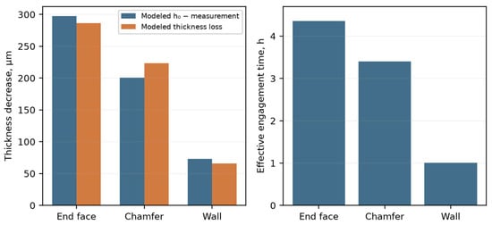
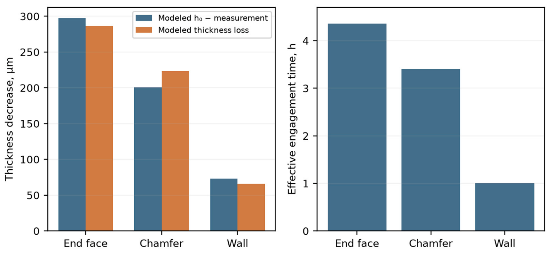
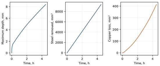
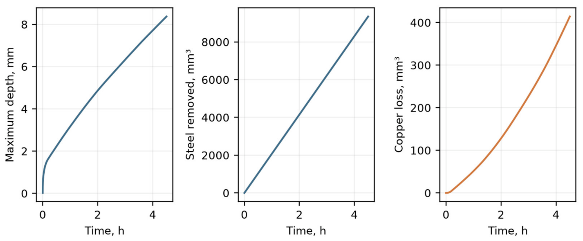
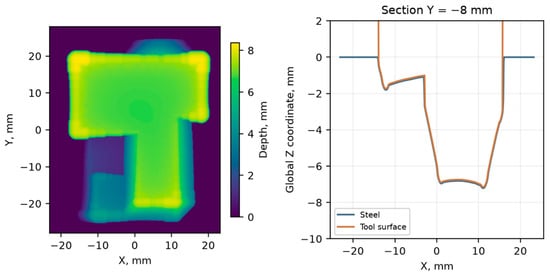
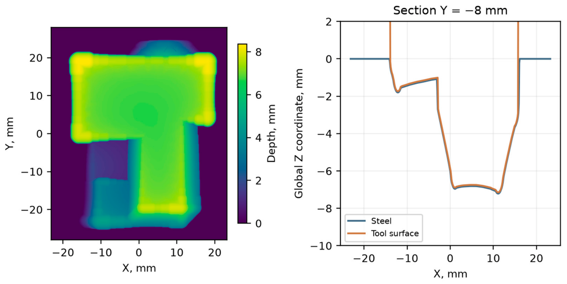
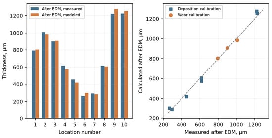
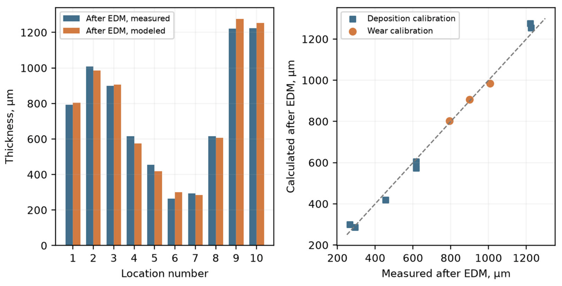
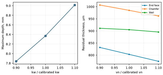
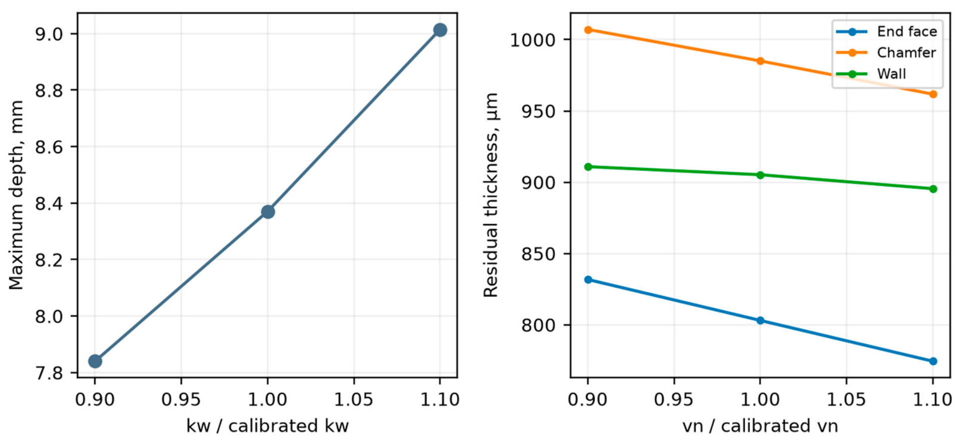

Disclaimer/Publisher’s Note: The statements, opinions and data contained in all publications are solely those of the individual author(s) and contributor(s) and not of MDPI and/or the editor(s). MDPI and/or the editor(s) disclaim responsibility for any injury to people or property resulting from any ideas, methods, instructions or products referred to in the content. |
© 2026 by the authors. Licensee MDPI, Basel, Switzerland. This article is an open access article distributed under the terms and conditions of the Creative Commons Attribution (CC BY) license.