A Learning-Based Measurement Validation Approach for Cooperative Multi-UAV Navigation Using Kalman Filtering

Highlights

What are the main findings?

• A deep learning-based pre-filtering module is integrated into the Kalman filter to detect degraded measurements in a multi-UAV mesh network navigation system.
• The method enhances estimation robustness by evaluating both measurement data and auxiliary reliability metrics before each filter update.

What are the implications of the main findings?

• The integration of AI-driven pre-filtering significantly improves navigation reliability in environments with intermittent or degraded GNSS signals.
• The results demonstrate that intelligent pre-filtering can outperform conventional Kalman filtering approaches in collaborative UAV operations.

Abstract

Reliable navigation in cooperative unmanned aerial vehicle (UAV) networks requires adaptively managing measurement degradations within Kalman-filter-based estimation frameworks. This paper introduces a learning-based Kalman approach for real-time detection of degraded measurements in mesh-network-based multi-UAV navigation. The method incorporates a data-driven pre-filtering module that assesses measurement reliability prior to the Kalman update, thereby improving the robustness of the estimation process under communication-induced degradations. Within this approach, four measurement fault detection strategies—Innovation Filter (IF), Deep Q-Network (DQN), Multi-Layer Perceptron (MLP), and Long Short-Term Memory (LSTM)—were implemented and comparatively evaluated through Monte Carlo simulations combining inertial sensors, time-of-arrival, and Doppler-based inter-agent observations. Additional statistical analyses, including ±1σ error bars and a Wilcoxon rank-sum test, were conducted to verify the significance of the performance differences among the methods. The results show that the proposed approach significantly enhances navigation reliability, particularly under degraded or intermittent GNSS and communication conditions. The MLP-based configuration achieved the best balance between fault-detection accuracy and overall filter consistency. These findings confirm the effectiveness of learning-augmented Kalman filtering architectures for robust and scalable cooperative UAV navigation.

1. Introduction

1.1. Background and Motivation

The Kalman filter has long been a powerful and statistically optimal method for estimating states in linear or approximately linear dynamic systems. It is widely used in navigation and sensor fusion applications, where it provides high estimation accuracy under well-defined system and measurement models with zero-mean Gaussian white noise. In practice, these assumptions are often violated due to model uncertainties and time-varying measurement degradations, both of which can significantly deteriorate filter performance.

This study aims to improve the Kalman filter robustness against measurement-induced disturbances. Instead of relying solely on the Kalman gain to compensate for errors, a deep learning-based pre-filtering module is integrated into the filter structure. Unlike conventional innovation-based gating or statistical thresholding techniques, the proposed approach can identify measurement distortions early and prevent their impact on state estimation. Existing innovation and integrity-monitoring approaches rely on simplified thresholds and cannot fully capture the time-varying or nonlinear behavior of link-induced faults in cooperative UAV navigation. Previous quantitative studies show that such degradations can cause position errors of several meters in GNSS-denied or multipath environments, motivating the need for adaptive, data-driven decision mechanisms.

The system is designed for a cooperative multi-sensor, multi-agent navigation scenario. Each agent performs its own local navigation solution and shares both its estimated state and associated uncertainty information with other agents in the network. Each pair of agents also generates inter-agent range and range-rate measurements through two-way communication. Range measurements are obtained via the time-of-arrival (ToA) method, while range-rate values are derived from Doppler shift analysis. These observations are fused with inertial sensor data to produce a joint navigation solution. However, due to channel distortions and timing synchronization errors in communication-based measurements, the reliability of these observations may degrade, adversely affecting the overall Kalman filter performance.

The proposed learning-based pre-filtering module addresses this issue by analyzing not only the raw measurement values but also additional features that reflect the likelihood and impact of potential measurement errors. This multi-dimensional feature analysis enables the network to detect unreliable measurements before they enter the Kalman update, ensuring that only consistent data are used in the filter. As a result, the Kalman filter receives cleaner input data, achieving higher robustness and improved estimation accuracy.

1.2. Related Works

The Kalman filter, first introduced by R.E. Kalman in 1960 [1], has been extensively applied for optimal state estimation in systems subject to measurement and process uncertainties. Over time, it has become a cornerstone in navigation and sensor fusion frameworks such as GNSS/INS integration. However, the classical approach assumes perfectly known system dynamics and noise characteristics. In practice, these assumptions are rarely valid—model uncertainties, time-varying sensor properties, and measurement degradations often cause substantial performance deterioration. Consequently, the theoretical minimum mean square error (MMSE) optimality of the Kalman filter cannot be achieved under such non-ideal conditions. Recent survey studies also highlight the rise of deep learning-assisted inertial navigation architectures that combine model-based estimation with data-driven adaptation [2].

In integrated navigation systems, where inertial sensors are supported by external signals such as GNSS, the temporary loss or degradation of these signals has become increasingly common. To mitigate this degradation, several neural-network-assisted Kalman filtering techniques have been proposed. Methods employing recurrent or convolutional networks to learn the Kalman gain have shown promising results in nonlinear and time-varying scenarios [3,4]. For instance, KalmanNet [3] achieves near-MMSE performance for linear systems without matrix inversion and provides superior accuracy over conventional Extended or Unscented Kalman Filters in nonlinear cases. Similarly, the CNN-LSTM-based adaptive filter presented in [4] directly estimates the Kalman gain and yields significant performance improvements for GNSS/INS integration. Recent hybrid multi-sensor fusion studies in GNSS-denied environments further highlight the importance of adaptive reliability assessment mechanisms [5].

Several recent studies extend Kalman-type filters toward robust parameter estimation and deep-learning-based adaptation. A robust Extended Kalman Filter for uncertain dynamic systems is proposed in [6] highlighting the benefits of adaptive parameter estimation, while [7] shows that uncertainty modeling plays a critical role in multi-sensor UAV localization.

Other studies reduce the Kalman filter’s sensitivity to measurement noise by learning the measurement model directly. For example, RKFNet [8] predicts measurement-noise statistics using a recurrent network, improving robustness under non-Gaussian conditions. Likewise, refs. [9,10] adaptively adjust the measurement covariance or dynamic model using neural networks to improve estimation accuracy.

A complementary line of research explores post-filter enhancement, where neural or fuzzy models refine Kalman filter outputs. Works such as [11,12,13] demonstrate that hybrid approaches—combining Kalman filtering with Neural Network (NN) or Adaptive Neuro-Fuzzy Inference System (ANFIS) structures—can significantly enhance accuracy. In particular, the ANFIS-KF architecture proposed in [13] has shown substantial performance gains under low-quality GPS. In parallel, several recent contributions have investigated cooperative and multi-UAV navigation filters. Ref. [14] proposed an adaptive fault-tolerant federated Kalman filter for multi-UAV positioning, reporting more than 80% improvement in follower-UAV accuracy relative to single-UAV absolute positioning. Additionally, communication-assisted deep learning frameworks for 5G-enabled UAVs demonstrate robustness under diverse operating conditions [15]. Comprehensive reviews on multi-agent coordination and UAV-based data gathering also emphasize the increasing use of AI-driven fusion and decision making in swarm architectures [16,17].

Some studies employ neural networks as virtual measurement generators to maintain navigation performance during signal outages. For example, NARX or RBF networks have been used to simulate measurement updates in the absence of GNSS signals [18,19]. However, these systems typically activate after complete signal loss and do not include mechanisms for preemptive detection or filtering of degraded measurements.

Additionally, several works have examined integrity monitoring architectures, where the Kalman filter is used to evaluate the consistency between predicted and observed measurements. Classical examples include [20,21,22,23,24,25,26,27], which employ statistical thresholds or solution separation techniques to detect unreliable data. However, these approaches do not leverage deep learning for classification or decision making. More recently, methods such as RAIM-NET [24] apply deep neural networks for GNSS integrity monitoring, yet they are limited to single-sensor configurations and cannot be directly extended to integrated multi-agent systems.

The present study differs from these approaches in several key aspects. First, the proposed Kalman filter operates not only on direct measurements but also incorporates auxiliary reliability indicators. A deep-learning-based pre-filtering module is introduced to detect and reject corrupted or unreliable data before the estimation update. This design enhances both the accuracy and the reliability of the overall navigation solution. Unlike previous AI-augmented Kalman approaches such as KalmanNet or RKFNet, this study introduces a pre-filtering stage applied before the measurement update, enhancing robustness in multi-agent environments. In this way, the proposed method bridges the gap between classical innovation-based gating and recent AI-assisted filters by explicitly targeting the selection and validation of inter-agent measurements in a wireless mesh-network-based multi-UAV navigation scenario.

In addition, neural-network–assisted filtering approaches continue to expand beyond classical architectures; for example, ref. [28] demonstrate a particle-filter–based integrity monitoring framework enhanced by neural network modeling, while ref. [29] introduce a meta-learning–driven KalmanNet variant that adaptively improves filtering performance under varying system dynamics.

Moreover, the method is developed within a collaborative multi-agent framework, where agents exchange both their local state estimates and inter-agent measurements based on time-of-arrival and Doppler-derived range data. This mesh-network-based configuration, previously introduced in [30], enables robust navigation even under degraded external signal conditions. The integration of the proposed pre-filtering module further improves resilience against measurement anomalies, establishing a more reliable cooperative navigation system.

In addition to these developments, several recent studies have explored reinforcement-learning-based cooperative control strategies, which support resilient multi-UAV architectures [31]. Cooperative and learning-based fusion strategies for UAV swarms and real-time fault detection have also been actively investigated in recent literature, further strengthening this trend. Air–ground collaborative navigation work demonstrates the benefits of combining multi-agent information [32], while swarm-based integrated navigation frameworks highlight the value of information sharing [33]. Together, these studies confirm the growing convergence between deep learning and cooperative estimation, underscoring the need for adaptive and fault-tolerant navigation frameworks such as the one presented in this paper.

Deep learning methodologies have also been applied successfully in unrelated domains, demonstrating strong modeling flexibility and temporal prediction capability. Recent examples include biomedical prediction models [34] and hybrid LSTM-based time-series forecasting frameworks [35].

2. Materials and Methods

2.1. Preliminaries

In cooperative UAV navigation, the primary challenge addressed in this study is the degradation of inter-agent range and range-rate measurements caused by communication delays, Doppler-induced distortions, and asynchronous message arrivals. These impairments directly affect the innovation sequence and often violate the Gaussian and consistency assumptions required for reliable Kalman filtering, leading to significant reductions in estimation accuracy. Existing innovation-based gating or thresholding approaches are insufficient under such time-varying fault conditions, because they rely on simplified scalar metrics and cannot capture the nonlinear characteristics of communication-induced errors. Therefore, a more robust, feature-rich, and data-driven measurement validation mechanism is required to ensure reliable state estimation in mesh-networked multi-UAV systems.

The proposed system architecture focuses on achieving sustainable cooperative navigation in environments where GNSS signals are weak, jammed, or unavailable. In this context, the simulation framework was designed to model both the diversity of non-GNSS measurement sources and the degradation scenarios that may affect them.

In this paper, the following notation is adopted. Scalar quantities are denoted using regular lowercase letters (e.g., x), vectors are represented using bold lowercase letters (e.g., x), and matrices are indicated using bold uppercase letters (e.g., P). All vectors are column vectors unless otherwise stated. This notation is used consistently throughout the system model, measurement equations, innovation definitions, and neural-network feature representations.

The multi-agent structure consists of several unmanned aerial vehicles (UAVs) flying cooperatively along predefined trajectories. Each UAV performs coordinated maneuvers at scheduled time intervals to maintain or modify its relative position within the formation. Even in the absence of GNSS signals, the agents generate a joint navigation solution by combining inter-agent communication-based measurements—such as range (Time of Arrival, ToA) and range-rate (Doppler shift)—with their own inertial sensor data.

A learning-based measurement filtering module is integrated into this framework to detect and reject degraded measurements before they enter the Kalman update. This integration ensures that the filter is updated only with reliable data, improving estimation robustness and accuracy.

Details of the simulation setup, algorithmic architecture, network-based measurement framework, error modeling, and training configuration used in this study are presented in the following subsections.

2.1.1. Simulation Environment

Monte Carlo (MC)-based simulations were performed to evaluate the performance of the proposed framework under a variety of stochastic measurement and communication conditions.

All simulations were implemented in MATLAB R2022b and Simulink. The complete multi-UAV navigation model—including sensor, communication, and filtering subsystems—was built in Simulink, while a MATLAB MC controller script called the model for each run. This structure ensured that every algorithm was executed with identical random-seed realizations of sensor and link errors, allowing fair statistical comparison across 256 runs. UAV trajectories and mission geometries were parameterized in MATLAB to allow consistent regeneration for each run.

The Simulink model consisted of modular sensor, communication, and filtering blocks, including a strapdown inertial navigation algorithm, time-of-arrival and Doppler-based inter-agent measurement models, and a Kalman filter augmented with the proposed learning-based decision module. A fixed-step discrete solver with a 30 ms update period was used to match the real-time processing constraints of UAV onboard computers. The IMU, GNSS-denied conditions, and link-impairment models were implemented using parameter sets derived from standard references and manufacturer specifications. This block-structured architecture allowed consistent timing behavior across agents and ensured reproducible evaluation of measurement delays, dropouts, and distortions within the Monte Carlo framework.

A kinematic flight model was developed for fixed-wing unmanned aerial vehicles (UAVs) to evaluate the proposed method. Each UAV represents an agent within a cooperative navigation network. Initially, all agents are positioned in a predefined formation and perform scheduled roll maneuvers to dynamically alter the formation geometry during the simulation.

The model produces reference trajectories containing position, velocity, and attitude data for each UAV. These reference data are generated using the ‘Kinematic_ECEF.m’ function provided in [36], with a sampling interval of 30 ms. The outputs of this function represent the ground-truth reference values and are summarized in Table 1. To ensure consistency and reproducibility, the kinematic and strapdown navigation models employed in this study were implemented using the verified reference codes provided in the appendices of [36]. These components follow established formulations widely adopted in the literature and were used without modification, because they serve primarily as a standardized simulation basis for evaluating the proposed approach.

Table 1. Reference data for each UAV agent.

Data Name	Unit	Description
IMU_Gyr_rad	rad/s	Reference gyroscope measurements
IMU_Acc_mps2	m/s2	Reference accelerometer measurements
Pos_Ecef	m	Earth-Centered Earth-Fixed (ECEF) position vector
Vel_Ecef	m/s	ECEF velocity vector
EulerAngles_rad	rad	Euler angles [Roll, Pitch, Yaw]

Using these reference trajectories, synthetic inertial sensor measurements are generated for each agent. The overall simulation framework is illustrated in Figure 1. In the figure, green-labeled data represent ideal reference values, red-labeled data denote corrupted sensor measurements and estimation outputs, and dashed lines indicate communication between agents. Light-brown-labeled data correspond to inter-agent range and range-rate measurements transmitted via the network. Green arrows indicate error-free reference simulation values, while red arrows represent sensor-corrupted measurements or algorithm outputs. Data transmitted within communication messages are shown using dashed lines.

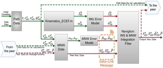
Figure 1. Simulation framework for each UAV agent.

In the adopted notation, the subscript “e” denotes the ECEF frame, “b” represents the body frame of the UAV, and “p” refers to the peer agent with which communication occurs. The subscript “i” indicates the inertial reference frame, assumed to be fixed with respect to distant stars. The vector notation and frame representations adopted in this study are defined below for clarity:

$${\mathit{X}}_{\beta \alpha }^{\gamma }, \mathit{X} \mathsf{ϵ} \left\{r,v,\psi ,f\right\}, \alpha ,\beta \mathsf{ϵ} \left\{i,e,b,p\right\}, \gamma \mathsf{ϵ} \left\{b,e\right\}$$

(1)

where $\mathrm{r}$, $\mathrm{v}$, $\psi$, and $\mathrm{f}$ denote the position, velocity, attitude, and acceleration vectors, respectively. The indices $\alpha$ and $\beta$ represent the reference and target frames, and $\gamma$ indicates the coordinate frame in which the vector is expressed.

The vectors ${\mathbf{r}}_{eb}^e$, ${\mathbf{v}}_{eb}^e$ and ${\mathit{\psi }}_{eb}^e$ represent the position, velocity, and attitude angles of the UAV with respect to the Earth, all expressed in the ECEF reference frame. The variable $t$ denotes time.

The vectors ${\mathbf{f}}_{ib}^b$ and ${\mathit{\omega }}_{ib}^b$ correspond to the specific force and angular rate of the UAV relative to the inertial frame, expressed in the body frame. These quantities represent the ideal reference values expected to be measured by the inertial measurement unit (IMU). The corrupted sensor measurements used in the simulation are denoted by ${\tilde{\mathbf{f}}}_{ib}^b$ and ${\tilde{\mathit{\omega }}}_{ib}^b$, whose error characteristics are defined by the models presented in Equations (2) and (3).

$${\tilde{\mathit{f}}}_{ib}^b={\mathit{b}}_a+\left(\mathit{I}+{\mathit{M}}_a\right){\mathit{f}}_{ib}^b+{\mathit{w}}_a$$

(2)

$${\tilde{\mathit{\omega }}}_{ib}^b={\mathit{b}}_g+\left(\mathit{I}+{\mathit{M}}_g\right){\mathit{\omega }}_{ib}^b+{\mathit{w}}_g$$

(3)

The modeling details are comprehensively presented in [37]. The vector $\mathit{b}$ denotes the constant bias vector, $\mathit{M}$ represents the misalignment matrix and $\mathit{w}$ corresponds to the random walk component of the inertial sensor error model.

When modeling the inertial measurement unit (IMU), the selection of the sensor performance level was made by considering the complexity of the UAV systems addressed in this study, their expected navigation accuracy, mission profiles, and sensor-cost budgets. Accordingly, a tactical-grade or higher IMU was modeled as the most appropriate option. This level allows observable error dynamics while maintaining realistic bias and noise characteristics. A higher-grade IMU was intentionally avoided, since for MC analyses a moderate-quality sensor provides larger stochastic variations and more informative error distributions between runs. The adopted noise and bias characteristics were selected to represent typical tactical-grade IMUs used in UAV navigation, based on literature and manufacturer datasheets (e.g., InertialLab IMU-p, Honeywell HG1700 class), and the corresponding parameter set is summarized in Table 2.

Table 2. IMU error parameters used in the simulation.

Parameter	Description	Value
Gyro bias	Constant bias of the gyro	10°/h
Gyro scale factor	Scale factor error of the gyro	500 ppm
Gyro misalignment	Axis misalignment of the gyro	0.3 mrad
Angular random walk	Noise density of the gyro	0.02°/√h
Accelerometer bias	Constant bias of the accelerometer	1 mg
Accelerometer scale factor	Scale factor error of the accelerometer	100 ppm
Accelerometer misalignment	Axis misalignment of the accelerometer	0.3 mrad
Velocity random walk	Noise density of the accelerometer	100 µg/√Hz

Communication-based computations use the position and velocity vectors of each agent, denoted as ${\mathit{r}}_{eb}^e$ and ${\mathit{v}}_{eb}^e$, together with those of its peer agent ${\mathit{r}}_{ep}^e$ and ${\mathit{v}}_{ep}^e$. Using these quantities, the inter-agent range $\rho$ and range-rate $\dot{\rho }$ reference values are calculated. The measurement error model is applied to generate the corrupted measurements $\tilde{\rho }$ and $\tilde{\dot{\rho }}$.

Through the communication link, each agent also receives its peer’s estimated navigation states, including position (${\widehat{\mathit{r}}}_{ep}^e$), velocity (${\widehat{\mathit{v}}}_{ep}^e$), and the corresponding covariance matrix ($\widehat{P}$), representing the uncertainty of these estimates.

Each agent outputs estimates of its own position, velocity, and attitude, along with the associated covariance matrices. These estimated states are compared with the reference trajectories generated by the simulation to evaluate the accuracy and reliability of the algorithm.

For clarity and reproducibility, the complete modeling procedure used in this study follows a step-wise structure in which each subsystem is explicitly associated with its governing equations. The kinematic and strapdown inertial navigation elements (Equations (1)–(3)) define the motion dynamics and inertial sensor behavior, while the IMU stochastic error components (Table 2, Equations (2) and (3)) specify bias, noise and instability characteristics. The cooperative range and range-rate observations are modeled through the two-way ToA and Doppler equations (Equations (4)–(6)), and the communication-induced degradations are introduced using the stochastic link-fault models in Equations (7)–(9). The INS error-state propagation and its discrete-time formulation (Equations (10)–(14)) define the state prediction step of the Kalman filter, whereas the measurement-update stage relies on the residual definitions, Jacobians, and partial-update mechanisms summarized in Equations (15)–(23). Together, these steps constitute the end-to-end modeling pipeline implemented in the simulation environment and correspond directly to the block-level structure illustrated in Figure 1.

2.1.2. Network-Based Measurement Architecture

The cooperative simulation setup employs a wireless mesh network (WMN) architecture for inter-UAV measurements.

The primary objective of the designed WMN structure is to enable each agent to share its local navigation solution, and the corresponding uncertainty estimates with other agents in the formation. During this exchange, inter-agent range and range-rate information are also communicated over the data link. By leveraging these shared measurements, each UAV can improve its own navigation accuracy based on the geometric configuration of the formation.

Communication among the agents follows a time-division multiple access (TDMA) protocol. As shown in Figure 2, a four-agent network allows six possible pairwise communication combinations. At each time slot, only one agent pair is active, and the active link alternates cyclically according to the TDMA schedule. During an active communication period, both agents exchange their estimated positions and associated uncertainty data. This information is then used to enhance estimation accuracy along the line-of-sight direction between the communicating pair.

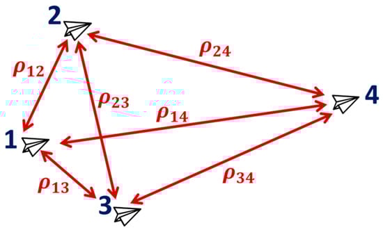
Figure 2. Pairwise communication combinations in a four-agent WMN example.

In an $N$-agent network, the inter-agent range measurement between a pair of communicating agents is modeled as:

$${\rho }_{bp}=‖{\mathit{r}}_{ep}^e-{\mathit{r}}_{eb}^e‖+ {\tilde{\rho }}_{bp}$$

(4)

where ${\mathit{r}}_{ep}^e$ and ${\mathit{r}}_{eb}^e$ denote the ECEF position vectors of the local and peer agents, respectively, and ${\tilde{\rho }}_{bp}$ is a zero-mean Gaussian noise term. In the absence of channel degradation, the standard deviation of ${\tilde{\rho }}_{bp}$ is denoted by $\mathcal{N}\left(0,{{\sigma }_{\rho }}^2\right)$.

Similarly, the inter-agent range-rate measurement is defined as:

$${\overline{\dot{\rho }}}_{bp}={{\mathit{u}}_{bp}^e}^T\left({\mathit{v}}_{ep}^e-{\mathit{v}}_{eb}^e\right)+ {\tilde{\dot{\rho }}}_{bp}$$

(5)

where ${\mathit{v}}_{eb}^e$ and ${\mathit{v}}_{ep}^e$ represent the ECEF velocity vectors of the two agents, and ${\tilde{\dot{\rho }}}_{bp}$ denotes the Gaussian noise associated with the range-rate measurement. The unit line-of-sight vector between the agents is expressed as:

$${\mathit{u}}_{bp}^e= {\displaystyle \frac{{\mathit{r}}_{ep}^e-{\mathit{r}}_{eb}^e}{‖{\mathit{r}}_{ep}^e-{\mathit{r}}_{eb}^e‖}}$$

(6)

In nominal communication conditions, the standard deviation of ${\tilde{\dot{\rho }}}_{bp}$ is denoted by $\mathcal{N}\left(0,{{\sigma }_{\dot{\rho }}}^2\right)$. The degradation behavior of these measurements is captured through dedicated stochastic error models.

2.1.3. WMN Measurement Error Model

In the mesh network configuration, each pair of communicating agents is subject to temporary and systematic measurement degradations that occur randomly over time. A stochastic error model is employed to simulate such degradations for each communication channel. The model checks at every measurement epoch whether a degradation event occurs; if it does, a fixed bias error and a time-varying instability component are introduced and maintained for a randomly determined duration. This structure allows the model to represent both transient and time-dependent error behaviors, as summarized in Equation (7).

$${\tilde{\rho }}_{bp}\left(t\right)=\left\{\begin{array}{cc}b+d\left(t\right)+n_1\left(t\right),& if the channel is degraded,\hfill \\ n_0\left(t\right),& otherwise,\hfill \end{array}\right.$$

(7)

where $b$ is a constant bias term uniformly distributed within $[b_{\mathrm{m}\mathrm{i}\mathrm{n}},b_{\mathrm{m}\mathrm{a}\mathrm{x}}]$. The term $d(t)$ represents a time-varying drift obtained by accumulating small Gaussian perturbations at each sampling step, as defined in Equation (8). $n_0(t)$ and $n_1(t)$ represent the nominal and degraded measurement noises modeled as zero-mean Gaussian processes with variances ${\sigma }_{n_0}^2$ and ${\sigma }_{n_1}^2$, respectively. $\Delta t$ denotes the simulation sampling period.

$$d\left(t\right)={\sum }_{k=1}^{⌊{\displaystyle \frac{t}{\Delta t}}⌋}{\sigma }_d{\xi }_k, {\xi }_k\sim \mathcal{N}(0,1)$$

(8)

The degradation duration $T_f$ is randomly determined as follows:

$$T_f\sim \mathcal{N}\left(T_{min}+\left(T_{max}-T_{min}\right)\cdot \xi \right), \xi \sim \mathcal{N}(0,1)$$

(9)

At each sampling step, the channel transition into the degraded state is governed by a Bernoulli process with probability $p_f$. When a degradation event occurs, the total error added to the measurement consists of the fixed bias, its time-varying instability, and the white-noise component, all acting simultaneously during the degradation period $T_f$. After this period, the channel returns to its nominal state characterized by white noise only, and the same link may subsequently re-enter a degraded state.

This modeling approach allows the simulated measurement data to more accurately reflect the transient error behaviors encountered in real-world conditions, such as communication interference and multipath effects. The overall flow of the error model, which is applied to both range and range-rate measurements, is illustrated in Figure 3, where decision transitions are shown in yellow and error-computation steps are shown in green.

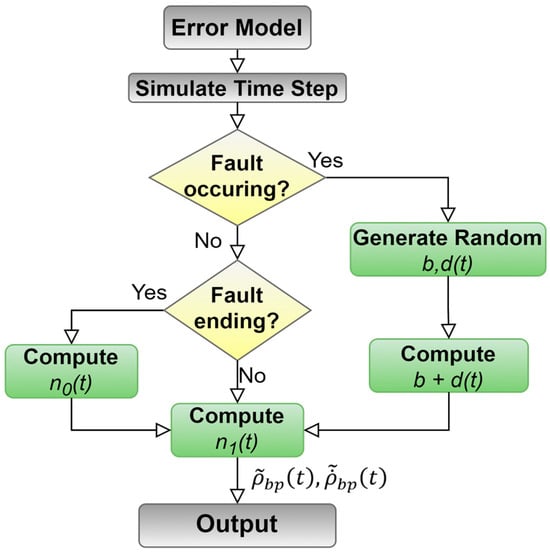
Figure 3. Overall flow of measurement error model.

The parameters used in the error model are summarized in Table 3.

Table 3. Parameters used in the measurement error model.

Parameter	Range Parameters	Range-Rate Parameters
$\mathrm{Fault} \mathrm{occurrence} \mathrm{probability} (p_f$)	0.003	0.003
$\mathrm{Minimum} \mathrm{fault} \mathrm{duration} (T_{min}$)	0.06 s	0.06 s
$\mathrm{Maximum} \mathrm{fault} \mathrm{duration} (T_{max}$)	2 s	2 s
$\mathrm{Minimum} \mathrm{bias} \mathrm{value} (b_{\min }$)	−15 m	−3 m/s
$\mathrm{Maximum} \mathrm{bias} \mathrm{value} (b_{\max }$)	15 m	3 m/s
$\mathrm{Standard} \mathrm{deviation} \mathrm{of} \mathrm{bias} \mathrm{instability} ({\sigma }_d$)	0.1 m/s	0.1 m/s
$\mathrm{Standard} \mathrm{deviation} \mathrm{of} \mathrm{faulted} \mathrm{white} \mathrm{noise} ({\sigma }_{n_1}$)	0.75 m	0.045 m/s
$\mathrm{Standard} \mathrm{deviation} \mathrm{of} \mathrm{nominal} \mathrm{white} \mathrm{noise} ({\sigma }_{n_0}$)	0.25 m	0.025 m/s

2.1.4. Algorithm Framework

The integration of measurements obtained from the mesh network and the outputs of the inertial navigation system (INS) is performed within a linearized Kalman filter framework. The INS error models are defined in the ECEF frame, and all computations are carried out with respect to this reference frame. The filter estimates the error states contained in the error vector defined in Equation (10), which includes three-dimensional vectors representing position, velocity, and attitude errors, as well as the constant accelerometer and gyroscope biases associated with the inertial sensors.

In the simulation, constant biases were identified as the primary error sources significantly affecting the analysis; therefore, only these components were included in the error-state vector. The effects of other error types were represented implicitly through bias instability terms.

This configuration reduces the filter dimension while preserving realism, providing an efficient error model that focuses on the dominant INS error sources.

$${\mathit{X}}_{ANS}^e={\left[\begin{array}{c}\delta {\mathit{r}}_{eb}^e\\ \delta {\mathit{v}}_{eb}^e\\ \delta {\mathit{\psi }}_{eb}^e\\ {\mathit{b}}_a\\ {\mathit{b}}_g\end{array}\right]}_{15\times 1}$$

(10)

where $\delta {\mathbf{r}}_{eb}^e$ represents the position error vector in the ECEF frame, $\delta {\mathbf{v}}_{eb}^e$ denotes the velocity error vector in the same frame and $\delta {\mathit{\psi }}_{eb}^e$ refers to the attitude error vector expressed in Euler angles with respect to the ECEF frame. The vectors ${\mathbf{b}}_a$ and ${\mathbf{b}}_g$ correspond to the constant bias components of the accelerometer and gyroscope, respectively.

The subscript $b$ indicates the body frame of the UAV and takes the values $b=\mathrm{1,2},\dots ,N$ for $N$ agents in the network. These estimated error states are applied in a closed-loop configuration to correct navigation errors in real time.

The state variables defined by the position, velocity, and attitude errors are represented in continuous time by a linearized state-space model as:

$${\dot{\mathit{X}}}_{ANS}^e= {\left[\begin{array}{c}\begin{array}{ccc}{0}_3& \begin{array}{ccc}{I}_3& 0_3& 0_3\end{array}& 0_3\end{array}\\ \begin{array}{ccc}{F}_{21}^e& \begin{array}{ccc}{-2\Omega }_{ie}^e& F_{23}^e& {\widehat{C}}_b^e\end{array}& 0_3\end{array}\\ \begin{array}{ccc}{0}_3& \begin{array}{ccc}{0}_3& {-\Omega }_{ie}^e& 0_3\end{array}& {\widehat{C}}_b^e\end{array}\\ \begin{array}{ccc}{0}_3& \begin{array}{ccc}{0}_3& 0_3& 0_3\end{array}& 0_3\end{array}\\ \begin{array}{ccc}{0}_3& \begin{array}{ccc}{0}_3& 0_3& 0_3\end{array}& 0_3\end{array}\end{array}\right]}_{15\times 1}{X}_{ANS}^e$$

(11)

where ${\Omega }_{ie}^e$ is the skew-symmetric form of the Earth’s rotation vector ${\omega }_{ie}^e$ expressed in the ECEF frame:

$${\mathsf{\Omega }}_{ie}^n=\left[{\mathit{\omega }}_{ie}\right]\mathrm{x}$$

(12)

The term ${\mathrm{F}}_{21}^e$ represents the negative of the skew-symmetric matrix of the accelerometer measurements in the ECEF frame and is defined as:

$${\mathit{F}}_{21}^e=\left[-\left({\widehat{\mathit{C}}}_b^e {\widehat{\mathit{f}}}_{ib}^b\right)\right]\mathrm{x}$$

(13)

The matrix ${\mathrm{F}}_{23}^e$ is expressed as:

$${\mathit{F}}_{23}^e=-{\displaystyle \frac{2{\widehat{\mathit{\gamma }}}_{ib}^e}{{\mathit{r}}_{eS}^e({\widehat{\mathit{L}}}_b)}}{\displaystyle \frac{{{\widehat{\mathit{r}}}_{eb}^e}^T}{\left|{\widehat{\mathit{r}}}_{eb}^e\right|}}$$

(14)

where ${\widehat{\mathit{\gamma }}}_{ib}^e$ denotes the gravity vector computed using the WGS-84 gravity model and expressed in the ECEF frame.

The term ${\mathit{r}}_{eS}^e({\widehat{\mathit{L}}}_b)$ represents the geocentric radius, which varies with the estimated latitude.

The state transition matrix is obtained by linearizing the continuous-time model described above, as detailed in [37], and then discretizing it for numerical implementation.

The system noise covariance matrix is derived following the same procedure.

In the proposed approach, the measurement update step of the Kalman filter is performed exclusively using the available and validated measurements. The range and range-rate observations can be incorporated either jointly or independently. When both measurements are verified as reliable, they are applied simultaneously during the update process. If a degradation is detected in either observation, the filter update is carried out using only the valid measurement. The following formulation describes the update step in the case where only range measurements are utilized.

In the mesh network configuration, the range measurement received from a peer agent is compared with the corresponding predicted value obtained from the nonlinear system model. This comparison yields the measurement residual used in the innovation computation during the Kalman filter update step:

$$z_1={\overline{\rho }}_{bp}-{\widehat{\rho }}_{bp}$$

(15)

The predicted range is defined as:

$${\widehat{\rho }}_{bp}= ‖{\widehat{\mathit{r}}}_{ep}^e-{\widehat{\mathit{r}}}_{eb}^e‖$$

(16)

where ${\bar{\rho }}_{bp}$ denotes the measured range, and ${\widehat{\rho }}_{bp}$ is the predicted range derived from the system model. The vector ${\widehat{\mathbf{r}}}_{eb}^e$ represents the ECEF position estimate of the local agent obtained from the integrated navigation filter, whereas ${\widehat{\mathbf{r}}}_{ep}^e$ is the position estimate of the peer agent received through inter-agent communication. The Euclidean norm of the difference between these two position vectors yields the predicted range. The measurement matrix for the range update is defined as

$${\mathit{H}}_1={\left[\begin{array}{ccccc}{\left({\mathit{I}}_3{\widehat{\mathit{u}}}_{bp}^e\right)}^T& 0_3& 0_3& 0_3& 0_3\end{array}\right]}_{3\times 15}$$

(17)

where ${\widehat{\mathbf{u}}}_{bp}^e$ is the unit line-of-sight vector between the communicating agents expressed in the ECEF frame, computed as

$${\widehat{\mathit{u}}}_{bp}^e={\displaystyle \frac{{\widehat{\mathit{r}}}_{ep}^e-{\widehat{\mathit{r}}}_{eb}^e}{‖{\widehat{\mathit{r}}}_{ep}^e-{\widehat{\mathit{r}}}_{eb}^e‖}}$$

(18)

Range-rate measurements are incorporated into the filter in a similar manner and are used only when their integrity is verified. In this case, the measurement residual is computed as

$$z_2={\overline{\dot{\rho }}}_{bp}-{\widehat{\dot{\rho }}}_{bp}$$

(19)

with the predicted range-rate defined by

$${\widehat{\dot{\rho }}}_{bp}=\left({\widehat{\mathit{v}}}_{ep}^e-{\widehat{\mathit{v}}}_{eb}^e\right) {\widehat{\mathit{u}}}_{bp}^e$$

(20)

where ${\widehat{\mathrm{v}}}_{eb}^e$ and ${\widehat{\mathrm{v}}}_{ep}^e$ denote the estimated velocity vectors of the local and peer agents, respectively. The inner product of their velocity difference with the unit line-of-sight vector provides the predicted range-rate. The measurement matrix for range-rate updates is expressed as

$${\mathit{H}}_2={\left[\begin{array}{ccc}{0}_{1\times 3}& {{\widehat{\mathit{u}}}_{bp}^e}^T& \begin{array}{cc}\begin{array}{cc}{0}_{1\times 3}& 0_{1\times 3}\end{array}& 0_{1\times 3}\end{array}\end{array}\right]}_{1\times 15}$$

(21)

When both range and range-rate measurements are validated simultaneously, the Kalman update step is performed using both observations jointly. In this case, the measurement residual is defined as

$${\mathit{z}}_3={\left[\begin{array}{c}{\overline{\rho }}_{bp}-‖{\widehat{\mathit{r}}}_{ep}^e-{\widehat{\mathit{r}}}_{eb}^e‖\\ {\overline{\dot{\rho }}}_{bp}-\left({\widehat{\mathit{v}}}_{ep}^e-{\widehat{\mathit{v}}}_{eb}^e\right){\widehat{\mathit{u}}}_{bp}^e\end{array}\right]}_{2\times 1}$$

(22)

and the combined measurement matrix becomes

$${\mathit{H}}_3={\left[\begin{array}{c}\begin{array}{ccc}{{\widehat{\mathit{u}}}_{bp}^e}^T& 0_{1\times 3}& 0_{1\times 9}\end{array}\\ \begin{array}{ccc}{0}_{1\times 3}& {{\widehat{\mathit{u}}}_{bp}^e}^T& 0_{1\times 9}\end{array}\end{array}\right]}_{2\times 15}$$

(23)

The decision table for the measurement update modes is presented in Table 4.

Table 4. Measurement update modes.

${\overline{\dot{\mathit{\rho }}}}_{\mathit{b}\mathit{p}}$ Valid	${\overline{\mathit{\rho }}}_{\mathit{b}\mathit{p}}$ Valid	Update Mode	$\mathbf{H},\mathbf{z}$	Description
0	0	0	N/A	No measurement update; prediction only
0	1	1	${\mathit{H}}_1,z_1$	Range-only measurement update
1	0	2	${\mathit{H}}_2,z_2$	Range-rate-only measurement update
1	1	3	${\mathit{H}}_3,{\mathit{z}}_3$	Combined range and range-rate update

Several mechanisms are implemented to dynamically manage the measurement update mode when faults occur, preventing degraded observations from adversely affecting the filter performance.

The following model is used to represent the uncertainty associated with the range measurements:

$$R_1= {{\sigma }_{\rho }}^2+{\left(\begin{array}{c}{\widehat{\mathit{P}}}_{peer}(\mathrm{1,1})\\ {\widehat{\mathit{P}}}_{peer}(\mathrm{2,2})\\ {\widehat{\mathit{P}}}_{peer}(\mathrm{3,3})\end{array}\right)}^2·\left({{\widehat{\mathit{u}}}_{bp}^e}^2\right)$$

(24)

where ${\widehat{\mathit{P}}}_{\mathrm{peer}}(i,i)$ (for $i=\mathrm{1,2},3$) represents the first three diagonal elements of the covariance matrix associated with the peer agent’s position estimates. The scalar product of these terms with the unit line-of-sight vector ${\widehat{\mathbf{u}}}_{bp}^e$ quantifies the position-estimate uncertainty along the communication direction. The term ${\sigma }_{\rho }^2$ denotes the measurement noise variance, previously defined in Equation (5).

A similar uncertainty model is applied for the range-rate measurements, with the measurement covariance term defined as

$$R_2={{\sigma }_{\dot{\rho }}}^2+{\left(\begin{array}{c}{\widehat{\mathit{P}}}_{peer}(\mathrm{4,4})\\ {\widehat{\mathit{P}}}_{peer}(\mathrm{5,5})\\ {\widehat{\mathit{P}}}_{peer}(\mathrm{6,6})\end{array}\right)}^2·\left({{\widehat{\mathit{u}}}_{bp}^e}^2\right)$$

(25)

This formulation follows the same principle as the range-based model, directly reflecting the estimation uncertainty along the measurement direction and thereby improving the overall filter performance.

When both measurements are available and validated, the two covariance values are combined into a diagonal matrix $R_3$:

$${\mathit{R}}_3= \left[\begin{array}{cc}{R}_1& 0\\ 0& R_2\end{array}\right]$$

(26)

This configuration integrates both range and range-rate measurement uncertainties into the filter, enhancing update consistency by accounting for estimation uncertainty along the measurement direction.

The Kalman filter is implemented with a closed-loop feedback structure, which dynamically evaluates uncertainty along the measurement direction to ensure more consistent updates. Further methodological details are provided in [36].

2.1.5. Simulation Scenario

In the simulation environment, a scenario was designed to enable a fair comparison of the navigation performance of different methods. In this setup, a formation of four UAVs initially performs a coordinated flight in a predefined configuration. At the start of the simulation ($t=0 \mathrm{s}$), one of the UAVs in the formation releases a separate high-speed UAV, which accelerates approximately 45 km forward to execute an assigned mission.

The total simulation duration is set to 130 s. During this period, the remaining UAVs in the formation perform coordinated roll maneuvers, turning alternately to the right and left. This behavior creates a more favorable geometric distribution that enhances the navigation accuracy of the high-speed UAV. A top-down view of the formation and the flight trajectories of all agents are illustrated in Figure 4. This scenario provides a dynamic and application-oriented test environment for evaluating data-sharing-based enhancement processes within the mesh network architecture.

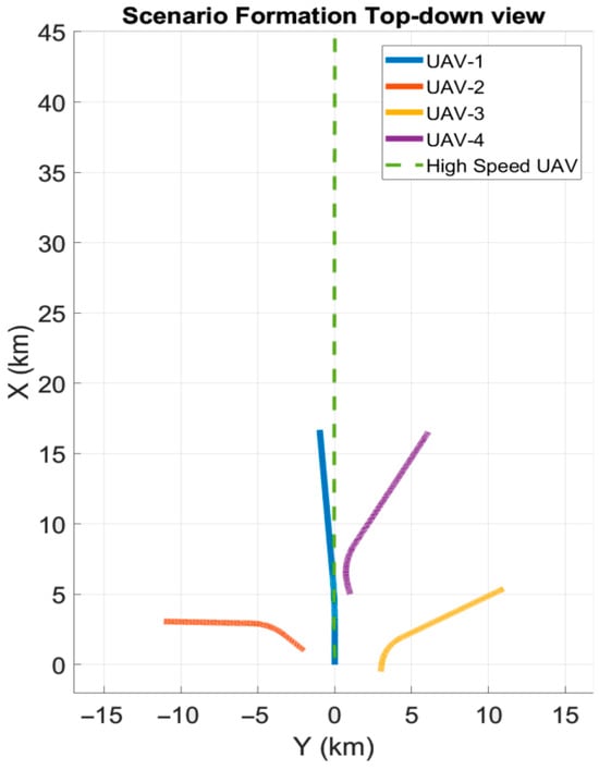
Figure 4. Top-down view of the simulation scenario.

Within this scenario, Monte Carlo (MC) simulations were conducted in which both inertial sensor and communication errors varied stochastically. To ensure a fair comparison among different measurement-mode selection strategies, a mechanism was implemented that generated all random variables identically across runs based on their execution index. This configuration ensured that, although the individual error realizations differed between runs, all methods were evaluated under identical stochastic conditions, maintaining consistency across simulations.

Due to the randomness of the inertial sensor errors, the formation geometry shown in Figure 4 exhibited slight variations between runs within a predefined tolerance range. At the beginning of each run, the inertial sensor error parameters specific to that trial were randomly drawn from zero-mean normal distributions and kept constant throughout the simulation. The standard deviations of these distributions were determined based on the nominal error values provided in Table 2, ensuring a statistically consistent and controlled error model.

Under this configuration, 256 MC runs were performed for each method. For the high-speed UAV, position, velocity, and attitude errors were recorded, along with the algorithmic decisions regarding the measurement update mode and the corresponding communication degradations. This allowed direct observation of each algorithm’s decision accuracy and its influence on navigation performance under identical simulation conditions.

2.1.6. Training Dataset Configuration

To enable the deep learning-based algorithms to make accurate decisions regarding the presence of measurement faults, suitable input parameters were defined for both the algorithm and the simulation environment. In particular, for reinforcement learning (RL)-based architectures, several indirect features were introduced as additional inputs to allow the algorithm to learn the direct impact of potential measurement faults on navigation performance based on the current state. This configuration was designed to improve the decision accuracy and effectiveness of the developed models in achieving the intended outputs. The list of the 29 input parameters selected as features for the network is presented in Table 5.

Table 5. Selected input features for the deep neural network.

Input Feature	Dimension	Description
Time	1	Flight time
Innov	2	Kalman innovation [range; range rate]
InnovCov	2	Kalman innovation covariance [range; range rate]
InnovNorm	2	Kalman innovation norm [range; range rate]
Range	1	Range measurement
RangeRate	1	Range rate measurement
DOP	4	Dilution of precision [norm; x; y; z]
Cov	6	State prediction covariance [3 position; 3 velocity]
EulerAngle	3	Attitude angles
UnitVector	3	Direction of the communication unit vector
MacOneHot	4	One-hot vector for active MAC slot, indicating current communication assignment

The 29-dimensional feature vector was selected after a series of ablation experiments conducted during network development. Early prototypes that used only raw range and range-rate measurements achieved poor discrimination performance, especially under intermittent link errors and Doppler-induced disturbances. Features related to innovation statistics, covariance-weighted residuals, and Doppler consistency proved essential—removing either group caused the MLP validation accuracy to drop by 10–15%. Additional tests confirmed that reducing the feature set below 20 elements consistently degraded classification accuracy, particularly in scenarios with asynchronous message arrivals or rapidly varying relative geometries. Because the decision mechanism is instantaneous rather than temporal, the network requires a sufficiently rich snapshot of the current measurement and its reliability indicators. The resulting 29-feature configuration provided the most reliable balance between representational richness and computational efficiency.

The last four input features, represented by the “MacOneHot” vector, were introduced to prevent LSTM- or CNN-based deep learning models from incorrectly capturing sequential patterns in the TDMA-based communication structure. Such models are capable of learning temporal dependencies; however, the periodic but alternating nature of the TDMA pattern may lead to false correlations. These features indicate which peer the high-speed UAV is communicating with at the current time step. Instead of a numerical (1–4) encoding, a separate bit is assigned to each agent through one-hot encoding, allowing the time-series models to make more accurate predictions without being affected by systematic biases arising from the communication sequence.

A Monte Carlo simulation consisting of 1024 runs was conducted to generate label data corresponding to communication degradations along with the selected input features. A different random number generator library was used for this simulation compared to that employed in the algorithm testing phase. This ensured statistical independence between the training and test datasets. In addition, a subset of 10 randomly selected runs from the training data was reserved as the validation set.

To assess the quality of the generated dataset, a correlation matrix was computed for all input features, and analyses were carried out based on this matrix. These analyses revealed linear relationships among features and allowed the identification of redundant or multicollinear inputs that could potentially affect model performance.

Although relatively high linear correlations were observed among some input parameters, these relationships were not found to have any significant adverse effect on the training process or the generalization capability of the model. To preserve feature diversity and to exploit potential nonlinear dependencies, all parameters were retained in the training phase without any feature elimination. The correlation matrix is illustrated in Appendix A and Figure A1.

2.2. Methods

Several algorithms are introduced to determine which measurements can be used while preserving Kalman filter performance under degraded conditions. Each algorithm is described in terms of how it adaptively manages the measurement update process and is evaluated with respect to its influence on overall navigation performance.

The algorithms—Innovation Filter (IF), Deep Q-Network (DQN), Multi-Layer Perceptron (MLP), and Long Short-Term Memory (LSTM)—were implemented in MATLAB/Simulink and executed on a standard workstation. Preliminary timing tests showed that the framework operates faster than real time, indicating that the proposed architecture does not impose significant computational demand. Additional implementation and hardware details are provided in Appendix B.

2.2.1. Innovation Filter (IF)

In conventional Kalman filter implementations, the Innovation Filter is frequently employed to assess measurement inconsistencies. As a reference approach, a threshold-based innovation algorithm was first examined. The inputs used in this approach include the innovation, its covariance, and the innovation norm—features also utilized by the other algorithms, as listed in Table 5.

The innovation vector is calculated as:

$$\mathit{y}={\mathit{z}}_3- {\mathit{H}}_3\widehat{\mathit{X}}$$

(27)

The innovation is computed using both measurement components; however, during the Kalman update, only the parts corresponding to valid measurements are applied depending on the algorithmic decision.

Unlike scalar gating methods that compress multidimensional residuals into a single threshold value, the proposed vectorized innovation norm preserves component-wise information associated with range and range-rate measurements. This distinction is essential because the objective of the proposed approach is not only to reject severely corrupted observations but also to exploit partially valid measurement components whenever possible. For example, in cases where the range measurement is degraded while the Doppler-based range-rate remains reliable, using a scalar innovation norm would force both components to be discarded simultaneously. By evaluating the full innovation vector, the system can selectively retain the undistorted components, enabling partial measurement updates as defined in Table 4. This allows the learning-based module to capture subtle inconsistencies across different measurement channels and ensures that useful information is not lost due to localized faults. Similarly, the innovation covariance is given by

$$\mathit{S}={\mathit{H}}_3\widehat{\mathit{P}}{{\mathit{H}}_3}^T+{\mathit{R}}_3$$

(28)

and the vectorized innovation norm used to evaluate the reliability of each measurement component is defined as:

$${\mathit{y}}^{norm}={\displaystyle \frac{\mathit{y}}{\sqrt{diag(\mathit{S})}}}$$

(29)

Since the vectorized innovation norm is normalized component-wise, it allows each measurement element to be assessed individually in proportion to its own reliability, in addition to the commonly used scalar innovation norm. The absolute value of each component is compared against a predefined threshold to evaluate the consistency of the corresponding measurement.

A scalar innovation norm was not considered as a baseline because it compresses all residual components into a single value and is therefore incompatible with the partial-update mechanism summarized in Table 4, which requires preserving component-level innovation information.

The resulting consistency information is used as an input to the decision logic summarized in Table 4, determining the measurement update mode applied in the Kalman filter.

An ablation study was conducted to evaluate the sensitivity of the Innovation Filter to the choice of innovation-norm threshold. Sixteen threshold values between 1 and 5.5 were tested, and the resulting detection accuracy curve is shown in Figure 5. The results indicate that thresholds below 4 are overly aggressive, causing unnecessary rejection of partially valid measurements and reducing overall accuracy due to decreased measurement utilization (increased false positives). Conversely, thresholds above 4 become too permissive, allowing a larger fraction of degraded observations to pass through the update step (increased false negatives), which in turn deteriorates navigation consistency. The threshold value of 4 provided the best balance between rejecting corrupted measurements and retaining reliable components, and was therefore selected as the nominal operating point for all experiments. The threshold value was set to 4 in the MC simulations.

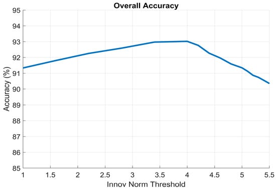
Figure 5. Innovation filter accuracy as a function of the innovation-norm threshold.

2.2.2. Reinforcement Learning (RL)

The simulation environment was configured so that the RL agent could observe the consequences of its decisions and receive rewards or penalties accordingly. The reward and penalty mechanism were defined based on the changes in navigation errors during simulation time steps where a WMN update occurred. If the position and velocity errors decreased after an update, a reward was given to the agent; conversely, an increase in these errors resulted in a penalty.

To prevent the RL agent from favoring a single type of update (e.g., only range or only range-rate), an additional bonus reward was introduced when both measurements were used simultaneously (measurement mode 3) and the reward condition was satisfied.

The total reward applied at each step consisted of two main components: a position-accuracy-based term ($r_p$) and a velocity-accuracy-based term ($r_v$), defined as follows:

$${\mathfrak{r}}_p= \tanh (‖{\mathit{r}}_{ep}^e(t)-{\widehat{\mathit{r}}}_{eb}^e(t)‖-‖{\mathit{r}}_{ep}^e(t-∆t)-{\widehat{\mathit{r}}}_{eb}^e(t-∆t)‖)$$

(30)

$${\mathfrak{r}}_v=\tanh (‖{\mathit{v}}_{ep}^e(t)-{\widehat{\mathit{v}}}_{eb}^e(t)‖-‖{\mathit{v}}_{ep}^e(t-∆t)-{\widehat{\mathit{v}}}_{eb}^e(t-∆t)‖)$$

(31)

The position- and velocity-based components, together with the bonus reward applied when the measurement mode equals three ($m=3$), are combined to yield the total reward value at each time step:

$$\mathfrak{r}=\left\{\begin{array}{cc}0.4 {\mathfrak{r}}_p+0.6 {\mathfrak{r}}_v+{\mathfrak{r}}_{bonus},& if m=3 \wedge {\mathfrak{r}}_p>0 \wedge {\mathfrak{r}}_v>0\\ 0.4 {\mathfrak{r}}_p+0.6 {\mathfrak{r}}_v, & otherwise \end{array}\right.$$

(32)

where $r_{\mathrm{bonus}}=0.5$.

The network input features listed in Table 5 were used as the observable states for the RL agent. Training was conducted by continuously varying the stochastic parameters in the simulation environment, ensuring a generalizable learning process distinct from the test dataset used in the MC simulations.

A Deep Q-Network (DQN)-based reinforcement learning agent was employed. The DQN structure is appropriate for this problem because it processes continuous feature vectors while operating over a discrete action space. The learning process was further stabilized through mechanisms such as the target network and experience replay buffer. For these reasons, the DQN agent was evaluated as an effective and suitable approach for the measurement selection problem. The architecture designed for the DQN agent is illustrated in Figure 6.

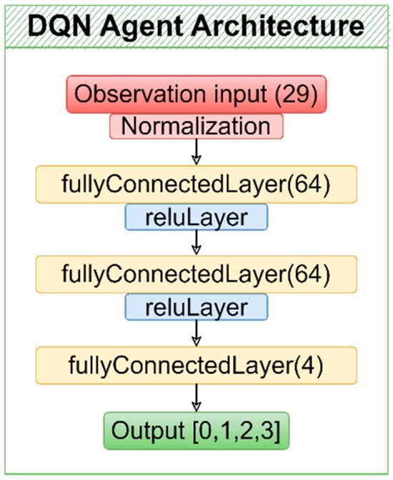
Figure 6. DQN agent network architecture.

During training, multiple hyperparameter variations—including changes in exploration rates, reward coefficients, discount factors, and target-network update frequency—were tested to stabilize convergence and improve decision consistency. Although certain configurations yielded smoother training trajectories, the overall learning performance remained constrained by the limited temporal structure imposed by the TDMA-based measurement sequence, which prevented the DQN agent from reliably exploiting long-term dependencies. The final parameter set reported in Appendix C and Table A2 represents the most stable and consistent configuration obtained.

2.2.3. Multi-Layer Perceptron (MLP)

Multi-layer perceptrons are widely used neural-network models due to their capability to learn nonlinear decision boundaries, making them suitable for classification problems. An MLP-based structure was designed to make decisions solely from instantaneous observation data, without considering the temporal continuity of measurement errors. The designed network was trained to determine the appropriate measurement update mode, and its performance was evaluated through MC simulations after the training process was completed.

Training experiments demonstrated that network stability was highly sensitive to learning rate and mini-batch selection. High learning rates (1 × 10⁻³ to 5 × 10⁻⁴) converged quickly but consistently yielded lower validation accuracy (≈0.86), whereas reducing the learning rate to 1 × 10⁻⁵ and increasing the batch size improved generalization. Furthermore, the application of z-score normalization and class-balanced weighting significantly improved classification robustness, increasing validation accuracy to nearly 0.97. The final training configuration summarized in Table A3 reflects the most stable and generalizable setup identified after extensive experimentation with multiple architectural and hyperparameter combinations.

Several MLP architectures were evaluated during development, including both shallow (64-32-4) and deeper networks (64-64-16-4). Increasing network depth or width did not improve validation accuracy beyond approximately 0.86 and often introduced mild overfitting, especially in the presence of class imbalance. Conversely, smaller networks lacked sufficient capacity and produced unstable gating decisions. The best balance between accuracy, robustness, and computational efficiency was achieved with a compact 3-layer architecture (64-32-4) trained using z-score normalization and class-balanced weights, which increased validation accuracy to nearly 0.97. This architecture also provided the lowest inference latency, making it suitable for real-time deployment in resource-constrained UAV platforms.

The chosen architecture of the proposed MLP model is illustrated in Figure 7. The optimized network parameters, which yielded the best training performance for the MLP, are summarized in Appendix C and Table A3.

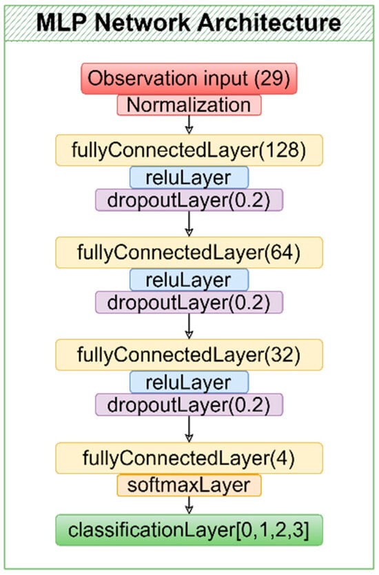
Figure 7. MLP network architecture.

2.2.4. Long-Short Term Memory (LSTM)

LSTM networks, known for their ability to learn temporal dependencies, provide effective solutions for capturing sequential patterns in time-series data. To account for the temporal continuity of measurement degradations, an LSTM-based architecture was developed. The objective was to enable the selection of the measurement update mode based not only on the instantaneous state but also on the temporal patterns observed in previous time steps, thereby achieving more consistent decision making. The architecture of the proposed LSTM model is illustrated in Figure 8.

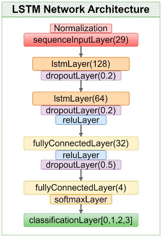
Figure 8. LSTM network architecture.

Several architectural and training variations were tested during model development, including different hidden-layer sizes, dropout configurations, minibatch settings, and class-weight adjustments. Although class-weighted models improved validation accuracy (reaching values above 95%), the limited temporal structure imposed by the TDMA-based measurement sequence prevented the LSTM from fully exploiting its long-term memory capability, ultimately constraining its decision-making performance compared to the MLP. The optimized network parameters, which yielded the best training performance for the LSTM, are summarized in Appendix C and Table A3.

3. Results

Following the Monte Carlo simulations conducted using different methods, confusion matrices, the temporal variation of estimation errors for each run, and the combined RMS error plots for all runs were analyzed.

For quantitative evaluation, root-mean-square (RMS) errors were selected as the primary performance metric because they provide a statistically meaningful measure of the average estimation deviation over the full Monte Carlo ensemble and are widely used in navigation performance assessment. RMS values capture both bias and dispersion effects and reflect cumulative degradation caused by intermittent or time-varying measurement faults, making them particularly suitable for the mesh-network-based cooperative scenario examined in this study. In addition, the innovation norm was chosen as the reference metric for fault characterization because it directly quantifies the discrepancy between predicted and observed measurements and is the most sensitive indicator of communication-induced distortions in Kalman-based fusion frameworks. These metrics together provide a comprehensive and interpretable measure of how measurement faults propagate through the estimation process.

3.1. Innovation Filter Results

The confusion matrix obtained from the results of the Innovation Filter is presented in Figure 9.

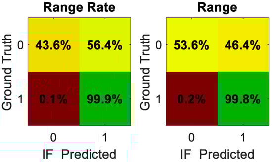
Figure 9. Confusion matrix for IF-based decisions.

According to the confusion matrix, the algorithm achieved high accuracy in cases where no measurement faults were present. However, under faulty conditions, the correct detection rates were observed as 53.6% for range measurements and 43.6% for range-rate measurements. Under these conditions, the temporal variations of the navigation errors for the 256-run simulation set are illustrated in Figure 10.

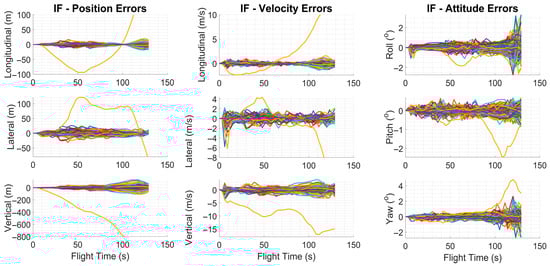
Figure 10. Navigation errors for 256 Monte Carlo runs using the IF method.

In one of the 256 Monte Carlo runs, it was observed that a fault occurring at a critical moment could not be detected, leading to a degradation in navigation performance for the remainder of the flight. This run was treated as an outlier and excluded from the RMS error calculation. The RMS error and uncertainty estimates are presented in Figure 11.

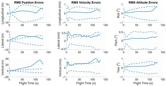
Figure 11. RMS errors and ±1σ uncertainty estimates (dashed lines) for the IF method.

Examination of the RMS error variation over time for the vertical position component revealed that the error exceeded the predicted uncertainty bounds by a significant margin.

This behavior is attributed to the low detection rate of measurement faults, which limits the filter’s ability to correct accumulated errors.

3.2. Reinforcement Learning Results

The confusion matrix of the measurement fault detection decisions predicted by the DQN agent for the 256-run simulation set is presented in Figure 12. In cases where measurement faults occurred, the correct detection rates were 19.9% for range measurements and 12.2% for range-rate measurements.

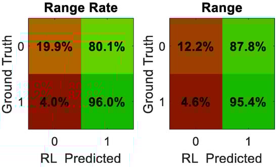
Figure 12. Confusion matrix for RL-based decisions.

Under conditions where measurement faults were detected with very low accuracy, the temporal variations of the navigation errors for the 256-run simulation set are illustrated in Figure 13.

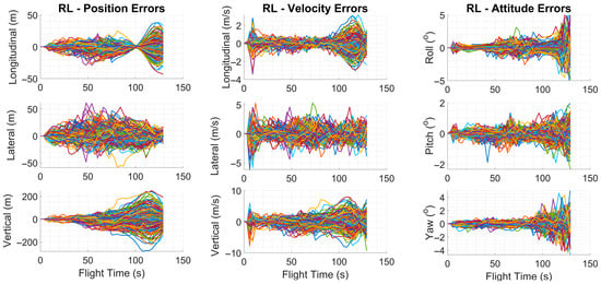
Figure 13. Navigation errors for 256 Monte Carlo runs using the RL method.

In the MC simulations where the measurement update mode was determined by the DQN agent, the distribution of navigation errors was noticeably broader compared to that obtained with the Innovation Filter.

Although no clear outliers were detected, the run with the highest error magnitude was treated as an outlier to ensure a fair comparison and was excluded from the RMS error calculations presented in Figure 14.

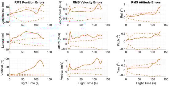
Figure 14. RMS errors and ±1σ uncertainty estimates (dashed lines) for the RL method.

Similar to the previous case, the low fault-detection rate resulted in RMS errors exceeding the predicted uncertainty bounds for this method as well.

3.3. Multi-Layer Perceptron Results

The confusion matrix of the measurement fault detection decisions predicted by the MLP network for the 256-run simulation set is presented in Figure 15.

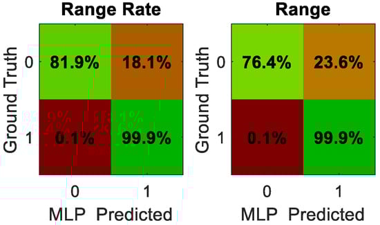
Figure 15. Confusion matrix for MLP-based decisions.

For fault-free measurements, the correct decision rate reached 99.9% for both range and range-rate observations. Under faulty measurement conditions, the correct detection rates were 81.9% for range measurements and 76.4% for range-rate measurements. The temporal variations of navigation errors for the 256-run simulation set obtained using the MLP method are illustrated in Figure 16.

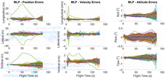
Figure 16. Navigation errors for 256 Monte Carlo runs using the MLP method.

In the MC simulations where the measurement update mode was determined by the MLP network, an improvement in the error distributions was observed compared to the Innovation Filter results. One run identified as a potential outlier was excluded from the analysis and not considered in the RMS error calculations.

As shown in Figure 17, the higher fault-detection rates resulted in lower RMS values compared to the other methods. In addition, the uncertainty bounds were generally maintained, with only the vertical position error component slightly exceeding these limits.

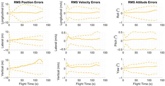
Figure 17. RMS errors and ±1σ uncertainty estimates (dashed lines) for the MLP method.

3.4. Long Short-Term Memory Results

The confusion matrix of the measurement fault detection decisions predicted by the LSTM network for the 256-run simulation set is presented in Figure 18.

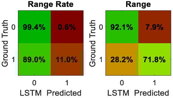
Figure 18. Confusion matrix for LSTM-based decisions.

Although the detection of range faults was achieved with high accuracy, the rate of fault-free measurements incorrectly classified as faulty was considerable. For range-rate measurements, the LSTM network tended to classify most measurements as faulty, indicating a relatively higher false alarm rate.

The temporal variations of the navigation errors for the 256-run simulation set obtained using the LSTM method are illustrated in Figure 19.

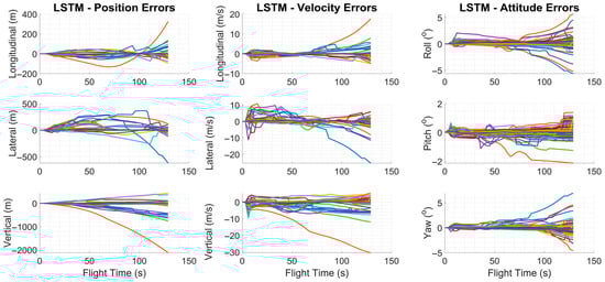
Figure 19. Navigation errors for 256 Monte Carlo runs using the LSTM method.

Because the algorithm tended to classify most measurements as faulty, measurement updates occurred only rarely, which prevented the correction of accumulated inertial errors.

The calculated RMS errors are presented in Figure 20. Because the frequency of measurement updates was much lower compared to the other methods, the estimated uncertainty bounds were observed to be significantly wider.

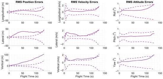
Figure 20. RMS errors and ±1σ uncertainty estimates (dashed lines) for the LSTM method.

3.5. Statistical Evaluation

To assess the statistical reliability of the Monte Carlo (MC) results, algorithm performance was evaluated using descriptive metrics and non-parametric significance tests. For each run, the RMS errors of position, velocity, and attitude were recorded, and their means and standard deviations were used to form the ±1σ uncertainty representations shown in Figure 11, Figure 14, Figure 17 and Figure 20. Vertical error-bar plots were additionally included to more explicitly illustrate dispersion across MC runs. For clarity, the algorithms were grouped into two figures—IF and MLP (Figure 21), and RL and LSTM (Figure 22)—to avoid overlapping uncertainty intervals and to allow clearer within-group comparison.

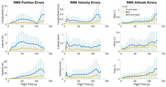
Figure 21. RMS errors with vertical ±1σ error bars for the IF and MLP methods.

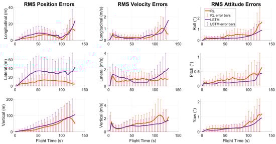
Figure 22. RMS errors with vertical ±1σ error bars for the RL and LSTM.

These visualizations indicate the dispersion of results across 256 MC runs and illustrate the consistency of each algorithm under stochastic conditions. To verify whether the observed performance differences among algorithms were statistically meaningful, a Wilcoxon rank-sum test was applied to the per-run RMS error distributions. This non-parametric test is suitable for data that may not follow a normal distribution and evaluates whether two samples originate from populations with equal medians.

The test was applied pairwise across all algorithms (IF-RL, IF-MLP, IF-LSTM, RL-MLP, RL-LSTM, and MLP-LSTM) using RMS position, velocity, and attitude errors. The resulting p-values remained below 0.05 for all comparisons, indicating that the performance differences among algorithms are statistically significant rather than being caused by random variations in the MC simulations. The summarized outcomes of these pairwise Wilcoxon tests are presented in Table 6, providing the corresponding p-values for all algorithm combinations.

Table 6. Wilcoxon rank-sum test results for pairwise algorithm comparisons based on RMS error distributions.

Comparison	RMS Position	RMS Velocity	RMS Attitude
IF-RL	p ≈ 2 × 10−48	p ≈ 6 × 10−71	p ≈ 5 × 10−66
IF-MLP	p ≈ 2 × 10−62	p ≈ 1 × 10−73	p ≈ 2 × 10−41
IF-LSTM	p ≈ 4 × 10−25	p ≈ 2 × 10−8	p ≈ 4 × 10−8
RL-MLP	p ≈ 3 × 10−83	p ≈ 4 × 10−84	p ≈ 4 × 10−84
RL-LSTM	p ≈ 3 × 10−59	p ≈ 3 × 10−54	p ≈ 8 × 10−60
MLP-LSTM	p ≈ 7 × 10−17	p ≈ 4 × 10−40	p ≈ 1 × 10−12

Overall, this statistical evaluation framework combines the visualization of ±1σ uncertainty with non-parametric significance testing to ensure a consistent and transparent interpretation of the algorithm-comparison results.

4. Discussion

This study aimed to develop navigation solutions resilient to measurement degradations in a cooperative scenario involving multiple UAVs communicating within a mesh network architecture. For this purpose, four different methods were evaluated for measurement fault detection: the conventional Innovation Filter (IF), a reinforcement learning-based DQN agent (RL), a Multi-Layer Perceptron (MLP), and a time-dependent Long Short-Term Memory (LSTM) network.

The LSTM network exhibited lower performance because the TDMA-based communication structure prevented the formation of consistent temporal patterns. Although the MAC index was included as a discrete input to help distinguish temporal sequences for each agent, this addition did not lead to a meaningful improvement in the LSTM’s performance.

The inferior performance of the LSTM network can be attributed to the fact that the measurement-reliability decision is inherently instantaneous rather than sequential. Because TDMA-based communication produces sparse and nonuniform temporal patterns, the recurrent structure cannot exploit long-term temporal dependencies, causing the LSTM to converge on suboptimal representations. In contrast, the MLP effectively learns the nonlinear mapping between innovation features, Doppler-based indicators, and local consistency metrics without assuming temporal continuity, which explains its more stable and accurate classification performance.

The RL agent, which learned from the results of previous decisions, also struggled to assess certain situations accurately and failed to achieve the expected level of stability due to its relatively low false-negative rates.

In contrast, the MLP network, despite relying solely on instantaneous observation data, achieved higher accuracy and consistency in fault detection compared to the IF method. The MLP improved the detection rate of range faults by 23% and range-rate faults by 38% relative to the IF approach. This improvement is statistically significant and reflects a clear gain in overall navigation performance.

Beyond its higher accuracy, the MLP demonstrated superior robustness due to its ability to exploit the expanded 29-dimensional feature vector, which includes innovation statistics, covariance-weighted residuals, Doppler consistency indicators, and geometric attributes of inter-agent links. Unlike the IF method, which relies solely on scalar innovation thresholds, the MLP jointly evaluates multiple reliability cues, enabling more consistent decisions under rapidly varying link conditions. This multi-feature representation enhances sensitivity to subtle distortions while maintaining very low false-negative rates, directly contributing to the observed reduction in position, velocity, and attitude RMS errors.

The overall impact of each method on navigation performance was evaluated using the RMS errors computed from the Monte Carlo runs, and the comparative results are presented in Figure 23.

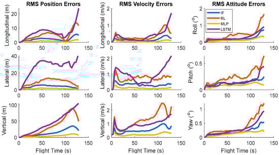
Figure 23. Comparison of RMS error values for different methods.

While the proposed vectorized innovation norm provided improved sensitivity to multidimensional measurement inconsistencies during pre-filtering, its performance advantage was problem-specific rather than universal. Simulation results showed that its effectiveness was particularly strong in scenarios dominated by Doppler-induced distortions and asynchronous message arrivals, whereas in low-dynamics conditions the improvement over scalar norms was more modest. Therefore, the method should be regarded as broadly applicable but not universally optimal for all navigation configurations.

The RMS navigation errors obtained from the Monte Carlo analyses are presented in Table 7 in a ranked order for different algorithms.

Table 7. RMS error values for different algorithms.

	Position Error (m) *			Velocity Error (m/s) *			Attitude Error (°)
	X	Y	Z	X	Y	Z	Roll	Pitch	Yaw
MLP	2	1	7	0.1	0.1	0.3	0.3	0.1	0.2
IF	5	2	21	0.2	0.4	0.8	0.7	0.2	0.5
RL	12	5	50	0.5	0.9	2.3	1.7	0.6	1.2
LSTM	24	43	105	1.7	2.2	1.7	0.9	0.4	0.9

* X: longitudinal, Y: lateral, Z: vertical.

Non-parametric pairwise significance tests (Wilcoxon rank-sum) confirmed that all algorithms exhibited statistically distinct RMS performance distributions (p < 0.05) after FDR (False Discovery Rate) correction. The MLP-based method achieved the lowest RMS errors, significantly outperforming IF, RL, and LSTM across all metrics (Table 6).

Future research will address the characterization and mitigation of data link-induced errors, aiming to fine-tune the pre-filtering mechanism and retrain the learning models using real-world communication data and implementation environments.

Although the MLP achieved the best performance among the evaluated methods, several precautions were taken to avoid overfitting. The network was trained using z-score normalization, class-balanced weighting, and mini-batch regularization, and its learning curve exhibited closely aligned training and validation loss trajectories. Moreover, the statistically significant performance differences observed in the Monte Carlo simulations indicate that the MLP’s improvement stems from better generalization rather than memorization.

Despite its promising performance, the proposed approach has several limitations. First, the simulations were conducted under a controlled formation scenario with a fixed number of UAVs; therefore, scalability to larger swarms or fully decentralized architectures requires further investigation. Second, the communication channel impairments were modeled statistically, and real-world interference patterns such as multi-path fading, clock drift, or burst packet losses may introduce additional challenges. Third, although the MLP is computationally lightweight, its reliability still depends on the representativeness of the training data, and performance may degrade under unseen fault modes. These aspects highlight the need for broader testing and potential architectural extensions.

5. Conclusions

This study presented a comprehensive evaluation of real-time detection and management of measurement faults in mesh network-based multi-UAV navigation systems. The developed and tested methods clearly demonstrated the influence of measurement reliability-driven adaptive update strategies on overall navigation accuracy. The proposed framework can support fault-tolerant and cooperative navigation for UAV swarms operating in GNSS-degraded or denied environments, demonstrating strong practical applicability.

The results indicate that artificial intelligence-based approaches such as the Multi-Layer Perceptron (MLP), which offer strong instantaneous decision-making capabilities, can provide more reliable performance than conventional filtering techniques.

These findings highlight the relevance of measurement validation mechanisms for improving navigation stability in autonomous aerial systems and provide an initial, experimentally supported basis for future work in this area. Furthermore, while the proposed approach has shown promising results in a mesh-network configuration, its applicability to broader autonomous navigation scenarios remains a topic for further investigation.

References

- Kalman, R.E. A New Approach to Linear Filtering and Prediction Problems. Trans. ASME—J. Basic Eng. 1960, 82, 35–45. [Google Scholar] [CrossRef]
- Cohen, A.; Klein, I. Inertial Navigation Meets Deep Learning: A Survey of Current Trends and Future Directions. Results Eng. 2024, 24, 103565. [Google Scholar] [CrossRef]
- Revach, G.; Shlezinger, N.; Ni, X.; Sloun, A.L.E.; Eldar, Y.C. KalmanNet: Neural Network Aided Kalman Filtering for Partially Known Dynamics. IEEE Trans. Signal Process. 2022, 70, 1532. [Google Scholar] [CrossRef]
- Li, S.; Mikhaylov, M.; Pany, T.; Mikhaylov, N. Exploring the Potential of the Deep-Learning-Aided Kalman Filter for GNSS/INS Integration: A Study on 2-D Simulation Datasets. IEEE Trans. Aerosp. Electron. Syst. 2024, 60, 2683–2691. [Google Scholar] [CrossRef]
- Jarraya, I.; Yangui, I.; Najeh, S.; García, M.; Martínez, M.; Mahfoudhi, A.; Azzouz, L. GNSS-Denied Unmanned Aerial Vehicle Navigation: Analyzing Hybrid Multi-Sensor and Algorithmic Approaches. Satell. Navig. 2025, 6, 162. [Google Scholar] [CrossRef]
- Su, T.; Zhang, Y.; Tang, Z. Parameter Estimation for the Tuned Liquid Damper Model Based on Robust Extended Kalman Filter. ICCK Trans. Sens. Commun. Control 2025, 2, 75–84. [Google Scholar] [CrossRef]
- Liu, H.; Long, Q.; Yi, B.; Jiang, W. A Survey of Sensors-Based Autonomous Unmanned Aerial Vehicle (UAV) Localization Techniques. Complex Intell. Syst. 2025, 11, 371. [Google Scholar] [CrossRef]
- Hao, P.; Karakuş, O.; Achim, A. RKFNet: A Novel Neural Network-Aided Robust Kalman Filter. IEEE Trans. Signal Process. 2025, 230, 109806. [Google Scholar] [CrossRef]
- Jwo, D.J.; Huang, H.C. Neural Network-Aided Adaptive Extended Kalman Filtering Approach for DGPS Positioning. J. Navig. 2004, 57, 449–463. [Google Scholar] [CrossRef]
- Shlezinger, N.; Revach, G.; Ghosh, A.; Chatterjee, S.; Tang, S.; Imbiriba, T.; Dunik, J.; Straka, O.; Closas, P.; Eldar, Y.C. Artificial Intelligence-Aided Kalman Filters: AI-Augmented Designs for Kalman-Type Algorithms. IEEE Signal Process. Mag. 2024, 42, 52–76. [Google Scholar] [CrossRef]
- Chai, L.; Yuan, J.; Fang, Q.; Huang, L. Neural Network-Aided Adaptive Kalman Filter for Multi-Sensor Integrated Navigation. Lect. Notes Comput. Sci. (LNCS) 2004, 3174, 381–386. [Google Scholar] [CrossRef]
- Wang, J.J.; Wang, J.; Sinclair, D.; Watts, L. Neural Network-Aided Kalman Filtering for Integrated GPS/INS Geo-Referencing Platform. In Proceedings of the 5th International Symposium on Mobile Mapping Technology, Padua, Italy, 28–31 May 2007. [Google Scholar]
- Jwo, D.J.; Chang, C.S.; Lin, C.H. Neural Network-Aided Adaptive Kalman Filtering for GPS Applications. In Proceedings of the IEEE International Conference on Systems, Man and Cybernetics, The Hague, The Netherlands, 10–13 October 2004. [Google Scholar] [CrossRef]
- Zhang, P.; Ma, Z.; He, Y.; Li, Y.; Cheng, W. Cooperative Positioning Method of a Multi-UAV Based on an Adaptive Fault-Tolerant Federated Filter. Sensors 2023, 23, 8823. [Google Scholar] [CrossRef]
- Alotaibi, T.; Shams, S.; Alrubaian, M.; Al-Masri, E.; Hassan, M.M. Deep Learning-Based Autonomous Navigation of 5G Drones in Unknown and Dynamic Environments. Drones 2025, 9, 249. [Google Scholar] [CrossRef]
- Abro, G.E.M.; Ali, Z.A.; Masood, R.J. Synergistic UAV Motion: A Comprehensive Review on Advancing Multi-Agent Coordination. ICCK Trans. Sens. Commun. Control 2024, 1, 72–88. [Google Scholar] [CrossRef]
- Khan, M.A.; Farooq, F. A Comprehensive Survey on UAV-Based Data Gathering Techniques in Wireless Sensor Networks. ICCK Trans. Intell. Syst. 2024, 2, 66–75. [Google Scholar] [CrossRef]
- Al Bitar, N.; Gavrilov, A.I. Neural Networks-Aided Unscented Kalman Filter for Integrated INS/GNSS Systems. In Proceedings of the IEEE International Conference on Integrated Navigation Systems (ICINS), St. Petersburg, Russia, 25–27 May 2020. [Google Scholar] [CrossRef]
- Guo, H. Neural Network-Aided Kalman Filtering for Integrated GPS/INS Navigation System. TELKOMNIKA Indones. J. Electr. Eng. 2013, 11, 1221–1226. [Google Scholar] [CrossRef]
- Lee, J.K.; Jekeli, C. Neural Network-Aided Adaptive Filtering and Smoothing for an Integrated INS/GPS Unexploded Ordnance Geolocation System. In Proceedings of the ION GPS, Portland, OR, USA, 24–27 September 2002. [Google Scholar] [CrossRef]
- Wu, M.; Ding, J.; Zhao, L.; Kang, Y.; Luo, Z. An Adaptive Deep-Coupled GNSS/INS Navigation System with Hybrid Pre-Filter Processing. Sensors 2020, 20, 2456. [Google Scholar] [CrossRef]
- Meng, Q.; Hsu, L.T. Integrity Monitoring for All-Source Navigation Enhanced by Kalman Filter-Based Solution Separation. IEEE Trans. Intell. Transp. Syst. 2022, 14, 15469–15484. [Google Scholar] [CrossRef]
- Arana, G.D.; Hafez, O.A.; Joerger, M.; Spenko, M. Integrity Monitoring for Kalman Filter-Based Localization. In Proceedings of the IEEE 23rd International Conference on Intelligent Transportation Systems (ITSC), Rhodes, Greece, 20–23 September 2020. [Google Scholar] [CrossRef]
- Sun, Y. RAIM-NET: A Deep Neural Network for Receiver Autonomous Integrity Monitoring. Sensors 2022, 22, 3140. [Google Scholar] [CrossRef]
- Oliveira, F.A.C.; Torres, F.S.; Ortiz, A.G. Recent Advances in Sensor Integrity Monitoring Methods—A Review. Sensors 2021, 21, 5817. [Google Scholar] [CrossRef]
- Moafipoor, S.; Brzezinska, D.A.G.; Toth, C.K. Real-Time Integrity Monitoring of a Dead-Reckoning Personal Navigator Using a Two-Stage Neural Kalman Filter. Sensors 2021, 21, 4465. [Google Scholar] [CrossRef]
- Joerger, M.; Pervan, B. Kalman Filter-Based Integrity Monitoring Against Sensor Faults. J. Navig. 2004, 57, 457–470. [Google Scholar] [CrossRef]
- Wang, E.; Pang, T.; Cai, M.; Zhang, Z. Application of Neural Network-Aided Particle Filter in GPS Receiver Autonomous Integrity Monitoring. IEEE Access 2020, 8, 192071–192083. [Google Scholar] [CrossRef]
- Chen, S.; Zheng, Y.; Lin, D.; Cai, P.; Xiao, Y.; Wang, S. MAMLKalmanNet: A Neural Network-Assisted Kalman Filter Based on Model-Agnostic Meta-Learning. IEEE Trans. Signal Process. 2025, 73, 988–1003. [Google Scholar] [CrossRef]
- Taşan, K.C.; Akbulut, A. A Novel Collaborative UAV Navigation Algorithm for Multi-Agent Scenarios. In Proceedings of the DAUS Conference on Unmanned Aircraft Vehicles (UAV) and Systems, Granada, Spain, 19–21 February 2025. [Google Scholar]
- Bodi, M.; Liu, Z.; Zhao, W.; Dang, Q.; Wang, W.; Wang, L. Reinforcement Learning Based UAV Formation Control in GPS-Denied Environment. Chin. J. Aeronaut. 2023, 36, 281–296. [Google Scholar] [CrossRef]
- Yue, P.; Xin, J.; Huang, Y.; Zhao, J.; Zhang, C.; Chen, W.; Shan, M. UAV Autonomous Navigation System Based on Air–Ground Collaboration in GPS-Denied Environments. Drones 2025, 9, 442. [Google Scholar] [CrossRef]
- Zhang, L. Collaborative Integrated Navigation for Unmanned Aerial Vehicle Swarms. Sensors 2025, 25, 617. [Google Scholar] [CrossRef]
- Eşsiz, U.E.; Acı, Ç.İ.; Saraç, E.; Acı, M. Deep Learning-Based Prediction Models for the Detection of Vitamin D Deficiency and 25-Hydroxyvitamin D Levels Using Complete Blood Count Tests. Rom. J. Inf. Sci. Technol. 2024, 27, 295–309. [Google Scholar] [CrossRef]
- Yalda, K.; Hamad, D.J.; Tapus, N.; Okumuş, İ. Network traffic prediction performance using LSTM. Rom. J. Inf. Sci. Technol. 2024, 27, 336–347. [Google Scholar] [CrossRef]
- Groves, P.D. Principles of GNSS, Inertial, and Multisensor Integrated Navigation Systems, 2nd ed.; Artech House: London, UK, 2013. [Google Scholar] [CrossRef]
- Taşan, K.C. Parçacık Süzgecinin Ataletsel Ölçüm Birimi İlk Yönelim Probleminin Çözümünde Uygulanması. Master’s Thesis, Ankara University, Ankara, Türkiye, 2019. [Google Scholar]
Disclaimer/Publisher’s Note: The statements, opinions and data contained in all publications are solely those of the individual author(s) and contributor(s) and not of MDPI and/or the editor(s). MDPI and/or the editor(s) disclaim responsibility for any injury to people or property resulting from any ideas, methods, instructions or products referred to in the content. |
© 2025 by the authors. Licensee MDPI, Basel, Switzerland. This article is an open access article distributed under the terms and conditions of the Creative Commons Attribution (CC BY) license (https://creativecommons.org/licenses/by/4.0/).