


Abstract
Dynamic random network models are presented as a mathematical framework for modelling and analyzing the time evolution of complex networks. Such framework allows the time analysis of several network characterizing features such as link density, clustering coefficient, degree distribution, as well as entropy-based complexity measures, providing new insight on the evolution of random networks. Some simple dynamic models are analyzed with the aim to provide several basic reference evolution behaviors. Simulation examples are discussed to illustrate the applicability of the proposed framework.
1. Introduction
Many complex systems can be modelled by using some network structure in the model construction. These models may be dynamical, meaning that the values of some (state) variables do change with time, and, depending on the nature of such variables, we can have different types of models. The first type corresponds to dynamic graphs which follow evolution laws defined explicitly on the network [1,2]; the second type gathers dynamical systems where the state variables are defined on a network [3]; finally, the third type refers to co-evolution models which combine evolving networks and dynamical systems. In the first and third type the underlying network structure changes with time, defining a time-varying or evolving network [4]. The characterization of some basic models of evolving networks is the main objective of the present work.
2. Characterization of Network Sequences via Standard Features
Following [4], discrete-time network evolution along time can be generally defined by a random sequence or trajectory where each can take values g from , being the set of all possible networks. The analysis of can be framed by considering it as a stochastic process, whose full characterization may be very complex. In the following we present some standard features which help for a partial characterization of such stochastic process.
2.1. Time Evolution of Network Features
In some cases we may be interested in the evolution of some quantifiable properties or features, f, of the network, defined as follows (see [5] for details):
where is the function that computes such quantifiable property (number of links, number of triangles, connectivity, degree of nodes, entropy of degree distribution, etc.) in graph g.
Note that when is endowed with a probability space, then, under some regularity assumptions on f, this function defines a random vector. Therefore the sequence defines a vector stochastic process which can be analyzed using standard stochastic process techniques. In the following analysis we will focus on several of these properties such as the number of links, number of triangles, degree distribution entropy, etc. Since for these cases , the study will boil down to the analysis of scalar stochastic processes. A basic analysis would estimate, for instance, the deterministic sequence of expected values .
In the following section we focus on different entropy measures which can also be employed for characterizing the stochastic process .
3. Entropy Measures for Stochastic Processes
The stochastic process is an indexed sequence of random variables, which can be completely characterized until time instant by its joint probability distribution:
This joint distribution may be quite complex to study and, therefore we may acquiesce in characterizing part of it. For instance, if we consider for a fixed time , this snapshot of the process, also called a cross-sectional variable, can be represented by a “static” model such as the ones studied in [5], fully characterized by the marginal distribution of . Accordingly, when considering entropy measures for characterizing a stochastic process, different distributions associated with such process can be considered, as developed below.
3.1. Cross-Sectional Entropy and Entropy of Network Features
The simplest approach focuses on the entropy analysis of cross sectional variables . Hence, one can define the cross-sectional entropy of index i, , of a stochastic process as the entropy of the i-th variable of the process.
When considering a network feature f, the entropy of the associated random variable satisfies the condition
and therefore
where the equality holds only if f is an injection.
Note that in Equation (4) is not to be confused with the feature mentioned in Section 2.1 called degree distribution entropy, associated with a concrete sample of . For a more detailed explanation of degree distributions in static models see [5].
The computation of , when performed for every , would lead to a deterministic time series as an alternative partial characterization of the stochastic process .
3.2. Trajectory Entropy
Furthermore, one can study the entropy of a whole time period evolution of the process, seen as a sequence of variables. We define the trajectory entropy () of a -length time period of a stochastic process, as the entropy of the joint probability .
If all are independent variables, then:
Note that, in general, as T increases, may increase unbounded.
3.3. Normalized Asymptotic Entropy
Finally, one may want to characterize the entropy rate as a normalized entropy measure independent of T, which globally characterizes the asymptotic behavior of the stochastic process.
Or, equivalently,
After presenting these measures, the next Section starts considering some basic evolution models.
4. Evolution Models with Fixed Number of Nodes. Evolution of Number of Links
Let us consider the set of all networks (or graphs) having a fixed set of nodes , with ; each is then characterized by its corresponding set of links with E being determined by V as the set of all pairs of nodes ().
In this framework, any evolution process is characterized by the sequence of the corresponding . In addition, since can be represented via its corresponding binary adjacency matrix , the evolution process can also be characterized as a sequence of adjacency matrices .
4.1. Evolution of the Number of Links
In general, a complete characterization of will be very cumbersome. Alternatively,we can partially characterize such process by considering
where f is the function that computes the number of links in the network. We can partition the set into equivalence classes so that each class gathers all graphs containing k links: . Then, we can define a stochastic process with each which characterizes the transition between classes, and whose state space represents such equivalence classes (hence, we identify with state k).
In general, for a given instant of time i, based on Equation (5) we will have that the cross-sectional entropy of and the entropy of will satisfy
and this relationship will help to characterize via the analysis of . Therefore the following proposed models will be partially characterized by analyzing the associated stochastic process, , for the evolution of the number of links.
4.2. A Simple Evolution Model
We define a simple network evolution process which may serve as a reference baseline for comparison purposes. Given (equivalently, or ), the next time step network is generated by randomly selecting a pair of nodes so that if there exists a link between them (i.e., ), such link is removed () and, if there is no link between the nodes (i.e., ), then it is created (). Note that if we consider the adjacency matrix representation , at each stage of time, an element of the matrix is randomly chosen so that its value is changed (from 0 to 1 or vice versa) to derive .
Note that the evolution law if determined by the number of links of . Therefore, as mentioned above, we will start the analysis of this evolution model by characterizing the time evolution of the number of links. The corresponding satisfies:
and for :
This process is a Markov chain with the following matrix of transition probabilities:
which is known as the Ehrenfest model [6], and which can be similarly interpreted as representing an urn with white and black balls, where we randomly select a ball and change it by another ball with different color, hence representing a sort of discrete-time birth-death Markov process [7] but with finite number of states (two boundary conditions). Many discrete distributions have been obtained by studying urn models and Markov processes [8,9,10]. Note that these models can be seen as a reference baseline since they do not exploit the network structure properties (i.e., the relative location of white balls and black balls).
The left stochastic, tri-diagonal, irreducible matrix P of Equation (17) has period 2, but it has a unique eigenvector associated with eigenvalue . This eigenvector defines the stationary distribution of the process, denoted by , and it can be easily proved that such distribution is binomial:
so that taking a snapshot of the process for large t is equivalent to generating a sample from the Gilbert model with or, equivalently, the uniform model with maximum entropy (see [5] for details). Note that given a number of links , the distribution of is uniform (following a Erdős-Rényi model [5]), each link having probability . Hence, considering Equation (18), the entropy expression provided in Equation (13) becomes
Concerning the entropy of , it is known that Ehrenfest model cross-sectional (relative) entropy at time t, defined in terms of the Kullback-Leibler divergence between the distribution and the steady state equilibrium distribution
is non-decreasing in time as approaches the maximum value zero, upon the so called H-Theorem [11].
4.3. Extensions of the Model for Asymmetric Evolution
One can extend the symmetric model provided in Equation (17) with the aim of considering cases in which the network may have an uneven tendency to increase or decrease in the number of edges.
Let us consider the following transition behavior from to : we start selecting a pairs of nodes in network ; if the selected pair already has an associated link, such link is removed with probability , whereas if such pair does not have an associated link, a link is added between such pair of nodes with probability . If no change (removal or addition) happens, the process is repeated until the network undergoes some modification, which is registered in .
Again, if we focus the analysis on the time evolution of the number of links, , the corresponding transition matrix becomes:
The analysis of this system can be simplified if we denote the unbalance coefficient, since the matrix can be reformulated as
If the model has more tendency to add links than to remove them, and vice versa for . The analysis and interpretation of the network behavior can be performed either way due to such symmetry. For instance, if the model can be interpreted as characterizing the following behavior: if the selected pair in has an associated link, this link is removed with probability u; if the pair does not have and associated link, then a link is added. Again, the selection procedure is repeated until a link is either removed or added, defining .
In Section 5 the time evolution of the expected value for the number of links, the clustering coefficient, the connectivity and the sample degree distribution are estimated via simulations procedures.
It can be proved that the resulting stationary distribution has the form:
which can be seen as a generalization of the binomial distribution via the new parameter u.
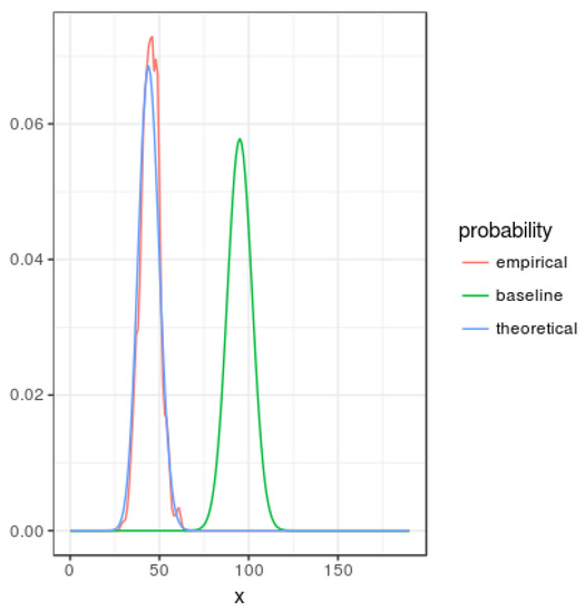
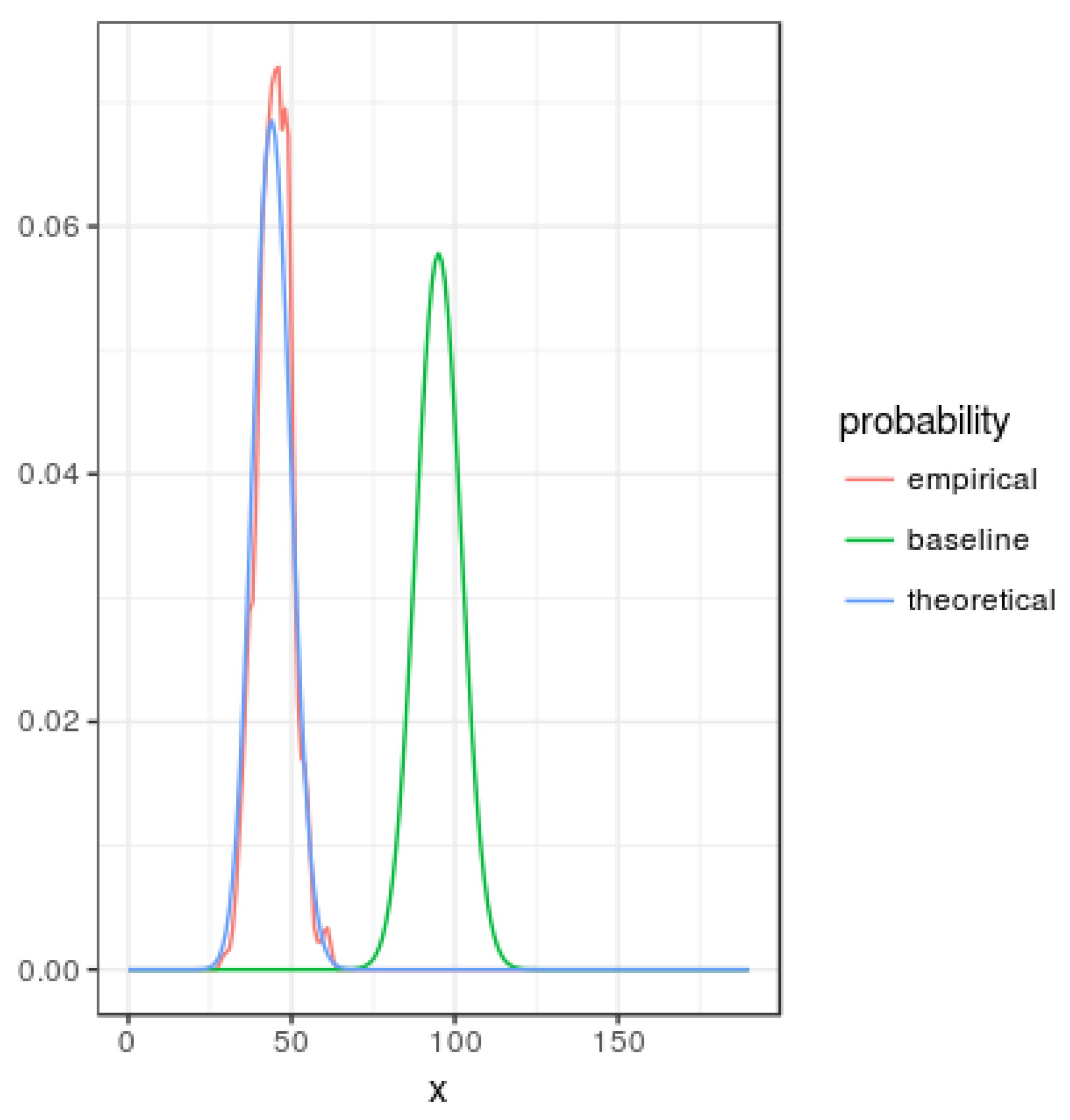
Figure 1 represents smoothed probability mass functions for the baseline, theoretical given by Equation (23) and empirical (based in simulations) with and . Note that asymmetry of the u value generates a probability function with less entropy than the corresponding to the baseline mass function.
Figure 1.
Comparison among smoothed probability mass functions: baseline, theoretical and empirical for and .
Repeating a similar procedure to Equations (19) and (20) the corresponding entropy can be computed as
which for becomes .
4.3.1. Alternative Simple Model
Another simple model could assume that whenever an existing edge is selected to be removed, it is removed with probability , whereas, alternatively, a new edge is randomly added. The transition matrix of the corresponding for the number of links would be
Note that an equivalent symmetric model can be defined as follows. If the selected a pair of nodes does not have an associated link, we add such a link with probability , otherwise an existing link is removed.
It can be proved that the resulting stationary distribution has the form:
which can be seen as another generalization of the binomial distribution via the new parameter . Again the network cross-sectional entropy can be computed as
Both models Equations (22) and (24) provide respectively stationary distributions Equations (23) and (25) which, in general, are not binomial. Therefore, if we take a snapshot of these stationary distributions, the resulting network will follow a new static model, different from the standard known reference models for static networks.
Note that again these models can be interpreted as urn-derived finite state discrete-time birth-death models, in the sense that they do not incorporate network structural information, but only the total number of links. In other words, these models do not differentiate among networks that belong to the same equivalence class .
5. Simulations for the Time Evolution of Features
Numerical simulations have been performed to characterize the time evolution of the number of links, the clustering coefficient and the entropy of the sample degree distribution for the extended model defined by Equation (22).
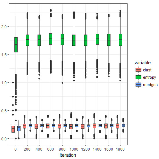
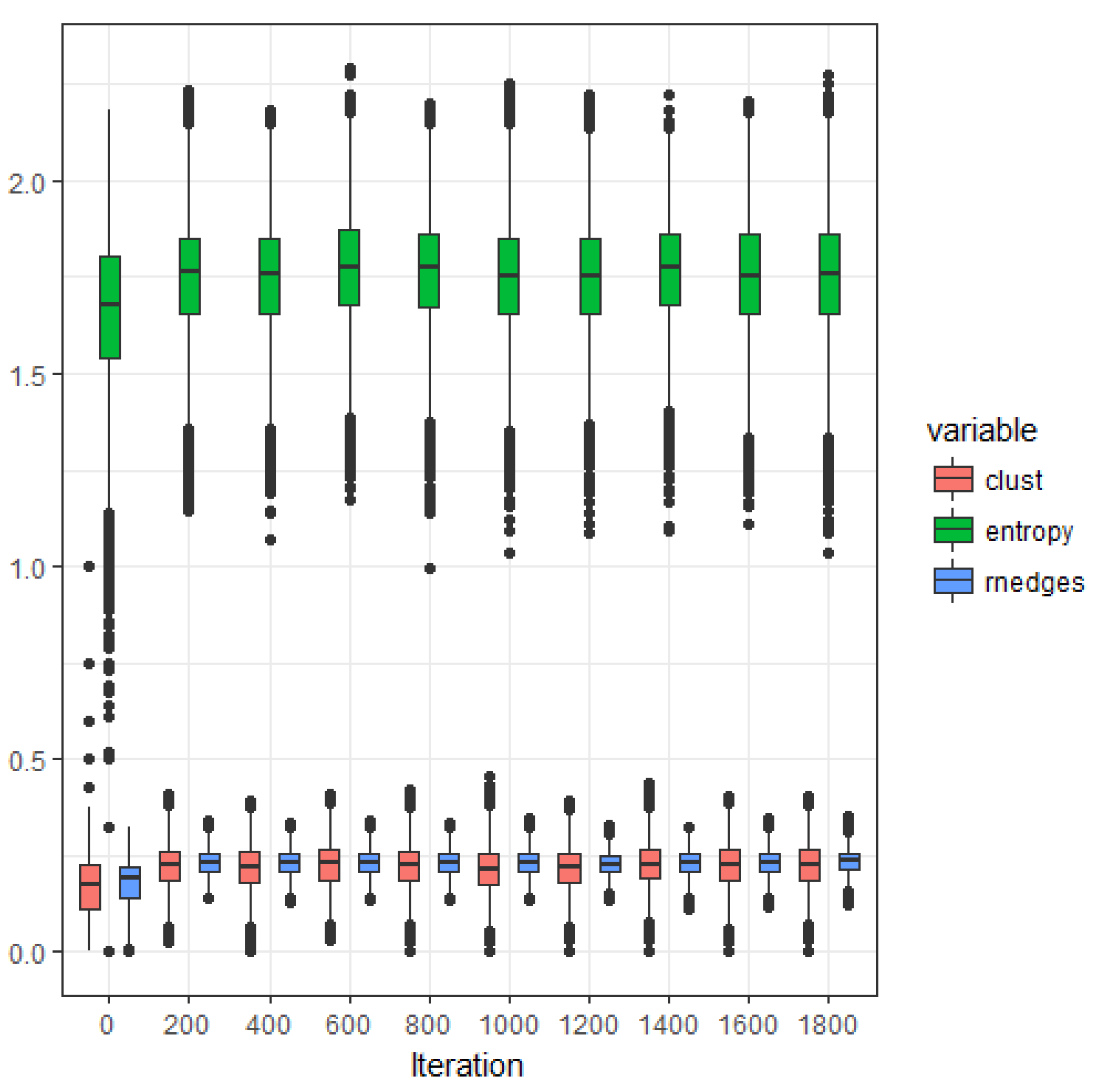
Figure 2 shows the evolution (starting from the empty graph) of the relative number of edges (number of edges divided by the maximum possible number of edges), the clustering coefficient and the samples degree distribution entropy of a graph that evolves following the extended model defined by Equation (22) with and . The estimations of relative number of edges and clustering coefficient converge to the same stationary value as the iteration number increases; note that the variance of the clustering coefficient is significantly larger than the variance corresponding the relative number of edges. The estimated degree distribution presents also a significant variance.
Figure 2.
Estimated expected values of relative number of edges, clustering coefficient and sample degree distribution entropy, as a function of the iteration number ( and ).
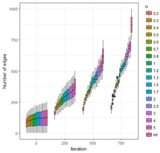
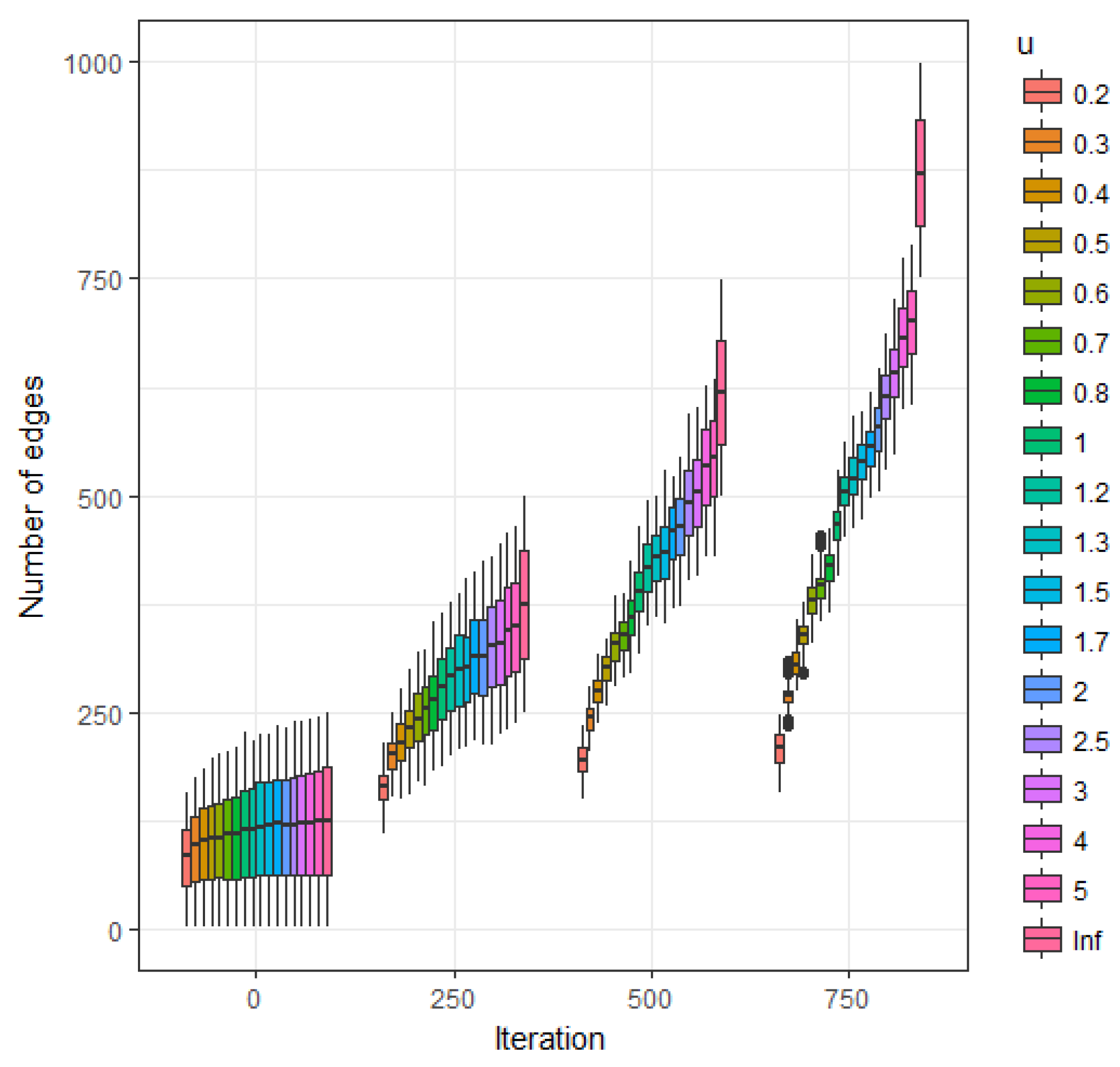
Figure 3 represents the estimated expected value of the number of edges as a function of iteration number (starting from the empty graph) and parameter u. Due to the uniform nature of the behavior of the clustering coefficient follows a similar behavior.
Figure 3.
Estimated expected value of number of edges as a function of u at iterations 250, 500, 750 and 1000.
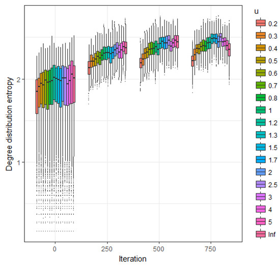
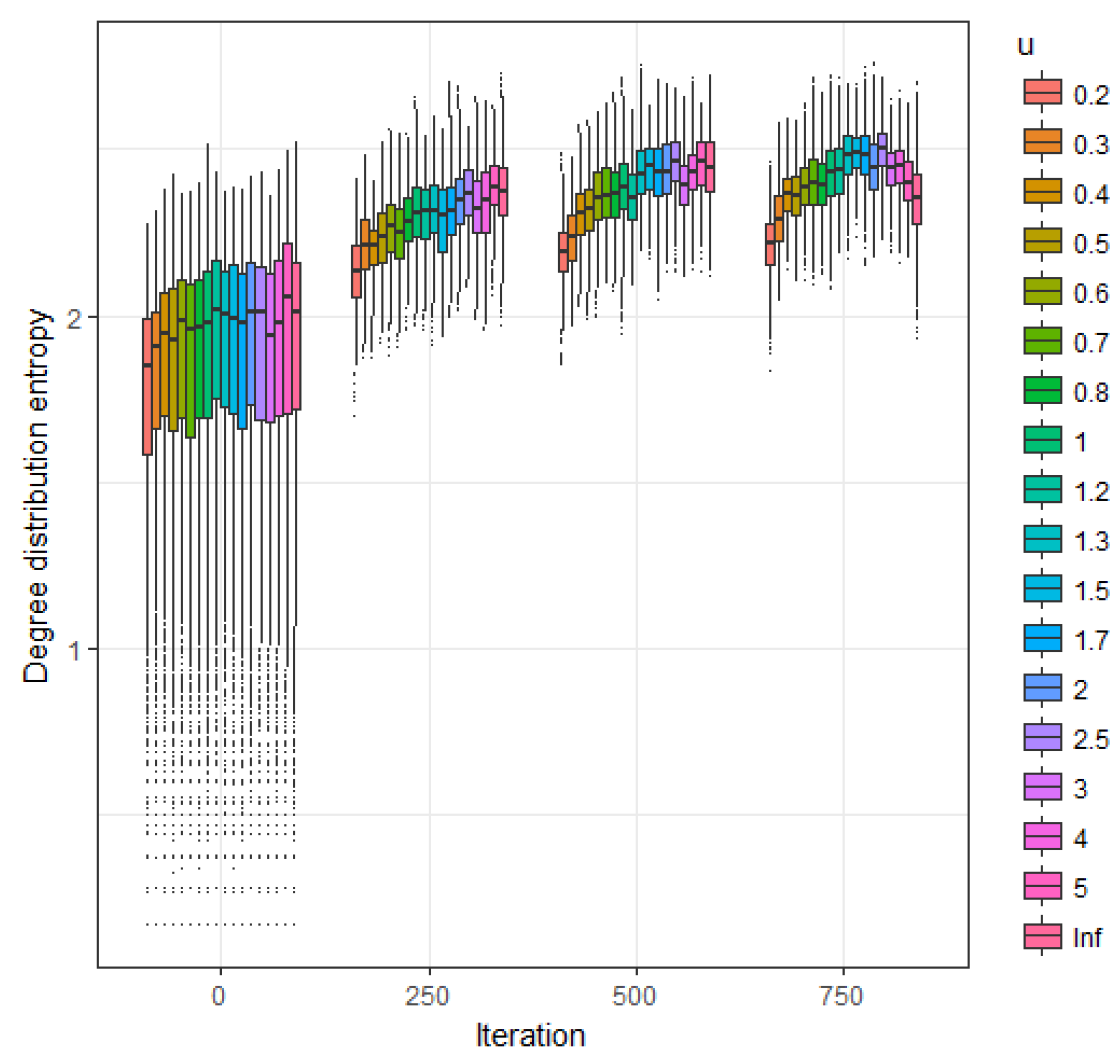
Figure 4 represents the estimated expected value of the sample degree distribution entropy as a function of iteration number (starting from the empty graph) and parameter u. Larger values are obtained for as also illustrated in Figure 1.
Figure 4.
Estimated expected value of the sample degree distribution entropy as function of u at iterations 250, 500, 750 and 1000.
6. Concluding Remarks
Several basic models for dynamic networks have been proposed and analyzed in terms of the cross-sectional entropy, and time evolution of the number of links, clustering coefficient and entropy of the sample degree distribution. The evolution of these features seems to be useful to characterize the proposed models. Such models can serve as a reference baseline for future research on more complex models for time evolving networks.
Author Contributions
Pedro J. Zufiria developed the theoretical content, wrote the document and helped with the simulations. Iker Barriales-Valbuena developed the simulations and helped with the theoretical content and the writing of the paper.
Acknowledgments
This work has been partially supported by project MTM2015-67396-P of Ministerio de Economía y Competitividad, Spain.
References
- Siljak, D.D. Dynamic Graphs. Nonlinear Anal. Hybrid Syst. 2008, 2, 544–567. [Google Scholar] [CrossRef] [Scilit]
- Holme, P.; Saramäki, J. Temporal networks. Phys. Rep. 2012, 519, 97–125. [Google Scholar] [CrossRef] [Scilit]
- Rahmani, A.; Ji, M.; Mesbahi, M.; Egerstedt, M. Controllability of multi-agent systems from a graph-theoretic perspective. SIAM J. Control Optim. 2009, 48, 162–186. [Google Scholar] [CrossRef] [Scilit]
- Zufiria, P.J.; Barriales-Valbuena, I. Evolution models for dynamic networks. In Proceedings of the 2015 38th International Conference on Telecommunications and Signal Processing (TSP), Prague, Czech, 9–11 July 2015; pp. 252–256. [Google Scholar]
- Zufiria, P.J.; Barriales-Valbuena, I. Entropy Characterization of Random Network Models. Entropy 2017, 19, 321. [Google Scholar] [CrossRef] [Scilit]
- Klein, M.J. Entropy and the Ehrenfest urn model. Physica 1956, 22, 569–575. [Google Scholar]
- van Doorn, E.A.; Schrijner, P. Geometric ergodicity and quasi-stationarity in discrete-time birth-death processes. ANZIAM J. 1995, 37, 121–144. [Google Scholar]
- Feller, W. An Introduction to Probability Theory and Its Applications; Wiley: Hoboken, NJ, USA, 1968; Volume 1. [Google Scholar]
- Johnson, N.L.; Kemp, A.W.; Kotz, S. Univariate Discrete Distributions; John Wiley & Sons: Hoboken, NJ, USA, 2005; Volume 444. [Google Scholar]
- Kemp, A.W. Steady-state Markov chain models for certain q-confluent hypergeometric distributions. J. Stat. Plan. Inference 2005, 135, 107–120. [Google Scholar] [CrossRef] [Scilit]
- Morimoto, T. Markov processes and the H-theorem. J. Phys. Soc. Jpn. 1963, 18, 328–331. [Google Scholar] [CrossRef] [Scilit]
Publisher’s Note: MDPI stays neutral with regard to jurisdictional claims in published maps and institutional affiliations. |
© 2018 by the authors. Licensee MDPI, Basel, Switzerland. This article is an open access article distributed under the terms and conditions of the Creative Commons Attribution (CC BY) license (https://creativecommons.org/licenses/by/4.0/).