A New Look at the Capacitor Theory

Abstract

The mathematical description of the charging process of time-varying capacitors is reviewed and a new formulation is proposed. For it, suitable fractional derivatives are described. The case of fractional capacitors that follow the Curie–von Schweidler law is considered. Through suitable substitutions, a similar scheme for fractional inductors is obtained. Formulae for voltage/current input/output are presented. Backward coherence with classic results is established and generalised to the variable order case. The concept of a tempered fractor is introduced and related to the Davidson–Cole model.

1. Introduction

Resistors, capacitors and inductors are the fundamental building blocks of basic electric circuits. The laws that underlie their physical behaviour are assumed to be well known. This does not mean that they cannot be called into question when some new result or theory is introduced. This is the recent case concerning the problem of charge storage in capacitors, mainly the fractional ones that follow the Curie–von Schweidler law [1,2]. Two new recently proposed modelling formulae have been subject of some discussion [3,4,5,6,7]. Of course, the two perspectives are clearly different and irreconcilable. A careful reading of both approaches leads us to identify some origins of the different visions and search for an alternative. Firstly, the fractional derivative used in such approaches is not suitable for solving the problem. In fact, the Caputo derivative has several drawbacks [8,9], but the main ones are the confusion between the Heaviside unit step and the constant function, leading to results contradicted by experience [10] and the Caputo derivative of a sinusoid is not a sinusoid [8,11]. Another problem we encounter is the forgetfulness of the past that leads to some mistakes in the use of distribution theory. Here, we tackle the problem and propose a coherent alternative that generalises the classical results.

Traditionally, a formula, deduced from the Maxwell equations, relates the charge, $q\left(t\right),t\in \mathbb{R}$, and voltage, $v\left(t\right),$ in a capacitor. It reads

$$q\left(t\right)=Cv\left(t\right),$$

(1)

where C is the capacitance expressed in Farad (F). This formula, obtained under stationary conditions, expresses a static relation between two physical entities. In reality, the underlying dynamics is not visible. However, it appears in the relationship between $q\left(t\right)$ and the current, $i\left(t\right)$, as we will see later. In practice, the above relation expresses an approximation that is good enough in many situations. We will assume that it characterises order 1 ideal capacitors. The discussed problem, introduced first by S. Das [3,12], consists of a generalisation of the previous relation to the case where the capacitance varies with time, $C=c\left(t\right),t\in \mathbb{R}$. It would be expected that we should write

$$q\left(t\right)=c\left(t\right)v\left(t\right),$$

(2)

but S. Das denied it and proposed

$$q\left(t\right)=c\left(t\right)\ast v\left(t\right)={\int }_{-\infty }^{t}c\left(\tau \right)v(t-\tau )\mathrm{d}\tau ,$$

(3)

as an alternative [3,4,13]. Recently [5,7], V. Pandey proposed another way of dealing with the problem that reads

$$q\left(t\right)=c\left(t\right)\ast v^{\prime }\left(t\right)={\int }_{-\infty }^{t}c\left(\tau \right)v^{\prime }(t-\tau )\mathrm{d}\tau ,$$

(4)

where $v^{\prime }\left(t\right)=\frac{dv\left(t\right)}{dt}$ is the usual derivative. This has given rise to a discussion that promises to be interesting and that we intend to continue here. In fact, we believe that these two new proposals are not the best solution to the problem. It is interesting to note, attending to the properties of the convolution, that (4) can be rewritten as

$$\frac{d^{-1}q\left(t\right)}{d{t}^{-1}}=c\left(t\right)\ast v\left(t\right),$$

highlighting the incompatibility of the three approaches, (2)–(4).

To find an alternative, we will consider (2) as the correct solution, as long as we assume (1) to properly characterise an ideal integer order time-invariant capacitor. For the ideal time-variant fractional capacitor, none of the above solutions are appropriate.

We will face the problem with generality. Firstly, we show the correctness of (2) for order 1 capacitor and, from the dimensional analysis of the involved entities, we introduce a coherent solution. Our approach will be based on the use of fractional derivatives of Liouville type [11,14], discarding the most known Riemann–Liouville and Caputo derivatives. We revise the problem and discuss two different situations corresponding to which magnitude is considered as input/output: current or voltage. This involves the capacitance or its inverse. The obtained formulation is transported to the magnetic field giving rise to an analogous inductor theory. Going on with generalisations, we propose a framework for variable order capacitors and coils.

A brief analysis of the stability of the fractor leads us to propose the use of the tempered fractor [15]. This new operator is related with the Davidson–Cole model.

The paper outlines as follows. In Section 2, we present a brief introduction to the fractors and to the fractional derivatives suitable to our objective: the study of the capacitors that we perform in Section 3, considering the order 1 and fractional. Profiting the obtained results, we introduce an analog formulation for the coil modelling (Section 4). The formulae for the input/output relations are introduced in Section 5. We extend the formulation for variable order fractors through suitable derivatives in Section 7. In Section 8, the concept of tempered fractor is proposed. Finally, in Section 9 we present some conclusions.

Remarks

We assume that

• Our working domain is always $\mathbb{R}$.
• We use the bilateral Laplace transform (LT):

  $$\mathcal{L}\left[f\left(t\right)\right]=F\left(s\right)=\underset{-\infty }{\overset{\infty }{\int }}f\left(t\right)e^{-st}\mathrm{d}t,$$

  (5)

  where $f\left(t\right)$ is any real or complex function defined on $\mathbb{R}$ and $F\left(s\right)$ is its transform, provided it has a non-void region of convergence (ROC).
• The Fourier transform is obtained from the LT through the substitution $s=j\omega$ with $\omega \in \mathbb{R}$ and $j=\sqrt{-1}$.
• The inverse LT is given by the Bromwich integral

  $$f\left(t\right)={\mathcal{L}}^{-1}\left[F\left(s\right)\right]=\frac{1}{2\pi j}\underset{a-j\infty }{\overset{a+j\infty }{\int }}F\left(s\right)e^{st}\mathrm{d}s,t\in \mathbb{R},$$

  (6)

  where $a\in \mathbb{R}$ is inside the region of convergence of the LT.
• Current properties of the Dirac delta distribution, $\delta \left(t\right)$, and its derivatives will be used.
• The order of the fractional derivative is assumed to be any real number.
• The multi-valued expression $s^{\alpha }$ is used. To obtain a function we will fix for a branch-cut line the negative real half axis and select the first Riemann surface.
• It is very common to add the prefix pseudo” to the “fractionalisation” of classic entities, as is also the case for "capacitance", which appears as “pseudo-capacitance”. We do not find any particular reason to do so [1].

2. Fractional Devices and Derivatives

2.1. The Differintegrator

The elemental system, with transfer function (TF) $G\left(s\right)=s^{\alpha },\alpha \in \mathbb{R},$ is called differintegrator [11], fractor [16,17,18,19], or constant phase element (CPE) [20,21,22,23,24,25]. It is very important in modelling real systems [18,22,26,27,28,29,30,31]. If $Re\left(s\right)>0,$ it will be called forward, otherwise, if $Re\left(s\right)<0,$ it will be denoted backward. In the following, we will consider the forward case only, since it is causal.

The impedance of a circuit element involving only a differintegrator is called fractance and assumes the form

$$Z\left(j\omega \right)=K_{\alpha }{\left(j\omega \right)}^{\alpha }.$$

For non-integer order, $\alpha ,$ it is a complex function. An ideal fractional inductor ($\alpha >0$) has fractance [18,30,31]

$$Z_L=L_{\alpha }{\left(j\omega \right)}^{\alpha }$$

where $L_{\alpha }$ is the inductance, expressed in $\left[H·s^{1-\alpha }\right]$. Similarly, an ideal fractional capacitor has fractance [1,2]

$$Z_C=\frac{1}{C_{\alpha }{\left(j\omega \right)}^{\alpha }},$$

where the capacitance $C_{\alpha }$ has units $\left[F/s^{1-\alpha }\right].$ With $\alpha =1$, we obtain the classic inductor and capacitor reactances.

For any real order, the inverse LT of the $G\left(s\right)$ is given by [11,32]

$${\mathcal{L}}^{-1}{s}^{\alpha }=\frac{t^{-\alpha -1}}{\Gamma (-\alpha )}\epsilon \left(t\right),$$

(7)

where $\epsilon \left(t\right)$ denotes the Heaviside unit step. It is important to highlight the positive order cases which lead to singular distributions. In particular, a given positive integer order, n, gives [33]:

$${\delta }^{\left(n\right)}\left(t\right)=\frac{t^{-n-1}}{(-n-1)!}\epsilon \left(t\right),n\ge 0.$$

(8)

Remark 1.

It is important to note that the parallel or series association of fractors is a fractor only if they have the same order. If we combine two or more different order fractors, we obtain systems that are described by more complex models. This is the case of the supercapacitors [20,21,34] or the electrochemical capacitors [20,27,29].

2.2. Suitable Fractional Derivatives

The differintegrator is an operator, $D^{\alpha }={\displaystyle \frac{d^{\alpha }}{d{t}^{\alpha }}},$ such that

$$\mathcal{L}\left[D^{\alpha }f\left(t\right)\right]=s^{\alpha }F\left(s\right),Re\left(s\right)\ge 0,$$

(9)

where $F\left(s\right)=\mathcal{L}\left[f\left(t\right)\right].$ For a positive order, we will call it a fractional derivative (FD). The negative order operator will be called anti-derivative. If $Re\left(s\right)\ge 0$ [32],

$$s^{\alpha }=\underset{h\to 0^{+}}{lim}{h}^{-\alpha }{\left(1-e^{-sh}\right)}^{\alpha },$$

where

$${\left(1-e^{-sh}\right)}^{\alpha }=\sum _{n=0}^{+\infty }\frac{{\left(-\alpha \right)}_n}{n!}{e}^{-nsh}.$$

The symbol ${\left(-\alpha \right)}_n$ is the Pochhamer representation of the raising factorial: ${\left(-\alpha \right)}_0=1,$${\left(-\alpha \right)}_n={\prod }_{k=0}^{n-1}\left(-\alpha +k\right).$ Using the inverse LT, we obtain

$$D^{\alpha }f\left(t\right)=\underset{h\to 0^{+}}{lim}{h}^{-\alpha }\sum _{n=0}^{+\infty }\frac{{\left(-\alpha \right)}_n}{n!}f(t-nh),$$

(10)

that is called Grünwald–Letnikov (GL) derivative, in spite of their first proposal having been done by Liouville [35]. Relation (9) suggests another way of expressing the FD using the impulse response of the causal differintegrator. Thus, we define FD as the output of the differintegrator to a given function, $f\left(t\right),$ through the convolution

$$D^{\alpha }f\left(t\right)=\frac{1}{\Gamma (-\alpha )}\underset{0}{\overset{\infty }{\int }}{\tau }^{-\alpha -1}f(t-\tau )d\tau .$$

(11)

For negative orders, the relation (11) defines the anti-derivative. However, when $\alpha >0$ (derivative case) the integral kernel, ${\tau }^{-\alpha -1},$ has a singularity at the origin, requiring regularising actions. The regularised Liouville derivative is given by [11]

$$D^{\alpha }f\left(t\right)=\underset{0}{\overset{\infty }{\int }}\frac{{\tau }^{-\alpha -1}}{\Gamma (-\alpha )}\left[f(t-\tau )-\sum _{m=0}^N\frac{{(-1)}^m{f}^{\left(m\right)}\left(t\right)}{m!}{\tau }^m\right]d\tau ,$$

(12)

where $N\in {\mathbb{Z}}_0^{+}$ is the greatest integer less than or equal to $\alpha$, so that $N\le \alpha <N+1$. If $N<0$, the summation is null. For $\alpha =n\in {\mathbb{Z}}^{+},$ we are led to use the relation (8), but we obtain an almost useless expression. However, we have two alternatives for applying the convolution, avoiding the singularity. Let $\alpha \le M\in {\mathbb{Z}}_0^{+}$. We can write

$$s^{\alpha }=s^{\alpha -M}{s}^M=s^M{s}^{\alpha -M},$$

which gives us two ways to solve the problem. The first reads [36]

$$D^{\alpha }f\left(t\right)=\underset{0}{\overset{\infty }{\int }}\frac{{\tau }^{M-\alpha -1}}{\Gamma (-\alpha +M)}{f}^{\left(M\right)}(t-\tau )d\tau .$$

(13)

This is called Liouville–Caputo derivative [36,37]. The second decomposition, $s^{\alpha }=s^M{s}^{\alpha -M}$, gives

$$D^{\alpha }f\left(t\right)=D^M\left[\underset{0}{\overset{\infty }{\int }}\frac{{\tau }^{M-\alpha -1}}{\Gamma (-\alpha +M)}f(t-\tau )d\tau \right],$$

(14)

that constitutes a derivative of the Riemann–Liouville type, that is also called Liouville derivative [38], or Liouville–Weyl [39]. Therefore, from the impulse response of the differintegrator, three different integral formulations were obtained from where current expressions can be derived, (12), (13), and (14). We will opt for the first [14] and particularise it for the $0<\alpha <1$ case.

$$D^{\alpha }f\left(t\right)=\underset{0}{\overset{\infty }{\int }}\frac{{\tau }^{-\alpha -1}}{\Gamma (-\alpha )}\left[f(t-\tau )-f\left(t\right)\right]d\tau .$$

(15)

Example 1.

Consider the sinusoidal function $f\left(t\right)=e^{j\omega t}$. Then

$$D^{\alpha }{e}^{j\omega t}=\underset{0}{\overset{\infty }{\int }}\frac{{\tau }^{-\alpha -1}}{\Gamma (-\alpha )}\left[e^{j\omega (t-\tau )}-e^{j\omega t}\right]d\tau =e^{j\omega t}\frac{1}{\Gamma (-\alpha )}\underset{0}{\overset{\infty }{\int }}\left[e^{-j\omega \tau }-1\right]{\tau }^{-\alpha -1}d\tau .$$

(16)

It can be shown that the integral equals ${\left(j\omega \right)}^{\alpha }\Gamma (-\alpha )$ [32].

3. On the Capacitor

3.1. Classic: $q\left(t\right)=c\left(t\right)v\left(t\right)$

The capacitor is a device used to store electrical charge. Traditionally, the main equation describing the capacitor behaviour is (2) that we rewrite here

$$q\left(t\right)=C_{0}v\left(t\right),$$

where $q\left(t\right),C_0,v\left(t\right),(t\in \mathbb{R}),$ are the charge, capacitance, and voltage, respectively, and with SI unities, Coulomb (C), Farad (F), and Volt (V). The electric current is defined as the time derivative of the charge:

$$i\left(t\right)={\displaystyle \frac{dq\left(t\right)}{dt}}.$$

(17)

The unit of electric current is the ampere (A ≡ Cs${}^{-1}$). Therefore,

$$q\left(t\right)={\int }_{-\infty }^{t}i\left(u\right)\mathrm{d}u,$$

(18)

leading to

$$v\left(t\right)={\displaystyle \frac{1}{C_0}}{\int }_{-\infty }^{t}i\left(u\right)\mathrm{d}u.$$

(19)

Consider a capacitor with two metallic plates separated by air. As known, the capacitance of these capacitors is proportional to the inverse of the distance between the plates. Assume we insert such a capacitor, having a charge $q_0,$ in an open circuit. Suppose now, that the plates are linearly spaced (d) so that the capacity decreases inversely. As the charge is constant, the voltage increases in the same way:

$$q_0=C_0{v}_0={\displaystyle \frac{C_0}{1+d}}{v}_0(1+d)$$

If $d=at,a>0,t\ge 0$, $v\left(t\right)=v_0(1+at)$.

Now, imagine that we perform the same operation, but close the circuit with a constant voltage generator. In this situation, the voltage remains constant, but the charge decreases similarly $q\left(t\right)={\displaystyle \frac{q_0}{1+at}}$.

Let us assume that the capacitance is, for $t\ge 0$, a piecewise constant function

$$c\left(t\right)=\left\{\begin{array}{cc}{C}_0\hfill & 0\le t<t_0\hfill \\ C_1\hfill & t_0\le t<t_1\hfill \\ \cdots \hfill & \cdots \hfill \\ C_n\hfill & t_{n-1}\le t<t_n\hfill \\ \cdots \hfill & \cdots \hfill \end{array}\right.=\sum _{n=0}^{\infty }{C}_n{p}_n\left(t\right),$$

(20)

where $p_n\left(t\right)=\epsilon (t-t_{n-1})-\epsilon (t-t_n).$ Let $v\left(t\right)$ be the applied voltage. Therefore, for a given interval $(t_{n-1}-t_n)$, the charge $q_{(}t)$ is equal to $C_n{p}_n\left(t\right)v\left(t\right)$. Joining the contributions from all the intervals, we have:

$$q\left(t\right)=\sum _{n=0}^{\infty }\left[C_n{p}_n\left(t\right)v\left(t\right)\right]=\sum _{n=0}^{\infty }\left[C_n{p}_n\left(t\right)\right]v\left(t\right)$$

Therefore, the correct way of expressing relation between charge and voltage is

$$q\left(t\right)=c\left(t\right)v\left(t\right),$$

(21)

provided that capacitor is not fractional. In this situation, the current is given by

$$i\left(t\right)={\displaystyle \frac{d\left[c\left(t\right)v\left(t\right)\right]}{dt}}$$

(22)

and the voltage is

$$v\left(t\right)={\displaystyle \frac{1}{c\left(t\right)}}{\int }_{-\infty }^{t}i\left(u\right)\mathrm{d}u.$$

(23)

3.2. Fractional: $\frac{d^{1-\alpha }q\left(t\right)}{d{t}^{1-\alpha }}=c\left(t\right)v\left(t\right)$

For orders $0<\alpha <1$, the (fractional) capacitors are based on the Curie–von Schweidler law describing by a power law the decay of a depolarising current in a dielectric that is subjected to a step DC voltage, $v\left(t\right)=V_0\epsilon \left(t\right)$, [1,2,16,20,21]:

$$i\left(t\right)=K_0{V}_0{t}^{-\alpha }\epsilon \left(t\right),$$

(24)

where $K_0$ is a constant related to the capacitance. The fractional derivative of the Heaviside unit step is given by [32]

$${\displaystyle \frac{d^{\alpha }\epsilon \left(t\right)}{d{t}^{\alpha }}}={\displaystyle \frac{t^{-\alpha }}{\Gamma (1-\alpha )}}\epsilon \left(t\right).$$

Therefore, in the time invariant case, we can write

$$i\left(t\right)=C_0{\displaystyle \frac{d^{\alpha }v\left(t\right)}{d{t}^{\alpha }}}.$$

(25)

$C_0$ is the (fractional) capacitance. Using the LT, we obtain

$$I\left(s\right)=C_0{s}^{\alpha }V\left(s\right).$$

(26)

Consequently, the impedance is

$$Z\left(s\right)={\displaystyle \frac{1}{C_0{s}^{\alpha }}},$$

(27)

as expected. Attending to (26), we obtain

$$Q\left(s\right)={\displaystyle \frac{I\left(s\right)}{s}}=C_0{s}^{\alpha -1}V\left(s\right)$$

and

$$s^{1-\alpha }Q\left(s\right)=C_{0}V\left(s\right),$$

which leads to

$${\displaystyle \frac{d^{1-\alpha }q\left(t\right)}{d{t}^{1-\alpha }}}=C_{0}v\left(t\right),$$

(28)

Now, consider the piecewise constant capacitance (20) and note that (28) represents a linear equation, so the superposition principle is valid. For t in the interval, $(t_{n-1},t_n)$ the charge, $q_n\left(t\right)$, is expressed by:

$${\displaystyle \frac{d^{1-\alpha }{q}_n\left(t\right)}{d{t}^{1-\alpha }}}=C_n{p}_n\left(t\right)v\left(t\right),$$

that gives

$$q_n\left(t\right)={\int }_{-\infty }^t{C}_n{p}_n\left(\tau \right)v\left(\tau \right){\displaystyle \frac{{(t-\tau )}^{-\alpha }}{\Gamma (1-\alpha )}}d\tau .$$

Defining $q\left(t\right)$ by

$$q\left(t\right)=\sum _{n=0}^{\infty }{q}_n\left(t\right),$$

we have

$$q\left(t\right)=\sum _{n=0}^{\infty }{\int }_{-\infty }^t{C}_n{p}_n\left(\tau \right)v\left(\tau \right){\displaystyle \frac{{(t-\tau )}^{-\alpha }}{\Gamma (1-\alpha )}}d\tau .$$

Permuting the summation and integral operations, valid because the integral is finite, we obtain

$$q\left(t\right)={\int }_{-\infty }^t\sum _{n=0}^{\infty }{C}_n{p}_n\left(\tau \right)v\left(\tau \right){\displaystyle \frac{{(t-\tau )}^{-\alpha }}{\Gamma (1-\alpha )}}d\tau ,$$

and

$$q\left(t\right)={\int }_{-\infty }^{t}c\left(\tau \right)v\left(\tau \right){\displaystyle \frac{{(t-\tau )}^{-\alpha }}{\Gamma (1-\alpha )}}d\tau .$$

This relation together with (21) suggest we write

$${\displaystyle \frac{d^{1-\alpha }q\left(t\right)}{d{t}^{1-\alpha }}}=c\left(t\right)v\left(t\right),$$

(29)

as a general charge–voltage relation. It is important to note that the existence of the fractional derivative serves to highlight the causality and memory of the system [2,40].

To verify the coherence of (29), note that the capacitance is expressed in $[F/s^{1-\alpha }],$ which implies that the right-hand side has a dimension $[F/s^{1-\alpha }]V=FV/s^{1-\alpha }=C/s^{1-\alpha }$ in agreement with the left-hand side. Relation (29) contradicts the approaches introduced in [3,4,5,7]. As we observe, formulae (25)–(29) degenerate in the corresponding classic, as discussed in Section 3.1, when $\alpha =1$. Therefore, we will continue with them.

3.3. A Strange Result

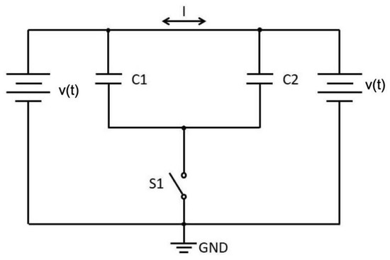
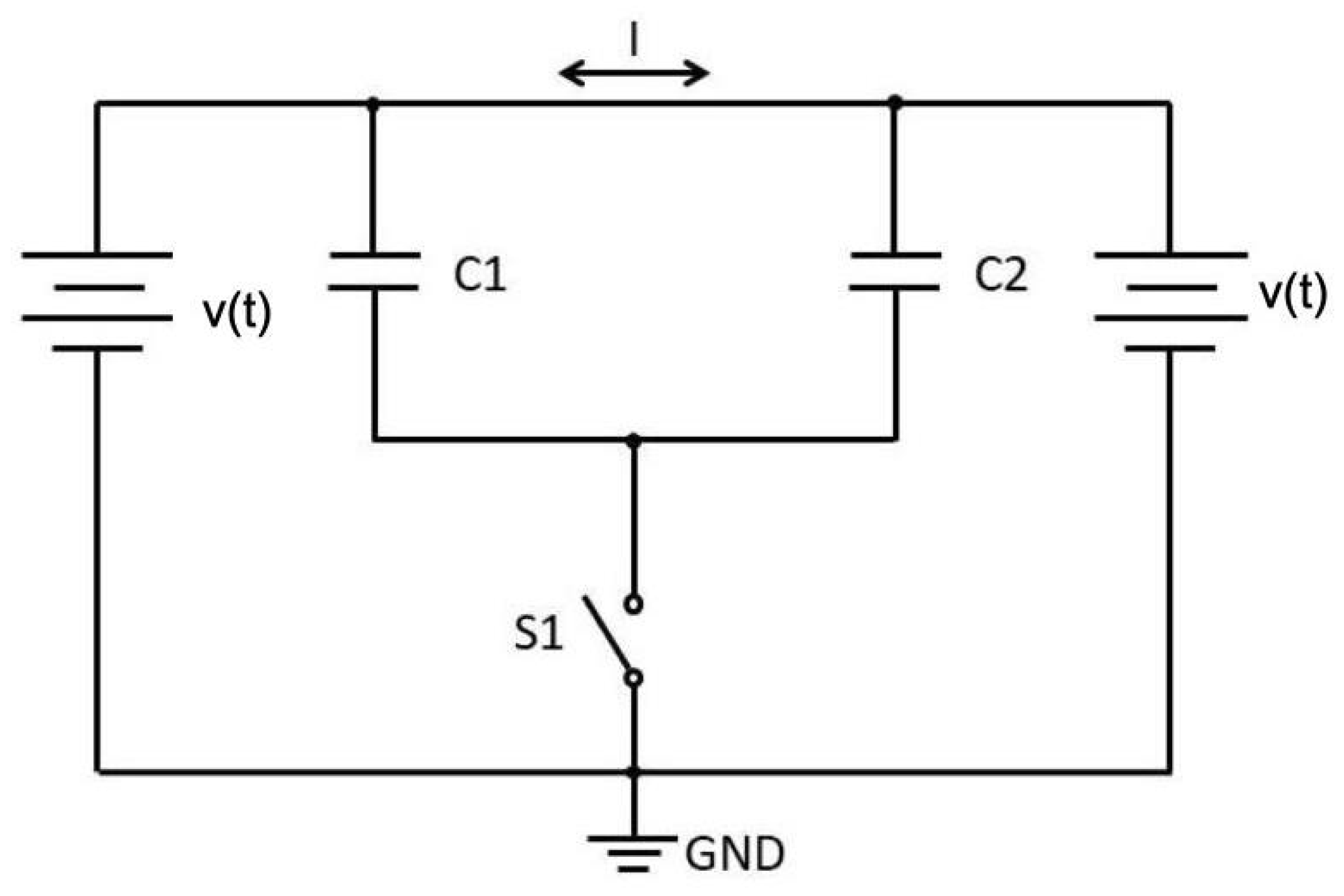
Let two capacitors, with different constant capacitances and orders, be associated in parallel and submitted to the voltage $v\left(t\right)$—see Figure 1.

Figure 1. Two capacitor (pseudo-)symmetric circuit. Is $I\equiv 0$?

From (28), we have:

$${\displaystyle \frac{d^{1-{\alpha }_1}{q}_1\left(t\right)}{d{t}^{1-{\alpha }_1}}}{\displaystyle \frac{1}{C_1}}={\displaystyle \frac{d^{1-{\alpha }_2}{q}_2\left(t\right)}{d{t}^{1-{\alpha }_2}}}{\displaystyle \frac{1}{C_2}}$$

and

$${\displaystyle \frac{d^{-{\alpha }_1}{i}_1\left(t\right)}{d{t}^{-{\alpha }_1}}}{\displaystyle \frac{1}{C_1}}={\displaystyle \frac{d^{-{\alpha }_2}{i}_2\left(t\right)}{d{t}^{-{\alpha }_2}}}{\displaystyle \frac{1}{C_2}}$$

Assume that ${\alpha }_1<{\alpha }_2$, so that we can write

$${\displaystyle \frac{d^{{\alpha }_2-{\alpha }_1}{q}_1\left(t\right)}{d{t}^{{\alpha }_2-{\alpha }_1}}}={\displaystyle \frac{C_1}{C_2}}{q}_2\left(t\right)$$

and

$${\displaystyle \frac{d^{{\alpha }_2-{\alpha }_1}{i}_1\left(t\right)}{d{t}^{{\alpha }_2-{\alpha }_1}}}={\displaystyle \frac{C_1}{C_2}}{i}_2\left(t\right)$$

The expected charges and currents are $q_1\left(t\right)={\displaystyle \frac{C_1}{C_2}}{q}_2\left(t\right)$ and $i_1\left(t\right)={\displaystyle \frac{C_1}{C_2}}{i}_2\left(t\right),$ but with ${\alpha }_1\ne {\alpha }_2$, we must have an unexpected current since

$${\displaystyle \frac{d^{{\alpha }_2-{\alpha }_1}{i}_1\left(t\right)}{d{t}^{{\alpha }_2-{\alpha }_1}}}-i_1\left(t\right)\ne 0,$$

We performed several laboratory experiments without successful results. It is expected that such a difference is small, because $|{\alpha }_2-{\alpha }_1|$ is also small.

4. On the Fractional Inductor

The relations (17) and (29) that completely define the fractional capacitor can be used to introduce the fractional inductor [30,31,41] through suitable substitutions. Let $\psi \left(t\right)$ be the magnetic flux (in $W_b$) and $l\left(t\right)$ the inductance (expressed in $H.s^{1-\alpha }.$) Perform the following substitutions in the relations (25) to (29)

$$\psi \left(t\right)\to q\left(t\right),$$

$$l\left(t\right)\to c\left(t\right),$$

$$i\left(t\right)\to v\left(t\right).$$

From (17), we obtain

$$v\left(t\right)={\displaystyle \frac{d\psi \left(t\right)}{dt}},$$

(30)

while (29) gives

$${\displaystyle \frac{d^{1-\alpha }\psi \left(t\right)}{d{t}^{1-\alpha }}}=l\left(t\right)i\left(t\right).$$

(31)

In the time-invariant case, $l\left(t\right)=L_0,$ we obtain

$${\displaystyle \frac{d^{1-\alpha }\psi \left(t\right)}{d{t}^{1-\alpha }}}=L_{0}i\left(t\right),$$

(32)

that degenerates into the classic relation

$$\psi \left(t\right)=L_{0}i\left(t\right),$$

(33)

when $\alpha =1$, giving

$$v\left(t\right)=L_0{\displaystyle \frac{di\left(t\right)}{dt}}.$$

(34)

Remark 2.

In the previous two sections, we assumed that the order verifies $0<\alpha \le 1$. However, there is no theoretical reason to assume such a constraint. All the above relations keep their validity if $\alpha >1$, provided we use the derivatives introduced in Section 2.2 [14,19].

5. Responses of Fractional Ideal Capacitor

5.1. Formulation

The relations (25)–(29), introduced above, define what we will call an ideal (fractional) capacitor. In the following, we will work in this framework. We have two ways of rewriting (29) according to which function is considered as input:

1.

Voltage

$$i\left(t\right)={\displaystyle \frac{d^{\alpha }\left[c\left(t\right)v\left(t\right)\right]}{d{t}^{\alpha }}},$$

(35)

where $i\left(t\right)$ is the output.

2.

Current

$$v\left(t\right)={\displaystyle \frac{1}{c\left(t\right)}}{\displaystyle \frac{d^{-\alpha }}{d{t}^{-\alpha }}}i\left(t\right),$$

(36)

where $v\left(t\right)$ is the output.

The Leibniz rule allows us to express the above fractional derivatives in terms of integer order derivatives and fractional anti-derivatives of the involved factors [11]. We will use a simplified approach in agreement with the physics of the process. Firstly, consider the traditional situation where $c\left(t\right)=C_0$, a real constant. In this case, the capacitor becomes a differintegrator with transfer function (impedance), from (36)

$$H\left(s\right)={\displaystyle \frac{V\left(s\right)}{I\left(s\right)}}={\displaystyle \frac{1}{C_0{s}^{\alpha }}},Re\left(s\right)>0,$$

(37)

where $V\left(s\right)$ and $I\left(s\right)$ are the Laplace transforms of the voltage and current intensity. The corresponding impulse response is:

$$h_c\left(t\right)={\displaystyle \frac{t^{\alpha -1}}{C_0\Gamma \left(\alpha \right)}}\epsilon \left(t\right).$$

(38)

Obviously, the impulse response corresponding to (35) is obtained with the change $-\alpha$ for $\alpha$. In such a case, the impulse response is not absolutely integrable. So, the corresponding system is unstable. This means that we must be careful in using Equation (35).

Remark 3.

Similarly, considering (30), we are led to the equations corresponding to the responses of the fractional inductor

$$v\left(t\right)={\displaystyle \frac{d^{\alpha }\left[l\left(t\right)i\left(t\right)\right]}{d{t}^{\alpha }}}$$

(39)

and

$$i\left(t\right)={\displaystyle \frac{1}{l\left(t\right)}}{\displaystyle \frac{d^{-\alpha }v\left(t\right)}{d{t}^{-\alpha }}}.$$

(40)

5.2. The Voltage Input Case

Let us consider a capacitor with variable capacitance. Note that the device must have been assembled some time ago. Therefore, its capacitance will always change in its proper time $\theta$:

$$c\left(\theta \right)=C_0+c_v\left(\theta \right).$$

(41)

where $C_0>0$. $C_v\left(\theta \right)>-C_0$ is a function that expresses the long-term capacitance variation. We assume that $C_v\left(\theta \right)$ is slowly variable in time (lowpass function). Let $v\left(t\right),t\in \mathbb{R}$. We define the output current intensity through the convolution:

$$i\left(t\right)=\frac{1}{\Gamma (-\alpha )}{\int }_0^{\infty }{\tau }^{-\alpha -1}c(t-\tau )\left[v(t-\tau )-v\left(t\right)\right]d\tau ,t\in \mathbb{R}.$$

(42)

Remark 4.

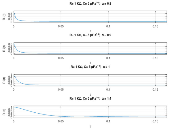
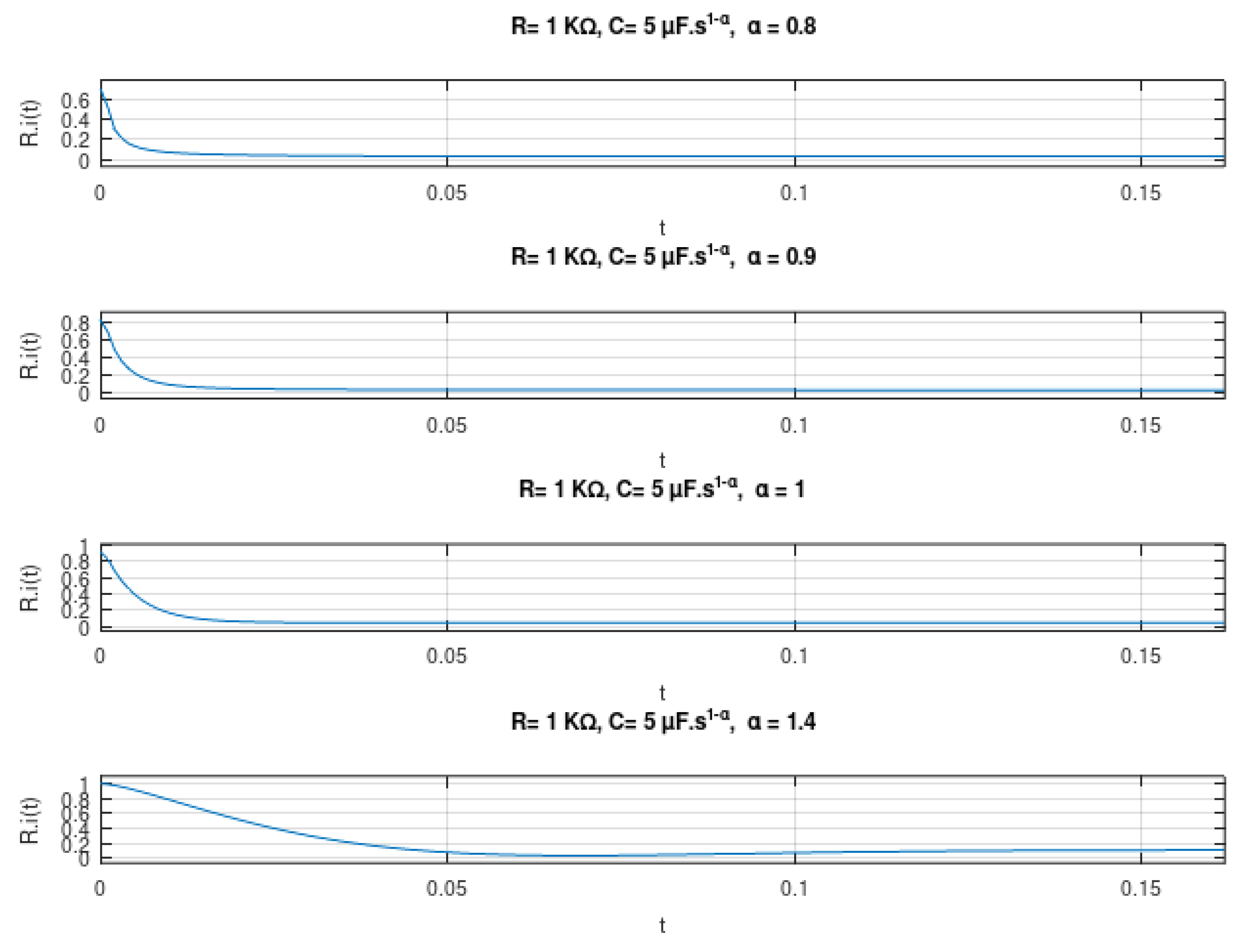
The framework we described is theoretical. In practice, it is very difficult to connect a capacitor to an ideal voltage step, because, at the time of the transition, it would be necessary for the source to supply an infinite current (24). In a practical circuit, there is always some non-zero series resistance, as the internal resistance of the source and the parasitic series resistance of the capacitor, which will significantly affect (reduce) the resulting current in the time of transition, even if this resistance is very small. This also affects the charge time course, and the mathematical relations presented become imprecise. The RC circuit can serve to model the effect of such resistances. This is illustrated in Figure 2 where the currents in an RC circuit are depicted.

Figure 2. Normalised current, $R.i\left(t\right)$, in an RC circuit.

Example 2.

To examplify, assume that the capacitance is constant, $c\left(t\right)=C_0,$ and $v\left(t\right)=V_0\epsilon \left(t\right)$. Then

$$\begin{array}{cc}\hfill i\left(t\right)=& \frac{C_0}{\Gamma (-\alpha )}{\int }_0^{\infty }{\tau }^{-\alpha -1}\left[\epsilon (t-\tau )-\epsilon \left(\tau \right)\right]d\tau \hfill \\ \hfill =& -\frac{C_0}{\Gamma (-\alpha )}{\int }_t^{\infty }{\tau }^{-\alpha -1}d\tau =\frac{C_0}{\Gamma (-\alpha +1)}{\tau }^{-\alpha }\epsilon \left(\tau \right).\hfill \end{array}$$

that expresses the Curie–von Schweidler law [2,5].

Example 3.

Consider piecewise constant case:

$$c\left(t\right)=\left\{\begin{array}{cc}{A}_1\hfill & t<t_0\hfill \\ A_2\hfill & t\ge t_0\hfill \end{array}\right.=A_1\epsilon \left(t\right)+\left[A_2-A_1\right]\epsilon (t-t_0)$$

(43)

We obtain

$$\begin{array}{cc}\hfill i_v\left(t\right)& =\frac{A_1}{\Gamma (-\alpha )}{\int }_0^{t_0}{\tau }^{-\alpha -1}\left[v(t-\tau )-v\left(t\right)\right]d\tau +\frac{A_2}{\Gamma (-\alpha )}{\int }_{t_0}^{\infty }{\tau }^{-\alpha -1}\left[v(t-\tau )-v\left(t\right)\right]d\tau \hfill \\ \hfill & =\frac{A_1}{\Gamma (-\alpha )}{\int }_0^{\infty }{\tau }^{-\alpha -1}\left[v(t-\tau )-v\left(t\right)\right]d\tau +\frac{A_2-A_1}{\Gamma (-\alpha )}{\int }_{t_0}^{\infty }{\tau }^{-\alpha -1}\left[v(t-\tau )-v\left(t\right)\right]d\tau \hfill \\ \hfill & =A_1{D}^{\alpha }v\left(t\right)+\frac{A_2-A_1}{\Gamma (-\alpha )}{\int }_{t_0}^{\infty }{\tau }^{-\alpha -1}\left[v(t-\tau )-v\left(t\right)\right]d\tau \epsilon (t-t_0).\hfill \end{array}$$

(44)

This expression can be generalised for any set of jumps.

Example 4.

Being a lowpass function, we can assume that $c_v\left(t\right)$ is a sum of exponentials:

$$c_v\left(\theta \right)=\sum _{k=1}^N{A}_k{e}^{-{\lambda }_k\theta }\epsilon (\theta -{\theta }_{0k}),$$

(45)

where $A_k,{\lambda }_k,k=1,2,\cdots ,N$ are positive constants and ${\theta }_{0k}$ reference instants. For simplicity, we will study the $N=1$ case.

Therefore, we can rewrite the second term (41) as

$$\begin{array}{cc}\hfill i_v\left(t\right)& =\frac{A}{\Gamma (-\alpha )}{\int }_0^{\infty }{\tau }^{-\alpha -1}{e}^{-\lambda \tau }\left[u(t-\tau )-u\left(\tau \right)\right]d\tau \hfill \\ \hfill & =\frac{A}{\Gamma (-\alpha )}{\int }_t^{\infty }{\tau }^{-\alpha -1}{e}^{-\lambda \tau }d\tau =\frac{A{t}^{-\alpha }{e}^{-\lambda t}}{\Gamma (-\alpha +1)}\epsilon \left(t\right),\hfill \end{array}$$

(46)

that is the regularised tempered fractional derivative of $v\left(t\right)$, $D_{\lambda }^{\alpha }v\left(t\right)$ [15].

Remark 5.

It is not very difficult to show that a substitution of each exponential by a sinusoid leads to a similar solution, provided we extend the definition of a tempered derivative accordingly.

$$D_{j\lambda }^{\alpha }f\left(t\right)=\frac{1}{\Gamma (-\alpha )}{\int }_0^{\infty }{\tau }^{-\alpha -1}{e}^{-j\lambda \tau }f(t-\tau )d\tau .$$

(47)

These results can be generalised for any capacitance with Laplace or Fourier transforms. In fact, returning to (41), we have

$$i\left(t\right)=\frac{C_0}{\Gamma (-\alpha )}{\int }_0^{\infty }{\tau }^{-\alpha -1}\left[v(t-\tau )-v\left(\tau \right)\right]d\tau +\frac{1}{\Gamma (-\alpha )}{\int }_0^{\infty }{\tau }^{-\alpha -1}{c}_v(t-\tau )\left[v(t-\tau )-v\left(\tau \right)\right]d\tau .$$

(48)

The first term, which we can call static component, is basically the $\alpha -$order derivative of $v\left(t\right)$:

$$i_0\left(t\right)=C_0\frac{d^{\alpha }v\left(t\right)}{d{t}^{\alpha }}=\frac{C_0}{\Gamma (-\alpha )}{\int }_0^{\infty }{\tau }^{-\alpha -1}\left[v(t-\tau )-v\left(\tau \right)\right]d\tau .$$

(49)

To treat the other, assume that the variable part of the capacitance $c_v\left(t\right)$ has LT, $C_v\left(s\right),Re\left(s\right)>a,a\le 0$. The Bromwich integral allows us to write:

$$c_v\left(t\right)=\frac{1}{2\pi j}{\int }_{\sigma -j\infty }^{\sigma +j\infty }{C}_v\left(s\right)e^{st}\mathrm{d}s,t\in \mathbb{R},$$

(50)

where the principal value of the integral is assumed and $\sigma >0$. We can write

$${\int }_0^{\infty }{\tau }^{-\alpha -1}{c}_v(t-\tau )\left[v(t-\tau )-v\left(\tau \right)\right]d\tau =\frac{1}{2\pi j}{\int }_{\sigma -j\infty }^{\sigma +j\infty }{C}_v\left(s\right){\int }_0^{\infty }{\tau }^{-\alpha -1}{e}^{s(t-\tau )}\left[v(t-\tau )-v\left(\tau \right)\right]d\tau \mathrm{d}s.$$

The inner integral is the tempered derivative of $v\left(t\right)$ [15], so that

$$i_v\left(t\right)=\frac{1}{2\pi j}{\int }_{\sigma -j\infty }^{\sigma +j\infty }{C}_v\left(s\right)e^{st}{D}_s^{\alpha }v\left(t\right)\mathrm{d}s,t\in \mathbb{R},$$

(51)

with

$$D_s^{\alpha }v\left(t\right)={\int }_0^{\infty }{\tau }^{-\alpha -1}{e}^{-s\tau }\left[v(t-\tau )-v\left(\tau \right)\right]d\tau ,t\in \mathbb{R}.$$

(52)

These expressions are so general that they lack usefulness. We are going to consider particular cases for $c_v\left(t\right)$.

Example 5.

An interesting particular case comes in consideration of a linearly increasing capacitance:

$$c_v\left(t\right)=C_{v0}t\epsilon \left(t\right)$$

We obtain:

$$\begin{array}{cc}\hfill i_v\left(t\right)& =\frac{C_{v0}}{\Gamma (-\alpha )}{\int }_0^{\infty }{\tau }^{-\alpha -1}(t-\tau )\epsilon (t-\tau )\left[v(t-\tau )-v\left(\tau \right)\right]d\tau \hfill \\ & =\frac{C_{v0}}{\Gamma (-\alpha )}{\int }_0^t{\tau }^{-\alpha -1}(t-\tau )\left[v(t-\tau )-v\left(\tau \right)\right]d\tau \hfill \\ & =C_{v0}t\epsilon \left(t\right)D^{\alpha }\left[v\left(t\right)\epsilon \left(t\right)\right]-\alpha C_{v0}{D}^{\alpha -1}\left[v\left(t\right)\epsilon \left(t\right)\right]\hfill \end{array}$$

If $v\left(t\right)={\displaystyle \frac{t^{\alpha }}{\Gamma (\alpha +1)}}\epsilon \left(t\right)$, then

$$D^{\alpha }v\left(t\right)=\epsilon \left(t\right),D^{\alpha -1}v\left(t\right)=t\epsilon \left(t\right)$$

and

$$i_v\left(t\right)=(1-\alpha )C_{v0}t\epsilon \left(t\right),$$

is a curious result that agrees with the considerations we made in Section 3.1. The $v\left(t\right)=\epsilon \left(t\right)$ case is readily obtained from the results presented in Section 2.2.

5.3. The Current Input Case

In the above sub-section, we developed a formalism based on relation (35), where we considered the voltage as input and the current as output. Now, we reverse the situation by starting from (36). The main differences are

1.

The use of the fractional anti-derivative ($\alpha <0$) that is defined by a regular integral:

$$\begin{array}{cc}\hfill v\left(t\right)=& \frac{1}{\Gamma \left(\alpha \right)c\left(t\right)}{\int }_0^{\infty }{\tau }^{\alpha -1}i(t-\tau )d\tau \hfill \\ \hfill =& \frac{1}{\Gamma \left(\alpha \right)c\left(t\right)}{\int }_{-\infty }^{t}i\left(\tau \right){(t-\tau )}^{\alpha -1}d\tau ;\hfill \end{array}t\in \mathbb{R}.$$

(53)

2.

The involvement of the function $\frac{1}{c\left(t\right)}$ does not add complexity to the situation.

Example 6.

Considering the constant capacitance case $c\left(t\right)=C_0$, we obtain

$$v\left(t\right)=\frac{1}{\Gamma \left(\alpha \right)C_0}{\int }_{-\infty }^{t}i\left(\tau \right){(t-\tau )}^{\alpha -1}d\tau$$

(54)

which generalises, for any $\alpha ,$ the classic result

$$v\left(t\right)=\frac{1}{C_0}{\int }_{-\infty }^{t}i\left(\tau \right)d\tau .$$

Example 7.

Return to the situation defined in (43)

$${\displaystyle \frac{1}{c\left(t\right)}}=\left\{\begin{array}{cc}\frac{1}{A_1}\hfill & t<t_0\hfill \\ \frac{1}{A_2}\hfill & t\ge t_0\hfill \end{array}\right.=\frac{1}{A_1}\epsilon \left(t\right)+\left[\frac{1}{A_2}-\frac{1}{A_1}\right]\epsilon (t-t_0).$$

We obtain

$$\begin{array}{cc}\hfill v\left(t\right)& =\frac{1}{\Gamma \left(\alpha \right)A_1}{\int }_{-\infty }^{t_0}i\left(\tau \right){(t-\tau )}^{\alpha -1}d\tau +\frac{1}{\Gamma \left(\alpha \right)A_2}{\int }_{t_0}^{t}i\left(\tau \right){(t-\tau )}^{\alpha -1}d\tau \hfill \\ \hfill & =\frac{1}{\Gamma \left(\alpha \right)A_1}{\int }_{-\infty }^{t}i\left(\tau \right){(t-\tau )}^{\alpha -1}d\tau +\frac{1}{\Gamma \left(\alpha \right)(\frac{1}{A_2}-\frac{1}{A_1})}{\int }_{t_0}^{t}i\left(\tau \right){(t-\tau )}^{\alpha -1}d\tau .\hfill \end{array}$$

(55)

The first term corresponds to the constant capacitance case, while the second expresses the effect in the capacitance jump.

6. Power and Energy

We proceed to study the power and energy flux in a capacitor [42]. For simplicity, we will consider the time-invariant case. As usual, we define the (instantaneous) power by

$$p\left(t\right)=v\left(t\right)i^{\ast }\left(t\right),$$

(56)

where we have considered the possibility of complex signals. In the following, we will deal with real signals unless clearly stated. Assume that $v\left(t\right)$ and $i\left(t\right)$ are signals with finite energy (energy-type signal) [43], having a Fourier transform, $V\left(i\omega \right)$ and $I\left(i\omega \right)$, respectively. The energy is given by

$$\mathcal{E}={\int }_{-\infty }^{\infty }v\left(t\right)i\left(t\right)\mathrm{d}t.$$

(57)

The Parseval relation allows us to write

$$\mathcal{E}={\displaystyle \frac{1}{2\pi }}{\int }_{-\infty }^{\infty }V\left(j\omega \right)I(-j\omega )\mathrm{d}\omega .$$

(58)

The relation between the voltage and current allows us to obtain

$$\mathcal{E}={\displaystyle \frac{C_0}{2\pi }}{\int }_{-\infty }^{\infty }{(-j\omega )}^{\alpha }{\left|V\left(j\omega \right)\right|}^2\mathrm{d}\omega ,$$

(59)

since $V(-j\omega )=V{\left(j\omega \right)}^{\ast }$. However,

$${(-j\omega )}^{\alpha }={\left|\omega \right|}^{\alpha }{e}^{-j\alpha \frac{\pi }{2}\mathit{sgn}\left(\omega \right)},$$

where $\mathit{sgn}\left(\omega \right)=2u\left(\omega \right)-1$ is the signum function, so that

$$\mathcal{E}={\displaystyle \frac{C_{0}cos\left(\alpha \frac{\pi }{2}\right)}{2\pi }}{\int }_{-\infty }^{\infty }{\left|\omega \right|}^{\alpha }{\left|V\left(j\omega \right)\right|}^2\mathrm{d}\omega$$

(60)

This result seems to be strange, since, if $\alpha =1$, the energy is null, but gives a positive energy in the other cases. To understand the reason, we must remember that $v\left(t\right)$ has finite energy. This means that it is a pulse-like signal that decreases to zero. Therefore, we conclude that the order 1 ideal capacitor charges and decharges, without there being any loss of energy. On the contrary, in the fractional case, there is always some energy lost that increases with decreasing $\alpha$.

We continue the energetic study, by considering the case of “power-type” signals. Let $v\left(t\right)=\epsilon \left(t\right)$. In this case, the power is

$$p\left(t\right)=i\left(t\right)=C_0{D}^{\alpha }\epsilon \left(t\right)=C_0\frac{t^{-\alpha }}{\Gamma (-\alpha +1)}\epsilon \left(t\right),$$

and the energy is

$$\mathcal{E}=C_0{\int }_0^{\infty }\frac{t^{-\alpha }}{\Gamma (-\alpha +1)}dt.$$

(61)

We have two different situations

1.

$\alpha =1$

The integrand degenerates into a $\delta \left(t\right)$ and the integral gives 1. Thus, the energy is $\mathcal{E}=C_0$.

2.

$\alpha <1$

$$\mathcal{E}=C_0{\left.\frac{t^{1-\alpha }}{\Gamma (2-\alpha )}\right|}_0^{\infty }=\infty ,$$

(62)

as expected.

We go on with the study of the steady-state behaviour of the ideal fractional capacitor using power-type signals. We consider a sinusoid first and then an almost periodic signal [43]. Let $v\left(t\right)=A{e}^{j{\omega }_{0}t},{\omega }_0>0,t\in \mathbb{R}.$ Then

$$p\left(t\right)=A^2{C}_0{e}^{j{\omega }_{0}t}{(-j{\omega }_0)}^{\alpha }{e}^{-j{\omega }_{0}t}={(-j{\omega }_0)}^{\alpha }{A}^2{C}_0.$$

If $v\left(t\right)=Acos\left({\omega }_{0}t\right)$, then

$$p\left(t\right)=2|{\omega }_0{|}^{\alpha }cos\left(\alpha \frac{\pi }{2}\right)A^2{C}_0,$$

showing that the power is constant. Therefore, the energy is infinite, apart from the $\alpha =1$ case. This result may not be interesting. We modify the reasoning. Note that the mean power supplied to the capacitor is

$$\mathcal{P}=\underset{T\to \infty }{lim}{\displaystyle \frac{1}{2T}}{\int }_{-T}^{T}p\left(t\right)dt=\underset{T\to \infty }{lim}{\displaystyle \frac{1}{2T}}{\int }_{-T}^{T}2|{\omega }_0{|}^{\alpha }cos\left(\alpha \frac{\pi }{2}\right)A^2{C}_{0}dt=2{\left|{\omega }_0\right|}^{\alpha }cos\left(\alpha \frac{\pi }{2}\right)A^2{C}_0.$$

This result shows that the mean power is also constant. It is important to remark the strangeness of the integer order case, where both energy and power are null. This happens because, without losses, the energy spent in one half-period is recovered in the next.

Let $v\left(t\right)$ be an almost periodic signal:

$$v\left(t\right)=\sum _{m=-\infty }^{\infty }{V}_m{e}^{j{\omega }_{m}t},$$

where we assume that

• $t\in \mathbb{R}$;
• ${\omega }_m=-{\omega }_{-m},m\in \mathbb{Z}$;
• $V_{-m}=V_m^{\ast },m\in \mathbb{Z}$;
• ${\sum }_{m=-\infty }^{\infty }{\left|V_m\right|}^2<\infty .$

Under these conditions and using the results in [43], we conclude that the mean power is

$$\mathcal{P}=C_{0}cos\left(\alpha \frac{\pi }{2}\right)\sum _{m=-\infty }^{\infty }|{\omega }_m{|}^{\alpha }{\left|V_m\right|}^2,$$

that can be considered as a generalisation of the Parseval relation.

7. Variable Order Capacitors and Inductors

The variable order capacitors were studied, for the first time, in [17], using a Riemann–Liouville derivative. Here, we consider the above framework. All the above equations describing the behaviour of both capacitors and inductors remain valid in the variant order case, provided suitable definitions are used. In fact, it is a simple task to verify this statement using the variable order GL or Liouville derivatives [11,44]. The variable order GL derivative is given by:

$$D^{\alpha \left(t\right)}f\left(t\right)=\underset{h\to 0^{+}}{lim}{h}^{-\alpha \left(t\right)}\sum _{k=0}^{\infty }\frac{{(-\alpha \left(t\right))}_k}{k!}f(t-kh).$$

(63)

This definition preserves a very important property of the fractional derivatives previously introduced. Let $f\left(t\right)=e^{st},s\in \mathbb{C}$,

$$D^{\alpha \left(t\right)}{e}^{st}=\underset{h\to 0^{+}}{lim}{h}^{-\alpha \left(t\right)}\sum _{k=0}^{\infty }\frac{{(-\alpha \left(t\right))}_k}{k!}{e}^{s(t-kh)}=s^{\alpha \left(t\right)}{e}^{st},\mathrm{for}Re\left(s\right)>0.$$

(64)

The variable order regularised Liouville derivative reads [11,44]

$$D^{\alpha }f\left(t\right)=\frac{1}{\Gamma (-\alpha (t\left)\right)}\underset{0}{\overset{\infty }{\int }}{\tau }^{-\alpha \left(t\right)-1}\left[f(t-\tau )-\epsilon \left(\alpha \left(t\right)\right)\sum _0^{N\left(t\right)}\frac{{(-1)}^m{f}^{\left(m\right)}\left(t\right)}{m!}{\tau }^m\right]d\tau ,$$

(65)

where $N\left(t\right)\le \alpha \left(t\right)N\left(t\right)+1.$ This expression includes both the positive and negative values of $\alpha \left(t\right)$. In the negative case, the summation is null. Therefore, we can interpret (65) as a variable order differintegral. In particular, if $0<\alpha \left(t\right)<1,$ then we obtain

$$D^{\alpha }f\left(t\right)=\frac{1}{\Gamma (-\alpha (t\left)\right)}\underset{0}{\overset{\infty }{\int }}{\tau }^{-\alpha \left(t\right)-1}\left[f(t-\tau )-f\left(t\right)\right]d\tau .$$

(66)

With these derivatives, we can obtain variable order impedances, for both capacitors and inductors:

$$Z_c\left(s\right)={\displaystyle \frac{1}{C_0{s}^{\alpha \left(t\right)}}},Z_i\left(s\right)=L_0{s}^{\alpha \left(t\right)}.$$

(67)

The responses of these devices can be obtained from the above introduced theory and using the results in [44].

8. Tempered Fractors

Return back to (25) and note that the charge corresponding a unit step input is given by:

$$q\left(t\right)=C_0{\displaystyle \frac{t^{1-\alpha }\epsilon \left(t\right)}{\Gamma (2-\alpha )}}.$$

(68)

As seen, it is an increasing function, which points out that the fractional capacitor is not a stable system. A permanent increase in the charge is not to be expected [1]. This is a consequence of the fact that the fractor is an ideal system. Such a situation does not occur with real capacitors where we have to introduce a non-zero conductance in parallel with the fractor. This can be achieved through what we call tempered fractor, which is defined by

$$Z_T\left(s\right)=C_0{(s+\lambda )}^{\alpha },$$

(69)

where $\lambda$ is a (small) positive number of dimension $\left[s^{-1}\right]$.

The LT inverse of $Z_T\left(s\right)$ is given by [15]

$$z_T\left(t\right)=K_{\alpha }{e}^{-\lambda t}\frac{t^{-\alpha -1}}{\Gamma (-\alpha )}\epsilon \left(t\right).$$

(70)

This function decreases to zero, for any value of $\alpha$. With it, we define the tempered fractional derivatives that we can use to substitute the derivatives used in the previous sections. For example, (53) reads

$$v\left(t\right)=\frac{1}{\Gamma \left(\alpha \right)c\left(t\right)}{\int }_0^{\infty }{e}^{-\lambda \tau }{\tau }^{\alpha -1}i(t-\tau )d\tau .$$

(71)

It is interesting to remark that the well-known Davidson–Cole model represents a tempered fractor [18,45,46]. In fact, the model can be written as [46]

$$Z_{DC}\left(j\omega \right)={\displaystyle \frac{1}{{\left(1+j\omega \tau \right)}^{\alpha }}},$$

where $\tau$ is a time constant. We can write

$$Z_{DC}\left(j\omega \right)={\displaystyle \frac{1/{\tau }^{\alpha }}{{\left(\frac{1}{\tau }+j\omega \right)}^{\alpha }}},$$

highlighting the presence of the tempered fractor.

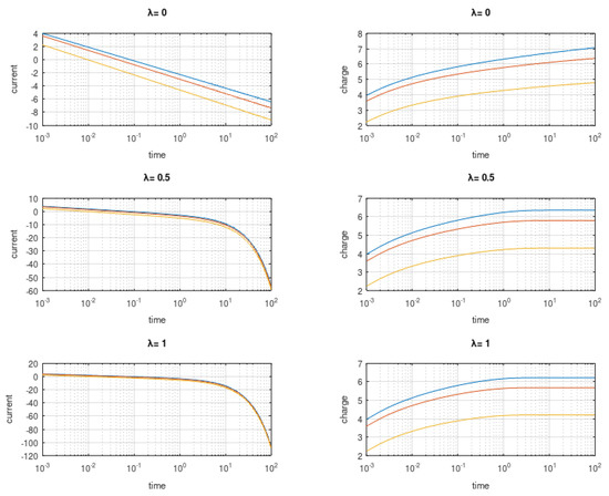
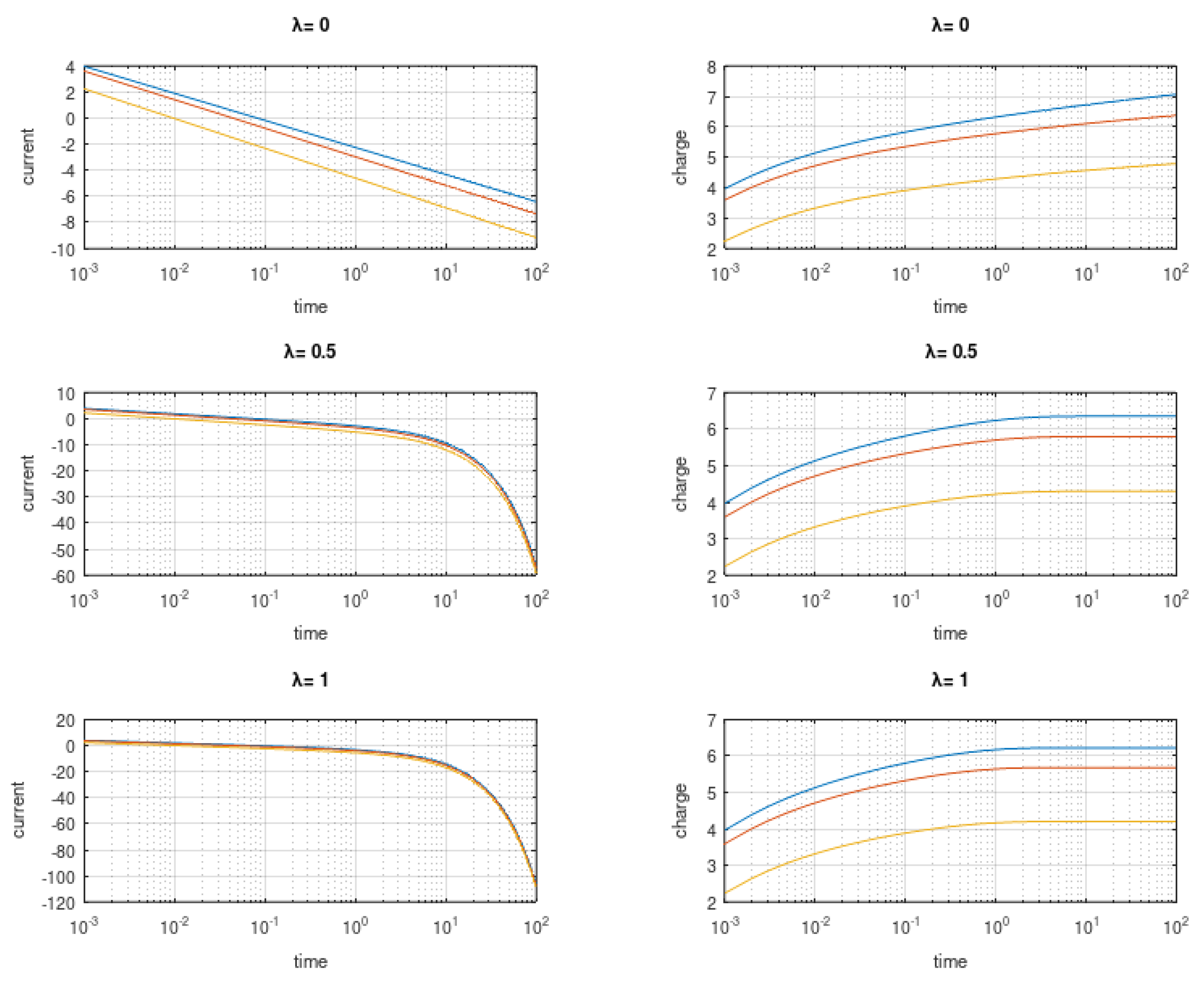
In Figure 3, we illustrate the similarities and differences between the ideal fractor and its tempered analog by computing the current and charge in both situations, using the expression obtained in Example 2 and its tempered version:

$$i\left(t\right)=\frac{C_0}{\Gamma (-\alpha +1)}{e}^{-\lambda t}{t}^{-\alpha }\epsilon \left(t\right).$$

Figure 3. The behaviour of the tempered fractor for $\alpha =[0.9,0.95,0.99]$, from top to bottom.

For simplicity (and far from practical reality), we made $C_0=1F/s^{1-\alpha }.$ As seen, the exponential does not introduce a meaningful modification in the current, but forces the charge to approach a constant. For easy visualisation, we represented the logarithm of the current and charge on a logarithmic scale.

9. Conclusions

The Liouville fractional calculus was used to review the mathematical description of the charging process in capacitors. A new formulation was proposed to establish the memory effect. For it, suitable, among many, fractional derivatives were described. The case of fractional capacitors that follow the Curie–von Schweidler law was considered and studied. Through suitable substitutions a similar scheme for fractional inductors was obtained. Formulae for voltage/current input/output were presented. Backward coherence with classic results was established and generalised to the variable order case. The concept of tempered fractor was introduced and related to the Davidson–Cole model.

References

- Westerlund, S.; Ekstam, L. Capacitor Theory. IEEE Trans. Dielectr. Electr. Insul. 1994, 1, 826–839. [Google Scholar] [CrossRef] [Scilit]
- Westerlund, S. Dead Matter Has Memory; Causal Consulting: Kalmar, Sweden, 2002. [Google Scholar]
- Das, S. A new look at formulation of charge storage in capacitors and application to classical capacitor and fractional capacitor theory. Asian J. Res. Rev. Phys. 2018, 1, 1–18. [Google Scholar] [CrossRef] [Scilit]
- Das, S. Theoretical verification of formula for charge function in time q=c*v in RC circuit for charging/discharging of fractional & ideal capacitor. Theory Appl. Phys. Sci. 2019, 1, 1–44. [Google Scholar]
- Pandey, V. Origin of the Curie–von Schweidler law and the fractional capacitor from time-varying capacitance. J. Power Sources 2022, 532, 231309. [Google Scholar] [CrossRef] [Scilit]
- Allagui, A.; Elwakil, A.S.; Psychalinos, C. Comment on “Origin of the Curie–von Schweidler law and the fractional capacitor from time-varying capacitance” [J. Pow. Sources 532 (2022) 231309]. J. Power Sources 2022, 551, 232166. [Google Scholar] [CrossRef] [Scilit]
- Pandey, V. Response to “Comment on ‘Origin of the Curie–von Schweidler law and the fractional capacitor from time-varying capacitance [J. Power Sources 532 (2022) 231309]’”. J. Power Sources 2022, 551, 232167. [Google Scholar] [CrossRef] [Scilit]
- Ortigueira, M.D. On the “walking dead” derivatives: Riemann–Liouville and Caputo. In Proceedings of the ICFDA’14 International Conference on Fractional Differentiation and Its Applications 2014, Catania, Italy, 23–25 June 2014; pp. 1–4. [Google Scholar]
- Kuroda, L.K.B.; Gomes, A.V.; Tavoni, R.; de Arruda Mancera, P.F.; Varalta, N.; de Figueiredo Camargo, R. Unexpected behavior of Caputo fractional derivative. Comput. Appl. Math. 2017, 36, 1173–1183. [Google Scholar] [CrossRef] [Scilit]
- Jiang, Y.; Zhang, B. Comparative study of Riemann–Liouville and Caputo derivative definitions in time-domain analysis of fractional-order capacitor. IEEE Trans. Circuits Syst. II Express Briefs 2019, 67, 2184–2188. [Google Scholar] [CrossRef] [Scilit]
- Ortigueira, M.D.; Valério, D. Fractional Signals and Systems; De Gruyter: Berlin, Germany; Boston, MA, USA, 2020. [Google Scholar]
- Das, S. Revisiting the Curie-von Schweidler law for dielectric relaxation and derivation of distribution function for relaxation rates as Zipf’s power law and manifestation of fractional differential equation for capacitor. J. Mod. Phys. 2017, 8, 1988–2012. [Google Scholar] [CrossRef]
- Allagui, A.; Elwakil, A.S.; Fouda, M.E. Revisiting the time-domain and frequency-domain definitions of capacitance. IEEE Trans. Electron Devices 2021, 68, 2912–2916. [Google Scholar] [CrossRef] [Scilit]
- Ortigueira, M.D.; Machado, J.T. The 21st century systems: An updated vision of continuous-time fractional models. IEEE Circuits Syst. Mag. 2022, 22, 36–56. [Google Scholar] [CrossRef] [Scilit]
- Ortigueira, M.D.; Bengochea, G.; Machado, J.T. Substantial, tempered, and shifted fractional derivatives: Three faces of a tetrahedron. Math. Methods Appl. Sci. 2021, 44, 9191–9209. [Google Scholar] [CrossRef] [Scilit]
- Magin, R.L. Fractional Calculus in Bioengineering; Begell House: Danbury, CT, USA, 2006. [Google Scholar]
- Sheng, H.; Sun, H.G.; Coopmans, C.; Chen, Y.Q.; Bohannan, G.W. A Physical experimental study of variable-order fractional integrator and differentiator. Eur. Phys. J. Spec. Top. 2011, 193, 93–104. [Google Scholar] [CrossRef] [Scilit]
- Biswas, K.; Bohannan, G.; Caponetto, R.; Lopes, A.M.; Machado, J.A.T. Fractional-Order Devices; Springer: Cham, Switzerland, 2017. [Google Scholar]
- Adhikary, A.; Biswas, K. Four-quadrant fractors and their applications in fractional order circuits. In Volume 8 Applications in Engineering, Life and Social Sciences, Part B; De Gruyter: Berlin, Germany; Boston, MA, USA, 2019; pp. 33–62. [Google Scholar]
- Allagui, A.; Freeborn, T.J.; Elwakil, A.S.; Fouda, M.E.; Maundy, B.J.; Radwan, A.G.; Said, Z.; Abdelkareem, M.A. Review of fractional-order electrical characterization of supercapacitors. J. Power Sources 2018, 400, 457–467. [Google Scholar] [CrossRef] [Scilit]
- Fouda, M.E.; Allagui, A.; Elwakil, A.S.; Eltawil, A.; Kurdahi, F. Supercapacitor discharge under constant resistance, constant current and constant power loads. J. Power Sources 2019, 435, 226829. [Google Scholar] [CrossRef] [Scilit]
- Shah, Z.M.; Kathjoo, M.Y.; Khanday, F.A.; Biswas, K.; Psychalinos, C. A survey of single and multi-component Fractional-Order Elements (FOEs) and their applications. Microelectron. J. 2019, 84, 9–25. [Google Scholar] [CrossRef] [Scilit]
- Buscarino, A.; Caponetto, R.; Graziani, S.; Murgano, E. Realization of fractional order circuits by a Constant Phase Element. Eur. J. Control 2020, 54, 64–72. [Google Scholar] [CrossRef] [Scilit]
- Caponetto, R.; Graziani, S.; Murgano, E. Realization of a fractional-order circuit via constant phase element. Int. J. Dyn. Control 2021, 9, 1589–1599. [Google Scholar] [CrossRef] [Scilit]
- Koton, J.; Kubanek, D.; Dvorak, J.; Herencsar, N. On Systematic Design of Fractional-Order Element Series. Sensors 2021, 21, 1203. [Google Scholar] [CrossRef] [Scilit]
- Freeborn, T.J. A Survey of Fractional-Order Circuit Models for Biology and Biomedicine. IEEE J. Emerg. Sel. Top. Circuits Syst. 2013, 3, 416–424. [Google Scholar] [CrossRef] [Scilit]
- Martynyuk, V.; Ortigueira, M.D. Fractional model of an electrochemical capacitor. Signal Process. 2015, 107, 355–360. [Google Scholar] [CrossRef] [Scilit]
- De Santis, V.; Martynyuk, V.; Lampasi, A.; Fedula, M.; Ortigueira, M. Fractional-order circuit models of the human body impedance for compliance tests against contact currents. AEU-Int. J. Electron. Commun. 2017, 78, 238–244. [Google Scholar] [CrossRef] [Scilit]
- Martynyuk, V.; Ortigueira, M.D.; Fedula, M.; Savenko, O. Methodology of electrochemical capacitor quality control with fractional order model. AEU-Int. J. Electron. Commun. 2018, 91, 118–124. [Google Scholar] [CrossRef] [Scilit]
- Schäfer, I.; Krüger, K. Modelling of coils using fractional derivatives. J. Magn. Magn. Mater. 2006, 307, 91–98. [Google Scholar] [CrossRef] [Scilit]
- Schäfer, I.; Krüger, K. Modelling of lossy coils using fractional derivatives. J. Phys. D Appl. Phys. 2008, 41, 045001. [Google Scholar] [CrossRef] [Scilit]
- Ortigueira, M.D. Fractional Calculus for Scientists and Engineers; Lecture Notes in Electrical Engineering; Springer: Dordrecht, The Netherlands; Heidelberg, Germany, 2011. [Google Scholar]
- Gelfand, I.M.; Shilov, G.P. Generalized Functions; Academic Press: New York, NY, USA, 1964. [Google Scholar]
- Prasad, R.; Mehta, U.; Kothari, K. Various analytical models for supercapacitors: A mathematical study. In Resource-Efficient Technologies; Tomsk Polytechnic University: Tomsk, Russia, 2020; pp. 1–15. [Google Scholar]
- Liouville, J. Memóire sur le calcul des différentielles à indices quelconques. J. l’École Polytech. Paris 1832, 13, 71–162. [Google Scholar]
- Liouville, J. Memóire sur quelques questions de Géométrie et de Méchanique, et sur un nouveau genre de calcul pour résoudre ces questions. J. l’École Polytech. Paris 1832, 13, 1–69. [Google Scholar]
- Herrmann, R. Fractional Calculus, 3rd ed.; World Scientific: Singapore, 2018. [Google Scholar]
- Samko, S.G.; Kilbas, A.A.; Marichev, O.I. Fractional Integrals and Derivatives; Gordon and Breach: Yverdon, Switzerland, 1993. [Google Scholar]
- Mainardi, F. Fractional Calculus and Waves in Linear Viscoelasticity: An Introduction to Mathematical Models; Imperial College Press: London, UK, 2010. [Google Scholar]
- Stefański, T.P.; Gulgowski, J. Electromagnetic-based derivation of fractional-order circuit theory. Commun. Nonlinear Sci. Numer. Simul. 2019, 79, 104897. [Google Scholar] [CrossRef] [Scilit]
- Zhang, L.; Kartci, A.; Elwakil, A.; Bagci, H.; Salama, K.N. Fractional-order inductor: Design, simulation, and implementation. IEEE Access 2021, 9, 73695–73702. [Google Scholar] [CrossRef] [Scilit]
- Fouda, M.; Elwakil, A.; Radwan, A.; Allagui, A. Power and energy analysis of fractional-order electrical energy storage devices. Energy 2016, 111, 785–792. [Google Scholar] [CrossRef] [Scilit]
- Bengochea, G.; Ortigueira, M.D. Fractional derivative of power type functions. Comput. Appl. Math. 2022, 41, 1–18. [Google Scholar]
- Ortigueira, M.D.; Valério, D.; Machado, J.T. Variable order fractional systems. Commun. Nonlinear Sci. Numer. Simul. 2019, 71, 231–243. [Google Scholar] [CrossRef] [Scilit]
- Machado, J.T. Matrix fractional systems. Commun. Nonlinear Sci. Numer. Simul. 2015, 25, 10–18. [Google Scholar] [CrossRef] [Scilit]
- Tenreiro Machado, J.; Lopes, A.M.; de Camposinhos, R. Fractional-order modelling of epoxy resin. Philos. Trans. R. Soc. A 2020, 378, 20190292. [Google Scholar] [CrossRef] [Scilit] [PubMed]
Disclaimer/Publisher’s Note: The statements, opinions and data contained in all publications are solely those of the individual author(s) and contributor(s) and not of MDPI and/or the editor(s). MDPI and/or the editor(s) disclaim responsibility for any injury to people or property resulting from any ideas, methods, instructions or products referred to in the content. |
© 2023 by the authors. Licensee MDPI, Basel, Switzerland. This article is an open access article distributed under the terms and conditions of the Creative Commons Attribution (CC BY) license (https://creativecommons.org/licenses/by/4.0/).