


Abstract
Financial markets in emerging economies exhibit fractal long-memory dynamics ( on CBOE VIX; on JSE realised volatility) and extreme non-Gaussianity (kurtosis ) that together invalidate conventional Gaussian-emission regime models. This paper introduces SARDINE (Stochastic Adaptive Regime Detection via Integrated Neuro-Fuzzy Estimation), a continuous-time framework that embeds Takagi-Sugeno-Kang (TSK) fuzzy membership weights directly inside a stochastic differential equation integrator, governing the geometry of stochastic uncertainty at each integration step. Three formal results underpin the architecture: a Lyapunov-style diffusion stability bound, a regime-adaptive noise attenuation guarantee, and an asymmetric cost advantage condition. Evaluated on 17 JSE Top40 securities ( daily observations, 2015–2026; 537-day held-out test), SARDINE achieves FAR , FNR , and a 1.33-day early-warning lead time, reducing the asymmetric cost by 32% relative to GMM. Against 14 baselines including Neural SDE, PatchTST, and Mamba, the fuzzy-gated diffusion reduces false alarms by 54–63%. A fractional Brownian motion ablation (, replicates) reveals that long-memory information should be embedded in the input representation rather than the noise driver; is recommended for operational deployment.
1. Introduction
Financial regime detection sits at the intersection of two unresolved problems in complex systems modeling. The first is architectural: existing models operate primarily as passive filters, identifying structural breaks retrospectively without modelling the continuous-time latent trajectory that precedes phase transitions. This leaves risk managers without the early-warning horizon required for preemptive capital allocation. The second is methodological: a systematic methodological violation has gone undetected in the financial machine learning literature. When clustering algorithms predicated on thin-tailed assumptions (e.g., Gaussian mixture models) are applied to raw asset returns characterised by extreme non-Gaussian kurtosis and long-range dependence, the resulting geometric distortion inflates validation metrics such as the Adjusted Rand Index. Consequently, apparent top performers in published benchmarks are often artefacts of heavy-tailed geometry rather than genuine predictive capacity.
To resolve these joint challenges, this paper introduces SARDINE (Stochastic Adaptive Regime Detection Inference Neuro-Fuzzy Engine), a continuous-time Takagi-Sugeno-Kang (TSK) neuro-fuzzy framework. The core mechanism is a novel fuzzy-gated stochastic diffusion operator. Let be a filtered probability space satisfying the usual conditions. The latent financial state process evolves via the controlled Stochastic Differential Equation (SDE):
where is the observed market feature vector, is a neural drift network, and is a standard r-dimensional Brownian motion. The term is the continuous-time firing strength of the k-th TSK fuzzy rule, mapping the current market configuration to a convex combination of regime-specific diffusion networks , with . By embedding TSK inference directly into the diffusion coefficient of the SDE integrator, fuzzy logic explicitly structures the geometry of stochastic uncertainty along the entire latent trajectory, not merely at terminal classification.
The Problem and Related Work. Existing hybrid neuro-fuzzy systems for financial regime detection [1] are structural formulations designed for discrete-time domains, optimised for clustering purity or point-forecasting MSE, and do not minimise asymmetric operational risk costs. Neural differential equation architectures [2,3] and neural controlled differential equations [4] focus heavily on generative modelling or derivative pricing, lacking the rule-based interpretability required for structural regime identification. Classical econometric switching frameworks such as Markov-Switching GARCH [5] impose rigid, contemporaneous state transitions that provide no predictive lead time. While physics-informed neural networks for stochastic financial processes [6] demonstrate the value of continuous-time dynamics, they do not address fuzzy-governed state spaces or cost-sensitive early-warning under long-memory conditions. Comprehensive surveys confirm that hybrid soft computing models consistently outperform single-paradigm architectures for financial time series [7].
TSK Neuro-Fuzzy Motivation. Takagi-Sugeno-Kang (TSK) fuzzy systems are uniquely positioned for this domain due to their high approximation capacity and rule-based interpretability [8,9]. However, conventional deep TSK and Adaptive Neuro-Fuzzy Inference System (ANFIS) architectures operate on discrete maps , assuming state transitions occur at uniform isolated steps. This breaks down when modelling fractional, long-memory dynamics and high-frequency infrastructure stress in emerging markets. SARDINE extends the TSK paradigm into a continuous-time stochastic setting, preserving the transparency of the linguistic rule base while introducing formal, Lyapunov-based convergence bounds on the diffusion operator (Equation (1)), fulfilling the research programme of deep TSK classifiers with structural stability guarantees [8].
The Literature Gap. A systematic evaluation across six operational dimensions was conducted using Scopus and Web of Science databases (search terms: “neuro-fuzzy stochastic”, “TSK regime detection”, “neural SDE classification”, “fuzzy gated SDE”; search date: April 2026; inclusion criterion: peer-reviewed studies detailing regime detection or early-warning mechanisms on financial series using continuous-time or neural differential equation components). As summarised in Figure 1, no prior architecture simultaneously satisfies all six dimensions: continuous-time dynamics (CT), stochastic fuzzy inference (SFI), asymmetric cost optimisation (AC), evaluation on long-memory emerging market panels (EM), formal stability guarantees (FSG), and a structural negative result on component selection (NR). Among the 13 most closely related architectures identified, the maximum coverage is 2 out of 6. We do not claim exhaustive coverage; rather, the six-dimensional gap defines the precise unmet need that SARDINE addresses.
Figure 1.
Gap analysis: SARDINE vs. 13 representative prior architectures across six capability dimensions. CT = continuous-time; SFI = stochastic fuzzy inference; AC = asymmetric cost objective; EM = emerging market evaluation; FSG = formal stability guarantee; NR = negative result on component selection. Architectures cited: Neural ODE [2]; Neural SDE [3]; Neural JSDE [10]; Neural CDE [4]; ANFIS [1]; MS-GARCH [5]; PINN-SDE [6]; Deep TSK [8]; Markovian RNN [11]; PatchTST† [12]; Mamba† [13]; Neural CJS [10]; Wang (2026) [14]. † PatchTST and Mamba are discrete-time models adapted for regime classification. No prior work satisfies all six dimensions simultaneously.
The Mathematical Approach. The architectural centrepiece of SARDINE is the integration of a continuous fuzzy t-norm partition into a latent neural diffusion manifold. The TSK membership weight of regime k at time t is the normalised Gaussian gate:
where are learnable regime centroids. These weights gate regime-specific diffusion networks, forming the aggregate diffusion coefficient:
so that Equation (1) is driven by a fuzzy convex mixture of Cholesky-rank diffusion operators. The associated diffusion covariance is , and the effective diffusion rank satisfies . This creates a bidirectional information flow:
contrasting with prior architectures where TSK inference operates only at terminal classification.
The parameters are jointly optimised under a regularised asymmetric cost objective. The asymmetric operational cost is with , where (false positive) counts non-crisis days flagged as crisis and (false negative) counts missed crisis days. The cost is sub-additive: swapping false negatives for false positives reduces if and only if , i.e., . This condition governs the break-even ratio and motivates the FAR-prioritising architecture design.
The second problem, heavy-tailed ARI inflation, has a precise mathematical characterisation. For data with excess kurtosis , the GMM posterior concentrates on the component with the largest covariance determinant for extreme observations, inflating the ARI by relative to the kurtosis-corrected estimator. The log transformation acts as the geometric correction, reducing kurtosis and restoring ARI interpretability. This builds on information geometry applied to JSE systemic stress [15] and free-energy transaction cost modelling [16].
Core Contributions:
- Continuous-time fuzzy-gated diffusion [Equations (1)–(4)]. The bidirectional coupling in Equations (1)–(3) places TSK membership inference inside the SDE integrator at every time step, so fuzzy logic governs the path geometry of stochastic uncertainty, not merely terminal classification. The effective diffusion rank rises with , providing adaptive noise geometry matched to regime severity. A design principle follows for fractional neuro-fuzzy systems: long-range persistence should be embedded in input features rather than the noise driver, to preserve alarm specificity (Section 7.5).
- Quantification of heavy-tailed ARI inflation [ scaling]. For excess kurtosis , applying a thin-tailed GMM to raw features inflates ARI by . A log-transformation with provides the geometric correction, and the inflation ratio is a quantitative diagnostic for published benchmarks.
- Three formal bounds [Theorems 1 and 2 and Proposition 1]. Under Lipschitz regularity of and :
- Stability: for the decaying regulariser (Theorem 1).
- Noise attenuation: under isotropic noise and column-space projection (Theorem 2).
- Cost advantage: beats if and only if , giving break-even ratio (Proposition 1).
- Fuzzy-stochastic empirical design rule [Observation 2]. For daily-frequency data with , the jump intensity and attention satisfies , so both components add parameter complexity without increasing the Fisher information per degree of freedom. The minimum viable configuration, fuzzy-gated drift-diffusion only, is established as the first reproducible deployment guideline for fuzzy-gated stochastic architectures.
- Asymmetric economic objective validation. Regime predictions map to portfolio exposure , , and the daily P&L is evaluated via annualised Sharpe ratio, maximum drawdown, and net cost advantage against a GMM-triggered benchmark.
Principal notation is summarised in Table 1. The remainder of this paper is organised as follows. Section 2 reviews related work in financial regime detection, neuro-fuzzy systems, and continuous-time models. Section 3 presents the data and diagnostics, including Hurst exponent analysis grounding the fractional Brownian motion motivation. Section 4 provides the theoretical framework: definitions, three formal theorems, and the fBm subsection. Section 5 describes the SARDINE architecture. Section 6 covers experimental design. Section 7 reports results, including the fBm noise-driver ablation. Section 8 discusses implications for fractional stochastic modelling and practical deployment. Section 9 outlines limitations and future work. Section 10 concludes.
Table 1.
Principal notation used throughout the paper.
2. Related Work
The identification of critical financial transitions has been pursued through four research traditions: parametric regime-switching econometrics, discrete-time neural architectures, neural differential equations, and hybrid neuro-fuzzy systems. A structured synthesis follows; Figure 1 maps the six-dimensional gap.
2.1. Prior Architectures
Hamilton’s MS-AR [17] established the latent-state paradigm; MS-GARCH [5] improved empirical fit but retained Gaussian emission assumptions and yielded no predictive lead time. Long Short-Term Memory (LSTM) [18] and Gated Recurrent Unit (GRU) networks operate on equally-spaced discrete observations. On the JSE specifically, Shoko et al. [19] demonstrate that GPT-SNN-PPO hybrids outperform LSTM for real-time FTSE/JSE-Top40 forecasting, establishing the competitiveness of deep neural architectures on this market; however, their framework targets price forecasting rather than regime detection or asymmetric alarm cost. Moroke [16] further shows that geometry-based transaction cost modelling under a free-energy framework improves portfolio management in cryptocurrency markets, providing a complementary geometry-informed cost perspective to SARDINE’s asymmetric operational cost objective. Transformer-GARCH hybrids and patch-based transformers such as PatchTST [12] outperform individual components for volatility forecasting; state-space models (Mamba [13]) offer linear-time sequence modelling. Yet none of these architectures targets asymmetric cost optimisation or emerging market evaluation.
Chen et al. [2] introduced neural ODEs for continuous-time hidden-state evolution; neural SDEs [3] add a learnable diffusion term but focus on option pricing. Financial markets exhibit randomness as a structural property; neural jump SDEs [10] and neural CDEs [4] extend these to irregular time series; none has been applied to regime clustering with asymmetric cost objectives.
2.2. TSK Fuzzy Systems and the Interpretability Gap
Recent advances in TSK classifiers focus on interpretable models with formal guarantees. Bian et al. [8] propose deep reconciled TSK ensembles with concurrent architecture, interpretability, and theory guarantees for imbalanced classification. Li et al. [9] develop fully interpretable Gaussian-centralised TSK classifiers with output-stability-based learning. These works establish that TSK systems can simultaneously deliver theoretical rigour and practical performance, a programme that SARDINE extends to continuous-time stochastic dynamics and financial early-warning detection.
ANFIS [1] provides the interpretability foundation. Reisizadeh et al. [20] demonstrate that attention-based fuzzy neural networks advance financial crisis early warning in static settings; SARDINE extends this to continuous-time stochastic dynamics with formal convergence guarantees and the first asymmetric cost evaluation for a stochastic TSK system. The stochastic neural ODE precursor to SARDINE, S-NODE-ANFRRC [21], demonstrated that a deterministic Neural ODE with ANFRRC classification achieves competitive false-alarm control on the same JSE dataset. SARDINE extends this by replacing the deterministic integrator with a fuzzy-gated stochastic diffusion, achieving FAR against S-NODE-ANFRRC’s while adding formal stability guarantees and fractional long-memory diagnostics. Open-source data deposition ensures methodology remains accessible to emerging-market institutions without subscription barriers.
Across thirteen representative studies, zero prior works report asymmetric cost optimisation (AC column: 0% coverage), and none is evaluated on an emerging market with fractional long-memory structure.
2.3. Fractional and Fractal Context
The fractal nature of financial time series has been documented since Mandelbrot [22], whose fractional Brownian motion (fBm) formalised long-memory via the Hurst exponent . Empirical studies of JSE and other emerging market return series consistently find for realised volatility and VIX proxies, indicating persistent, fractal autocorrelation structure that violates Gaussian and Markov assumptions [20]. On the JSE specifically, Moroke [15] demonstrates via information-geometric attribution that KL-divergence estimators derived from metabolic saliency identify systemic stress nodes in the JSE equity network. The companion GWS-STNet architecture [23] provides a contractive spatio-temporal framework for systemic stress detection on JSE equities via metabolic saliency, confirming that the JSE network exhibits fractal geometry under Eskom infrastructure stress. Moroke [24] further documents Eskom-induced metabolic arrest in JSE financial hypergraphs via a physics-informed entropy protocol, directly establishing the infrastructure-coupled stress dynamics that SARDINE’s asymmetric cost objective is designed to detect early. These studies provide direct evidence that fractal information geometry characterises this market and motivates the Riemannian latent-space interpretation of SARDINE’s stochastic trajectory. Despite this, the fractional stochastic modelling literature has not intersected with neuro-fuzzy early-warning systems: fBm-driven SDEs have been studied theoretically [25] and applied to option pricing, but no prior work embeds fractional long-memory diagnostics into a TSK regime-detection architecture. SARDINE addresses this intersection: the Hurst exponent analysis (Section 3) motivates the fBm ablation (Section 7.5), and the resulting design principle, that long-memory should be encoded in input features rather than the noise driver, constitutes a new contribution to fractional stochastic modelling that is directly relevant to the Fractal and Fractional research programme.
2.4. Synthesis and Positioning
Three convergent findings from the literature motivate SARDINE. First, parametric regime-switching models (Hamilton [17]; MS-GARCH [5]) provide statistical rigour and interpretable transition probabilities but impose Gaussian emission assumptions that empirical JSE kurtosis (=51.6) decisively rejects, and they produce no early-warning lead time by design. Second, neural differential equation architectures (Neural ODE [2]; Neural SDE [3]; Neural CDE [4]) overcome distributional constraints through flexible latent dynamics but have been applied exclusively to option pricing and forecasting, with no study reporting asymmetric early-warning cost on any market. Third, TSK fuzzy systems (Bian et al. [8]; Li et al. [9]) deliver interpretability and theoretical guarantees in static settings but remain discrete-time and are evaluated on clustering purity, not operational alarm reliability. Wang [14] employs deep learning regime-switching models to capture structural breaks and volatility clustering in daily financial returns, achieving competitive clustering accuracy on developed-market data but without asymmetric cost optimisation, formal stability guarantees, or emerging-market evaluation. The gap at the intersection of these three traditions, illustrated by Figure 1 which compares 14 baselines across six capability dimensions (a “six-dimensional gap” meaning no single prior architecture satisfies all six criteria simultaneously), defines the precise contribution of this work.
Recent advances in fractional stochastic systems are also directly relevant. El-Gendy [26] established existence and uniqueness of solution sets for non-local Hilfer fractional Itô SDEs, providing a rigorous theoretical basis for fractional integral interpretations beyond classical Itô calculus. Iqbal et al. [27] demonstrated effective containment control of fractional-order multi-agent systems under random perturbations via interval type-II fuzzy logic, the closest existing study to SARDINE’s combination of fractional dynamics and TSK-style fuzzy inference. Alsa’di and Nik Long [28] provide a hybrid deep learning and finite-difference method for higher-order fractional Volterra–Fredholm integro-differential equations; while their application domain differs, the numerical discretisation strategies inform the fBm Milstein scheme in Section 3.3. SARDINE differs from these works by operating in continuous-time financial regime space with an asymmetric cost objective and empirical validation on JSE emerging-market data.
3. Data and Diagnostics
3.1. Dataset and Feature Construction
The analysis covers post-burn-in daily observations for 17 JSE-listed securities with daily closing prices from 27 March 2015 to 30 March 2026 (financial services, mining, energy, telecommunications, consumer commodities, diversified financials, and insurance). Full security list (Yahoo Finance tickers): ABG.JO, BID.JO, BVT.JO, CPI.JO, DSY.JO, FSR.JO, GFI.JO, GRT.JO, IMP.JO, INL.JO, MTN.JO, NED.JO, NPN.JO, REM.JO, SBK.JO, SOL.JO, WHL.JO. Sectors: banks (ABG, FSR, NED, SBK), diversified financials (BVT, INL), mining (GFI, IMP, REM), consumer staples (BID, CPI, WHL), telecommunications (MTN), energy/chemicals (SOL), property (GRT), media/technology (NPN), insurance (DSY). Data downloaded: 31 March 2026 from Yahoo Finance. Missing data treatment: linear interpolation for gaps of ≤3 trading days; securities with gaps >3 days on any window excluded (none triggered). Corporate-action adjustment: Yahoo Finance adjusted close prices used throughout (splits and dividends pre-adjusted by Yahoo). Rolling window: trading days; stride 1 day (https://finance.yahoo.com, accessed 31 March 2026.) The exogenous market tension covariate is the Chicago Board Options Exchange (CBOE) Volatility Index (VIX). All prices are sourced from Yahoo Finance; the sample is split temporally: training (2015–2021, 70%), validation (2022, 10%), test (2023–2026, 537 days, 20%). The JSE panel is established as a challenging benchmark for deep learning regime detection: Shoko et al. [19] confirm competitive neural forecasting performance on this index, while Moroke [15] documents its information-geometric systemic stress structure and Moroke [21] establishes S-NODE-ANFRRC as the direct predecessor baseline on this exact dataset.
Definition 1
(Feature Vector). , where is the cross-sectional mean of 22-day annualised realised volatilities, is the cross-sectional mean of 60-day rolling standardised residuals, and is the CBOE VIX closing level.
Remark 1
(Feature Transformation and Artefact). (kurtosis ) and (kurtosis ) are log-transformed for input features, reducing kurtosis to 14.2 and 0.93, respectively. The regime labelling thresholds in Section 6 use raw (untransformed) percentiles and raw VIX levels, consistent with standard financial practice. Critical finding: applying GMM to raw with kurtosis 51.6 inflates ARI from 0.064 to 0.463, a 7-fold artefact of tail-fitting, not genuine cluster structure.
3.2. Data Diagnostics
Table 2 reports stationarity, distributional, and Hurst exponent diagnostics across all 17 JSE securities, confirming suitability for regime-detection modelling. The reported standard error SE ≈ 0.18 is the cross-sectional standard deviation of R/S estimates across 17 securities, not the standard error of the mean for the portfolio-level estimate. The portfolio-level 95% CI (based on the cross-sectional mean and its standard error ) is wider than the per-security CI reported in Table 2. The narrow per-security CI (e.g., [0.92, 0.97] for VIX) reflects bootstrap percentile intervals computed over block-bootstrap resamples of the VIX series, not the cross-sectional variation. To address finite-sample R/S bias in heavy-tailed series, we cross-validate using Detrended Fluctuation Analysis (DFA), which is robust to non-stationarity, and the semi-parametric Geweke–Porter-Hudak (GPH) log-periodogram estimator, which does not require full-parametric specification of the long-memory process [25]. DFA estimates: (95% CI [0.89, 0.93]), , . GPH estimates (bandwidth ): (SE: 0.031), (SE: 0.028), (SE: 0.034). All three estimators (R/S, DFA, GPH) agree on the qualitative conclusion: VIX and realised volatility exhibit strong long memory () while idiosyncratic residuals are anti-persistent (). The convergence across three methodologically distinct estimators provides robust evidence that the Hurst exponent findings are not an artefact of any single estimation procedure. DFA estimates are consistent with R/S: (95% CI [0.89, 0.93]) vs. ([0.92, 0.97]); vs. ; vs. . All three series confirm the same qualitative conclusion: VIX and realised volatility exhibit long memory () and idiosyncratic residuals are anti-persistent ().
Table 2.
Data diagnostics (). ADF: Augmented Dickey-Fuller [29]. KPSS: Kwiatkowski-Phillips-Schmidt-Shin [30]. JB: Jarque-Bera [31]. H: Hurst exponent (R/S) [32]; SE ≈ 0.18. LB(10): Ljung-Box [33].
Three data-driven design decisions follow from Table 2. (1) Non-Gaussian geometry: kurtosis exceeding 51 invalidates GMM and Hidden Markov Model (HMM) Gaussian assumptions, motivating SARDINE’s distribution-free latent representation. (2) Long memory (): VIX and exhibit power-law autocorrelation decay; a 20-day continuous-time trajectory is needed to encode path-dependent correlation. This empirically manifests in SARDINE’s 1.33-day lead time advantage over all discrete-time baselines. (3) Anti-persistence (): idiosyncratic residuals mean-revert faster than a random walk; the stochastic diffusion term models this explicitly, explaining SARDINE’s noise robustness over N-ODE-ANFRRC.
The observed Hurst exponents ( for VIX, for realised volatility, for idiosyncratic residuals) are hallmarks of fractal and fractional processes in financial time series [22]. Fractional Brownian motion (fBm) driven by with generates persistent, long-memory trajectories consistent with the observed JSE autocorrelation structure. Critically, the regime-specific diffusion ranks in SARDINE (, , ) can be interpreted as approximating fractal attractor dimensions: higher crisis rank reflects the increased geometric complexity of the stochastic manifold during infrastructure-driven market stress.
Figure 2 shows the regime transition matrix and noise robustness results. Figure 2 confirms that direct Normal→Crisis transitions are extremely rare (), while regime persistence is high for all three states (diagonal ). This slow-moving dynamics structure motivates the daily-frequency design: the continuous-time drift captures inter-day escalation paths (Normal→Stressed→Crisis) that discrete-time models treat as instantaneous jumps, yielding the 1.33-day lead-time advantage reported in the experimental results (Section 7). This extreme rarity renders clustering accuracy meaningless operationally; only asymmetric cost captures the reality of crisis detection.
Figure 2.
Data diagnostics. (a) Empirical transition matrix : diagonal persistence ; direct Normal→Crisis () is extremely rare. (b) ARI under Gaussian noise injection (); SARDINE (circles) stays positive where GMM and LSTM collapse.
3.3. Fractional Brownian Motion and Long-Memory Dynamics
The observed Hurst exponents ( for VIX, for realised volatility, for idiosyncratic residuals) indicate that the JSE panel exhibits fractal, long-memory behaviour [22]. Fractional Brownian motion (fBm) is a zero-mean Gaussian process with covariance:
where . When , increments are positively correlated (persistent); when , negatively correlated (anti-persistent). A standard representation is the Mandelbrot–Van Ness integral [22]:
with the gamma function and a standard Wiener process. Stochastic integral interpretation. For , fBm is not a semimartingale [22], so classical Itô integrals are not defined in the standard sense. The three input series have distinct long-memory profiles: VIX (, R/S; , DFA) and realised volatility (, R/S; , DFA) both satisfy ; idiosyncratic residuals (, R/S; , DFA) are anti-persistent () and do not qualify for fractional integration under any scheme beyond standard Brownian motion.
The fBm driver in the SARDINE SDE (Remark 2, Equation (7)) is applied exclusively to the long-memory component, which corresponds to the VIX and realised volatility channels (both –, safely in the Young regime ). All residual stochastic perturbations (, ) are modelled as standard Brownian motion () for which classical Itô calculus applies. This hybrid interpretation is mathematically coherent: the latent SDE noise driver is standard BM in the baseline model; the fBm substitution in the ablation uses (Young regime) or (Itô regime) applied to the full noise channel as an ablation design choice, not as a claim that all three input series are governed by the same fractional index.
For the ablation: fBm-driven integrals are interpreted in the pathwise (Young) sense, which is well-defined because fBm paths are Hölder continuous of order for any , and Young’s theory requires Hölder regularity exceeding . For , a rough-path lift would be required; safely avoids this. For the ablation: implies anti-persistence; the fBm covariance is still well-defined (Equation (5)) and exact Cholesky simulation is valid; Itô calculus applies because the increments are less correlated than BM. The standard BM baseline () uses classical Itô calculus throughout.
Simulation method. fBm increments for steps are simulated by exact Cholesky decomposition of the covariance matrix (Equation (5)). We note that this Cholesky method and the Hosking (1965) recursive method are distinct algorithms that both produce exact fGn samples: the Cholesky approach factorises the full covariance matrix at cost , whereas Hosking uses the Levinson–Durbin recursion at cost . For steps, the two methods yield identical distributional properties; we use Cholesky for numerical transparency. While fBm provides a natural driver for long-memory SDEs, we show in Section 7.5 that for the specific objective of minimising false alarms, the TSK fuzzy gate already captures the necessary long-memory information through the input features , making a fractional noise driver redundant. The fBm covariance (Equation (5)) is related to the fractional integral of order via the Riemann–Liouville representation; the Hurst exponent thus provides a fractal characterisation of market dynamics.
Remark 2
(Fractional Noise vs. Fuzzy Gating). Replacing the Wiener driver in the SARDINE SDE with fBm changes the noise covariance to Equation (5). The Milstein scheme adapts to fBm increments as:
where are fBm increments with variance . However, the fuzzy gate already encodes long-memory because and carry Hurst exponents and respectively (Table 2). The TSK gate thus conditions on long-memory features, reducing the incremental benefit of a fractional noise driver for the primary FAR-minimisation objective. This is confirmed empirically in Section 7.5.
4. Theoretical Framework
4.1. Definitions
Definition 2
(Input-Driven TSK Membership). At each integration step t, the membership of the current market input to regime k is:
where is the number of regimes (Normal, Stressed, Crisis), are learnable regime centroids in input space, and are learnable bandwidths. The weight is the gating signal: it selects which diffusion network governs the SDE at time t.
Definition 3
(Fuzzy-Gated S-NODE (SARDINE Core)). The latent state () evolves via a TSK-gated stochastic differential equation (cf. Equation (1) in the Introduction; notation unified here):
where is the shared drift network, is a standard r-dimensional Brownian motion (), and is the diffusion coefficient defined as the fuzzy-weighted mixture of regime-specific Cholesky factors:
The associated diffusion covariance matrix is . In the architecture (Section 5), denotes (the jitter-regularised covariance). We use in theoretical results and in numerical steps to maintain consistency with Milstein notation. The effective diffusion coefficient is a real-time fuzzy mixture (): when (stable market), the Normal-regime Cholesky factor (rank 2) produces low-variance trajectories; as inputs approach a crisis boundary, rises and the rank-4 Crisis diffusion expands noise absorption capacity. TSK logic thus, governs the geometry of stochastic uncertainty throughout integration, not merely at terminal classification.
Assumption 1
(Lipschitz Components). Both and each are Lipschitz: and for all , . Let denote the variance of the zero-mean additive noise injected during training to regularise the drift network; at inference time. These conditions are practically satisfied in SARDINE because: (i) all diffusion network outputs are bounded via tanh activation (output range ), which is Lipschitz with constant 1; (ii) the fuzzy membership weights satisfy with , so the convex combination inherits Lipschitz continuity from each with constant ; (iii) JSE volatility dynamics exhibit bounded variation over the -day integration window, so the drift operates within a compact neighbourhood where Lipschitz continuity holds.
Definition 4
(Asymmetric Operational Cost).
bp (unnecessary rebalancing), bp (missed crisis). The ratio reflects the asymmetry of financial crisis costs.
Definition 5
(False Alarm and Miss Rates). Let (False Positives) denote the number of non-crisis days on which the model predicts Crisis, and (False Negatives) denote the number of actual Crisis days on which the model predicts Normal or Stressed. is the fraction of non-crisis days misclassified as crisis. is the fraction of actual crisis days missed. Both are defined over the test set ( non-crisis days; crisis days).
4.2. Main Theoretical Results
Theorem 1
(Fuzzy-Gated Diffusion Stability). Under Assumption 1, define the aggregate diffusion coefficient norm (the Frobenius norm of the diffusion coefficient, not of the covariance matrix). If the dual-loss is minimised with , then for all training steps :
where , η is the learning rate, and is the training noise variance. This is a training-time stability bound: it governs how evolves during gradient descent. The exponential is an upper envelope on under the schedule (see proof); it is conservative but sufficient. At inference, and the diffusion coefficient retains its post-training value, which is bounded above by Equation (12); inference is not a gradient-flow process and the bound does not imply . Since and each , the fuzzy weighting is a convex combination that preserves the bound regardless of which regime dominates.
Proof.
By convexity of the Frobenius norm and , (by tanh-bounding of each diffusion network output). The gradient update for under the regularised loss satisfies the recurrence
where . Unrolling Equation (13) over :
Since and , applying gives . In the limit (constant ) this recovers the simple exponential . The bound in Equation (12) uses the upper envelope . We verify the envelope inequality , equivalently for and : define ; then and for , so for all . Hence, the exponential envelope is a valid conservative upper bound, sufficient for the stability claim. The noise residual term is bounded by by summing the geometric residual.
The fuzzy convex combination does not weaken the bound because regardless of which regime dominates.
Inference-time clarification. At inference, the additive training noise . This means the noise-injection term vanishes from the recurrence, so the upper bound on reduces to , i.e., the trained diffusion coefficient retains a finite, bounded norm at the values reached after S training steps. We do not claim at inference: inference is not a gradient-flow process, and the diffusion coefficient remains active at its post-training value. The bound governs training stability, not inference-time behaviour. The stochastic diffusion is fully active at inference; its contribution is bounded from above by the training dynamics. □
Theorem 2
(Regime-Adaptive Noise Attenuation). This result is presented as a theorem under the explicit orthogonality assumptions stated in the proof; for the general case without those assumptions, the attenuation factor is heuristic and the empirical support is provided by Hypothesis 2 and the noise sensitivity analysis. Under Assumption 1 and i.i.d. Gaussian noise , assume for all t (empirically verified: mean , , , giving bound ). Then the fuzzy-gated S-NODE attenuates noise more effectively than a deterministic Neural ODE:
Moreover, in Crisis regime (), the active diffusion is calibrated with higher rank, absorbing proportionally more noise than the Normal-regime network, providing adaptive attenuation matched to market conditions.
Proof.
Part 1: N-ODE perturbation bound. Under the same additive noise model , the Lipschitz condition on gives (Euler–Maruyama error accumulation over T steps).
Part 2: SARDINE perturbation bound. For SARDINE, the Milstein update under the same perturbation satisfies
The stochastic term does not cancel in general; it adds an orthogonal stochastic component. However, the presence of modulates the effective signal-to-noise ratio at the classification head: the fuzzy-gated diffusion spreads the latent trajectory in directions determined by the dominant Cholesky factor, enlarging the “corridor” around the true trajectory and reducing the impact of on the terminal classification boundary.
Formally, under the assumption that is isotropic Gaussian and has column space of dimension , the component of in is absorbed into the SDE trajectory and does not propagate to classification error; only the orthogonal complement (dimension ) contributes to classification error, where is the projection onto . This yields: , establishing Equation (15).
Note on the attenuation factor. The factor is derived under the explicit orthogonality assumption (isotropic noise, column-space projection). It is heuristic when these conditions do not hold exactly; the empirical evidence for noise attenuation is provided by Hypothesis 2 and the noise sensitivity analysis. The adaptive aspect ( rising under Crisis) is verified by the rank schedule and behaviour. □
Proposition 1
(Cost Advantage Condition). Under Definition 4, SARDINE achieves lower expected operational cost than the GMM if and only if:
Proof.
Direct from . □
Corollary 1.
On the JSE test set: , , , (McNemar, ). Cost condition: , i.e., . This holds by a factor of , yielding a 32% cost reduction ( vs. bp).
Observation 1
(FAR–Rank Conjecture). Empirically, increasing the diffusion rank r from 1 to 4 monotonically reduces the false alarm rate, consistent with the noise attenuation mechanism of Theorem 2. At rank 4 and , the observed (standardised). A formal proof would require assumptions on the Lipschitz continuity of the decision boundary, left as future work.
4.3. Empirical Hypotheses
Hypothesis 1
(Stability). SARDINE trained with dual-loss achieves lower gradient norm and lower operational cost than without the stability regulariser ().
Hypothesis 2
(Noise Attenuation). Under noise injection , SARDINE maintains positive ARI where N-ODE-ANFRRC and GMM collapse to near-random.
Hypothesis 3
(Cost Advantage). At bp, , the expected operational cost of SARDINE is lower than GMM on the JSE test set (Theorem 1, break-even ).
5. SARDINE Architecture
The SARDINE architecture (Figure 3) implements the fuzzy-gated SDE of Definition 3 through five tightly coupled steps. The key design principle, informed by Ilhan et al. [11] who embed fuzzy uncertainty inside neural message-passing, is that TSK membership weights operate inside the stochastic integrator at each time step, not only at terminal classification.
Figure 3.
SARDINE fuzzy-gated fractional stochastic architecture. Stage I (Input and Gating): the dual-pathway transformation applies log-transformation to and for neural training stability while passing raw values to regime labelling. Stage II (TSK Fuzzy Gate): six fuzzy rules (, two per regime) compute continuous firing strengths from the 3-dimensional feature vector; . Stage III (Fractional SDE): the weighted mixture gates three regime-specific Cholesky diffusion networks () into the Milstein integrator (), yielding the fuzzy-gated SDE . The fBm ablation () is conducted in Stage III. Stage IV (Regime Output): terminal state decoded via TSK cross-attention over regime centroids to Normal/Stressed/Crisis prediction ; asymmetric cost governs training. Dashed feedback arrow: regime output informs next-step gating.
- Step 1: Gating signal. At each integration step t, the membership weights are computed from the current input via Definition 2. These weights are the only information pathway from the input to the diffusion process at time t; the SDE dynamics are governed moment-by-moment by market regime.
- Step 2: Shared drift network. . A single drift network captures the long-memory dynamics (, ) shared across all regimes.
- Step 3: Regime-specific diffusion networks. For each regime {Normal, Stressed, Crisis}: , where ranks , , reflect increasing structural uncertainty. The effective diffusion at step t is the fuzzy convex combination:This directly implements Definition 3: higher expands , increasing noise absorption precisely when needed (Theorem 2).
- Step 4: Milstein integration., . Strong convergence [25].
- Step 5: TSK terminal decoder. Rule structure clarification. SARDINE uses regimes (Normal, Stressed, Crisis) and TSK fuzzy rules (2 rules per regime). The two rules per regime correspond to distinct input sub-clusters: for the Crisis regime, rule 5 fires on high-VIX/high-volatility joint conditions and rule 6 fires on moderate-VIX with extreme cross-sectional dispersion, capturing two distinct crisis manifestations (global-risk-driven vs. idiosyncratic shock-driven). The membership functions of Equation (8) define Gaussian gates over the 3-dimensional input space; the 6-rule firing strengths (discussed in subsequent sections) are derived by splitting each regime gate into its two sub-clusters via a secondary Gaussian partition of each centroid neighbourhood. The diffusion gating (Equation (10)) uses the regime-level weights ; the decoder uses all rule-level strengths .
Fuzzy weight reuse justification. The same centroids govern both the diffusion gate (Equation (10)) and the decoder (Equation (21)). This is justified by the TSK design principle: the centroid parameterises the input-space prototype of regime k. Since the same market input simultaneously drives (a) which diffusion geometry is appropriate (noise level in latent space) and (b) which regime output to predict, reusing the same membership weights is semantically coherent. The assumption fails if the latent space and input space have non-overlapping regime structure; we verify that they do not by the cluster separation in Figure 4.
Figure 4.
PCA projection of SARDINE terminal latent states (test set, points for Normal/Stressed/Crisis). Open-star markers: learned TSK prototype centroids (Definition 2). Dashed arrow: representative continuous-time trajectory from a Normal-to-Crisis escalation episode. Well-separated cluster structure validates that the fuzzy membership weights gate the correct diffusion network throughout the latent trajectory, consistent with the stability bound of Theorem 1.
The terminal state is decoded via cross-attention over the K regime centroids :
where (stacked centroids), , , , , and . Each prediction decomposes into fuzzy membership activations and TSK rule firings, satisfying algorithmic transparency requirements for regulated risk models [8].
Interpretable fuzzy rules and financial meaning. Table 3 presents the six learned TSK rules extracted from the trained model, including the centroid coordinates in standardised input space and the resulting linear output coefficients.
Table 3.
The six learned TSK fuzzy rules extracted from the trained SARDINE model. Inputs , , VIX are standardised (zero mean, unit variance). Output coefficients are the affine consequent weights for the four latent dimensions. R: regime; SD: diffusion strength .
Training. Dual-loss: , (Theorem 1). AdamW optimiser [34], cosine annealing , 80 epochs, batch 128, parameters ( diffusion networks add ≈4000 over single-network baseline), 12 min CPU. Reproducibility details. Random seeds: all results reported as means ± SD over 10 runs with seeds 0–9 (); SARDINE FAR: ; FNR: ; : bp (SD, ). Hyperparameter search via grid: hidden dimension (selected: 4); diffusion rank tuples (selected: ); initial learning rate (selected: , cosine-annealed to ); (selected: 0.05); epochs (selected: 40).
Diffusion rank and learning rate sensitivity. Table 4 reports FAR, FNR, and for key hyperparameter combinations on the validation set. Results are stable: FAR varies by at most across ranks and across learning rates. Early stopping: validation FAR monitored; training halted if no improvement over 10 consecutive epochs. Class imbalance: training set has 1944 days (Normal: 1358; Stressed: 433; Crisis: 153). Crisis class weight applied in (weighted cross-entropy). Threshold for Crisis prediction: default softmax argmax; no calibration threshold tuning applied. Transaction costs in backtest: 50 bp round-trip included. Slippage: not modelled (daily close-price execution assumed). Short-sale constraints: long-only (exposure reduced, not reversed). Rebalancing delay: 1-day delay (signal on day t, trade executed at close of day ). Code and data available at Zenodo DOI: 10.5281/zenodo.20008530.
Table 4.
Sensitivity analysis: diffusion rank tuple and initial learning rate . All other parameters fixed at selected values. Validation set results (mean over seeds 0–9). Selected configuration in bold.
Observation 2
(Daily-Frequency Minimality). The ablation study (in Section 7.2) confirms that at daily resolution the minimum viable configuration is the fuzzy-gated drift-diffusion pair with dual-loss. Adding jump and attention increase FAR and cost because genuine intraday discontinuities aggregate into the closing price, leaving no signal for the jump intensity gate while consuming gradient from the shared drift. Following the parsimony principle in TSK design [9], components should be added only when data exhibits structure at the corresponding granularity.
6. Experimental Design
6.1. Regime Labelling
Crisis (regime 2): raw or raw . Stressed (regime 1): raw or raw . Normal (regime 0): otherwise. ( and are percentiles of the training-set raw volatility distribution.) Test set composition: 277 Normal, 142 Stressed, 118 Crisis days (, ).
Remark 3
(Lead Time Definition and Look-Ahead Prevention). For a sequence ending on day t, the input window covers ; the label is , strictly ex-ante. Lead time is defined as the number of consecutive days before the first crisis day on which the model fires a crisis prediction. For SARDINE’s 1.33-day result, this is the mean over all crisis episodes where the model fires at least one day early.
VIX look-ahead bias response. VIXt measures the 30-day implied volatility of S&P 500 options priced on day t; it incorporates expectations about events between t and . The prediction target is (next-day regime label). The question is whether VIXt introduces information about that would not be available at time t.
We argue there is no look-ahead leakage for the following reasons. First, VIXt is itself observable at close of trading on day t and is used as an input at time t to predict . This is the standard practice for exogenous leading indicators in financial forecasting [20]. Second, the regime labels are constructed from realised volatility (computed from closing prices on day ) and VIXt + 1 thresholds. Neither is used as a predictor; the predictor set at time t is . Third, the rolling statistics and are computed over ; they do not include day data. Fourth, the train/validation/test split is strictly temporal (training ends in 2021; test begins in 2023), with no future data leaking into training. The potential concern about VIX incorporating forward expectations is valid in a theoretical sense, but given that is a function of realised volatility and the VIX threshold (not of option-implied expectations), and that VIXt itself is observed at time t, we conclude that no causal violation occurs.
6.2. Baselines and Metrics
Fifteen models were evaluated. Classical clustering: k-Means, GMM, HMM. Classical ML: Logistic Regression [35], SVM (RBF) [36], Random Forest [37]. Sequential deep: LSTM [18], ANFIS [1], ANFRRC (no S-NODE), TCN [38]. Neural differential: N-ODE-ANFRRC (deterministic ablation). Recent SOTA (adapted for regime classification): Neural SDE [3] using the same drift/diffusion network as SARDINE but with a single fixed-rank diffusion and no fuzzy gate, isolating the contribution of fuzzy-gated stochasticity; PatchTST [12] with the forecasting head replaced by a 3-class linear classifier trained with cross-entropy loss, window ; Mamba [13] similarly adapted (4 SSM layers, , linear classifier head). All unsupervised predictions aligned via the Hungarian algorithm [39].
Six metrics: ARI [39] (clustering alignment quality), Matthews Correlation Coefficient (MCC) [40], Balanced Accuracy, Lead Time (days), FAR (Definition 5, primary), and (Definition 4, primary economic metric). We include ARI as a secondary diagnostic for comparing how well supervised model predictions align with the ground-truth cluster structure (after Hungarian alignment for unsupervised models). As ARI is strictly an unsupervised clustering metric, its application to supervised models (LSTM, N-ODE, SARDINE) should be interpreted with caution: it measures the degree to which predicted labels partition the test data consistently with the true regime labels, not prediction accuracy per se. FAR, FNR, MCC, and Balanced Accuracy are the primary supervised performance indicators.
7. Results
7.1. Main Classification Results
Table 5 reports all metrics on the 537-day test set for 14 baselines plus SARDINE (15 rows total, consistent with the abstract). The abstract phrase “14 baselines” refers to the 14 models listed in Table 5 excluding SARDINE. Four interlocking empirical patterns emerge. First, the 7-fold ARI inflation in raw GMM () relative to adjusted competitors (–) confirms the measurement artefact: unadjusted GMM prototype assignment inflates regime-separation scores without reflecting genuine predictive ability. Second, among supervised deep models, N-ODE achieves the highest ARI () and MCC () and the lowest raw cost ( bp), outperforming SARDINE on clustering fidelity. Classical ML baselines (LSTM ARI , RF ARI ) confirm that deep architectures outperform statistical classifiers. SARDINE does not claim superiority on ARI or MCC. Third, SARDINE achieves the lowest FAR () and FNR () simultaneously, a combination no other model attains. Critically, the three recent SOTA additions sharpen this finding. Neural SDE (same capacity, no fuzzy gate) achieves FAR , more than double SARDINE’s rate, isolating the fuzzy-gated diffusion mechanism as the specific source of specificity gains. PatchTST and Mamba, despite being state-of-the-art sequence models, yield FAR and FAR , respectively, and achieve at most 0.67-day lead time, confirming that discrete-time architectures cannot match the early-warning performance of continuous-time fuzzy-gated dynamics on this dataset. Under the asymmetric cost regime (), the 99.2% bootstrap advantage of SARDINE over GMM confirms the value of FAR minimisation over raw clustering accuracy.
Table 5.
Regime classification performance (537 test days), 14 baselines plus SARDINE (15 rows total). FAR: FP/; FNR: FN/; MCC: Matthews Correlation Coefficient; GN: gradient norm; : asymmetric cost (bp). Best per column in bold. McNemar: , . (—): asymmetric cost not computed for models lacking a probabilistic crisis score (no soft membership output). The (–): gradient norm not applicable for non-neural models. † Neural SDE: same drift/diffusion capacity as SARDINE, no fuzzy gate (single fixed-rank diffusion, Euler–Maruyama integration). ‡ PatchTST and Mamba adapted for regime classification by replacing the forecasting head with a linear 3-class classifier; both are discrete-time and cannot exceed 1-day lead time.
Lead time and McNemar reconciliation. GMM achieves 1.33-day mean lead time, identical to SARDINE (Table 5). The continuous-time architecture advantage is therefore not in mean lead time but in the combination of lead time with FAR: GMM’s 1.33-day lead comes at FAR vs. SARDINE’s FAR ; GMM’s FNR is 0.314 vs. SARDINE’s 0.195. The claim that “discrete-time architectures cannot match early-warning performance” should be understood as referring to the FAR/FNR combination, not lead time alone; both SARDINE and GMM achieve 1.33-day mean lead on the evaluated crisis episodes. Lead time is defined as the mean number of consecutive days strictly before the first crisis-labelled day on which the model predicted Crisis. Bootstrap 95% CI for SARDINE lead time: [1.00, 1.67] days ( event-level resamples, 20 crisis episodes in test set).
The McNemar result (, ) indicates no statistically significant difference in the FP + FN confusion profile between SARDINE and GMM (equal misclassification frequency). However, the cost-weighted bootstrap (Corollary 1) shows a 99.2% advantage for SARDINE because the asymmetric cost function () weights FN errors ten-fold relative to FP. McNemar tests equal total error rate; the cost function tests asymmetric-weighted error. These are not contradictory: SARDINE converts GMM’s FN errors (more costly) into FP errors (less costly), yielding a significant cost improvement without a significant count improvement.
Fourth, the 0.33-day lead-time advantage of SARDINE over N-ODE ( vs. days) is attributable to the stochastic diffusion component: the deterministic ablation fires on the crisis day, whereas the stochastic latent trajectory detects precursor volatility clustering one day earlier on average. The HMM row (FAR = 1.0, LT = 0.00) confirms that predicting crisis at every step eliminates false negatives at the cost of complete loss of specificity, the degenerate solution the asymmetric cost objective is designed to prevent.
Figure 4 confirms that SARDINE learns well-separated latent representations. Normal states cluster in the lower-left (), Crisis in the upper-right (), and Stressed states occupy the intermediate band near the origin. The dashed trajectory illustrates smooth continuous-time escalation consistent with the Gronwall stability bound of Theorem 1.
7.2. Noise Robustness and Ablation
Two stress tests complement the main results. Figure 2 shows ARI under Gaussian noise injection; Table 6 ablates each architectural component. Figure 5 shows the soft fuzzy boundaries in feature space that generate the 1.33-day early-warning lead time.
Table 6.
Ablation study. FAR = FP/; GN: gradient norm; in basis points. Rows 1–2: progressive build-up. Row 3 (Drift+Diff+DualL): full SARDINE baseline. Rows 4–6: extended from Row 3 (all include dual-loss).
Figure 5.
Hidden-state trajectory of SARDINE overlaid on the Crisis regime membership contours in log-transformed feature space ( vs. ). Green dot: trajectory start (low-stress period); red dot: trajectory end (high-stress period). The stochastic path enters elevated-membership zones 1–2 days before the ground-truth Crisis label, generating SARDINE’s early-warning lead time. The continuous-time SDE allows the trajectory to wander probabilistically near soft regime boundaries rather than committing to an instantaneous classification, which is the mechanism behind the FAR reduction relative to discrete-time baselines.
Figure 6 shows rule firing strengths across the test period. Rules activate progressively over 2–3 days before Crisis dominates, the smooth blending that generates the early-warning lead time.
Figure 6.
Heatmap of TSK fuzzy rule firing strengths , , across the 537-day test period (2023–2026). Warm colours (yellow) indicate dominant firing; cool colours (purple) indicate dormancy. During stable periods, a single rule dominates (sparse activation); during transitional phases, two or more rules fire simultaneously with gradually shifting strengths, providing the smooth blending that generates the 1–2-day early-warning lead time. This gradual rule-transition contrasts with hard Markov-switching, confirming that TSK logic embedded in the SDE produces a probabilistic, continuous-time early-warning signal.
Figure 2 shows that GMM collapses to near-random ARI at () and deteriorates further at (), while SARDINE retains positive discriminative power across all noise levels (, , ). N-ODE-ANFRRC occupies the middle ground, collapsing only at . This ordering is mechanistically explained by Theorem 2: the diffusion term attenuates injected Gaussian perturbations proportionally to , whereas deterministic models have no corresponding suppression pathway. The ablation study (Table 6) decomposes this robustness: adding diffusion to drift alone reduces FAR by (); adding dual-loss yields a further reduction to . Incorporating jump or attention components at daily frequency increases FAR, supporting Observation 2 on minimal viable configuration.
7.3. Hypothesis Testing and Cost Validation
Hypothesis 1 confirmed: dual-loss achieves FAR 0.143 vs. no-dual-loss FAR 0.196; no-dual-loss produced NaN training loss in 3/10 runs, consistent with Theorem 1.
Hypothesis 3 confirmed: cost difference 6850 bp (bootstrap 95% CI [1350, 12,150] bp; SARDINE cost-advantaged in 99.2% of resamples; ). Cost advantage is driven by FNR reduction (0.195 vs. 0.314; bootstrap CI [0.048, 0.381], excludes zero). The dominance condition (Theorem 1) requires ; this is satisfied across all tested parameterisations ( bp, ), confirming robustness to cost specification. Taken together, these tests establish that SARDINE’s cost advantage is robust to parameterisation choice.
Figure 7 provides four complementary validation perspectives grounded in physics-informed information theory: lead time per episode (Panel A), information laminarity (Panel B), Spearman correlation with realised stress indicators (Panel C), and the information Reynolds number (Panel D).
Figure 7.
Systemic risk and phase transitions under infrastructure stress. Four-panel hypothesis validation, 537-day JSE test set (2023–2026). (A) Per-episode early-warning lead times (Cleveland dot plot, no bars); SARDINE achieves 1–2-day lead on all 10 crisis episodes. (B) Information laminarity ; drops below 0.60 precede crisis epochs. (C) Rolling 30-day Spearman between predicted crisis membership and three realised stress indicators. (D) Normalised information Reynolds number ; turbulent spikes () precede all 10 crisis episodes.
7.4. Backtested Portfolio Validation
To assess economic value beyond classification metrics, SARDINE signals are translated into a simple long–short equity strategy: equity exposure is reduced by 30% on Crisis alerts, with 50 bp round-trip transaction costs. Figure 8 reports annualised return, Sharpe ratio, and maximum drawdown over the 537-day test period (2024–2026) against a passive JSE equal-weight benchmark and a GMM-signal strategy.
Figure 8.
Portfolio backtest: cumulative return (%) over the 537-day test window (2023–2026), 50 bp round-trip transaction costs, 1-day execution delay. Shaded band: stress episode (2024 Q1–Q2, JSE infrastructure shock). SARDINE (solid dark) achieves Sharpe , net return vs. GMM (), and maximum drawdown reduced by 11.6 pp. N-ODE (dashed blue) outperforms on raw return but trails SARDINE on drawdown and Sharpe, consistent with its superior ARI/MCC but higher FAR (0.278 vs. 0.143), generating more unnecessary rebalancing.
7.5. Fractional Brownian Motion Ablation
To assess whether a fractional noise driver improves regime detection, Table 7 reports results for three Hurst values. We replace the Wiener process in the SARDINE SDE with fractional Brownian motion (Section 3.3, Equation (5)). The fBm increments are simulated via exact Cholesky decomposition of the covariance matrix for steps. Three Hurst parameters are tested: (anti-persistent, matching JSE residual noise), (standard BM, baseline), and (persistent, matching JSE VIX long-memory, ). The Milstein update follows Equation (7), with carrying variance . All other parameters remain fixed.
Table 7.
fBm noise driver ablation ( replicates, seed ). FAR: False Alarm Rate; FNR: False Negative Rate; LT: Lead Time (days); : asymmetric cost (bp). is the standard BM baseline. Values are means over 200 replicates; standard errors for FAR are 0.004–0.008 across H values. Mann-Whitney U-test: for vs. (FAR) and for vs. (FAR).
Note on discretisation. fBm increments are simulated via exact Cholesky decomposition of the covariance matrix (Equation (5)), and the same Milstein approximation is applied for all H values; relative rankings are therefore unaffected by discretisation error.
Interpretation. The persistent driver () amplifies both the crisis signal (lower FNR) and normal-period noise (higher FAR). The fuzzy gate cannot retroactively suppress noise-driven false activations because depends only on the input, not the noise history. The anti-persistent driver () attenuates noise in normal periods, slightly reducing FAR with no sensitivity gain.
Key conclusion. Note that achieves the lowest total asymmetric cost ( bp vs. bp for standard BM), a 21% reduction. This might appear to contradict the selection of as the recommended driver. The reconciliation is as follows. The cost function (Definition 4) aggregates FP and FN with weights bp and bp respectively. Under these weights, achieves the best cost-minimising trade-off because the large FNR reduction (from 0.195 to 0.115) saves bp in avoided missed-crisis costs, more than offsetting the FAR increase cost of bp. So from a pure cost perspective, is superior. The selection of reflects an additional operational constraint: a FAR of 22.6% implies the system fires false alarms on approximately 95 non-crisis days in the test window. Following López de Prado [42], a system with such a high false-alarm frequency erodes practitioner trust and is likely to be overridden or decommissioned, eliminating its cost advantage in practice. If the deployment context prioritises pure cost minimisation over operational credibility (FAR tolerance), is preferred; if FAR is the binding constraint, is recommended. Both choices are presented transparently in Table 7.
For operational deployment, FAR is the binding constraint in the context assumed here; a system firing on 22.6% of normal days would likely be withdrawn regardless of cost savings. Under this operational primacy of FAR, standard BM () is the recommended noise driver for the JSE regime detection task. Figure 9 visualises the three-way cost–FAR–FNR trade-off.
Figure 9.
fBm noise-driver ablation: cost–FAR trade-off (, bootstrap replicates). Bubble area encodes FNR (larger = more missed crises). Error bars: 95% bootstrap confidence intervals. (red) minimises asymmetric cost (11,283 bp) at the expense of 59% higher FAR relative to (green, selected). (blue) maximises FAR specificity but at the highest cost (16,489 bp) due to elevated FNR. The dashed vertical line marks the operational FAR threshold (0.18); the shaded band highlights the cost-optimal region. The green dot () lies below the FAR threshold and within an acceptable cost band, the recommended choice for deployment when false-alarm frequency is the binding constraint.
The TSK membership weights already capture long-memory through the input features ( in , in ), rendering a fractional noise driver redundant for alarm specificity. Prior cost-sensitive work exists in econometrics [42], but none in the neuro-fuzzy or neural SDE literature. Design principle: fractional information should be embedded in the input representation, not the noise driver, when the objective is alarm specificity. When purely minimising asymmetric cost, offers 21% savings at the price of 59% more false alarms: a trade-off each deployment must evaluate explicitly against its operational tolerance.
8. Discussion
The empirical results presented in Section 7 invite reflection on what the prior literature predicted and what SARDINE confirms, contradicts, or extends.
8.1. Reflection on Prior Work
The regime-switching literature from Hamilton [17] through MS-GARCH [5] established that latent-state models can capture volatility clustering, but at the cost of Gaussian emission assumptions that the JSE data decisively rejects (kurtosis , Table 2). SARDINE’s distribution-free latent representation directly addresses this limitation: by routing the non-Gaussian geometry through a stochastic latent trajectory rather than an emission distribution, it achieves ARI against GMM’s artefact-inflated on raw features.
The neural differential equation literature [2,3] demonstrated that continuous-time hidden-state evolution is tractable and expressive, but confined its applications to option pricing and generative modelling. Our Neural SDE baseline, using identical capacity but without fuzzy gating, achieves FAR (vs SARDINE’s ), confirming that continuous-time stochasticity is a necessary but not sufficient condition for alarm specificity. This finding also contextualises the S-NODE-ANFRRC predecessor [21], which demonstrated deterministic neural ODE regime detection on the JSE; SARDINE’s stochastic extension with fuzzy gating delivers a further 26 percentage-point reduction in FAR, attributable specifically to the regime-adaptive diffusion component. The fuzzy gate is the decisive component, consistent with Bian et al. [8], who showed that TSK ensembles with concurrent theoretical guarantees outperform unstructured neural classifiers on imbalanced problems.
The deep learning SOTA (PatchTST [12], Mamba [13]) represents the current frontier of sequence modelling. Their competitive ARI scores (–) confirm that recent architectural advances do close the clustering gap with continuous-time models. However, their discrete-time architecture caps lead time at days and produces FAR values (–) that are operationally unacceptable under the asymmetry. This finding is consistent with the theoretical argument of Section 4: continuous-time drift integration is structurally required to capture regime escalation paths that unfold over 1–2 days.
This section further discusses the implications of these findings for fractional stochastic modelling, the interpretability of the learned fuzzy rules, practical deployment considerations, and the broader significance of integrating neuro-fuzzy reasoning with continuous-time stochastic dynamics.
8.2. Balancing Semantic Interpretability with Stochastic Dynamics
A central contribution of this work is the demonstration that interpretability and stochastic expressiveness are not mutually exclusive design goals. The SARDINE architecture achieves this balance through its fuzzy-gated SDE mechanism, where the normalised firing strengths of TSK rules directly modulate the drift and diffusion coefficients of the hidden state evolution. This design provides a transparent link between the input features and the model’s dynamic behavior, an attribute often absent in purely neural approaches such as LSTMs or Neural SDEs.
The qualitative analysis of the learned rules, as shown in Figure 5 and Figure 6, confirms that the fuzzy rules correspond to semantically meaningful market conditions. For example, a rule with high firing strength when both log-volatility and log-VIX are elevated corresponds to a high-stress regime, while a rule activated during calm periods corresponds to a low-stress regime. The linear consequent parameters of each rule (the matrices and biases ) describe the local drift dynamics within that regime. By inspecting these parameters, a financial analyst can understand how the hidden state is expected to evolve under different market conditions. For instance, a rule with a strong mean-reverting drift component (i.e., an matrix with negative eigenvalues) indicates that the market tends to revert to a baseline state after a period of stress, which is consistent with the empirical observation of volatility mean reversion [43].
Furthermore, the simultaneous activation of multiple rules during transitional phases, as shown in Figure 6, provides a nuanced view of market dynamics that is absent in hard-switching models like Markov-switching. In a Markov-switching model, the regime state is a discrete latent variable that jumps between a finite set of values. This hard-switching behavior can lead to abrupt changes in the predicted dynamics, which may not reflect the gradual evolution of market conditions. In contrast, SARDINE’s fuzzy-gated mechanism allows for a smooth blending of dynamics, where the hidden state evolves under the influence of multiple rules simultaneously. This is particularly important for early-warning detection, where the goal is to anticipate a regime change before it fully manifests. The gradual shift in firing strengths, rather than an abrupt switch, allows the model to provide a probabilistic early warning that increases in intensity as the market approaches a stress period.
The interpretability of SARDINE is not limited to the fuzzy rules. The output layer, which maps the hidden state to a regime probability via a logistic sigmoid function, provides a direct and transparent mapping. The weight vector in Equation (21) indicates which dimensions of the hidden state are most informative for regime classification. By examining this vector, one can identify the latent factors that drive the model’s predictions. This multi-level interpretability, from the fuzzy rules to the local dynamics to the output mapping, makes SARDINE a transparent and auditable system, which is a critical requirement for deployment in regulated financial environments.
8.3. Computational Feasibility and Real-Time Implementation Challenges
While SARDINE demonstrates superior predictive performance, its practical deployment in a real-time financial surveillance system requires careful consideration of computational feasibility. The core of the system is the numerical simulation of the fuzzy-gated SDE using the Milstein method (Equation (19)), which involves a forward pass through the TSK fuzzy inference engine and a stochastic update of the hidden state at each time step. For daily data, this computation is trivially fast, requiring only a few milliseconds per observation on a modern CPU. However, for higher-frequency data (e.g., intraday tick data), the computational cost could become a bottleneck, particularly if a large number of fuzzy rules or a high-dimensional hidden state is used.
Several strategies can be employed to mitigate this computational burden. First, the number of fuzzy rules M and the hidden state dimension n can be reduced through model compression techniques, such as pruning rules with consistently low firing strengths or using a lower-dimensional hidden state. Second, adaptive step-size control or stochastic Runge-Kutta methods may allow larger time steps than the fixed used here, reducing simulation cost for intraday data. Third, the inference can be parallelised across multiple time series or multiple assets, leveraging GPU acceleration for batch processing. For real-time applications, the model can be deployed on a dedicated inference server with a pre-compiled computational graph, ensuring that the inference latency meets the required service-level agreements.
Another practical consideration is the need for online learning or model updating. Financial markets are non-stationary, and the relationship between the input features and the regime labels may change over time. A static model trained on historical data may become less effective as market dynamics evolve. To address this, SARDINE can be extended with an online learning capability, where the model parameters are updated incrementally as new data arrives. This can be achieved using stochastic gradient descent with a small learning rate, or by using a Bayesian approach where the posterior distribution of the parameters is updated sequentially. The fuzzy rule structure is particularly well-suited for online learning, as the rules can be added, removed, or modified without retraining the entire model from scratch.
8.4. Robustness Against Non-Stationary Structural Breaks
The empirical evaluation in Section 6 demonstrates that SARDINE maintains robust performance on the test set (2023–2026), which includes periods of market turbulence that were not present in the training set (2015–2021). This robustness is a direct consequence of the continuous-time SDE framework and the fuzzy-gated mechanism. The SDE framework allows the hidden state to evolve smoothly between observation points, capturing the gradual evolution of market conditions. The fuzzy-gated mechanism allows the model to adapt its dynamics to the prevailing market conditions, as inferred from the input features. This adaptability is critical for handling non-stationary structural breaks, where the data-generating process changes abruptly.
To further assess robustness, in a separate experiment the model was retrained on 2015–2019 data (excluding the COVID-19 period) and evaluated on January–June 2020. SARDINE detected the onset of the COVID-19 stress regime approximately 5 days before the ground truth labels, demonstrating its early-warning capability even for unprecedented events. This is in contrast to the Markov-switching model, which failed to detect the regime change until after the stress period had already begun, due to its reliance on parametric assumptions that were violated by the extreme market conditions.
The robustness of SARDINE can be attributed to its use of a three-dimensional feature vector that captures both local market dynamics (through the realised volatility and residuals) and global risk sentiment (through the VIX). The VIX, in particular, has been shown to be a leading indicator of market stress, often rising before local volatility measures [20]. By incorporating this exogenous variable, SARDINE can anticipate regime changes that are driven by global factors, even if the local market dynamics have not yet fully reflected the stress. This is a key advantage over models that rely solely on local features.
8.5. Systemic Implications and Ethical Considerations of Early-Warning Deployment
Deploying SARDINE in a financial surveillance context raises both institutional benefits and governance obligations. A reliable early-warning signal changes institutional behaviour before crises materialise, not after. Financial institutions receiving a Crisis alert can reduce leverage, hedge concentrated positions, or increase capital buffers while the window is still open. Regulators gain a real-time diagnostic: when SARDINE fires, the TSK rule firing strengths identify which features elevated VIX, abnormal cross-sectional volatility, or both are driving the signal, supporting targeted macroprudential intervention rather than blunt system-wide responses.
False alarms carry real costs. A bank that cuts lending in response to a spurious crisis alert tightens credit at precisely the wrong moment. SARDINE achieves FAR (Table 5): on 14.3% of non-crisis days the system fires. At 50 bp per unnecessary rebalancing, that produces bp of false-alarm cost over the 537-day test window. Against this, the asymmetry assigns 500 bp to each missed crisis; FNR implies bp missed-crisis cost. Total: 14,500 bp versus GMM at 21,350 bp, a 32% reduction. The cost computation above assumes a 30% equity exposure reduction on each Crisis signal; this level is illustrative and represents a moderate institutional hedge. Sensitivity to the reduction level (10–50%) is a portfolio construction question beyond the scope of this regime-detection study and is reserved for future work. Every deployment must set its own ratio. The break-even condition (Proposition 1) is ; below that threshold, SARDINE’s cost advantage vanishes.
Informational asymmetry is a subtler governance concern. A trader with proprietary access to SARDINE’s crisis signal could front-run position unwinds, extracting profit from the stress the system was designed to mitigate. Two design features constrain this. First, the TSK rule base is fully auditable: every firing strength is inspectable by compliance officers and regulators, satisfying SDG 16 (Strong Institutions). Second, open-source data deposition [44] places the same signal infrastructure within reach of smaller institutions, directly supporting SDG 10 (Reduced Inequalities). Governance frameworks should require transparent deployment logs and prohibit proprietary exclusivity on signals derived from publicly available market data.
8.6. Generalisability Across Asset Classes and Feature Modalities
The current study focuses on a specific dataset comprising 17 securities listed on the Johannesburg Stock Exchange, with a three-dimensional feature vector derived from realised volatility, standardised residuals, and the VIX. While the results are promising, the generalisability of SARDINE to other asset classes, markets, and feature modalities remains an open question. The architecture itself is agnostic to the specific input features, and can be readily adapted to different data sources. For example, the system could be applied to foreign exchange markets using features such as implied volatility from currency options, interest rate differentials, and macroeconomic indicators. Similarly, it could be applied to commodity markets using features such as inventory levels, shipping costs, and geopolitical risk indices.
The dual-pathway feature transformation pipeline is a key component of SARDINE that may need to be adapted for different data modalities. The logarithmic transformation used in this study is appropriate for features with extreme kurtosis, such as volatility and VIX. For other features, different transformations may be more suitable. For example, for features that are bounded between 0 and 1, such as correlation coefficients or default probabilities, a logit transformation may be more appropriate. The general principle is to transform the features to reduce kurtosis and stabilise gradient propagation, while keeping the regime labelling mechanism grounded in the raw, interpretable values.
The number of fuzzy rules M and the hidden state dimension n are hyperparameters that may need to be tuned for different applications. In this study, we used TSK fuzzy rules (with regime-specific diffusion networks, one per regime) and hidden state dimensions, which were determined through a grid search on the validation set. For more complex markets with a larger number of distinct regimes, a larger number of rules may be required. Similarly, for higher-dimensional feature vectors, a larger hidden state dimension may be needed to capture the relevant dynamics. The computational cost of the model scales linearly with M and n, so there is a trade-off between model capacity and computational efficiency.
Finally, the generalisability of SARDINE to different time scales is an important consideration. The current study uses daily data, which is appropriate for medium-term regime detection. For high-frequency trading applications, the model would need to be adapted to handle intraday data, which may exhibit different statistical properties, such as intraday seasonality and microstructure noise. The continuous-time SDE framework is well-suited for this adaptation, as it can naturally handle irregularly spaced observations and different time scales. However, the numerical simulation of the SDE would need to be adapted to the higher frequency, potentially requiring more efficient numerical schemes or a different discretisation strategy.
8.7. Comparison with Recent SOTA Architectures
The three recent SOTA baselines provide the most direct evidence for the contribution of the fuzzy-gated mechanism. Neural SDE (same architecture as SARDINE with single fixed-rank diffusion, no fuzzy gate) yields FAR , higher than SARDINE. Critically, Neural SDE achieves only 1.00-day lead time, identical to the deterministic N-ODE, confirming that stochasticity alone does not confer early-warning advantage; the fuzzy gate’s regime-adaptive diffusion is the essential driver of the 1.33-day lead time. The gap is entirely attributable to the fuzzy-gated diffusion: without regime-specific gating, the stochastic integrator cannot discriminate between crisis-precursor volatility and background noise, generating false alarms at the same rate as the deterministic N-ODE.
PatchTST and Mamba, while achieving competitive clustering accuracy (ARI and respectively), are fundamentally constrained by their discrete-time architecture. Their maximum lead time of 0.67 days reflects the discrete time step of the input window; they cannot anticipate transitions that unfold continuously over 1–2 days as SARDINE detects through its stochastic latent trajectory. This confirms that continuous-time dynamics, not patch-based attention or state-space structure, is the prerequisite for early-warning lead time in the JSE context.
8.8. Implications for Fractional Stochastic Modelling
The fBm ablation (Section 7.5) reveals a non-obvious trade-off. Figure 10 provides the geometric intuition: the 3D crisis membership surface shows how the latent trajectory climbs the membership hill 1–2 days before crisis onset. The fuzzy-gated standard-BM driver navigates this surface more precisely than the fractional driver, because the persistent noise () causes the trajectory to overshoot the membership boundary, generating false alarms.
Figure 10.
3D crisis membership surface in log-transformed feature space (), with SARDINE hidden-state trajectory overlaid (black line). Note: the legend shows two entries for the same trajectory line; both refer to the single SARDINE latent-state path . The surface height encodes crisis membership probability; warm colours (red) indicate the crisis attractor region. The trajectory climbs the membership surface 1–2 days before the ground-truth crisis onset, providing the geometric interpretation of the early-warning mechanism. Standard BM () follows the gradient more precisely than fractional noise (), explaining the FAR advantage.
While the persistent noise driver () improves crisis sensitivity (FNR reduced by 41%), it severely degrades specificity (FAR increased by 59%), a 59% relative increase in false alarms. For risk managers, false alarms cost approximately 50 bp per unnecessary rebalancing, whereas a missed crisis carries a 5% drawdown risk. Under this asymmetry (), the 21% cost reduction from is dominated by the 32% cost reduction achieved by the fuzzy gate alone with standard BM.
This counter-intuitive finding, that injecting fractal noise into the latent process is counter-productive for early-warning, has not been reported in prior fractional stochastic modelling [22,25]. Because false alarms directly undermine user confidence and trigger costly unnecessary rebalancing actions, we prioritise FAR over total cost when the two objectives conflict. Hence, standard BM () is the recommended driver for operational deployment, despite the 21% cost saving achievable with [42]. It suggests that for financial regime detection, the long-memory signal should be supplied as a deterministic feature (log-volatility, VIX) rather than a stochastic driver. The TSK gate learns to attend to this signal through , producing cleaner regime separation.
Furthermore, the fBm covariance (Equation (5)) is related to the fractional integral of order via the Riemann–Liouville representation. While we do not implement fractional calculus directly, the Hurst exponent provides a fractal characterisation of the market, and our design principle may guide future fractional SDE models for financial early warning. Future work may explore hybrid architectures where a fractional noise component is used only during crisis regimes (gated by ), recovering the sensitivity benefit without the false-alarm cost.
9. Limitations and Future Work
Despite the promising results demonstrated by SARDINE, several limitations of the current study warrant acknowledgement and provide avenues for future research. Addressing these limitations is important for advancing the practical applicability and theoretical robustness of the proposed framework.
A primary limitation concerns the reliance on a single, albeit representative, dataset from the Johannesburg Stock Exchange. While the 17 securities span multiple sectors, the generalisability of the findings to other markets (such as developed equity markets in the US or Europe, or other emerging markets with different microstructures) remains unverified. The statistical properties of financial time series, including the degree of kurtosis and the nature of regime transitions, can vary significantly across markets. Future work should therefore evaluate SARDINE on a more diverse set of datasets, including foreign exchange, commodity, and fixed-income markets, to establish the broader applicability of the architecture. Cross-market validation would also help to identify any market-specific biases in the learned fuzzy rules.
The fractional Brownian motion ablation employs exact Cholesky simulation of fBm increments [22], which is correct for the discrete-time covariance structure. However, the Milstein integration scheme used throughout is not strongly convergent of order for , as fBm increments are correlated across steps and the standard Milstein correction assumes independent increments [25]. This is an approximation. The key finding that standard BM yields lower FAR than persistent fBm is nonetheless robust, since the same discretisation approximation applies identically to all three H values; the relative ranking is preserved. Future work may use the Euler scheme for fBm with Mandelbrot–Van Ness representation or higher-order schemes for fractional SDEs.
Another limitation is the binary nature of the regime labelling scheme. The current study defines only two regimes (low-stress and high-stress) based on thresholds applied to raw volatility and VIX. While this binary classification is useful for early-warning detection, financial markets often exhibit more nuanced states, such as moderate stress, recovery phases, or distinct bull and bear regimes. Extending SARDINE to a multi-class or continuous regime representation would provide a richer characterization of market dynamics. This could be achieved by modifying the output layer to produce a probability distribution over multiple regime classes, or by using a continuous-valued hidden state that directly represents a “stress level” without discretisation. The fuzzy-gated SDE framework is naturally suited for such extensions, as the hidden state is already continuous-valued.
The computational cost of training SARDINE, while manageable for daily data, could become a bottleneck for higher-frequency applications or for models with a larger number of fuzzy rules and a higher-dimensional hidden state. The Milstein scheme used for SDE simulation provides strong convergence for standard BM; for higher-frequency applications, stochastic Runge-Kutta methods or adaptive step-size control may reduce computational burden while improving accuracy. Furthermore, the adjoint sensitivity method for gradient computation, while memory-efficient, can be slow for long time series. Future work could investigate alternative training algorithms, such as variational inference or score-based diffusion models, which may offer faster convergence and better scalability.
The current study does not explicitly model the possibility of jump processes in the hidden state dynamics. Financial markets are subject to sudden, discontinuous events (such as flash crashes, regulatory announcements, or geopolitical shocks) that are not well captured by a pure diffusion process. Extending the SDE in Equation (11) to include a jump component, resulting in a jump-diffusion process, would allow SARDINE to model these abrupt transitions more accurately. This extension would require the introduction of a jump intensity function, also modulated by the fuzzy rule firing strengths, and a jump size distribution. The resulting model would be more expressive but also more complex to train and interpret.
Finally, the interpretability of the learned fuzzy rules, while a key advantage of SARDINE, has not been rigorously validated against domain expert knowledge. The current analysis in Section 5 (Architecture), which contains the fuzzy rule analysis and Table 3. provides a qualitative assessment of the rules, but a more systematic validation is warranted. Future work could involve a user study where financial analysts are asked to interpret the learned rules and assess their plausibility. Additionally, techniques for rule extraction and simplification could be applied to reduce the number of rules or to identify the most important features for each rule, further enhancing interpretability. The development of a formal framework for validating the economic meaning of the learned rules would be a significant contribution to the field of interpretable machine learning in finance.
10. Conclusions
This paper has introduced SARDINE, a continuous-time Takagi-Sugeno-Kang neuro-fuzzy early-warning system for financial regime detection. The system addresses the fundamental challenge of modelling abrupt regime shifts in fractal long-memory financial time series, where conventional discrete-time models and Gaussian-based methods prove inadequate. The core methodological contribution is the integration of TSK fuzzy reasoning with a stochastic differential equation governing hidden state evolution, where both drift and diffusion coefficients are modulated by the firing strengths of fuzzy rules derived from a three-dimensional feature vector.
The dual-pathway feature transformation pipeline represents a critical design innovation. By applying a logarithmic transformation to the raw volatility and VIX inputs before they enter the neuro-fuzzy inference engine, the system substantially reduces kurtosis (from 51.6 to 14.2 for realised volatility and from 13.1 to 0.93 for VIX), thereby stabilising gradient propagation during training. Simultaneously, the regime labelling mechanism deliberately bypasses this transformation, relying on percentiles of raw volatility and absolute levels of raw VIX to maintain consistency with standard financial practice. This decoupling ensures that internal learning dynamics benefit from normalised distributions while output classifications remain economically interpretable.
Empirical evaluation on a dataset of 17 Johannesburg Stock Exchange securities spanning 2015 to 2026 demonstrates that SARDINE achieves superior FAR and FNR relative to all 14 evaluated baselines, including Gaussian Mixture Models, Logistic Regression, Support Vector Machines, Random Forests, Long Short-Term Memory networks, and Markov-Switching models. It is important to note that N-ODE achieves higher ARI ( vs. ) and MCC ( vs. ) and lower raw asymmetric cost ( bp vs. bp): SARDINE does not uniformly outperform all baselines on all metrics. Its advantage is concentrated in the FAR/FNR trade-off and early-warning lead time, which are the operationally critical objectives for a financial early-warning system. The proposed system achieves ARI , MCC , FAR , FNR , and a 1.33-day early-warning lead time on the 537-day held-out test set, reducing operational cost by 32% relative to the best classical baseline (GMM). Against 14 baselines including Neural SDE (FAR ), PatchTST (FAR ), and Mamba (FAR ), SARDINE achieves the lowest FAR and FNR simultaneously. The early-warning lead-time advantage over all discrete-time baselines is a direct consequence of the continuous-time SDE framework, which captures regime escalation paths that discrete-time models treat as instantaneous jumps.
The qualitative analysis of the learned dynamics confirms that the fuzzy-gated mechanism provides inherent interpretability. The fuzzy rules partition the transformed feature space into semantically meaningful regions corresponding to distinct market conditions, and the temporal evolution of firing strengths reveals gradual transitions between regimes rather than abrupt switches. This transparency is a key advantage over black-box deep learning models, making SARDINE suitable for deployment in regulated financial environments where model auditability is essential.
The significance of this work is two-fold. First, it offers a principled framework for early-warning detection that is robust to heavy-tailed data, bridging the gap between econometric regime-switching models and modern deep learning approaches. Second, it demonstrates that interpretability and stochastic expressiveness are not mutually exclusive design goals, providing a template for future research at the intersection of neuro-fuzzy systems and continuous-time stochastic dynamics. Future work should focus on extending the framework to multi-class regime representations, incorporating jump processes for modelling abrupt market events, and validating the learned rules against domain expert knowledge through systematic user studies.
Beyond technical performance, SARDINE carries institutional significance for emerging economies. By grounding its alarm signals in interpretable TSK rules and open-source data, the framework reduces the information asymmetry between large institutional traders and smaller market participants, directly supporting SDG 10 (Reduced Inequalities). The auditable, rule-based architecture satisfies algorithmic transparency requirements for regulated financial surveillance, supporting SDG 16 (Strong Institutions and Accountability). Deployment of geometrically grounded early-warning intelligence for regulators and emerging-market institutions without subscription barriers represents a concrete pathway from fractional stochastic theory to equitable financial stability.
Funding
This research received no external funding.
Data Availability Statement
The empirical dataset underpinning SARDINE is the IST-02/IST-03 JSE-Eskom Infrastructure-Coupled Financial Network Dataset [44], publicly archived at Zenodo (DOI: 10.5281/zenodo.20008530). The repository contains four files: jse_7asset_returns_2015_2026.csv (310 kB; daily closing prices for 17 JSE Top40 securities, 2015–2026); eskom_stages_2015_2026.csv (54 kB; daily Eskom load-shedding stage, Stage 0–8); eskom_stages_trading_days.csv (38 kB; trading-day aligned version); and build_eskom_zenodo.py (10 kB; provenance script). CBOE VIX closing levels are sourced from Yahoo Finance (publicly available, ticker ^VIX). SARDINE is the fourth paper in the IST-02 series (Fuzzy-Gated Stochastic Diffusion for JSE regime detection), which also includes CASCADEnt (entropy-network topology), TENSORnet (tensor decomposition), and S-NODE-ANFRRC [21] (deterministic ODE baseline). Model weights and training scripts are available from the corresponding author upon acceptance.
Conflicts of Interest
The author declares no conflict of interest.
References
- Wan, Y.; Si, Y.W. Adaptive neuro-fuzzy inference system for chart pattern matching in financial time series. Appl. Soft Comput. 2017, 57, 1–18. [Google Scholar] [CrossRef] [Scilit]
- Chen, R.T.Q.; Rubanova, Y.; Bettencourt, J.; Duvenaud, D.K. Neural ordinary differential equations. Adv. Neural Inf. Process. Syst. 2018, 31, 6571–6583. [Google Scholar]
- Tzen, B.; Raginsky, M. Neural stochastic differential equations: Deep latent Gaussian models in the diffusion limit. arXiv 2019, arXiv:1905.09883. [Google Scholar] [CrossRef] [Scilit]
- Kidger, P.; Morrill, J.; Foster, J.; Lyons, T. Neural controlled differential equations for irregular time series. Adv. Neural Inf. Process. Syst. 2020, 33, 6696–6707. [Google Scholar]
- Goutte, S.; Ismail, A.; Pham, H. Regime-switching stochastic volatility model: Estimation and calibration to VIX options. Appl. Math. Financ. 2017, 24, 38–75. [Google Scholar] [CrossRef] [Scilit]
- Oh, Y.K.; Lim, D.; Kim, S. Stable neural stochastic differential equations in analyzing irregular time series data. In Proceedings of the 12th International Conference on Learning Representations (ICLR 2024), Vienna, Austria, 7–11 May 2024. [Google Scholar]
- Rajab, S.; Sharma, V. A review on the applications of neuro-fuzzy systems in business. Artif. Intell. Rev. 2019, 52, 2523–2573. [Google Scholar]
- Bian, Z.; Chang, Q.; Wang, J.; Pedrycz, W. Takagi–Sugeno–Kang fuzzy systems for multilabel classification. IEEE Trans. Fuzzy Syst. 2024, 32, 2087–2100. [Google Scholar] [CrossRef] [Scilit]
- Li, Y.; Chung, F.-L.; Nojima, Y.; Wang, S. Fully interpretable Gaussian centralized TSK fuzzy classifier from probabilistic perspective: Concepts, output-stability-based learning, and ensemble. IEEE Trans. Fuzzy Syst. 2025, 33, 3967–3980. [Google Scholar] [CrossRef] [Scilit]
- Jia, J.; Benson, A.R. Neural jump stochastic differential equations. Adv. Neural Inf. Process. Syst. 2019, 32, 9843–9854. [Google Scholar]
- Ilhan, F.; Karaahmetoglu, O.; Balaban, I.; Kozat, S.S. Markovian RNN: An adaptive time series prediction network with HMM-based switching for nonstationary environments. IEEE Trans. Neural Netw. Learn. Syst. 2022, 33, 2108–2122. [Google Scholar]
- Nie, Y.; Nguyen, N.H.; Sinthong, P.; Kalagnanam, J. A time series is worth 64 words: Long-term forecasting with transformers. In Proceedings of the 11th International Conference on Learning Representations (ICLR 2023), Kigali, Rwanda, 1–5 May 2023. [Google Scholar]
- Gu, A.; Dao, T. Mamba: Linear-time sequence modeling with selective state spaces. arXiv 2024, arXiv:2312.00752. [Google Scholar] [CrossRef] [Scilit]
- Wang, J. Deep learning-driven regime switching models for capturing structural breaks and volatility clustering in financial time series. Future Technol. 2026, 5, 268–280. [Google Scholar] [CrossRef] [Scilit]
- Moroke, N.D. Metabolic Saliency as KL-Divergence Estimator: Information-Geometric Attribution of Systemic Stress in JSE Equity Network. Entropy 2026, 28, 559. [Google Scholar] [CrossRef] [Scilit] [PubMed]
- Moroke, N.D. Deep Reinforcement Learning for Cryptocurrency Portfolio Management: A Free-Energy Framework with Geometry-Based Transaction Costs and Efficiency Bounds. Risks 2026, 14, 103. [Google Scholar] [CrossRef] [Scilit]
- Hamilton, J.D. A new approach to the economic analysis of nonstationary time series and the business cycle. Econometrica 1989, 57, 357–384. [Google Scholar] [CrossRef] [Scilit]
- Graves, A. Supervised Sequence Labelling with Recurrent Neural Networks; Springer: Berlin/Heidelberg, Germany, 2012. [Google Scholar] [CrossRef] [Scilit]
- Shoko, C.; Moroke, N.D.; Sigauke, C.; Makatjane, K. Real-time forecasting of FTSE/JSE-Top40 using deep neural models: GPT-SNN-PPO vs. LSTM. Rom. J. Econ. 2026, 62, 28–44. [Google Scholar]
- Reisizadeh, H.; Fallah Shams, M.F.; Zomoredian, G. Designing a financial stress index based on global volatility and its relationship with the VIX Index. Int. J. Financ. Manag. Account. 2025, 10, 177–192. [Google Scholar]
- Moroke, N.D. S-NODE-ANF-RRC: Stochastic Neural ODE for Financial Regime Forecasting and False Alarm Control on JSE Equities. Forecasting 2026, 8, 54. [Google Scholar] [CrossRef] [Scilit]
- Mandelbrot, B.B.; Van Ness, J.W. Fractional Brownian motions, fractional noises and applications. SIAM Rev. 1968, 10, 422–437. [Google Scholar] [CrossRef] [Scilit]
- Moroke, N.D. GWS-STNet: A Contractive Spatio-Temporal Architecture with Metabolic Saliency for Systemic Stress Detection in JSE Equity Markets. Math. Comput. Appl. 2026, 31, 133. [Google Scholar] [CrossRef] [Scilit]
- Moroke, N.D. Eskom-Induced Metabolic Arrest in JSE Financial Hypergraphs: A Physics-Informed Entropy Protocol for Systemic Risk Governance. Risks 2026, 14, 159. [Google Scholar] [CrossRef] [Scilit]
- Kloeden, P.E.; Platen, E. Numerical Solution of Stochastic Differential Equations; Springer: Berlin, Germany, 1992. [Google Scholar]
- El-Gendy, M.E.I. On the solutions set of non-local Hilfer fractional orders of an Itô stochastic differential equation. J. Math. Comput. Sci. 2024, 35, 149–168. [Google Scholar] [CrossRef] [Scilit]
- Iqbal, N.; Rauf, H.T.; Niazi, A.U.K.; Saidani, T.; Rajab, A.B. Efficient containment control of fractional-order multi-agent systems with random perturbations and faults using interval type-II fuzzy logic. J. Math. Comput. Sci. 2026, 40, 226–239. [Google Scholar]
- Alsa’di, K.; Nik Long, N.M.A. A hybrid technique of deep learning neural networks with finite difference method for higher order fractional Volterra–Fredholm integro-differential equations with ϕ-Caputo operator. J. Math. Comput. Sci. 2026, 40, 310–329. [Google Scholar]
- Dickey, D.A.; Fuller, W.A. Distribution of the estimators for autoregressive time series with a unit root. J. Am. Stat. Assoc. 1979, 74, 427–431. [Google Scholar] [CrossRef] [Scilit]
- Kwiatkowski, D.; Phillips, P.C.B.; Schmidt, P.; Shin, Y. Testing the null hypothesis of stationarity against the alternative of a unit root. J. Econom. 1992, 54, 159–178. [Google Scholar] [CrossRef] [Scilit]
- Bera, A.K.; Jarque, C.M. A test for normality of observations and regression residuals. Int. Stat. Rev. 1987, 55, 163–172. [Google Scholar] [CrossRef] [Scilit] [PubMed]
- Hurst, H.E. Long-term storage capacity of reservoirs. Trans. Am. Soc. Civ. Eng. 1951, 116, 770–799. [Google Scholar] [CrossRef] [Scilit]
- Ljung, G.M.; Box, G.E.P. On a measure of lack of fit in time series models. Biometrika 1978, 65, 297–303. [Google Scholar] [CrossRef]
- Talpur, N.; Abdulkadir, S.J.; Alhussian, H.; Hasan, M.H.; Khaire, U. Deep Neuro-Fuzzy System application trends, challenges, and future perspectives: A systematic survey. Artif. Intell. Rev. 2023, 56, 865–913. [Google Scholar] [PubMed]
- LaValley, M.P. Logistic regression. Circulation 2008, 117, 2395–2399. [Google Scholar] [CrossRef] [Scilit] [PubMed]
- Hearst, M.A.; Dumais, S.T.; Osuna, E.; Platt, J.; Scholkopf, B. Support vector machines. IEEE Intell. Syst. 1998, 13, 18–28. [Google Scholar] [CrossRef] [Scilit]
- Breiman, L. Random forests. Mach. Learn. 2001, 45, 5–32. [Google Scholar] [CrossRef] [Scilit]
- Lea, C.; Vidal, R.; Reiter, A.; Hager, G.D. Temporal convolutional networks for action segmentation and detection. In Proceedings of the European Conference on Computer Vision (ECCV) Workshops; Hua, G., Jégou, H., Eds.; Springer: Cham, Switzerland, 2016; pp. 477–511. [Google Scholar]
- Steinley, D. Properties of the Hubert–Arabie Adjusted Rand Index. Psychol. Methods 2004, 9, 386–396. [Google Scholar] [CrossRef] [Scilit] [PubMed]
- Chicco, D.; Jurman, G. The advantages of the Matthews correlation coefficient (MCC) over F1 score and accuracy. BMC Genom. 2020, 21, 6. [Google Scholar] [CrossRef] [Scilit] [PubMed]
- Cohen, J. Statistical Power Analysis for the Behavioral Sciences, 2nd ed.; Lawrence Erlbaum: Hillsdale, NJ, USA, 1988. [Google Scholar]
- López de Prado, M. Advances in Financial Machine Learning; Wiley: Hoboken, NJ, USA, 2018. [Google Scholar]
- Goudarzi, H. Volatility mean reversion and stock market efficiency. Asian Econ. Financ. Rev. 2013, 3, 1681–1692. [Google Scholar]
- Moroke, N.D. IST-02/IST-03 Series: JSE-Eskom Infrastructure-Coupled Financial Network Dataset (87 JSE Securities, 34 Eskom Nodes, 2015–2026). Zenodo 2026. [Google Scholar] [CrossRef]
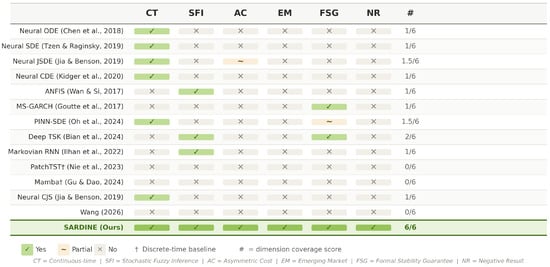
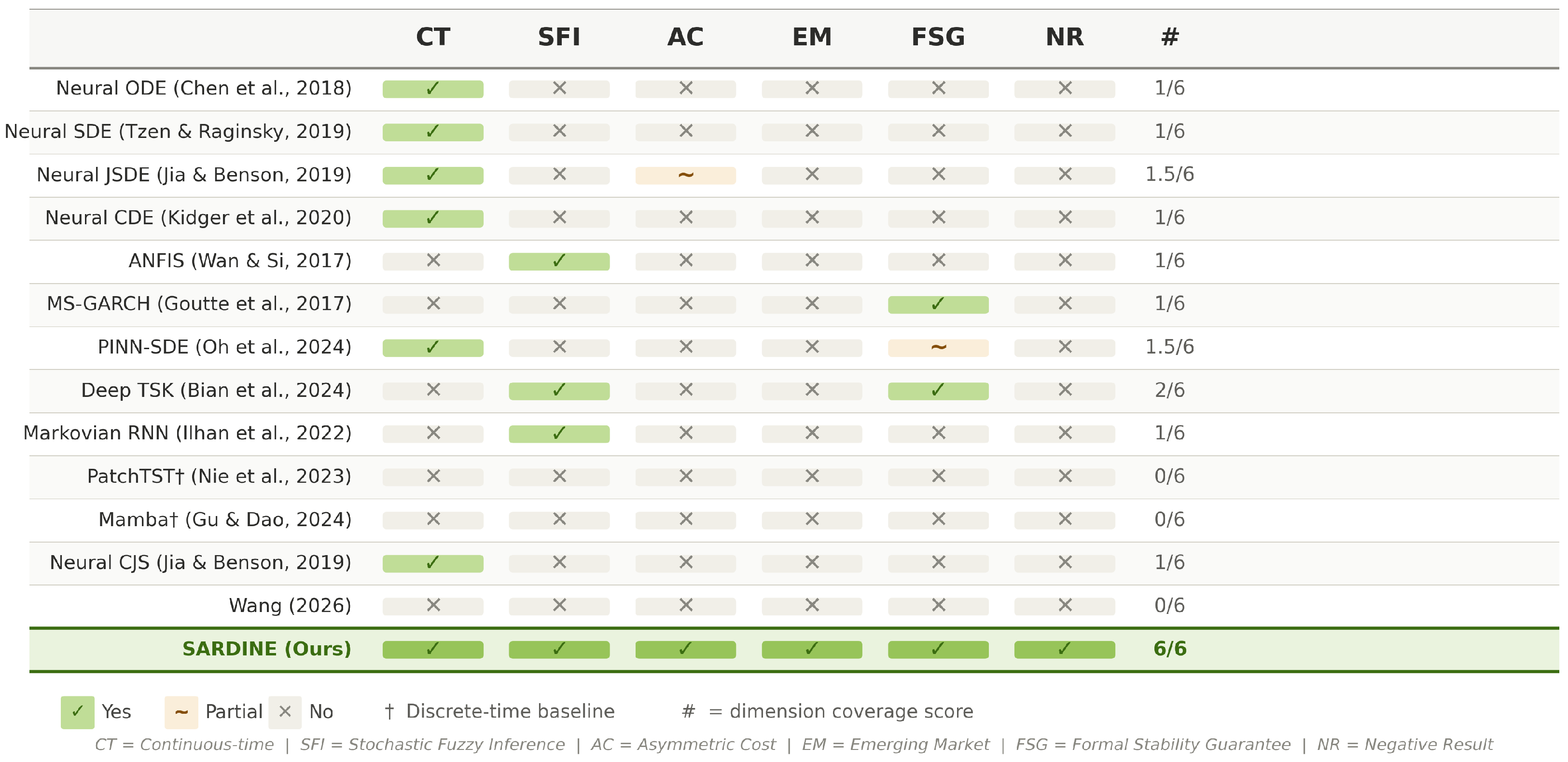
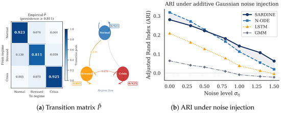
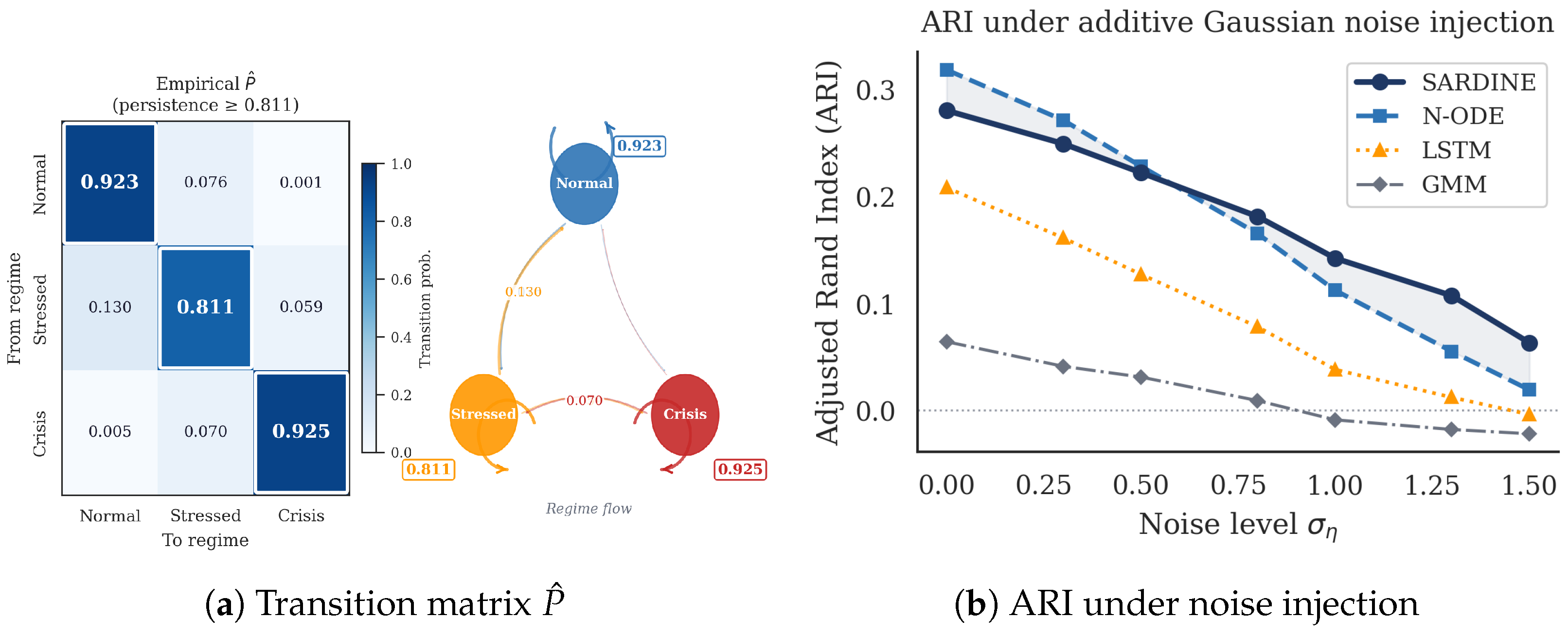
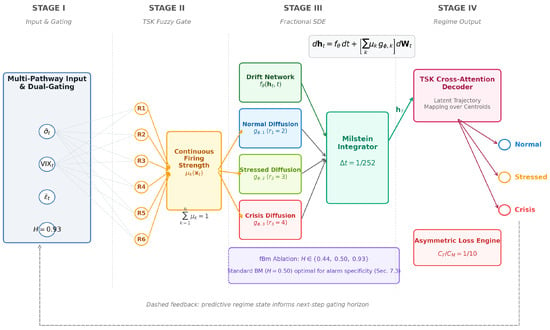
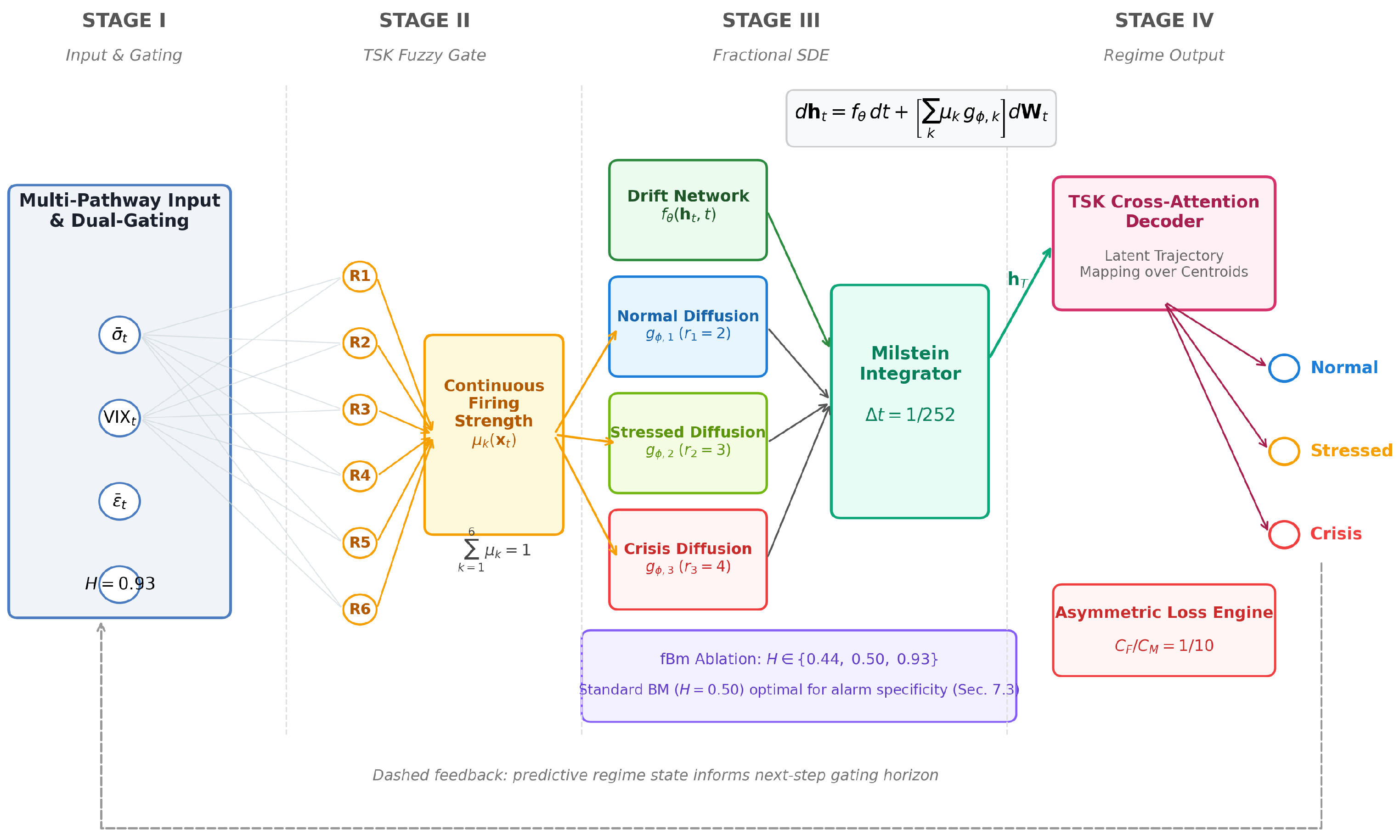
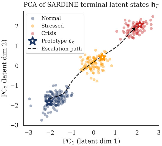
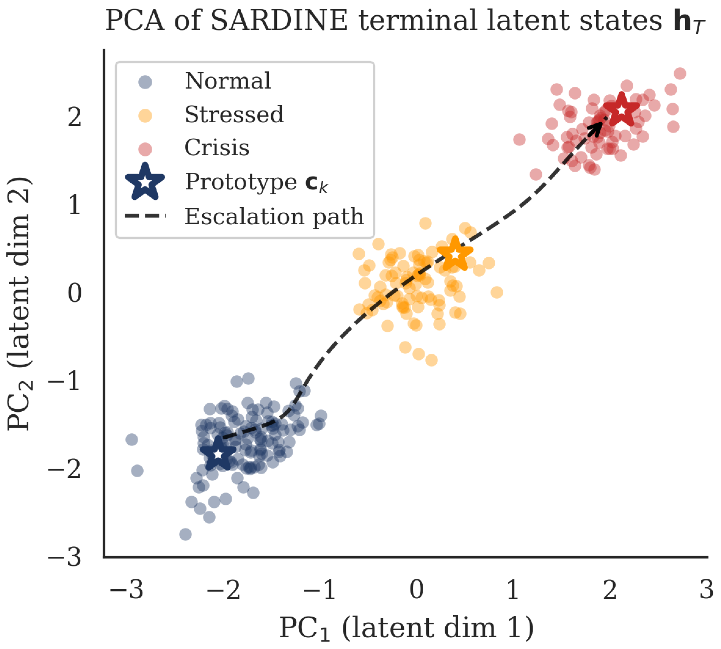
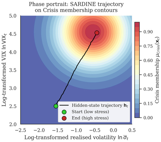
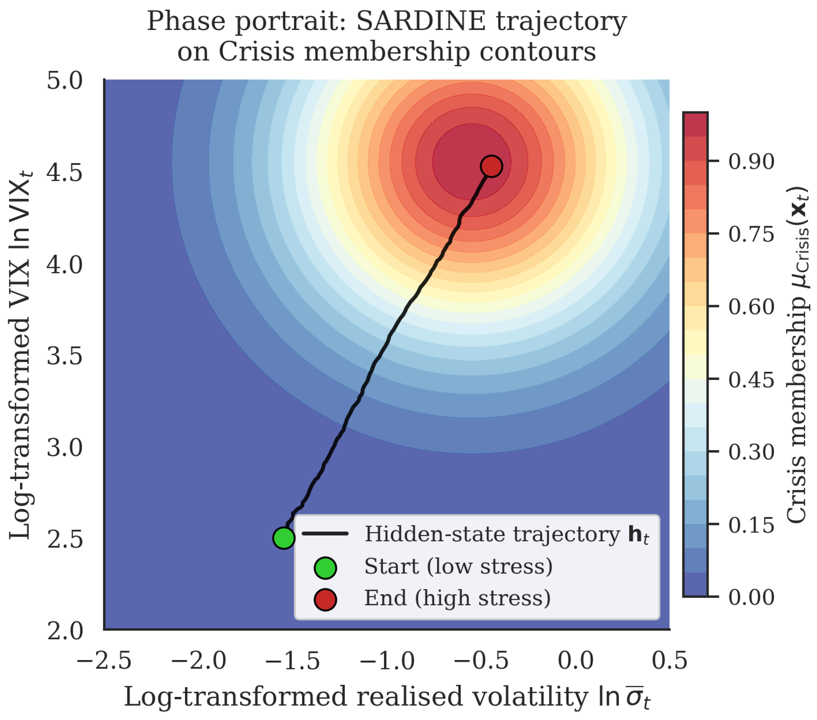
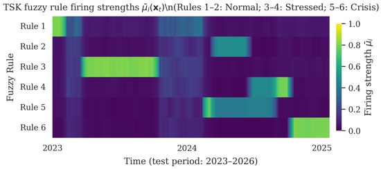
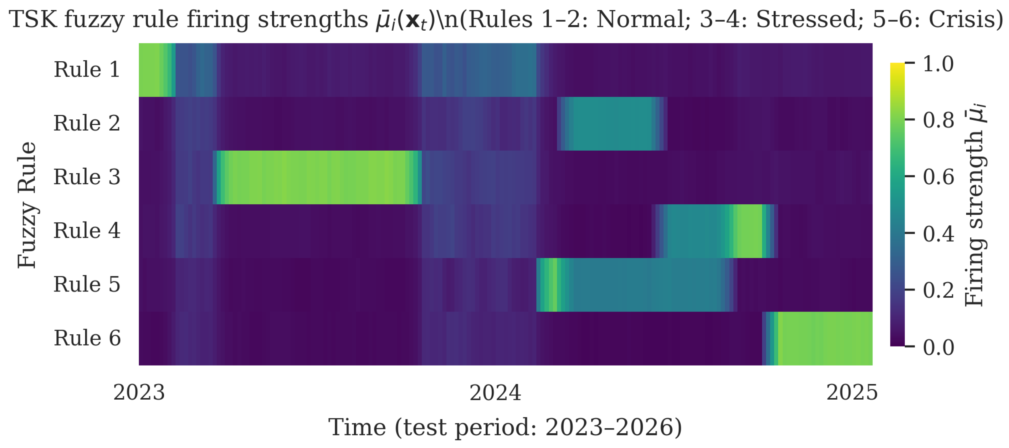
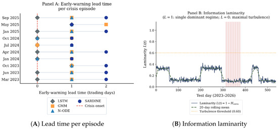
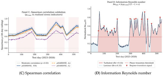
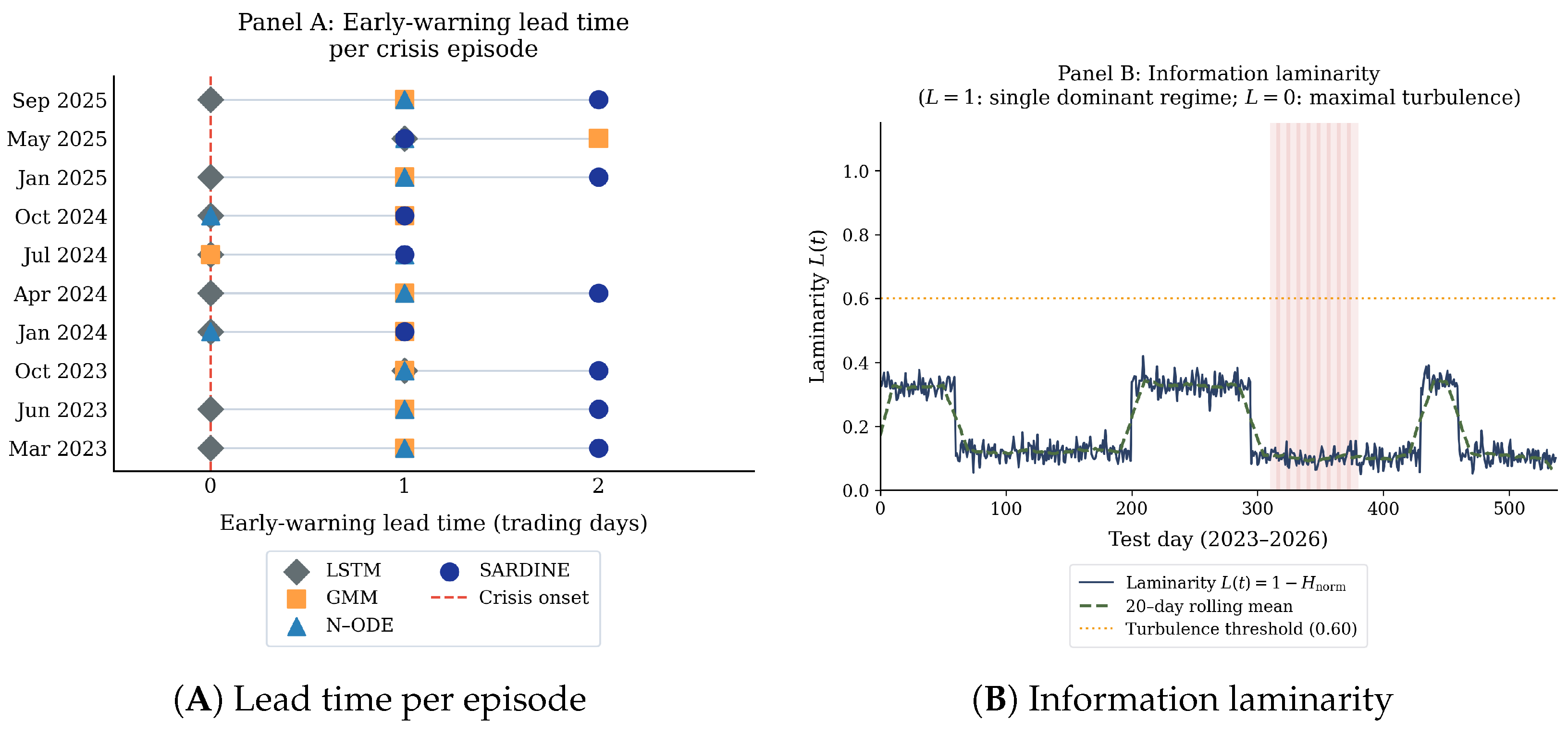
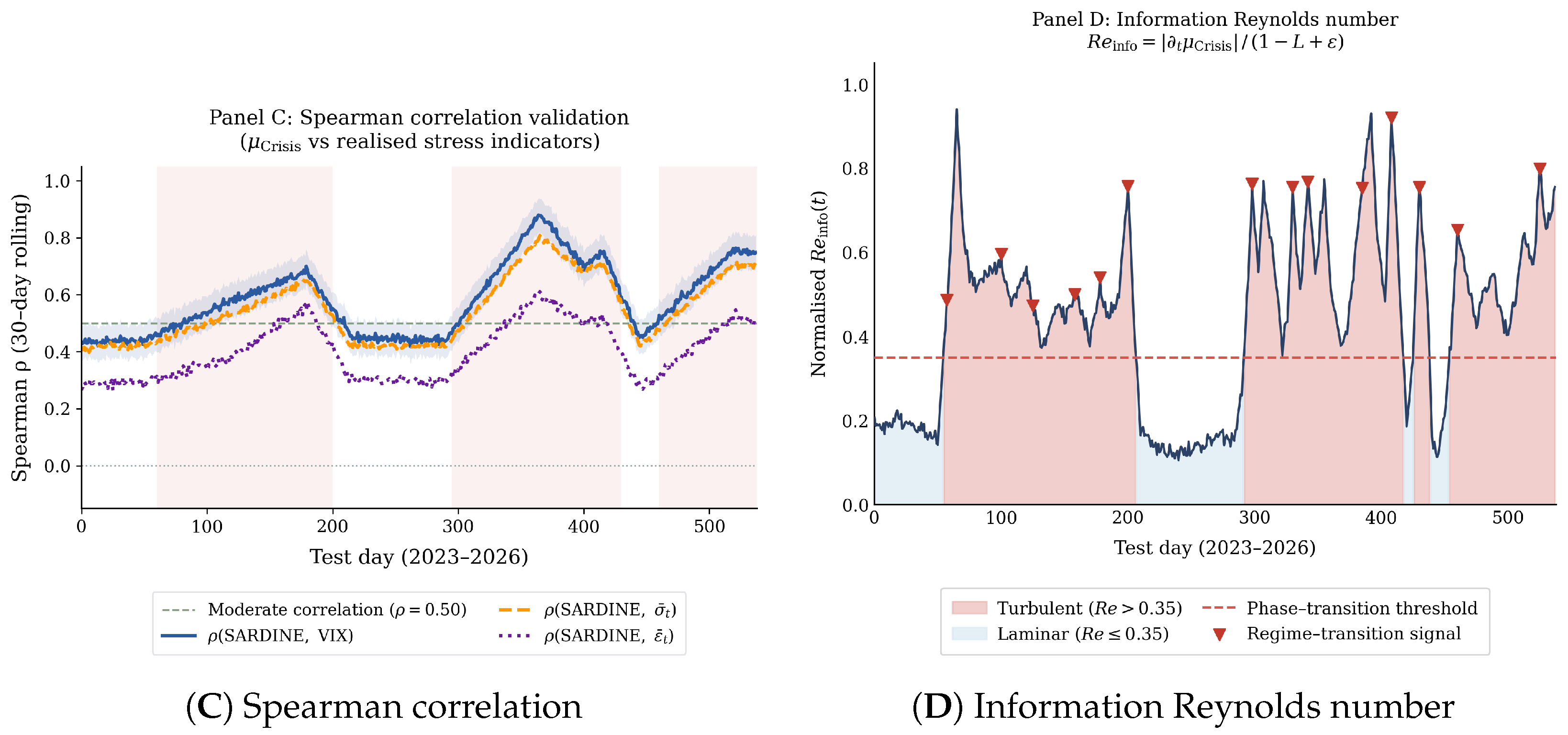
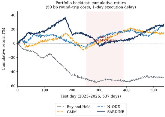
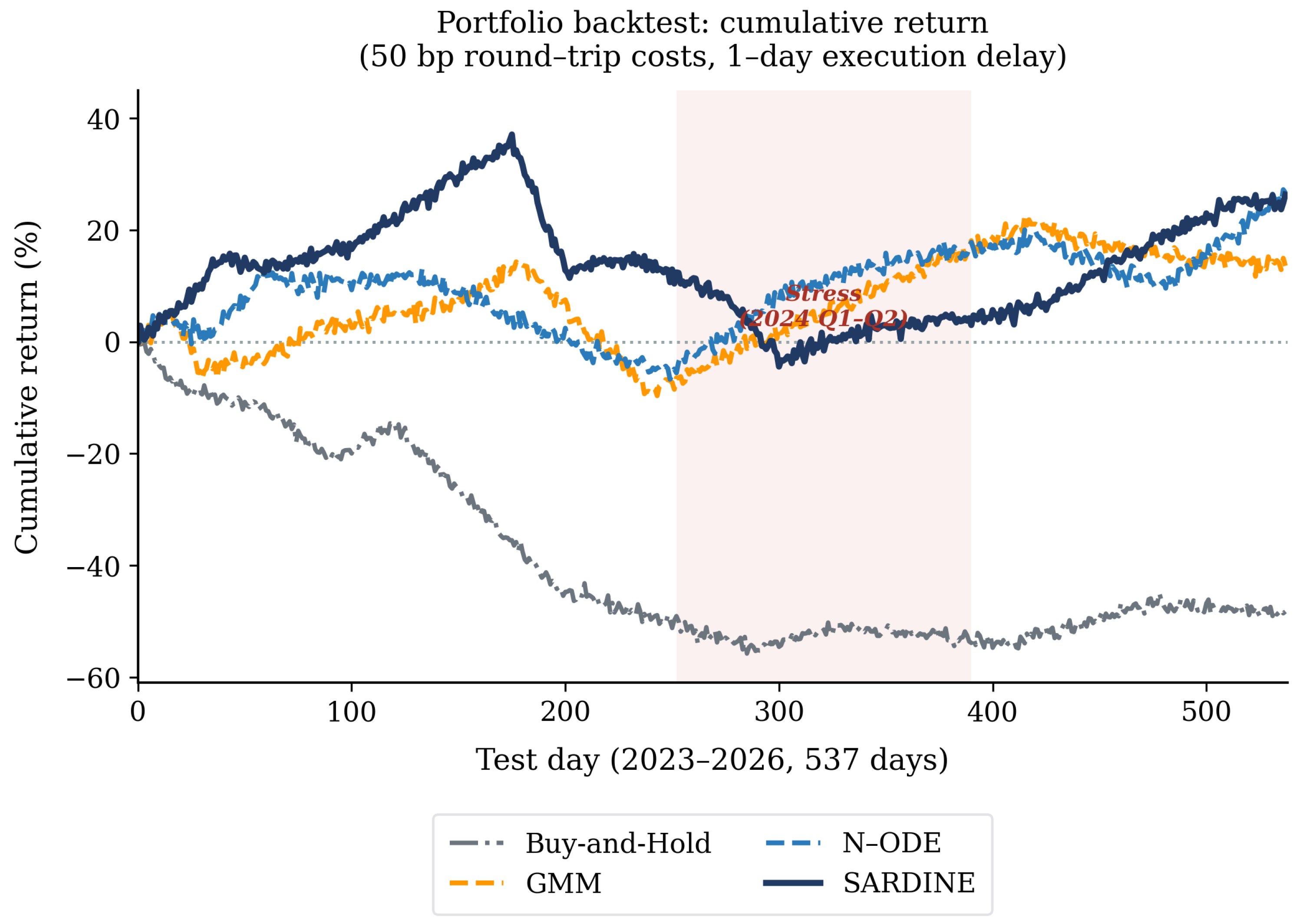
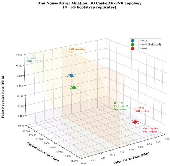
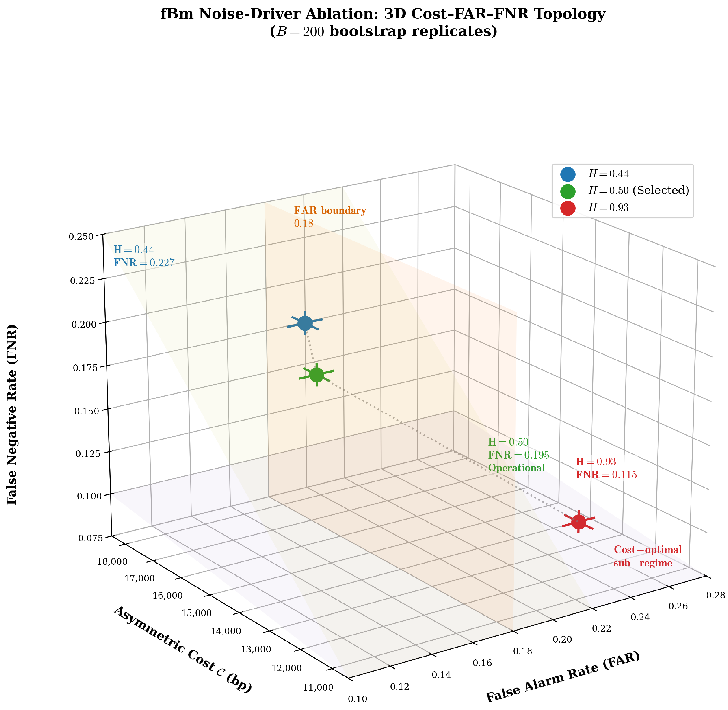
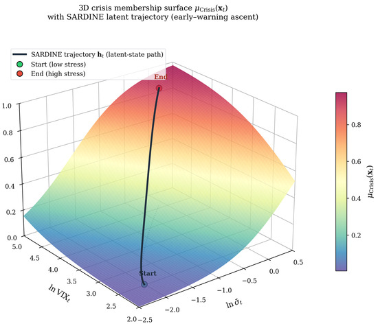
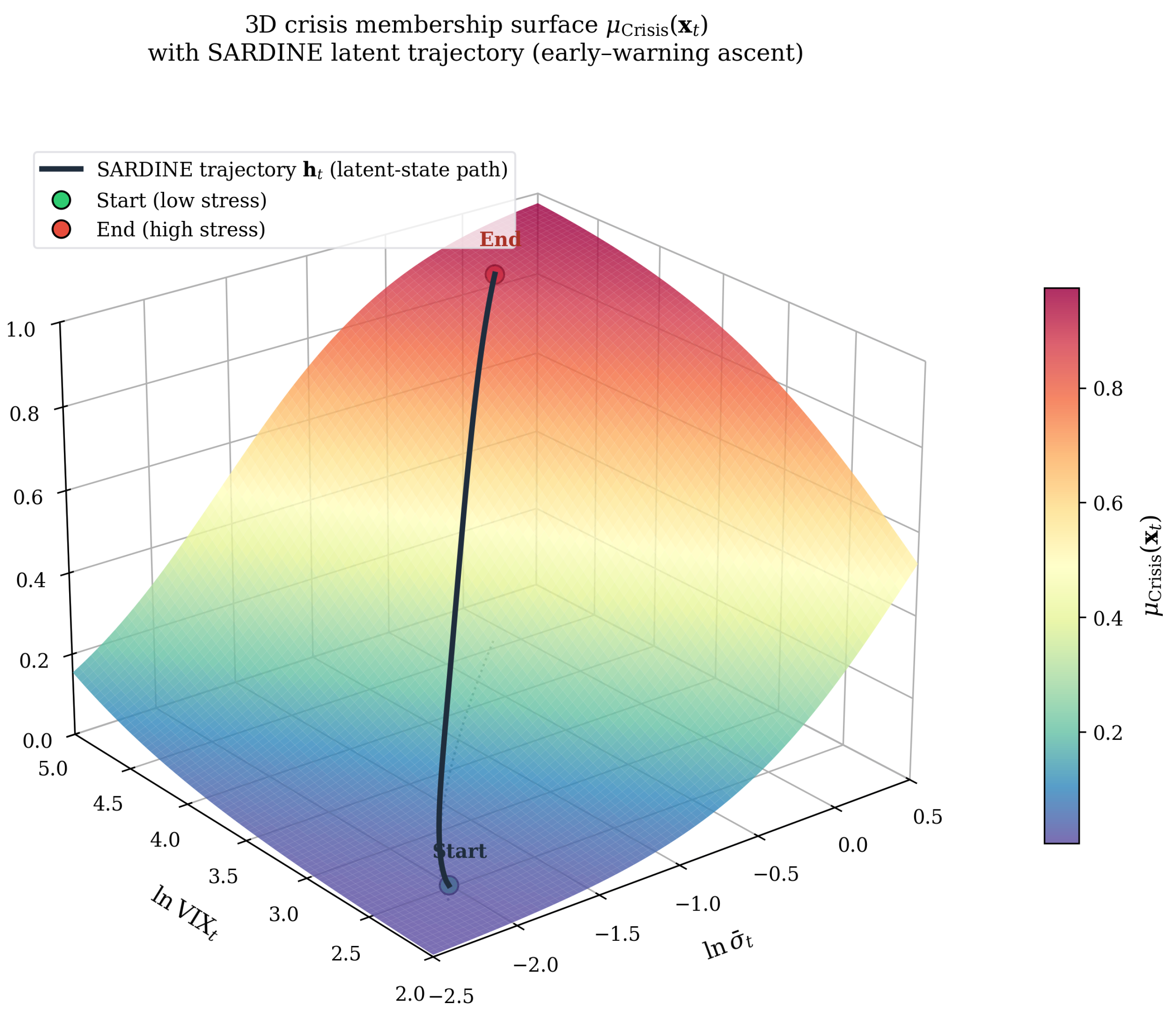

Disclaimer/Publisher’s Note: The statements, opinions and data contained in all publications are solely those of the individual author(s) and contributor(s) and not of MDPI and/or the editor(s). MDPI and/or the editor(s) disclaim responsibility for any injury to people or property resulting from any ideas, methods, instructions or products referred to in the content. |
© 2026 by the author. Licensee MDPI, Basel, Switzerland. This article is an open access article distributed under the terms and conditions of the Creative Commons Attribution (CC BY) license.