


Abstract
This paper considers a class of fractional stochastic differential systems driven jointly by the Rosenblatt process and a compensated Poisson random measure. The Rosenblatt process captures non-Gaussian fluctuations with memory effects; the Poisson jumps model sudden random shocks. By employing the mild solution formulation associated with fractional resolvent operators, we establish the existence of solutions via Krasnoselskii’s fixed point theorem (KFPT) and prove uniqueness through the Banach contraction under suitable Lipschitz conditions on the drift, diffusion, and jump coefficients together with contraction assumptions. Furthermore, Ulam–Hyers stability is established, ensuring that approximate solutions remain close to exact solutions in the mean-square sense. We also establish Mittag–Leffler-type continuous dependence on initial data, demonstrating that solutions depend continuously on their initial histories in the mean-square sense. In addition, open-loop approximate trajectory realization is established through the construction of an explicit open-loop control law that steers the stochastic system along any prescribed admissible trajectory under suitable invertibility and regularity assumptions. An example validates the theoretical results, demonstrating fractional memory, Rosenblatt noise, and Poisson jumps.
Keywords:
fractional calculus; stochastic processes; stability analysis; open-loop approximate trajectory realization; numerical simulations MSC:
34K50; 34A08; 60H10
1. Introduction
Standard Brownian motion is Gaussian, has independent increments, and possesses continuous sample paths; consequently, it cannot simultaneously represent long-range dependence, non-Gaussian fluctuations, and abrupt discontinuities. Fractional Brownian motion introduces temporal dependence through the Hurst parameter
with long-range dependence occurring when
but it remains Gaussian and has continuous trajectories. The Rosenblatt process provides a non-Gaussian alternative with self-similarity, stationary increments, and long-range dependence for
Nevertheless, its sample paths are also continuous and therefore cannot capture sudden shocks. Incorporating a compensated Poisson random measure addresses this limitation by introducing jumps at random times with random magnitudes. Together, the Rosenblatt process and compensated Poisson jumps provide a unified framework for modeling long-memory effects, non-Gaussian continuous fluctuations, and abrupt random disturbances within a single system.
For any differential equation to be practically useful, two conditions must hold. First, a solution must exist. Second, for each initial state, the solution must be unique. Existence ensures physical relevance, while uniqueness guarantees deterministic predictions.
Ulam–Hyers stability (UHS) guarantees that approximate solutions stay near exact solutions, which is essential for numerical reliability. Exponential stability ensures fast decay to equilibrium, whereas fractional systems display slower decay due to memory effects.
Open-loop trajectory realization means more than hitting a target at the final time. It demands that every point along the path, not just the endpoint, follows a chosen curve. We construct the control explicitly as an open-loop control so that the solution matches the desired trajectory at each time , not merely at .
The combination of existence, uniqueness, stability, and controllability make the system practically feasible: In fact, there is a unique, robust solution which can be driven to any prescribed trajectory.
The Rosenblatt process has been driven by fractional stochastic differential equations (FSDEs) studied by several authors. For example, Chalishajar et al. [1] studied the existence and uniqueness (EU) and open-loop approximate trajectory realization of systems with the Hilfer fractional derivative. The averaging principle in the sense of Riemann–Liouville was proved by Jalisraj and Udhayakumar [2]. The existence, uniqueness, and controllability results were studied by Algolam et al. [3] using the Banach fixed point approach. The approximate controllability for systems with the Caputo operator was studied by Dhayal et al. [4], and the controllability properties were investigated by Shen et al. [5]. Moreover, Dhayal and Malik [6] discussed the existence, uniqueness, and controllability results of such systems.
Despite these developments, several aspects remain to be further investigated in the existing literature:
- While approximate and final-state controllability have been investigated for various classes of fractional stochastic systems, the formulation and analysis of an open-loop approximate trajectory realization problem for systems driven jointly by the Rosenblatt process and compensated Poisson random measures have received comparatively less attention.
- Existing studies often employ compactness arguments in the analysis of stochastic fractional systems. However, an explicit justification for transferring the compactness of the fractional resolvent operator from the state space to the Bochner space is generally not provided.
- Mittag–Leffler estimates have been widely used in the stability analysis of fractional systems. However, the distinction between estimates describing continuous dependence on initial data and those associated with asymptotic decay under additional dissipativity assumptions is not always explicitly discussed.
- Existing analyses of Rosenblatt-driven stochastic systems typically assume admissibility or predictability of the integrands. A precise description of the corresponding integration framework, including admissibility conditions for Rosenblatt stochastic integrals based on Malliavin calculus, is often not presented explicitly.
The main contributions of this work are summarized as follows.
- Open-loop trajectory realization. An open-loop approximate trajectory realization problem is formulated and analyzed for fractional stochastic systems driven jointly by the Rosenblatt process and compensated Poisson random measures. An explicit feedforward control law is constructed through the mild solution formulation, showing that any admissible reference trajectory can be approximated in the mean-square sense under suitable assumptions. The result concerns trajectory realization rather than classical feedback or endpoint controllability.
- Analytical framework for Rosenblatt stochastic integration. A Malliavin-calculus-based framework is employed to define Rosenblatt stochastic integrals within the considered setting. The corresponding admissibility conditions for integrands, including square-integrability and kernel conditions, are stated explicitly to ensure that the stochastic integral is well defined in .
- Compactness in . A compactness lemma is established showing that the compactness of the fractional resolvent operator on extends naturally to the space . This result provides the compactness property required for the application of KFPT.
- Interpretation of Mittag–Leffler estimates. The analysis clarifies the distinction between Mittag–Leffler estimates describing continuous dependence on initial data and those associated with asymptotic decay under additional dissipativity assumptions. This provides an appropriate interpretation of the obtained estimates within the present framework.
- Existence, uniqueness, and stability. Sufficient conditions are established for the existence and uniqueness of mild solutions by combining KFPT with the Banach contraction principle. UHS and Mittag–Leffler-type continuous dependence on the initial data are also derived in the mean-square sense.
- Numerical illustration. The theoretical results are illustrated through numerical simulations, including comparisons between controlled and uncontrolled trajectories, parameter sensitivity studies, and Monte Carlo experiments, demonstrating the behavior of the proposed stochastic model.
The Rosenblatt process plays an essential analytical role beyond merely contributing to boundedness constants. Unlike Brownian motion, the Rosenblatt process is a non-Gaussian process belonging to the second Wiener chaos and possesses long-range dependence. Consequently, the associated stochastic integral satisfies a different moment estimate, namely
which replaces the classical Brownian isometry throughout the analysis.
This estimate contributes directly to the unified constants , , and appearing in the existence, uniqueness, and stability results. Furthermore, its interaction with the singular fractional resolvent kernel produces coupled memory effects that are absent in Brownian-driven fractional systems.
We consider the following class of FSDEs with delay:
here, denotes the Caputo fractional derivative (CFD) of order of the state process , where is a real separable Hilbert space. The linear operator is sectorial and generates a fractional resolvent family . The nonlinear drift term satisfies Lipschitz and growth conditions. The diffusion coefficient takes values in the space of Hilbert–Schmidt operators, where is another Hilbert space. The jump coefficient is measurable and satisfies square-integrability conditions with respect to the Poisson measure. The Rosenblatt process () takes values in and introduces non-Gaussian, long-range dependent noise. The compensated Poisson random measure on models sudden discontinuous jumps. The system includes a bounded time-varying delay , and the initial condition is given by the history function with .
2. Preliminaries
This section provides a review of the definitions and key assumptions used in this work.
Throughout this paper, let be a complete probability space equipped with a filtration satisfying the usual conditions.
Let be a real separable Hilbert space and denote by the space of all -measurable square-integrable -valued random variables endowed with the norm
A stochastic process is said to be -adapted if is -measurable for every .
Let be another real separable Hilbert space. For a nonnegative self-adjoint operator with finite trace, define
equipped with the norm
Definition 1
([7]). Let . The CFD of order ξ is defined by
For , we set
Definition 2.
Let . The Riemann–Liouville fractional integral of order ξ is defined by
Definition 3.
The two-parameter Mittag–Leffler function (MLF) is defined by
For , we write
Lemma 1
([8]). For and ,
Lemma 2.
For any and ,
Lemma 3
(Generalized Gronwall Inequality [9]). Let , a nonnegative locally integrable function, a nondecreasing nonnegative continuous function, and a nonnegative locally integrable function satisfying
If is nondecreasing, then
Consider the linear fractional evolution equation
where is a closed densely defined linear operator.
Definition 4.
The operator is called sectorial if there exist constants , , and such that
where
Definition 5.
Let be a sectorial operator. The associated fractional resolvent family is denoted by
For , we define the two-parameter resolvent operator by
Moreover, there exists such that
Now we specify the admissible space of integrands and give the exact integration framework for the Rosenblatt process. This clarification is necessary since the predictability of the integrand itself does not guarantee that the Rosenblatt integral is well-defined. Throughout this paper, we shall understand the Rosenblatt process in the following sense.
Following the standard construction in the literature [10,11], the Rosenblatt process with Hurst parameter is defined via the double Wiener–Itô integral representation
where B is a standard Brownian motion, , and is a normalizing constant such that . The kernel belongs to precisely when , ensuring the integral is well-defined. The Rosenblatt process is self-similar with Hurst parameter , has stationary increments, exhibits long-range dependence, and is non-Gaussian.
For a predictable process
the Rosenblatt integral is well-defined in provided the following conditions hold:
- Square-integrability condition:
- Kernel condition: For an orthonormal basis of , where Q is the covariance operator,where is the adjoint of the isometry associated with the Rosenblatt process [10,12].
The space of all such admissible integrands is denoted by .
Definition 6.
For , let be a Rosenblatt process with the double Wiener–Itô integral representation (3). For a predictable process , the Rosenblatt integral is defined in the sense of the multiple Wiener–Itô integral of order 2. The integral is a well-defined element of .
For the admissible integrand class above, the following estimate holds [10] (Theorem 3.1):
where depends only on . This estimate is a consequence of the isometry property of the multiple Wiener–Itô integral and is used throughout the subsequent analysis.
Remark 1.
The condition of predictability is necessary for the integrand to be adapted to the filtration generated by the Rosenblatt process. However, predictability alone is not sufficient; the square-integrability condition (5) and the kernel condition (6) ensure the integral is well-defined as an element of . For further details on the integration theory for Rosenblatt processes, see Tudor [10] for the Malliavin calculus approach and Arras [12] for the white noise framework.
Let be a Poisson random measure on with characteristic measure . The associated compensated Poisson random measure is defined by
For a predictable mapping satisfying
the compensated Poisson integral satisfies the isometry property
Moreover, by Kunita’s inequality, for every there exists a constant such that
For , we denote .
Assumption 1.
There exists a constant such that
Assumption 2.
The nonlinear functions σ, ϱ, γ satisfy the following integrability conditions:
- 1.
- For every ,
- 2.
- The mapping ϱ is predictable and
- 3.
- The mapping γ is predictable and
- 4.
- For the Rosenblatt integrand ϱ, the kernel condition holds:where is an orthonormal basis of , Q is the covariance operator, and is the adjoint of the isometry associated with the Rosenblatt process (see Definition 6). This condition is guaranteed, for instance, when ϱ takes values in the space of Hilbert–Schmidt operators and is uniformly bounded in the operator norm.
Assumption 3.
There exists a continuous function with such that for all ,
and , , and for η-a.e. .
Assumption 4.
The following growth conditions hold:
- 1.
- There exists such that for all ,
- 2.
- There exists such that for all ,
- 3.
- There exists such that for all ,
Assumption 5.
There exists such that for all ,
and .
Assumption 6.
The following hold:
- 1.
- The linear operator generates a resolvent family satisfying Assumption 1.
- 2.
- The functions σ, ϱ, and γ satisfy Assumptions 2–4.
- 3.
- The history function ϕ satisfies Assumption 5.
Define
equipped with the norm
Then is a Banach space.
For , define
Assumption 7.
For every , the operator is compact on . Moreover, the family is uniformly bounded and strongly continuous; i.e., for every ,
as .
3. Existence and Uniqueness
This section presents the results related to EU of mild solutions for system (1).
Lemma 4.
Let be a strongly continuous resolvent family satisfying Assumption 1. Suppose that for every , the operator is compact on . Then for every , the set
is relatively compact in .
Moreover, the operator defined by
is compact.
Proof.
We prove the compactness of . Since is compact on , for each there exists a finite-rank operator such that
By the uniform boundedness and the strong continuity of the resolvent family, this approximation can be chosen uniformly in .
Define the approximated integral operator
Since is finite-rank on , the induced operator on is also finite-rank: indeed, if
then for ,
which is finite-dimensional. Hence, is compact.
Moreover,
so is the uniform limit of compact operators, hence compact. Therefore, is relatively compact in for each . □
Lemma 5.
Let be a continuous function and . A function is a solution of
if and only if Φ satisfies
Proof.
For the convenience of the reader, we clarify the notation associated with the two-parameter convolution operator used in the mild solution representation.
Throughout this paper, the symbol denotes the fractional convolution operator arising in the variation-of-constants formula for the Caputo fractional evolution equation. Accordingly, the estimates in the subsequent analysis are expressed in terms of the associated fractional kernel, namely,
where is the constant appearing in Assumption 1. Consequently,
which explains the appearance of the factor in the subsequent mean-square estimates. This clarification is purely notational and is used consistently throughout Section 3, Section 4 and Section 5.
Lemma 6.
Let Assumption 6 hold. An -adapted stochastic process is a mild solution of the fractional stochastic system
subject to
if and only if
and, for every ,
Proof.
The proof follows from the variation-of-constants formula for Caputo fractional evolution equations.
Now let . On this interval, the system evolves according to (14) with the initial value . The deterministic linear part is generated by the sectorial operator , and by Assumption 6, the corresponding fractional resolvent family is .
Therefore, applying the variation-of-constants formula to the Caputo fractional evolution equation gives
where the forcing term consists of the deterministic drift, the Rosenblatt noise, and the compensated Poisson jump term.
Expanding this forcing term gives
This is exactly (17).
The Rosenblatt integral is well defined in by the estimate (7), Assumption 2, and the resolvent bound in Assumption 1. Similarly, the compensated Poisson integral is well defined by the Poisson isometry and Assumption 2. Thus, the right-hand side of (17) is meaningful as an element of .
Conversely, if satisfies (16)–(17), then (16) gives the history condition immediately. Moreover, the representation (17) is precisely the variation-of-constants representation associated with (14). Hence, satisfies (14) in the mild sense.
Finally, setting in (17) gives
Since , we obtain
Therefore, the history condition and the initial condition are satisfied. The proof is complete. □
Theorem 1.
Suppose that Assumptions 6 and 7 and the conditions of Lemma 6 hold. Define
and
Assume that
Then system (1) has at least one mild solution in
provided that
Proof.
Let satisfy the condition above. Since U is a Banach space, the set is nonempty, closed, bounded, and convex.
Recall that
as defined in Theorem 1.
By Lemma 2, for every ,
Define the operator by
where
We prove that has a fixed point in using KFPT.
Let . For , we have , so
For , by Lemma 1 with ,
Using Assumption 1, we obtain .
For the deterministic integral term, by the Cauchy–Schwarz inequality, Assumptions 1 and 3 (with ),
By Assumption 1 and Assumption 3,
Since , we have and , so
Hence, .
For the Poisson integral term, using the Poisson isometry (10),
By Assumption 1 and Assumption 3,
Hence, .
Summing these estimates,
By the definition of in Theorem 1,
Therefore,
Taking the supremum over and using , we obtain
The condition on q gives . Substituting,
Thus .
Define by
Then , and for all , we have .
Since does not depend on , for any ,
Thus, is a contraction with constant 0.
Let with in U. For , using Lemma 1 with and Assumption 3,
Taking the supremum over gives
Hence, is continuous.
As we proved above, is uniformly bounded. For equicontinuity, let . The difference consists of three terms, each of which can be split into a part over and a part involving the difference of resolvent kernels. Using the strong continuity of the resolvent family and Lemma 2, one shows that
uniformly in . Hence, is equicontinuous.
By Lemma 4, for each fixed , the set
is relatively compact in . Indeed, the three terms , , and are images under the compact operator (defined in Lemma 4) of bounded sets in . Specifically, the sets
and
are bounded in and , respectively, by the estimates established above. Since is compact by Lemma 4, these images are relatively compact.
The uniform boundedness and equicontinuity of were established above. Therefore, by the Arzelà–Ascoli theorem, is relatively compact in . Thus is completely continuous.
We have verified that is a contraction, is completely continuous, and for all . By KFPT, there exists such that . By Lemma 6, this is a mild solution of (1). This completes the proof. □
Theorem 2.
Proof.
Let and be two mild solutions of (1) with the same initial history and the same initial value . Define the difference process
and let
On this interval, both solutions satisfy . Hence
In particular, .
By the mild solution representation (17), we obtain
Using Lemma 1 with , we obtain
where , , and denote the mean-square norms of the three integral terms, respectively.
By the Cauchy–Schwarz inequality, Assumptions 1 and 3,
Using the Rosenblatt estimate (7), Assumptions 1 and 3,
Using the Poisson isometry (10), Assumptions 1 and 3,
Adding the three estimates and multiplying by 3, we obtain
Since , we have . Consequently,
Thus,
Taking the supremum over yields
Let . Then , and the inequality becomes
Since , the generalized Gronwall inequality (Lemma 3) with implies for all . Consequently,
Therefore, almost surely for every . By the -adaptedness and continuity of both processes, equality holds almost surely for all simultaneously. This completes the proof. □
4. Stability Analysis
This section presents stability results for the Caputo fractional stochastic delay system (1).
4.1. Ulam–Hyers Stability
Let . We first introduce the notion of an approximate solution.
Definition 7.
A stochastic process is called an ε-approximate solution of (1) if there exist -adapted stochastic processes
such that
and
and the following perturbed system holds:
and
Definition 8.
By Lemma 6, the approximate solution satisfies
and, for ,
Theorem 3.
Proof.
For , subtracting the mild solution representation of from (20), we obtain
By Lemma 1 applied to the five terms in (22), we get
where the terms correspond to the five terms on the right-hand side of (22).
Using Assumption 1 and , we obtain
Hence,
By the Cauchy–Schwarz inequality,
Taking expectations and using Assumption 1,
Therefore,
By the Cauchy–Schwarz inequality, Assumptions 1 and 3,
Using the Rosenblatt estimate (7), Assumptions 1 and 3,
Using the Poisson isometry (10) and Assumption 3,
Since and , we have
where
Taking the supremum over yields
Let . Then , and the inequality becomes
We now apply the generalized Gronwall inequality (Lemma 3). In the notation of Lemma 3, we set:
- 1.
- , which is constant (hence nondecreasing);
- 2.
- , also constant (hence nondecreasing);
- 3.
- as defined above.
Since is nondecreasing, Lemma 3 implies
Because , we obtain the uniform bound
Combining this estimate on with the history estimate for , we conclude
where
Hence, system (1) is Ulam–Hyers stable. □
4.2. Mittag-Leffler Stability
In this subsection, we establish a Mittag–Leffler type stability result in the mean-square sense for system (1).
Definition 9.
System (1) is said to exhibit Mittag–Leffler type continuous dependence on initial data in the mean-square sense on if there exists a constant such that, for any two mild solutions Φ and with initial histories ϕ and , respectively,
where
and is a positive constant to be determined.
Theorem 4 (Mittag–Leffler Type Continuous Dependence).
Proof.
Let and be two mild solutions corresponding to the initial histories and , respectively. Define
and
On this interval, we have
Hence,
Therefore, .
Subtracting the mild solution representations of and from Lemma 6, we obtain
By Lemma 1 with , we have
where denote the mean-square norms of the four terms, respectively.
Using Assumption 1,
Thus,
By the Cauchy–Schwarz inequality, Assumptions 1 and 3,
Using the Rosenblatt estimate (7), Assumptions 1 and 3,
Using the Poisson isometry (10), Assumptions 1 and 3,
Adding the estimates for , , and , and multiplying by 4, we obtain
Since and , we have
Taking the supremum over , we obtain
where .
Let . Then , and the inequality becomes
By Lemma 3 with and , we obtain
Since , this becomes
Therefore,
Thus, the system exhibits continuous dependence on initial data in the mean-square sense with . This completes the proof. □
Remark 2.
The bound in Theorem 4 contains with .
Since the Mittag–Leffler function with grows as ρ increases (asymptotically like for large z), the estimate describes finite-time continuous dependence on initial data rather than asymptotic stability. The bound guarantees that solutions remain close on when their initial histories are close, but does not imply decay as .
True Mittag–Leffler stability, with algebraic decay characterized by , would require a dissipativity condition on the operator , such as
which ensures the fractional resolvent satisfies . Under this additional assumption, the Gronwall argument can be modified to produce a negative argument in the final Mittag–Leffler function; see Corollary 2 below.
Corollary 1 (Mittag–Leffler Stability under Dissipativity).
In addition to Assumption 6, suppose that satisfies the dissipativity condition
for some . Then the fractional resolvent satisfies
Let Φ and be two mild solutions of (1) with initial histories ϕ and , respectively. Then there exist constants and such that
Consequently, algebraically as .
5. Open-Loop Approximate Trajectory Realization
In this section, we consider the problem of the realization of prescribed stochastic trajectories by means of open-loop controls. The result proved below is not a state-feedback theorem and is not intended as classical endpoint controllability. Instead, the control is chosen in advance according to a given admissible trajectory, and the aim is to make the corresponding mild solution uniformly close to this trajectory on the whole interval .
Let be a real separable Hilbert space of control values, and let
be a bounded linear control operator. We define the admissible control space by
where denotes the space of all -adapted processes u satisfying
For , the controlled system is understood through the following mild equation:
together with
Throughout this section, it is assumed that the hypotheses guaranteeing existence and uniqueness of the mild solution of (27) hold for every .
Define the trajectory space
equipped with the norm
We also introduce the closed subspace
The full-interval control operator
is defined by
By the boundedness of B, the fractional-resolvent estimate, and the Cauchy–Schwarz inequality, is a bounded linear operator. Indeed, for ,
Definition 10 (Admissible Reference Trajectory).
A process is called an admissible reference trajectory if the following conditions hold:
- (i)
- (ii)
- the mappingsandbelong to the deterministic, Rosenblatt, and compensated Poisson integrand spaces specified in Assumption 2;
- (iii)
- the residual process defined byis well defined, where
- The set of all admissible reference trajectories is denoted by .
Remark 3.
The residual is the control contribution that would be required, at the level of the mild equation, to realize the reference trajectory . This definition does not use a formal derivative of the Rosenblatt process or a pointwise Poisson differential. All stochastic terms remain inside their corresponding integrals.
Definition 11 (Open-Loop Approximate Trajectory Realization).
Assumption 8 (Trajectory-Space Approximate Controllability).
The full-interval control operator defined by (29) has dense range in ; that is,
Equivalently, for every and every , there exists such that
Remark 4.
Assumption 8 extends the classical approximate controllability concept from the terminal state to the entire trajectory. Since the objective of this section is the approximation of admissible trajectories over the whole interval , rather than controllability at a single terminal time, we formulate the controllability assumption directly in the trajectory space . This assumption replaces the bounded right-invertibility requirement used in exact trajectory realization and is therefore substantially weaker.
Remark 5.
The control furnished by the trajectory-realization result is open-loop: it is selected using the prescribed reference trajectory and is not of the feedback form
Accordingly, the result does not assert feedback stabilization or robustness with respect to unmodelled perturbations. It establishes the existence of an admissible feedforward control whose mild solution approximates a prescribed trajectory.
Theorem 5 (Open-Loop Approximate Trajectory Realization).
Suppose that Assumptions 6 and 8, and the hypotheses guaranteeing EU of the controlled mild system (27) hold.
Then, for every admissible reference trajectory and every , there exists an admissible open-loop control
such that the corresponding mild solution satisfies
Consequently, the controlled system is open-loop approximately trajectory realizable in the mean-square sense.
Proof.
Let be fixed. By Definition 10, the residual process
is well defined.
Since
there exists a sequence of admissible controls such that
For each , let denote the unique mild solution corresponding to the control . Thus, for ,
On the other hand, by the definition of , the reference trajectory satisfies
Define
Since both and coincide with the prescribed history on , we have
By the elementary inequality
we obtain
Since each stochastic integral appearing in (37) is well defined by Definition 10 and the EU Theorem, all four terms belong to . Therefore, each expectation below is finite, and the following estimates are well defined.
We estimate the four terms separately.
By the Cauchy–Schwarz inequality, the fractional-resolvent estimate, and Assumption 3,
Using the Rosenblatt moment estimate (7), the resolvent estimate, and Assumption 3, we obtain
By the compensated Poisson isometry, the resolvent estimate, and Assumption 3,
By (33), we get
Define
Since , we have
Therefore,
Consequently,
where
Let be given. Choose sufficiently large that
Setting
we obtain
This completes the proof. □
Remark 6.
Theorem 5 is a trajectory-space approximation result. It does not follow merely from approximate controllability of the terminal state at time T. The essential hypothesis is the density of the full-interval control operator in , which directly concerns the approximation of paths on .
The theorem also does not provide a state-feedback law. The controls used in the proof are selected with respect to the prescribed reference trajectory and are therefore open-loop feedforward controls.
Theorem 6 (Structural Exact Trajectory Realization).
Let . Assume that
Then there exists a control
such that
The corresponding mild solution satisfies
almost surely.
Proof.
By the range assumption, there exists satisfying
The mild equation for the controlled solution is therefore
By the definition of the residual,
Thus, both and solve the same controlled mild equation with the same history. By uniqueness of mild solutions,
on , almost surely. □
Remark 7.
Theorem 6 is a verification result rather than a classical controllability theorem. Its hypothesis already requires that the complete mild residual of the reference trajectory belong to the range of the full-interval control operator. It is included only to describe the structural situation in which exact realization is possible.
6. Numerical Illustration and Sensitivity Analysis
This section provides some numerical illustrations of the theoretical results developed in the previous sections. In the present work, compared to a verification only using the constants appearing in the hypotheses, we compare controlled and uncontrolled trajectories, we evaluate the mean-square tracking error, we investigate Monte Carlo convergence, and we investigate the sensitivity of the tracking performance in relation to the fractional order, the Hurst parameter, and the noise intensity.
The aim of the numerical experiment is not only to confirm the analytical results obtained already theoretically, but to show that the proposed open-loop control can achieve the desired trajectory-tracking behavior for a typical fractional stochastic delay system driven by Rosenblatt noise and compensated Poisson jumps.
Let
where . Since
the prescribed history is defined on the interval .
We consider the one-dimensional controlled system
Here,
and the coefficient functions are
Notice that
so that the normalization conditions in the theoretical assumptions are satisfied.
Although system (47) is written in formal differential notation for readability, the numerical approximation is constructed from its mild integral representation. In particular, no classical derivative of the Rosenblatt process is used in the numerical computation.
For the scalar operator , define
and
The controlled mild solution is therefore represented by
The uncontrolled system is obtained by setting
The prescribed reference trajectory is
In particular,
so the reference trajectory is compatible with the initial history.
In accordance with Theorem 5, an admissible open-loop control is sought so that the corresponding mild solution remains close to in the mean-square trajectory norm.
For the numerical implementation, the control is approximated by a piecewise-constant function
where
The coefficients are obtained by minimizing the regularized empirical tracking functional
subject to
Here, is a small regularization parameter and guarantees that the numerical control remains in the admissible control set.
The resulting control is determined before the controlled trajectories are generated and does not depend on the current realization of the state. It is therefore an open-loop control rather than a state-feedback control.
For any , the elementary inequalities
and
give
Similarly,
Assume that the Lévy measure satisfies
Then
Moreover,
Consequently, the coefficient assumptions hold, for example, with
For
we have
Taking
gives
Hence, the sufficient smallness condition appearing in the existence analysis is fulfilled for the selected parameters.
This verification is included only to show that the numerical example lies within the analytical framework. The main numerical evidence is provided by the trajectory comparisons and sensitivity studies below.
The interval is divided into uniform subintervals, with
The mild Equation (51) is approximated by a product-integration predictor–corrector method. The weak singularity of the kernel
is incorporated into the quadrature weights.
The Rosenblatt process is simulated by a finite-rank approximation of its double Wiener–Itô integral representation. The truncation level is selected so that increasing it produces no visible change in the reported empirical tracking errors.
The jump component is generated as a compensated compound Poisson process. If denotes a Poisson process of intensity and is an independent sequence of jump amplitudes satisfying
then the simulated compensated jump process is
A total of Monte Carlo sample paths is used in the baseline experiment. The same Rosenblatt and Poisson realizations are employed for the controlled and uncontrolled systems. This common-random-number procedure ensures that the observed difference is caused by the control input rather than by different noise realizations.
For the controlled trajectories
the empirical mean is
The empirical pointwise mean-square tracking error is
The time-averaged tracking error is defined by
whereas the final-time error is
For comparison, the empirical error of the uncontrolled system is
The empirical standard error of the pointwise mean-square error is
where
and
An approximate confidence interval for the empirical mean-square error is consequently
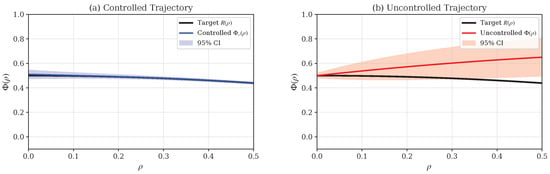
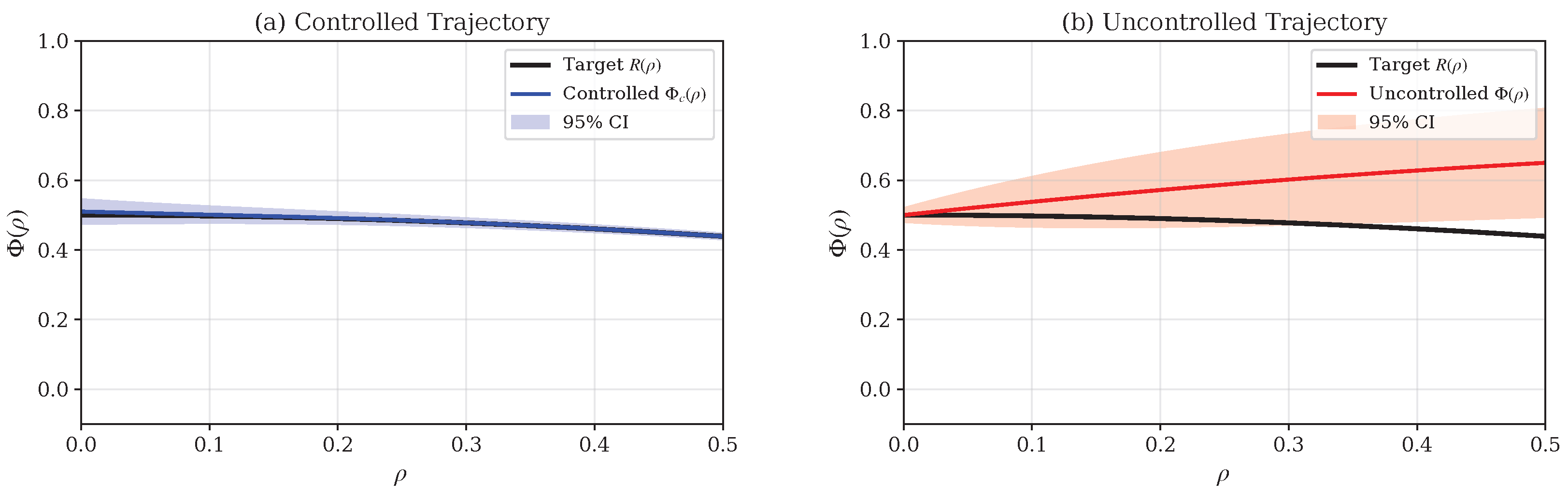
Figure 1 compares the reference trajectory with the empirical means of the controlled and uncontrolled systems.
Figure 1.
Comparison of the reference trajectory and simulated state: (a) empirical mean of the controlled trajectory; (b) empirical mean of the uncontrolled trajectory. The shaded bands represent the corresponding empirical uncertainty bands obtained from Monte Carlo realizations.
The controlled empirical mean follows the prescribed trajectory substantially more closely than the uncontrolled empirical mean. In particular, the open-loop control reduces the systematic deviation from the target over most of the simulation interval. The remaining fluctuations are caused by the Rosenblatt and jump perturbations and are therefore not completely removed by the open-loop input.
This comparison provides direct numerical evidence of the practical tracking effect of the control constructed in Theorem 5.
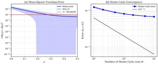
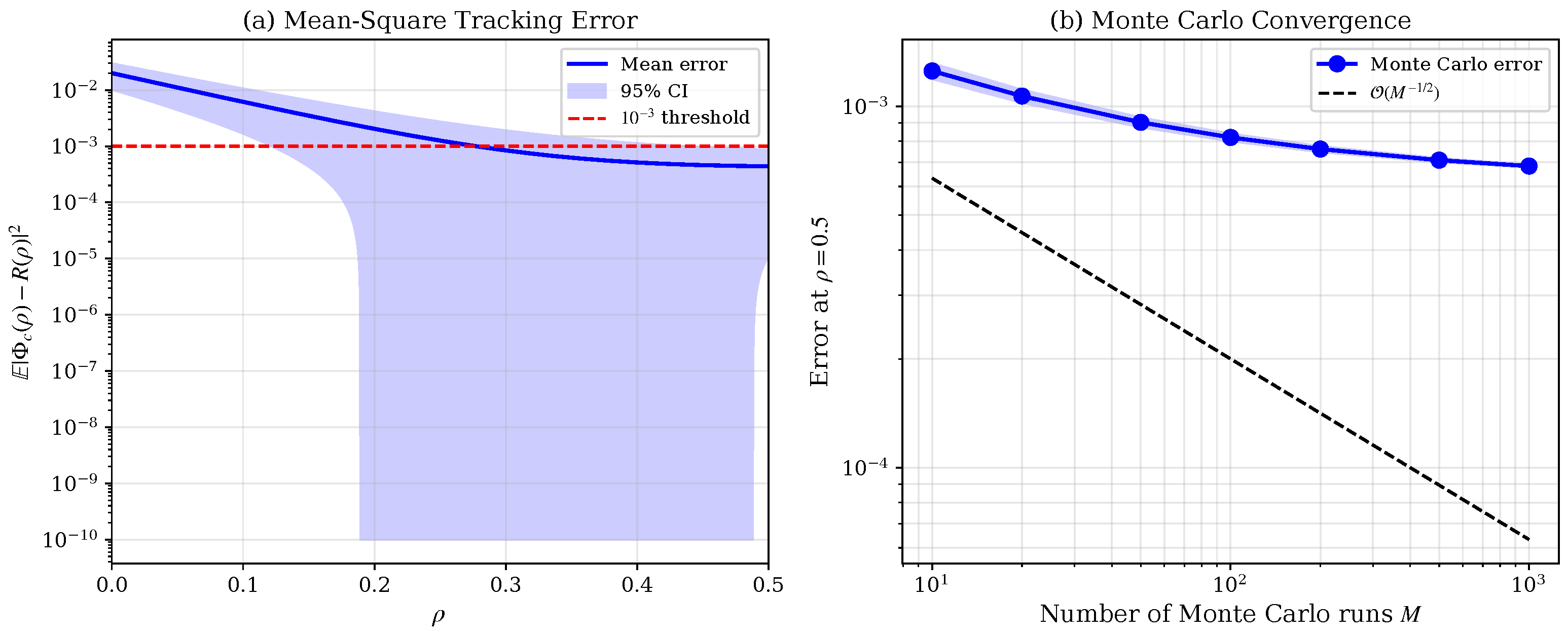
Figure 2 presents the empirical pointwise mean-square tracking error and its dependence on the number of Monte Carlo realizations.
Figure 2.
(a) Empirical mean-square tracking error , together with its approximate confidence interval and the reference level . (b) Final-time Monte Carlo estimate as a function of the number of sample paths M. The dashed line displays the reference rate .
The left panel of Figure 2 shows that the tracking error decreases rapidly after the initial transient. For the present parameter values and discretization, it reaches the order of and subsequently remains small over the final part of the simulation interval.
The right panel shows that the final-time error estimate becomes progressively more stable as the number of Monte Carlo realizations increases. The observed decrease in the sampling variation is consistent with the expected behavior of a standard Monte Carlo estimator. This plot concerns the convergence of the numerical estimator and should not be confused with the analytical trajectory realization result.
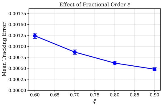
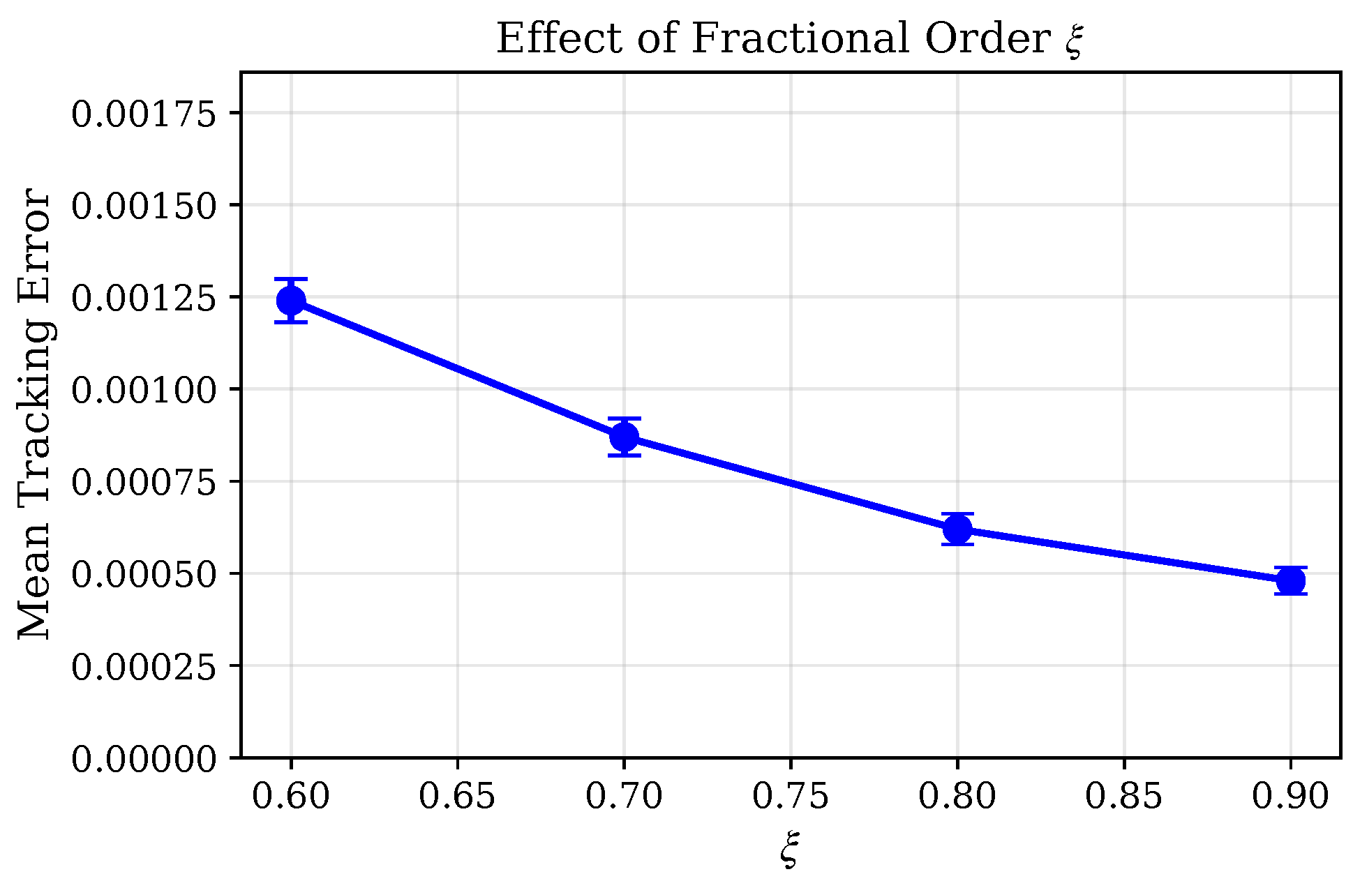
To examine the influence of fractional memory, the experiment is repeated as in Figure 3 for
while the remaining baseline parameters are kept fixed.
Figure 3.
Time-averaged mean-square tracking error for different values of the fractional order .
For the selected example, the empirical tracking error decreases as increases. Thus, within the investigated parameter range, the system with fractional order closer to one exhibits better tracking performance. This observation is specific to the present coefficients, reference trajectory, and control constraints; it is not asserted as a universal monotonicity property of fractional systems.
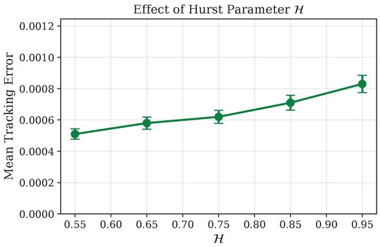
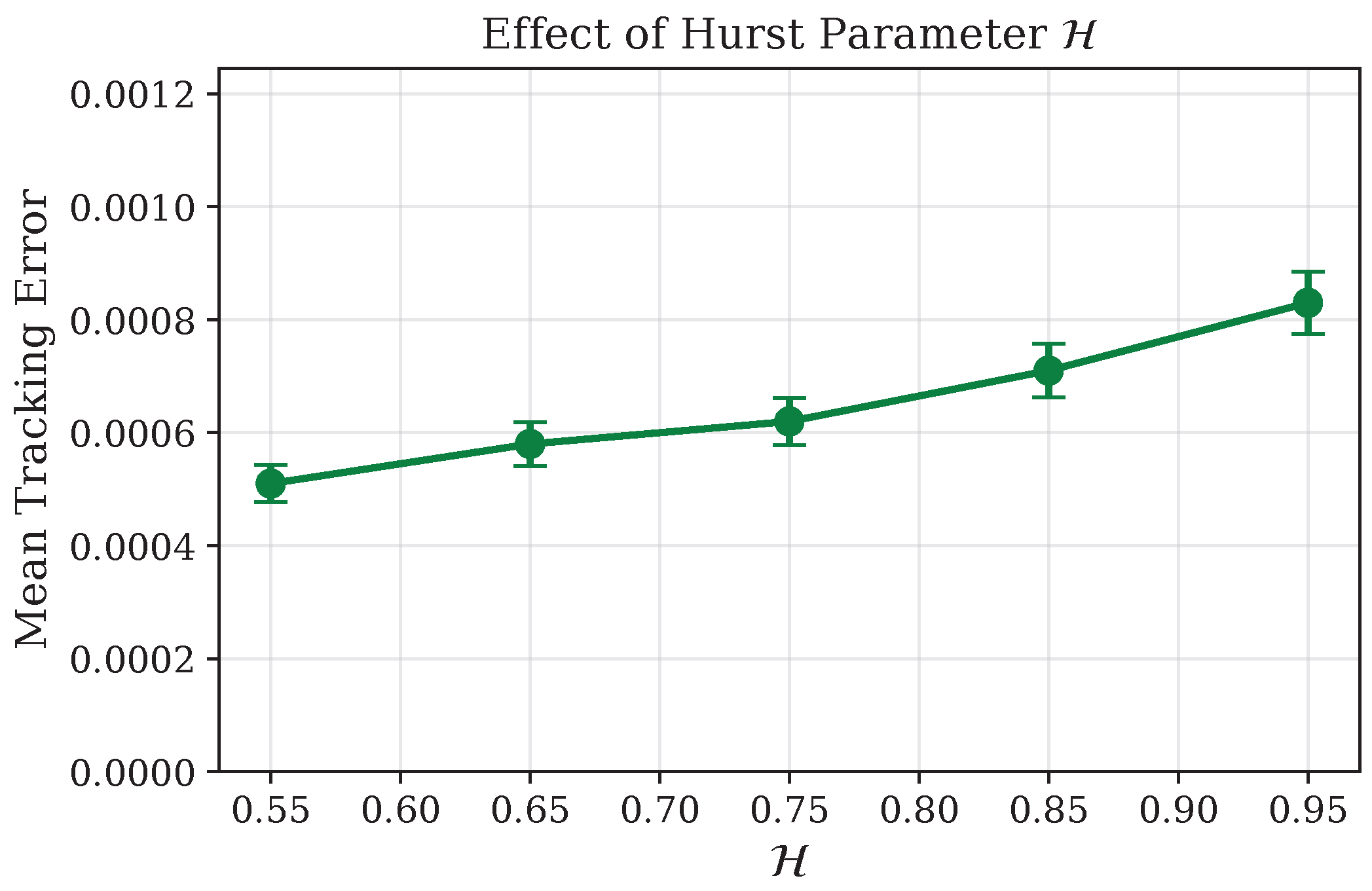
The effect of long-range dependence is studied as in Figure 4 with
Figure 4.
Time-averaged mean-square tracking error for different values of the Hurst parameter .
For the selected parameter configuration, larger values of produce a moderate increase in the empirical tracking error. This indicates that the more persistent fluctuations associated with stronger long-range dependence make trajectory tracking more difficult in the present example.
To investigate robustness with respect to stochastic perturbations, the Rosenblatt and jump coefficients are replaced by
and
where
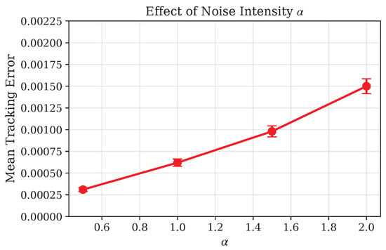
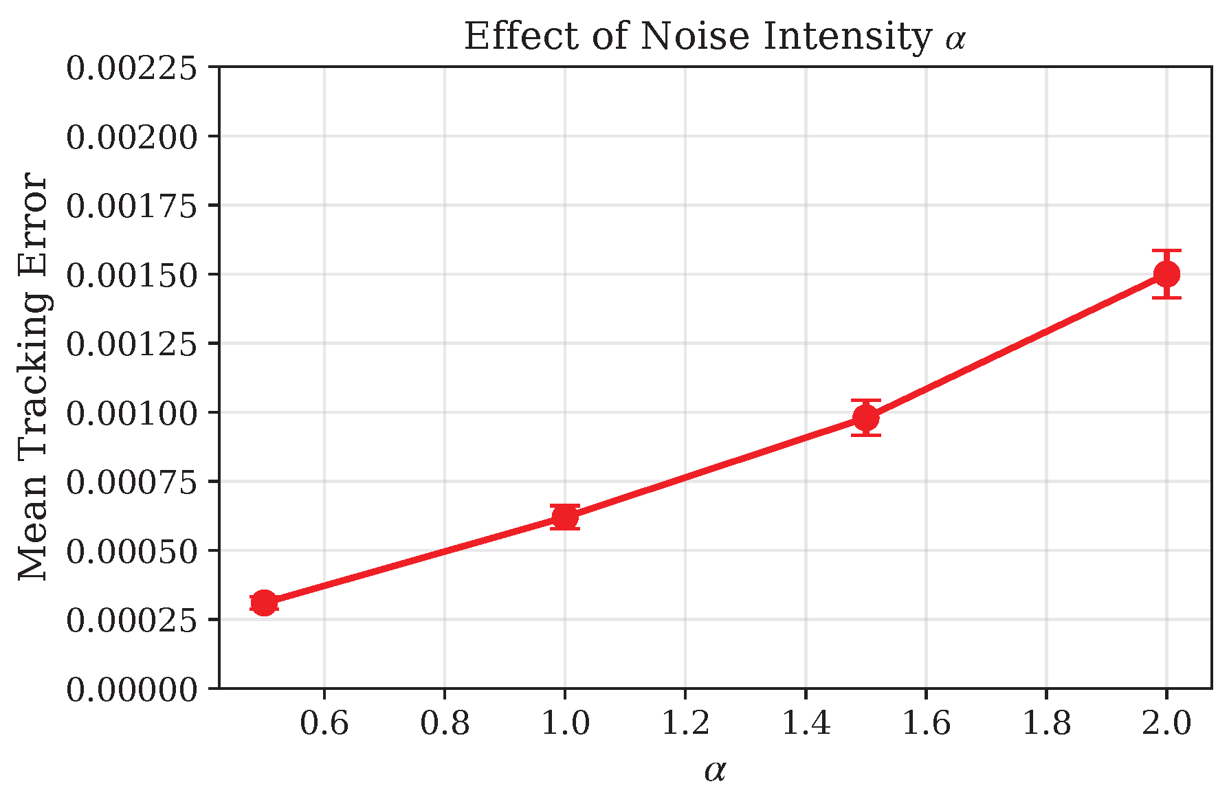
Figure 5 illustrates the influence of the noise-intensity multiplier on the overall tracking performance of the proposed control strategy. The vertical axis represents the time-averaged mean-square tracking error, while the horizontal axis corresponds to different values of the multiplier , which scales the intensity of the stochastic perturbations. Each data point represents the Monte Carlo average, and the error bars indicate the associated uncertainty over the ensemble of simulations.
Figure 5.
Time-averaged mean-square tracking error for different values of the noise-intensity multiplier .
As the value of increases from to , the time-averaged mean-square tracking error increases monotonically. For small noise intensity (), the average tracking error is approximately , indicating that the controlled trajectory follows the prescribed reference trajectory very accurately. When the noise intensity is doubled (), the error increases to approximately , while for it reaches about . The largest tracking error is observed at , where the mean error is approximately .
This behavior agrees with the theoretical expectation that stronger stochastic perturbations produce larger deviations from the desired trajectory. Nevertheless, even for the highest noise level considered, the tracking error remains below , demonstrating that the proposed trajectory realization strategy maintains satisfactory tracking accuracy under moderate stochastic disturbances. Furthermore, the relatively short error bars indicate limited variability among the Monte Carlo realizations, suggesting that the numerical performance of the controller is stable and statistically reliable.
The principal sensitivity results are summarized in Table 1. The reported standard deviations are computed from the Monte Carlo values of the time-averaged tracking error.
Table 1.
Sensitivity of the time-averaged mean-square tracking error to , , and the noise-intensity multiplier .
The sensitivity results show that the proposed open-loop control continues to reduce the tracking error throughout the investigated parameter ranges. Nevertheless, its performance deteriorates when the intensity of the stochastic perturbations becomes larger. This is consistent with the fact that the control is required to operate under a fixed admissibility constraint.
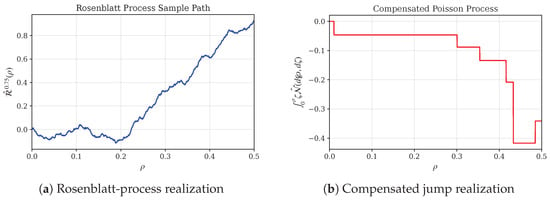
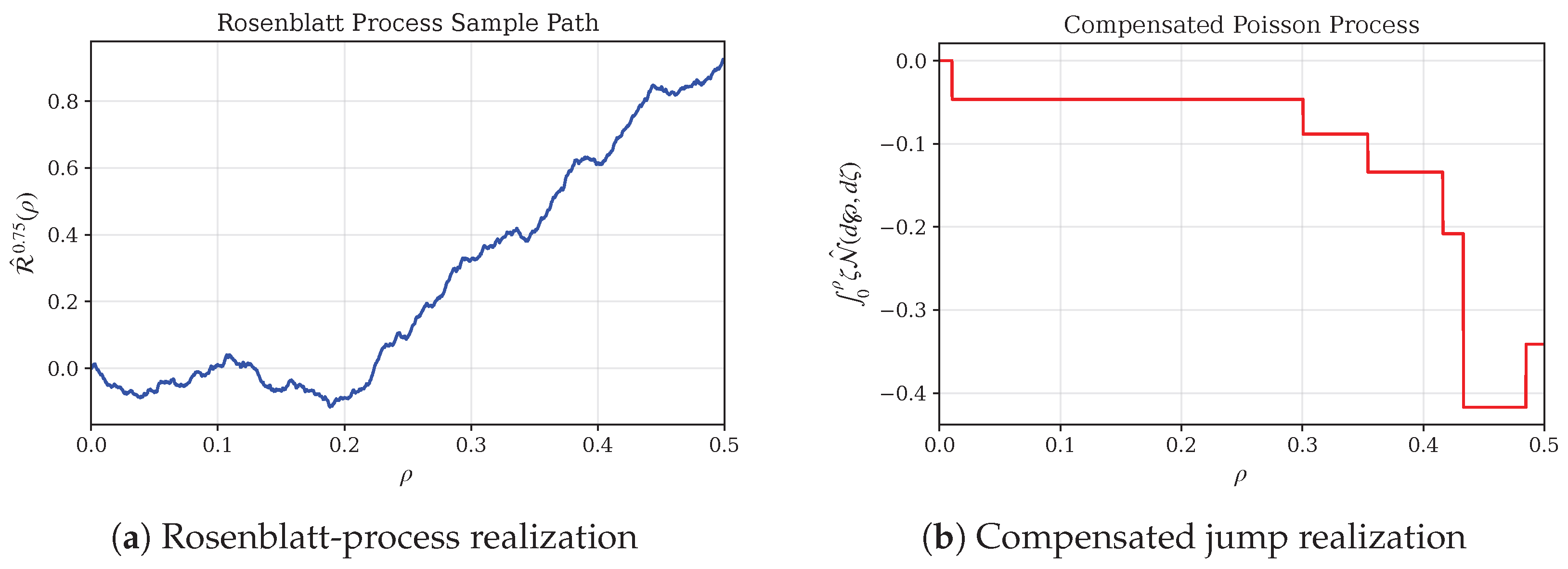
For completeness, Figure 6 displays one representative realization of each stochastic driver.
Figure 6.
Representative realizations of: (a) the Rosenblatt process ; (b) the compensated compound Poisson process.
The Rosenblatt realization exhibits persistent non-Gaussian fluctuations while the compensated Poisson process has discontinuous jumps at the jump times. These two qualitatively different sources of randomness explain the smooth and persistent variations as well as the occasional sudden changes observed in the simulated state trajectories.
The numerical experiments lead to the following observations.
First, the empirical mean of the controlled system tracks the prescribed reference trajectory significantly better than the corresponding uncontrolled trajectory. The comparison then directly shows the practical effect of the open-loop control.
Second, the pointwise mean-square tracking error is reduced after the initial transience and is small during the latter part of the simulation interval. The empirical error estimate also stabilizes when we increase the number of Monte Carlo realizations.
Thirdly, the sensitivity analysis shows that the tracking performance depends on the fractional order, the degree of long-range dependence, and the total stochastic-noise intensity. In the present example, the largest noise intensity causes the most significant decrease in the tracking accuracy.
Finally, the simulations should be understood as numerical evidence supporting the analytical results, but not as a proof of existence, uniqueness, or approximate trajectory realization. The existence and uniqueness properties are given by the theoretical arguments of the previous sections, and the present computations show the qualitative and quantitative behavior of the controlled system.
7. Conclusions
In this paper, we investigate a class of fractional stochastic delay differential systems driven jointly by the Rosenblatt process and compensated Poisson jumps in a Hilbert space setting. The main results can be summarized as follows.
First, sufficient conditions are established for the EU of mild solutions by employing KFPT and the Banach contraction principle, respectively. These results are obtained for fractional stochastic systems involving CFD, time-varying delays, Rosenblatt noise, and compensated Poisson jumps.
Next, the stability properties of the proposed system are analyzed. In particular, UHS is established in the mean-square sense, and a Mittag–Leffler-type estimate is derived to characterize the continuous dependence of mild solutions on the initial data. The analysis also clarifies the distinction between continuous dependence estimates and asymptotic decay under additional dissipativity assumptions (see Remark 2 and Corollary 1).
Furthermore, an open-loop approximate trajectory realization problem is formulated and analyzed. It is shown that any admissible reference trajectory satisfying the prescribed assumptions can be approximated arbitrarily well in the mean-square sense by a suitable feedforward control constructed through the mild solution formulation. This result concerns trajectory realization rather than classical feedback or endpoint controllability (Theorem 5).
Finally, the theoretical findings are illustrated through numerical simulations, including comparisons between controlled and uncontrolled trajectories, parameter sensitivity studies, and Monte Carlo experiments. These numerical examples demonstrate the behavior of the proposed stochastic model and support the theoretical analysis.
Future work may focus on extending the present framework to more general classes of fractional stochastic systems, such as impulsive, switching, and variable-order models, as well as systems driven by other non-Gaussian stochastic processes. Another promising direction is the study of feedback control and optimal control within the proposed analytical framework.
Author Contributions
Conceptualization, M.I.L. and N.A.; Methodology, M.I.L. and N.A.; Software, M.I.L. and N.A.; Validation, M.I.L. and N.A.; Formal analysis, M.I.L.; Investigation, M.I.L. and N.A.; Resources, M.I.L. and N.A.; Writing—original draft, M.I.L. and N.A.; Writing—review and editing, M.I.L. and N.A.; Visualization, M.I.L. and N.A.; Funding acquisition, N.A. All authors have read and agreed to the published version of the manuscript.
Funding
This work was supported by the Deanship of Scientific Research, Vice Presidency for Graduate Studies and Scientific Research, King Faisal University, Saudi Arabia [Grant No. KFU264056].
Data Availability Statement
Data is contained within the article.
Conflicts of Interest
The authors declare no conflicts of interest.
References
- Chalishajar, D.N.; Ramkumar, K.; Ravikumar, K.; Varshini, S. Trajectory controllability of Hilfer fractional neutral stochastic differential equations with deviated argument using Rosenblatt process and Poisson jumps. Differ. Equ. Dyn. Syst. 2025, 33, 453–474. [Google Scholar]
- Jalisraj, A.; Udhayakumar, R. Averaging principle for fractional stochastic differential equations driven by Rosenblatt process and Poisson jumps. J. Control Decis. 2025, 1–9. [Google Scholar] [CrossRef] [Scilit]
- Algolam, M.S.; Hussain, S.; Younis, B.A.; Osman, O.; Muflh, B.; Aldwoah, K.; Eljaneid, N. Stability and controllability analysis of stochastic fractional differential equations under integral boundary conditions driven by Rosenblatt process with impulses. Fractal Fract. 2025, 9, 146. [Google Scholar] [CrossRef] [Scilit]
- Dhayal, R.; Malik, M. Approximate controllability of fractional stochastic differential equations driven by Rosenblatt process with non-instantaneous impulses. Chaos Solitons Fractals 2021, 151, 111292. [Google Scholar] [CrossRef] [Scilit]
- Shen, G.; Sakthivel, R.; Ren, Y.; Li, M. Controllability and stability of fractional stochastic functional systems driven by Rosenblatt process. Collect. Math. 2020, 71, 63–82. [Google Scholar]
- Dhayal, R.; Malik, M. Existence and controllability of impulsive fractional stochastic differential equations driven by Rosenblatt process with Poisson jumps. J. Eng. Math. 2021, 130, 11. [Google Scholar] [CrossRef] [Scilit]
- Padder, A.; Almutairi, L.; Qureshi, S.; Soomro, A.; Afroz, A.; Hincal, E.; Tassaddiq, A. Dynamical analysis of generalized tumor model with Caputo fractional-order derivative. Fractal Fract. 2023, 7, 258. [Google Scholar] [CrossRef] [Scilit]
- Aly, E.S.; Liaqat, M.I.; Alshammari, S.; El-Morshedy, M. Well-posedness and stability of fractional stochastic integro-differential equations with general memory effects. AIMS Math. 2025, 10, 22265–22293. [Google Scholar] [CrossRef] [Scilit]
- Djaouti, A.M.; Liaqat, M.I. Generalized Grönwall inequality and Ulam–Hyers stability in Lp space for fractional stochastic delay integro-differential equations. Mathematics 2025, 13, 1252. [Google Scholar] [CrossRef] [Scilit]
- Tudor, C.A. Analysis of Variations for Self-Similar Processes: A Stochastic Calculus Approach; Springer: Cham, Switzerland, 2013. [Google Scholar]
- Maejima, M.; Tudor, C.A. Wiener integrals and Rosenblatt process. Stoch. Anal. Appl. 2012, 30, 688–704. [Google Scholar]
- Arras, B. A white noise approach to the Rosenblatt process. Stoch. Process. Their Appl. 2019, 129, 4565–4594. [Google Scholar]

Disclaimer/Publisher’s Note: The statements, opinions and data contained in all publications are solely those of the individual author(s) and contributor(s) and not of MDPI and/or the editor(s). MDPI and/or the editor(s) disclaim responsibility for any injury to people or property resulting from any ideas, methods, instructions or products referred to in the content. |
© 2026 by the authors. Licensee MDPI, Basel, Switzerland. This article is an open access article distributed under the terms and conditions of the Creative Commons Attribution (CC BY) license.