Memory-Dependent Dynamics of Trachoma with Real Data Analysis from Cameroon via Fractional Framework

Abstract

This study models trachoma transmission in Cameroon using a deterministic approach with integer and fractional-order derivatives, incorporating direct, fly-mediated, and environmental transmission routes. Fitting disease data from 1990–2019, the model forecasts trachoma prevalence until 2035. The research confirms the solution existence and uniqueness, calculates the basic reproduction number ${\mathcal{R}}_0^{\lambda }$ where $\lambda \in (0,1]$ represents the fractional-order parameter, and analyzes equilibrium stability. A stable trachoma-free equilibrium exists when ${\mathcal{R}}_0^{\lambda }<1$, while an endemic equilibrium is proven stable for ${\mathcal{R}}_0^{\lambda }>1$ under specific conditions. Calibration of a fractional model with Cameroon data yielded an ${\mathcal{R}}_0$ of 1.169 (indicating endemicity) and identified an optimal fractional order of $\lambda =0.98$. By calculating the strength number, we found that another epidemic wave could occur in 50 years. Global sensitivity analysis highlighted key parameters affecting trachoma dynamics. A numerical scheme of the model based on the Adams–Bashforth–Moulton method is constructed and its stability demonstrated. It is then used to perform several numerical simulations, first to validate the theoretical results obtained, and then to compare the different models (statistical and deterministic). The conclusion is reached that the disease will persist in the population (${\mathcal{R}}_0>1$), although the statistical model shows that it could disappear by 2030. This proves that, for trachoma dynamics in Cameroon, it is advisable to use a deterministic model.

1. Introduction

Trachoma is an infectious disease that is spread by flies and contact with an infected person’s eyes or nose. It is regarded as a neglected tropical disease. An obligatory intracellular bacterium known as Chlamydia Trachomatis is the primary cause of infected blindness globally [1,2]. Currently, the World Health Organization (WHO) prioritizes the surveillance and eradication of 17 neglected tropical diseases (NTDs) through improved therapeutic and preventive methods or preventive treatments. Trachoma is one of these diseases [1,3]. Cameroon is one of 42 countries where this infectious illness is a public health concern. Approximately 1.9 million individuals are blind or visually impaired as a result of it [4]. According to data from June 2022, around 125 million individuals are at risk of blindness and reside in areas where trachoma is common [4]. In Cameroon, trachoma remains a public health problem in several health districts in the north and the far north of the country. Studies have shown that trachoma is present in 17 health districts in two regions (North and Far North) [5,6]. Poor housing and hygiene contribute to Chlamydia trachomatis spread, which can be transmitted through direct personal contact, contaminated garments, flies, and infected objects, as well as through eye or nose secretions [7].

Since Sir Ross’s groundbreaking research on malaria [8], several works have been conducted to understand the transmission dynamics of infectious diseases (see for example [9,10,11] and the references therein). The recent contributions of epidemic models to understanding the complex dynamics of diseases are of great importance [12,13], enabling researchers to assess the impact of various control strategies [14], and analyze the transmission dynamics of infectious diseases [15]. Regarding trachoma, several hypotheses have been proposed to explain its transmission dynamics and control programs [16,17]. Efficient control methods for trachoma have been introduced using these mathematical models [18,19,20]. Furthermore, a mathematical model was devised by Salisu Muhammad et al. in [3] to investigate the dynamics of blinding trachoma transmission in Nigeria. They considered the dynamics of human-vector transfer as well as person-to-person transmission. In [21], Ndisabiye et al. used an ordinary differential equation that incorporates an environmental transmission component.

There is a need to develop a comprehensive model that incorporates key factors that have been overlooked in existing frameworks. Using the fractional-order derivative of Caputo, the current study suggested a new Susceptible human–Exposed human–Infectious human–Recovered human–Susceptible fly–Exposed fly–Infectious fly–Bacteria (SEIR-SEI-B) compartmental model of trachoma that considers transmission between humans, the environment, and between humans and flies. Real dynamic systems are better described using non-integer order dynamic models, unlike traditional calculus which relies on differentiation and integration at integer order. The way that people see, depict, and interact with the natural world can be drastically changed by fractional calculus. In recent years, there has been a discernible rise in the use of different fractional operators to represent the provided problems. This approach has gained widespread acceptance as a conventional technique for researching the transmission of illnesses [22,23]. The suggested trachoma model is formulated using the Caputo fractional order derivative, which enables more thorough model dynamics observation using real-time data [24]. Compared to alternative fractional definitions (like Riemann–Liouville), the Caputo fractional derivative is preferred for modeling real-world issues because it enables the inclusion of initial and boundary conditions in a manner consistent with classical, integer-order differential equations. Because of this, they are simple to understand and resolve in scientific and engineering settings.

This study aims to develop and analyze a deterministic model using integer and fractional derivatives of the Caputo type to understand the transmission dynamics of trachoma in Cameroon. The model considers vector transmission, direct transmission, and environmental transmission. The areas of application of fractional calculus are diverse. Indeed, it has been proven that fractional operator models are better suited to modeling certain phenomena such as groundwater pollution [25,26], as well as the transmission of infectious diseases [27,28]. The most used fractional operators in infectious disease modeling are the Caputo operator [29,30], the Caputo–Fabrizio operator [31], and the Atangana–Baleanu operator [32,33]. Among these three fractional operators, the one which is closest to the classical or integer derivatives is the Caputo operator whose derivative of a constant is zero (exactly as in the case of the integer derivative). In the present work we will use the derivatives in the sense of Caputo. The specific objectives are listed as follows:

(i)

Choose the statistical model which better fits the reported cases of trachoma in Cameroon and project the evolution of the disease in the short and medium term;

(ii)

Create a new deterministic model considering direct, vectorial, and environmental transmission, utilizing a fractional operator in the Caputo sense;

(iii)

Calibrate the deterministic model by estimating parameters using data from Cameroon;

(iv)

Find the fractional-order parameter’s ideal value that best fits the reported cases;

(v)

Make a short- and medium-term projection of trachoma in Cameroon using the deterministic model;

(vi)

Compare the statistical model and the deterministic model.

This is how the current document is structured: In Section 2, we present the reported data on trachoma in Cameroon and make some predictions using a statistical function. Section 3 is devoted to preliminary definitions on the Riemann–Liouville integral and the Caputo fractional-order derivative. We formulate our deterministic model, as well as its theoretical analysis in Section 4. Section 5 is reserved for model calibration and forecasting. The numerical scheme, as well as its stability, that will be used for numerical simulations will be constructed in Section 6. This section also encompasses numerical simulations and discussions. The work is finished with a conclusion.

2. Real Data and Statistical Model

We provide here the notified cases of trachoma in Cameroon for the period from 1990 to 2019 [34], and consequently do future forecasts of trachoma in Cameroon for the period from 2020 to 2035, using the MatLab 2016 software package cftool. The Gaussian function of order 5 is the function that most closely matches the Cameroon data. The expression of this function is given as follows:

$$\begin{array}{c}\hfill f_{\mathrm{Cameroon}}\left(x\right)=\sum _{i=1}^5{a}_{i}exp\left\{-{\left({\displaystyle \frac{x-b_i}{c_i}}\right)}^2\right\},\end{array}$$

(1)

where $a_1=1561$, $b_1=2019$, $c_1=3.528$, $a_2=3194$, $b_2=1998$, $c_2=3.883$, $a_3=9936$, $b_3=1992$, $c_3=10.64$, $a_4=2778$, $b_4=2001$, $c_4=2,371$, $a_5=4100$, $b_5=2010$, and $c_5=8.948$.

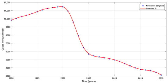
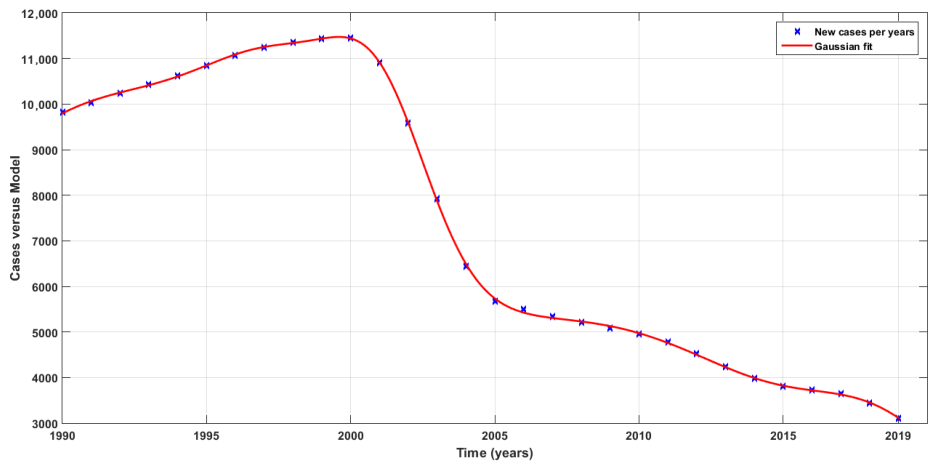
The result is shown in Figure 1.

Figure 1. Fifth-order Gaussian fit (red line) using trachoma cases notified in Cameroon between 1990 and 2019 (blue stars).

Table 1 lists the attributes of this fit-type function.

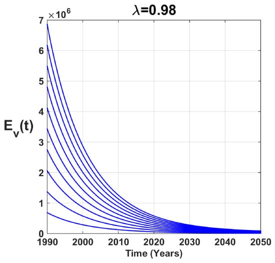
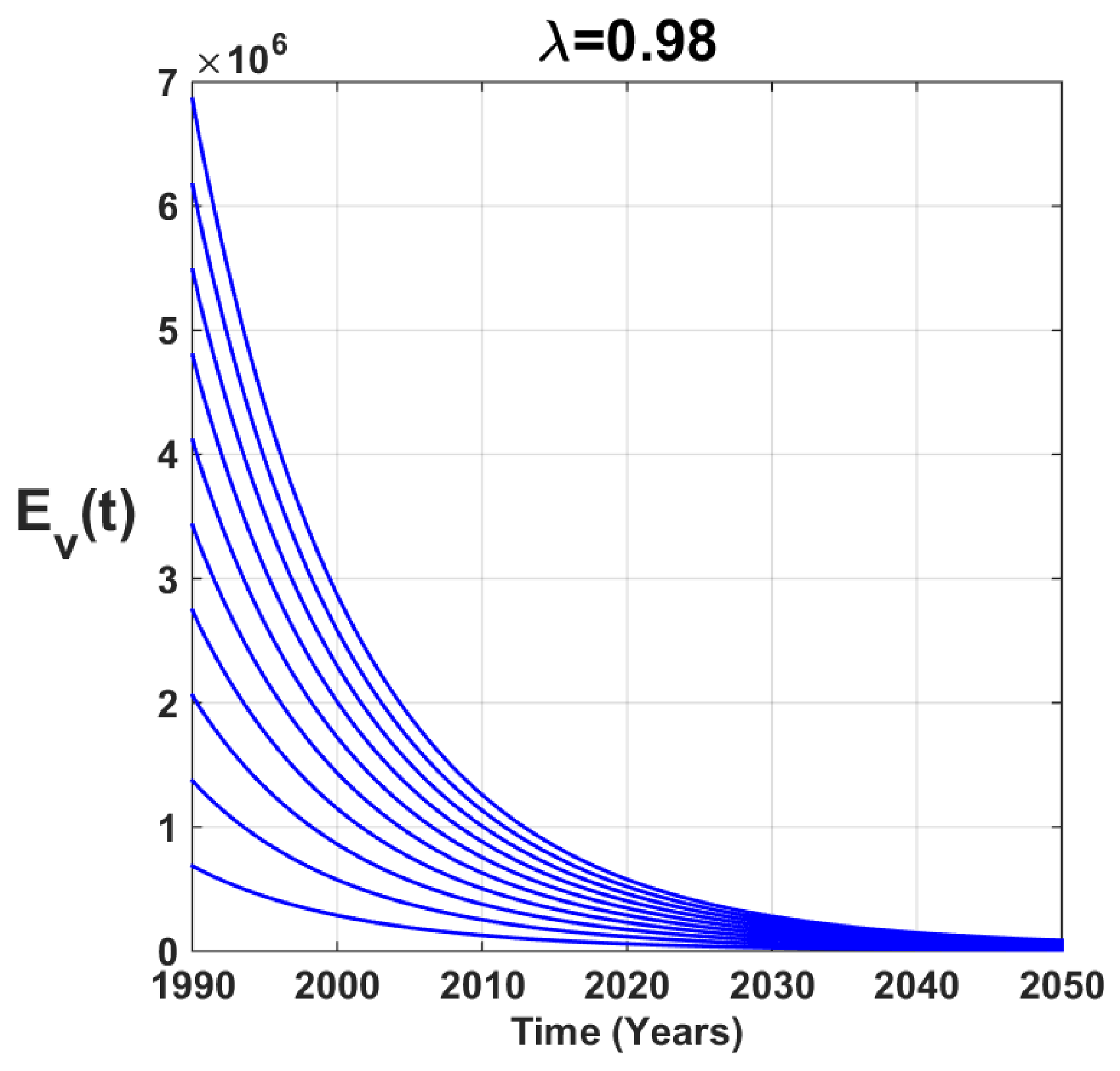
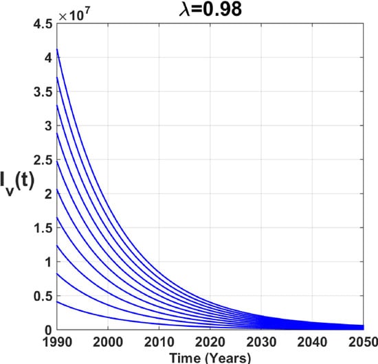
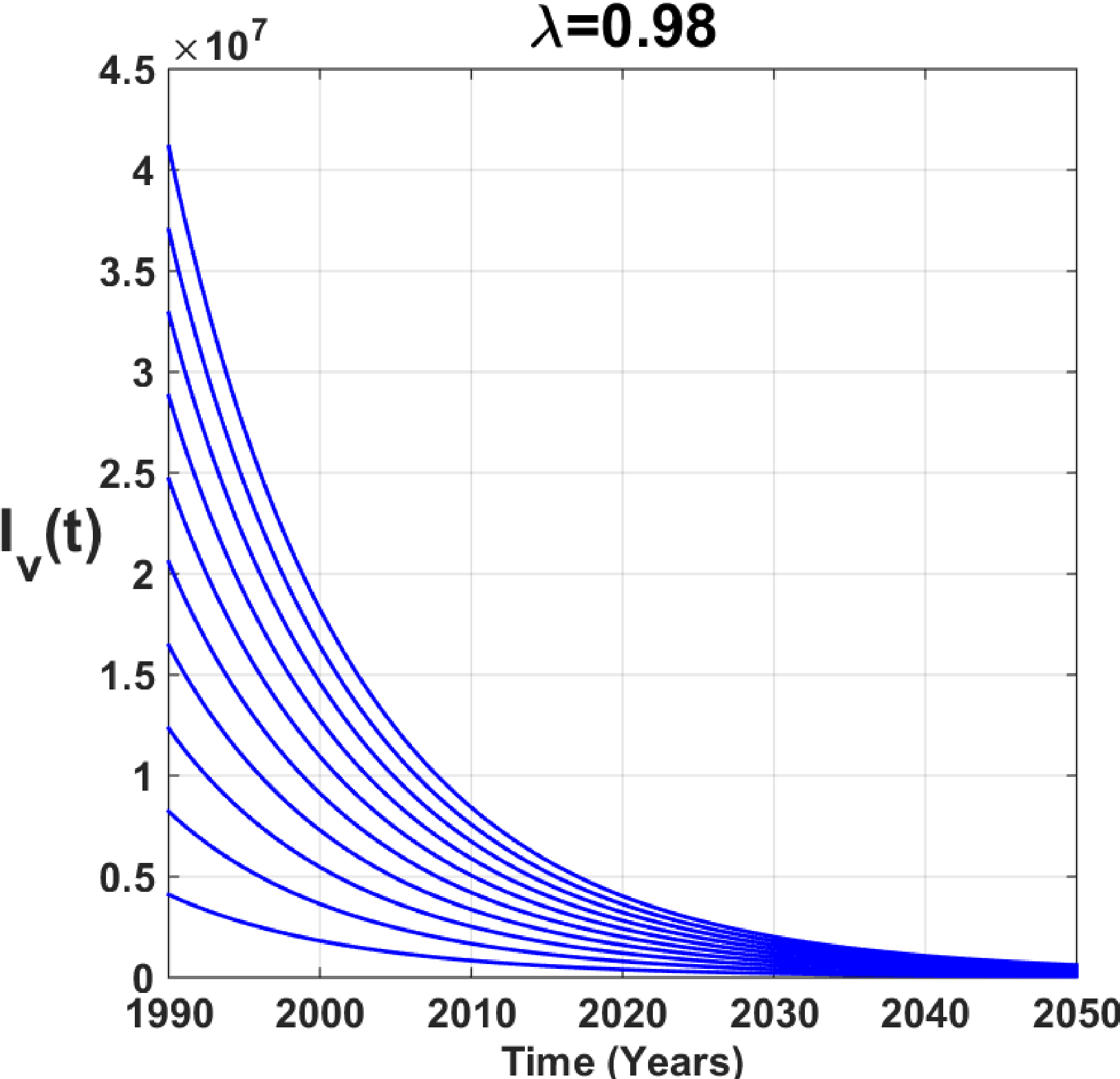
Table 1. Statistical results of model fitting and 5th-order Gaussian function. y stands for trachoma cases, and t stands for year.

Data	Fit Type	SSE	R-Square	DFE	Adj R-sq	RMSE	Coeff
y vs. t	gauss5	2.2409 $\times {10}^4$	0.9999	15	0.9998	38.6514	15

In Cameroon, new cases of trachoma numbered around 9900 in the 1990. Between 1990 and 2000, the number of new cases of trachoma rose steadily to around 11,500. This growth can be explained by the fact that there was no effective control strategy for this disease. Then, between 2000 and 2005, there was a decline in the curve (11,500 to 5700 new cases), which can be explained by several factors: awareness of the dangers of the disease and the need to prevent and treat it. In Cameroon, trachoma control strategies from 2000 to 2005 focused on the distribution of antibiotics (Azithromycin), surgical interventions for advanced cases of trachoma, awareness raising to prevent the spread of the disease and application of the SAFE strategy. These interventions were supported by international partners such as the World Health Organization (WHO), the United Nations Children’s Fund (UNICEF), the Program to Fight Blindness in Africa (AFRO), and the United Nations Population Fund (UNFPA) [35]. Finally, from 2005 to 2019, the number of new cases will continue to fall steadily, to around 3000. This can be explained by the fact that the strategies applied have considerably reduced the prevalence of trachoma in Cameroon.

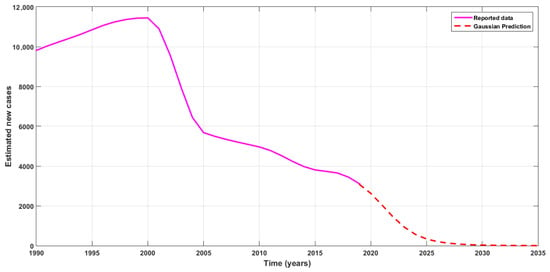
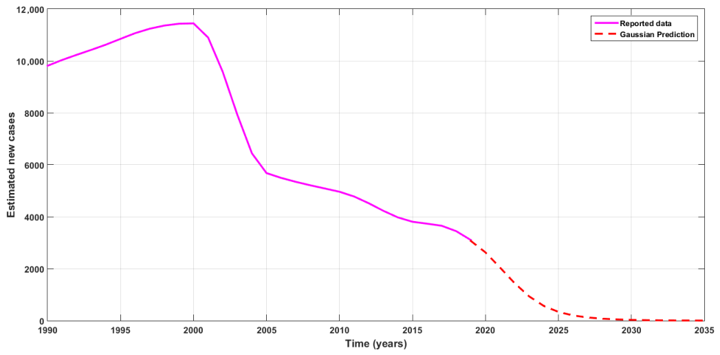
We now use the above function to predict new cases of trachoma in Cameroon over the next sixteen years (from 2020 to 2035). The result is shown in Figure 2.

Figure 2. Cases of trachoma notified in Cameroon between 1990 and 2019 (purple line) and forecasts for the next sixteen (16) years (broken line).

According to Figure 2, it appears that by intensifying measures to combat trachoma in Cameroon, we can predict that trachoma will tend to disappear by 2035. However, we will see that by considering a deterministic model (with Caputo’s fractional order derivative), this conclusion could be erroneous, as the disease will persist in the population.

3. Preliminary Definitions and Result

Definition 1

(The Riemann–Liouville (R-L) integral [36]). Let h $\in C\left(\right[a,b\left]\right)$. The R-L integral of order $\iota >0$ of h is defined as follows:

$${\mathcal{J}}_a^{\iota }h\left(x\right)={\displaystyle \frac{1}{\Gamma \left(\iota \right)}}{\int }_a^x{(x-s)}^{\alpha -1}h\left(\eta \right)ds.\iota \notin \mathbb{N}$$

(2)

Definition 2

(Caputo derivative [36]). Let $h\in {\mathcal{C}}^l\left([0;d]\right)$, $d>0$, $\iota \in \mathbb{R}$, $l\in \mathbb{N}$ such that $\iota \in (-1+l,l)$. The Caputo fractional-order derivative of order ι of h is given by the following:

$${}_0{}^C\mathcal{D}_t^{\iota }\left(h\left(\eta \right)\right)={\displaystyle \frac{1}{\Gamma (l-\iota )}}{\int }_0^s{\left(s-\varpi \right)}^{l-\iota -1}{h}^{\left(l\right)}\left(\varpi \right)d\varpi ,s>0.$$

(3)

If fractional order $\iota =1$, then ${}_0{}^C\mathcal{D}_t^{\iota }(•)={\displaystyle \frac{d}{dt}}(•)$.

Theorem 1

(Barrier Theorem [37]). Let $\dot{\mathcal{X}}=h\left(\mathcal{X}\right)$, with $h:{\rm Y}\subset {\mathbb{R}}^n\to {\mathbb{R}}^n$ a ${\mathcal{C}}^1$ function. Let $G:{\mathbb{R}}^n\to \mathbb{R}$ be a ${\mathcal{C}}^1$ function, $\Xi =\left\{\mathcal{X}\in {\mathbb{R}}^n:F\left(\mathcal{X}\right)\le 0\right\}$ a closed set with $\partial \Xi =\left\{X\in {\mathbb{R}}^n:F\left(\mathcal{X}\right)=0\right\}$ its boundary. If $\forall \mathcal{X}\in \partial \Xi$, $\nabla F\left(\mathcal{X}\right)\ne 0$ and $⟨h\left(X\right)|\nabla F(\mathcal{X})⟩\le 0$, then Ξ is positively invariant.

4. Formulation of the Trachoma Deterministic Model and Its Analysis

4.1. Formulation of the Trachoma Deterministic Model

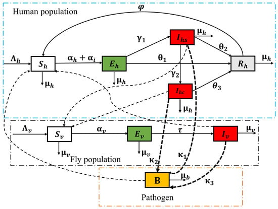
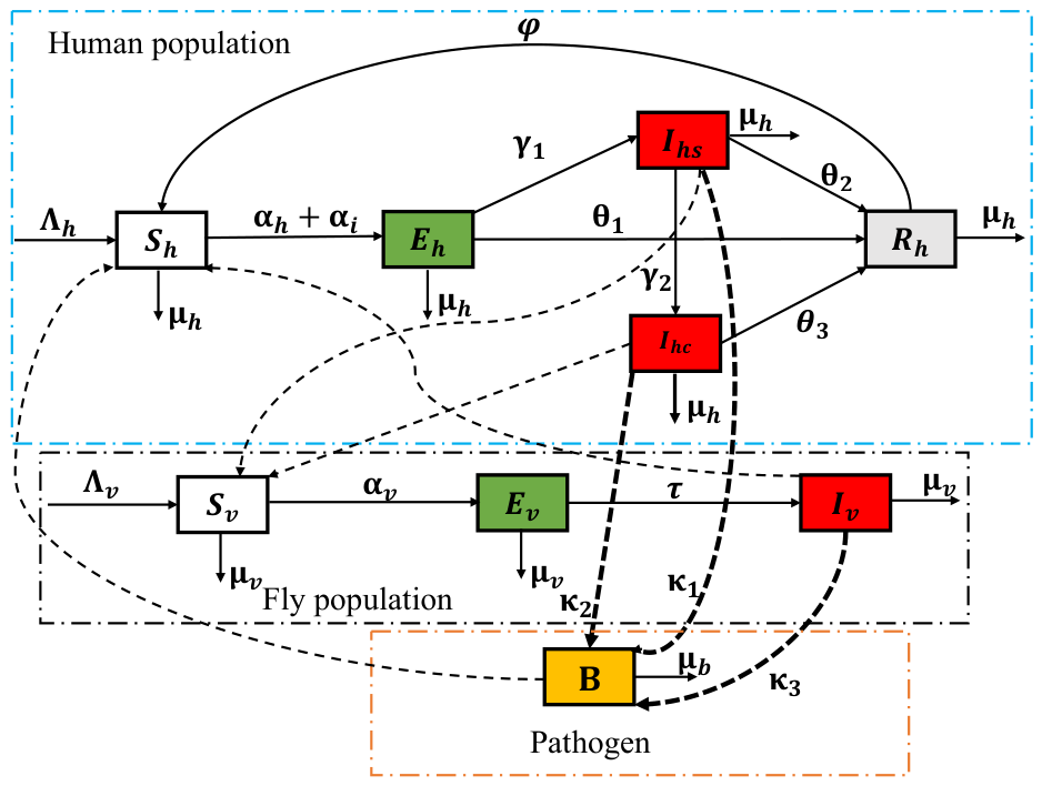
Three subpopulations are taken into consideration: the human population, the fly population, and the population of environmental free pathogens. The human population is divided into five compartments: susceptible, infected, infectious, trachomatous trichiasis/corneal opacity, and temporarily recovered. The steady recruitment rate ${\Lambda }_h$ increases the number of susceptible individuals, but direct contact with an infectious fly $I_v$ or contaminated tools causes them to drop at rates ${\alpha }_h$ and ${\alpha }_i$, respectively, or they die naturally at a rate ${\mu }_h$. Those that are vulnerable get infected but not yet contagious (latency stage) after coming into touch with an infected person, fly, or instrument. Rates ${\theta }_1$ and ${\gamma }_1$ of $E_h$ will be restored, while rates ${\theta }_2$ will be restored, resulting in the change of $I_{hs}$ and $I_{hc}$. A rate ${\theta }_3$ of $I_{hc}$ will become recovered $R_h$ following treatment. Human life span is $1/{\mu }_h$, since humans die at a natural rate ${\mu }_h$. A steady recruitment rate of ${\Lambda }_v$ increases susceptible flies, but contact with an infectious human ($I_{hs}$ or $I_{hc}$) causes them to decline at a rate of ${\alpha }_v$ or a natural death at a rate of ${\mu }_v$. After $1/\tau$ days, infected flies become contagious. Throughout their lives, infected flies continue to spread disease, the cause of the fly subpopulation’s lack of a recovered compartment. The infectious flies, which act as agents of environmental contamination, infectious humans, $I_{hs}$, and $I_{hc}$ all contribute to the growth of the pathogen population, represented by B. $N_h=E_h+S_h+I_{hs}+R_h+I_{hc}$ represents the total host population at any given moment t, whereas $N_v=I_v+E_v+S_v$ represents the total size of the fly population. The definitions of ${\alpha }_h$, ${\alpha }_i$, and ${\alpha }_v$ which represent the force of infection (FOI), are given by

$${\alpha }_h^{\lambda }=a_h^{\lambda }{b}_v^{\lambda }{\displaystyle \frac{I_v}{I_v{\psi }_1+1}},{\alpha }_i^{\lambda }={\nu }^{\lambda }{\displaystyle \frac{B}{K+B}},{\alpha }_v=a_v^{\lambda }{b}_v^{\lambda }{\displaystyle \frac{I_{hs}+I_{hc}}{\left(I_{hc}+I_{hs}\right){\psi }_2+1}}.$$

(4)

where $b_v$ denotes the number of infectious contacts an infectious fly makes each day, $a_h$ and $a_v$ show the likelihood that an infectious fly will spread a pathogen to a susceptible human and a susceptible human, respectively, $\nu$ denotes the rate of exposure to environmental pathogens, K is the half-saturation rate, and ${\psi }_1$ and ${\psi }_2$ represent the saturated parameters.

Figure 3 displays a graphic of the suggested model that explains how trachoma spreads.

Figure 3. The mathematical model of trachoma transmission represented in compartments. Arrows show which way an infection spreads from one person to another. ${\alpha }_h^{\lambda }=a_h^{\lambda }{b}_v^{\lambda }{\displaystyle \frac{I_v}{I_v{\psi }_1+1}}$, ${\alpha }_i^{\lambda }={\nu }^{\lambda }{\displaystyle \frac{B}{K+B}}$, and ${\alpha }_v=a_v^{\lambda }{b}_v^{\lambda }{\displaystyle \frac{I_{hs}+I_{hc}}{\left(I_{hc}+I_{hs}\right){\psi }_2+1}}$.

Table 2 provides a comprehensive overview of the variables and parameters of the fractional model.

Table 2. An explanation of the model symbols and variables.

Variables	Description
$S_h\left(t\right)$,$S_v\left(t\right)$	Susceptible humans and flies
$E_h\left(t\right)$	Humans and flies with latent infection
$I_{hs}\left(t\right)$	People who have trachoma in the early stages of infection
$I_{hc}\left(t\right)$	People who have trachoma infections during the TT and CO stages
$R_h\left(t\right)$	Cured humans
$I_v\left(t\right)$	Contagious flies
B	Environmental free pathogens
Symbols	Description
${\Lambda }_v$, ${\Lambda }_h$	Constant rates of fly and human recruitment
${\mu }_v$, ${\mu }_h$,	Fly and human natural mortality rates
${\mu }_b$	The pathogen’s natural death rate
${\gamma }_1$	Rate of transition between $E_h$ and $I_{hs}$
${\gamma }_2$	Rate of transition between $I_{hs}$ and $I_{hc}$
$\phi$	Rate of immunity decline
$1/\tau$	Latency time in flies
${\theta }_1$	Latent individuals’ pace of recovery
${\theta }_2$	Recovery rate of $I_{hs}$
${\theta }_3$	Recovery rate of $I_{hc}$
${\kappa }_1$	$I_{hs}$’s contribution to the spread of microorganisms in the environment
${\kappa }_2$	$I_{hc}$’s contribution to the spread of microorganisms in the environment
${\kappa }_3$	$I_v$’s role in the environment’s bacterial proliferation
$a_v$	Rate of transmission between $S_v$ and $E_v$
$\nu$	Rate of environmental pathogen exposure
$a_h$	Transmission rate ($S_h$ has contacted $I_h$) from $S_h$ to $E_h$
$b_v$	Infected fly contact rate
K	Rate of half-saturation
${\psi }_1$, ${\psi }_2$	Parameters of saturation

Figure 3 provides the following system:

$$\left\{\begin{array}{cc}{}_0{}^C\mathcal{D}_t^{\lambda }{S}_h\hfill & ={\Lambda }_h^{\lambda }-{\alpha }_h^{\lambda }{S}_h-{\alpha }_i^{\lambda }{S}_h+{\phi }^{\lambda }{R}_h-{\mu }_h^{\lambda }{S}_h,\hfill \\ {}_0{}^C\mathcal{D}_t^{\lambda }{E}_h\hfill & ={\alpha }_h^{\lambda }{S}_h+{\alpha }_i^{\lambda }{S}_h-{\gamma }_1^{\lambda }{E}_h-{\mu }_h^{\lambda }{E}_h-{\theta }_1^{\lambda }{E}_h,\hfill \\ {}_0{}^C\mathcal{D}_t^{\lambda }{I}_{hs}\hfill & ={\gamma }_1^{\lambda }{E}_h-{\gamma }_2^{\lambda }{I}_{hs}-{\mu }_h^{\lambda }{I}_{hs}-{\theta }_2^{\lambda }{I}_{hs}\hfill \\ {}_0{}^C\mathcal{D}_t^{\lambda }{I}_{hc}\hfill & ={\gamma }_2^{\lambda }{I}_{hs}-{\theta }_3^{\lambda }{I}_{hc}-{\mu }_h^{\lambda }{I}_{hc},\hfill \\ {}_0{}^C\mathcal{D}_t^{\lambda }{R}_h\hfill & ={\theta }_1^{\lambda }{E}_h+{\theta }_2^{\lambda }{I}_{hs}+{\theta }_3^{\lambda }{I}_{hc}-{\phi }^{\lambda }{R}_h-{\mu }_h^{\lambda }{R}_h,\hfill \\ {}_0{}^C\mathcal{D}_t^{\lambda }{S}_v\hfill & ={\Lambda }_v^{\lambda }-{\alpha }_v^{\lambda }{S}_v-{\mu }_v^{\lambda }{S}_v,\hfill \\ {}_0{}^C\mathcal{D}_t^{\lambda }{E}_v\hfill & ={\alpha }_v^{\lambda }{S}_v-{\tau }^{\lambda }{E}_v-{\mu }_v^{\lambda }{E}_v,\hfill \\ {}_0{}^C\mathcal{D}_t^{\lambda }{I}_v\hfill & ={\tau }^{\lambda }{E}_v-{\mu }_v^{\lambda }{I}_v,\hfill \\ {}_0{}^C\mathcal{D}_t^{\lambda }B\hfill & ={\kappa }_1^{\lambda }{I}_{hs}+{\kappa }_2^{\lambda }{I}_{hc}+{\kappa }_3^{\lambda }{I}_v-{\mu }_b^{\lambda }B,\hfill \end{array}\right.$$

(5)

where ${}_0{}^C\mathcal{D}_t^{\lambda }$ denotes the Caputo fractional derivative operator of order $\lambda$. Note that if $\lambda =1$ then system (5) is equivalent to the model with classical derivative ${\displaystyle \frac{d}{dt}}(•)$. To preserve the physical units, the fractional order parameter $\lambda$ is placed in the power of certain parameters of the model.

4.2. Mathematical Analysis

Here, we demonstrate the existence, uniqueness, positivity, and boundedness of the fractional model’s solutions.

Let $\mathcal{X}:=\left(S_h,E_h,I_{hs},I_{hc},R_h,S_v,E_v,I_v,B\right)$, $\mathcal{Q}={(F_1,F_2,\dots ,9)}^t$ where

$$\left\{\begin{array}{cc}{F}_1\hfill & ={\Lambda }_h^{\lambda }-{\alpha }_h^{\lambda }{S}_h-{\alpha }_i^{\lambda }{S}_h+{\phi }^{\lambda }{R}_h-{\mu }_h^{\lambda }{S}_h,\hfill \\ F_2\hfill & ={\alpha }_h^{\lambda }{S}_h+{\alpha }_i^{\lambda }{S}_h-{\gamma }_1^{\lambda }{E}_h-{\mu }_h^{\lambda }{E}_h-{\theta }_1^{\lambda }{E}_h,\hfill \\ F_3\hfill & ={\gamma }_1^{\lambda }{E}_h-{\gamma }_2^{\lambda }{I}_{hs}-{\mu }_h^{\lambda }{I}_{hs}-{\theta }_2^{\lambda }{I}_{hs}\hfill \\ F_4\hfill & ={\gamma }_2^{\lambda }{I}_{hs}-{\theta }_3^{\lambda }{I}_{hc}-{\mu }_h^{\lambda }{I}_{hc},\hfill \\ F_5\hfill & ={\theta }_1^{\lambda }{E}_h+{\theta }_2^{\lambda }{I}_{hs}+{\theta }_3^{\lambda }{I}_{hc}-{\phi }^{\lambda }{R}_h-{\mu }_h^{\lambda }{R}_h,\hfill \\ F_6\hfill & ={\Lambda }_v^{\lambda }-{\alpha }_v^{\lambda }{S}_v-{\mu }_v^{\lambda }{S}_v,\hfill \\ F_7\hfill & =-E_v{\mu }_v^{\lambda }+{\alpha }_v^{\lambda }{S}_v-{\tau }^{\lambda }{E}_v,\hfill \\ F_8\hfill & =-I_v{\mu }_v^{\lambda }+{\tau }^{\lambda }{E}_v,\hfill \\ F_9\hfill & =I_{hs}{\kappa }_1^{\lambda }+I_{hc}{\kappa }_2^{\lambda }+I_v{\kappa }_3^{\lambda }-B{\mu }_b^{\lambda }.\hfill \end{array}\right.$$

(6)

The compact form of the dynamic system (5) is as follows:

$$\left\{\begin{array}{c}{D}_t^{\lambda }\mathcal{X}\left(t\right)=\mathcal{Q}(t,\mathcal{X}\left(t\right)),\hfill \\ E_0=\mathcal{X}\left(0\right)\ge 0,\hfill \\ 0\le t\le t_f,\hfill \\ 0<\lambda \le 1.\hfill \end{array}\right.$$

(7)

The integral form of Equation (7) is given by the following:

$$\mathcal{X}\left(t\right)=E_0+{\left(\Gamma \left(\lambda \right)\right)}^{-1}{\int }_0^t\mathcal{Q}(\eta ,\mathcal{X}\left(\eta \right)){(-\eta +t)}^{-1+\lambda }d\eta .$$

(8)

Let $\mathcal{T}=\mathcal{C}([0,t_f];\mathbb{R})$. $\mathcal{T}$ is endowed with the norm

$${\left|\right|\mathcal{X}\left|\right|}_{\omega }=\underset{t\in [0,t_f]}{sup}\left\{\right|\mathcal{X}\left(t\right)\left|\right\},$$

(9)

where $\left|\mathcal{X}\left(t\right)\right|={\displaystyle \sum _{i=1}^9}\left|{\mathcal{X}}_i\left(t\right)\right|$. Note that ${\mathcal{X}}_i\left(t\right)\in \mathcal{T}$, $i=1,2,...,9$. In addition, we define $\mathcal{H}:\mathcal{T}\to \mathcal{T}$ by

$$\left(\mathcal{H}\mathcal{X}\right)\left(t\right)=E_0+{\left(\Gamma \left(\lambda \right)\right)}^{-1}{\int }_0^t{(-\eta +t)}^{\lambda -1}\mathcal{Q}(\eta ,\mathcal{X}\left(\eta \right))d\eta ,$$

(10)

which is well defined because $\mathcal{Q}$ is continuous.

We first prove the positivity of the model solution and its boundedness.

Theorem 2

(Positivity). For all $t>0$, a solution $\mathcal{X}$ of (5) with $E_0\in {\mathbb{R}}_{+}^9$, is non-negative.

Proof. 

We have, from (5),

$$\left\{\begin{array}{cc}{\left.{}_0{}^C\mathcal{D}_t^{\lambda }{S}_h\right|}_{{\mathcal{X}}_1=0,{\mathcal{X}}_5\ge 0}\hfill & ={\Lambda }_h^{\lambda }+{\phi }^{\lambda }{R}_h>0,\hfill \\ {\left.{}_0{}^C\mathcal{D}_t^{\lambda }{E}_h\right|}_{{\mathcal{X}}_2=0,{\mathcal{X}}_i\ge 0,i\ne 2}\hfill & ={\alpha }_h^{\lambda }{S}_h+{\alpha }_i^{\lambda }{S}_h\ge 0,\hfill \\ {\left.{}_0{}^C\mathcal{D}_t^{\lambda }{I}_{hs}\right|}_{{\mathcal{X}}_3=0,{\mathcal{X}}_i\ge 0,i\ne 3}\hfill & ={\gamma }_1^{\lambda }{E}_h\ge 0\hfill \\ {\left.{}_0{}^C\mathcal{D}_t^{\lambda }{I}_{hc}\right|}_{x_4=0,{\mathcal{X}}_i\ge 0,i\ne 4}\hfill & ={\gamma }_2^{\lambda }{I}_{hs}\ge 0,\hfill \\ {\left.{}_0{}^C\mathcal{D}_t^{\lambda }{R}_h\right|}_{{\mathcal{X}}_5=0,{\mathcal{X}}_i\ge 0,i\ne 5}\hfill & ={\theta }_1^{\lambda }{E}_h+{\theta }_2^{\lambda }{I}_{hs}+{\theta }_3^{\lambda }{I}_{hc},\hfill \\ {\left.{}_0{}^C\mathcal{D}_t^{\lambda }{S}_v\right|}_{{\mathcal{X}}_6=0,x_i\ge 0,i\ne 6}\hfill & ={\Lambda }_v^{\lambda }\ge 0,\hfill \\ {\left.{}_0{}^C\mathcal{D}_t^{\lambda }{E}_v\right|}_{{\mathcal{X}}_7=0,{\mathcal{X}}_i\ge 0,i\ne 7}\hfill & ={\alpha }_v^{\lambda }{S}_v\ge 0,\hfill \\ {\left.{}_0{}^C\mathcal{D}_t^{\lambda }{I}_v\right|}_{{\mathcal{X}}_8=0,{\mathcal{X}}_i\ge 0,i\ne 8}\hfill & ={\tau }^{\lambda }{E}_v,\hfill \\ {\left.{}_0{}^C\mathcal{D}_t^{\lambda }B\right|}_{{\mathcal{X}}_9=0,{\mathcal{X}}_i\ge 0,i\ne 9}\hfill & ={\kappa }_1^{\lambda }{I}_{hs}+{\kappa }_2^{\lambda }{I}_{hc}+{\kappa }_3^{\lambda }{I}_v,\hfill \end{array}\right.$$

From the barrier theorem (Ref. [37], Theorem 3.1.1) (see Theorem 1), we conclude that any solution x with non-negative initial conditions remains positive for all $t>0$. □

Theorem 3.

Bounded solutions of model (5) can be found in the following invariant region given by

$$\mathcal{T}=\left\{\mathcal{X}\in {\mathbb{R}}_{+}^9:0\le N_h\le {\displaystyle \frac{{\Lambda }_h^{\lambda }}{{\mu }_h^{\lambda }}},0\le N_v\le {\displaystyle \frac{{\Lambda }_v^{\lambda }}{{\mu }_v^{\lambda }}},B\le {\displaystyle \frac{\left({\kappa }_1^{\lambda }+{\kappa }_2^{\lambda }+{\kappa }_3^{\lambda }\right){\Lambda }_h^{\lambda }}{{\mu }_h^{\lambda }{\mu }_b^{\lambda }}}\right\}.$$

Proof. 

Adding the first five equation of (5) together permits having $N_h\left(t\right)\le N_h\left(0\right){\varrho }_{\lambda }\left(-{\mu }_h^{\lambda }t\right)+{\displaystyle \frac{{\Lambda }_h^{\lambda }}{{\mu }_h^{\lambda }}}(1-{\varrho }_{\lambda }(-{\mu }_h^{\lambda }t))$ and, thus, $lim{sup}_{t\to +\infty }{N}_h\left(t\right)\le {\displaystyle \frac{{\Lambda }_h^{\lambda }}{{\mu }_h^{\lambda }}}$ for the human population. The same reasoning for the vector population gives $N_v\left(t\right)\le N_v\left(0\right){\varrho }_{\lambda }\left(-{\mu }_v^{\lambda }t\right)+{\displaystyle \frac{{\Lambda }_v^{\lambda }}{{\mu }_v^{\lambda }}}(1-{\varrho }_{\lambda }(-{\mu }_v^{\lambda }t))$ and $lim{sup}_{t\to +\infty }{N}_v\left(t\right)\le {\displaystyle \frac{{\Lambda }_v^{\lambda }}{{\mu }_v^{\lambda }}}$.

For bacteria, we thus have the following:

$$\begin{array}{c}B\left(t\right)\le {\displaystyle \frac{\left({\kappa }_1^{\lambda }+{\kappa }_2^{\lambda }+{\kappa }_3^{\lambda }\right){\Lambda }_h^{\lambda }}{{\mu }_h^{\lambda }{\mu }_b^{\lambda }}}+\left(B\left(0\right)-{\displaystyle \frac{\left({\kappa }_1^{\lambda }+{\kappa }_2^{\lambda }+{\kappa }_3^{\lambda }\right){\Lambda }_h^{\lambda }}{{\mu }_h^{\lambda }{\mu }_b^{\lambda }}}\right)\hfill \end{array}$$

${\varrho }_{\lambda }(-{\mu }_b^{\lambda }t)$. Note that ${\varrho }_{\lambda }(•)$ denotes the Mittag–Leffler function [38]. □

Lemma 1.

Let $\tilde{\mathcal{X}}=\left({\tilde{S}}_h,{\tilde{E}}_h,{\tilde{I}}_{hs},{\tilde{I}}_{hc},{\tilde{R}}_h,{\tilde{S}}_v,{\tilde{E}}_v,{\tilde{I}}_v,\tilde{B}\right)$. $\exists L_{\mathcal{Q}}>0:$

$${\left|\left|\mathcal{Q}(t,\mathcal{X}\left(t\right))-\mathcal{Q}(t,\tilde{\mathcal{X}}\left(t\right)\right|\right|}_{\omega }\le L_{\mathcal{Q}}{\left|\left|\mathcal{X}\left(t\right)-\tilde{\mathcal{X}}\left(t\right)\right|\right|}_{\omega }.$$

(11)

Proof. 

Recall that $\mathcal{Q}={\left(F_i\right)}^t$, $i=1,2,...,9$. We have

$$\begin{array}{cc}\hfill F_1(t,\mathcal{X}\left(t\right))-F_1(t,\tilde{\mathcal{X}}\left(t\right))=& -{\mu }_h^{\lambda }(S_h-{\tilde{S}}_h)+{\phi }^{\lambda }(R_h-{\tilde{R}}_h)-({\alpha }_i^{\lambda }+{\alpha }_h^{\lambda })S_h+({\tilde{\alpha }}_i^{\lambda }+{\tilde{\alpha }}_h^{\lambda }){\tilde{S}}_h,\hfill \\ \hfill =& -{\mu }_h^{\lambda }(S_h-{\tilde{S}}_h)+{\phi }^{\lambda }(R_h-{\tilde{R}}_h)-{\alpha }_h^{\lambda }{S}_h+{\tilde{\alpha }}_h^{\lambda }{\tilde{S}}_h-{\alpha }_i^{\lambda }{S}_h+{\tilde{\alpha }}_i^{\lambda }{\tilde{S}}_h\hfill \end{array}$$

Let us set $f_1=-{\tilde{\alpha }}_h^{\lambda }{\tilde{S}}_h+{\alpha }_h^{\lambda }{S}_h$, and $f_2={\alpha }_i^{\lambda }{S}_h-{\tilde{\alpha }}_i^{\lambda }{\tilde{S}}_h$,

$$-F_1(t,\tilde{\mathcal{X}}\left(t\right))+F_1(t,\mathcal{X}\left(t\right))=-{\mu }_h^{\lambda }(-{\tilde{S}}_h+S_h)+{\phi }^{\lambda }(-{\tilde{R}}_h+R_h)-f_1-f_2.$$

(12)

We have

$$\begin{array}{cc}\hfill f_1=& {\alpha }_h^{\lambda }{S}_h-{\tilde{\alpha }}_h^{\lambda }{\tilde{S}}_h=a_h^{\lambda }{b}_v^{\lambda }{\displaystyle \frac{S_h{I}_v}{1+{\psi }_1^{\lambda }{I}_v}}-a_h^{\lambda }{b}_v^{\lambda }{\displaystyle \frac{{\tilde{S}}_h{\tilde{I}}_v}{1+{\psi }_1^{\lambda }{\tilde{I}}_v}}=a_h^{\lambda }{b}_v^{\lambda }\left[{\displaystyle \frac{S_h{I}_v}{1+{\psi }_1^{\lambda }{I}_v}}-{\displaystyle \frac{{\tilde{S}}_h{\tilde{I}}_v}{1+{\psi }_1^{\lambda }{\tilde{I}}_v}}\right],\hfill \\ \hfill =& a_h^{\lambda }{b}_v^{\lambda }\left[{\displaystyle \frac{(1+{\psi }_1^{\lambda }{\tilde{I}}_v)S_h{I}_v-(1+{\psi }_1^{\lambda }{I}_v){\tilde{S}}_h{\tilde{I}}_v}{(1+{\psi }_1^{\lambda }{I}_v)(1+{\psi }_1^{\lambda }{\tilde{I}}_v)}}\right]\hfill \\ \hfill =& {\displaystyle \frac{a_h^{\lambda }{b}_v^{\lambda }}{(1+{\psi }_1^{\lambda }{I}_v)(1+{\psi }_1^{\lambda }{\tilde{I}}_v)}}\left[\stackrel{f_{11}}{\overbrace{S_h{I}_v+{\psi }_1^{\lambda }{S}_h{I}_v{\tilde{I}}_v-{\tilde{S}}_h{\tilde{I}}_v-{\psi }_1^{\lambda }{\tilde{S}}_h{\tilde{I}}_v{I}_v}}\right].\hfill \end{array}$$

Note that

$$\begin{array}{cc}\hfill f_{11}=& {\displaystyle \frac{1}{2}}(S_h-{\tilde{S}}_h)(I_v+{\tilde{I}}_v)+{\displaystyle \frac{1}{2}}(S_h+{\tilde{S}}_h)(I_v-{\tilde{I}}_v)+{\psi }_1^{\lambda }{\tilde{I}}_v{I}_v(S_h-{\tilde{S}}_h).\hfill \end{array}$$

Finally, we obtain

$$f_1={\displaystyle \frac{a_h^{\lambda }{b}_v^{\lambda }}{(1+{\psi }_1^{\lambda }{I}_v)(1+{\psi }_1^{\lambda }{\tilde{I}}_v)}}\left[{\displaystyle \frac{1}{2}}(S_h-{\tilde{S}}_h)(I_v+{\tilde{I}}_v)+{\displaystyle \frac{1}{2}}(S_h+{\tilde{S}}_h)(I_v-{\tilde{I}}_v)+{\psi }_1^{\lambda }{\tilde{I}}_v{I}_v(S_h-{\tilde{S}}_h)\right].$$

(13)

For $f_2$, we have

$$\begin{array}{cc}\hfill f_2=& {\alpha }_i^{\lambda }{S}_h-{\tilde{\alpha }}_i^{\lambda }{\tilde{S}}_h=\nu {\displaystyle \frac{B{S}_h}{B+K}}-\nu {\displaystyle \frac{\tilde{B}\widetilde{S_h}}{\tilde{B}+K}}=\nu \left({\displaystyle \frac{B{S}_h}{B+K}}-{\displaystyle \frac{\tilde{B}\widetilde{S_h}}{\tilde{B}+K}}\right)\hfill \\ \hfill =& \nu \left[{\displaystyle \frac{S_{h}B\tilde{B}+KB{S}_h-\widetilde{S_h}B\tilde{B}-K\tilde{B}\widetilde{S_h}}{(B+K)(\tilde{B}+K)}}\right]\hfill \\ \hfill =& {\displaystyle \frac{\nu }{(B+K)(\tilde{B}+K)}}\left[B\tilde{B}(S_h-\widetilde{S_h})+K(S_{h}B-\widetilde{S_h}\tilde{B})\right].\hfill \end{array}$$

So, from the logic above, we deduce that $S_{h}B-\widetilde{S_h}\tilde{B}={\displaystyle \frac{1}{2}}(S_h-\widetilde{S_h})(B-\tilde{B})+{\displaystyle \frac{1}{2}}(S_h+\widetilde{S_h})(B-\tilde{B})$, which permits obtaining

$$f_2={\displaystyle \frac{\nu }{(B+K)(\tilde{B}+K)}}\left[(B\tilde{B}+{\displaystyle \frac{K}{2}}(B+\tilde{B}))(S_h-\widetilde{S_h})+{\displaystyle \frac{K}{2}}(S_h+\widetilde{S_h})(B-\tilde{B})\right].$$

(14)

By replacing Equations (13) and (14) in (12) and setting $M_1={\displaystyle \frac{a_h^{\lambda }{b}_v^{\lambda }}{(1+{\psi }_1^{\lambda }{I}_v)(1+{\psi }_1^{\lambda }{\tilde{I}}_v)}}$ and $M_2={\displaystyle \frac{\nu }{(B+K)(\tilde{B}+K)}}$, we have

$$\begin{array}{cc}& F_1(t,\mathcal{X}\left(t\right))-F_1(t,\tilde{\mathcal{X}}\left(t\right))\hfill \\ & =-{\mu }_h^{\lambda }(S_h-{\tilde{S}}_h)+{\phi }^{\lambda }(R_h-{\tilde{R}}_h)\hfill \\ & -M_1\left({\displaystyle \frac{1}{2}}(S_h-{\tilde{S}}_h)(I_v+{\tilde{I}}_v)+{\displaystyle \frac{1}{2}}(S_h+{\tilde{S}}_h)(I_v-{\tilde{I}}_v)+{\psi }_1^{\lambda }{\tilde{I}}_v{I}_v(S_h-{\tilde{S}}_h)\right)\hfill \\ & -M_2\left[(B\tilde{B}+{\displaystyle \frac{K}{2}}(B+\tilde{B}))(S_h-\widetilde{S_h})+{\displaystyle \frac{K}{2}}(S_h+\widetilde{S_h})(B-\tilde{B})\right]\hfill \\ & =(S_h-{\tilde{S}}_h)\left(-{\mu }_h^{\lambda }+M_1({\displaystyle \frac{1}{2}}(I_v+{\tilde{I}}_v)+{\psi }_1{I}_v{\tilde{I}}_v)-M_2(B\tilde{B}+{\displaystyle \frac{K}{2}}(B+\tilde{B}))\right),\hfill \\ & +{\phi }^{\lambda }(R_h-{\tilde{R}}_h)-{\displaystyle \frac{1}{2}}{M}_1(S_h+{\tilde{S}}_h)(I_v-{\tilde{I}}_v)-M_{2}K(S_h-{\tilde{S}}_h)(B-\tilde{B}).\hfill \end{array}$$

Thus,

$$\begin{array}{cc}\hfill \left|F_1(t,\mathcal{X}\left(t\right))-F_1(t,\tilde{\mathcal{X}}\left(t\right))\right|\le & L_1\left(\left|(S_h-{\tilde{S}}_h)\right|+\left|(R_h-{\tilde{R}}_h)\right|+\left|(I_v-{\tilde{I}}_v)\right|+\left|(B-\tilde{B})\right|\right).\hfill \end{array}$$

where

$$\begin{array}{cc}\hfill L_1& ={\phi }^{\lambda }+\underset{t\in [0,T_f]}{max}\left\{{\mu }_h^{\lambda }+M_1({\displaystyle \frac{1}{2}}(I_v+{\tilde{I}}_v)+{\psi }_1{I}_v{\tilde{I}}_v)+M_2(B\tilde{B}+{\displaystyle \frac{K}{2}}(B+\tilde{B}))\right.\hfill \\ & \left.+{\displaystyle \frac{1}{2}}{M}_1(S_h+{\tilde{S}}_h)+M_{2}K(S_h+{\tilde{S}}_h)\right\}.\hfill \end{array}$$

Using the same reasoning, we obtain the following: $\left|F_i(t,\mathcal{X}\left(t\right))-F_i(t,\tilde{\mathcal{X}}\left(t\right))\right|\le L_i\left({\displaystyle \sum _{i=2}^9}\left|{\mathcal{X}}_i-{\tilde{\mathcal{X}}}_i\right|\right)$, for $i=2,\dots ,9$, where

$$\begin{array}{cc}\hfill L_2=& {\gamma }_1^{\lambda }+{\mu }_h^{\lambda }+{\theta }_1^{\lambda }+\underset{t\in [0,T_f]}{max}\left\{{\mu }_h^{\lambda }+M_1\left({\displaystyle \frac{1}{2}}(I_v+{\tilde{I}}_v)+{\psi }_1{I}_v{\tilde{I}}_v\right)+M_2\left(B\tilde{B}+{\displaystyle \frac{K}{2}}(B+\tilde{B})\right)\right.\hfill \\ \hfill & \left.+{\displaystyle \frac{1}{2}}{M}_1(S_h+{\tilde{S}}_h)+M_{2}K(S_h+{\tilde{S}}_h)\right\},\hfill \\ \hfill L_3=& {\gamma }_2^{\lambda }+{\theta }_2^{\lambda }+{\gamma }_1^{\lambda }+{\mu }_h^{\lambda },L_4={\theta }_3^{\lambda }+{\mu }_h^{\lambda }+{\gamma }_2^{\lambda },L_5={\theta }_3^{\lambda }+{\phi }^{\lambda }+{\mu }_h^{\lambda }+{\theta }_1^{\lambda }+{\theta }_2^{\lambda },\hfill \\ \hfill L_6=& \underset{t\in [0,T_f]}{max}\left\{{\mu }_v^{\lambda }+M_3\left({\displaystyle \frac{1}{2}}(I_{hs}+{\tilde{I}}_{hs})+{\displaystyle \frac{1}{2}}(I_{hc}+{\tilde{I}}_{hc})+{\psi }_2{\tilde{I}}_{hs}{I}_{hs}+{\psi }_2{\tilde{I}}_{hc}{I}_{hc}+{\psi }_2{\tilde{I}}_{hs}{I}_{hc}\right.\right.\hfill \\ & \left.\left.+{\psi }_2{\tilde{I}}_{hc}{I}_{hs}+{\displaystyle \frac{1}{2}}(S_v+{\tilde{S}}_v)\right)\right\},\hfill \\ \hfill L_7=& {\tau }^{\lambda }+{\mu }_v^{\lambda }+\underset{t\in [0,T_f]}{max}\left\{M_3\left({\displaystyle \frac{1}{2}}(I_{hs}+{\tilde{I}}_{hs})+{\displaystyle \frac{1}{2}}(I_{hc}+{\tilde{I}}_{hc})+{\psi }_2{\tilde{I}}_{hs}{I}_{hs}+{\psi }_2{\tilde{I}}_{hc}{I}_{hc}+{\psi }_2{\tilde{I}}_{hs}{I}_{hc}\right.\right.\hfill \\ \hfill & \left.\left.+{\psi }_2{\tilde{I}}_{hc}{I}_{hs}+{\displaystyle \frac{1}{2}}(S_v+{\tilde{S}}_v)\right)\right\},\hfill \\ \hfill L_8=& {\mu }_v^{\lambda }+{\tau }^{\lambda },L_9={\mu }_b^{\lambda }+{\kappa }_2^{\lambda }+{\kappa }_3^{\lambda }+{\kappa }_1^{\lambda }.\hfill \end{array}$$

(15)

Consequently,

$$\begin{array}{c}\hfill {\left|\left|\mathcal{Q}(t,\mathcal{X}\left(t\right))-\mathcal{Q}(t,\tilde{\mathcal{X}}\left(t\right))\right|\right|}_{\omega }=\underset{t\in [0;T_f]}{sup}{\displaystyle \sum _{i=1}^9}\left|F_i(t,\mathcal{X}\left(t\right)-F_i\tilde{\mathcal{X}}\left(t\right)\right|\le \stackrel{L_{\mathcal{Q}}}{\overbrace{\left({\displaystyle \sum _{\mathcal{Q}=1}^9}{L}_i\right)}}{\left|\left|\mathcal{X}\left(t\right)-\tilde{\mathcal{X}}\left(t\right)\right|\right|}_{\omega }.\end{array}$$

□

Theorem 4.

Assume that Lemma 1 holds. Let $\Phi ={\displaystyle \frac{T_f}{\Gamma (\lambda +1)}}$. If $\Phi L_{\mathcal{Q}}<1$, then model (5) admits a unique, uniformly stable in the Lyapunov sense, solution on [0, $T_f$].

Proof. 

$\mathcal{Q}:[0,T_f]\times {\mathbb{R}}^9\to {\mathbb{R}}_{+}^9$ is continuous. From [39], we obtain the existence of a solution of model (5).

For uniqueness, we will show that $\mathcal{H}$ is both a self-application and a contraction. Firstly, note that $\underset{t\in [0;T_f]}{sup}\left|\left|\mathcal{Q}(t,0)\right|\right|={\Lambda }_h^{\lambda }+{\Lambda }_v^{\lambda }$.

Let $\mathcal{G}>{\displaystyle \frac{\left|\left|{\mathcal{X}}_0\right|\right|+\Phi ({\Lambda }_v^{\lambda }+{\Lambda }_h^{\lambda })}{1-\Phi L_{\mathcal{Q}}}}$ and $B_{\omega }=\{\mathcal{X}\in \mathcal{T}:{\left|\left|{\mathcal{X}}_0\right|\right|}_{\omega }\le \mathcal{G}\}$.

Therefore, it is sufficient to demonstrate that $\mathcal{H}{B}_{\omega }\subseteq B_{\omega }$ for the self-mapping feature. So, let $\mathcal{X}\in B_{\omega }$; then

$$\begin{array}{cc}\hfill {\left|\left|\mathcal{H}\mathcal{X}\right|\right|}_{\omega }=& \underset{t\in [0,T_f]}{sup}\left\{\left|{\mathcal{X}}_0+{\left(\Gamma \left(\lambda \right)\right)}^{-1}{\int }_0^t{(-\eta +t)}^{-1+\lambda }\mathcal{Q}(\eta ,X\left(\eta \right))d\eta \right|\right\}\hfill \\ \hfill & \le \left|{\mathcal{X}}_0\right|+{\left(\Gamma \left(\lambda \right)\right)}^{-1}\underset{t\in [0,T_f]}{sup}\left\{{\int }_0^t{(-\eta +t)}^{\lambda -1}\left(\left|\mathcal{Q}(\eta ,\mathcal{X}(\eta \left)\right)-\mathcal{Q}(\eta ,0)\right|+\left|\mathcal{Q}(\eta ,0)\right|\right)d\eta \right\}\hfill \\ \hfill & \le \left|{\mathcal{X}}_0\right|+{\left(\Gamma \left(\lambda \right)\right)}^{-1}\underset{t\in [0,T_f]}{sup}\left\{{\int }_0^t{(-\eta +t)}^{-1+\lambda }\left({\left|\left|\mathcal{Q}(\eta ,\mathcal{X}(\eta \left)\right)-\mathcal{Q}(\eta ,0)\right|\right|}_{\omega }+{\left|\left|\mathcal{Q}(\eta ,0)\right|\right|}_{\omega }\right)d\eta \right\}\hfill \\ \hfill & \le \left|{\mathcal{X}}_0\right|+{\displaystyle \frac{L_{\mathcal{Q}}{\left|\left|X\right|\right|}_{\omega }+{\Lambda }_h^{\lambda }+{\Lambda }_v^{\lambda }}{\Gamma \left(\lambda \right)}}\underset{t\in [0,T_f]}{sup}\left\{{\int }_0^t{(t-\eta )}^{\lambda -1}d\eta \right\}\hfill \\ \hfill & \le \left|{\mathcal{X}}_0\right|+{\displaystyle \frac{L_{\mathcal{Q}}\mathcal{G}+{\Lambda }_h^{\lambda }+{\Lambda }_v^{\lambda }}{\Gamma \left(\lambda \right)}}\underset{t\in [0,T_f]}{sup}\left\{{\int }_0^t{(t-\eta )}^{\lambda -1}d\eta \right\}\hfill \\ \hfill & \le \left|{\mathcal{X}}_0\right|+{\displaystyle \frac{L_{\mathcal{Q}}\mathcal{G}+{\Lambda }_h^{\lambda }+{\Lambda }_v^{\lambda }}{\Gamma (\lambda +1)}}{T}_f\hfill \\ \hfill & \le \left|{\mathcal{X}}_0\right|+\Phi (L_{\mathcal{Q}}\mathcal{G}+{\Lambda }_h^{\lambda }+{\Lambda }_v^{\lambda }).\hfill \\ \hfill & \le \mathcal{G}.\hfill \end{array}$$

(16)

Consequently, the operator $\mathcal{H}{B}_{\omega }\subseteq B_{\omega }$ and $\mathcal{H}$ are in fact self-maps according to this. We must now demonstrate that $\mathcal{H}$ is a contraction. Suppose that $\tilde{\mathcal{X}}\in \mathcal{T}$ and $\mathcal{X}$ are such that (11) holds. Once more, applying Lemma 1’s outcome, we get the following:

$$\begin{array}{cc}\hfill {\left|\left|\mathcal{H}\mathcal{X}-\mathcal{H}\tilde{\mathcal{X}}\right|\right|}_{\omega }=& \underset{t\in [0,T_f]}{sup}\left\{\left|\left(\mathcal{H}\mathcal{X}\right)-\left(\mathcal{H}\tilde{\mathcal{X}}\right)\right|\right\},\hfill \\ & ={\left(\Gamma \left(\lambda \right)\right)}^{-1}\underset{t\in [0,T_f]}{sup}\left\{{\int }_0^t{(-\eta +t)}^{\lambda -1}\left|\mathcal{Q}(\eta ,\mathcal{X}\left(\eta \right))-\mathcal{Q}(\eta ,\tilde{\mathcal{X}}\left(\eta \right))\right|d\eta \right\},\hfill \\ & \le {\displaystyle \frac{L_{\mathcal{Q}}}{\Gamma \left(\lambda \right)}}\underset{t\in [0,T_f]}{sup}\left\{{\int }_0^t{(-\eta +t)}^{\lambda -1}\left|-\tilde{\mathcal{X}}\left(\eta \right)+\mathcal{X}\left(\eta \right)\right|d\eta \right\},\hfill \\ & \le \Phi L_{\mathcal{Q}}{\left|\left|-\tilde{\mathcal{X}}\left(\eta \right)+\mathcal{X}\left(\eta \right)\right|\right|}_{\omega }.\hfill \end{array}$$

So, $\Phi L_{\mathcal{Q}}<1$ ensures that $\mathcal{H}$ is a contraction mapping. $\mathcal{H}$ has a unique point on $[0,t_f]$ according to the Banach contraction principle, which is the solution of (5). The uniformly Lyapunov stability of solutions comes from [40]. □

4.2.1. Global Stability of Solutions in the Case $\lambda \in (0,1)$

Global stability of solutions is proved using the Ulam–Hyers criterion [41]. With this aim, we suppose the following:

$$\left|{\mathcal{D}}_t^{\lambda }\mathcal{X}\left(t\right)-\mathcal{Q}(t,\mathcal{X}\left(t\right))\right|\le \pi ,t\in [0,t_f].$$

(17)

$\tilde{\mathcal{X}}\in \mathcal{T}$ is a solution of (17) iff we can find $\varsigma \in \mathcal{T}$ such that:

(a)

$\left|\varsigma \left(t\right)\right|\le \pi ,$

(b)

${\mathcal{D}}_t^{\lambda }\tilde{\mathcal{X}}\left(t\right)=\mathcal{Q}(t,\mathcal{X}\left(t\right))+\varsigma \left(t\right)$, $t\in [0,t_f]$.

Equation (8) combined with property (b) permit concluding that $\tilde{\mathcal{X}}$ satisfies the following:

$$\left|\tilde{\mathcal{X}}\left(t\right)-\tilde{\mathcal{X}}\left(0\right)-{\displaystyle \frac{1}{\Gamma \left(\lambda \right)}}{\int }_0^t{(-\iota +t)}^{\lambda -1}\mathcal{Q}(\iota ,\mathcal{X}\left(\iota \right))d\iota \right|\le \Phi .$$

(18)

Definition 3.

Model (7) (resp. (5)) is stable in the sense of Ulam–Hyers if $\exists C_{\mathcal{Q}}>0$$\forall ϵ>0$, and $\forall \tilde{\mathcal{X}}\in \mathcal{T}$ such that (17) holds, $\exists X\in \mathcal{T}$ from ${\mathcal{D}}_t^{\lambda }\mathcal{X}\left(t\right)=\mathcal{Q}(t,\mathcal{X}\left(t\right))$ with

$$\begin{array}{c}\hfill {\left|\tilde{\mathcal{X}}\left(t\right)-\mathcal{X}\left(t\right)\right|}_{\omega }\le C_{\mathcal{Q}}\pi ,t\in [0,t_f].\end{array}$$

Definition 4.

Model (7) (resp. (5)) is generalized Ulam–Hyers stable if $\exists {\Theta }_{\mathcal{Q}}:{\mathbb{R}}_{+}\to {\mathbb{R}}_{+}$ with ${\Theta }_{\mathcal{Q}}\left(0\right)=0$, such that $\forall \tilde{\mathcal{X}}\in \mathcal{T}$, $\exists \mathcal{X}\in \mathcal{T}$ (solution of (7)) which verifies the following:

$$\begin{array}{c}\hfill {\left|\tilde{\mathcal{X}}\left(t\right)-\mathcal{X}\left(t\right)\right|}_{\omega }\le C_{\mathcal{Q}}\pi ,t\in [0,t_f]\end{array}$$

Theorem 5 presents the stability result of solutions of model (7).

Theorem 5.

Suppose that lemma 1 holds. Let $\Phi ={\displaystyle \frac{T_f}{\Gamma (\lambda +1)}}$. Then, model (7) (resp. (5)) is Ulam–Hyers stable (resp. generalized Ulam–Hyers stable).

Proof. 

Denote by $\mathcal{X}$ the solution of (7). From (4) and (18), it follows that $\forall \pi >0$, $t\in [0,t_f]$

$$\begin{array}{cc}\hfill {\left|\left|\tilde{\mathcal{X}}\left(t\right)-\mathcal{X}\left(t\right)\right|\right|}_{\omega }& =\underset{t\in [0,t_f]}{sup}\left|\tilde{\mathcal{X}}\left(t\right)-\mathcal{X}\left(t\right)\right|\hfill \\ & =\underset{t\in [0,t_f]}{sup}\left|\tilde{\mathcal{X}}\left(t\right)-{\tilde{\mathcal{X}}}_0-{\left(\Gamma \left(\lambda \right)\right)}^{-1}{\int }_0^t{(t-\eta )}^{\lambda -1}\mathcal{Q}(\eta ,\mathcal{X}\left(\eta \right))d\eta \right|,\hfill \\ & \le \underset{t\in [0,t_f]}{sup}\left|\tilde{\mathcal{X}}\left(t\right)-{\tilde{\mathcal{X}}}_0-{\left(\Gamma \left(\lambda \right)\right)}^{-1}{\int }_0^t{(-\eta +t)}^{\lambda -1}\mathcal{Q}(\eta ,\tilde{\mathcal{X}}\left(\eta \right))d\eta \right|,\hfill \\ & +\underset{t\in [0,t_f]}{sup}{\left(\Gamma \left(\lambda \right)\right)}^{-1}{\int }_0^t{(-\eta +t)}^{\lambda -1}\left|\mathcal{Q}(\eta ,\tilde{\mathcal{X}}\left(\eta \right)-\mathcal{Q}(\eta ,\mathcal{X}\left(\eta \right))d\eta \right|,\hfill \\ & \le \Phi +\underset{t\in [0,t_f]}{sup}{\displaystyle \frac{L_{\mathcal{Q}}}{\Gamma \left(\lambda \right)}}{\int }_0^t{(-\eta +t)}^{\lambda -1}\left|\tilde{\mathcal{X}}\left(\eta \right))-\mathcal{X}\left(\eta \right))\right|d\eta ,\hfill \\ & \le \Phi +\Phi L_{\mathcal{Q}}{\left|\left|\tilde{\mathcal{X}}-\mathcal{X}\right|\right|}_{\omega }.\hfill \end{array}$$

The above inequality finally gives the following:

$${\left|\tilde{\mathcal{X}}\left(t\right)-\mathcal{X}\left(t\right)\right|}_{\omega }\le \stackrel{C_{\mathcal{Q}}\pi }{\overbrace{\left({\displaystyle \frac{\Phi }{1-\Phi L_{\mathcal{Q}}}}\right)}}.$$

□

4.2.2. Stability of the Trachoma-Free Equilibrium

We will ascertain the fresh generation matrix in order to calculate the basic reproduction number [42]. The advantage of this method is that it gives us a result that can be easily interpreted epidemiologically.

Let us consider the subsystem of model (5), comprising only the compartments of the infected populations, i.e., second, third, fourth, seventh, eighth and ninth equations of model (5). Let $x=\left(E_h,I_{hs},I_{hc},E_v,I_v,B\right)$. The components of the subsystem, consisting essentially of the components of x, are in compact form ${\mathcal{D}}_t^{\lambda }x\left(t\right)=-\mathcal{V}\left(x\right)+\mathcal{F}\left(x\right)$ where

$\mathcal{F}=\left(\begin{array}{c}{a}_h^{\lambda }{b}_v^{\lambda }{\displaystyle \frac{S_h{I}_v}{1+I_v{\psi }_1}}+{\nu }^{\lambda }{\displaystyle \frac{S_{h}B}{K+B}}\\ 0\\ 0\\ a_v^{\lambda }{b}_v^{\lambda }{\displaystyle \frac{S_v\left(I_{hs}+I_{hc}\right)}{1+{\psi }_2\left(I_{hs}+I_{hc}\right)}}\\ 0\\ 0\end{array}\right)$ and $\mathcal{V}=\left(\begin{array}{c}-({\mu }_h^{\lambda }+{\theta }_1^{\lambda }+{\gamma }_1^{\lambda })E_h\\ {\gamma }_1^{\lambda }{E}_h-({\mu }_h^{\lambda }+{\gamma }_2^{\lambda }+{\theta }_2^{\lambda })I_{hs}\\ {\gamma }_2^{\lambda }{I}_{hs}-({\mu }_h^{\lambda }+{\theta }_3^{\lambda })I_{hc}\\ -{\tau }^{\lambda }{E}_v-{\mu }_v^{\lambda }{E}_v\\ {\tau }^{\lambda }{E}_v-{\mu }_v^{\lambda }{I}_v\\ {\kappa }_1^{\lambda }{I}_{hs}+{\kappa }_2^{\lambda }{I}_{hc}+{\kappa }_3^{\lambda }{I}_v-{\mu }_b^{\lambda }B\end{array}\right)$.

By setting each left-hand member of model (5) to zero, we obtain the equilibrium points. The equilibrium point without trachoma corresponds to the case where $I_{hs}=I_{hc}=I_v=0$ and $B=0$ which implies that $E_h=E_v=0$ and $R_h=0$. We thus obtain ${\Lambda }_h^{\lambda }-{\mu }_h^{\lambda }{S}_h=0\Rightarrow S_h={\displaystyle \frac{{\Lambda }_h^{\lambda }}{{\mu }_h^{\lambda }}}$ and ${\Lambda }_v^{\lambda }-{\mu }_v^{\lambda }{S}_v=0\Rightarrow S_v={\displaystyle \frac{{\Lambda }_v^{\lambda }}{{\mu }_v^{\lambda }}}$. Thus, the trachoma-free equilibrium is ${\mathcal{E}}_0={\left({\displaystyle \frac{{\Lambda }_h^{\lambda }}{{\mu }_h^{\lambda }}},0,0,0,0,{\displaystyle \frac{{\Lambda }_v^{\lambda }}{{\mu }_v^{\lambda }}},0,0,0\right)}^t$.

The Jacobian matrix of the above matrices evaluated at equilibrium without trachoma (TFE) is given by the following:

$$F:={\mathcal{J}}_{\mathcal{F}}\left(TFE\right)=\left(\begin{array}{cccccc}0& 0& 0& 0& a_h^{\lambda }{b}_v^{\lambda }{S}_{h_0}& {\displaystyle \frac{{\nu }^{\lambda }{S}_{h_0}}{K}}\\ 0& 0& 0& 0& 0& 0\\ 0& 0& 0& 0& 0& 0\\ 0& a_v^{\lambda }{b}_v^{\lambda }{S}_{v_0}& a_v^{\lambda }{b}_v^{\lambda }{S}_{v_0}& 0& 0& 0\\ 0& 0& 0& 0& 0& 0\\ 0& 0& 0& 0& 0& 0\end{array}\right) \mathrm{and}$$

$$V:={\mathcal{J}}_{\mathcal{V}}\left(TFE\right)=\left(\begin{array}{cccccc}-k_1& 0& 0& 0& 0& 0\\ {\gamma }_1^{\lambda }& -k_2& 0& 0& 0& 0\\ 0& {\gamma }_2^{\lambda }& -k_3& 0& 0& 0\\ 0& 0& 0& -k_5& 0& 0\\ 0& 0& 0& {\tau }^{\lambda }& -{\mu }_v^{\lambda }& 0\\ 0& {\kappa }_1^{\lambda }& {\kappa }_2^{\lambda }& 0& {\kappa }_3^{\lambda }& -{\mu }_b^{\lambda }\end{array}\right)$$

where

$$\begin{array}{cc}\hfill k_1^{\lambda }:=& {\gamma }_1^{\lambda }+{\theta }_1^{\lambda }+{\mu }_h^{\lambda },k_2^{\lambda }:={\gamma }_2^{\lambda }+{\theta }_2^{\lambda }+{\mu }_h^{\lambda },k_3^{\lambda }:={\theta }_3^{\lambda }+{\mu }_h^{\lambda },k_5^{\lambda }:={\tau }^{\lambda }+{\mu }_v^{\lambda }.\hfill \end{array}$$

Thus, the basic reproduction number is the spectral radius of the matrix

$MNG=-F.V^{-1}=\left(\begin{array}{cccccc}A& B& C& D& E& Z\\ 0& 0& 0& 0& 0& 0\\ 0& 0& 0& 0& 0& 0\\ G& H& I& 0& 0& 0\\ 0& 0& 0& 0& 0& 0\\ 0& 0& 0& 0& 0& 0\end{array}\right)$ where

$$\begin{array}{cc}\hfill A=& {\displaystyle \frac{{\gamma }_1^{\lambda }{\nu }^{\lambda }{S}_{h_0}\left({\kappa }_1^{\lambda }{k}_3^{\lambda }{k}_5^{\lambda }{\mu }_v^{\lambda }+{\kappa }_2^{\lambda }{\gamma }_2^{\lambda }{k}_5^{\lambda }{\mu }_v^{\lambda }\right)}{k_1^{\lambda }{k}_2^{\lambda }{k}_3^{\lambda }{k}_5^{\lambda }K{\mu }_b^{\lambda }{\mu }_v^{\lambda }}},B={\displaystyle \frac{{\nu }^{\lambda }{S}_{h_0}\left({\kappa }_1^{\lambda }{k}_3^{\lambda }{k}_5^{\lambda }{\mu }_v^{\lambda }+{\kappa }_2^{\lambda }{\gamma }_2^{\lambda }{k}_5^{\lambda }{\mu }_v^{\lambda }\right)}{k_2^{\lambda }{k}_3^{\lambda }{k}_5^{\lambda }K{\mu }_b^{\lambda }{\mu }_v^{\lambda }}},C={\displaystyle \frac{{\kappa }_2^{\lambda }{\nu }^{\lambda }{S}_{h_0}}{k_3^{\lambda }K{\mu }_b^{\lambda }}},\hfill \\ \hfill D=& {\displaystyle \frac{{\kappa }_3^{\lambda }{\nu }^{\lambda }{S}_{h_0}{\tau }^{\lambda }}{k_5^{\lambda }K{\mu }_b^{\lambda }{\mu }_v^{\lambda }}}+{\displaystyle \frac{a_h^{\lambda }{b}_v^{\lambda }{S}_{h_0}{\tau }^{\lambda }}{k_5^{\lambda }{\mu }_v^{\lambda }}},E={\displaystyle \frac{{\kappa }_3^{\lambda }{\nu }^{\lambda }{S}_{h_0}}{K{\mu }_b^{\lambda }{\mu }_v^{\lambda }}}+{\displaystyle \frac{a_h^{\lambda }{b}_v^{\lambda }{S}_{h_0}}{{\mu }_v^{\lambda }}},Z={\displaystyle \frac{{\nu }^{\lambda }{S}_{h_0}}{K{\mu }_b^{\lambda }}},\hfill \\ \hfill G=& {\displaystyle \frac{{\gamma }_1^{\lambda }{\gamma }_2^{\lambda }{a}_v^{\lambda }{b}_v^{\lambda }{S}_{v_0}}{k_1^{\lambda }{k}_2^{\lambda }{k}_3^{\lambda }}}+{\displaystyle \frac{{\gamma }_1^{\lambda }{a}_v^{\lambda }{b}_v^{\lambda }{S}_{v_0}}{k_1^{\lambda }{k}_2^{\lambda }}},H={\displaystyle \frac{{\gamma }_2^{\lambda }{a}_v^{\lambda }{b}_v^{\lambda }{S}_{v_0}}{k_2^{\lambda }{k}_3^{\lambda }}}+{\displaystyle \frac{a_v^{\lambda }{b}_v^{\lambda }{S}_{v_0}}{k_2^{\lambda }}},I={\displaystyle \frac{a_v^{\lambda }{b}_v^{\lambda }{S}_{v_0}}{k_3^{\lambda }}}.\hfill \end{array}$$

Consequently, the basic reproduction number is as follows:

$${\mathcal{R}}_0=\rho (-F{V}^{-1}):={\displaystyle \frac{A+\sqrt{A^2+4DG}}{2}}.$$

(19)

A direct consequence of applying the new-generation matrix method is the local stability of the trachoma-free equilibrium (TFE) (see [42], Theorem 2).

Theorem 6.

If ${\mathcal{R}}_0<1$ then the trachoma-free equilibrium point is locally asymptotically stable (LAS). Otherwise (${\mathcal{R}}_0>1$), the trachoma-free equilibrium point becomes unstable.

A biological interpretation of the previous result is that fighting the disease involves putting in place systems that will lower ${\mathcal{R}}_0$ below 1. On the other hand, if ${\mathcal{R}}_0$ is greater or equal to 1, the disease will persist in the population.

The following finding indicates that the fractional model’s disease-free equilibrium is stable:

Theorem 7.

If all of the eigenvalues ${\chi }_i,i\in \left\{1,2,...,9\right\}$ of $\mathcal{J}$ satisfy $\left|arg\left({\chi }_i\right)\right|>{\displaystyle \frac{\lambda \pi }{2}}$, where $\mathcal{J}$ is the Jacobian matrix of the fractional model evaluated at the trachoma-free equilibrium point, then the trachoma-free equilibrium point of the model (5) is locally asymptotically stable.

Proof. 

See Appendix A. □

Theorem 8.

If ${\mathcal{R}}_0<1$, the equilibrium point without trachoma ${\mathcal{E}}_0$ is globally asymptotically stable (GAS); if not, it is unstable.

Proof. 

Let us look at the subsystem that just has model (5)’s infected compartments. That is,

$$\left\{\begin{array}{cc}{}_0{}^C\mathcal{D}_t^{\lambda }{E}_h\hfill & ={\alpha }_h^{\lambda }{S}_h+{\alpha }_i^{\lambda }{S}_h-{\gamma }_1^{\lambda }{E}_h-{\mu }_h^{\lambda }{E}_h-{\theta }_1^{\lambda }{E}_h,\hfill \\ {}_0{}^C\mathcal{D}_t^{\lambda }{I}_{hs}\hfill & ={\gamma }_1^{\lambda }{E}_h-{\gamma }_2^{\lambda }{I}_{hs}-{\mu }_h^{\lambda }{I}_{hs}-{\theta }_2^{\lambda }{I}_{hs},\hfill \\ {}_0{}^C\mathcal{D}_t^{\lambda }{I}_{hc}\hfill & ={\gamma }_2^{\lambda }{I}_{hs}-{\theta }_3^{\lambda }{I}_{hc}-{\mu }_h^{\lambda }{I}_{hc},\hfill \\ {}_0{}^C\mathcal{D}_t^{\lambda }{E}_v\hfill & ={\alpha }_v^{\lambda }{S}_v-{\tau }^{\lambda }{E}_v-{\mu }_v^{\lambda }{E}_v,\hfill \\ {}_0{}^C\mathcal{D}_t^{\lambda }{I}_v\hfill & ={\tau }^{\lambda }{E}_v-{\mu }_v^{\lambda }{I}_v,\hfill \\ {}_0{}^C\mathcal{D}_t^{\lambda }B\hfill & ={\kappa }_1^{\lambda }{I}_{hs}+{\kappa }_2^{\lambda }{I}_{hc}+{\kappa }_3^{\lambda }{I}_v-{\mu }_b^{\lambda }B.\hfill \end{array}\right.$$

(20)

Subsystem (20) is equivalent to ${}_0{}^C\mathcal{D}_t^{\lambda }x\left(t\right)=\mathcal{W}·x-G\left(\mathcal{X}\right)$ where $x={(E_h,I_{hs},I_{hc},E_v,I_v,B)}^t$ and $\mathcal{X}={(S_h,E_h,I_{hs},I_{hc},R_h,S_v,E_v,I_v,B)}^t$.

$$\left(\begin{array}{c}{}_0{}^C\mathcal{D}_t^{\lambda }{E}_h\\ {}_0{}^C\mathcal{D}_t^{\lambda }{I}_{hs}\\ {}_0{}^C\mathcal{D}_t^{\lambda }{I}_{hc}\\ {}_0{}^C\mathcal{D}_t^{\lambda }{E}_v\\ {}_0{}^C\mathcal{D}_t^{\lambda }{I}_v\\ {}_0{}^C\mathcal{D}_t^{\lambda }B\end{array}\right)=\mathcal{W}\left(\begin{array}{c}{E}_h\\ I_{hs}\\ I_{hc}\\ E_v\\ I_v\\ B\end{array}\right)-G\left(\mathcal{X}\right),$$

(21)

where $\mathcal{W}=F-V=\left(\begin{array}{cccccc}-k_1& 0& 0& 0& a_h^{\lambda }{b}_v^{\lambda }{S}_{h_0}& {\displaystyle \frac{{\nu }^{\lambda }{S}_{h_0}}{K}}\\ {\gamma }_1^{\lambda }& -k_2& 0& 0& 0& 0\\ 0& {\gamma }_2^{\lambda }& -k_3& 0& 0& 0\\ 0& b_v^{\lambda }{S}_{v_0}{a}_v^{\lambda }& b_v^{\lambda }{S}_{v_0}{a}_v^{\lambda }& -k_5& 0& 0\\ 0& 0& 0& {\tau }^{\lambda }& -{\mu }_v^{\lambda }& 0\\ 0& {\kappa }_1^{\lambda }& {\kappa }_2^{\lambda }& 0& {\kappa }_3^{\lambda }& -{\mu }_b^{\lambda }\end{array}\right)$ and

$$G\left(\mathcal{X}\right)=\left(\begin{array}{c}{a}_h^{\lambda }{b}_v^{\lambda }{I}_v\left(S_{h_0}-{\displaystyle \frac{S_h}{1+{\psi }_1{I}_v}}\right)+{\nu }^{\lambda }B\left({\displaystyle \frac{S_{h_0}}{K}}+{\displaystyle \frac{S_h}{B+K}}\right)\\ 0\\ 0\\ a_h^{\lambda }{b}_v^{\lambda }{I}_{hs}\left(S_{v_0}-{\displaystyle \frac{S_v}{1+{\psi }_2(I_{hs}+I_{hc})}}\right)+a_h^{\lambda }{b}_v^{\lambda }{I}_{hc}\left(S_{v_0}-{\displaystyle \frac{S_v}{1+{\psi }_2(I_{hs}+I_{hc})}}\right)\\ 0\\ 0\end{array}\right)>0.$$

According to the result on local stability (see Theorem 6), all of the eigenvalues of $\mathcal{W}=F-V$ have strictly negative real components. Consequently, we have $x\to {\mathbb{O}}_{{\mathbb{R}}^6},$ when $t\to \infty ,$ since $F\ge {\mathbb{O}}_{{\mathbb{R}}^{6\times 6}}$ and

$$V^{-1}=\left(\begin{array}{cccccc}{\displaystyle \frac{1}{k_1}}& 0& 0& 0& 0& 0\\ {\displaystyle \frac{{\gamma }_1^{\lambda }}{k_1{k}_2}}& {\displaystyle \frac{1}{k_2}}& 0& 0& 0& 0\\ {\displaystyle \frac{{\gamma }_1^{\lambda }{\gamma }_2^{\lambda }}{k_1{k}_2{k}_3}}& {\displaystyle \frac{{\gamma }_2^{\lambda }}{k_2{k}_3}}& {\displaystyle \frac{1}{k_3}}& 0& 0& 0\\ 0& 0& 0& {\displaystyle \frac{1}{k_4}}& 0& 0\\ 0& 0& 0& {\displaystyle \frac{{\tau }^{\lambda }}{k_4{\mu }_v^{\lambda }}}& {\displaystyle \frac{1}{{\mu }_v^{\lambda }}}& 0\\ {\displaystyle \frac{{\gamma }_1^{\lambda }({\kappa }_1^{\lambda }{k}_3{k}_5{\mu }_v^{\lambda }+{\kappa }_2^{\lambda }{\gamma }_2^{\lambda }{k}_5{\mu }_v^{\lambda })}{k_1{k}_2{k}_3{k}_5{\mu }_b^{\lambda }{\mu }_v^{\lambda }}}& {\displaystyle \frac{{\kappa }_1^{\lambda }{k}_3{k}_5{\mu }_v^{\lambda }+{\kappa }_2^{\lambda }{\gamma }_2^{\lambda }{k}_5{\mu }_v^{\lambda }}{k_2{k}_3{k}_5{\mu }_b^{\lambda }{\mu }_v^{\lambda }}}& {\displaystyle \frac{{\kappa }_2^{\lambda }}{k_3{\mu }_b^{\lambda }}}& {\displaystyle \frac{{\kappa }_3^{\lambda }{\tau }^{\lambda }}{k_5{\mu }_b^{\lambda }{\mu }_v^{\lambda }}}& {\displaystyle \frac{{\kappa }_3^{\lambda }}{{\mu }_b^{\lambda }{\mu }_v^{\lambda }}}& {\displaystyle \frac{1}{{\mu }_b^{\lambda }}}\end{array}\right)\ge {\mathbb{O}}_{{\mathbb{R}}^{6\times 6}}.$$

We can construct a Lyapunov function for system (5) using ([43], Theorem 2.1), which is provided by $\mathcal{L}\left(\mathcal{X}\right)=u^t·V^{-1}·x^t$, where u is the eigenvector of $V^{-1}F$, which corresponds to the eigenvalue ${\mathcal{R}}_0$. So, ${}_0{}^C\mathcal{D}_t^{\lambda }\mathcal{L}\left(\mathcal{X}\right)\le \left(-1+{\mathcal{R}}_0\right)u^t·x-u^t·V^{-1}·G\left(\mathcal{X}\right)\le 0$. ${}_0{}^C\mathcal{D}_t^{\lambda }\mathcal{L}\left(\mathcal{X}\right)<0$ iff ${\mathcal{R}}_0<1$, with ${}_0{}^C\mathcal{D}_t^{\lambda }\mathcal{L}\left(\mathcal{X}\right)=0⟺x={\mathbb{O}}_{{\mathbb{R}}^6}$. Thus, $\left\{\mathcal{X}\in {\mathbb{R}}_{+}^9:{}_0{}^C\mathcal{D}_t^{\lambda }\mathcal{L}\left(\mathcal{X}\right)=0\right\}=\left\{{\mathcal{E}}_0\right\}$. LaSalle’s invariance principle [44] states that any solution of (5) with initial conditions in $\mathcal{T}$ converges to ${\mathcal{E}}_0$ when $t⟶+\infty$. This means that, if ${\mathcal{R}}_0<1$, then ${\mathcal{E}}_0$ is GAS in $\mathcal{T}$. For example, $x⟶0_{{\mathbb{R}}^6}$, $S_v⟶S_{v_0}$, $S_h⟶S_{h_0}$ when $t⟶+\infty$. □

4.2.3. Existence of Endemic Equilibrium Points

Let us set $\mathcal{E}={\left(S_h^{\ast },E_h^{\ast },I_{hs}^{\ast },I_{hc}^{\ast },R_h^{\ast },S_v^{\ast },E_v^{\ast },I_v^{\ast },B^{\ast }\right)}^t$, an equilibrium point for the trachoma model (5). To find equilibrium points of model (5), we will solve the system below.

$$\left\{\begin{array}{cc}{\Lambda }_h-\left({\alpha }_h^{\ast }+{\alpha }_i^{\ast }\right)S_h^{\ast }+{\phi }^{\lambda }{R}_h^{\ast }-{\mu }_h^{\lambda }{S}_h^{\ast }\hfill & =0,\hfill \\ \left({\alpha }_h^{\ast }+{\alpha }_i^{\ast }\right)S_h^{\ast }-\stackrel{k_1}{\overbrace{\left({\gamma }_1^{\lambda }+{\mu }_h^{\lambda }+{\theta }_1^{\lambda }\right)}}{E}_h^{\ast }\hfill & =0,\hfill \\ {\gamma }_1^{\lambda }{E}_h^{\ast }-\stackrel{k_2}{\overbrace{\left({\gamma }_2^{\lambda }+{\mu }_h^{\lambda }+{\theta }_2^{\lambda }\right)}}{I}_{hs}^{\ast }\hfill & =0,\hfill \\ {\gamma }_2^{\lambda }{I}_{hs}^{\ast }-\stackrel{k_3}{\overbrace{\left({\theta }_3^{\lambda }+{\mu }_h^{\lambda }\right)}}{I}_{hc}^{\ast }\hfill & =0,\hfill \\ {\theta }_1^{\lambda }{E}_h^{\ast }+{\theta }_2^{\lambda }{I}_{hs}^{\ast }+{\theta }_3^{\lambda }{I}_{hc}^{\ast }-\stackrel{k_4}{\overbrace{\left({\phi }^{\lambda }+{\mu }_h^{\lambda }\right)}}{R}_h^{\ast }\hfill & =0,\hfill \\ {\Lambda }_v^{\lambda }-{\alpha }_v^{\ast }{S}_v^{\ast }-{\mu }_v^{\lambda }{S}_v^{\ast }\hfill & =0,\hfill \\ {\alpha }_v^{\ast }{S}_v^{\ast }-\stackrel{k_5}{\overbrace{\left({\tau }^{\lambda }+{\mu }_v^{\lambda }\right)}}{E}_v^{\ast }\hfill & =0,\hfill \\ {\tau }^{\lambda }{E}_v^{\ast }-{\mu }_v^{\lambda }{I}_v^{\ast }\hfill & =0,\hfill \\ {\kappa }_1^{\lambda }{I}_{hs}^{\ast }+{\kappa }_2^{\lambda }{I}_{hc}^{\ast }+{\kappa }_3^{\lambda }{I}_v^{\ast }-{\mu }_b^{\lambda }{B}^{\ast }\hfill & =0,\hfill \end{array}\right.$$

(22)

where

$${\alpha }_h^{\ast }:=a_h^{\lambda }{b}_v^{\lambda }{\displaystyle \frac{I_v^{\ast }}{1+{\psi }_1{I}_v^{\ast }}},{\alpha }_i^{\ast }={\nu }^{\lambda }{\displaystyle \frac{B^{\ast }}{B^{\ast }+K}},{\alpha }_v^{\ast }:=a_v^{\lambda }{b}_v^{\lambda }{\displaystyle \frac{I_{hs}^{\ast }+I_{hc}^{\ast }}{1+{\psi }_2\left(I_{hs}^{\ast }+I_{hc}^{\ast }\right)}}$$

(23)

Solving the system of Equation (22) gives us

$$\left\{\begin{array}{cc}{R}_h^{\ast }\hfill & =\stackrel{{\theta }_4^{\lambda }}{\overbrace{\left({\displaystyle \frac{{\theta }_1^{\lambda }}{k_1}}+{\displaystyle \frac{{\theta }_2^{\lambda }{\gamma }_1^{\lambda }}{k_1{k}_2}}+{\displaystyle \frac{{\theta }_3^{\lambda }{\gamma }_1^{\lambda }{\gamma }_2^{\lambda }}{k_1{k}_2{k}_3}}\right)}}{\displaystyle \frac{{\Lambda }_h^{\lambda }\left({\alpha }_h^{\ast }+{\alpha }_i^{\ast }\right)}{k_4{\mu }_h^{\lambda }+(k_4-{\theta }_4^{\lambda }{\phi }^{\lambda })\left({\alpha }_h^{\ast }+{\alpha }_i^{\ast }\right)}},\hfill \\ S_h^{\ast }\hfill & ={\displaystyle \frac{{\Lambda }_h^{\lambda }+{\phi }^{\lambda }{R}_h^{\ast }}{{\alpha }_h^{\ast }+{\alpha }_i^{\ast }+{\mu }_h^{\lambda }}},E_h^{\ast }={\displaystyle \frac{\left({\alpha }_h^{\ast }+{\alpha }_i^{\ast }\right)S_h^{\ast }}{k_1}},\hfill \\ I_{hs}^{\ast }\hfill & ={\displaystyle \frac{{\gamma }_1^{\lambda }{E}_h^{\ast }}{k_2}},I_{hc}^{\ast }={\displaystyle \frac{{\gamma }_2^{\lambda }{I}_{hs}^{\ast }}{k_3}},S_v^{\ast }={\displaystyle \frac{{\Lambda }_v^{\lambda }}{{\alpha }_v^{\ast }+{\mu }_v^{\lambda }}},E_v^{\ast }={\displaystyle \frac{{\alpha }_v^{\ast }{S}_v}{k_5}},\hfill \\ I_v^{\ast }\hfill & ={\displaystyle \frac{{\tau }^{\lambda }{E}_v^{\ast }}{{\mu }_v^{\lambda }}},B^{\ast }={\displaystyle \frac{{\kappa }_1^{\lambda }{I}_{hs}^{\ast }+{\kappa }_2^{\lambda }{I}_{hc}^{\ast }+{\kappa }_3^{\lambda }{I}_v^{\ast }}{{\mu }_b^{\lambda }}}.\hfill \end{array}\right.$$

(24)

By replacing (24) in (23), it follows that the equilibrium state variables are obtained by replacing in (24) the positive value of $X=\left({\alpha }_h^{\ast }+{\alpha }_i^{\ast }\right)$ obtained by solving the following polynomial equation

$$X\left[{\varpi }_3{X}^3+{\varpi }_2{X}^2+{\varpi }_{1}X+{\varpi }_0\right]=0$$

(25)

where

$$\begin{array}{cc}& {\eta }^{-1+\lambda }\times {\varpi }_3\hfill \\ & =\left({\kappa }_1{\gamma }_1^3{\psi }_2^2{k}_3^3+\left({\gamma }_1^3{\kappa }_2+2{\kappa }_1{\gamma }_1^3\right){\psi }_2^2{\gamma }_2{k}_3^2+\left(2{\gamma }_1^3{\kappa }_2+{\kappa }_1{\gamma }_1^3\right){\psi }_2^2{\gamma }_2^2{k}_3+{\gamma }_1^3{\kappa }_2{\psi }_2^2{\gamma }_2^3\right)k_5^2{\mu }_v^4\hfill \\ & +2{\gamma }_1^3\left({\kappa }_1{\psi }_2{k}_3^3+\left({\kappa }_2+2{\kappa }_1\right){\psi }_2{\gamma }_2{k}_3^2+\left(2{\kappa }_2+{\kappa }_1\right){\psi }_2{\gamma }_2^2{k}_3+{\kappa }_2{\psi }_2{\gamma }_2^3\right)k_5^2{a}_v{b}_v{\mu }_v^3\hfill \\ & +\left(\left({\kappa }_1{\gamma }_1^3{k}_3^3+\left({\gamma }_1^3{\kappa }_2+2{\kappa }_1{\gamma }_1^3\right){\gamma }_2{k}_3^2+\left(2{\gamma }_1^3{\kappa }_2+{\kappa }_1{\gamma }_1^3\right){\gamma }_2^2{k}_3+{\gamma }_1^3{\kappa }_2{\gamma }_2^3\right)k_5^2{a}_v^2{b}_v^2\right.\hfill \\ & +\left({\kappa }_1{\psi }_1{\gamma }_1^3{\psi }_2{k}_3^3+\left({\psi }_1{\gamma }_1^3{\kappa }_2+2{\kappa }_1{\psi }_1{\gamma }_1^3\right){\psi }_2{\gamma }_2{k}_3^2\right.\hfill \\ & \left.\left.+\left(2{\psi }_1{\gamma }_1^3{\kappa }_2+{\kappa }_1{\psi }_1{\gamma }_1^3\right){\psi }_2{\gamma }_2^2{k}_3+{\psi }_1{\gamma }_1^3{\kappa }_2{\psi }_2{\gamma }_2^3\right)k_5\tau {\Lambda }_v{a}_v{b}_v\right){\mu }_v^2\hfill \\ & +\left({\kappa }_1{\psi }_1{k}_3^3+\left({\psi }_1{\kappa }_2+2{\kappa }_1{\psi }_1\right){\gamma }_2{k}_3^2+\left(2{\psi }_1{\kappa }_2+{\kappa }_1{\psi }_1\right){\gamma }_2^2{k}_3+{\psi }_1{\kappa }_2{\gamma }_2^3\right)k_5\tau {\Lambda }_v{a}_v^2{b}_v^2{\mu }_v{\gamma }_1^3\hfill \end{array}$$

$$\begin{array}{cc}& {\eta }^{-1+\lambda }\times {\varpi }_0\hfill \\ & =\left({\mathcal{R}}_0-1\right)k_1^3{k}_2^3{k}_3^3{k}_4^3{\mu }_h^3\times ...\hfill \\ & \times \left({\mathcal{R}}_0{\kappa }_1{k}_3{k}_5\nu {\mu }_v^2+{\mathcal{R}}_0{\kappa }_2{\gamma }_2{k}_5\nu {\mu }_v^2+k_{3}K{\mu }_b{a}_h\tau {\Lambda }_v{a}_v{b}_v^2+{\gamma }_{2}K{\mu }_b{a}_h\tau {\Lambda }_v{a}_v{b}_v^2\right.\hfill \\ & {\left.+k_3{\kappa }_3\nu \tau {\Lambda }_v{a}_v{b}_v+{\gamma }_2{\kappa }_3\nu \tau {\Lambda }_v{a}_v{b}_v\right)}^2\times ...\hfill \\ & \times \left({\mathcal{R}}_0{\kappa }_1{k}_3{k}_5\nu {\mu }_v^2+{\mathcal{R}}_0{\kappa }_2{\gamma }_2{k}_5\nu {\mu }_v^2+{\mathcal{R}}_0{k}_{3}K{\mu }_b{a}_h\tau {\Lambda }_v{a}_v{b}_v^2+k_{3}K{\mu }_b{a}_h\tau {\Lambda }_v{a}_v{b}_v^2\right.\hfill \\ & +{\mathcal{R}}_0{\gamma }_{2}K{\mu }_b{a}_h\tau {\Lambda }_v{a}_v{b}_v^2+{\gamma }_{2}K{\mu }_b{a}_h\tau {\Lambda }_v{a}_v{b}_v^2+{\mathcal{R}}_0{k}_3{\kappa }_3\nu \tau {\Lambda }_v{a}_v{b}_v+k_3{\kappa }_3\nu \tau {\Lambda }_v{a}_v{b}_v\hfill \\ & \left.+{\mathcal{R}}_0{\gamma }_2{\kappa }_3\nu \tau {\Lambda }_v{a}_v{b}_v+{\gamma }_2{\kappa }_3\nu \tau {\Lambda }_v{a}_v{b}_v\right)\hfill \end{array}$$

and the other coefficients can be obtained using Maxima 2022 software [45,46,47]. Note that the sign of the other coefficients depends on the values of the parameters. As their expressions are long, we will not present them here, since the signs of the coefficients ${\varpi }_3$ and ${\varpi }_0$ are sufficient to apply Descartes’ rule of sign [48].

The solution $X=0$ (i.e., ${\alpha }_h^{\ast }+{\alpha }_i^{\ast }=0⟺I_v^{\ast }=I_{hs}^{\ast }=I_{hc}^{\ast }=0$) corresponds to equilibrium without trachoma ${\mathcal{E}}_0=\left({\displaystyle \frac{{\Lambda }_h^{\lambda }}{{\mu }_h^{\lambda }}},0,0,0,0,{\displaystyle \frac{{\Lambda }_v^{\lambda }}{{\mu }_v^{\lambda }}},0,0,0\right)$. Other equilibrium points with biological significance are obtained by solving the following equation:

$${\varpi }_3{X}^3+{\varpi }_2{X}^2+{\varpi }_{1}X+{\varpi }_0=0.$$

(26)

Note that ${\varpi }_3$ is always positive, and ${\varpi }_0$ is positive (resp. negative) if and only if ${\mathcal{R}}_0>1$ (resp. ${\mathcal{R}}_0<1$). The following is asserted using Descartes’ rule of signs.

Theorem 9.

The trachoma model (5) always admits equilibrium without trachoma ${\mathcal{E}}_0$. It admits at least one endemic equilibrium point whenever ${\mathcal{R}}_0>1$. When ${\mathcal{R}}_0<1$, it is possible that the trachoma-free equilibrium ${\mathcal{E}}_0$ coexists with endemic equilibrium points.

Since, from Theorem 8, the trachoma-free equilibrium point is GAS in $\mathcal{T}$, we can conclude that, even if the trachoma-free equilibrium coexists with an endemic equilibrium point whenever ${\mathcal{R}}_0<1$, this last is either unstable or does not belong to $\mathcal{T}$ [49].

Nevertheless, without reinfection ($\phi =0$) and contamination due to environmental infection ($\nu =0$), the above polynomial Equation (25) becomes

$$X\left({\varpi }_{1}X+{\varpi }_0\right)=0.$$

(27)

where

$$\begin{array}{cc}\hfill {\eta }^{-1+\lambda }\times {\varpi }_1& =\left(\left({\gamma }_1{\psi }_2\left(k_3+{\gamma }_2\right)a_h{\Lambda }_h+k_1{k}_2{k}_3{a}_h\right)b_v\right){\Lambda }_v\tau +{\mathcal{R}}_0^2\left({\psi }_1{\Lambda }_v\tau +k_5{\mu }_v\right){\mu }_h{k}_1{k}_2{k}_3>0,\hfill \end{array}$$

$$\begin{array}{cc}\hfill {\eta }^{-1+\lambda }\times {\varpi }_0& =\left(1-{\mathcal{R}}_0\right)\left({\mathcal{R}}_0+1\right)k_1{k}_2{k}_3{a}_h{\mu }_h{b}_v{\Lambda }_v\tau ,\hfill \end{array}$$

The following outcome results from the observation that ${\varpi }_1$ is always positive and ${\varpi }_0$ is positive (resp. negative) if and only if ${\mathcal{R}}_0<1$ (resp. ${\mathcal{R}}_0>1$).

Theorem 10.

Model (5) without reinfection ($\phi =0$) and environmental contamination ($\nu =0$) admits only two equilibrium points which have biological sense: ${\mathcal{E}}_0$ which always exists and $\mathcal{E}$ which exist iff ${\mathcal{R}}_0>1$.

Theorem 11.

Suppose that $\phi =0$, i.e., there is not loss of immunity, and $\nu =0$, i.e., there is no environmental contamination. The endemic equilibrium point is thus GAS if ${\mathcal{R}}_0>1$ and the following conditions are met

$$\left\{\begin{array}{cc}\left(1-{\displaystyle \frac{{\alpha }_h^{\lambda }}{{\alpha }_h^{\ast \lambda }}}\right)\left(1-{\displaystyle \frac{S_h}{S_h^{\ast }}}{\displaystyle \frac{E_h^{\ast }}{E_h}}\right)\hfill & \ge 0,\hfill \\ \left(1-{\displaystyle \frac{E_h}{E_h^{\ast }}}\right)\left(1-{\displaystyle \frac{I_{hs}^{\ast }}{I_{hs}}}\right)\hfill & \ge 0,\hfill \\ \left(1-{\displaystyle \frac{I_{hs}}{I_{hs}^{\ast }}}\right)\left(1-{\displaystyle \frac{I_{hc}^{\ast }}{I_{hc}}}\right)\hfill & \ge 0,\hfill \\ \left(1-{\displaystyle \frac{{\alpha }_v^{\lambda }}{{\alpha }_v^{\ast \lambda }}}\right)\left(1-{\displaystyle \frac{S_v}{S_v^{\ast }}}{\displaystyle \frac{E_v^{\ast }}{E_v}}\right)\hfill & \ge 0.\hfill \end{array}\right.$$

(28)

Proof. 

At equilibrium, the following equalities hold:

$$\left\{\begin{array}{cc}{\Lambda }_h^{\lambda }\hfill & ={\alpha }_h^{\ast }{S}_h^{\ast }+{\mu }_h^{\lambda }{S}_h^{\ast },\hfill \\ k_1\hfill & ={\alpha }_h^{\ast }{\displaystyle \frac{S_h^{\ast }}{E_h^{\ast }}},\hfill \\ {\gamma }_1^{\lambda }\hfill & =k_2{\displaystyle \frac{I_{hs}^{\ast }}{E_h^{\ast }}}\hfill \\ I_{hs}^{\ast }\hfill & ={\displaystyle \frac{k_3{I}_{hc}^{\ast }}{{\gamma }_2^{\lambda }}},\hfill \\ k_4\hfill & ={\theta }_1^{\lambda }{\displaystyle \frac{E_h^{\ast }}{R_h^{\ast }}}+{\theta }_2^{\lambda }{\displaystyle \frac{I_{hs}^{\ast }}{R_h^{\ast }}}+{\theta }_3^{\lambda }{\displaystyle \frac{I_{hc}^{\ast }}{R_h^{\ast }}},\hfill \\ {\Lambda }_v^{\lambda }\hfill & ={\alpha }_v^{\ast }{S}_v^{\ast \lambda }+{\mu }_v^{\lambda }{S}_v^{\ast },\hfill \\ k_5\hfill & ={\alpha }_v^{\ast }{\displaystyle \frac{S_v^{\ast }}{E_v^{\ast }}},\hfill \\ {\tau }^{\lambda }\hfill & ={\mu }_v^{\lambda }{\displaystyle \frac{I_v^{\ast }}{E_v^{\ast }}},\hfill \\ {\mu }_b^{\lambda }\hfill & ={\kappa }_1^{\lambda }{\displaystyle \frac{I_{hs}^{\ast }}{B^{\ast }}}+{\kappa }_2^{\lambda }{\displaystyle \frac{I_{hc}^{\ast }}{B^{\ast }}}+{\kappa }_3^{\lambda }{\displaystyle \frac{I_v^{\ast }}{B^{\ast }}},\hfill \end{array}\right.$$

(29)

where

$${\alpha }_h^{\ast }:=a_h^{\ast }{b}_v^{\ast }{\displaystyle \frac{I_v^{\ast }}{1+{\psi }_1{I}_v^{\ast }}},\mathrm{and}{\alpha }_v^{\ast }:=a_v{b}_v{\displaystyle \frac{I_{hs}^{\ast }+I_{hc}^{\ast }}{1+{\psi }_2\left(I_{hs}^{\ast }+I_{hc}^{\ast }\right)}}$$

(30)

Let us defined the following Lyapunov function:

$$\begin{array}{cc}\hfill \mathbb{L}& =d_1\left(S_h-S_h^{\ast }ln{\displaystyle \frac{S_h}{S_h^{\ast }}}-S_h^{\ast }\right)+d_1\left(E_h-E_h^{\ast }ln{\displaystyle \frac{E_h}{E_h^{\ast }}}-E_h^{\ast }\right)+d_2\left(I_{hs}-I_{hs}^{\ast }ln{\displaystyle \frac{I_{hs}}{I_{hs}^{\ast }}}-I_{hs}^{\ast }\right)\hfill \\ \hfill & +d_3\left(I_{hc}-I_{hc}^{\ast }ln{\displaystyle \frac{I_{hc}}{I_{hc}^{\ast }}}-I_{hc}^{\ast }\right)+d_4\left(R_h-R_h^{\ast }ln{\displaystyle \frac{R_h}{R_h^{\ast }}}-R_h^{\ast }\right)+d_5\left(S_v-S_v^{\ast }ln{\displaystyle \frac{S_v}{S_v^{\ast }}}-S_v^{\ast }\right)\hfill \\ \hfill & +d_5\left(E_v-E_v^{\ast }ln{\displaystyle \frac{E_v}{E_v^{\ast }}}-E_v^{\ast }\right)+d_6\left(I_v-I_v^{\ast }ln{\displaystyle \frac{I_v}{I_v^{\ast }}}-I_v^{\ast }\right)+d_7\left(B-B^{\ast }ln{\displaystyle \frac{B}{B^{\ast }}}-B^{\ast }\right),\hfill \end{array}$$

(31)

where $d_i$, $i=1,2,...,7$ are non-negative constants to be determined later. Differentiating the above function along the trajectories of (5) gives

$$\begin{array}{cc}\hfill \mathbb{L}& =d_1\left(1-{\displaystyle \frac{S_h^{\ast }}{S_h}}\right){}_0{}^C\mathcal{D}_t^{\lambda }{S}_h+d_1\left(1-{\displaystyle \frac{E_h^{\ast }}{E_h}}\right){}_0{}^C\mathcal{D}_t^{\lambda }{E}_h+d_2\left(1-{\displaystyle \frac{I_{hs}^{\ast }}{I_{hs}}}\right){}_0{}^C\mathcal{D}_t^{\lambda }{I}_{hs}\hfill \\ \hfill & +d_3\left(1-{\displaystyle \frac{I_{hc}^{\ast }}{I_{hc}}}\right){}_0{}^C\mathcal{D}_t^{\lambda }{I}_{hc}+d_4\left(1-{\displaystyle \frac{R_h^{\ast }}{R_h}}\right){}_0{}^C\mathcal{D}_t^{\lambda }{R}_h+d_5\left(1-{\displaystyle \frac{S_v^{\ast }}{S_v}}\right){}_0{}^C\mathcal{D}_t^{\lambda }{S}_v\hfill \\ \hfill & +d_5\left(1-{\displaystyle \frac{E_v^{\ast }}{E_v}}\right){}_0{}^C\mathcal{D}_t^{\lambda }{E}_v+d_6\left(1-{\displaystyle \frac{I_v^{\ast }}{I_v}}\right){}_0{}^C\mathcal{D}_t^{\lambda }{I}_v+d_7\left(1-{\displaystyle \frac{B^{\ast }}{B}}\right){}_0{}^C\mathcal{D}_t^{\lambda }B\hfill \\ \hfill & =d_1\left(1-{\displaystyle \frac{S_h^{\ast }}{S_h}}\right)\left({\Lambda }_h^{\lambda }-{\alpha }_h^{\lambda }{S}_h-{\mu }_h^{\lambda }{S}_h\right)+d_1\left(1-{\displaystyle \frac{E_h^{\ast }}{E_h}}\right)\left({\alpha }_h^{\lambda }{S}_h-k_1{E}_h\right)\hfill \\ \hfill & +d_2\left(1-{\displaystyle \frac{I_{hs}^{\ast }}{I_{hs}}}\right)\left({\gamma }_1^{\lambda }{E}_h-k_2{I}_{hs}\right)+d_3\left(1-{\displaystyle \frac{I_{hc}^{\ast }}{I_{hc}}}\right)\left({\gamma }_2^{\lambda }{I}_{hs}-k_3{I}_{hc}\right)\hfill \\ \hfill & +d_4\left(1-{\displaystyle \frac{R_h^{\ast }}{R_h}}\right)\left({\theta }_1^{\lambda }{E}_h+{\theta }_2^{\lambda }{I}_{hs}+{\theta }_3^{\lambda }{I}_{hc}-k_4{R}_h\right)+d_5\left(1-{\displaystyle \frac{S_v^{\ast }}{S_v}}\right)\left({\Lambda }_v^{\lambda }-{\alpha }_v^{\lambda }{S}_v-{\mu }_v^{\lambda }{S}_v\right)\hfill \\ \hfill & +d_5\left(1-{\displaystyle \frac{E_v^{\ast }}{E_v}}\right)\left({\alpha }_v^{\lambda }{S}_v-k_5{E}_v\right)+d_6\left(1-{\displaystyle \frac{I_v^{\ast }}{I_v}}\right)\left({\tau }^{\lambda }{E}_v-{\mu }_v^{\lambda }{I}_v\right)\hfill \\ \hfill & +d_7\left(1-{\displaystyle \frac{B^{\ast }}{B}}\right)\left({\kappa }_1^{\lambda }{I}_{hs}+{\kappa }_2^{\lambda }{I}_{hc}+{\kappa }_3^{\lambda }{I}_v-{\mu }_b^{\lambda }B\right)\hfill \end{array}$$

(32)

Using Equation (29), we obtain

$$\begin{array}{cc}\hfill \mathbb{L}& =d_1\left(1-{\displaystyle \frac{S_h^{\ast }}{S_h}}\right)\left({\alpha }_h^{\ast }{S}_h^{\ast }+{\mu }_h{S}_h^{\ast }-{\alpha }_h^{\lambda }{S}_h-{\mu }_h^{\lambda }{S}_h\right)\hfill \\ \hfill & +d_1\left(1-{\displaystyle \frac{E_h^{\ast }}{E_h}}\right)\left({\alpha }_h^{\lambda }{S}_h-{\alpha }_h^{\ast }{\displaystyle \frac{S_h^{\ast }}{E_h^{\ast }}}{E}_h\right)\hfill \\ \hfill & +d_2\left(1-{\displaystyle \frac{I_{hs}^{\ast }}{I_{hs}}}\right)\left(k_2{\displaystyle \frac{I_{hs}^{\ast }}{E_h^{\ast }}}{E}_h-k_2{I}_{hs}\right)+d_3\left(1-{\displaystyle \frac{I_{hc}^{\ast }}{I_{hc}}}\right)\left({\displaystyle \frac{k_3{I}_{hc}^{\ast }}{I_{hs}^{\ast }}}{I}_{hs}-k_3{I}_{hc}\right)\hfill \\ \hfill & +d_4\left(1-{\displaystyle \frac{R_h^{\ast }}{R_h}}\right)\left({\theta }_1^{\lambda }{E}_h+{\theta }_2^{\lambda }{I}_{hs}+{\theta }_3^{\lambda }{I}_{hc}-({\theta }_1{\displaystyle \frac{E_h^{\ast }}{R_h^{\ast }}}+{\theta }_2{\displaystyle \frac{I_{hs}^{\ast }}{R_h^{\ast }}}+{\theta }_3{\displaystyle \frac{I_{hc}^{\ast }}{R_h^{\ast }}})R_h\right)\hfill \\ \hfill & +d_5\left(1-{\displaystyle \frac{S_v^{\ast }}{S_v}}\right)\left({\alpha }_v^{\ast \lambda }{S}_v^{\ast }+{\mu }_v^{\lambda }{S}_v^{\ast }-{\alpha }_v^{\lambda }{S}_v-{\mu }_v^{\lambda }{S}_v\right)\hfill \\ \hfill & +d_5\left(1-{\displaystyle \frac{E_v^{\ast }}{E_v}}\right)\left({\alpha }_v^{\lambda }{S}_v-{\alpha }_v^{\ast \lambda }{\displaystyle \frac{S_v^{\ast }}{E_v^{\ast }}}{E}_v\right)+d_6\left(1-{\displaystyle \frac{I_v^{\ast }}{I_v}}\right)\left({\mu }_v^{\lambda }{\displaystyle \frac{I_v^{\ast }}{E_v^{\ast }}}{E}_v-{\mu }_v^{\lambda }{I}_v\right)\hfill \\ \hfill & +d_7\left(1-{\displaystyle \frac{B^{\ast }}{B}}\right)\left({\kappa }_1^{\lambda }{I}_{hs}+{\kappa }_2^{\lambda }{I}_{hc}+{\kappa }_3^{\lambda }{I}_v-({\kappa }_1^{\lambda }{\displaystyle \frac{I_{hs}^{\ast }}{B^{\ast }}}+{\kappa }_2^{\lambda }{\displaystyle \frac{I_{hc}^{\ast }}{B^{\ast }}}+{\kappa }_3^{\lambda }{\displaystyle \frac{I_v^{\ast }}{B^{\ast }}})B\right)\hfill \end{array}$$

(33)

Choosing $d_1=d_4{\theta }_1^{\lambda }{\displaystyle \frac{E_h^{\ast }}{{\alpha }_h^{\ast \lambda }{S}_h^{\ast }}}$, $d_2=\left(d_4{\displaystyle \frac{{\theta }_2^{\lambda }}{k_2}}+d_7{\displaystyle \frac{{\kappa }_1^{\lambda }}{k_2}}\right)$, $d_3=\left(d_4{\displaystyle \frac{{\theta }_3^{\lambda }}{k_3}}+d_7{\displaystyle \frac{{\kappa }_2^{\lambda }}{k_3}}\right)$, $d_5=d_7{\displaystyle \frac{{\kappa }_3^{\lambda }{I}_v^{\ast }}{{\alpha }_v^{\ast \lambda }{S}_v^{\ast }}}$, and $d_6=d_7{\displaystyle \frac{{\kappa }_3^{\lambda }}{{\mu }_v^{\lambda }}}$, we obtain the following after rigorous algebraic simplifications:

$$\begin{array}{cc}\hfill \mathbb{L}& =d_4{\theta }_1^{\lambda }{\displaystyle \frac{E_h^{\ast }}{{\alpha }_h^{\ast \lambda }{S}_h^{\ast }}}{\mu }_h^{\lambda }\left(2-{\displaystyle \frac{S_h}{S_h^{\ast }}}-{\displaystyle \frac{S_h^{\ast }}{S_h}}\right)+d_7{\displaystyle \frac{{\mu }_v^{\lambda }{\kappa }_3^{\lambda }{I}_v^{\ast }}{{\alpha }_v^{\ast \lambda }}}\left(2-{\displaystyle \frac{S_v}{S_v^{\ast }}}-{\displaystyle \frac{S_v^{\ast }}{S_v}}\right)\hfill \\ \hfill & +d_4{\theta }_1^{\lambda }{E}_h^{\ast }\left(3+{\displaystyle \frac{{\alpha }_h^{\lambda }}{{\alpha }_h^{\ast \lambda }}}-{\displaystyle \frac{{\alpha }_h^{\lambda }}{{\alpha }_h^{\ast \lambda }}}{\displaystyle \frac{S_h}{S_h^{\ast }}}{\displaystyle \frac{E_h^{\ast }}{E_h}}-{\displaystyle \frac{S_h^{\ast }}{S_h}}-{\displaystyle \frac{E_h}{E_h^{\ast }}}{\displaystyle \frac{R_h^{\ast }}{R_h}}-{\displaystyle \frac{R_h}{R_h^{\ast }}}\right)\hfill \\ \hfill & +d_7{\kappa }_3^{\lambda }{I}_v^{\ast }\left(4+{\displaystyle \frac{{\alpha }_v^{\lambda }}{{\alpha }_v^{\ast \lambda }}}-{\displaystyle \frac{{\alpha }_v^{\lambda }}{{\alpha }_v^{\ast \lambda }}}{\displaystyle \frac{E_v^{\ast }{S}_v}{E_v{S}_v^{\ast }}}-{\displaystyle \frac{S_v^{\ast }}{S_v}}-{\displaystyle \frac{E_v}{E_v^{\ast }}}{\displaystyle \frac{I_v^{\ast }}{I_v}}-{\displaystyle \frac{I_v}{I_v^{\ast }}}{\displaystyle \frac{B^{\ast }}{B}}-{\displaystyle \frac{B}{B^{\ast }}}\right)\hfill \\ \hfill & +d_4{\theta }_2^{\lambda }{I}_{hs}^{\ast }\left(2+{\displaystyle \frac{E_h}{E_h^{\ast }}}-{\displaystyle \frac{E_h}{E_h^{\ast }}}{\displaystyle \frac{I_{hs}^{\ast }}{I_{hs}}}-{\displaystyle \frac{R_h}{R_h^{\ast }}}-{\displaystyle \frac{I_{hs}}{I_{hs}^{\ast }}}{\displaystyle \frac{R_h^{\ast }}{R_h}}\right)+d_4{\theta }_3^{\lambda }{I}_{hc}^{\ast }\left(2+{\displaystyle \frac{I_{hs}}{I_{hs}^{\ast }}}-{\displaystyle \frac{I_{hs}}{I_{hs}^{\ast }}}{\displaystyle \frac{I_{hc}^{\ast }}{I_{hc}}}-{\displaystyle \frac{R_h}{R_h^{\ast }}}-{\displaystyle \frac{I_{hc}}{I_{hc}^{\ast }}}{\displaystyle \frac{R_h^{\ast }}{R_h}}\right)\hfill \\ \hfill & +d_7{\kappa }_1^{\lambda }{I}_{hs}^{\ast }\left(2+{\displaystyle \frac{E_h}{E_h^{\ast }}}-{\displaystyle \frac{E_h}{E_h^{\ast }}}{\displaystyle \frac{I_{hs}^{\ast }}{I_{hs}}}-{\displaystyle \frac{B}{B^{\ast }}}-{\displaystyle \frac{I_{hs}}{I_{hs}^{\ast }}}{\displaystyle \frac{B^{\ast }}{B}}\right)+d_7{\kappa }_2^{\lambda }{I}_{hc}^{\ast }\left(2+{\displaystyle \frac{I_{hs}}{I_{hs}^{\ast }}}-{\displaystyle \frac{I_{hs}}{I_{hs}^{\ast }}}{\displaystyle \frac{I_{hc}^{\ast }}{I_{hc}}}-{\displaystyle \frac{I_{hc}}{I_{hc}^{\ast }}}{\displaystyle \frac{B^{\ast }}{B}}-{\displaystyle \frac{B}{B^{\ast }}}\right)\hfill \end{array}$$

(34)

Given that the arithmetic mean exceeds the geometric mean, it follows that

$$\begin{array}{cc}\hfill \mathbb{L}& \le d_4{\theta }_1^{\lambda }{E}_h^{\ast }\left(3+{\displaystyle \frac{{\alpha }_h^{\lambda }}{{\alpha }_h^{\ast \lambda }}}-{\displaystyle \frac{{\alpha }_h^{\lambda }}{{\alpha }_h^{\ast \lambda }}}{\displaystyle \frac{S_h}{S_h^{\ast }}}{\displaystyle \frac{E_h^{\ast }}{E_h}}-{\displaystyle \frac{S_h^{\ast }}{S_h}}-{\displaystyle \frac{E_h}{E_h^{\ast }}}{\displaystyle \frac{R_h^{\ast }}{R_h}}-{\displaystyle \frac{R_h}{R_h^{\ast }}}\right)\hfill \\ \hfill & +d_7{\kappa }_3^{\lambda }{I}_v^{\ast }\left(4+{\displaystyle \frac{{\alpha }_v^{\lambda }}{{\alpha }_v^{\ast \lambda }}}-{\displaystyle \frac{{\alpha }_v^{\lambda }}{{\alpha }_v^{\ast \lambda }}}{\displaystyle \frac{E_v^{\ast }{S}_v}{E_v{S}_v^{\ast }}}-{\displaystyle \frac{S_v^{\ast }}{S_v}}-{\displaystyle \frac{E_v}{E_v^{\ast }}}{\displaystyle \frac{I_v^{\ast }}{I_v}}-{\displaystyle \frac{I_v}{I_v^{\ast }}}{\displaystyle \frac{B^{\ast }}{B}}-{\displaystyle \frac{B}{B^{\ast }}}\right)\hfill \\ \hfill & +d_4{\theta }_2^{\lambda }{I}_{hs}^{\ast }\left(2+{\displaystyle \frac{E_h}{E_h^{\ast }}}-{\displaystyle \frac{E_h}{E_h^{\ast }}}{\displaystyle \frac{I_{hs}^{\ast }}{I_{hs}}}-{\displaystyle \frac{R_h}{R_h^{\ast }}}-{\displaystyle \frac{I_{hs}}{I_{hs}^{\ast }}}{\displaystyle \frac{R_h^{\ast }}{R_h}}\right)+d_4{\theta }_3^{\lambda }{I}_{hc}^{\ast }\left(2+{\displaystyle \frac{I_{hs}}{I_{hs}^{\ast }}}-{\displaystyle \frac{I_{hs}}{I_{hs}^{\ast }}}{\displaystyle \frac{I_{hc}^{\ast }}{I_{hc}}}-{\displaystyle \frac{R_h}{R_h^{\ast }}}-{\displaystyle \frac{I_{hc}}{I_{hc}^{\ast }}}{\displaystyle \frac{R_h^{\ast }}{R_h}}\right)\hfill \\ \hfill & +d_7{\kappa }_1^{\lambda }{I}_{hs}^{\ast }\left(2+{\displaystyle \frac{E_h}{E_h^{\ast }}}-{\displaystyle \frac{E_h}{E_h^{\ast }}}{\displaystyle \frac{I_{hs}^{\ast }}{I_{hs}}}-{\displaystyle \frac{B}{B^{\ast }}}-{\displaystyle \frac{I_{hs}}{I_{hs}^{\ast }}}{\displaystyle \frac{B^{\ast }}{B}}\right)+d_7{\kappa }_2^{\lambda }{I}_{hc}^{\ast }\left(2+{\displaystyle \frac{I_{hs}}{I_{hs}^{\ast }}}-{\displaystyle \frac{I_{hs}}{I_{hs}^{\ast }}}{\displaystyle \frac{I_{hc}^{\ast }}{I_{hc}}}-{\displaystyle \frac{I_{hc}}{I_{hc}^{\ast }}}{\displaystyle \frac{B^{\ast }}{B}}-{\displaystyle \frac{B}{B^{\ast }}}\right)\hfill \\ \hfill & \le -d_4{\theta }_1^{\lambda }{E}_h^{\ast }\left(1-{\displaystyle \frac{{\alpha }_h^{\lambda }}{{\alpha }_h^{\ast \lambda }}}\right)\left(1-{\displaystyle \frac{S_h}{S_h^{\ast }}}{\displaystyle \frac{E_h^{\ast }}{E_h}}\right)-d_7{\kappa }_3^{\lambda }{I}_v^{\ast }\left(1-{\displaystyle \frac{{\alpha }_v^{\lambda }}{{\alpha }_v^{\ast \lambda }}}\right)\left(1-{\displaystyle \frac{S_v}{S_v^{\ast }}}{\displaystyle \frac{E_v^{\ast }}{E_v}}\right)\hfill \\ \hfill & -\left[d_7{\kappa }_1^{\lambda }{I}_{hs}^{\ast }+d_4{\theta }_2^{\lambda }{I}_{hs}^{\ast }\right]\left(1-{\displaystyle \frac{E_h}{E_h^{\ast }}}\right)\left(1-{\displaystyle \frac{I_{hs}^{\ast }}{I_{hs}}}\right)-\left[d_7{\kappa }_2^{\lambda }{I}_{hc}^{\ast }+d_4{\theta }_3^{\lambda }{I}_{hc}^{\ast }\right]\left(1-{\displaystyle \frac{I_{hs}}{I_{hs}^{\ast }}}\right)\left(1-{\displaystyle \frac{I_{hc}^{\ast }}{I_{hc}}}\right).\hfill \end{array}$$

(35)

We thus conclude that $\mathbb{L}\le 0$ whenever inequalities (28) hold. The proof ends by the application of LaSalle’s invariance principle [44] for fractional models [50] (see also [51]). □

5. Model Calibration, Strength Index, Uncertainty, Sensitivity Analysis and Forecasting

5.1. Model Calibration

In this part, the parameters of Model (5) are estimated in order to calibrate it. The least squares approach is what we employ. Here, the least squares method is used to minimize the sum of the squares of the discrepancies between the observed and model-predicted values. In order to minimize the prediction errors, we modify the model. The root mean square error (RMSE) can be found using the following formula:

$$RMSE=\sqrt{{\displaystyle \frac{\sum {(y_i-{\tilde{y}}_i)}^2}{m}}}$$

(36)

where

• Real cases are denoted by $y_i$;
• Predicted values are denoted by ${\tilde{y}}_i$;
• The total number of observations is indicated by m.

To determine the model parameters that best fit the observed data, the MATLAB lsqcurvefit function, based on nonlinear least squares, is used to calibrate the model. For further explanation on the nonlinear least squares method, see [52]. Table 3 displays the results.

Table 3. Trachoma model parameter values.

Symbols	Value	Source	Symbols	Value	Source
$N_{h_0}$	1,143,000	[34]	$\tau$	$6.063\times {10}^{-3}$	Fitted
$N_{v_0}$	$6\times N_{h_0}$	Assumed	${\theta }_1$	0.281534	Fitted
$S_{h_0}$	1,123,149	[34]	${\theta }_2$	0.031159	Fitted
$S_{v_0}$	$0.6\times N_v\left(0\right)$	Assumed	${\theta }_3$	0.6	Fitted
${\Lambda }_h$	600.000103	Fitted	${\kappa }_1$	0.000997	Fitted
${\Lambda }_v$	70.046007	Fitted	${\kappa }_2$	${10}^{-3}$	Fitted
$1/{\mu }_h$	55.5	[49]	${\kappa }_3$	$9.998\times {10}^{-3}$	Fitted
$1/{\mu }_v$	365/30	[49]	$a_h$	$9.3691\times {10}^{-1}$	Fitted
${\mu }_b$	0.134033	Fitted	$a_v$	$9.52341\times {10}^{-1}$	Fitted
$\nu$	0.021562	Fitted	$b_v$	$0.80\times {10}^{-4}$	Fitted
${\gamma }_1$	0.264471	Fitted	${\psi }_1$	0.3	Fitted
${\gamma }_2$	0.003220	Fitted	${\psi }_2$	0.171731	Fitted
$\phi$	0.001370	Fitted	K	99,999,998.211614	Fitted

These estimated parameter values ultimately yielded a basic reproduction number ${\mathcal{R}}_0$ of 1.169 for Cameroonian trachoma prevalence data from 1990 to 2019.

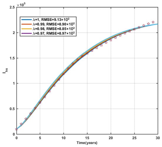
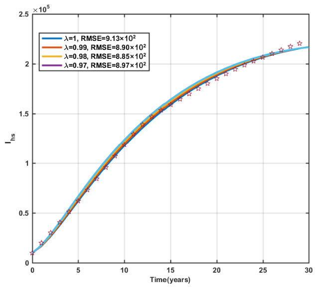
The fractional order $\lambda$ is varied to get Figure 4. The RMSE for each value of $\lambda$ is given in Table 4. When the fractional order $\lambda$ equals 0.98, the least root-mean-square error is obtained. We will use this fractional order value to perform numerical simulations of the fractional model (7).

Figure 4. Comparison of cumulative cases denoted by stars and cases predicted by the model for different values of $\lambda$.

Table 4. The related RMSE for fractional order $\lambda$.

$\mathit{\lambda }$	RMSE	$\mathit{\lambda }$	RMSE
1	913.2	0.98	885.8
0.99	890.8	0.97	897.9

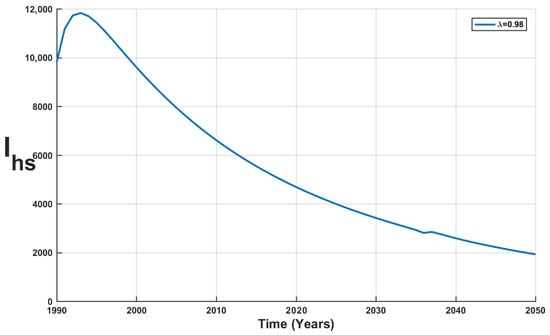
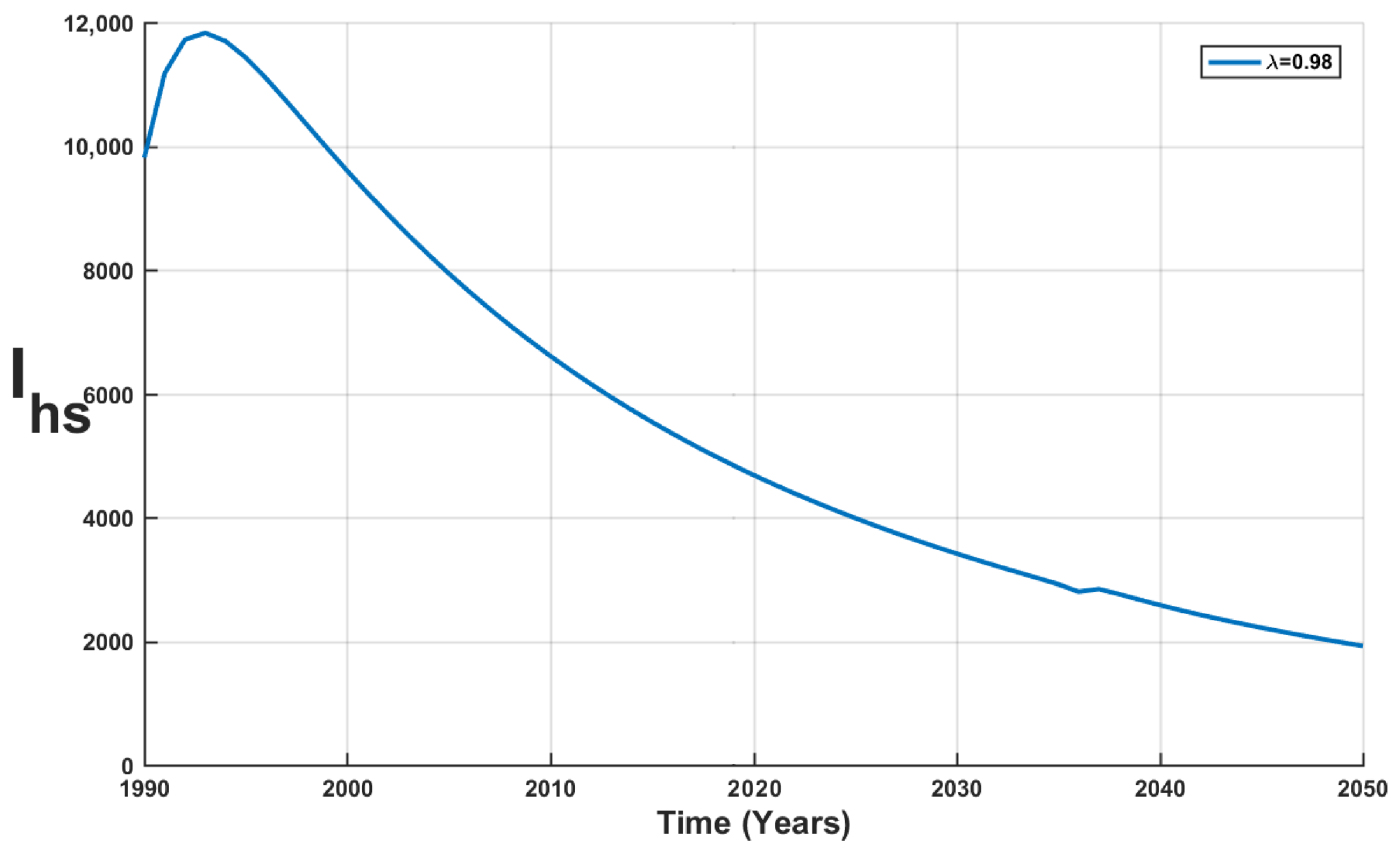
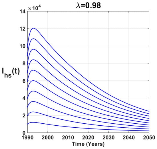
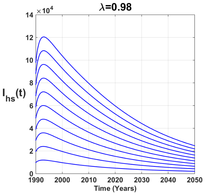
We studied real-time data from Cameroon and found that using Caputo’s fractional derivative to study the data more clearly predicts epidemic peaks at different values of fractional order $\lambda$. The parameter values used here are presented in Table 3, for which the basic reproduction number $R_0$ is equal to 1.169. For the fractional order $\lambda =0.98$ with different initial conditions, we obtained the prediction figure for first-stage trachoma from 2019 to 2050 (see Figure 5). We note that, in the 1990s, there were around 10,000 individuals infected with the first stage of trachoma. From 1990 to 1995, there was a slight increase in $I_{hs}$ to around 12,000. From 2005 to 2019, $I_{hs}$ gradually decreased from around 4400.

Figure 5. Prediction of first-stage trachoma new cases from 2019 to 2050.

5.2. Strength Number and Epidemic Waves

The basic reproduction number is the central concept in the analysis of epidemiological models. In fact, it influences how epidemiological systems behave qualitatively. Using the same arguments as in [53,54], we will compute the strength number of model (5). Note that

$$\begin{array}{cc}\hfill {\displaystyle \frac{{\partial }^2}{\partial I_v^2}}\left(a_h^{\lambda }{b}_v^{\lambda }{\displaystyle \frac{S_h{I}_v}{1+{\psi }_1{I}_v}}+{\nu }^{\lambda }{\displaystyle \frac{S_{h}B}{B+K}}\right)& =-{\displaystyle \frac{2a_h^{\lambda }{b}_v^{\lambda }{\psi }_1{S}_h}{{(1+{\psi }_1{I}_v)}^3}},\hfill \\ \hfill {\displaystyle \frac{{\partial }^2}{\partial B^2}}\left(a_h^{\lambda }{b}_v^{\lambda }{\displaystyle \frac{S_h{I}_v}{1+{\psi }_1{I}_v}}+{\nu }^{\lambda }{\displaystyle \frac{S_{h}B}{B+K}}\right)& =-{\displaystyle \frac{2{\nu }_h^{\lambda }K{S}_h}{{(K+B)}^3}},\hfill \\ \hfill {\displaystyle \frac{{\partial }^2}{\partial I_{hs}^2}}\left(a_v^{\lambda }{b}_v^{\lambda }{\displaystyle \frac{S_v\left(I_{hs}+I_{hc}\right)}{1+{\psi }_2\left(I_{hs}+I_{hc}\right)}}\right)& =-{\displaystyle \frac{2{\psi }_2{a}_v^{\lambda }{b}_v^{\lambda }{S}_v}{{(1+{\psi }_2\left(I_{hs}+I_{hc}\right))}^3}},\hfill \\ \hfill {\displaystyle \frac{{\partial }^2}{\partial I_{hc}^2}}\left(a_v^{\lambda }{b}_v^{\lambda }{\displaystyle \frac{S_v\left(I_{hs}+I_{hc}\right)}{1+{\psi }_2\left(I_{hs}+I_{hc}\right)}}\right)& =-{\displaystyle \frac{2{\psi }_2{a}_v^{\lambda }{b}_v^{\lambda }{S}_v}{{(1+{\psi }_2\left(I_{hs}+I_{hc}\right))}^3}}.\hfill \end{array}$$

At the trachoma-free equilibrium $x_0$, we obtain

$$\begin{array}{cc}\hfill {\left.{\displaystyle \frac{{\partial }^2}{\partial I_v^2}}\left(a_h^{\lambda }{b}_v^{\lambda }{\displaystyle \frac{S_h{I}_v}{1+{\psi }_1{I}_v}}+{\nu }^{\lambda }{\displaystyle \frac{S_{h}B}{B+K}}\right)\right|}_{x_0}& =-2{\psi }_1{a}_h^{\lambda }{b}_v^{\lambda }{S}_{h0},\hfill \\ \hfill {\left.{\displaystyle \frac{{\partial }^2}{\partial B^2}}\left(a_h^{\lambda }{b}_v^{\lambda }{\displaystyle \frac{S_h{I}_v}{1+{\psi }_1{I}_v}}+{\nu }^{\lambda }{\displaystyle \frac{S_{h}B}{B+K}}\right)\right|}_{x_0}& =-{\displaystyle \frac{2{\nu }_h^{\lambda }{S}_{h0}}{K^2}},\hfill \\ \hfill {\left.{\displaystyle \frac{{\partial }^2}{\partial I_{hs}^2}}\left(a_v^{\lambda }{b}_v^{\lambda }{\displaystyle \frac{S_v\left(I_{hs}+I_{hc}\right)}{1+{\psi }_2\left(I_{hs}+I_{hc}\right)}}\right)\right|}_{x_0}& =-2{\psi }_2{a}_v^{\lambda }{b}_v^{\lambda }{S}_{v0}={\left.{\displaystyle \frac{{\partial }^2}{\partial I_{hc}^2}}\left(a_v^{\lambda }{b}_v^{\lambda }{\displaystyle \frac{S_v\left(I_{hs}+I_{hc}\right)}{1+{\psi }_2\left(I_{hs}+I_{hc}\right)}}\right)\right|}_{x_0}.\hfill \end{array}$$

We thus have $F_A:=\left(\begin{array}{cccccc}0& 0& 0& 0& -2{\psi }_1{a}_h^{\lambda }{b}_v^{\lambda }{S}_{h0}& -{\displaystyle \frac{2{\nu }_h^{\lambda }{S}_{h0}}{K^2}}\\ 0& 0& 0& 0& 0& 0\\ 0& 0& 0& 0& 0& 0\\ 0& -2{\psi }_2{a}_v^{\lambda }{b}_v^{\lambda }{S}_{v0}& -2{\psi }_2{a}_v^{\lambda }{b}_v^{\lambda }{S}_{v0}& 0& 0& 0\\ 0& 0& 0& 0& 0& 0\\ 0& 0& 0& 0& 0& 0\end{array}\right)$ and

$V:={\mathcal{J}}_{\mathcal{V}}\left(TFE\right)=\left(\begin{array}{cccccc}-w_1& 0& 0& 0& 0& 0\\ {\gamma }_1^{\lambda }& -w_2& 0& 0& 0& 0\\ 0& {\gamma }_2^{\lambda }& -w_3& 0& 0& 0\\ 0& 0& 0& -w_5& 0& 0\\ 0& 0& 0& {\tau }^{\lambda }& -{\mu }_v^{\lambda }& 0\\ 0& {\kappa }_1^{\lambda }& {\kappa }_2^{\lambda }& 0& {\kappa }_3^{\lambda }& -{\mu }_b^{\lambda }\end{array}\right)$ where

$$\begin{array}{cc}\hfill w_1^{\lambda }:=& {\gamma }_1^{\lambda }+{\theta }_1^{\lambda }+{\mu }_h^{\lambda },w_2^{\lambda }:={\gamma }_2^{\lambda }+{\theta }_2^{\lambda }+{\mu }_h^{\lambda },w_3^{\lambda }:={\theta }_3^{\lambda }+{\mu }_h^{\lambda },w_5^{\lambda }:={\tau }^{\lambda }+{\mu }_v^{\lambda }.\hfill \end{array}$$

From [53], we get that the strength number is equal to the spectral radius of $-F_A{V}^{-1}$. $-F_A{V}^{-1}$ is given by $P\left(y\right)=z_2{y}^2+z_{1}y+z_0$ representing the characteristic polynomial where

$$\begin{array}{cc}\hfill z_2& =w_1{w}_2{w}_3{w}_5{K}^2{\mu }_b{\mu }_v,\hfill \\ \hfill z_1& =\left(2{\gamma }_1{\kappa }_1{w}_3+2{\gamma }_1{\gamma }_2{\kappa }_2\right)w_5{S}_{\mathit{h}\mathit{0}}\nu {\mu }_v,\hfill \\ \hfill z_0& =-4{\gamma }_1{\psi }_2\left(w_3+{\gamma }_2\right)S_{\mathit{h}\mathit{0}}{a}_v{b}_v\left({\psi }_1{K}^2{\mu }_b{a}_h{b}_v+{\kappa }_{3}nu\right)S_{\mathit{v}\mathit{0}}\tau .\hfill \end{array}$$

Since $z_2$ and $z_1$ are always positive while $z_0$ is always negative, it follows that $D=z_1^2-4z_2{z}_0>0$. This means that the spectral radius of $F_A{V}^{-1}$ is the positive root of P(y), which is called the strength number. It thus follows from [53] (see also [54]), that trachoma model (5) can admits multiple epidemic waves.

5.3. Uncertainty and Global Sensitivity Analysis

Partial rank correlation coefficients (PRCCs) between the fundamental reproduction number ${\mathcal{R}}_0$ and each parameter are obtained using 10,000 runs of the Latin hypercube sampling (LHS) method [55], in accordance with the methodology of Marino et al. [56] and Wu et al. [57]. Table 3 lists the mean values of the parameters, which are considered to be random variables with uniform distributions [58].

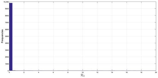
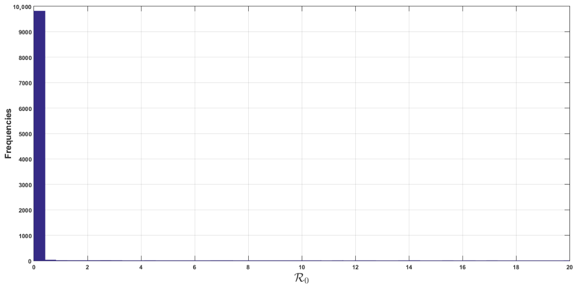
Figure 6 shows the derived distribution of ${\mathcal{R}}_0$ using these 10,000 LHS runs. According to this sampling, the standard deviation is 1.7910 and the mean of ${\mathcal{R}}_0$ is 1.1961. This suggests that we may be certain that the model predicts an endemic condition for the mean of the parameter values listed in Table 3.

Figure 6. Sampling distribution of ${\mathcal{R}}_0$ from 10,000 runs of Latin hypercube sampling. The mean of ${\mathcal{R}}_0$ is 1.1961 and the standard deviation is 1.7910.

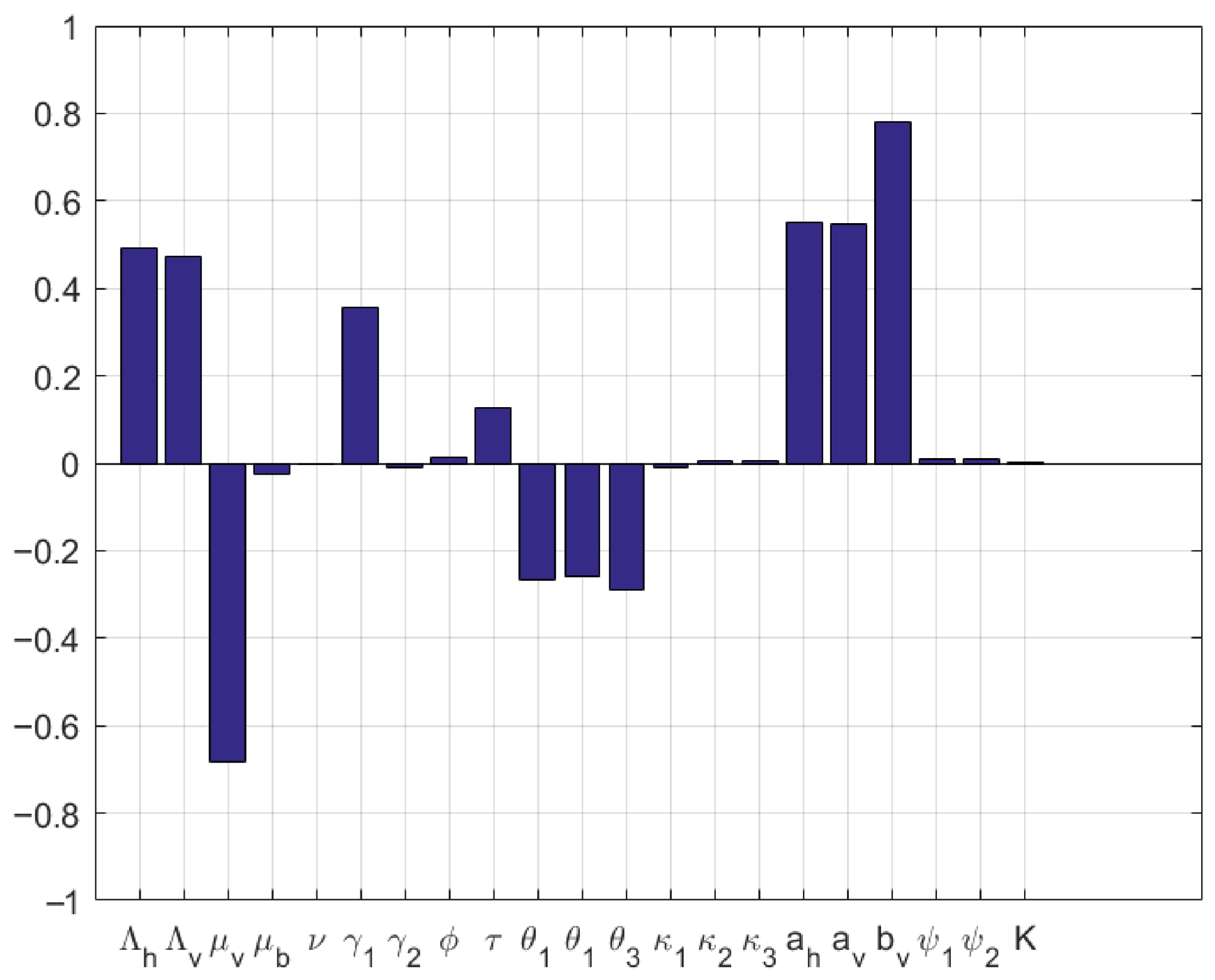
In the following, we analyze the impact of various parameters on ${\mathcal{R}}_0$ through global sensitivity analysis, calculating the partial rank correlation coefficient (PRCC) between ${\mathcal{R}}_0$ and each model parameter, with $\lambda =1$. The findings are illustrated in Figure 7. It follows that parameters ${\Lambda }_h$, ${\Lambda }_v$, ${\mu }_v$, $a_h$, $a_v$ and $b_v$ are the most important in the dynamics of the trachoma model. Indeed, the PRCCs of these parameter are comprised in the interval $[-1;-0.5]\cup [+0.5;1]$ [57].

Figure 7. PRCC between ${\mathcal{R}}_0$ and each model parameter (we set $\varphi :=\phi$).

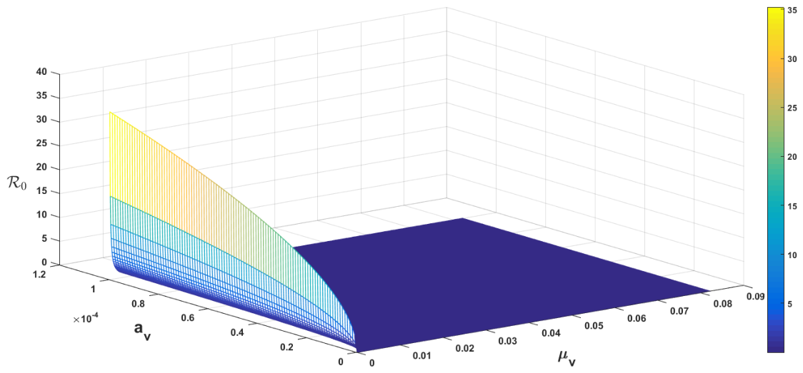
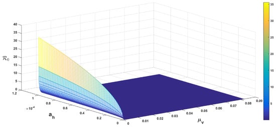
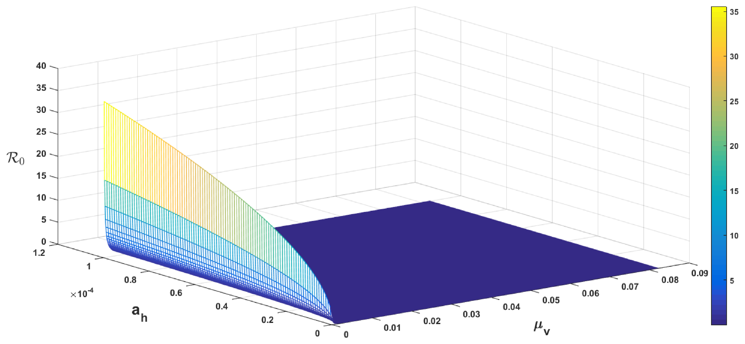
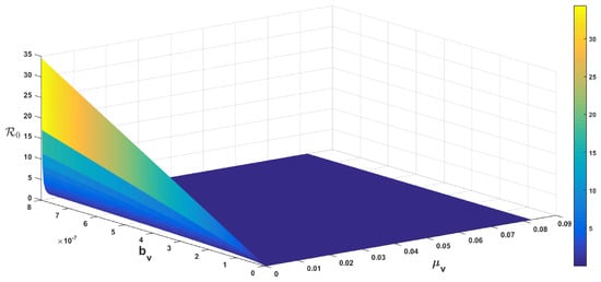
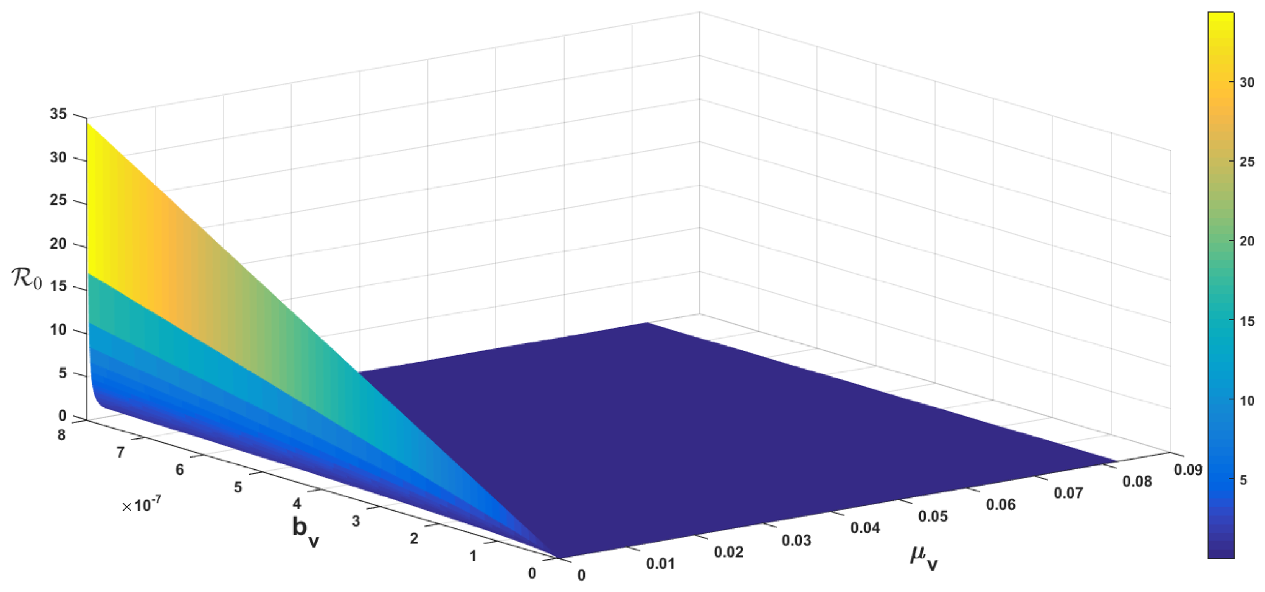
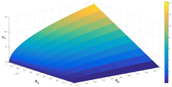
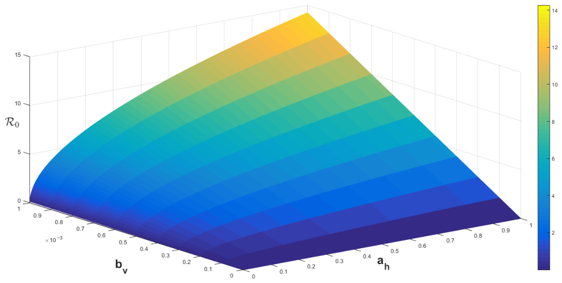
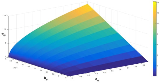
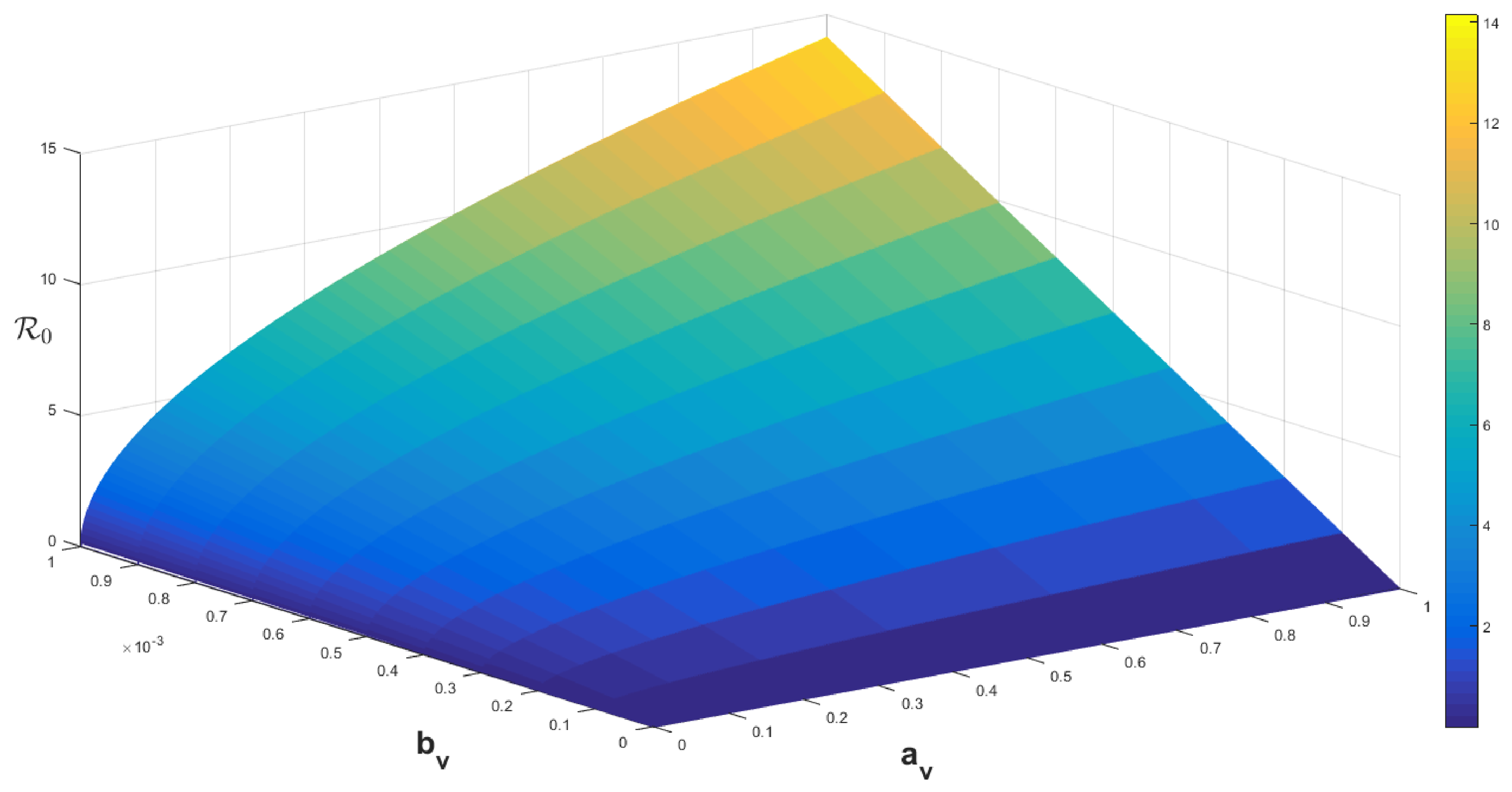
Figure 8, Figure 9, Figure 10, Figure 11 and Figure 12 display the variation in ${\mathcal{R}}_0$ in terms of the most important model parameters ${\mu }_v$, $a_h$, $a_v$, and $b_v$. It is evident that reducing $a_h$, $a_v$, and $b_v$ and increasing the rate of fly mortality ${\mu }_v$ through increased vector control and personal protection can help curb the spread of trachoma in the human population.

Figure 8. ${\mathcal{R}}_0$ in terms of ${\mu }_v$ and $a_v$ plotted in three dimensions.

Figure 9. ${\mathcal{R}}_0$ in terms of ${\mu }_v$ and $a_h$ plotted in three dimensions.

Figure 10. ${\mathcal{R}}_0$ in terms of ${\mu }_v$ and $b_v$ plotted in three dimensions.

Figure 11. ${\mathcal{R}}_0$ in term of $a_h$ and $b_v$ plotted in three dimensions.

Figure 12. ${\mathcal{R}}_0$ in term of $a_v$ and $b_v$ plotted in three dimensions.

6. Numerical Scheme and Its Stability

6.1. Model Solution and Stability of the Numerical Scheme

The use of numerical methods and approximation is necessary because most fractional systems do not admit exact analytical solutions [59,60]. Therefore, various numerical methods have been developed to effectively examine and simulate the dynamics of such systems, as discussed in [61,62]. Fractional-order differential equations can be solved using various analytical and numerical methods [63,64]. The generalized Adams–Bashforth–Moulton method can be used for numerical solutions of system (5). We consider the following nonlinear fractional-order differential problem to find an exact solution with this approach [65]:

$$\left\{\begin{array}{cc}{\mathcal{D}}_t^{\lambda }h\left(t\right)\hfill & =g(t,h(t\left)\right),0\le t\le T\hfill \\ h^{\left(k\right)}\left(0\right)\hfill & =h_0^{\left(k\right)},k=0,1,2,...,m-1,\mathrm{or}m=\left[\lambda \right]\hfill \end{array}\right.$$

(37)

This equation is equivalent to the Volterra integral equation:

$h\left(t\right)={\displaystyle \sum _{k=0}^{m-1}}{h}_0^{\left(k\right)}{\displaystyle \frac{t^k}{k!}}+{\displaystyle \frac{1}{\Gamma \left(\lambda \right)}}{\int }_0^t{(t-s)}^{\lambda -1}g(s,h\left(s\right))ds$.

Diethelm and Neville [66] employed the Adams–Bashforth–Moulton algorithm-based predictor–corrector method [67]. We therefore use the same technique again to find the solution of model (5). For $\lambda \in [0,1]$, $0\le t\le T$ and setting $h={\displaystyle \frac{T}{N}}$ and $t_n=nh$, for $n=0,1,2,...,N$$\in {\mathbb{Z}}^{+}$, the model solution is

$$\begin{array}{cc}\hfill S_{h(n+1)}& =S_{h0}+{\displaystyle \frac{h^{\lambda }}{\Gamma (\lambda +2)}}\left({\Lambda }_h^{\lambda }-({\alpha }_h^{\lambda }+{\alpha }_i^{\lambda })S_{h(n+1)}^p+{\phi }^{\lambda }{R}_{h(n+1)}^p-{\mu }_h^{\lambda }{S}_{h(n+1)}^p\right)\hfill \\ \hfill & +{\displaystyle \frac{h^{\lambda }}{\Gamma (\lambda +2)}}\sum _{j=0}^n{b}_{j,n+1}\left({\Lambda }_h^{\lambda }-({\alpha }_h^{\lambda }+{\alpha }_i^{\lambda })S_{h\left(j\right)}+{\phi }^{\lambda }{R}_{h\left(j\right)}-{\mu }_h^{\lambda }{S}_{h\left(j\right)}\right),\hfill \\ \hfill E_{h(n+1)}& =E_{h0}+{\displaystyle \frac{h^{\lambda }}{\Gamma (\lambda +2)}}\left(({\alpha }_h^{\lambda }+{\alpha }_i^{\lambda })S_{h(n+1)}^p-{\gamma }_1^{\lambda }{E}_{h(n+1)}^p-{\mu }_h^{\lambda }{E}_{h(n+1)}^p-{\theta }_1^{\lambda }{E}_{h(n+1)}^p\right)\hfill \\ \hfill & +{\displaystyle \frac{h^{\lambda }}{\Gamma (\lambda +2)}}\sum _{j=0}^n{b}_{j,n+1}\left(({\alpha }_h^{\lambda }+{\alpha }_i^{\lambda })S_{h\left(j\right)}-{\gamma }_1^{\lambda }{E}_{h\left(j\right)}-{\mu }_h^{\lambda }{E}_{h\left(j\right)}-{\theta }_1^{\lambda }{E}_{h\left(j\right)}\right),\hfill \\ \hfill I_{hs(n+1)}& =I_{hs0}+{\displaystyle \frac{h^{\lambda }}{\Gamma (\lambda +2)}}\left({\gamma }_1^{\lambda }{E}_{h(n+1)}^p-{\gamma }_2^{\lambda }{I}_{hs(n+1)}^p-{\mu }_h^{\lambda }{I}_{hs(n+1)}^p-{\theta }_2^{\lambda }{I}_{hs(n+1)}^p\right)\hfill \\ \hfill & +{\displaystyle \frac{h^{\lambda }}{\Gamma (\lambda +2)}}\sum _{j=0}^n{b}_{j,n+1}\left({\gamma }_1^{\lambda }{E}_{h\left(j\right)}-{\gamma }_2^{\lambda }{I}_{hs\left(j\right)}-{\mu }_h^{\lambda }{I}_{hs\left(j\right)}-{\theta }_2^{\lambda }{I}_{hs\left(j\right)}\right),\hfill \\ \hfill I_{hc(n+1)}& =I_{hc0}+{\displaystyle \frac{h^{\lambda }}{\Gamma (\lambda +2)}}\left({\gamma }_2^{\lambda }{I}_{hs(n+1)}^p-{\theta }_3^{\lambda }{I}_{hc(n+1)}^p-{\mu }_h^{\lambda }{I}_{hc(n+1)}^p\right)\hfill \\ \hfill & +{\displaystyle \frac{h^{\lambda }}{\Gamma (\lambda +2)}}\sum _{j=0}^n{b}_{j,n+1}\left({\gamma }_2^{\lambda }{I}_{hs\left(j\right)}-{\theta }_3^{\lambda }{I}_{hc\left(j\right)}-{\mu }_h^{\lambda }{I}_{hc\left(j\right)}\right),\hfill \\ \hfill R_{h(n+1)}& =S_{h0}+{\displaystyle \frac{h^{\lambda }}{\Gamma (\lambda +2)}}\left({\theta }_1^{\lambda }{E}_{h(n+1)}^p+{\theta }_2^{\lambda }{I}_{hs(n+1)}^p+{\theta }_3^{\lambda }{I}_{hc(n+1)}^p-{\phi }^{\lambda }{R}_{h(n+1)}^p-{\mu }_h^{\lambda }{R}_{h(n+1)}^p\right)\hfill \\ \hfill & +{\displaystyle \frac{h^{\lambda }}{\Gamma (\lambda +2)}}\sum _{j=0}^n{b}_{j,n+1}\left({\theta }_1^{\lambda }{E}_{h\left(j\right)}+{\theta }_2^{\lambda }{I}_{hs\left(j\right)}+{\theta }_3^{\lambda }{I}_{hc\left(j\right)}-{\phi }^{\lambda }{R}_{h\left(j\right)}-{\mu }_h^{\lambda }{R}_{h\left(j\right)}\right),\hfill \end{array}$$

(38)

$$\begin{array}{cc}\hfill S_{v(n+1)}& =S_{v0}+{\displaystyle \frac{h^{\lambda }}{\Gamma (\lambda +2)}}\left({\Lambda }_v^{\lambda }-{\alpha }_v^{\lambda }{S}_{v(n+1)}^p-{\mu }_v^{\lambda }{S}_{v(n+1)}^p\right)\hfill \\ \hfill & +{\displaystyle \frac{h^{\lambda }}{\Gamma (\lambda +2)}}\sum _{j=0}^n{b}_{j,n+1}\left({\Lambda }_v^{\lambda }-{\alpha }_v^{\lambda }{S}_{v\left(j\right)}-{\mu }_v^{\lambda }{S}_{v\left(j\right)}\right),\hfill \\ \hfill E_{v(n+1)}& =E_{v0}+{\displaystyle \frac{h^{\lambda }}{\Gamma (\lambda +2)}}\left({\alpha }_v^{\lambda }{S}_{v(n+1)}^p-{\tau }^{\lambda }{E}_{v(n+1)}^p-{\mu }_v^{\lambda }{E}_{v(n+1)}^p\right)\hfill \\ \hfill & +{\displaystyle \frac{h^{\lambda }}{\Gamma (\lambda +2)}}\sum _{j=0}^n{b}_{j,n+1}\left({\alpha }_v^{\lambda }{S}_{v\left(j\right)}-{\tau }^{\lambda }{E}_{v\left(j\right)}-{\mu }_v^{\lambda }{E}_{vj}\right),\hfill \\ \hfill I_{v(n+1)}& =I_{v0}+{\displaystyle \frac{h^{\lambda }}{\Gamma (\lambda +2)}}\left({\tau }^{\lambda }{E}_{v(n+1)}^p-{\mu }_v^{\lambda }{I}_{v(n+1)}^p\right)+{\displaystyle \frac{h^{\lambda }}{\Gamma (\lambda +2)}}\sum _{j=0}^n{b}_{j,n+1}\left({\tau }^{\lambda }{E}_{v\left(j\right)}^{\lambda }-{\mu }_v^{\lambda }{I}_{v\left(j\right)}\right),\hfill \\ \hfill B_{n+1}& =B_0+{\displaystyle \frac{h^{\lambda }}{\Gamma (\lambda +2)}}\left({\kappa }_1^{\lambda }{I}_{hs(n+1)}^p+{\kappa }_2^{\lambda }{I}_{hc(n+1)}^p+{\kappa }_3^{\lambda }{I}_{v(n+1)}^p-{\mu }_b^{\lambda }B\right)\hfill \\ \hfill & +{\displaystyle \frac{h^{\lambda }}{\Gamma (\lambda +2)}}\sum _{j=0}^n{b}_{j,n+1}\left({\kappa }_1^{\lambda }{I}_{hs\left(j\right)}+{\kappa }_2^{\lambda }{I}_{hc\left(j\right)}+{\kappa }_3^{\lambda }{I}_{v\left(j\right)}-{\mu }_b^{\lambda }{B}_j\right),\hfill \end{array}$$

(39)

where

$$\begin{array}{cc}\hfill S_{h(n+1)}^p& =S_{h0}+{\displaystyle \frac{h^{\lambda }}{\Gamma \left(\lambda \right)}}\sum _{j=0}^n{d}_{j,n+1}\left({\Lambda }_h^{\lambda }-({\alpha }_h^{\lambda }+{\alpha }_i^{\lambda })S_{h\left(j\right)}+{\phi }^{\lambda }{R}_{h\left(j\right)}-{\mu }_h^{\lambda }{S}_{h\left(j\right)}\right),\hfill \\ \hfill E_{hn+1}^p& =E_{h0}+{\displaystyle \frac{h^{\lambda }}{\Gamma \left(\lambda \right)}}\sum _{j=0}^n{d}_{j,n+1}\left(({\alpha }_h^{\lambda }+{\alpha }_i^{\lambda })S_{h\left(j\right)}-{\gamma }_1^{\lambda }{E}_{h\left(j\right)}-{\mu }_h^{\lambda }{E}_{h\left(j\right)}-{\theta }_1^{\lambda }{E}_{h\left(j\right)}\right),\hfill \\ \hfill I_{hs(n+1)}^p& =I_{hs0}+{\displaystyle \frac{h^{\lambda }}{\Gamma \left(\lambda \right)}}\sum _{j=0}^n{d}_{j,n+1}\left({\gamma }_1^{\lambda }{E}_{h\left(j\right)}-{\gamma }_2^{\lambda }{I}_{hs\left(j\right)}-{\mu }_h^{\lambda }{I}_{hs\left(j\right)}-{\theta }_2^{\lambda }{I}_{hsj}\right),\hfill \\ \hfill I_{hc(n+1)}^p& =I_{hc0}+{\displaystyle \frac{h^{\lambda }}{\Gamma \left(\lambda \right)}}\sum _{j=0}^n{d}_{j,n+1}\left({\gamma }_2^{\lambda }{I}_{hs\left(j\right)}-{\theta }_3^{\lambda }{I}_{hc\left(j\right)}-{\mu }_h^{\lambda }{I}_{hc\left(j\right)}\right),\hfill \\ \hfill R_{h(n+1)}^p& =R_{h0}+{\displaystyle \frac{h^{\lambda }}{\Gamma (\lambda +2)}}\sum _{j=0}^n{d}_{j,n+1}\left({\theta }_1^{\lambda }{E}_{h\left(j\right)}+{\theta }_2^{\lambda }{I}_{hs\left(j\right)}+{\theta }_3^{\lambda }{I}_{hc\left(j\right)}-{\phi }^{\lambda }{R}_{h\left(j\right)}-{\mu }_h^{\lambda }{R}_{h\left(j\right)}\right),\hfill \\ \hfill S_{v(n+1)}^p& =S_{v0}+{\displaystyle \frac{h^{\lambda }}{\Gamma \left(\lambda \right)}}\sum _{j=0}^n{d}_{j,n+1}\left({\Lambda }_v^{\lambda }-{\alpha }_v^{\lambda }{S}_{v\left(j\right)}-{\mu }_v^{\lambda }{S}_{v\left(j\right)}\right),\hfill \\ \hfill E_{v(n+1)}^p& =E_{v0}+{\displaystyle \frac{h^{\lambda }}{\Gamma \left(\lambda \right)}}\sum _{j=0}^n{d}_{j,n+1}\left({\alpha }_v^{\lambda }{S}_{v\left(j\right)}-{\tau }^{\lambda }{E}_{v\left(j\right)}-{\mu }_v^{\lambda }{E}_{v\left(j\right)}\right),\hfill \\ \hfill I_{v(n+1)}^p& =I_{v0}+{\displaystyle \frac{h^{\lambda }}{\Gamma \left(\lambda \right)}}\sum _{j=0}^n{d}_{j,n+1}\left({\tau }^{\lambda }{E}_{v\left(j\right)}-{\mu }_v^{\lambda }{I}_{v\left(j\right)}\right),\hfill \\ \hfill B_{n+1}^p& =B_0+{\displaystyle \frac{h^{\lambda }}{\Gamma \left(\lambda \right)}}\sum _{j=0}^n{d}_{j,n+1}\left({\kappa }_1^{\lambda }{I}_{hs\left(j\right)}+{\kappa }_2^{\lambda }{I}_{hc\left(j\right)}+{\kappa }_3^{\lambda }{I}_{v\left(j\right)}-{\mu }_b^{\lambda }{B}_{\left(j\right)}\right),\hfill \end{array}$$

(40)

and

$$b_{j,n+1}=\left\{\begin{array}{c}{n}^{\lambda +1}-(n-\lambda )(n+1),j=0,\hfill \\ {(n-j+2)}^{\lambda +1}-2{(n-j+1)}^{\lambda +1}+{(n-j)}^{\lambda +1}1\le j\le n,\hfill \\ 1,j=n+1,\hfill \end{array}\right.$$

$d_{j,n+1}={\displaystyle \frac{h^{\lambda }}{\lambda }}\left({(n-j+1)}^{\lambda }-{(n-1)}^{\lambda }\right),0\le j\le n$

Theorem 12.

The numerical scheme (38)–(40) is conditionally stable.

Proof. 

Let ${\tilde{S}}_{h0}$, ${\tilde{S}}_{h\left(j\right)}(j=0,...,n+1)$ and ${\tilde{S}}_{hn+1}^p(n=0,...,N-1)$ be disrupters of $S_{h0}$, $S_{h\left(j\right)}$ and $S_{hn+1}^p$, respectively. The following disturbance equations are obtained using Equations (40)–(42) defined below:

$${\tilde{S}}_{h(n+1)}^p={\tilde{S}}_{h0}+{\displaystyle \frac{h^{\lambda }}{\Gamma \left(\lambda \right)}}\sum _{j=0}^n{d}_{j,n+1}\left(F_1(t_j,S_{h\left(j\right)}+{\tilde{S}}_{h\left(j\right)})-F_1(t_j,S_{h\left(j\right)})\right),$$

(41)

$$\begin{array}{c}\hfill {\tilde{S}}_{h(n+1)}={\tilde{S}}_{h0}+{\displaystyle \frac{h^{\lambda }}{\Gamma (\lambda +2)}}\left(F_1(t_{n+1},S_{h(n+1)}^p+{\tilde{S}}_{h(n+1)}^p)-F_1(t_{n+1},S_{h(n+1)}^p)\right)\\ \hfill +{\displaystyle \frac{h^{\lambda }}{\Gamma (\lambda +2)}}\sum _{j=0}^n{b}_{j,n+1}\left(F_1(t_j,S_{h\left(j\right)}+{\tilde{S}}_{h\left(j\right)})-F_1(t_j,S_{h\left(j\right)})\right),\end{array}$$

(42)

Using the Lipschitz condition, we obtain

$$\left|{\tilde{S}}_{h(n+1)}\right|\le {\zeta }_0+{\displaystyle \frac{h^{\lambda }{L}_1}{\Gamma (\lambda +2)}}\left(\left|{\tilde{S}}_{h(n+1)}^p\right|+\sum _{j=1}^n{b}_{j,n+1}\left|{\tilde{S}}_{h\left(j\right)}\right|\right)$$

(43)

where ${\zeta }_0=\underset{0\le n\le N}{max}\left\{\left|{\tilde{S}}_{h0}^p\right|+{\displaystyle \frac{h^{\lambda }{L}_1{b}_{n,0}}{\Gamma (\lambda +2)}}\left|{\tilde{S}}_{h0}\right|\right\}.$

Furthermore, from ([68], Equation (3.18)), we derive

$$\left|{\tilde{S}}_{h(n+1)}^p\right|\le {\eta }_0+{\displaystyle \frac{L_1}{\Gamma \left(\lambda \right)}}\sum _{j=1}^n{d}_{j,n+1}\left|{\tilde{S}}_{hj}\right|$$

(44)

where ${\eta }_0=\underset{0\le n\le N}{max}\left\{\left|{\tilde{S}}_{h0}^p\right|+{\displaystyle \frac{h^{\lambda }{L}_1{d}_{n,0}}{\Gamma \left(\lambda \right)}}\left|{\tilde{S}}_{h0}\right|\right\}$.

Substituting ${\tilde{S}}_{h0}^p$ from Equation (44) into Equation (43) we have

$$\begin{array}{cc}\hfill \left|{\tilde{S}}_{h(n+1)}^p\right|\le & {ϵ}_0+{\displaystyle \frac{h^{\lambda }{L}_1}{\Gamma (\lambda +2)}}\left({\displaystyle \frac{L_1}{\Gamma \left(\lambda \right)}}\sum _{j=1}^n{d}_{j,n+1}\left|{\tilde{S}}_{h\left(j\right)}\right|+\sum _{j=1}^n{b}_{j,n+1}\left|{\tilde{S}}_{h\left(j\right)}\right|\right)\hfill \\ \hfill \le & {ϵ}_0+{\displaystyle \frac{h^{\lambda }{L}_1}{\Gamma (\lambda +2)}}\sum _{j=1}^n\left({\displaystyle \frac{L_1}{\Gamma \left(\lambda \right)}}{d}_{j,n+1}+b_{j,n+1}\right)\left|{\tilde{S}}_{h\left(j\right)}\right|\hfill \\ \hfill \le & {ϵ}_0+{\displaystyle \frac{h^{\lambda }{L}_1{E}_{\lambda ,2}}{\Gamma (\lambda +2)}}\sum _{j=1}^n{\left(n+1-j\right)}^{\lambda -1}\left|{\tilde{S}}_{h\left(j\right)}\right|,\hfill \end{array}$$

(45)

where ${ϵ}_0=\underset{0\le n\le N}{max}\left\{{\zeta }_0+{\displaystyle \frac{h^{\lambda }{L}_1{b}_{n+1,n+1}}{\Gamma (\lambda +2)}}{\eta }_0\right\}.$$E_{\lambda ,2}$ is a positive constant that depends only on $\lambda$ (see [69], Lemma 2) and h is assumed to be sufficiently small. The application of ([69], Lemma 1) permits concluding that ${\tilde{S}}_{h(n+1)}^p\le E{ϵ}_0$. □

6.2. Numerical Results and Discussion

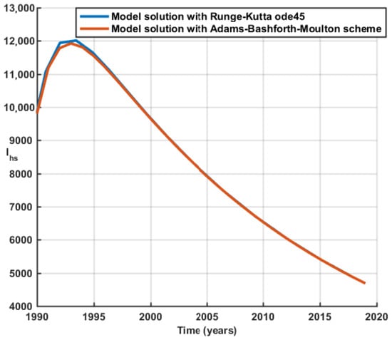
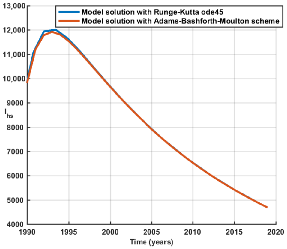
Figure 13 shows the model solution obtained using two different methods (Runge–Kutta of order 4 and the Adams–Bashforth–Moulton scheme) for $\lambda =1$. We see that the solution obtained with Runge–Kutta of order 4 match the one obtained with the Adams–Bashforth–Moulton scheme.

Figure 13. Model solution using two simulation methods for the case $\lambda =1$.

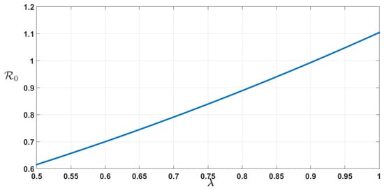
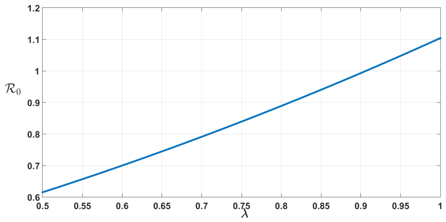
Figure 14 depicts the graph of ${\mathcal{R}}_0$ as a function of the fractional-order $\lambda$. The parameter values are those of Table 3. It is clear that ${\mathcal{R}}_0$ is a decreasing function of $\lambda$.

Figure 14. ${\mathcal{R}}_0$ plotted in two dimensions as a function of the fractional-order $\lambda$. The parameter values are those of Table 3.

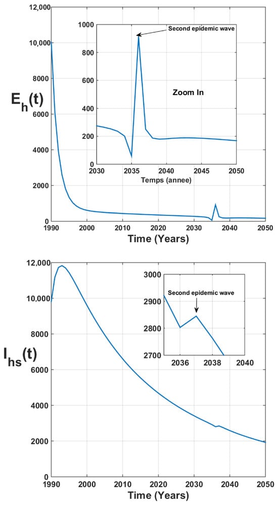
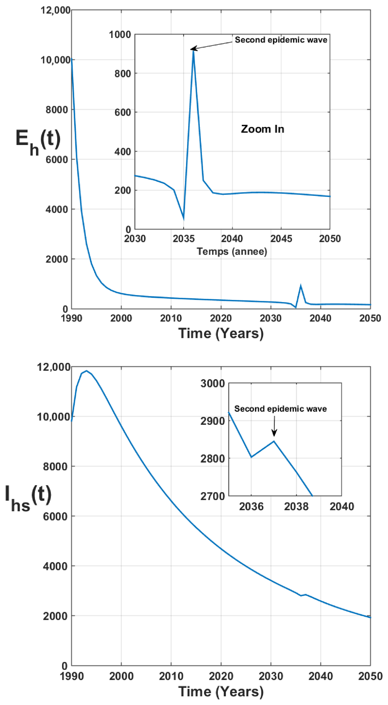
Figure 15 depicts the possibility of multiple epidemic waves of trachoma. Indeed, we clearly see that, around the year 2040, another peak could appear. This can be justified by waning immunity [70] or seasonal fly population spikes [71].

Figure 15. Forecasting of the first stage of the trachoma disease $Ihs$ with values as in Table 3.

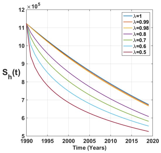
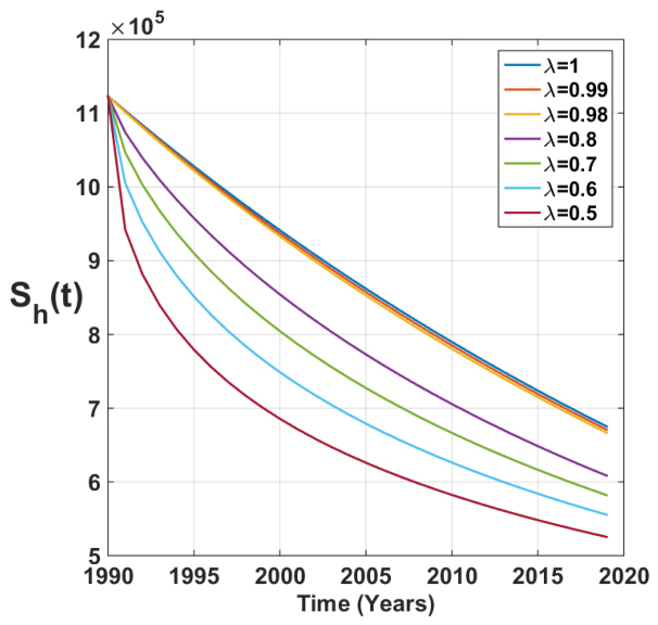
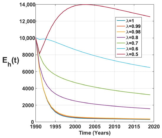
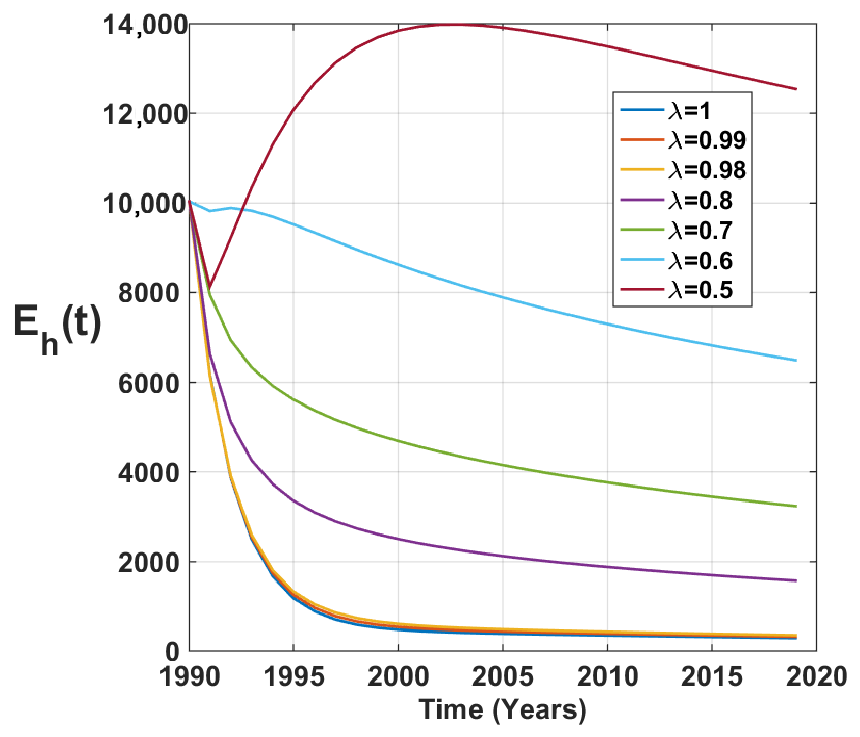
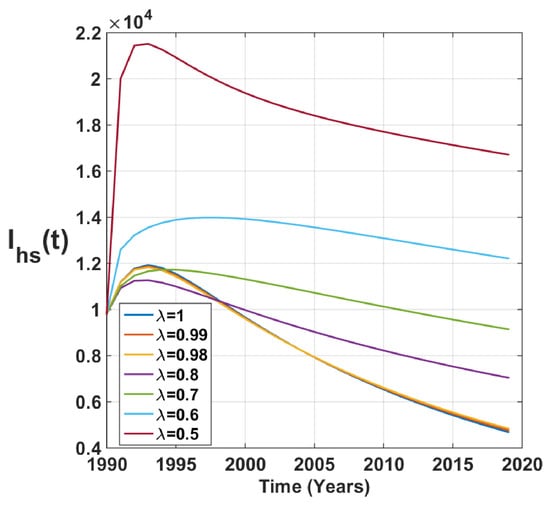
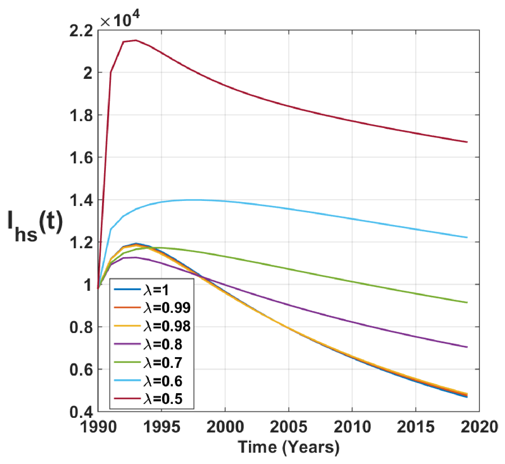
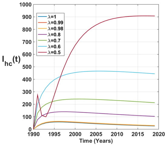
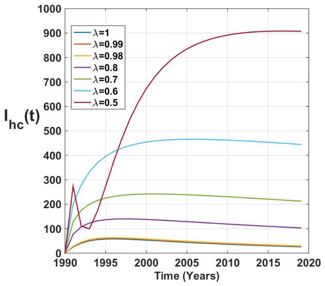
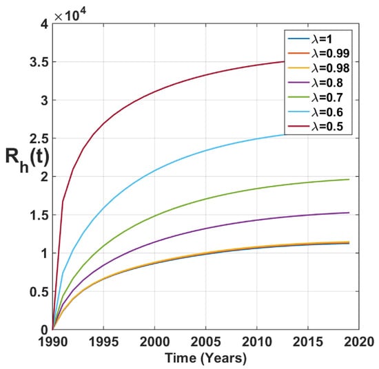
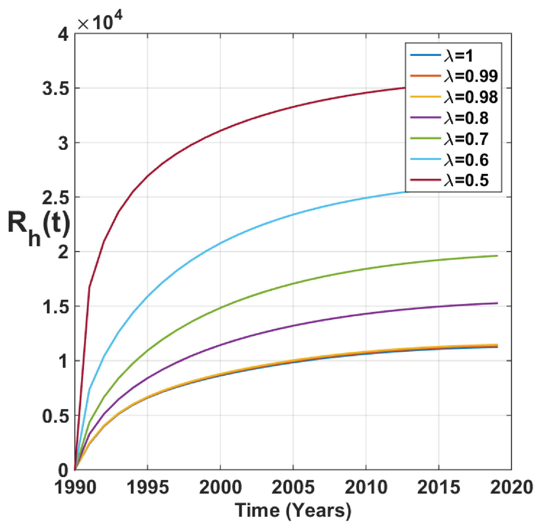
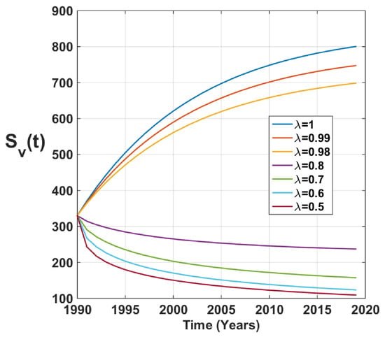
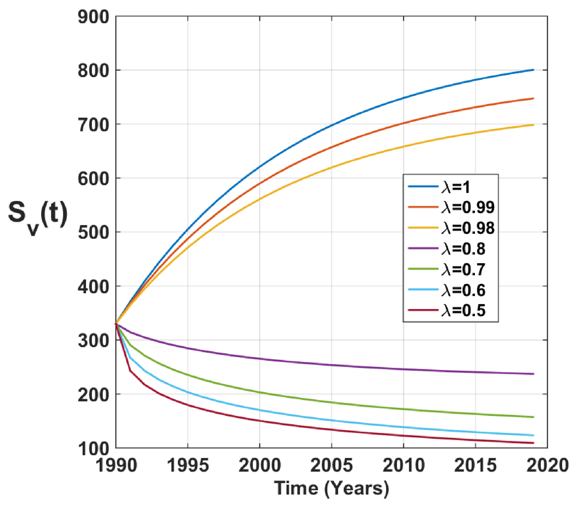
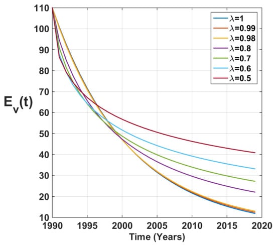
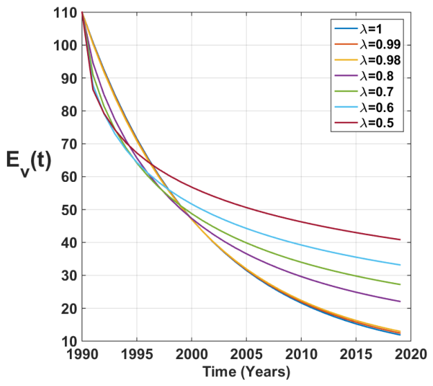
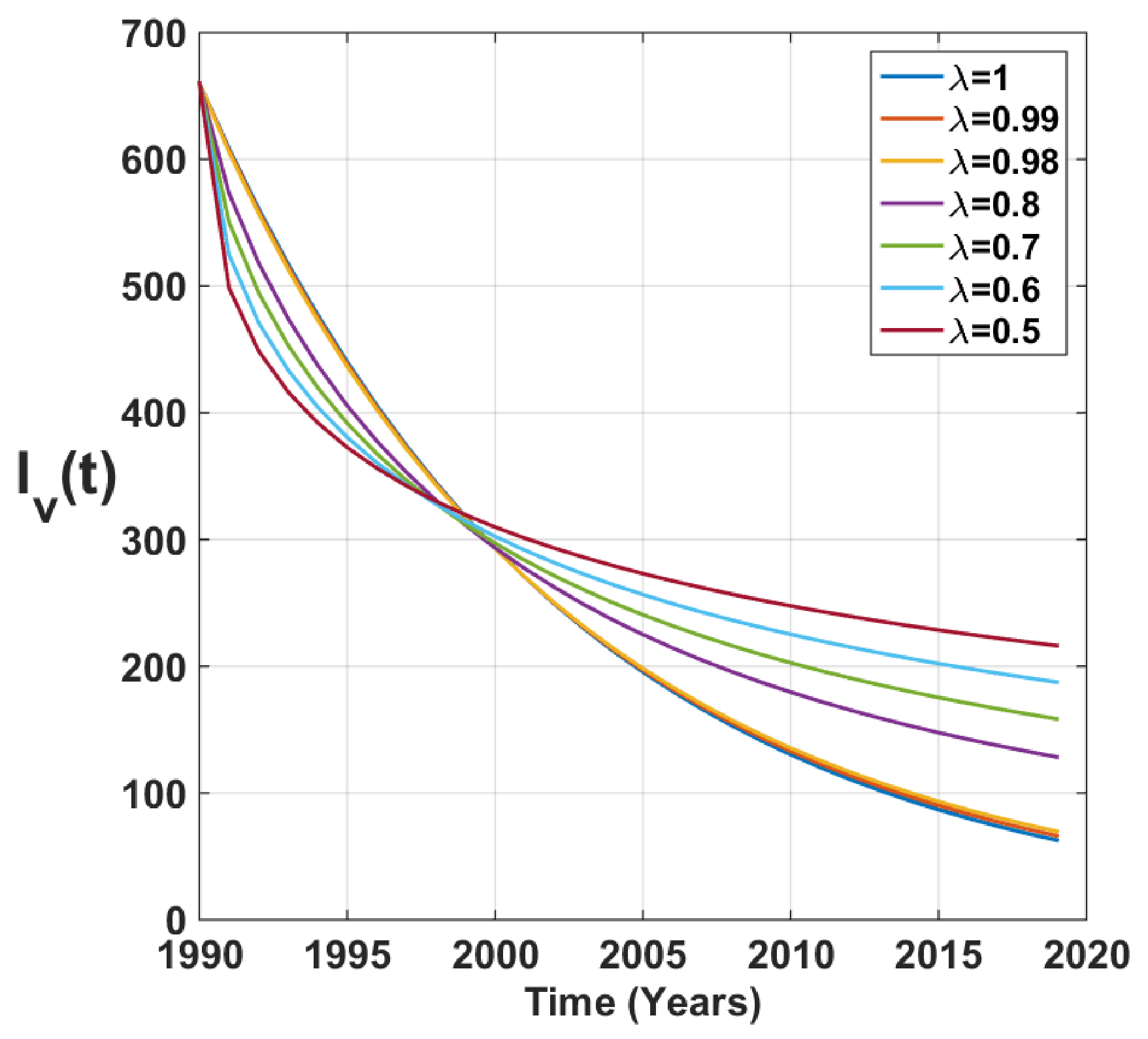
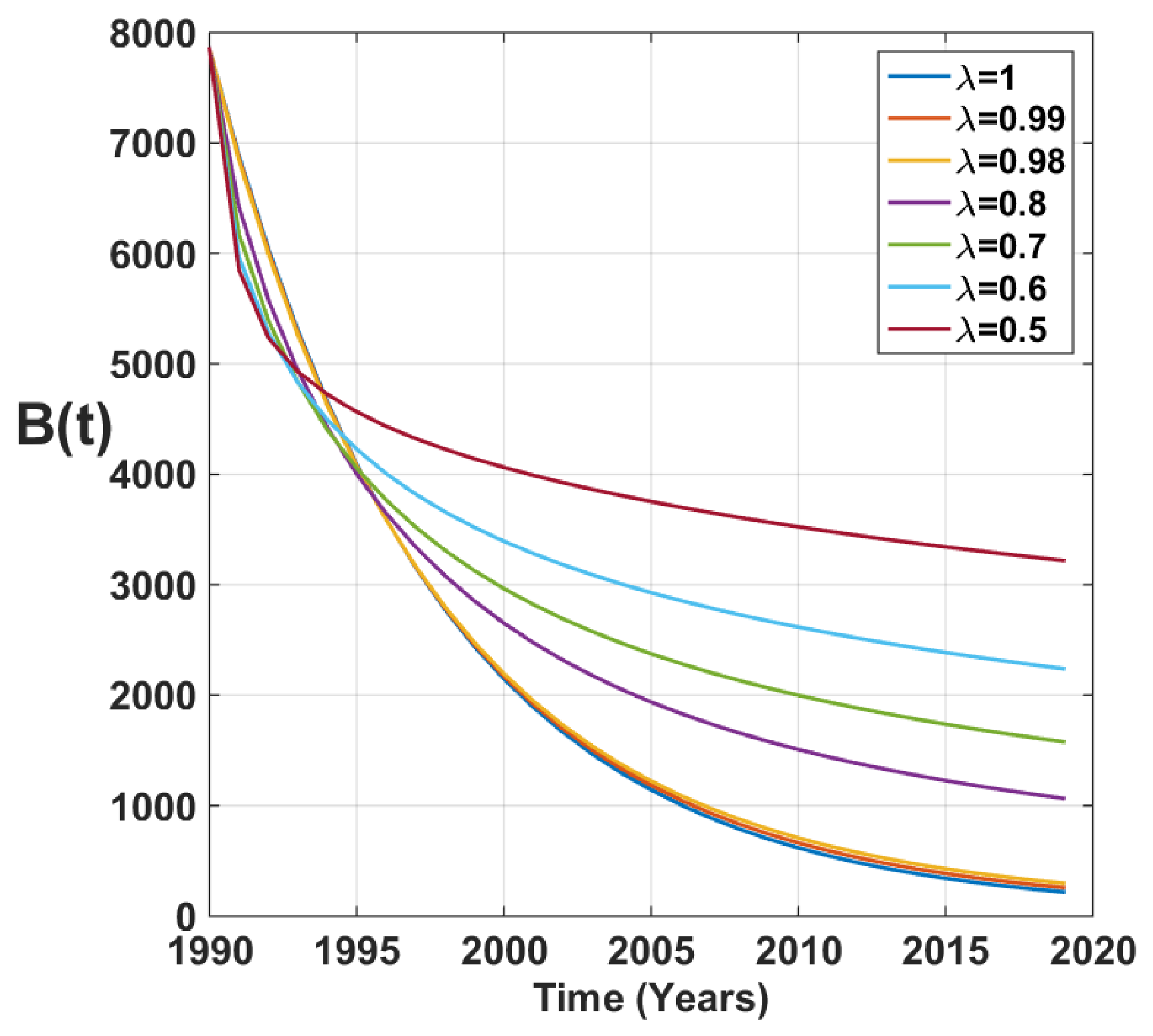
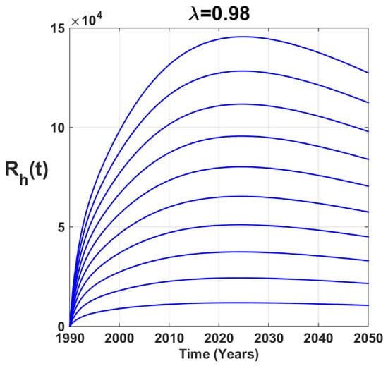
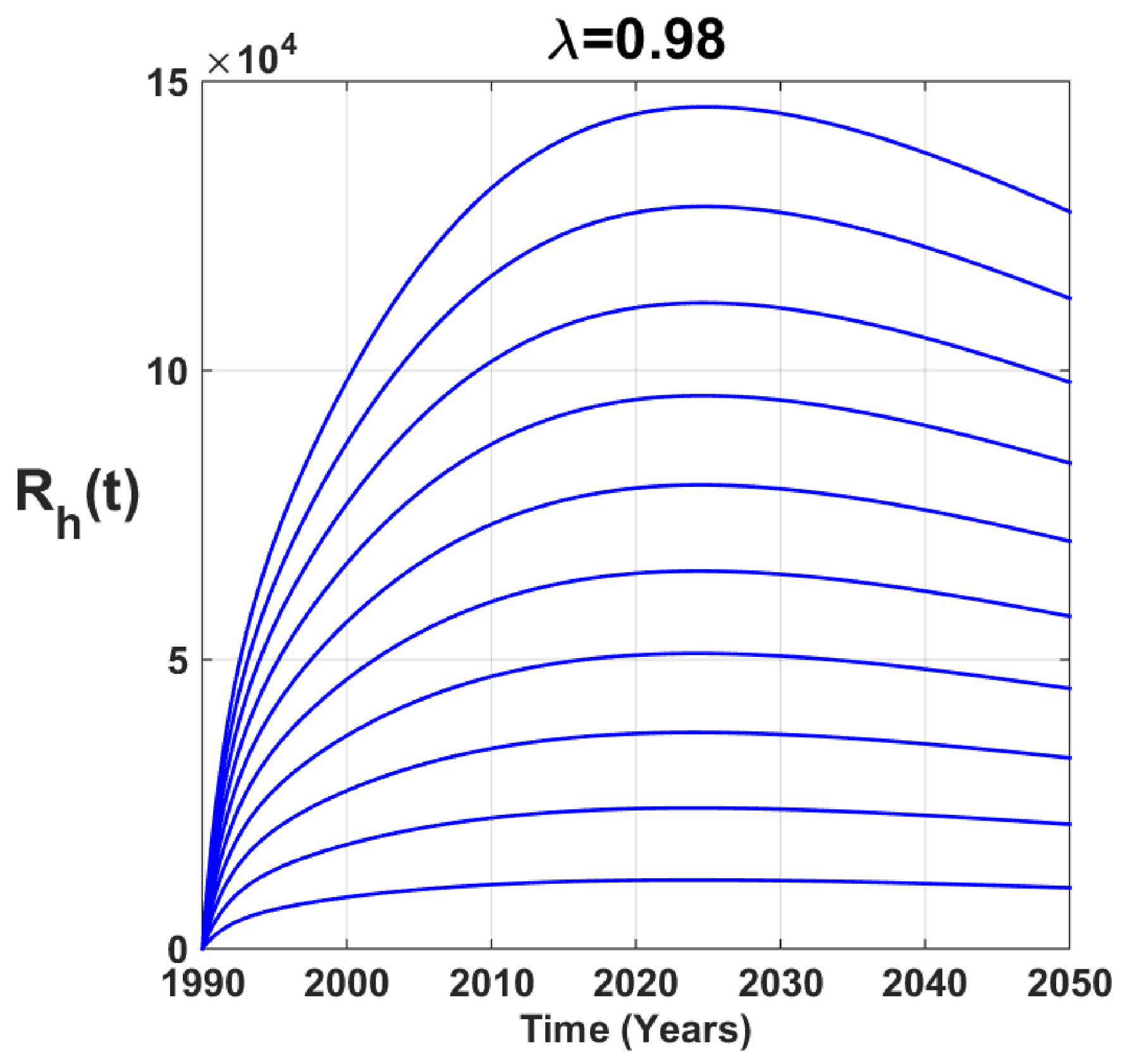
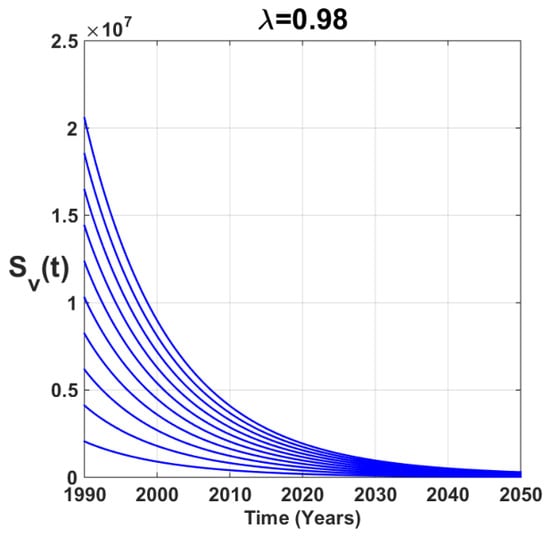
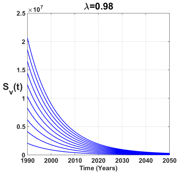
To illustrate the physical implications of the fractal model and heredity, we provide simulations of the fractional model (5) with the fractional-order parameter $\lambda$ between 1 and 0.5 (see Figure 16, Figure 17, Figure 18, Figure 19, Figure 20, Figure 21, Figure 22, Figure 23 and Figure 24). It is evident that the quantitative behavior of the model dynamics is significantly influenced by the fluctuation in $\lambda$.

Figure 16. Time series of susceptible human with values as in Table 3.

Figure 17. Time series of exposed human with values as in Table 3.

Figure 18. Time series of infectious human in the first stage of trachoma with values as in Table 3.

Figure 19. Time series of infectious human in the second stage of trachoma with values as in Table 3.

Figure 20. Time series of recovered human with values as in Table 3.

Figure 21. Time series of susceptible vectors with values as in Table 3.

Figure 22. Time series of exposed vectors with values as in Table 3.

Figure 23. Time series of infectious vectors with values as in Table 3.

Figure 24. Time series of parasite-free (B) compartments with values as in Table 3.

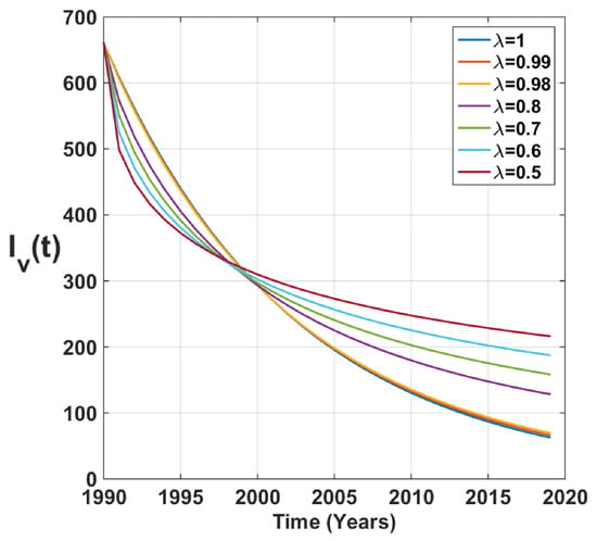
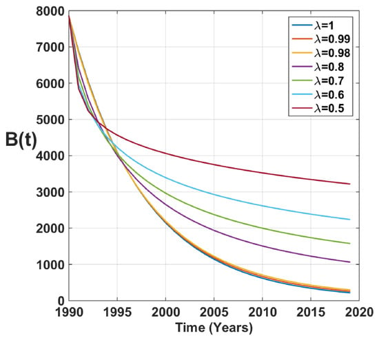
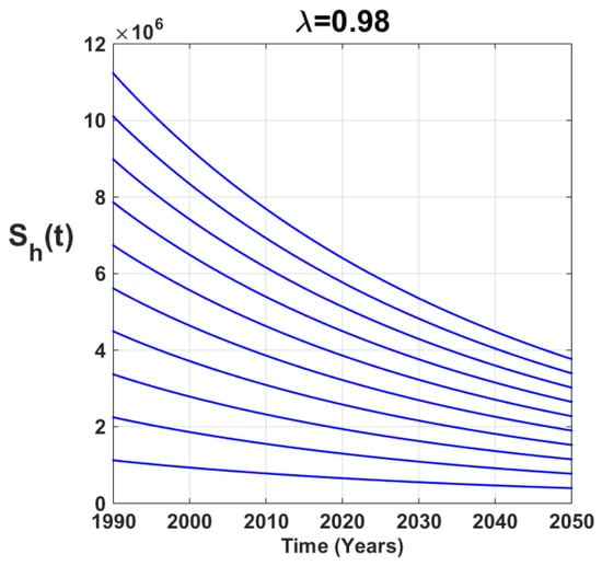
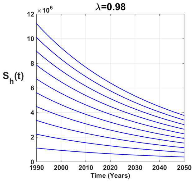
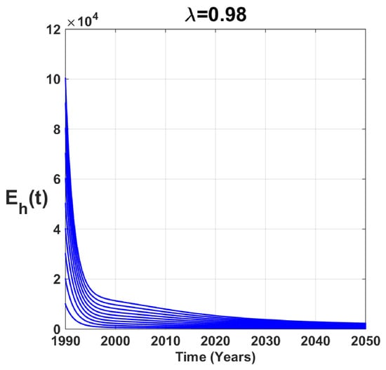
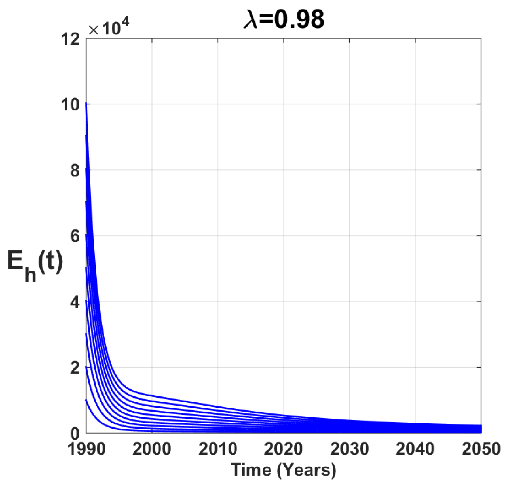
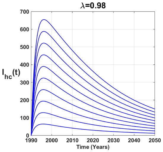
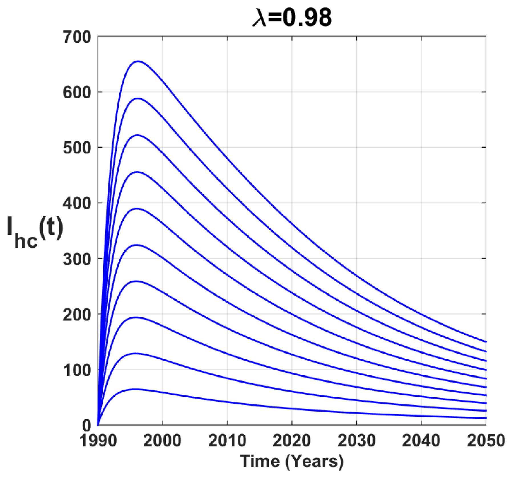
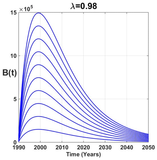
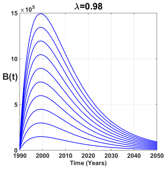
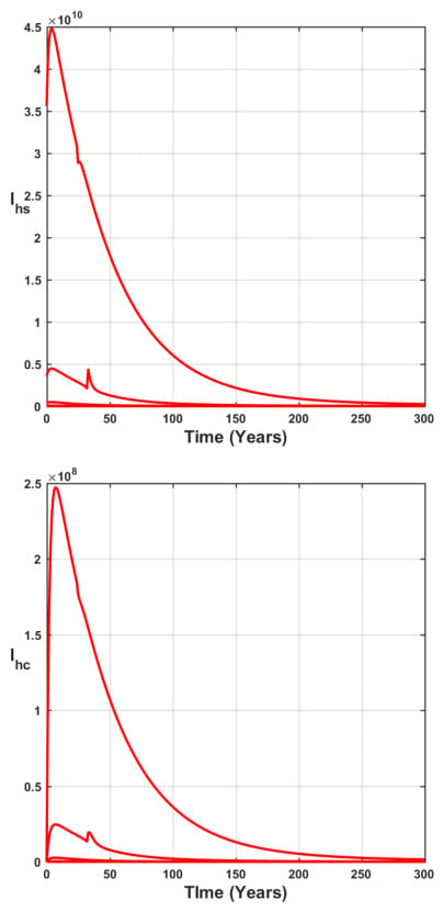
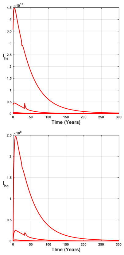
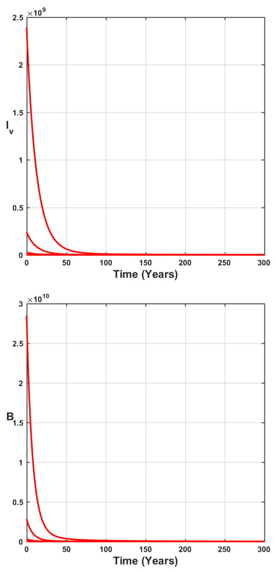
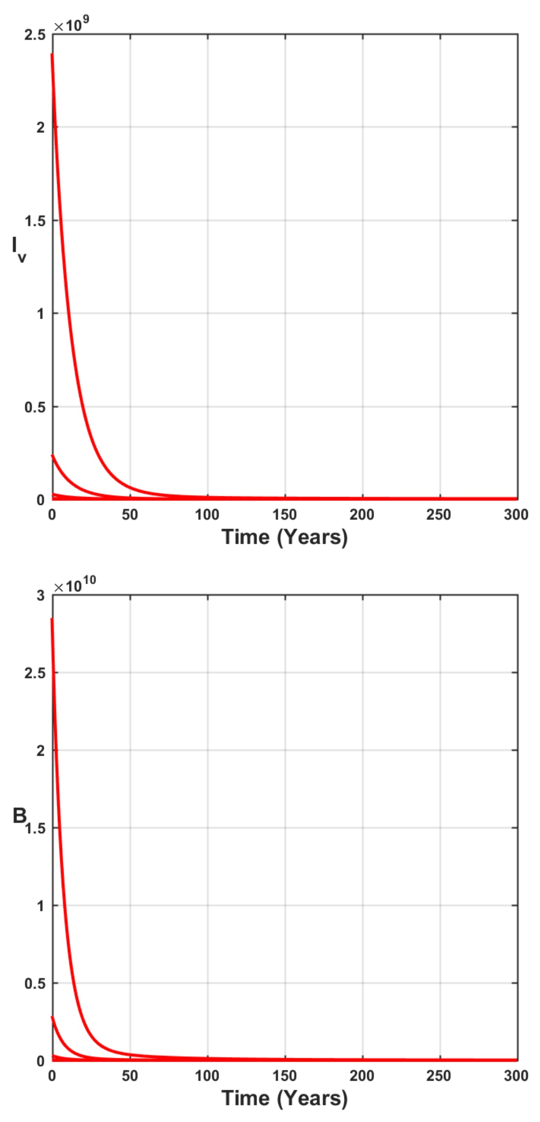
In what follows, we perform numerical simulations using $\lambda =0.98$ with different initial conditions as fractional-order. The results are displayed in Figure 25, Figure 26, Figure 27, Figure 28, Figure 29, Figure 30, Figure 31, Figure 32 and Figure 33. We observe that, for Figure 25, in the years 1995, the susceptible humans were about 1,100,000. The number of people likely to die will gradually decline to around 410,000 by 2050. For Figure 26, exposed humans numbered 10,000 in 1995. This number will gradually decrease to zero around 2050.

Figure 25. Susceptible humans for $\lambda =0.98$ with different initial conditions.

Figure 26. Time series of exposed humans for $\lambda =0.98$ with different initial conditions.

Figure 27. People with follicular inflammatory trachoma infection.

Figure 28. Humans infected with trachomatous trichiasis.

Figure 29. Recovered humans for $\lambda =0.98$ with different initial conditions.

Figure 30. Susceptible flies for $\lambda =0.98$ with different initial conditions.

Figure 31. Exposed flies for $\lambda =0.98$ with different initial conditions.

Figure 32. Infected flies for $\lambda =0.98$ with different initial conditions.

Figure 33. Pathogen with $\lambda =0.98$ and different initial conditions.

In Figure 27, we observe that, during the year 1995, there were about 10,000 humans infected with the first stage of trachoma. From 1995 to 2000, there was a slight increase in $I_{hs}$ to around 12,000. From 2005 to 2019, $I_{hs}$ gradually decreased by around 2100. In Figure 28, we observe that, in 1995, no human was infected at the second stage of the disease. From 1995 to 2000, the number of humans infected at the second stage of the disease rose steadily to around 65. And, from 2000 to 2050, they gradually decreased to 15 around 2050.

In Figure 29, in the years 1995, there were zero cured humans. But, from 1995 to 2030, there were approximately 11,900 cured humans. And from 2030 to 2050, the number of healed humans decreases and tends towards 11,100 around 2050. For Figure 30, susceptible flies increase progressively from 300 to 770 between 1995 and 2050.

The flies exposed were around 110 in 1995, as shown in Figure 31. From 1995 to 2050, they will gradually decrease, reaching 5 around 2050. Similarly, infected flies numbered around 660 in 1995, as shown in Figure 32. They decrease gradually from 1995 to 2050 and tend to about 10 around 2050.

In 1995, the bacterium was at around 7900. Bacteria decline gradually from 1995 to 2050, reaching zero around 2050 (Figure 33).

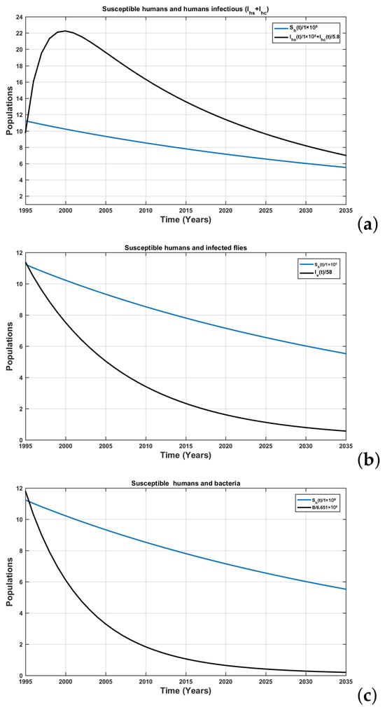
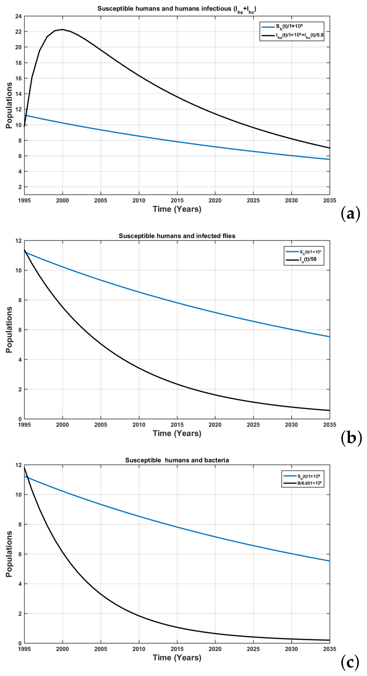
Figure 34 is obtained using the parameter values given in Table 3, for which the basic reproduction number ${\mathcal{R}}_0$ is equal to 1.169. Here we see contact between susceptible humans and infectious humans, infected flies, and bacteria. This shows the persistence of the disease.

Figure 34. Time series of: (a) susceptible humans $S_h$ and infectious humans ($I_{hs}+I_{hc}$), (b) susceptible humans and infected flies, (c) susceptible humans and bacteria.

Figure 35 and Figure 36 are obtained by using the values of the parameters given in Table 3 but this time by playing on the values of the contact rates $a_h$, $a_v$, $\nu$ for different initial conditions. To get ${\mathcal{R}}_0=0.865$, we have gradually reduced the values of the parameters $a_h$, $a_v$, and $\nu$ until $a_v=0.692341$, $a_h=0.69691$, and $\nu =0.000562$. We have demonstrated that, when control measures are put in place, the illness usually goes away over time.

Figure 35. Numerical simulation of the trachoma model (5) using Caputo when ${\mathcal{R}}_0=0.865<1$, for several initial conditions.

Figure 36. Dynamical behavior of contagious flies and environmental free pathogens using Caputo when ${\mathcal{R}}_0=0.865<1$, for several initial conditions.

Figure 34, Figure 35 and Figure 36 show the dynamic behavior of the trachoma model when ${\mathcal{R}}_0>1$ and when ${\mathcal{R}}_0<1$. The World Health Organization’s control methods significantly contribute to disease development, care quality, and trachoma eradication in Cameroon. Analyzing these methods helps identify key parameters for effective epidemic control, suggesting their importance in combating the disease.

6.3. Comparison of Deterministic Model and 5th-Order Gaussian Function

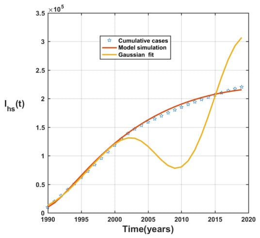
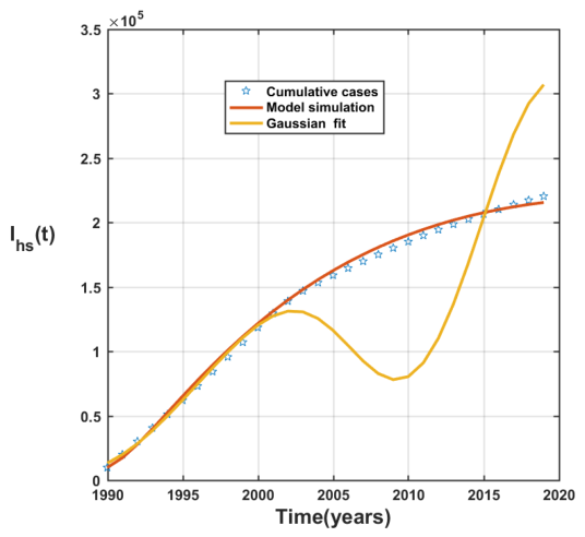
Figure 37 shows a prediction of the number of cases ($I_{hs}$) of the deterministic model and the fifth-order Gaussian function using cumulative cases. We find that the deterministic model is the one that normally follows the data, suggesting that it best approximates the real data.

Figure 37. Comparison between statistical model (yellow curve) and deterministic model (red curve) in the prediction of the number of cases ($I_{hs}$).

7. Conclusions

In summary, this work has made it possible for us to investigate a fractional derivative model of the dynamics of trachoma transmission. Using the Matlab prediction tool cftool, we first identified the statistical model that best fit the documented cases of trachoma in Cameroon between 1990 and 2019. As a result, we were able to forecast new cases over the following sixteen years (until 2035).

Next, we looked at the fractional derivative model of trachoma transmission dynamics. First, we built a fractional model that includes two population groups with two infectious stage strains and one pathogen, accounting for the dynamics of direct transmission, vector transmission, and environmental transmission. Five compartments are comprised in the first group, referred to as the human population: susceptible humans $S_h$, exposed humans $E_h$, infected humans in the first stage of the disease $I_{hs}$, infectious humans in the second stage of the disease $I_{hc}$, and cured humans $R_h$. Three compartments make up the second group, known as the fly population: susceptible flies ($S_v$), exposed flies ($E_v$), and infectious flies ($I_v$). We have used a system of nine fractional Caputo differential equations to model the dynamics of trachoma transmission across two population groups with two infectious stage strains and one pathogen. We concentrated on the model’s mathematical analysis, demonstrating the solutions’ positivity and boundedness. We have proven the existence and uniqueness of solutions by using the Banach contraction theorem. The Ulam–Hyers approach is used to determine the fractional model’s global stability. Here, we have demonstrated that the fractional model is uniformly stable in the Lyapunov sense under specific circumstances. The basic reproduction number ${\mathcal{R}}_0$ was calculated and the stability of the trachoma-free equilibrium point when ${\mathcal{R}}_0<1$ was investigated. Afterwards, we demonstrated that there is at least one endemic equilibrium point when ${\mathcal{R}}_0>1$, and prove the global stability of the unique endemic equilibrium in the special case of permanent immunity and absence of environment contamination.

We then calibrated the proposed model using data on trachoma prevalence in Cameroon and estimated the parameters using the least squares method. Given that ${\mathcal{R}}_0=1.169>1$, we conclude that trachoma is endemic in Cameroon. This is in contradiction to the fact that, with the statistical model (Gaussian function of order 5), the disease will disappear in 2035. We performed global sensitivity analysis by calculating the partial rank correlation coefficient (PRCC) between the model parameters and the basic reproduction number in order to identify key parameters in the trachoma dynamics. We found that the most important parameters are the recruitment rates of human and fly populations (${\Lambda }_h$ and ${\Lambda }_v$, respectively), the natural mortality rates of flies (${\mu }_V$), transmission rate from $S_h$ to $E_h$ ($a_h$), and transmission rate from $S_v$ to $E_v$ ($b_v$). This means that the fight against trachoma passes by the intensification of vector control mechanisms, as well as individual protections. We built the numerical scheme using the generalized Adams–Bashforth–Moulton method and analyzed its stability.

To illustrate the theoretical results, we carried out numerical simulations. We found fractional model (7) where $\lambda =0.98$ with different initial conditions better approximated the real data and thus better projected the disease dynamics in the future. Simulations were performed for fractional-order $\lambda =0.98$ with different initial conditions. We also found that the deterministic model with fractional-order derivative approximates disease behavior better than the Gaussian model.

As future work, we plan to add time-dependent control and apply the optimal control approach to determine which control strategy is better to combat the proliferation of this disease in human community.

References

- World Health Organization. Global WHO alliance for the elimination of blinding trachoma by 2020. Wkly. Epidemiol. Rec. 2012, 87, 161–168. [Google Scholar]
- Schémann, J.F. Le Trachome: Une Maladie de la Pauvreté; IRD Éditions: Marseille, France, 2013. [Google Scholar]
- Muhammad, S.M.; Hincal, E.; Mustapha, U.T.; Yusuf, A. Mathematical modeling and analysis for the transmission dynamics of blinding trachoma with effect of awareness programs. Results Phys. 2021, 28, 104683. [Google Scholar] [CrossRef] [Scilit]
- World Health Organization. Trachome. 2022. Available online: https://www.who.int/fr/news-room/fact-sheets/detail/trachoma (accessed on 31 July 2023).
- Bensaid, P.; Goldschmidt, P.; Huguet, P.; Einterz, E. Prevalence survey of blinding trachoma in the district of Kolofata-Cameroon. J. Français D’Ophtamologie 2007, 30, 528. [Google Scholar]
- Organisation Mondiale de la Santé. Intégrer les Maladies Tropicales Négligées dans L’action Pour la Santé Mondiale et le Développement: Quatrième Rapport de l’OMS sur les Maladies Tropicales Négligées; Organisation Mondiale de la Santé: Geneva, Switzerland, 2018. [Google Scholar]
- Burton, M.J.; Mabey, D.C.W. The global burden of trachoma: A review. PLoS Neglected Trop. Dis. 2009, 3, e460. [Google Scholar] [CrossRef] [Scilit] [PubMed]
- Ross, R. Some quantitative studies in epidemiology. Nature 1911, 87, 466–467. [Google Scholar] [CrossRef] [Scilit]
- Abboubakar, H.; Djouassoum, M.; Gouroudja Banbeto, S.A.; Effa, J.Y. Mathematical modelling and prediction of Tuberculosis transmission dynamics in Adamaoua region of Cameroon using fractional-order derivatives. Int. J. Model. Simul. Sci. Comput. 2025, 16, 2550060. [Google Scholar] [CrossRef] [Scilit]
- Hussain, J.; Laldinpuii, J. Vaccination strategies against SARS-CoV-2: Evaluating the impact of coverage and efficacy using a mathematical model. Model. Earth Syst. Environ. 2024, 10, 5983–6001. [Google Scholar] [CrossRef] [Scilit]
- Lawal, F.O.; Yusuf, T.T.; Abidemi, A.; Olotu, O. A non-linear mathematical model for typhoid fever transmission dynamics with medically hygienic compartment. Model. Earth Syst. Environ. 2024, 10, 6213–6232. [Google Scholar] [CrossRef] [Scilit]
- Ramzan, S.; Rashid, S.; Shah, M.A.; Elagan, S.K. Exploring the dynamical bifurcation and stability analysis of Nipah virus; novel perspectives utilizing fractional calculus. Model. Earth Syst. Environ. 2024, 10, 5427–5448. [Google Scholar] [CrossRef] [Scilit]
- Olopade, I.; Ajao, S.; Akinwumi, T.; Adeniran, G.; Aderenle, R.; Adesanya, A. Mathematical modelling of the impacts of syphilis multi-stage treatments. Model. Earth Syst. Environ. 2024, 10, 5489–5502. [Google Scholar] [CrossRef] [Scilit]
- Fandio, R.; Abboubakar, H.; Banbeto, S.A.G.; Fouda, H.P.E. Mathematical modeling of the Cholera epidemic in Cameroon: From classical-order derivative to fractional-order derivative. MJ Math. Comput. Sci. 2025, 1, 1–32. [Google Scholar] [CrossRef] [Scilit]
- Guidzavaï, A.K.; Yangla, J.; Abboubakar, H.; Kaakréo, G.; Fandio, R.; Damakoa, I. Mathematical modeling of SARS-CoV-2 (COVID-19) pandemic in Cameroon accounting the role of boosted immune systems. MJ Math. Comput. Sci. 2026, 2, 1–32. [Google Scholar]
- Atsbha, S.G. A review of the prevalence of trachoma, its control program and challenges in Ethiopia. Int. J. Drug Regul. Aff. 2023, 11, 54–60. [Google Scholar] [CrossRef] [Scilit]
- Solomon, A.W.; Pavluck, A.L.; Courtright, P.; Aboe, A.; Adamu, L.; Alemayehu, W.; Alemu, M.; Alexander, N.D.E.; Kello, A.B.; Bero, B.; et al. The Global Trachoma Mapping Project: Methodology of a 34-country population-based study. Ophthalmic Epidemiol. 2015, 22, 214–225. [Google Scholar] [CrossRef] [Scilit]
- Gambhir, M.; Basáñez, M.G.; Burton, M.J.; Solomon, A.W.; Bailey, R.L.; Holland, M.J.; Blake, I.M.; Donnelly, C.A.; Jabr, I.; Mabey, D.C.; et al. The development of an age-structured model for trachoma transmission dynamics, pathogenesis and control. PLoS Neglected Trop. Dis. 2009, 3, e462. [Google Scholar] [CrossRef] [Scilit]
- Pinsent, A.; Hollingsworth, T.D. Optimising sampling regimes and data collection to inform surveillance for trachoma control. PLoS Neglected Trop. Dis. 2018, 12, e0006531. [Google Scholar] [CrossRef] [Scilit]
- Hu, V.H.; Harding-Esch, E.M.; Burton, M.J.; Bailey, R.L.; Kadimpeul, J.; Mabey, D.C.W. Epidemiology and control of trachoma: Systematic review. Trop. Med. Int. Health 2010, 15, 673–691. [Google Scholar] [CrossRef] [Scilit] [PubMed]
- Ndisabiye, D.; Waters, E.; Gore, R.; Sidhu, H. Do poor environmental conditions drive trachoma transmission in Burundi? A mathematical modelling study. ANZIAM J. 2021, 63, 434–447. [Google Scholar]
- Chen, Y.Q.; Petras, I.; Xue, D. Fractional order control—A tutorial. In Proceedings of the 2009 American Control Conference; IEEE: New York, NY, USA, 2009; pp. 1397–1411. [Google Scholar]
- Nisar, K.S.; Farman, M.; Abdel-Aty, M.; Ravichandran, C. A review of fractional order epidemic models for life sciences problems: Past, present and future. Alex. Eng. J. 2024, 95, 283–305. [Google Scholar] [CrossRef] [Scilit]
- Nabi, K.N.; Abboubakar, H.; Kumar, P. Forecasting of COVID-19 pandemic: From integer derivatives to fractional derivatives. Chaos Solitons Fractals 2020, 141, 110283. [Google Scholar] [CrossRef] [Scilit]
- Atangana, A.; Alqahtani, R.T. Numerical approximation of the space-time Caputo-Fabrizio fractional derivative and application to groundwater pollution equation. Adv. Differ. Equ. 2016, 2016, 156. [Google Scholar] [CrossRef] [Scilit]
- Atangana, A.; Vermeulen, P.D. Analytical solutions of a space-time fractional derivative of groundwater flow equation. Abstr. Appl. Anal. 2014, 2014, 381753. [Google Scholar] [CrossRef] [Scilit]
- Atangana, A. Application of fractional calculus to epidemiology. Fract. Dyn. 2015, 2015, 174–190. [Google Scholar]
- Atangana, A.; Araz, S.İ. Fractional Stochastic Differential Equations: Applications to COVID-19 Modeling; Springer Nature: Berlin/Heidelberg, Germany, 2022. [Google Scholar]
- Thirthar, A.A.; Abboubakar, H.; Khan, A.; Abdeljawad, T. Mathematical modeling of the COVID-19 epidemic with fear impact. AIMS Math. 2023, 8, 6447–6465. [Google Scholar] [CrossRef] [Scilit]
- Khan, T.; Ullah, R.; Zaman, G.; Alzabut, J. A mathematical model for the dynamics of SARS-CoV-2 virus using the Caputo-Fabrizio operator. Math. Biosci. Eng. 2021, 18, 6095–6116. [Google Scholar] [CrossRef] [Scilit]
- Ahmad, S.; ur Rahman, M.; Arfan, M. On the analysis of semi-analytical solutions of Hepatitis B epidemic model under the Caputo-Fabrizio operator. Chaos Solitons Fractals 2021, 146, 110892. [Google Scholar] [CrossRef] [Scilit]
- Ray, S.S.; Atangana, A.; Noutchie, S.C.O.; Kurulay, M.; Bildik, N.; Kilicman, A. Fractional calculus and its applications in applied mathematics and other sciences. Math. Probl. Eng. 2014, 2014, 849395. [Google Scholar] [CrossRef] [Scilit]
- Qureshi, S.; Yusuf, A. Modeling chickenpox disease with fractional derivatives: From caputo to atangana-baleanu. Chaos Solitons Fractals 2019, 122, 111–118. [Google Scholar] [CrossRef] [Scilit]
- Our World in Data Team. Trachoma Prevalence Rate, 2019. 1990–2019. Available online: https://ourworldindata.org/grapher/trachoma-prevalence-age-standardized-ihme (accessed on 18 August 2023).
- Noa Noatina, B.; Kagmeni, G.; Mengouo, M.N.; Moungui, H.C.; Tarini, A.; Zhang, Y.; Bella, A.L.F. Prevalence of trachoma in the Far North region of Cameroon: Results of a survey in 27 Health Districts. PLoS Neglected Trop. Dis. 2013, 7, e2240. [Google Scholar] [CrossRef] [Scilit]
- Podlubny, I. Fractional Differential Equations: An Introduction to Fractional Derivatives, Fractional Differential Equations, to Methods of Their Solution and Some of Their Applications; Elsevier: Amsterdam, The Netherlands, 1998. [Google Scholar]
- Sallet, G. CIMPA Lecture Notes on Mathematical Epidemiology (March 2018); CIMPA: Nice, France, 2018. [Google Scholar]
- Dorrego, G.A.; Cerutti, R.A. The k-Mittag-Leffler function. Int. J. Contemp. Math. Sci. 2012, 7, 705–716. [Google Scholar]
- Lin, W. Global existence theory and chaos control of fractional differential equations. J. Math. Anal. Appl. 2007, 332, 709–726. [Google Scholar] [CrossRef] [Scilit]
- El-Sayed, A.M. On the existence and stability of positive solution for a nonlinear fractional-order differential equation and some applications. Alex. J. Math. 2010, 1, 1–10. [Google Scholar]
- Jung, S.M. Hyers-Ulam-Rassias Stability of Functional Equations in Nonlinear Analysis; Springer Science & Business Media: Berlin/Heidelberg, Germany, 2011; Volume 48. [Google Scholar]
- Van den Driessche, P.; Watmough, J. Reproduction numbers and sub-threshold endemic equilibria for compartmental models of disease transmission. Math. Biosci. 2002, 180, 29–48. [Google Scholar] [CrossRef] [Scilit]
- Shuai, Z.; van den Driessche, P. Global stability of infectious disease models using Lyapunov functions. SIAM J. Appl. Math. 2013, 73, 1513–1532. [Google Scholar] [CrossRef] [Scilit]
- LaSalle, J.P. Stability theory and invariance principles. In Dynamical Systems; Elsevier: Amsterdam, The Netherlands, 1976; pp. 211–222. [Google Scholar]
- Maxima Development Team. Maxima, version 2009; Maxima AI: San Mateo, CA, USA, 2019. [Google Scholar]
- Rodríguez Galván, J.R. Maxima con wxMaxima: Software Libre en el Aula de Matemáticas; Universidad de Cádiz: Cádiz, Spain, 2017. [Google Scholar]
- Santos, B. Introduçao ao Software MAXIMA; Centro de Matemática da Universidade do Porto: Porto, Portugal, 2009. [Google Scholar]
- Curtiss, D.R. Recent extentions of descartes’ rule of signs. Ann. Math. 1918, 19, 251–278. [Google Scholar] [CrossRef] [Scilit]
- Abboubakar, H.; Kouchéré Guidzavaï, A.; Yangla, J.; Damakoa, I.; Mouangue, R. Mathematical modeling and projections of a vector-borne disease with optimal control strategies: A case study of the Chikungunya in Chad. Chaos Solitons Fractals 2021, 150, 111197. [Google Scholar] [CrossRef] [Scilit]
- Boukhouima, A.; Hattaf, K.; Lotfi, E.M.; Mahrouf, M.; Torres, D.F.; Yousfi, N. Lyapunov functions for fractional-order systems in biology: Methods and applications. Chaos Solitons Fractals 2020, 140, 110224. [Google Scholar] [CrossRef] [Scilit]
- Lahrouz, A.; Hajjami, R.; El Jarroudi, M.; Settati, A.; Erriani, M. Invariant set theorems for non-autonomous time-fractional systems. Int. J. Dyn. Control 2023, 12, 2280–2294. [Google Scholar] [CrossRef] [Scilit]
- Björck, Å. Numerical Methods for Least Squares Problems; SIAM: Bangkok, Thailand, 2024. [Google Scholar]
- Atangana, A. Mathematical model of survival of fractional calculus, critics and their impact: How singular is our world? Adv. Differ. Equ. 2021, 2021, 403. [Google Scholar] [CrossRef] [Scilit]
- Fandio, R.; Abboubakar, H.; Fouda, H.P.E.; Kumar, A.; Nisar, K.S. Mathematical modelling and projection of Buruli ulcer transmission dynamics using classical and fractional derivatives: A case study of Cameroon. Partial Differ. Equ. Appl. Math. 2023, 8, 100589. [Google Scholar] [CrossRef] [Scilit]
- Stein, M. Large sample properties of simulations using Latin hypercube sampling. Technometrics 1987, 29, 143–151. [Google Scholar] [CrossRef]
- Marino, S.; Hogue, I.B.; Ray, C.J.; Kirschner, D.E. A methodology for performing global uncertainty and sensitivity analysis in systems biology. J. Theor. Biol. 2008, 254, 178–196. [Google Scholar] [CrossRef] [Scilit] [PubMed]
- Wu, J.; Dhingra, R.; Gambhir, M.; Remais, J.V. Sensitivity analysis of infectious disease models: Methods, advances and their application. J. R. Soc. Interface 2013, 10, 20121018. [Google Scholar] [CrossRef] [Scilit] [PubMed]
- Abboubakar, H.; Claude Kamgang, J.; Tieudjo, D. Backward bifurcation and control in transmission dynamics of arboviral diseases. Math. Biosci. 2016, 278, 100–129. [Google Scholar] [CrossRef] [Scilit]
- Hajaj, R.; Odibat, Z. Numerical solutions of fractional epidemic models with generalized Caputo-type derivatives. Phys. Scr. 2023, 98, 045206. [Google Scholar] [CrossRef] [Scilit]
- Mahatekar, Y.M.; Kumar, P. A novel numerical method to solve fractional ordinary differential equations with proportional Caputo derivatives. Phys. Scr. 2024, 99, 105261. [Google Scholar] [CrossRef] [Scilit]
- Odibat, Z. Numerical simulation of fractional-order Duffing system with extended Mittag-Leffler derivatives. Phys. Scr. 2024, 99, 075217. [Google Scholar] [CrossRef] [Scilit]
- Odibat, Z.; Erturk, V.S.; Kumar, P.; Govindaraj, V. Dynamics of generalized Caputo type delay fractional differential equations using a modified Predictor-Corrector scheme. Phys. Scr. 2021, 96, 125213. [Google Scholar] [CrossRef] [Scilit]
- Yepez-Martinez, H.; Gómez-Aguilar, J.F.; Inc, M. New modified Atangana-Baleanu fractional derivative applied to solve nonlinear fractional dierential equations. Phys. Scr. 2023, 98, 035202. [Google Scholar] [CrossRef] [Scilit]
- Odibat, Z. On a fractional derivative operator with a singular kernel: Definition, properties and numerical simulation. Phys. Scr. 2024, 99, 075278. [Google Scholar] [CrossRef] [Scilit]
- Li, C.; Tao, C. On the fractional Adams method. Comput. Math. Appl. 2009, 58, 1573–1588. [Google Scholar] [CrossRef] [Scilit]
- Diethelm, K.; Ford, N.J. Analysis of fractional differential equations. J. Math. Anal. Appl. 2002, 265, 229–248. [Google Scholar] [CrossRef] [Scilit]
- Diethelm, K. An algorithm for the numerical solution of differential equations of fractional order. Electron. Trans. Numer. Anal. 1997, 5, 1–6. [Google Scholar]
- Li, C.; Zeng, F. The finite difference methods for fractional ordinary differential equations. Numer. Funct. Anal. Optim. 2013, 34, 149–179. [Google Scholar] [CrossRef] [Scilit]
- Abboubakar, H.; Kom Regonne, R.; Sooppy Nisar, K. Fractional dynamics of typhoid fever transmission models with mass vaccination perspectives. Fractal Fract. 2021, 5, 149. [Google Scholar] [CrossRef] [Scilit]
- Liu, F.; Porco, T.C.; Ray, K.J.; Bailey, R.L.; Mkocha, H.; Muñoz, B.; Quinn, T.C.; Lietman, T.M.; West, S.K. Assessment of transmission in trachoma programs over time suggests no short-term loss of immunity. PLoS Neglected Trop. Dis. 2013, 7, e2303. [Google Scholar] [CrossRef] [Scilit]
- Emerson, P.M.; Bailey, R.L.; Mahdi, O.S.; Walraven, G.E.; Lindsay, S.W. Transmission ecology of the fly Musca sorbens, a putative vector of trachoma. Trans. R. Soc. Trop. Med. Hyg. 2000, 94, 28–32. [Google Scholar] [CrossRef] [Scilit]
Disclaimer/Publisher’s Note: The statements, opinions and data contained in all publications are solely those of the individual author(s) and contributor(s) and not of MDPI and/or the editor(s). MDPI and/or the editor(s) disclaim responsibility for any injury to people or property resulting from any ideas, methods, instructions or products referred to in the content. |
© 2026 by the authors. Licensee MDPI, Basel, Switzerland. This article is an open access article distributed under the terms and conditions of the Creative Commons Attribution (CC BY) license.