Fractal Modeling and Coordinated Evolution of Railway Networks in China’s Urban Systems: A Dual Perspective of Spatial Distribution and Temporal Accessibility

Abstract

Railways constitute a core component of China’s national comprehensive transportation network, and their spatial organization and temporal accessibility jointly shape transport integration and system efficiency. Identifying their evolution from the dual perspectives of spatial expansion and time compression is therefore of both theoretical and practical significance. Drawing on fractal theory, this study examines the structural characteristics, evolutionary trends, and driving factors of railway networks in China’s five major urban systems from 2014 to 2024 from a “space–time” dual perspective. The results show that railway networks exhibit a staged pattern of “spatial filling preceding temporal correlation”, with a lag of approximately 1–8 years—about 1 year in the Guangdong–Hong Kong–Macao Greater Bay Area (GBA), 5 years in the Middle Yangtze River (MYR) region and Beijing–Tianjin–Hebei (BTH), and up to 8 years in the Chengdu–Chongqing (CC) region. In addition, clear regional differences are observed: the Yangtze River Delta (YRD) is polycentric, with the greatest potential, projected to continue rapid spatial growth until 2027 and to remain in a fast-growth phase of temporal correlation; GBA is highly coordinated; BTH is developed but characterized by dual-core agglomeration; CC grows rapidly with lagging functionality; and MYR is corridor-dependent with limited potential. These findings indicate that network functionality does not emerge synchronously with infrastructure expansion, but depends on subsequent improvements in operational organization and service capacity. Compared with single-scale-based indicators, the “spatial distribution–temporal correlation” framework more effectively captures network performance and provides quantitative support for transport optimization and coordinated regional development.

1. Introduction

Transportation networks are typical complex systems characterized by complexity in both spatial configuration and operational management. Their evolution can therefore be characterized within a unified “spatial structure–temporal efficiency” framework [1]. Spatial structure refers to morphological attributes such as route length and node density, which form the material basis of transport capacity and spatial coverage. Temporal efficiency, by contrast, concerns travel time, service frequency, and the resulting improvements in spatiotemporal accessibility, which directly influence travel behavior and intercity interactions. These correspond to the “space of places” and the “space of flows” in geography [2]. Enhanced accessibility effectively “compresses” geographic distance in socio-economic terms, reducing spatial barriers and producing the time–space compression effect [3]. Integrating spatial expansion and time–space compression enables more accurate identification of differentiated pathways and mechanisms of network development, providing a basis for urban system typology and transport–spatial policy design.

Fractal theory offers a powerful framework for analyzing self-organization and scaling properties in complex systems and is well suited to transportation networks. A variety of fractal algorithms have been developed, among which box-counting and radius-based methods are the most commonly used in transportation network studies. Different fractal algorithms capture complementary aspects. For example, box-counting methods emphasize spatial distribution and space-filling characteristics [4,5,6,7,8,9], whereas radius-based methods focus on correlational structures and clustering, supporting analysis of temporal correlation and interaction intensity [10,11,12,13,14]. Combining these methods enables a more comprehensive characterization of system complexity.

Existing studies have applied various fractal methods to examine the spatial configuration and service operation of transportation networks (

Table 1. Applications of Fractal Methods in Transportation Network Studies.

Category	Physical Network	Service Network
Study object	Spatial distribution of infrastructure	A weighted graph, where edge weights denote train frequency, passenger flow, or travel time.
Corresponding geographic space	Space of places	Space of flows
Data sources	Map data (e.g., OSM)	Timetable data, travel time data, traffic flow data
Monofractal methods	Box [4,5] and radius [10,11] methods to measure spatial filling and its relationship with urban expansion. Head/tail breaks for hierarchical structure identification [15,16].	Radial dimension to characterize aggregation patterns [14,17]. Fractal dimension defined in flow space to evaluate job–housing flows [9].
Multifractal methods	Box [6,7] and sandbox [12,13] methods to capture spatial heterogeneity.	Box method to characterize heterogeneity in travel time [8].
Dual-perspective studies	Box and radius methods, along with head/tail breaks, are used to measure geometric, topological, and hierarchical structures [18], but comparative analysis and the exploration of evolutionary characteristics remain insufficient.

). Physical network studies, typically based on map data, use box [4,5,6,7], radius [10,11], sandbox [12,13] and head/tail breaks methods [15,16] to characterize spatial filling, hierarchy, and heterogeneity. In contrast, service network studies rely on timetable and travel-time data to analyze accessibility and flow patterns, mainly using box [8,9] and radius-based [14,17] methods. However, despite the use of both monofractal and multifractal approaches, most studies remain limited to a single method or dimension, lacking an integrated analysis of spatial–temporal linkages and a unified analytical framework. Even when multiple methods are combined [18], analyses are largely descriptive, with limited quantitative comparison and insufficient exploration of evolutionary dynamics across different aspects of transportation networks.

In summary, existing fractal studies tend to focus on single-dimensional or static characteristics of transportation networks, and a unified and comparable framework integrating spatial distribution and temporal correlation remains lacking. The scientific objective of this study is to address this gap by developing a fractal-based analytical framework to systematically examine the spatial distribution, temporal correlation, and evolutionary dynamics of transportation networks, as well as to identify the key mechanisms underlying time–space compression. The empirical focus and practical purpose of this study are to apply this framework to railway networks, which serve as the backbone of intercity connectivity. Using the five major urban agglomerations in China as case studies, the research aims to reveal differentiated evolutionary patterns and to provide scientific support for optimizing network layout, improving operational efficiency, and informing targeted transport and spatial development policies.

2. Materials and Methods

2.1. Fractal Model

Transportation network optimization is a key research topic in the field of transportation planning. As a prototypical form of naturally optimized structure, fractals occupy space with maximal efficiency [19]. Therefore, fractal theory provides a theoretical framework for explaining structural or functional problems in urban transportation systems, offering a scientific basis for evaluating the rationality of transportation network structures and the degree of optimization.

The core of fractal theory lies in the concept of scaling relationships. Although the measured value of a fractal object varies with the measurement scale, the two maintain a stable power-law (scaling) relationship within a certain scale range [20,21]. Fractal geometry replaces a single measurement outcome with an explicit measurement process, extracting scaling exponents (related to fractal dimensions) from the scale-measure power-law relationship to quantify system complexity and the degree of space filling [22,23]. For example, by measuring a transportation network at different spatial scales r, a corresponding metric L(r) can be obtained for each scale. If the relationship between the scale and the metric follows a scaling-invariant law, as expressed by

$$L(\lambda r)\propto {\lambda }^{a}L(r),$$

(1)

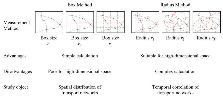
then the transportation network of an urban system can be considered scale-invariant. Here, λ represents the scale ratio, and a denotes the scaling exponent, which is related to the fractal dimension. Therefore, the fractal dimension can be derived from Equation (1), and it characterizes different structural features of transportation networks depending on the measurement method. Generally, fractal algorithms can be classified into two categories according to measurement schemes: fixed-size algorithms (FSA) and fixed-mass algorithms (FMA) [24,25,26]. Fractal studies predominantly adopt FSA, including the box-counting and radius-based methods [27], as well as time-series-based approaches such as the wavelet transform method [28] and detrended fluctuation analysis [29]. Among these, the box-counting and radius-based methods are the most widely used in transportation network analysis [4,6,9,14] (Figure 1).

The box-counting method, the most widely applied technique for estimating fractal dimensions, originates from a basic geometric principle [27]: an object is covered with a series of boxes, and as the box size decreases, the total area of occupied boxes approaches the actual area of the object. However, in the case of fractal phenomena, the measurement result inherently depends on the scale. Therefore, rather than emphasizing the absolute measurement itself, attention should be directed toward the scaling relationship revealed through the measurement process. For instance, by counting the number of non-empty boxes S(r) at different box sizes r, the following relationship can be derived:

$$S(r)\propto r^{-D_b},$$

(2)

where D_b represents the capacity dimension, with a theoretical range of 0–2 in geographical space, reflecting the degree of spatial filling. Among various box-counting approaches, the functional box method is commonly used [30,31]. In this method, the study area is first enclosed by its minimum bounding rectangle, which provides a consistent spatial extent for measurement and helps improve estimation accuracy [32]. The rectangle is then recursively subdivided into smaller grids (as illustrated in Figure 1). At each step, it is divided into 4, 16, … equal cells, with the box size defined as the corresponding scale r.

The radius method, in contrast, takes a point i on the fractal as the center and draws a circle of radius r [33]. It then calculates the proportion C_i(r) of particles falling within the circle relative to the total number of particles N:

$$C_i(r)={\displaystyle \frac{1}{N}}{\displaystyle \sum _j^N\theta (r-d_{ij})},$$

(3)

where d_ij denotes the distance between points i and j, and θ is the Heaviside function defined as:

$$\theta (x)=\left\{\begin{array}{c}1,x\ge 0\\ 0,x<0\end{array}\right..$$

(4)

This leads to the following scaling relationship:

$$C_i(r)\propto r^{D_{\alpha }},$$

(5)

where D_α is the radial dimension, describing the local spatial association of a point within the urban system. In geographical space, its theoretical range is 0–3, with the critical value equal to the Euclidean dimension of the embedding space (i.e., 2) [34]. The radial dimension of a regional central city reflects the relationship between the center and its hinterland as well as its concentration distribution tendency. When D_α = 2, the urban density remains constant, indicating a uniform Euclidean distribution around the center. When D_α < 2, density decreases with increasing distance from the center, showing centripetal clustering—and the smaller D_α, the stronger the centralization. Conversely, when D_α > 2, density increases with distance, showing centrifugal dispersion—and the larger the D_α, the stronger the decentralization. Considering all points on the fractal, the correlation function C(r) can be expressed as:

$$C(r)={\displaystyle \frac{1}{N}}{\displaystyle \sum _i^N{C}_i(r)}={\displaystyle \frac{1}{N^2}}{\displaystyle \sum _i^N{\displaystyle \sum _j^N\theta (r-d_{ij})}}\propto r^{D_c},$$

(6)

where D_c denotes the correlation dimension, reflecting the global spatial association. Its theoretical range in geographical space is 0–2.

Both the box-counting and radius methods have their advantages and limitations, but they can be unified under a multifractal framework [33,35,36]. The box-counting method is computationally simple but unsuitable for high-dimensional spaces, whereas the radius method is more applicable to high-dimensional data but computationally intensive. Therefore, this study employs the box method (specifically, the functional box approach) to analyze the spatial distribution of transportation networks and the radius method to analyze their temporal correlation (Figure 1).

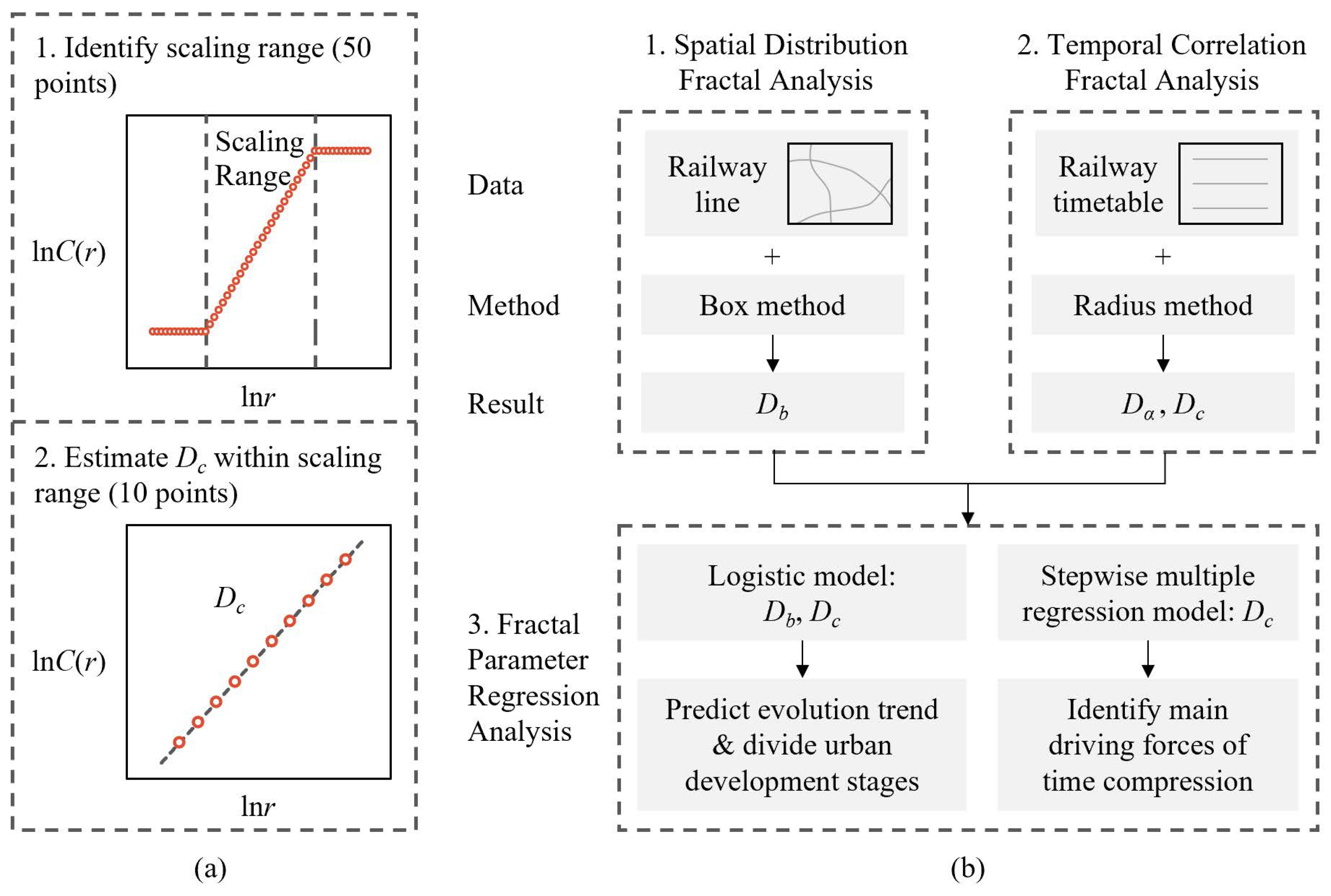
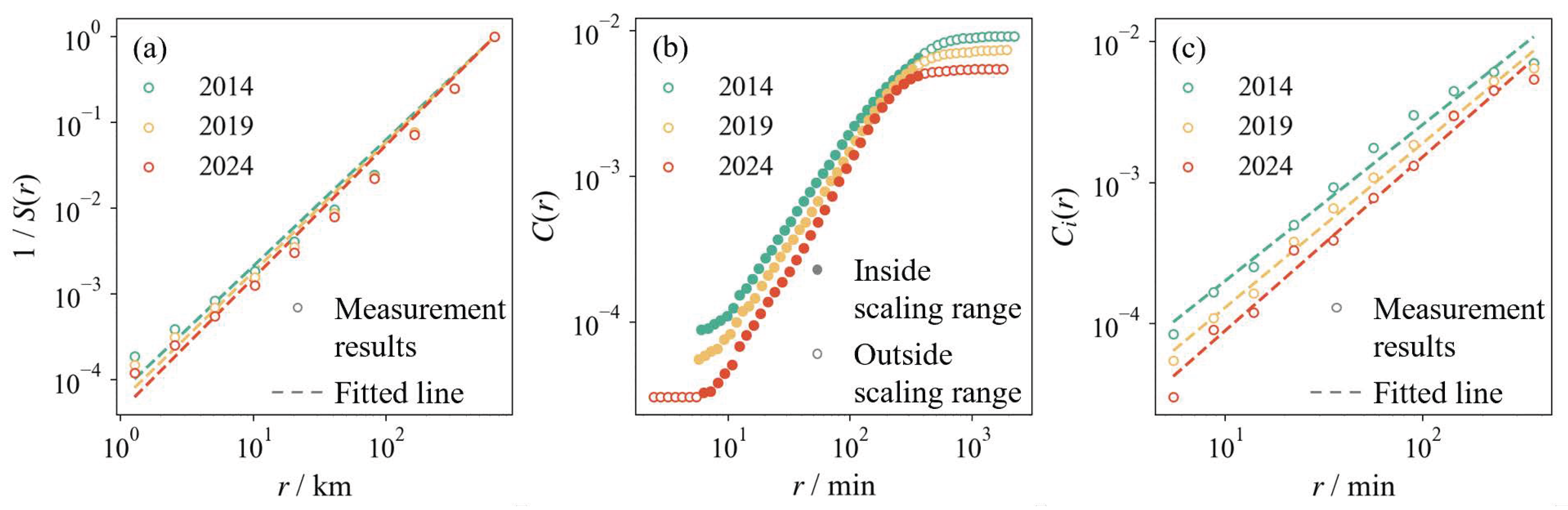
In reality, perfect fractals do not exist, and discrepancies arise between fractal dimension estimation methods and theoretical models. In practice, fractal dimensions are often approximated from the slopes of points on log–log plots [19]. For example, based on Equations (2), (5) and (6), the capacity dimension D_b, radial dimension D_α, and correlation dimension D_c can be estimated from the slopes of the scatter plots [lnS(r), lnr], [lnC_i(r), lnr], and [lnC(r), lnr], respectively. Estimation methods include ordinary least squares (OLS), maximum likelihood (MLM), and others [7]; in this study, OLS is employed. On the other hand, empirical observations often exhibit pre-fractal or quasi-fractal behavior, showing fractal characteristics only within a certain scale interval, known as the scaling range, beyond which fractal properties are lost [20]. Therefore, fractal dimension estimation must be restricted to this scaling range. For instance, the correlation function typically exhibits a clearly identifiable linear region on a log–log plot, corresponding to the scaling range that represents the effective correlation extent of the system under study. Accordingly, the estimation of fractal dimensions using the radius method in this study is conducted in two steps (Figure 2a): (1) Identification of the scaling range: For each year, 50 search radii are generated within the minimum and maximum distance range at logarithmic intervals, and the correlation function is calculated. The scaling range is then identified by applying a goodness-of-fit threshold of R² = 0.997. The union of scaling ranges across all years for each study area is taken as the final scaling range. (2) Estimation of fractal dimensions: Within the identified scaling range, 10 search radii are regenerated at logarithmic intervals, based on which the correlation and radial dimensions are computed [37].

2.2. Regression Analysis

On the one hand, the temporal evolution of fractal dimension D has been shown to follow a Logistic function, which can be used for time-series modeling. The Logistic function is a typical squashing function [38], and the growth of fractal dimensions is governed by a “squashing effect”. Theoretically, the upper bound of fractal dimensions is constrained by the Euclidean dimension of the embedding space, while the lower bound corresponds to the topological dimension of the fractal set. However, their temporal evolution does not have a clearly defined starting or ending point; instead, it is bounded from above and below, resulting in a characteristic S-shaped curve [39]. Accordingly, sigmoidal growth processes are commonly described using Logistic or generalized Logistic functions [40]. The Logistic function is expressed as [39]:

$$D(t)=D_{\min }+{\displaystyle \frac{D_{\max }-D_{\min }}{1+{\mathrm{e}}^{b-kt}}},$$

(7)

where D(t) denotes the fractal dimension as a function of time t, D_max and D_min represent the empirical upper and lower bounds, respectively, and b and k are parameters. In practice, D_min is often assumed to be 0 and thus omitted from the formulation. It should be noted that D_max differs from d: d represents the theoretical upper limit determined by the embedding Euclidean space (e.g., d = 2 in geographical space), whereas D_max reflects the empirical upper bound of a specific region, which may be constrained by factors such as terrain conditions and network organization. Moreover, the odds ratio is defined as the ratio of the realized fractal dimension to its remaining growth potential [39]. Based on the theoretical upper bound d, the fractal odds ratio can be calculated as:

$$Odds={\displaystyle \frac{D}{d-D}},$$

(8)

where D denotes the fractal dimension. The temporal evolution of the odds ratio also follows a Logistic model, reflecting the inward-filling tendency of urban development [39,41]. It should be noted that the development of railway networks may be influenced by emerging technologies (e.g., autonomous train operations or high-speed innovations). Such factors may alter model parameters (e.g., growth rate and saturation level), but do not change the underlying Logistic functional form. This robustness stems from the intrinsic squashing mechanism governing bounded growth processes.

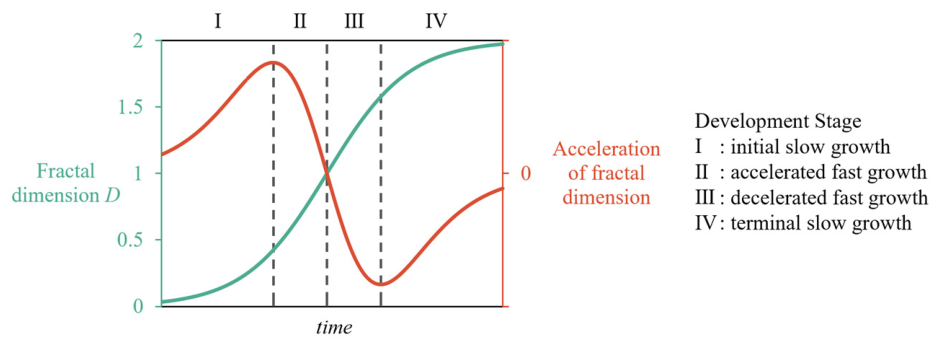
Modeling fractal-related parameters with Logistic functions allows the prediction of future evolution trends and the identification of development stages [41]. Specifically, based on the extrema and zero-crossing points of the Logistic function’s acceleration, the evolution process can be divided into four stages (see Figure 3): Stage I—Initial slow growth; Stage II—Accelerated fast growth; Stage III—Decelerated fast growth; Stage IV—Terminal slow growth. To ensure the reliability of the model, the goodness-of-fit R² of the Logistic function is evaluated, serving as a robustness check for the time-series modeling results.

On the other hand, to identify the primary driving factors of railway development in urban systems, this study employs stepwise regression modeling for the correlation dimension D_c. D_c reflects the degree of intercity correlation based on railway travel times and is influenced by factors such as railway infrastructure and train operation arrangements [23]:

• Railway infrastructure: Improvements in correlation are associated with the expansion of the railway line and increases in the number of stations. In this study, the capacity dimension of railway line spatial distribution D_b and the annual number of stations N_s are used as proxies.
• Train operations: Enhancements in correlation are linked to higher train speeds and increased direct services. Following approaches from complex network analysis, the average train running time T_mean is used as a proxy for train speed, which is inversely related to T_mean, and the number of direct services L_direct is used to represent the frequency of direct services.

Scientific research fundamentally aims at both explanation and prediction [42,43]. Over relatively short periods, D_c can be approximated as linearly dependent on the above factors, allowing the construction of a multiple stepwise regression model. For prediction, a multiple linear regression model of D_c can be constructed directly from the original variables:

$$D_c(t)={\alpha }_0+{\alpha }_1\times D_b(t)+{\alpha }_2\times N_s(t)+{\alpha }_3\times T_{\mathrm{mean}}(t)+{\alpha }_4\times L_{\mathrm{direct}}(t),$$

(9)

where α_i (i = 0, 1, 2, 3, 4) are coefficients, with α₃ < 0 and α₁, α₂, α₄ > 0 theoretically. For explanatory purposes, a regression model can be established based on standardized variables:

$$D_c^{*}(t)={\beta }_1\times D_b^{*}(t)+{\beta }_2\times N_s^{*}(t)+{\beta }_3\times T_{\mathrm{mean}}^{*}(t)+{\beta }_4\times L_{\mathrm{direct}}^{*}(t),$$

(10)

where “*” denotes standardized variables. The constant term is 0, and β_i (i = 1, 2, 3, 4) are standardized regression coefficients, reflecting the relative influence of each independent variable. Larger β_i indicate a more significant effect on D_c.

For the regression analysis above, a significance level of p = 0.05 is adopted, and parameters are estimated using OLS.

2.3. Study Area and Data Processing

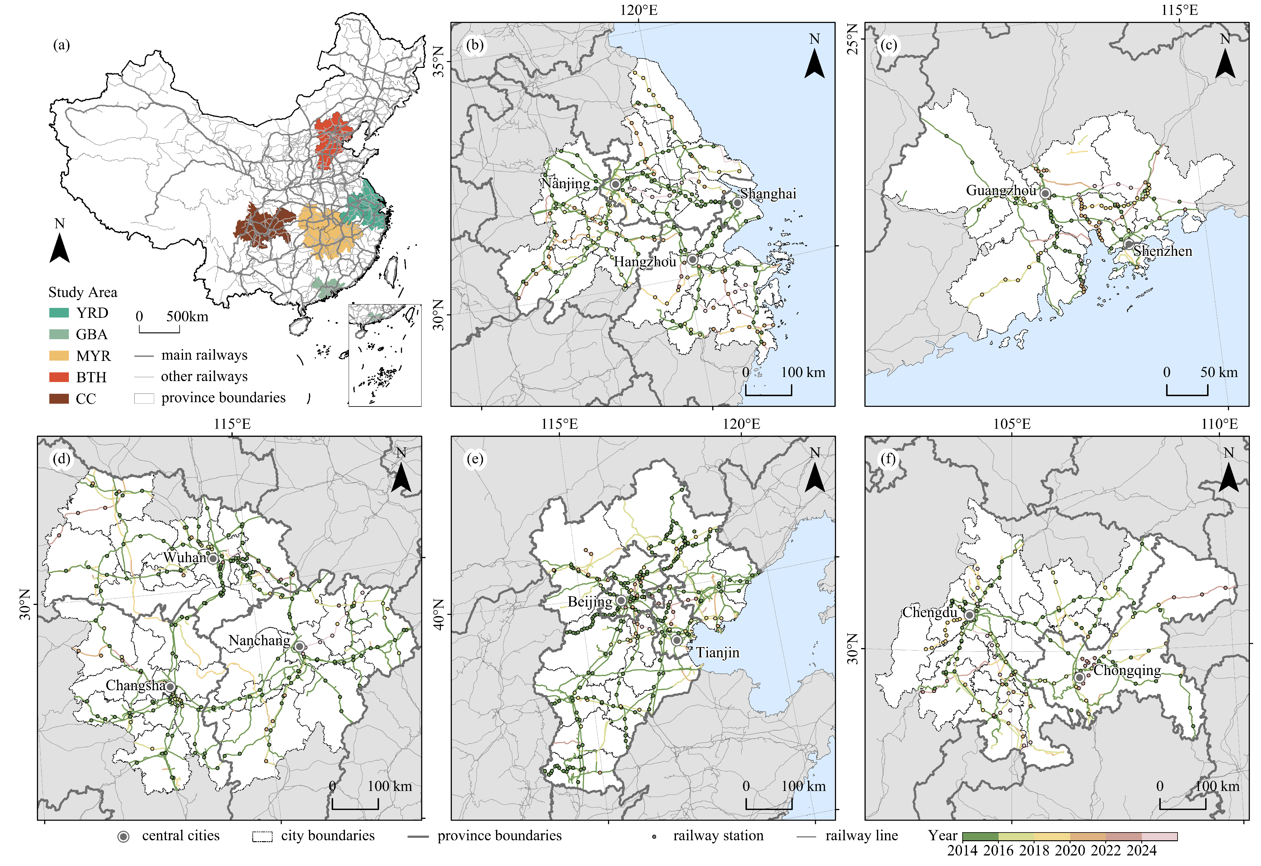
This study employs a fractal-based framework to analyze the spatial distribution, temporal correlations, evolutionary trends, and driving factors of railway networks in China’s five major urban systems. The study objects are the national-level urban systems: the Yangtze River Delta (YRD), the Guangdong–Hong Kong–Macao Greater Bay Area (GBA), the Middle Yangtze River (MYR), the Beijing-Tianjin-Hebei region (BTH), and the Chengdu-Chongqing region (CC). The spatial boundaries of the urban systems in this study are based on relevant national development plans, encompassing 4 municipalities, 2 special administrative regions (SARs), and 91 prefecture-level cities (PLCs) across 9 provinces (Figure 4,

Table 2. Basic characteristics of railway networks in five major urban systems (based on 2024 data).

	YRD 1	GBA	MYR	BTH	CC
Constituent regions	Shanghai (municipality); 9 PLCs in Jiangsu; 8 in Zhejiang; 8 in Anhui.	9 PLCs in Guangdong; Hong Kong SAR; Macao SAR.	13 PLCs in Hubei; 8 in Hunan; 10 in Jiangxi.	Beijing; Tianjin (both municipalities); 11 PLCs in Hebei.	Chongqing (municipality); 15 PLCs in Sichuan.
Central cities	Shanghai, Nanjing, Hangzhou	Guangzhou, Shenzhen	Wuhan, Changsha, Nanchang	Beijing, Tianjin	Chongqing, Chengdu
GDP (trillion CNY)	27.64	14.79	14.74	11.50	8.70
Area (km2)	209,378	59,975	352,925	203,054	239,222
Network length (km)	19,233	6979	26,097	28,580	11,985
Ns 2	182	110	206	228	154
Ldirect 3	7581	1481	5597	4560	2763
Network density (km/km2)	0.0919	0.1164	0.0739	0.1407	0.0501
Station density (stations/km2)	8.6924	18.3411	5.8369	11.2286	6.4375
β index	41.6538	13.4636	27.1699	20.0000	17.9416

¹ YRD = Yangtze River Delta; GBA = Guangdong–Hong Kong–Macao Greater Bay Area; MYR = Middle Yangtze River region; BTH = Beijing–Tianjin–Hebei region; CC = Chengdu–Chongqing region. ² the number of stations. ³ the number of direct services.

). Despite covering only about 10% of China’s land area, they account for more than 55% of national GDP and over 60% of the country’s railway mileage, making them the most densely connected railway regions in China. Based on the 2024 statistics (Table 2 and Table S1, Figure S1), the five urban systems exhibit clear differences in railway network characteristics. In absolute terms, BTH and MYR show relatively larger network scales (network length and number of stations), whereas CC and GBA are smaller, with the latter largely constrained by its limited area. In terms of density, BTH and GBA rank highest, particularly GBA, which demonstrates a markedly higher station density than the others, while CC remains relatively low. Regarding connectivity (β index), YRD significantly outperforms the other regions, whereas GBA shows comparatively weaker network connectivity.

Regarding data sources, this study uses railway line data and train timetable data to represent the spatial distribution and temporal correlations of the railway network. Railway line data were obtained from OpenStreetMap (global platform; data extracted for China) (https://www.openstreetmap.org/), while train timetable data were sourced from the National Railway Timetable (Beijing, China: China Railway Publishing House) and the China Railway 12306 website (Beijing, China) (https://www.12306.cn/). Both datasets cover the period 2014–2024 (Figure 4).

The specific calculation procedures are as follows (Figure 2b):

• Spatial distribution analysis: The functional box method and Equation (2) are used to compute the capacity dimension D_b of railway line distribution. Specifically, for each study area, the minimum bounding rectangle is first determined. The rectangle is then subdivided into nine levels, with the scale r ranging from several hundred kilometers to approximately 1 km (see Figure 5a). Subsequently, capacity dimension D_b is estimated based on Equation (2).
• Temporal correlation analysis: The shortest travel times between all stations within each urban system are calculated and used as d_ij in Equations (3) and (6). Travel time is derived from train timetables, considering both direct railway connections and transfer routes. Transfers are restricted to within the same city. For each transfer, the departure time of the subsequent leg must be at least 3 min later than the arrival time of the previous leg, and the waiting time is included in the total travel time. For inter-station transfers within a city, travel time between the stations is approximated by driving time based on data from the Baidu Maps Open Platform (https://lbsyun.baidu.com/), and such transfers are considered valid only if the time interval between consecutive legs exceeds the corresponding driving time. Under these constraints, the minimum travel time among all feasible routes is determined as d_ij. Subsequently, the radius method and Equations (5) and (6) are applied to compute the radial dimension D_α and correlation dimension D_c of railway temporal correlation.
• Regression analysis of fractal parameters: For each urban system, the temporal evolution of fractal parameters across different years is first fitted with Logistic functions Equations (7) and (8) to predict future trends and divide urban development stages. Then, treating the correlation dimension D_c as the dependent variable and the capacity dimension D_b, number of stations N_s, average train running time T_mean, and number of direct services L_direct as independent variables, a multiple stepwise regression model is constructed to identify the main driving factors of D_c using Equations (9) and (10).

The data are processed and calculated using Python 3.8.

3. Results

3.1. Analysis of Spatial Pattern

Based on railway line data, the box method was used to calculate the capacity dimension D_b of the spatial distribution of railway networks. In the log–log plots of S(r) versus r (partial results shown in Figure 5a), the data points exhibit a clear linear relationship, with the goodness of fit R² > 0.97, indicating that the spatial pattern of railway networks in the five major urban systems possesses fractal properties. The slope of the fitted line was used to estimate D_b (

Table 3. Fractal parameters of the railway spatial distribution in the five major urban systems.

Year	YRD		GBA		MYR		BTH		CC
	Db 1	R2	Db	R2	Db	R2	Db	R2	Db	R2
2014	1.4747	0.9754	1.3293	0.9789	1.5042	0.9738	1.5377	0.9803	1.3730	0.9731
2015	1.4835	0.9771	1.3615	0.9780	1.5392	0.9755	1.5502	0.9813	1.4308	0.9792
2016	1.4920	0.9785	1.3758	0.9755	1.5501	0.9767	1.5607	0.9814	1.4667	0.9790
2017	1.5031	0.9775	1.3893	0.9755	1.5616	0.9775	1.5830	0.9835	1.4809	0.9791
2018	1.5079	0.9779	1.3817	0.9775	1.5643	0.9762	1.5799	0.9832	1.4870	0.9794
2019	1.5117	0.9778	1.3907	0.9798	1.5703	0.9767	1.5828	0.9832	1.4891	0.9789
2020	1.5167	0.9777	1.3915	0.9803	1.5802	0.9775	1.5874	0.9839	1.4937	0.9794
2021	1.5286	0.9773	1.4009	0.9809	1.5810	0.9776	1.5890	0.9840	1.4925	0.9774
2022	1.5420	0.9780	1.4177	0.9822	1.5864	0.9771	1.5667	0.9807	1.5019	0.9768
2023	1.5432	0.9783	1.4185	0.9823	1.5882	0.9780	1.5961	0.9842	1.5071	0.9773
2024	1.5520	0.9790	1.4290	0.9829	1.5923	0.9782	1.5965	0.9844	1.5197	0.9790
AAGR 2	0.51%		0.73%		0.57%		0.38%		1.02%

¹ all parameters above pass the test at the 0.05 significance level. ² the Annual Average Growth Rate over the study period.

). The results show that the BTH and MYR railway networks have the highest D_b values and the most intensive spatial coverage, whereas the GBA network exhibits the lowest D_b and the weakest spatial filling. Overall, the D_b values of the five urban systems show a slow upward trend, with an annual average growth rate (AAGR) of approximately 1%. Among them, BTH shows the lowest growth rate (0.38%), suggesting that its railway network spatial structure has become relatively mature.

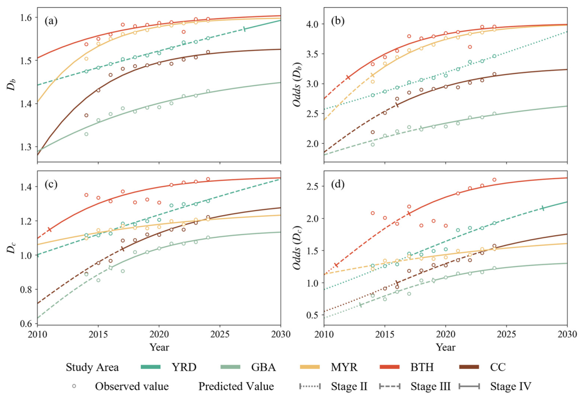
Further, the temporal evolution of the capacity dimension D_b and its fractal odds ratio was fitted using a Logistic function, as shown in

Table 4. Logistic modeling results for the fractal parameters of railway spatial distribution in the five major urban systems.

Urban System	Db			Odds Ratio
	Model 1	R2	Development Stage	Model	R2	Development Stage
YRD	$D_b(t)={\displaystyle \frac{1.99}{1+{\mathrm{e}}^{41.21-0.02t}}}$	0.9870	III: 2014~2027	$Odds(t)={\displaystyle \frac{9.61}{1+{\mathrm{e}}^{62.59-0.03t}}}$	0.9862	II
GBA	$D_b(t)={\displaystyle \frac{1.48}{1+{\mathrm{e}}^{191.80-0.10t}}}$	0.9266	IV	$Odds(t)={\displaystyle \frac{2.83}{1+{\mathrm{e}}^{198.08-0.10t}}}$	0.9266	III: 2014~2018 IV: 2019–2024
MYR	$D_b(t)={\displaystyle \frac{1.60}{1+{\mathrm{e}}^{465.01-0.23t}}}$	0.9840	IV	$Odds(t)={\displaystyle \frac{4.01}{1+{\mathrm{e}}^{451.21-0.22t}}}$	0.9841	III: before–2014 IV: 2015–2024
BTH	$D_b(t)={\displaystyle \frac{1.61}{1+{\mathrm{e}}^{284.99-0.14t}}}$	0.6991	IV	$Odds(t)={\displaystyle \frac{4.01}{1+{\mathrm{e}}^{456.50-0.23t}}}$	0.7098	III: before~2012 IV: 2013–2024
CC	$D_b(t)={\displaystyle \frac{1.53}{1+{\mathrm{e}}^{426.23-0.21t}}}$	0.8931	IV	$Odds(t)={\displaystyle \frac{3.29}{1+{\mathrm{e}}^{387.92-0.19t}}}$	0.8959	III: 2014~2016 IV: 2017–2024

¹ all parameters above pass the test at the 0.05 significance level.

and Table S2 and Figure 6a,b. The numerator of the function represents the theoretical upper limit of the fractal parameter describing the spatial distribution of regional railway networks. The upper limit of D_b for the YRD is approximately 1.99, with the 2024 value reaching about 78% of this limit, indicating that the spatial filling of its railway network still has room for growth. In contrast, the D_b values of the other urban systems in 2024 have exceeded 95% of their respective upper limits, suggesting that their spatial distribution patterns have become largely stable. The Logistic curves also reveal the staged evolution of the railway spatial distribution patterns. The D_b of the YRD is currently in the decelerated fast growth phase (Stage III) and is expected to stabilize around 2027. The other urban systems have already entered the terminal slow growth phase (Stage IV). However, the evolution of the fractal odds ratio shows some variations: The BTH and MYR networks entered Stage IV in 2012 and 2014, respectively, indicating that their inward filling processes were completed earlier and their spatial structures have been largely finalized. The CC and GBA networks, after experiencing decelerated fast growth, entered Stage IV in 2016 and 2018, respectively. This implies that the early development of their regional railway networks was dominated by inward filling, and by the end of the study period, their spatial distribution patterns had stabilized and become largely fixed.

3.2. Analysis of Temporal Correlation

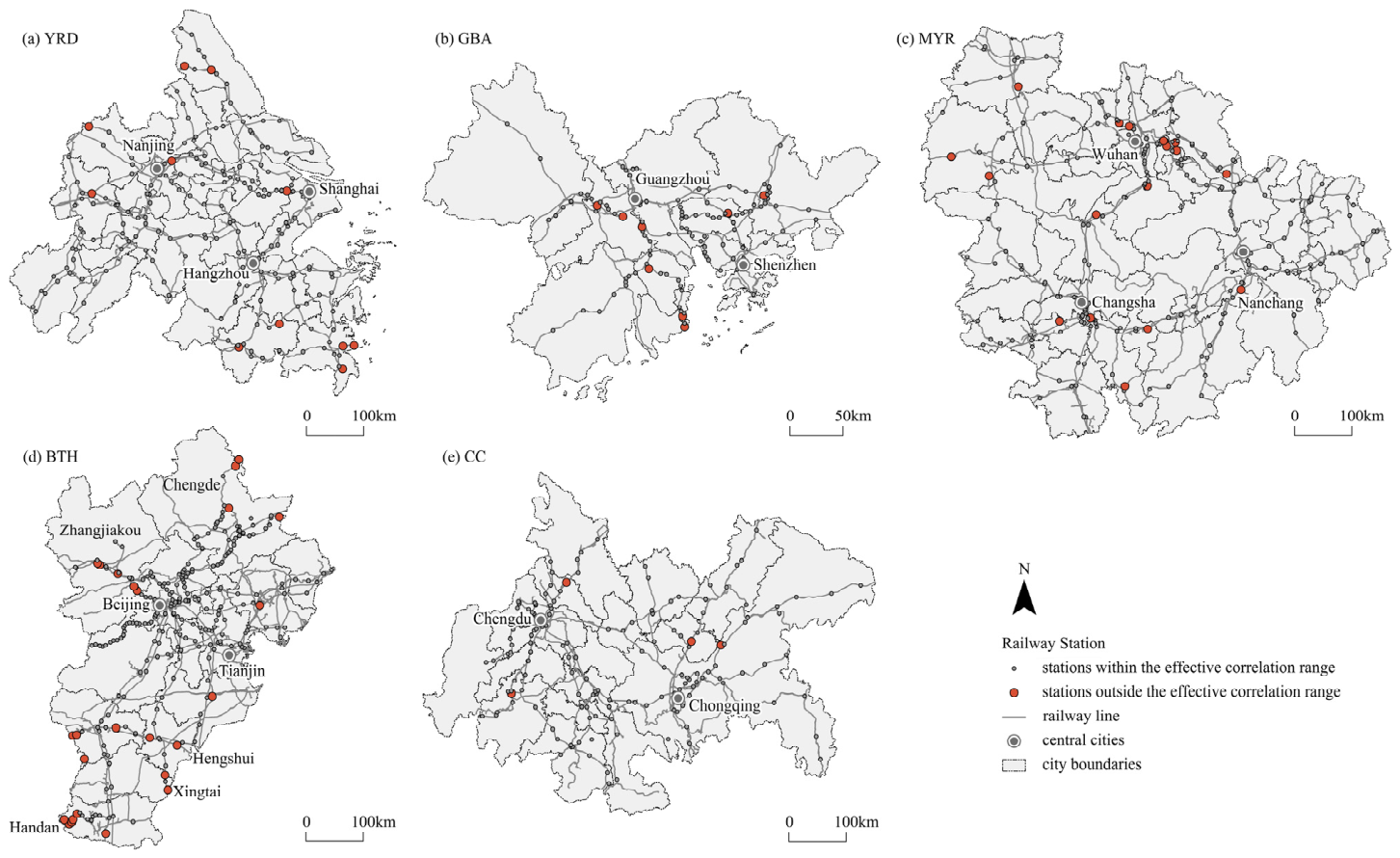
Based on the railway timetable data, the correlation dimension D_c and radial dimension D_α of the railway time correlation were calculated using the radius method. In the log–log plots for calculating D_c (partial results shown in Figure 5b), the scatter points of the correlation function C(r) against scale r exhibit an S-shaped distribution, with a clearly linear segment in the middle. This indicates that the railway networks of the five major urban systems all exhibit fractal structures in the scaling range of time correlation. Specifically (

Table 5. Identification of scaling ranges in railway temporal correlation for the five major urban systems.

	YRD	GBA	MYR	BTH	CC
Scaling Range	5 min–6.1 h	3 min–4 h	9 min–10.7 h	18 min–5 h	6 min–8.1 h
Central City Coverage 1	94.39%	93.33%	92.67%	90.23%	97.55%

¹ proportion of stations within the effective temporal correlation range of central cities.

), the scaling ranges of MYR and CC are the longest, with effective time correlation ranges of approximately 10 min–9 h. The scaling ranges of YRD and GBA are slightly shorter but have smaller lower bounds (around 5 min), suggesting closer inter-station connections within the region. In contrast, BTH shows the shortest scaling range and a limited effective time correlation range, indicating that the fractal characteristics of its temporal correlation are not yet fully developed across the region. By calculating the proportion of stations within the effective time correlation range of central cities in 2024 (Table 5, Figure 7), it is found that the central cities of YRD, GBA, MYR, and CC have high coverage levels, all exceeding 92%, spatially covering almost the entire region except for a few peripheral areas. This suggests that, except for a few marginal cities, regional railway transport has largely achieved temporal integration. In contrast, BTH shows a slightly lower central city coverage rate (90.23%); its northern (Chengde and Zhangjiakou) and southern peripheral cities (Hengshui, Xingtai, and Handan) remain outside the effective correlation range, indicating that the degree of temporal integration of its regional railway system still needs improvement.

By estimating the slope of scatter points within the scaling range, the temporal correlation dimension D_c was obtained (

Table 6. Fractal parameters of the railway temporal correlation in the five major urban systems.

Year	YRD		GBA		MYR		BTH		CC
	Dc 1	R2	Dc	R2	Dc	R2	Dc	R2	Dc	R2
2014	1.1175	0.9942	0.8881	0.9965	1.0980	0.9950	1.3516	0.9956	0.8923	0.9794
2015	1.1155	0.9943	0.8537	0.9604	1.1473	0.9951	1.3352	0.9959	0.9547	0.9936
2016	1.1264	0.9953	0.9259	0.9935	1.1478	0.9950	1.3150	0.9971	0.9674	0.9957
2017	1.1848	0.9932	0.9074	0.9851	1.1712	0.9937	1.3720	0.9959	1.0849	0.9908
2018	1.1802	0.9953	1.0177	0.9958	1.1592	0.9911	1.3085	0.9970	1.0876	0.9919
2019	1.1984	0.9948	1.0181	0.9955	1.1565	0.9910	1.3246	0.9975	1.1217	0.9909
2020	1.2069	0.9944	1.0401	0.9939	1.1651	0.9923	1.3076	0.9976	1.1192	0.9915
2021	1.2906	0.9947	1.0683	0.9922	1.1991	0.9901	1.4099	0.9964	1.1498	0.9907
2022	1.2989	0.9940	1.0682	0.9925	1.1797	0.9914	1.4240	0.9958	1.1494	0.9899
2023	1.2981	0.9940	1.0766	0.9927	1.2078	0.9893	1.4303	0.9961	1.1887	0.9907
2024	1.3167	0.9934	1.1033	0.9904	1.2091	0.9906	1.4452	0.9944	1.2234	0.9896
AAGR 2	1.65%		2.19%		0.97%		0.67%		3.21%

¹ all parameters above pass the test at the 0.05 significance level. ² the Annual Average Growth Rate over the study period.

). The results show that D_c in all urban systems exhibits an overall fluctuating upward trend, though growth rates differ. CC shows the fastest increase, with D_c rising from the lowest value in 2014 to the third highest in 2024, corresponding to an AAGR exceeding 3%. GBA follows with approximately 2.2%, while MYR and BTH grow the slowest, at less than 1%. This indicates that the spatiotemporal compression effect is most pronounced in CC, whereas it is relatively weak in MYR and BTH. Nevertheless, due to the large initial differences in D_c among the five urban systems, a stable hierarchical distribution pattern of D_c is maintained overall: BTH exhibits the highest temporal correlation, GBA the lowest, with YRD, CC, and MYR occupying intermediate positions.

The temporal evolution of the correlation dimension D_c and its fractal odds ratio was fitted using the Logistic model, with results shown in

Table 7. Results of Logistic modeling for the fractal parameters of railway temporal correlation in the five major urban systems.

Urban System	Dc			Odds Ratio
	Model 1	R2	Development Stage	Model	R2	Development Stage
YRD	$D_c(t)={\displaystyle \frac{1.99}{1+{\mathrm{e}}^{96.17-0.05t}}}$	0.9380	III	$Odds(t)={\displaystyle \frac{2.75}{1+{\mathrm{e}}^{226.75-0.11t}}}$	0.9264	II: 2014~2017 III: 2018~2024
GBA	$D_c(t)={\displaystyle \frac{1.15}{1+{\mathrm{e}}^{408.70-0.20t}}}$	0.9443	III: 2014~2016 IV: 2017~2024	$Odds(t)={\displaystyle \frac{1.34}{1+{\mathrm{e}}^{424.96-0.21t}}}$	0.9445	II: before~2013 III: 2014~2019 IV: 2020~2024
MYR	$D_c(t)={\displaystyle \frac{1.27}{1+{\mathrm{e}}^{187.58-0.09t}}}$	0.8251	IV	$Odds(t)={\displaystyle \frac{1.75}{1+{\mathrm{e}}^{183.68-0.09t}}}$	0.8251	III: 2014~2018 IV: 2019~2024
BTH	$D_c(t)={\displaystyle \frac{1.46}{1+{\mathrm{e}}^{398.73-0.20t}}}$	0.6228	IV	$Odds(t)={\displaystyle \frac{2.67}{1+{\mathrm{e}}^{451.30-0.22t}}}$	0.6243	III: 2014~2017 IV: 2018~2024
CC	$D_c(t)={\displaystyle \frac{1.32}{1+{\mathrm{e}}^{321.73-0.16t}}}$	0.9476	III: 2014~2017 IV: 2018~2024	$Odds(t)={\displaystyle \frac{1.92}{1+{\mathrm{e}}^{329.54-0.16t}}}$	0.9477	II: 2014~2016 III: 2017~2024 IV: 2025~after

¹ all parameters above pass the test at the 0.05 significance level.

and Table S2 and Figure 6c,d. The numerator of the function corresponds to the theoretical upper limit of the regional railway temporal correlation fractal parameter. The results indicate that the upper limit of D_c in the YRD is approximately 1.99, with the 2024 value reaching around 66% of this limit, suggesting that there is still potential for further temporal correlation growth in its railway network. In contrast, the D_c values of the other urban systems in 2024 have already exceeded 92% of their theoretical limits, indicating that the regional railway spatiotemporal compression is approaching its maximum. The Logistic curves further reveal the staged evolution of railway temporal correlation patterns. D_c in the YRD is currently in Stage III, indicating room for future improvement. CC and GBA experienced Stage III in the early period and entered Stage IV in 2017 and 2016, respectively. Specifically, the fractal odds ratio in CC transitioned from Stage II to III in 2016 and reached IV by 2024, whereas in GBA, it shifted from Stage II to III around 2013 and reached IV by 2019. This indicates that the temporal correlation in CC and GBA stabilized by the mid-study period, with GBA developing faster and stabilizing earlier. By contrast, MYR and BTH have remained in Stage IV since the early period of the study, with their fractal odds ratios stabilizing in 2018 and 2017, respectively, indicating that their temporal correlation patterns have largely matured, leaving limited room for further growth.

A comparison between the spatial capacity dimension D_b and the temporal correlation dimension D_c highlights the distinct developmental stages of regional railway networks. Overall, D_c values are lower than D_b and reach later development stages, but their growth rates during the study period are higher. In the YRD, both D_b and D_c remain in Stage III, with D_b expected to stabilize around 2027, whereas D_c continues in the decelerated fast growth phase. In MYR and BTH, both D_b and D_c are in Stage IV; however, the fractal odds ratios first grow rapidly and then stabilize, with the D_c odds ratio entering Stage IV approximately five years later than that of D_b. In GBA and CC, D_b has already reached Stage IV, while D_c initially grows rapidly and then stabilizes, with the entry of its fractal odds ratio into Stage IV lagging behind D_b. Specifically, in GBA, the stabilization of the D_b and D_c odds ratios differs by only one year, indicating the most synchronous evolution of spatial distribution and temporal correlation. By contrast, in CC, the lag effect is most pronounced, with an eight-year difference. Notably, the D_b odds ratio enters Stage IV in the same year (2017) that the D_c odds ratio enters Stage III, reflecting a typical “space-first, time-lagged” staged development pattern of the regional railway network.

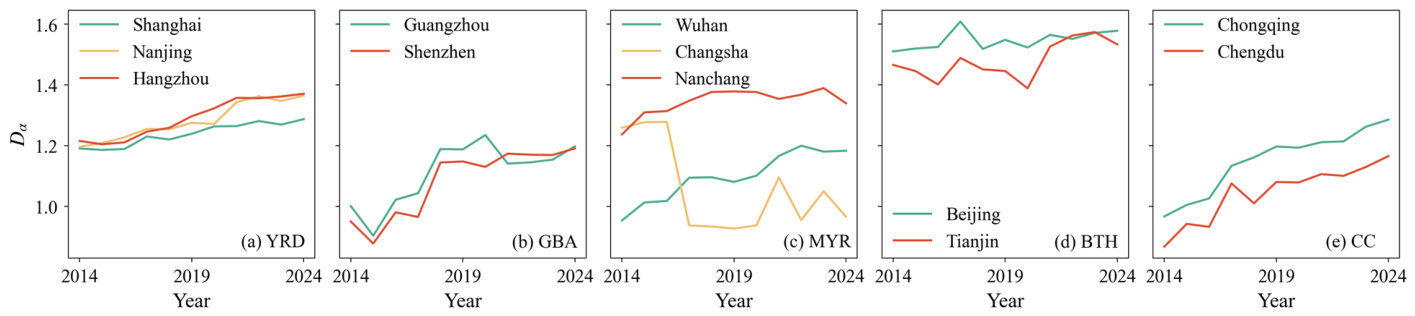
In addition, the radial dimension D_α of central cities in each urban system was calculated to reveal the temporal correlation characteristics between central and surrounding cities. Similar to the correlation dimension, D_α was computed within the previously identified scaling range, with partial processes shown in Figure 5c. In the log–log plots of C_i(r) versus r, scatter points for all central cities exhibit clear linear patterns, with linear regression goodness-of-fit R² > 0.77, indicating that the temporal correlations between central and surrounding cities still display fractal features. Further analysis of the temporal evolution of D_α for each central city (Figure 8, Table S3) shows that all values are below 2, reflecting a general centripetal tendency. However, the degree of clustering varies, resulting in distinct aggregation structures. In the YRD, D_α values of Shanghai, Nanjing, and Hangzhou were initially similar. Over time, D_α for Nanjing and Hangzhou gradually increased and approached each other, suggesting that the regional clustering structure evolved from a three-core pattern of “Shanghai–Nanjing–Hangzhou” into a hierarchical structure of “Shanghai–Nanjing and Hangzhou” with one primary core and two secondary wings. In the GBA and BTH, D_α values for Guangzhou and Shenzhen, and for Beijing and Tianjin, remained consistently similar, forming a stable dual-core pattern of “Guangzhou–Shenzhen” and “Beijing–Tianjin,” respectively. In the MYR, Wuhan initially had a smaller D_α, while Changsha and Nanchang had larger, comparable values. After the addition of seven new stations in Changsha in 2017, its D_α decreased to below that of Wuhan, indicating a rapid increase in centripetal temporal correlation and a structural shift from a “Wuhan–Changsha and Nanchang” one-core–two-wing pattern to a three-tier pattern of “Changsha–Wuhan–Nanchang”. In the CC, Chengdu’s D_α consistently remained smaller than Chongqing’s, forming a primary–secondary core relationship of “Chengdu–Chongqing”.

3.3. Analysis of Factors for Temporal Correlation

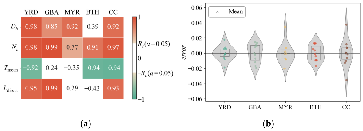
To identify the main factors influencing the temporal correlation dimension D_c of the five major urban systems, a multiple stepwise regression model was established. First, the correlation coefficients between D_c and various influencing factors were calculated to preliminarily assess the model’s validity (Figure 9a, Table S4). The results show that, at the 0.05 significance level, D_c is significantly correlated with most factors, confirming the rationality of Equation (9). Based on stepwise regression modeling (

Table 8. Stepwise multiple regression results of railway temporal correlation dimension in the five major urban systems.

Urban System	Variables	αi 1	βi	R2	Urban System	Variables	αi	βi	R2
YRD	const	−0.967		0.9851	BTH	const	1.388		0.9297
	Ns	0.002	0.578			Tmean	−0.001	−0.583
	Db	1.298	0.426			Ns	0.002	0.423
GBA	const	0.793		0.9857	CC	const	−0.430		0.9706
	Ns	0.003	0.993			Ns	0.002	0.675
MYR	const	−0.608		0.8533		Db	0.860	0.342
	Db	1.134	0.924

¹ “const” denotes the constant term, α_i denotes the regression coefficient, and β_i denotes the standardized regression coefficient. All parameters above pass the test at the 0.05 significance level.

and Table S4, Figure 9b), the main influencing factors of D_c in each urban system are generally one or two variables. The models exhibit goodness-of-fit values exceeding 0.85 and all pass the 0.05 significance test.

According to the differences in influencing factors, the five urban systems can be roughly classified into three types: (1) Station-increase type. The variation in D_c is mainly driven by the increase in the number of stations (N_s), represented by the YRD, GBA, and CC. Among them, the YRD and CC show rapid D_c growth during the study period, jointly influenced by N_s and the spatial capacity dimension D_b, with N_s having a stronger standardized effect. The influence of N_s on D_c is particularly prominent in CC. In contrast, GBA exhibits a pattern of rapid early growth followed by stabilization, mainly driven by N_s. (2) Network-expansion type: The variation in D_c is mainly affected by the expansion of railway lines (D_b), as observed in MYR. Both D_c and D_b in MYR have already stabilized, indicating that further enhancement of temporal correlation primarily depends on continued inward densification of the railway network. (3) Train-speed-improvement type. The variation in D_c is influenced by the increase in average train speed (i.e., the reduction in mean travel time T_mean), represented by BTH. N_s also plays a role, though its effect is weaker than that of T_mean. As D_c in BTH has already stabilized, further improvement in temporal correlation mainly results from the spatiotemporal compression effect induced by higher train speeds and the addition of new stations.

4. Discussion

Under the guidance of policies such as the “National Comprehensive Three-Dimensional Transportation Network Planning Outline”, the construction of China’s transportation network has accelerated significantly, and railways have played a crucial role in supporting the coordinated development and spatial integration of urban systems. Against this background, examining the spatial distribution and temporal correlation patterns of railway networks in China’s major urban systems is of great significance. Using two fractal analysis methods, this study systematically explores the spatial structure, temporal correlation characteristics, and their evolutionary trends and driving factors in railway networks. The main findings are summarized as follows:

• Both the spatial distribution and temporal correlation of railway networks across the five major urban systems show an overall upward trend, but the development of temporal correlation lags behind spatial filling by approximately 1–8 years. The railway networks exhibit typical fractal structures in both spatial distribution and temporal correlation. Their corresponding spatial capacity dimension D_b and temporal correlation dimension D_c both increase over time, reflecting enhanced spatial compactness and temporal accessibility. However, D_c reaches the terminal slow growth phase (Stage IV) later than D_b but grows at a faster rate, indicating that temporal correlation develops more slowly than spatial expansion but accelerates more rapidly during the study period. In the YRD, spatial expansion is projected to stabilize around 2027, transitioning toward internal densification, while temporal correlation remains in a decelerated fast growth phase (Stage III). In the other urban systems, both D_b and D_c have stabilized by the end of the study period, though the onset of stabilization differs, reflecting varying degrees of asynchrony. Among them, the GBA exhibits the highest synchronicity, with only a one-year difference between the stabilization of D_b and D_c. In MYR and BTH, D_c lags D_b by approximately five years. In contrast, CC shows the most pronounced lag, up to eight years: its D_b enters Stage IV in the same year (2017) when D_c enters Stage III, reflecting a typical “space-first, time-lagged” phased development pattern of the regional railway network.
• The development levels, integration degrees, and agglomeration structures of railway networks vary considerably among the five urban systems. In general, the YRD shows the greatest growth potential, while the MYR has the least; the BTH is the most developed but also the most concentrated; the GBA and CC are developing the fastest. The YRD’s railway network demonstrates rapid growth in both spatial distribution and temporal correlation, with the latest stabilization time among all urban systems, indicating the greatest remaining potential. Its internal network connections are dense, forming a multi-level agglomeration pattern centered on Shanghai, with Nanjing and Hangzhou as two secondary cores. In contrast, the MYR’s spatial filling and temporal correlation both stabilized early, showing limited future potential. Its temporal correlation forms a hierarchical structure of “Changsha–Wuhan–Nanchang,” where central cities have wide radiation ranges but overall low correlation levels. The BTH network is highly concentrated around Beijing and Tianjin. It is the most developed in both spatial and temporal dimensions but has the lowest degree of integration. Its temporal correlation exhibits a dual-core pattern of “Beijing–Tianjin”, with strong internal connections but limited spatial coverage, excluding northern (Chengde, Zhangjiakou) and southern (Hengshui, Xingtai, Handan) peripheral cities. The GBA and CC networks have relatively low overall levels of spatial filling and temporal correlation but the fastest growth rates, with fractal parameters rising sharply in the early stage and stabilizing around 2017. The GBA forms a dual-core pattern of “Guangzhou–Shenzhen”, characterized by tight station connectivity and highly synchronized evolution between spatial and temporal structures. The CC, however, presents a “Chengdu–Chongqing” main–sub core structure, with broader radiation from core cities but a more significant lag in temporal correlation relative to spatial distribution.
• The temporal correlation of railway networks across the five urban systems is mainly influenced by three factors—station increase, network expansion, and train-speed improvement—though the dominant factor varies by region. Accordingly, the urban systems can be categorized into three types: (a) Station increase type: The variation in D_c is primarily driven by the increase in the number of stations (N_s), as seen in the YRD, GBA, and CC. Among them, D_b also exerts influence in the YRD and CC, but to a lesser extent. (b) Network expansion type: The variation in D_c mainly results from railway network expansion (D_b), represented by the MYR. Both D_b and D_c in the MYR have stabilized, suggesting that further improvement in temporal correlation depends on inward densification and structural optimization of the network. (c) Train-speed improvement type: The variation in D_c is mainly influenced by the increase in average train speed (i.e., the reduction in mean travel time T_mean), represented by the BTH. Station increase also has a secondary effect. Since D_c in the BTH has already stabilized, subsequent improvement in temporal correlation primarily arises from the spatiotemporal compression effect jointly induced by higher train speeds and the addition of new stations.

As the “blood vessels” and “skeleton” of urban systems, transportation networks have long been a central focus of academic research. Fractal methods are widely used to characterize their scaling properties. Existing studies mainly fall into two categories: physical network studies, which examine spatial filling and heterogeneity [4,6,7,10], and service network studies, which focus on accessibility and flow patterns [8,9,14,17]. In addition, complex network approaches are often used to analyze structural features such as community structure and hub roles [44,45]. Although these studies collectively demonstrate the complexity of transportation networks from multiple perspectives, most of them remain confined to either the physical or the service layer. Some studies attempt to integrate multiple dimensions—such as physical, service, and topological characteristics—when analyzing railway, metro, or street networks [1,8,18]. However, a unified analytical framework is still lacking, and systematic comparative analysis and the exploration of evolutionary dynamics remain insufficient.

In contrast, the main innovations of this study lie in two aspects. First, it develops a fractal-based analytical framework from a dual “space–time” perspective, integrating spatial distribution (physical structure) and temporal correlation (service interaction). Second, by leveraging the time-series modeling and factor-identification capabilities of fractal analysis, this study predicts future development trends of transportation networks and reveals their key driving factors. Through cross-perspective comparison of fractal parameters, the study provides a more systematic understanding of the evolutionary processes and stage-division characteristics of transportation networks.

From a policy perspective, China is actively promoting the integrated development of its transportation system. The “National Comprehensive Three-Dimensional Transportation Network Planning Outline (2021)” emphasizes improving infrastructure across multiple transport modes while establishing a railway-oriented backbone for the national integrated transport network. It also highlights the importance of promoting the coordinated development of trunk railways, intercity railways, and suburban (commuter) railways, with the goal of forming a unified “one network” for operation, management, and services. The framework proposed in this study closely aligns with this policy orientation by explicitly linking infrastructure configuration (spatial structure) with service performance (temporal efficiency), thereby providing an analytical basis for integrating construction and operation within a unified evaluation system. Empirical findings in this study provide both a methodological framework and practical insights for improving railway networks. In particular, they suggest that infrastructure development and service optimization should be advanced in a more coordinated manner: regions with relatively mature spatial structures should shift policy focus toward enhancing service efficiency, strengthening inter-station connectivity, and improving time-based accessibility. More broadly, by integrating spatial and temporal perspectives, this study supports the transition from scale expansion to efficiency-oriented development, offering a scientific basis for the coordinated optimization of infrastructure and service networks in line with national transport strategies.

Although this study makes several innovative contributions, there are still some limitations. First, due to the limited temporal coverage of the datasets, the results of the time-series analysis may contain some uncertainties. With improvements in data quality, future studies could incorporate longer time series to enhance analytical accuracy. Second, this study focuses solely on railway networks, without including highway, aviation, or waterway systems. Given the differences in geographical conditions and transport structures among various urban systems, highways, waterways, and air transport play irreplaceable roles in regional transport systems. Future research could therefore adopt a multimodal framework to examine the coordinated evolution of integrated transport networks. Third, the study scope is mainly confined to intra-urban system networks, without considering inter-urban system connections or linkages with surrounding regions. Considering that the coordinated development of interregional transport networks is crucial for understanding the overall evolution of urban systems, future research could expand the spatial scope to explore the coupling relationships and evolutionary mechanisms of transport networks at broader scales.

5. Conclusions

Railways constitute a core component of the backbone of the comprehensive three-dimensional transportation network. The evolution of their spatial organization and temporal accessibility directly affects the level of transport integration within urban systems and the operational efficiency of the overall transport system. In the context of China’s ongoing efforts to advance its national integrated transport network and to improve intercity railway systems in key urban systems, systematically identifying the evolutionary patterns of railway networks in terms of spatial expansion and time compression is of both theoretical and practical significance. Drawing on fractal theory, this study examines the structural characteristics, evolutionary trends, and driving factors of railway networks in China’s five major urban systems from 2014 to 2024, from the dual perspectives of spatial distribution and temporal correlation. Based on the foregoing analysis, the main conclusions are as follows.

First, the railway networks of the five urban systems exhibit a staged pattern characterized by “spatial filling preceding temporal correlation”, with a lag of approximately 1–8 years between the two. In terms of spatial filling, most urban systems had already approached stabilization by around 2014, whereas the YRD is projected to maintain rapid growth until approximately 2027. In contrast, temporal correlation shows more heterogeneous dynamics: BTH and MYR stabilized as early as 2014, GBA and CC reached stabilization around 2017, while YRD is expected to remain in a phase of rapid growth. As a result, the temporal lag varies significantly across regions, being approximately 1 year in GBA, 5 years in MYR and BTH, and up to 8 years in CC. This indicates that the realization of network functionality does not coincide with the mere expansion of infrastructure scale. Rather, the transformation from spatial construction to improved temporal accessibility depends on subsequent optimization of operational organization and service capacity, implying the existence of a distinct “function release” period.

Second, a coordinated perspective integrating spatial distribution and temporal correlation enables a more accurate assessment of the functional performance of railway networks and the identification of lagging components. Evaluations should not be confined to whether infrastructure has been constructed, but should further consider whether it effectively compresses regional time distance and enhances transport integration. Based on the stage differences reflected in the two types of fractal parameters, distinct development patterns can be identified across urban systems: YRD exhibits a polycentric structure with the greatest potential; GBA represents an efficiently coordinated type; BTH is highly developed but characterized by dual-core agglomeration; CC shows rapid growth with lagging functional performance; and MYR is axis-dependent with relatively limited potential. For CC and MYR in particular, development strategies should shift from “scale expansion” toward “functional optimization,” with emphasis on inward network densification, improved hub connectivity, more direct service organization, and stronger station–city integration, in order to enhance temporal correlation and regional integration.

Overall, compared with single indicators of network scale, the dual-perspective analytical framework of “spatial distribution–temporal correlation” more effectively captures the actual level of functional performance of railway networks, and provides quantitative support for optimizing national transport systems and promoting high-quality, coordinated development of urban systems.

References

1. Xue, F.; Wang, Z.; Zeng, Y. Research on characteristics of the railway passenger transport network in Chengdu—Chongqing urban agglomeration. J. Beijing Jiaotong Univ. 2025, 49, 17–27. (In Chinese) [Google Scholar]
2. Castells, M. The Informational City: Information Technology, Economic Restructuring, and the Urban-Regional Process; Basil Blackwell: Oxford, UK, 1989. [Google Scholar]
3. Warf, B. Time-Space Compression: Historical Geographies; Routledge: Oxon, UK, 2008. [Google Scholar]
4. Lu, Y.; Tang, J. Fractal dimension of a transportation network and its relationship with urban growth: A study of the Dallas-Fort Worth area. Environ. Plan. B Plan. Des. 2004, 31, 895–911. [Google Scholar] [CrossRef]
5. Thomas, I.; Frankhauser, P. Fractal dimensions of the built-up footprint: Buildings versus roads. Fractal evidence from Antwerp (Belgium). Environ. Plan. B Plan. Des. 2013, 40, 310–329. [Google Scholar] [CrossRef]
6. Murcio, R.; Masucci, A.P.; Arcaute, E.; Batty, M. Multifractal to monofractal evolution of the London street network. Phys. Rev. E 2015, 92, 062130. [Google Scholar] [CrossRef]
7. Long, Y.; Chen, Y. Multifractal scaling analyses of urban street network structure: The cases of twelve megacities in China. PLoS ONE 2021, 16, e0246925. [Google Scholar] [CrossRef]
8. Moreno-Pulido, S.; Pavón-Domínguez, P.; Burgos-Pintos, P. Temporal evolution of multifractality in the Madrid Metro subway network. Chaos Solitons Fractals 2021, 142, 110370. [Google Scholar] [CrossRef]
9. Guo, S.; Pei, T.; Xie, S.; Song, C.; Chen, J.; Liu, Y.; Shu, H.; Wang, X.; Yin, L. Fractal dimension of job-housing flows: A comparison between Beijing and Shenzhen. Cities 2021, 112, 103120. [Google Scholar] [CrossRef]
10. Benguigui, L. A fractal analysis of the public transportation system of Paris. Environ. Plan. A 1995, 27, 1147–1161. [Google Scholar] [CrossRef]
11. Wang, H.; Luo, S.; Luo, T. Fractal characteristics of urban surface transit and road networks: Case study of Strasbourg, France. Adv. Mech. Eng. 2017, 9, 1687814017692289. [Google Scholar] [CrossRef]
12. Ariza-Villaverde, A.B.; Jiménez-Hornero, F.J.; Gutiérrez de Ravé, E. Multifractal analysis applied to the study of the accuracy of DEM-based stream derivation. Geomorphology 2013, 197, 85–95. [Google Scholar] [CrossRef]
13. Pavón-Domínguez, P.; Ariza-Villaverde, A.; Rincón-Casado, A.; de Ravé, E.G.; Jiménez-Hornero, F. Fractal and multifractal characterization of the scaling geometry of an urban bus-transport network. Comput. Environ. Urban Syst. 2017, 64, 229–238. [Google Scholar] [CrossRef]
14. Li, J.; Qian, Y.; Zeng, J.; Yin, F.; Zhu, L.; Guang, X. Research on the influence of a High-speed railway on the spatial structure of the Western Urban Agglomeration based on fractal theory—Taking the Chengdu–Chongqing Urban Agglomeration as an example. Sustainability 2020, 12, 7550. [Google Scholar] [CrossRef]
15. Jiang, B.; Yin, J. Ht-Index for Quantifying the Fractal or Scaling Structure of Geographic Features. Ann. Assoc. Am. Geogr. 2014, 104, 530–540. [Google Scholar] [CrossRef]
16. Long, Y.; Zhai, W.; Shen, Y.; Ye, X. Understanding uneven urban expansion with natural cities using open data. Landsc. Urban Plan. 2018, 177, 281–293. [Google Scholar] [CrossRef]
17. Liu, H.; Shen, Y.; Meng, D.; Xue, J. The City Network Centrality and Spatial Structure in the Beijing-Tianjin-Hebei Metropolitan Region. Econ. Geogr. 2013, 33, 37–45. (In Chinese) [Google Scholar]
18. Zhang, H.; Lan, T.; Li, Z. Fractal evolution of urban street networks in form and structure: A case study of Hong Kong. Int. J. Geogr. Inf. Sci. 2021, 36, 1100–1118. [Google Scholar] [CrossRef]
19. Mandelbrot, B.B. The Fractal Geometry of Nature; WH Freeman: New York, NY, USA, 1982. [Google Scholar]
20. Feder, J. Fractals; Plenum Press: New York, NY, USA, 1988. [Google Scholar]
21. Vicsek, T. Fractal Growth Phenomena; World Scientific: Singapore, 1992. [Google Scholar]
22. Mandelbrot, B. How Long Is the Coast of Britain? Statistical Self-Similarity and Fractional Dimension. Science 1967, 156, 636–638. [Google Scholar] [CrossRef]
23. Batty, M.; Longley, P.A. Fractal Cities: A Geometry of Form and Function; Academic Press: London, UK, 1994. [Google Scholar]
24. Badii, R.; Politi, A. Hausdorff Dimension and Uniformity Factor of Strange Attractors. Phys. Rev. Lett. 1984, 52, 1661–1664. [Google Scholar] [CrossRef]
25. Mach, J.; Mas, F.; Sagues, F. Two representations in multifractal analysis. J. Phys. A Math. Gen. 1995, 28, 5607. [Google Scholar] [CrossRef]
26. Badii, R.; Politi, A. Statistical description of chaotic attractors: The dimension function. J. Stat. Phys. 1985, 40, 725–750. [Google Scholar] [CrossRef]
27. Falconer, K. Fractal Geometry: Mathematical Foundations and Applications; John Wiley & Sons: Chichester, UK, 2004. [Google Scholar]
28. Muzy, J.-F.; Bacry, E.; Arneodo, A. Wavelets and multifractal formalism for singular signals: Application to turbulence data. Phys. Rev. Lett. 1991, 67, 3515. [Google Scholar] [CrossRef]
29. Kantelhardt, J.W.; Zschiegner, S.A.; Koscielny-Bunde, E.; Havlin, S.; Bunde, A.; Stanley, H. Multifractal detrended fluctuation analysis of nonstationary time series. Phys. A Stat. Mech. Its Appl. 2002, 316, 87–114. [Google Scholar] [CrossRef]
30. Lovejoy, S.; Schertzer, D.; Tsonis, A.A. Functional Box-Counting and Multiple Elliptical Dimensions in Rain. Science 1987, 235, 1036–1038. [Google Scholar] [CrossRef]
31. Chen, T. Studies on Fractal Systems of Cities and Towns in the Central Plains of China. Master’s Thesis, Northeast Normal University, Changchun, China, 1995. (In Chinese) [Google Scholar]
32. Foroutan-Pour, K.; Dutilleul, P.; Smith, D.L. Advances in the implementation of the box-counting method of fractal dimension estimation. Appl. Math. Comput. 1999, 105, 195–210. [Google Scholar] [CrossRef]
33. Grassberger, P.; Procaccia, I. Characterization of Strange Attractors. Phys. Rev. Lett. 1983, 50, 346–349. [Google Scholar] [CrossRef]
34. Liu, J.; Chen, Y. Researches On the Fractional Dimensions of the Spatial Structure of The Urban System as Fractals in Northeast China. Hum. Geogr. 2000, 15, 9–16. (In Chinese) [Google Scholar]
35. Grassberger, P. Generalized dimensions of strange attractors. Phys. Lett. A 1983, 97, 227–230. [Google Scholar] [CrossRef]
36. Grassberger, P.; Procaccia, I. Measuring the strangeness of strange attractors. Phys. D Nonlinear Phenom. 1983, 9, 189–208. [Google Scholar] [CrossRef]
37. Fu, M. Multifractal Analysis of Cities Based on Generalized Distance Measures: Illustrated by the Case of Yangtze River Delta. Ph.D. Thesis, Peking University, Beijing, China, 2025. (In Chinese) [Google Scholar]
38. Gershenfeld, N.A. The Nature of Mathematical Modeling; Cambridge University Press: Cambridge, UK, 1999. [Google Scholar]
39. Chen, Y. Logistic models of fractal dimension growth of urban morphology. Fractals 2018, 26, 1850033. [Google Scholar] [CrossRef]
40. Mitchell, T. Machine Learning; McGraw-Hill: Boston, MA, USA, 1997. [Google Scholar]
41. Chen, Y. Stage division of urban growth based on logistic model of fractal dimension curves. Results Phys. 2023, 53, 106940. [Google Scholar] [CrossRef]
42. Henry, J. The Scientific Revolution and the Origins of Modern Science, 2nd ed.; Palgrave: New York, NY, USA, 2002. [Google Scholar]
43. Kane, G. The mysteries of mass. Sci. Am. 2005, 293, 40–48. [Google Scholar] [CrossRef] [PubMed]
44. Hu, C.; Xiao, S.; Gao, L.; Liu, M. Tracing the spatial-temporal evolution dynamics of air traffic systems using graph theories. Int. J. Intell. Syst. 2022, 37, 8021–8045. [Google Scholar] [CrossRef]
45. Yang, B.; Yang, Y.; Liu, Y.; Yue, X. Spatial structure evolution and economic benefits of rapidly expanding the high-speed rail network in developing regions: A case study in Western China. Sustainability 2022, 14, 15914. [Google Scholar] [CrossRef]
Figure 1. Two types of fractal dimension calculation methods. Black dots represent railway stations, black lines represent railway tracks, and red dashed lines denote boxes at different scales or circles with different radii, corresponding to different fractal measurement methods.
Fractalfract 10 00283 g001
Figure 2. Data processing in this paper. (a) Radius method; (b) data processing.
Fractalfract 10 00283 g002
Figure 3. Urban development stage division based on Logistic function. Dashed lines represent the division of development stages.
Fractalfract 10 00283 g003
Figure 4. Study area: the five major urban systems in China. (a) Distribution of the five urban systems; (bf) railway network development in YRD (Yangtze River Delta), GBA (Guangdong–Hong Kong–Macao Greater Bay Area), MYR (Middle Yangtze River region), BTH (Beijing–Tianjin–Hebei region), and CC (Chengdu–Chongqing region). The legend for panel (a) is located in its lower-left corner, whereas the legend for panels (bf) is positioned at the bottom of the figure.
Fractalfract 10 00283 g004
Figure 5. Log–log plots for fractal dimension calculation of the railway network (YRD as an example). (a) Capacity dimension Db of spatial distribution; (b) correlation dimension Dc of temporal correlation; (c) radial dimension Dα of temporal correlation (Shanghai West Station as an example).
Fractalfract 10 00283 g005
Figure 6. Logistic modeling results for the fractal parameters of railway networks in the five major urban systems. (a,b) Spatial distribution: (a) capacity dimension Db, (b) corresponding odds ratio. (c,d) Temporal correlation: (c) correlation dimension Dc, (d) corresponding odds ratio.
Fractalfract 10 00283 g006
Figure 7. Effective railway temporal correlation range of central cities in 2024 for the five major urban systems.
Fractalfract 10 00283 g007
Figure 8. Changes in time correlation of radial dimension of the central cities in the five major urban systems.
Fractalfract 10 00283 g008
Figure 9. Stepwise multiple regression results of railway temporal correlation dimension in the five major urban systems. (a) Correlation coefficients of temporal correlation dimensions with influencing factors. Rc denotes the critical correlation at the 0.05 significance level; values |R| < Rc are shown in white. (b) Residual distribution of stepwise regression for railway temporal correlation dimensions. Median and mean residuals are near zero, indicating model reliability.
Fractalfract 10 00283 g009