Approximate Controllability and Existence Results of the Sobolev-Type Fractional Stochastic Differential Equation Driven by a Fractional Brownian Motion

Abstract

In this article, we investigate the existence and approximate controllability of a class of Sobolev-type fractional stochastic differential equations of order $1<\delta <2$ with infinite delay. The analysis is carried out in an abstract Hilbert space framework, incorporating fractional dynamics together with stochastic perturbations. By employing techniques from fractional calculus, semigroup theory, and fixed point theory, particularly the Banach contraction principle along with compactness arguments, we establish the existence of mild solutions for the proposed system. Subsequently, sufficient conditions for approximate controllability are derived by combining operator-theoretic methods with stochastic analysis. The novelty of this work lies in extending controllability results to Sobolev-type fractional stochastic systems of order $1<\delta <2$, where both the higher-order fractional structure and stochastic effects are treated simultaneously within a unified framework. This generalizes and complements several existing results in the literature that mainly address deterministic systems or fractional differential equations of order $0<\delta \le 1$. Finally, an illustrative example is presented to demonstrate the applicability and effectiveness of the theoretical findings.

1. Introduction

In recent decades, fractional calculus has emerged as a powerful analytical tool for modeling complex systems exhibiting memory and hereditary properties. Its growing prominence stems from its ability to represent more accurately physical, biological, and engineering processes compared to classical integer-order models. Numerous researchers across physics, engineering, and mathematics have significantly advanced the theory and applications of fractional calculus. Various definitions of fractional derivatives have been developed, including those by Grünwald–Letnikov, Hadamard, Hilfer, Caputo, and Riemann–Liouville. Notably, the study of controllability in fractional differential systems has gained considerable momentum in the current literature. In [1], approximate controllability of abstract semilinear deterministic and stochastic systems is established under the assumption that the associated linear system is approximately controllable, using compact semigroups and fixed point techniques. The work [2] investigates neutral stochastic fractional integro-differential equations with infinite delay in Hilbert spaces and derives controllability results via Krasnoselskii’s fixed point theorem combined with stochastic analysis. In [3], existence and controllability results are obtained for first- and second-order semilinear differential inclusions with nonlocal conditions in Banach spaces. The paper [4] studies controllability of first-order semilinear functional and neutral functional differential evolution equations with infinite delay using nonlinear alternatives and semigroup theory. In [5], controllability for semilinear functional and neutral functional differential inclusions in Fréchet spaces is analyzed through multivalued admissible contractions and semigroup methods. Finally, ref. [6] establishes approximate and exact controllability results for semilinear stochastic functional differential equations in Hilbert spaces via the Banach fixed point theorem, with applications to stochastic heat equations.

Controllability is one of the fundamental ideas in control theory, playing a crucial role in the analysis and design of differential equation systems. In the case of deterministic and stochastic control systems in infinite-dimensional spaces, there has been significant theoretical development using various mathematical approaches. This topic remains an attractive area for researchers because of its immense potential for applications in engineering and applied sciences. Recently, there has been growing interest in exploring the controllability of fractional-order systems. Control theory, which has its roots in applied mathematics, is the basis for analyzing and controlling dynamic systems. There have been notable contributions in the literature to address controllability for various types of differential systems in infinite-dimensional spaces. In [7], controllability of Hilfer fractional neutral differential systems with infinite delay is explored using fractional calculus and fixed point methods based on measures of noncompactness, including nonlocal conditions. The study [8] examines controllability of fractional evolution systems of order $\alpha \in (1,2)$ in Banach spaces by developing a new representation of solution operators through the Laplace transform and Wright functions, along with compactness arguments. In [9], approximate controllability for systems described by hemivariational inequalities is proved using fixed-point methods for multivalued mappings and properties of the generalized Clarke subdifferential. The paper [10] treats approximate controllability of stochastic evolution inclusions of Clarke’s subdifferential type by employing stochastic analysis, nonsmooth analysis, semigroup theory, and multivalued fixed point methods. In [11], various concepts of controllability for partially observable stochastic systems driven by Gaussian processes are investigated, and necessary and sufficient conditions are obtained, generalizing classical rank criteria. Finally, ref. [12] gives sufficient conditions for approximate controllability of second-order evolution hemivariational inequalities using appropriate fixed-point methods for multivalued mappings.

In parallel, long memory properties, which are very important for geophysical, hydrological, telecommunication, and economic modeling, have resulted in the extensive application of fractional Brownian motion (fBm). This self-similar Gaussian process is characterized by both short and long memory, but unlike standard Brownian motion, it is neither Markovian nor a semimartingale. This makes the stochastic calculus related to fBm more complicated, thus, providing a further impetus for mathematical research. Early attempts in this area, as in [13], developed the theory of fBm in Hilbert spaces and derived basic results for stochastic equations related to fBm. For more detailed information on stochastic calculus related to fBm, we refer to [14,15].

Despite the substantial progress achieved in fractional differential equations, controllability theory, and stochastic systems driven by fractional Brownian motion, the existing literature predominantly treats these aspects either separately or under restrictive settings. In particular, most available controllability results concern deterministic fractional systems, first-order fractional equations ($0<\delta \le 1$), or stochastic systems driven by standard Brownian motion. Comparatively fewer works address Sobolev-type structures, which naturally arise in many physical and engineering models involving nonlocal operators. Moreover, the combined influence of higher-order fractional dynamics ($\delta \in (1,2)$), infinite-dimensional Sobolev-type operators, delay effects, and cylindrical fractional Brownian motion has not been systematically investigated within a unified controllability framework. This lack of comprehensive treatment motivates the present study. In recent years, most controllability results for fractional differential systems have been established for fractional orders $\delta \in (0,1)$, which typically model sub-diffusive phenomena and require only a single initial condition [16,17,18]. In contrast, the case $\delta \in (1,2)$ represents a higher-order fractional framework that interpolates between diffusive and wave-like dynamics. Systems in this regime involve two initial conditions and exhibit stronger hereditary and inertial effects, leading to a fundamentally different solution structure and more intricate resolvent families [19,20,21]. From the controllability perspective, these additional memory and structural features significantly complicate the analysis, particularly in the presence of stochastic perturbations and infinite delay. Therefore, extending controllability results to the range $\delta \in (1,2)$ is not merely a technical generalization but requires new analytical tools and refined fixed-point arguments.

The novelty of the present work lies in establishing approximate controllability results for Sobolev-type fractional stochastic systems with infinite delay in the higher-order regime $\delta \in (1,2)$, driven by fractional Brownian motion. Unlike many existing studies that focus on deterministic systems or the case $\delta \in (0,1)$, our approach combines higher-order fractional dynamics, stochastic perturbations with long-range dependence, and a Meir–Keeler type fixed point framework. To the best of our knowledge, the approximate controllability of Sobolev-type fractional stochastic differential equations of order $\delta \in (1,2)$ with infinite delay driven by cylindrical fractional Brownian motion has not been fully established in the existing literature.

Motivated by these developments, we investigate the approximate controllability of the following Sobolev-type fractional stochastic differential equation of order $\delta \in (1,2)$ driven by fractional Brownian motion with infinite delay:

$$\left\{\begin{array}{cc}{c}_{D_{\zeta }^{\delta }}\left[\mathcal{L}v\left(\zeta \right)\right]=\mathcal{A}v\left(\zeta \right)+q(\zeta ,v_{\zeta })+\mathcal{B}u\left(\zeta \right)+\varsigma \left(\zeta \right){\displaystyle \frac{d}{d\zeta }}{\mathcal{B}}^{\mathcal{H}}\left(\zeta \right),\hfill & \zeta \in (0,K],\hfill \\ v\left(0\right)=v_0,v^{\prime }\left(0\right)=v_1\in \chi ,\hfill \end{array}\right.$$

(1)

Here:

• $c_{D^{\delta }}$ represents the Caputo fractional derivative of order $\delta \in (2-\mathcal{H},2)$.
• $\chi$ and V are Hilbert spaces, with $\mathcal{A}:\chi \to \chi$ and $\mathcal{L}:\chi \to V$ being bounded linear operators.
• $u(·)$ is a control function in ${\mathcal{L}}^2([0,K],U)$.
• $v_{\zeta }\left(\vartheta \right)=v(\zeta +\vartheta )$ denotes the delayed state.
• ${\mathcal{B}}^{\mathcal{H}}=\{{\mathcal{B}}^{\mathcal{H}}\left(\zeta \right),\zeta \in [0,K]\}$ is a cylindrical fractional Brownian motion with Hurst parameter $\mathcal{H}\in (1/2,1)$.
• The functions $\varsigma$ and q are assumed to satisfy suitable regularity and growth conditions.

The structure of this article is organized as follows: Section 2 provides essential preliminaries and mathematical background. In Section 3, we establish sufficient conditions for the approximate controllability of the system (1). Section 4 presents a practical example to illustrate the theoretical results.

2. Preliminaries

In this section, we introduce the necessary notations, definitions, and auxiliary results that will be used throughout the paper. These foundational elements are essential for the development of the main theorems presented in subsequent sections.

Fractional Brownian motion: Suppose $(\mathrm{\Omega },q,q_{\zeta })$ represent a complete filtered probability space. A fractional Brownian motion (fBm) ${\beta }^{\mathcal{H}}=\{{\beta }^{\mathcal{H}}\left(\zeta \right),\zeta \in [0,K]\}$ with Hurst index $\mathcal{H}\in (0,1)$ representing a mean zero Gaussian Process such that ${\beta }^{\mathcal{H}}\left(0\right)=0$ and

$$E\left({\beta }^{\mathcal{H}}\left(\zeta \right){\beta }^{\mathcal{H}}\left(\xi \right)\right)={\displaystyle \frac{1}{2}}({\xi }^{2\mathcal{H}}+{\zeta }^{2\mathcal{H}}{-|\zeta -\xi |}^{2\mathcal{H}})$$

for all $\zeta ,\xi \ge 0.$ For $\mathcal{H}={\displaystyle \frac{1}{2}},$${\beta }^{\mathcal{H}}$ coincides with standard Brownian motion $\mathcal{H}\ne {\displaystyle \frac{1}{2}}$ it neither is a Markov nor a semi-martingale process. The fractional Brownian motion ${\beta }^{\mathcal{H}}$ possesses the following integral representation:

$${\beta }^{\mathcal{H}}\left(\zeta \right)={\int }_0^{\zeta }{T}_{\mathcal{H}}(\zeta ,\xi )dM\left(\zeta \right),$$

for all $\zeta \ge 0,$ where $\{M\zeta ,0\le \zeta \le K\}$ is the standard Brownian motion and the kerenel $T_{\mathcal{H}}(\zeta ,\xi )$ satisfies

$${\displaystyle \frac{\partial }{\partial \zeta }}\left(T_{\mathcal{H}}\right)(\zeta ,\xi )=T_{\mathcal{H}}(\mathcal{H}-{\displaystyle \frac{1}{2}}){\left({\displaystyle \frac{\zeta }{\xi }}\right)}^{{\displaystyle \frac{1}{2}}-\mathcal{H}}{(\zeta -\xi )}^{\mathcal{H}}-{\displaystyle \frac{3}{2}},$$

with $T_{\mathcal{H}}>0$ where $T_{\mathcal{H}}$ is a normalizing constant such that $E{\left({\beta }_1^{\mathcal{H}}\right)}^2=1.$ In this article throughout we assume that ${\displaystyle \frac{1}{2}}\le \mathcal{H}<1$ is arbitrary but fixed.

Suppose $\mathbb{H}$ is generated by the indicator functions $1_{[0,\zeta ]},$ and is the completion of the linear space $\mathfrak{E},$$\zeta \in [0,K]$ with regard to the inner product,

$${⟨1_{[0,\xi ]},1_{[0,\zeta ]}⟩}_{\mathbb{H}}={\displaystyle \frac{1}{2}}({\zeta }^{2\mathcal{H}}+{\xi }^{2\mathcal{H}}{-|\zeta -\xi |}^{2\mathcal{H}}).$$

The mapping

$$\mathfrak{E}\ni \varphi \to {\beta }^{\mathcal{H}}\left(\varphi \right):={\int }_0^K\varphi \left(\xi \right)d{\beta }^{\mathcal{H}}\left(\xi \right),$$

is an isometry to the Gaussian space from $\mathfrak{E}$ generated by ${\beta }^{\mathcal{H}}$ and is expendable to $\mathbb{H},$ the above integral is classified as Wiener integral regard of ${\beta }^{\mathcal{H}}.$ Let $T_{\mathcal{H}}^{\ast }$ be the operator from $\mathfrak{E}$ to $L^2\left([0,K]\right)$ defined by

$$\left(T_{\mathcal{H}}^{\ast }\right)\left(\varphi \right)={\int }_{\xi }^K\varphi \left(\zeta \right){\displaystyle \frac{\partial }{\partial \zeta }}{T}_{\mathcal{H}}(\zeta ,\xi )d\zeta ,$$

for $\varphi \in \mathfrak{E}.$ So the operator $T_{\mathcal{H}}^{\ast }$ is an isometry between $L^2\left([0,K]\right)$ and $\mathfrak{E}$ which is extendable to the Hilbert space $\mathbb{H}.$

Lemma 1. 

For all $\varphi \in \mathbb{H}$ we have

$${\int }_0^K\varphi \left(\xi \right)d{\beta }^{\mathcal{H}}\left(\xi \right)={\int }_0^K\left(T_{\mathcal{H}}^{\ast }\varphi \right)\left(\xi \right)dM\left(\xi \right).$$

Now here we recall the definition of stochastic integral of fractional Brownian motion (fBm) in the Hilbert space $U.$

Suppose $\left\{{\mathcal{B}}^{\mathcal{H}}\right\}\left(\zeta \right),0\le \zeta \le K$ be a M-valued, $q_{\zeta }-$ adapted fBm defined on $(\mathrm{\Omega },q,q_{\zeta },P)$ with the form

$${\mathcal{B}}^{\mathcal{H}}\left(\zeta \right)=\sum _{m=1}^{\infty }\sqrt{{\tau }_m}{\beta }_m^{\left(H\right)}\left(\zeta \right)e_m,\zeta \ge 0,$$

where ${\left\{e_m\right\}}_{m\in \mathbb{N}}$ is complete orthogonal basis in $M,$ and

• ${\left\{{\tau }_m\right\}}_{m\in \mathbb{N}}$ is a bounded sequence such that $0\le {\tau }_m<\infty$ and $D{e}_m={\tau }_m{e}_m$.
• D denotes a self-adjoint trace class operator being non-negative along the finite trace,

  $$TrD=\sum _{m=1}^{\infty }{\tau }_m<+\infty .$$
• $\{{\beta }_m^{\mathcal{H}},m\in \mathbb{N}\}$ is a sequence of independent fBm with Hurst index $\mathcal{H}\in ({\displaystyle \frac{1}{2}},1)$

Suppose $\varphi :[0,K]\to L_2^0(M,\chi )\ni$

$$\sum _{m=1}^{\infty }{\parallel T_{\mathcal{H}}^{\ast }(\varphi D^{{\displaystyle \frac{1}{2}}}{e}_m)\parallel }_{L_2^0}([0,K];\chi ),$$

(2)

where $L_2^0(M,\chi )$ is the space of all Hilbert–Schmidt operators from $D^{{\displaystyle \frac{1}{2}}}$ to $\chi$ with norm ${\parallel ·\parallel }_{L_2^0}(M,\chi )$ defined by

$${\parallel \upsilon \parallel }_2^0(M,\chi )=\parallel \upsilon D^{{\displaystyle \frac{1}{2}}}{\parallel }_{\mathcal{H}}=Kr\left(\upsilon D{\upsilon }^{\ast }\right)=\sum _{m=1}^{\infty }{\parallel {\sqrt{\tau }}_m\upsilon e_m\parallel }^2.$$

Definition 1.

Suppose $\varphi :[0,K]\to L_2^0(M,\chi )$ satisfy (2), then the stochastic integral is denoted by ${\int }_0^{\zeta }\varphi \xi d{\mathcal{B}}^{\mathcal{H}}\left(\xi \right)$ and defined as

$$\begin{array}{ccc}\hfill {\int }_0^{\zeta }\varphi \xi d{\mathcal{B}}^{\mathcal{H}}\left(\xi \right)& =& \sum _{m=1}^{\infty }{\int }_0^{\zeta }\varphi \xi D^{{\displaystyle \frac{1}{2}}}{e}_{m}d{\beta }_m^{\mathcal{H}}\hfill \\ & =& \sum _{m=1}^{\infty }{\int }_0^{\zeta }(T_{\mathcal{H}}^{\ast }(\varphi D^{{\displaystyle \frac{1}{2}}}{e}_m))\left(\zeta \right)d\left(B\right)\left(\zeta \right).\hfill \end{array}$$

Lemma 2.

Suppose $\varphi :[0,K]\to L_2^0(M,\chi )$ satisfy (2). Then for any $b,d\in [0,K]$ with $b<d$ we have

$$E\parallel {\int }_b^d\varphi \xi d{\mathcal{B}}^{\mathcal{H}}{\left(\xi \right)\parallel }^2\le c\mathcal{H}(2\mathcal{H}-1){(d-b)}^{2\mathcal{H}-1}\sum _{m=1}^{\infty }{\int }_b^d\parallel \varphi \xi D^{{\displaystyle \frac{1}{2}}}{e}_m{\parallel }^{2}d\xi .$$

Additionally, ${\sum }_{m=1}^{\infty }\parallel \varphi \xi D^{{\displaystyle \frac{1}{2}}}{e}_m\parallel$ converges uniformly in $\zeta \in [0,K],$ and then we have

$$E\parallel {\int }_b^d\varphi \xi d{\mathcal{B}}^{\mathcal{H}}{\left(\xi \right)\parallel }^2\le c\mathcal{H}(2\mathcal{H}-1){(d-b)}^{2\mathcal{H}-1}\sum _{m=1}^{\infty }{\int }_b^d{\parallel \varphi \xi \parallel }_{L_2^0(M,\chi )}^{2}d\xi .$$

where, $c>0$ represents a generic constant independent of b, d, and the function ϕ, arising from the application of standard norm inequalities and the isometric-type estimates associated with stochastic integrals in Hilbert spaces.

Now, here we present some assumptions, notation and definitions of fractional calculus for the stochastic system (1).

Definition 2 

([22,23]). For the function $q\left(\zeta \right):[0,\infty )\to R$ the fractional order integral of order δ is denoted by $I_{\zeta }^{\delta }$ and defined as

$$I^{\delta }q\left(\zeta \right)={\displaystyle \frac{1}{\mathrm{\Gamma }\left(\delta \right)}}{\int }_0^{\zeta }{\displaystyle \frac{q\left(\xi \right)}{{(\zeta -\xi )}^{1-\delta }}}d\xi ,\zeta >0,\delta >0.$$

Definition 3 

([24,25]). For the function $q\left(\zeta \right):[0,\infty )\to R$ the Caputo derivative of fractional order δ is denoted by $c_{D_{\zeta }^{\delta }}$ and defined as

$$c_{D_{\zeta }^{\delta }}={\displaystyle \frac{1}{\mathrm{\Gamma }(m-\delta )}}{\int }_0^{\zeta }{\displaystyle \frac{q^m\left(\xi \right)}{{(\zeta -\xi )}^{1+\delta -m}}}d\xi ,\zeta >0,m-1<\delta <m.$$

We need some assumptions, to study system (1). Througout this article we consider that $\chi ,$ U and M are real Hilbert spaces with inner product ${⟨·,·⟩}_{\chi },$${⟨·,·⟩}_U$${⟨·,·⟩}_M,$ respectively. For the operators $\mathcal{A},$ $\mathcal{B},$ and $\mathcal{L}$ we give some conditions as follow:

(A1) 

$\mathcal{A}$ and $\mathcal{L}$ are unbounded linear operators on $\chi$ such that $D\left(\mathcal{A}\right)\subset \chi ,$$D\left(\mathcal{L}\right)\subset \chi$ and $\mathcal{A}$ is closed,

(A2) 

$D\left(\mathcal{L}\right)\subset D\left(\mathcal{A}\right),$

(A3) 

${\mathcal{L}}^{-1}:\chi \to D\left(\chi \right)$ is compact,

(A4) 

$\mathcal{B}:U\to \chi$ is a linear bounded operator.

Based on the closed graph theorem, and the above assumption (A1), (A2), the linear operator $\mathcal{A}{\mathcal{L}}^{-1}:\chi \to \chi$ generates the family $\left\{S\right(\zeta ),\zeta >0\}$ in $\chi .$ Denote $W=ma{x}_{\zeta >0}\parallel S\left(\zeta \right)\parallel$, $\parallel \mathcal{L}\parallel =W_1$ and $\parallel {\mathcal{L}}^{-1}\parallel ={\tilde{W}}_1.$ For $v\in \chi ,$ we define the families of operators $\{{\mathcal{F}}_{\mathcal{L}}\left(\zeta \right),\zeta \le 0\}$ and $\{{\mathcal{Q}}_{\mathcal{L}}\left(\zeta \right),\zeta >0\}$ by

$${\mathcal{F}}_{\mathcal{L}}\left(\zeta \right)v:={\int }_0^{\infty }{\mathcal{L}}^{-\infty }{\upsilon }_{\delta }\left(\vartheta \right)S\left({\zeta }^{\delta }\vartheta \right)vd\vartheta$$

and

$${\mathcal{Q}}_{\mathcal{L}}\left(\zeta \right)v:=\delta {\int }_0^{\infty }{\mathcal{L}}^{-\infty }\vartheta {\upsilon }_{\delta }\left(\vartheta \right)S\left({\zeta }^{\delta }\vartheta \right)vd\vartheta ,$$

where

$$\vartheta \to {\upsilon }_{\delta }\left(\vartheta \right)={\displaystyle \frac{1}{\pi \delta }}{\mathrm{\Sigma }}_{m=1}^{\infty }{(-\vartheta )}^{m-1}{\displaystyle \frac{1}{m!}}\mathrm{\Gamma }(m\delta +1)sin\left(m\pi \delta \right)$$

is defined on $(0,\infty ),$ and it is a probability density function.

Lemma 3 

([26]). The above two operators ${\mathcal{F}}_{\mathcal{L}}\left(\zeta \right)$ and ${\mathcal{Q}}_{\mathcal{L}}\left(\zeta \right)$ have the following properties:

1. 

For all $\zeta \le 0,$${\mathcal{F}}_{\mathcal{L}}\left(\zeta \right)$, ${\mathcal{P}}_{\mathcal{L}}\left(\zeta \right)$ and ${\mathcal{Q}}_{\mathcal{L}}\left(\zeta \right)$ are bounded and linear, and moreover, for every $v\in \chi$

$$\begin{array}{c}\parallel {\mathcal{F}}_{\mathcal{L}}\left(\zeta \right)v\parallel \le W{\tilde{W}}_1\parallel v\parallel ,\\ \parallel {\mathcal{P}}_{\mathcal{L}}\left(\zeta \right)v\parallel \le W{\tilde{W}}_1\parallel v\parallel ,\\ \parallel {\mathcal{Q}}_{\mathcal{L}}\left(\zeta \right)v\parallel \le {\displaystyle \frac{W{\tilde{W}}_1}{\mathrm{\Gamma }\delta }}\parallel v\parallel ,\end{array}$$

(3)

2. 

The operators $\{{\mathcal{F}}_{\mathcal{L}}\left(\zeta \right),\zeta \}$, $\{{\mathcal{P}}_{\mathcal{L}}\left(\zeta \right),\zeta \}$ and $\{{\mathcal{Q}}_{\mathcal{L}}\left(\zeta \right),\zeta \}$ are strongly continuous.

Next, the abstract phase space is introduced. For a function $h:(0,\infty ,)\to (0,\infty )$ being continuous and satisfying

$$l:={\int }_0^{\infty }h\left(\zeta \right)d\zeta <\infty ,$$

we define a phase space ${\mathrm{{\rm Y}}}_h$ associated with h as the below (see, Cui and Yan [27]):

$${\mathrm{{\rm Y}}}_h=\left\{\phi :(-\infty ,0]\to \chi ,foranyb>0\right\}.$$

${\left({E\parallel \phi \left(\vartheta \right)\parallel }^2\right)}^{{\displaystyle \frac{1}{2}}}$ is a measurable bounded function on the closed $[-b,0],$ with condition $\phi \left(0\right)=0$ and ${\int }_{-\infty }^{0}h\left(\xi \right){sup}_{\xi \le \vartheta \le 0}{\left({E\parallel \phi \left(\vartheta \right)\parallel }^2\right)}^{{\displaystyle \frac{1}{2}}}d\xi <\infty .$ Obviously, $({\mathrm{{\rm Y}}}_h,{{\parallel ·\parallel }_{\mathrm{{\rm Y}}}}_h)$ classified as a Banach space when ${\mathrm{{\rm Y}}}_h$ is endowed with the norm

$${{\parallel \phi \parallel }_{\mathrm{{\rm Y}}}}_h={\int }_0^{-\infty }h\left(\xi \right)\underset{\xi \le \vartheta \le 0}{sup}{\left({E\parallel \phi \left(\vartheta \right)\parallel }^2\right)}^{{\displaystyle \frac{1}{2}}}d\xi$$

for $\phi \in {\mathrm{{\rm Y}}}_h.$ By using the definition of Caputo and fractional derivative, we write (1) into the form of its corresponding equivalent integral equation

$$\begin{array}{cc}\hfill \mathcal{L}v\left(\zeta \right)=& v_0+v_1\zeta +{\displaystyle \frac{1}{\mathrm{\Gamma }\delta }}{\int }_0^{\zeta }{(\zeta -\xi )}^{\delta -1}[\mathcal{A}v\xi +q(\xi ,v_{\xi })+\mathcal{B}u\xi ]d\xi \hfill \\ \hfill & +{\displaystyle \frac{1}{\gamma \delta }}{\int }_0^{\zeta }{(\zeta -\xi )}^{\delta -1}\varsigma \left(\xi \right)d{\mathcal{B}}^{\mathcal{H}}\left(\xi \right).\hfill \\ \end{array}$$

(4)

Now here we develop the definition of mild solutions of (1).

Definition 4. 

A $\chi -valued$ stochastic process $\left\{v\right(\zeta ),\zeta \in [0,K\left]\right\}$ is a mild solution of (1) if the following two conditions are hold:

1 

$v_{\zeta }$ is ${\mathrm{{\rm Y}}}_h-valued$ and $v\left(\zeta \right)$ is measurable and ${\mathfrak{G}}_{\zeta }-adapted,$

2 

For every $\zeta \in [0,K],$$v\left(\zeta \right)$ satisfies the equation

$$\begin{array}{cc}\hfill v\left(\zeta \right)=& \mathcal{F}\left(\zeta \right)\left(\mathcal{L}\phi \left(0\right)\right)+\mathcal{P}\left(\zeta \right)\left(\mathcal{L}\right)v_1+{\int }_0^{\zeta }{(\zeta -\xi )}^{\delta -1}{\mathcal{Q}}_{\mathcal{L}}(\zeta -\xi )[q(\xi ,v_{\xi })+\mathcal{B}u\left(\xi \right)]d\xi \hfill \\ \hfill & +{\int }_0^{\zeta }{(\zeta -\xi )}^{\delta -1}{\mathcal{Q}}_{\mathcal{L}}(\zeta -\xi )\varsigma \left(\xi \right)d{\mathcal{B}}^{\mathcal{H}}\left(\xi \right),\hfill \end{array}$$

(5)

3 

$v\left(\zeta \right)=\phi \left(\zeta \right)$ on $(-\infty ,0]$ such that ${\parallel \phi \parallel }_{{\mathrm{{\rm Y}}}_h}^2<\infty .$

Finally, to prove our main results, for the functions q and $\varsigma$ we need some conditions, as follows.

B1 

There exist some constant ${\mathbb{N}}_q$ and $k_q$ for the continuous function $f:[0,K]\times {\mathrm{{\rm Y}}}_h\to \chi$, such that for $\upsilon ,\omega \in {\mathrm{{\rm Y}}}_h$

$${E\parallel q(\zeta ,\upsilon )-q(\zeta ,\omega )\parallel }^2\le {\mathbb{N}}_q{\parallel \upsilon -\omega \parallel }_{{\upsilon }_h}$$

B2 

The function $\varsigma :[0,K]\to L_2^0(M,\chi )$ satisfy

$$\sum _{m=1}^{\infty }{\parallel \varsigma D^{{\displaystyle \frac{1}{2}}}{e}_m\parallel }_{L^2([0,K],\chi )}<\infty$$

and ${\sum }_{m=1}^{\infty }\parallel \varsigma \left(\zeta \right)D^{{\displaystyle \frac{1}{2}}}{e}_m\parallel$ is uniformly convergent in $\zeta \in [0,K].$ Additionally, there exist some ${\zeta }_0$ and $\nu >0$, such that

$${\int }_0^{{\zeta }_0}{\int }_0^{{\zeta }_0}{r}^{-\nu }{\xi }^{-\nu }{\parallel \varsigma \left(r\right)\parallel }_{L_2^0}(m,\chi )drd\xi <\infty .$$

Conditions (B1)–(B2) are employed to ensure well-posedness and controllability of the system. Specifically, (B1) imposes a Lipschitz-type bound on the nonlinear function q, which is used to control differences between mild solutions and to guarantee that the solution operator satisfies a contraction-like property. Condition (B2) constrains the noise intensity $\varsigma$ via summability and uniform convergence, ensuring the stochastic integral with respect to fractional Brownian motion is well-defined and its second-moment estimates remain finite. These estimates are used uniformly throughout the proofs in order to justify the fixed-point arguments and to prove the main controllability results.

3. Main Results

This section is concerned with proving the approximate controllability of system ((1)). To this end, we first prove the existence of a mild solution for the associated stochastic control system. Furthermore, we demonstrate the approximate controllability of the corresponding linear part, which is essential for deriving the controllability of the full nonlinear system.

The linear operator $\mathcal{A}$ is assumed to generate a strongly continuous semigroup on the Hilbert space $\chi$ and to possess a bounded inverse, ensuring the well-posedness of the associated fractional evolution system. The noise term $\varsigma \left(\zeta \right)$ is taken to be bounded in the mean-square sense, reflecting physically reasonable limitations on stochastic perturbations, such as those arising from fractional Brownian motion with Hurst parameter $\mathcal{H}\in ({\displaystyle \frac{1}{2}},1)$. These assumptions collectively ensure that the fixed-point arguments and stochastic integral estimates used in the proofs are valid, and they provide a transparent framework for verifying controllability results.

Definition 5. 

The system 1 is said to be approximate controllable on $[0,K]$ if

$$\overline{\mathfrak{R}\left(K\right)}with\mathfrak{R}\left(\zeta \right)=\{v\left(\zeta \right)=v(\zeta ,u):u\in L^2([0,K],U)\}.$$

Let the equivalent linear control system to (1) be

$$\left\{\begin{array}{c}{c}_{D_{\zeta }^{\delta }}\left[\mathcal{L}v\left(\zeta \right)\right]=\mathcal{A}v\left(\zeta \right)+\mathcal{B}u\left(\zeta \right),\in [0,K],\hfill \\ v\left(0\right)=\phi \left(0\right),v^{\prime }0={\phi }^{\prime }\left(0\right)\in \chi \hfill \end{array}\right.$$

(6)

and define the relevant operators

$$R(\delta ,{\mathrm{\Gamma }}_0^K)={(\mathrm{\Gamma }I+{\mathrm{\Gamma }}_0^K)}^{-1},$$

and

$${\mathrm{\Gamma }}_0^K={\int }_0^K{(K-\xi )}^{\delta -1}{\mathcal{Q}}_{\mathcal{L}}(K-\xi )\mathcal{B}{\mathcal{B}}^{\ast }{\mathcal{Q}}_{\mathcal{L}}^{\ast }(K-\xi )d\xi$$

where ${\mathcal{Q}}_{\mathcal{L}}^{\ast }(K-\xi )$ and ${\mathcal{B}}^{\ast }$ represent the adjoint operators of ${\mathcal{Q}}_{\mathcal{L}}(K-\xi )$ and $\mathcal{B},$ respectively. Clearly, ${\mathrm{\Gamma }}_0^K$ is a bounded linear operator. The next hypothesis (H0) is equivalent to the fact that the linear Sobolev-type fractional system (6) is approximately controllable on $[0,K]$ (see [11] by Mahmudov and Denker, for example):

H0. 

$\delta R(\delta ,{\mathrm{\Gamma }}_0^K)\to 0$ in strong operator topology, as $\delta \to 0^{\ast }$.

Lemma 4. 

([28]). For any $y_K\in L^2(\mathrm{\Omega };\chi )$, there exist $\widehat{\varphi }\left(\zeta \right)\in L^2(\mathrm{\Omega },L^2(0,K;L_0^2))$, such that

$$y_{\zeta }=E{y}_{\zeta }+{\int }_0^K\widehat{\varphi }\left(\xi \right)d{\mathcal{B}}^{\mathcal{H}}\left(\xi \right).$$

For any $\tau >0$ and $y_K\in L^2(\mathrm{\Omega };\chi ),$ we define the control function $u^{\tau }$ as follows:

$$\begin{array}{cc}& u^{\tau }\left(\zeta \right)={\mathcal{B}}^{\ast }{\left(T\right)}_{\mathcal{L}}^{\ast }(K-\zeta ){(\tau I+{\mathrm{\Gamma }}_0^K)}^{-1}\left[-{\mathcal{F}}_{\mathcal{L}}\left(K\right)\left(\mathcal{L}{V}_0\right)-{\mathcal{P}}_{\mathcal{L}}\left(K\right)\left(\mathcal{L}{V}_1\right)+E{y}_K+{\int }_0^K\widehat{\varphi }\left(\xi \right)d{\mathcal{B}}^{\mathcal{H}}\left(\xi \right)\right]\hfill \\ & -{\mathcal{B}}^{\ast }{\mathcal{Q}}_{\mathcal{L}}^{\ast }(K-\zeta ){\int }_0^{\zeta }{(\tau I+{\mathrm{\Gamma }}_{\xi }^K)}^{-1}{(K-\xi )}^{\delta -1}{\mathcal{Q}}_{\mathcal{L}}(K-\xi )q(\xi ,v_{\xi })d\xi \hfill \\ & -{\mathcal{B}}^{\ast }{\mathcal{Q}}_{\mathcal{L}}^{\ast }(K-\zeta ){\int }_0^{\zeta }{(\tau I+{\mathrm{\Gamma }}_{\xi }^K)}^{-1}{(K-\xi )}^{\delta -1}{\mathcal{Q}}_{\mathcal{L}}(K-\xi )\varsigma \xi d{\mathcal{B}}^{\mathcal{H}}\left(\xi \right).\hfill \end{array}$$

(7)

Theorem 1 

([29]). Suppose X be a normed linear space with $\mathbb{N}\subseteq X$ where $\mathbb{N}$ is convex and $0\in \mathbb{N}.$ If $\phi :\mathbb{N}\to \mathbb{N}$ is a completely continuous operator and

$$\mathrm{\Pi }\left(\mathrm{\Phi }\right):=\{v\in \mathbb{N}:v=\gamma \mathrm{\Phi }v for some \gamma \in (0,1\left)\right\},$$

then either $\mathrm{\Pi }\left(\mathrm{\Phi }\right)$ is bounded or Φ has a fixed point.

Define the space

$${\mathrm{{\rm Y}}}_b=\{v:v\in C((-\infty ,K],\chi )with{v}_0=\phi \in {\mathrm{{\rm Y}}}_h\}$$

and suppose ${\parallel v\parallel }_b$ be a seminorm defined as

$${\parallel v\parallel }_b={\parallel \phi \parallel }_{{\mathrm{{\rm Y}}}_h}+\underset{\xi \in [0,K]}{sup}{(E\parallel v\left(\xi \right)\parallel }^2{)}^{{\displaystyle \frac{1}{2}}},v\in {\mathrm{{\rm Y}}}_b,$$

where $C\left(\right(-\infty ,K],\chi )$ denote the space of all continuous χ-valued stochastic process $\left\{\upsilon \right(\zeta ),\zeta \in (-\infty ,K\left]\right\}.$

Lemma 5 

([30]). Consider $v\in {\mathrm{{\rm Y}}}_b,$ then, for all $\zeta \in [0,K],v_{\zeta }\in {\mathrm{{\rm Y}}}_h.$ Moreover,

$${l(E\parallel v\left(\zeta \right)\parallel }^2{)}^{{\displaystyle \frac{1}{2}}}\le lsu{p}_{\xi \in [0,\zeta ]}{(E\parallel v\left(\zeta \right)\parallel }^2{)}^{{\displaystyle \frac{1}{2}}}+{\parallel v_0\parallel }_{{\mathrm{{\rm Y}}}_h},$$

where it is given in sect. 2 that $l={\int }_{-\infty }^{0}h\left(\xi \right)d\xi .$

Theorem 2. 

Suppose condition (B1) and condition (B2) hold; then, for every τ there is a mild solution for (1) on $(-\infty ,K],$ if there is a constant $\mathcal{Z}$ such that ${\displaystyle \frac{{\mathcal{Z}}_1\mathcal{Z}}{{\mathcal{Z}}_2}}>1,$ where

$${\mathcal{Z}}_1=1-24l^2{\left({\displaystyle \frac{W{\tilde{W}}_1{K}^{\delta }}{\delta \mathrm{\Gamma }\left(\delta \right)}}\right)}^2{\mathbb{N}}_q\left(1+4{\left({\displaystyle \frac{W^2{\tilde{W}}_1^2{W}_{\mathcal{B}}{K}^{\delta }}{\delta \tau \mathrm{\Gamma }{\left(\delta \right)}^2}}\right)}^2\right)>0,$$

$$\begin{array}{ccc}\hfill {\mathcal{Z}}_2& =& l^2{\left(W_1{\tilde{W}}_1\right)}^{2}E\parallel {\phi }_0{{\parallel }^2\left[1+12{\left({\displaystyle \frac{W^2{\tilde{W}}_1^2{W}_{\mathcal{B}}{K}^{\delta }}{\delta \tau \mathrm{\Gamma }{\left(\delta \right)}^2}}\right)}^2\right]+4\phi \parallel }_{{\mathrm{{\rm Y}}}_h}^2\hfill \\ & +& 12l^2{\left({\displaystyle \frac{W{\tilde{W}}_1}{\mathrm{\Gamma }\left(\delta \right)}}\right)}^2\left[1+4{\left({\displaystyle \frac{W^2{\tilde{W}}_1^2{W}_{\mathcal{B}}{K}^{\delta }}{\delta \tau \mathrm{\Gamma }{\left(\delta \right)}^2}}\right)}^2\right]\times \left({\displaystyle \frac{2k_q{K}^{2\delta }}{{\delta }^2}}+c\mathcal{H}(2\mathcal{H}-1){\mathbb{N}}_{\varsigma }\right)\hfill \\ & +& 96l^2{\left({\displaystyle \frac{W^2{\tilde{W}}_1^2{W}_{\mathcal{B}}{K}^{\delta }}{\delta \tau \mathrm{\Gamma }{\left(\delta \right)}^2}}\right)}^2\left(E\parallel y_K{\parallel }^2+\right)c\mathcal{H}(2\mathcal{H}-1)K^{2\mathcal{H}-1}{\int }_0^K{\parallel \widehat{\varphi }\left(\xi \right)\parallel }_{L_2^0(M,\chi )}^{2}d\xi \hfill \end{array}$$

and $W_{\mathcal{B}}=\parallel \mathcal{B}\parallel .$

Proof. 

Define the operator $\mathrm{\Phi }:{\mathrm{{\rm Y}}}_b\to {\mathrm{{\rm Y}}}_b$ by

$$\phi v\left(x\right)=\left\{\begin{array}{cc}\mathrm{\Phi }\left(\zeta \right),\hfill & \zeta \in (-\infty ,0],\hfill \\ {\mathcal{F}}_{\mathcal{L}}\left(\mathcal{L}\phi \left(0\right)\right)+{\mathcal{P}}_{\mathcal{L}}\left(\mathcal{L}\phi \left(0\right)\right)+{\int }_0^{\zeta }{(\zeta -\xi )}^{\delta -1}{\mathcal{Q}}_{\mathcal{L}}(\zeta -\xi )[q(\xi ,v_{\xi })\hfill \\ +\mathcal{B}{u}^{\tau }\left(\xi \right)]d\xi +{\int }_0^{\zeta }{(\zeta -\xi )}^{\delta -1}{\mathcal{Q}}_{\mathcal{L}}(\zeta -\xi )\varsigma \left(\xi \right)d{\mathcal{B}}^{\mathcal{H}}\left(\xi \right),\hfill & \zeta \in (0,K],\hfill \end{array}\right.$$

for $v\in {\mathrm{{\rm Y}}}_b.$

Next, we prove that the operator $\mathrm{\Phi }$ admits a fixed point, which corresponds to a mild solution of system (1). For $\phi \in {\mathrm{{\rm Y}}}_h,$ define

$$\tilde{\phi }\left(\zeta \right)=\left\{\begin{array}{cc}\phi \left(\zeta \right),\hfill & \zeta \in (-\infty ,0],\hfill \\ {\mathcal{F}}_{\mathcal{L}}\left(\zeta \right)\left(\mathcal{L}\phi \left(0\right)\right),\hfill & \zeta \in (0,K].\hfill \end{array}\right.$$

Then, $\tilde{\phi }\left(\zeta \right)\in {\mathrm{{\rm Y}}}_b.$ Suppose $v\left(\zeta \right)=\tilde{\phi }\left(\zeta \right)+z\left(t\right),\in (-\infty ,K].$ It is very simple to check that $v\left(\zeta \right)$ satisfies (1) if and only if $z_0=0$ and

$$\begin{array}{ccc}\hfill z\left(\zeta \right)& =& {\int }_0^{\zeta }{(\zeta -\xi )}^{\delta -1}{\mathcal{Q}}_{\mathcal{L}}(\zeta -\xi )[q(\xi ,z_{\xi }+{\tilde{\phi }}_{\xi })+\mathcal{L}{u}^{\tau }\left(\xi \right)]d\xi \hfill \\ & +& {\int }_0^{\zeta }{(\zeta -\xi )}^{\delta -1}{\mathcal{Q}}_{\mathcal{L}}(\zeta -\xi )\varsigma \xi d{\mathcal{B}}^{\mathcal{H}}\left(\xi \right).\hfill \end{array}$$

Denote ${\mathrm{{\rm Y}}}_d=\{z\in {\mathrm{{\rm Y}}}_b,z_0=0\in {\mathrm{{\rm Y}}}_h\}$ and suppose ${\parallel ·\parallel }_d$ be the seminorm in ${\mathrm{{\rm Y}}}_d,$ defined by

$${\parallel z\parallel }_d=\parallel z_0{\parallel }_{{\mathrm{{\rm Y}}}_h}+\underset{\xi \in [0,K]}{sup}{(E\parallel z\left(\xi \right)\parallel }^2{)}^{{\displaystyle \frac{1}{2}}}=\underset{\xi \in [0,K]}{sup}{(E\parallel z\left(\xi \right)\parallel }^2{)}^{{\displaystyle \frac{1}{2}}}.$$

For $r\ge 0,$ we set ${\mathcal{B}}_r=\{z\in {\mathrm{{\rm Y}}}_b{,\parallel z\parallel }_b^2\le r\}.$ Then ${\mathcal{B}}_r$ is convex, closed and bounded set in ${\mathrm{{\rm Y}}}_d$ for every $r.$ By using the elementary inequality ${\parallel x+y\parallel }^2\le {2(\parallel x\parallel }^2+{\parallel y\parallel }^2)$ together with the definition of the phase-space norm in ${\mathrm{{\rm Y}}}_h$, we get

$$\parallel z_{\zeta }+{\tilde{\phi }}_{\zeta }{\parallel }_{{\mathrm{{\rm Y}}}_h}^2\le 2\left(\parallel z_{\zeta }{\parallel }_{{\mathrm{{\rm Y}}}_h}^2+{\parallel {\tilde{\phi }}_{\zeta }\parallel }_{{\mathrm{{\rm Y}}}_h}^2\right).$$

Through the structural property of ${\mathrm{{\rm Y}}}_h$, there exists $l>0$, such that

$$\parallel z_{\zeta }{\parallel }_{{\mathrm{{\rm Y}}}_h}^2\le l^2\underset{\xi \in [0,K]}{sup}{E\parallel z\left(\xi \right)\parallel }^2+l^2{\parallel z_0\parallel }_{{\mathrm{{\rm Y}}}_h}^2,$$

and the same way,

$$\parallel {\tilde{\phi }}_{\zeta }{\parallel }_{{\mathrm{{\rm Y}}}_h}^2\le l^2\underset{\xi \in [0,K]}{sup}E\parallel \tilde{\phi }{\left(\xi \right)\parallel }^2+{\parallel {\tilde{\phi }}_0\parallel }_{{\mathrm{{\rm Y}}}_h}^2.$$

From

$$\tilde{\phi }\left(\zeta \right)=\left\{\begin{array}{cc}\phi \left(\zeta \right),\hfill & \zeta \le 0,\hfill \\ {\mathcal{F}}_{\mathcal{L}}\left(\zeta \right)\left(\mathcal{L}\phi \left(0\right)\right),\hfill & \zeta \in (0,K],\hfill \end{array}\right.$$

and the boundedness assumption $\parallel {\mathcal{F}}_{\mathcal{L}}\left(\zeta \right)\parallel \le W{W}_1{\tilde{W}}_1$, we obtain

$$E\parallel \tilde{\phi }{\left(\zeta \right)\parallel }^2\le W^2{W}_1^2{\tilde{W}}_1^{2}E{\parallel \phi \left(0\right)\parallel }^2,\zeta \in [0,K].$$

Moreover, ${\tilde{\phi }}_0=\phi$, so $\parallel {\tilde{\phi }}_0{\parallel }_{{\mathrm{{\rm Y}}}_h}^2={\parallel \phi \parallel }_{{\mathrm{{\rm Y}}}_h}^2$. By combining all these estimates, we get

$$\parallel z_{\zeta }+{\tilde{\phi }}_{\zeta }{\parallel }_{{\mathrm{{\rm Y}}}_h}^2\le 4(l^2\underset{\xi \in [0,K]}{sup}{E\parallel z\left(\xi \right)\parallel }^2+l^2{W}^2{W}_1^2{\tilde{W}}_1^2{E\parallel \phi \left(0\right)\parallel }^2+{\parallel \phi \parallel }_{{\mathrm{{\rm Y}}}_h}^2).$$

Setting $r={sup}_{\xi \in [0,K]}E{\parallel z\left(\xi \right)\parallel }^2$, we get

$$\parallel z_{\zeta }+{\tilde{\phi }}_{\zeta }{\parallel }_{{\mathrm{{\rm Y}}}_h}^2\le 4\left(l^{2}r+l^2{W}^2{W}_1^2{\tilde{W}}_1^2{E\parallel \phi \left(0\right)\parallel }^2+{\parallel \phi \parallel }_{{\mathrm{{\rm Y}}}_h}^2\right)=:r^{\prime }.$$

(8)

for $z\in {\mathcal{B}}_r.$ Define the mapping $\mathrm{\Psi }:{\mathrm{{\rm Y}}}_h\to {\mathrm{{\rm Y}}}_h$ by

$$\begin{array}{ccc}\hfill z\left(\zeta \right)& =& {\int }_0^{\zeta }{(\zeta -\xi )}^{\delta -1}{\mathcal{Q}}_{\mathcal{L}}(\zeta -\xi )[q(\xi ,{\tilde{\phi }}_{\xi }+z_{\xi })+\mathcal{B}{u}^{\tau }\left(\xi \right)]d\xi \hfill \\ & +& {\int }_0^{\zeta }{(\zeta -\xi )}^{\delta -1}{\mathcal{Q}}_{\mathcal{L}}(\zeta -\xi )\varsigma \xi d{\mathcal{B}}^{\mathcal{H}}\left(\xi \right).\hfill \end{array}$$

for $\zeta \in [0,K].$ It is obvious that the operator $\mathrm{\Phi }$ has a fixed point ⇔, and the operator $\mathrm{\Psi }$ admits a fixed point. Next, we need to prove that $\mathrm{\Psi }$ possesses a fixed point.

Step 1: 

We claim that the image of bounded sets under $\mathrm{\Psi }$ are bounded sets into ${\mathrm{{\rm Y}}}_d.$ Or, this is similar in order to prove that there exists a constant $\rho >0$, such that for each $z\in {\mathcal{B}}_r,$ one has

$${\parallel \mathrm{\Psi }z\left(\zeta \right)\parallel }_b^2\rho .$$

By (7), we obtain

$$\begin{array}{ccc}\hfill E\parallel u^{\tau }{\left(\xi \right)\parallel }^2& \le & {\displaystyle \frac{4{\left(w_{\mathcal{B}}W{\tilde{W}}_1\right)}^2}{{\tau }^2\mathrm{\Gamma }{\left(\delta \right)}^2}}(E{\parallel {\mathcal{F}}_{\mathcal{L}}\left(K\right)\left(\mathcal{L}\phi \left(0\right)\right)+{\mathcal{P}}_{\mathcal{L}}\left(K\right)\left(\mathcal{L}\phi \left(0\right)\right)\parallel }^2\hfill \\ & & +E\parallel E{y}_{\zeta }+{\int }_0^K\widehat{\varphi }\left(\xi \right)d{\mathcal{B}}^{\mathcal{H}}\left(\xi \right){\parallel }^2\hfill \\ & +& E\parallel {\int }_0^K{(K-\xi )}^{\delta -1}{\mathcal{Q}}_{\mathcal{L}}(K-\xi )[q(\xi ,z_{\xi }+{\tilde{\phi }}_{\xi })d\xi {\parallel }^2\hfill \\ & +& E\parallel {\int }_0^K{(K-\xi )}^{\delta -1}{\mathcal{Q}}_{\mathcal{L}}(K-\xi )\varsigma \xi d{\mathcal{B}}^{\mathcal{H}}\left(\xi \right){\parallel }^2)\hfill \\ & \equiv & {\displaystyle \frac{4{\left(w_{\mathcal{B}}W{\tilde{W}}_1\right)}^2}{{\tau }^2\mathrm{\Gamma }{\left(\delta \right)}^2}}\sum _{i=1}^4{I}_i.\hfill \end{array}$$

By Lemma 2, it is simple to show that

$$\begin{array}{ccc}\hfill I_1+I_2& \le & {\left(w{\tilde{W}}_1{W}_1\right)}^{2}E\parallel \phi \left(0\right)+{\phi }^{\prime }\left(0\right){\parallel }^2+2E{\parallel y_{\zeta }\parallel }^2\hfill \\ & +& 2c\mathcal{H}(2\mathcal{H}-1)K^{2\mathcal{H}-1}{\int }_0^K{\parallel \widehat{\phi }\left(\xi \right)\parallel }_{L_2^0(M,\chi )}^{2}d\xi .\hfill \end{array}$$

By using Equation (8), Lemma 3, the assumption (B1) and Holder inequality, we have

$$\begin{array}{ccc}\hfill I_3& \le & {\int }_0^K{(K-\xi )}^{\delta -1}\parallel {\mathcal{Q}}_{\mathcal{L}}(K-\xi )\parallel d\xi {\int }_0^K{(K-\xi )}^{\delta -1}\parallel {\mathcal{Q}}_{\mathcal{L}}(K-\xi )\parallel E\parallel q(\xi ,z_{\xi }+{\tilde{\phi }}_{\xi }){\parallel }^{2}d\xi \hfill \\ & \le & 2{\left({\displaystyle \frac{W{\tilde{W}}_1}{\mathrm{\Gamma }\left(\delta \right)}}\right)}^2{\displaystyle \frac{K^{\delta }}{\delta }}{\int }_0^K{(K-\xi )}^{\delta -1}({\mathbb{N}}_q\parallel z_{\xi }+{\tilde{\phi }}_{\xi }{\parallel }_{{\mathrm{{\rm Y}}}_h}^2+k_q)d\xi \hfill \\ & \le & 2\left({\displaystyle \frac{W{\tilde{W}}_1{K}^{\delta }}{\delta \mathrm{\Gamma }\left(\delta \right)}}\right)({\mathbb{N}}_q{r}^{\prime }+k_q){\equiv }_q.\hfill \end{array}$$

For the last part $I_4$, when $\delta >2-\mathcal{H},$ we have

$${\int }_0^K{\int }_0^K{(K-\xi )}^{\delta -1}{(K-\zeta )}^{\delta -1}{|\xi -\zeta |}^{2\mathcal{H}-2}d\xi d\zeta ={\displaystyle \frac{\mathcal{B}(\delta ,2\mathcal{H}-1)}{\delta +\mathcal{H}-1}}{K}^{2(\delta +\mathcal{H}-2)},$$

and

$${\mathbb{N}}_{\varsigma }:=\underset{\zeta \in [0,K]}{sup}{\int }_0^{\zeta }{\int }_0^{\zeta }{(\zeta -\xi )}^{\delta -1}{(\zeta -r)}^{\delta -1}{|\xi -r|}^{2\mathcal{H}-2}{\parallel \varsigma \xi \parallel }_{L_2^0(m,\chi )}{\parallel \varsigma r\parallel }_{L_2^0(m,\chi )}d\xi dr<\infty ,$$

where $\mathcal{B}(·,·)$ denotes the beta function. It implies that,

$$\begin{array}{ccc}\hfill I_4& =& E\parallel \sum _{m=1}^{\infty }{\int }_0^K{(K-\xi )}^{\delta -1}{\mathcal{Q}}_{\mathcal{L}}(K-\xi )\varsigma \xi D^{{\displaystyle \frac{1}{2}}}{e}_{m}d{\beta }_m^{\mathcal{H}}\left(\xi \right){\parallel }^2\hfill \\ & =& \sum _{m=1}^{\infty }E\parallel {\int }_0^K{(K-\xi )}^{\delta -1}{\mathcal{Q}}_{\mathcal{L}}(K-\xi )\varsigma \xi D^{{\displaystyle \frac{1}{2}}}{e}_{m}d{\beta }_m^{\mathcal{H}}\left(\xi \right){\parallel }^2\hfill \\ & =& \sum _{m=1}^{\infty }\mathcal{H}(2\mathcal{H}-1){\int }_0^K{\int }_0^K\parallel {(K-\xi )}^{\delta -1}{\mathcal{Q}}_{\mathcal{L}}(K-\xi )\varsigma \xi D^{{\displaystyle \frac{1}{2}}}{e}_m\parallel \hfill \\ & & {\times \parallel (K-\xi )}^{\delta -1}{\mathcal{Q}}_{\mathcal{L}}(K-\xi )\varsigma \xi D^{{\displaystyle \frac{1}{2}}}{e}_m{\parallel |\xi -\zeta |}^{2\mathcal{H}-2}d\xi d\zeta \hfill \\ & \le & c\mathcal{H}(2\mathcal{H}-1){\left({\displaystyle \frac{W{\tilde{W}}_1}{\mathrm{\Gamma }\left(\delta \right)}}\right)}^2{\int }_0^K{\int }_0^K{(K-\xi )}^{\delta -1}{(K-\zeta )}^{\delta -1}{|\xi -\zeta |}^{2\mathcal{H}-2}d\xi d\zeta \hfill \\ & & \times {\parallel \varsigma \xi \parallel }_{L_2^0(m,\chi )}{\parallel \varsigma r\parallel }_{L_2^0(m,\chi )}d\xi d\zeta .\hfill \end{array}$$

Consequently, we get

$$\begin{array}{ccc}\hfill E\parallel u^{\tau }\left(\xi \right)\parallel & \le & {\displaystyle \frac{4{\left(W_{\mathcal{B}}W{\tilde{W}}_1\right)}^2}{{\tau }^2\mathrm{\Gamma }{\left(\delta \right)}^2}}\{\left(\tilde{W}{\tilde{W}}_1{W}_1\right)E\parallel \phi \left(0\right)+{\phi }^{\prime }\left(0\right){\parallel }^2+E{\parallel y_K\parallel }^2\hfill \\ & & +2c\mathcal{H}(2\mathcal{H}-1)K^{\mathcal{H}-1}{\int }_0^K{\parallel \widehat{\varphi }\left(\xi \right)\parallel }_{L_2^0(M,\chi )}^{2}d\xi +{\mu }_q\hfill \\ & & c\mathcal{H}(2\mathcal{H}-1){\left({\displaystyle \frac{W{\tilde{W}}_1}{\mathrm{\Gamma }\left(\delta \right)}}\right)}^2{\mathbb{N}}_{\varsigma }\}\hfill \\ & \equiv & {\displaystyle \frac{4{\left(w_{\mathcal{B}}W{\tilde{W}}_1\right)}^2}{{\tau }^2\mathrm{\Gamma }{\left(\delta \right)}^2}}{\mathbb{N}}_u.\hfill \end{array}$$

It follows that,

$$\begin{array}{ccc}\hfill {E\parallel \mathrm{\Psi }z\left(\zeta \right)\parallel }^2& \le & 3E\parallel {\int }_0^{\zeta }{(\zeta -\xi )}^{\delta -1}{\mathcal{Q}}_{\mathcal{L}}(\zeta -\xi )q(\xi ,z_{\xi }+{\tilde{\phi }}_{\xi })d\xi {\parallel }^2\hfill \\ & & +3E\parallel {\int }_0^{\zeta }{(\zeta -\xi )}^{\delta -1}{\mathcal{Q}}_{\mathcal{L}}(\zeta -\xi )\mathcal{B}{u}^{\tau }\left(\xi \right)d\xi {\parallel }^2\hfill \\ & & +3E\parallel {\int }_0^K{(K-\xi )}^{\delta -1}{\mathcal{Q}}_{\mathcal{L}}(K-\xi )\varsigma \xi d{\mathcal{B}}^{\mathcal{H}}\left(\xi \right){\parallel }^2\hfill \\ & \le & 3{\left({\displaystyle \frac{W{\tilde{W}}_1}{\mathrm{\Gamma }\left(\delta \right)}}\right)}^2[{\displaystyle \frac{2K^{2\delta }}{{\delta }^2}}({\mathbb{N}}_q{r}^{\prime }+k_q)\hfill \\ & & +{\left({\displaystyle \frac{W_{\mathcal{B}}{K}^{\delta }}{\delta }}\right)}^2{\displaystyle \frac{4{\left(w_{\mathcal{B}}W{\tilde{W}}_1\right)}^2}{{\tau }^2\mathrm{\Gamma }{\left(\delta \right)}^2}}{\mathbb{N}}_u+c\mathcal{H}(2\mathcal{H}-1){\mathbb{N}}_{\varsigma }]\hfill \\ & \equiv & \rho <\infty .\hfill \end{array}$$

So, $\forall \in {\mathcal{B}}_r,{\parallel \mathrm{\Psi }z\left(\zeta \right)\parallel }_b^2\rho ,$ show that the first statement holds.

Step 2: 

We claim that $\mathrm{\Psi }$ maps bounded sets into equicontinuous sets of ${\mathrm{{\rm Y}}}_h$. Similarly to the calculation in step 1, for $0\le {\zeta }_1\le {\zeta }_2\le K,$ we have

$$\begin{array}{ccc}& & E\parallel \mathrm{\Psi }z{\zeta }_2-\mathrm{\Psi }z{\zeta }_1{\parallel }^2\hfill \\ & \le & 3E\parallel {\int }_0^{{\zeta }_2}{({\zeta }_2-\xi )}^{\delta -1}{\mathcal{T}}_{\mathcal{L}}({\zeta }_2-\xi )q(\xi ,z_{\xi }+{\tilde{\phi }}_{\xi })d\xi \hfill \\ & & -{\int }_0^{{\zeta }_1}{({\zeta }_1-\xi )}^{\delta -1}{\mathcal{T}}_{\mathcal{L}}({\zeta }_1-\xi )q(\xi ,z_{\xi }+{\tilde{\phi }}_{\xi })d\xi {\parallel }^2\hfill \\ & & +3E\parallel {\int }_0^{{\zeta }_2}{({\zeta }_2-\xi )}^{\delta -1}{\mathcal{T}}_{\mathcal{L}}({\zeta }_2-\xi )\mathcal{B}{u}^{\tau }\left(\xi \right)d\xi -{\int }_0^{{\zeta }_1}{({\zeta }_1-\xi )}^{\delta -1}{\mathcal{T}}_{\mathcal{L}}({\zeta }_1-\xi )\mathcal{B}{u}^{\tau }\left(\xi \right)d\xi {\parallel }^2\hfill \\ & & +3E\parallel {\int }_0^{{\zeta }_2}{({\zeta }_2-\xi )}^{\delta -1}{\mathcal{T}}_{\mathcal{L}}({\zeta }_2-\xi )\varsigma \left(\xi \right)d{\mathcal{B}}^{\mathcal{H}}\left(\xi \right)\hfill \\ & & -{\int }_0^{{\zeta }_1}{({\zeta }_1-\xi )}^{\delta -1}{\mathcal{T}}_{\mathcal{L}}({\zeta }_1-\xi )d{\mathcal{B}}^{\mathcal{H}}\left(\xi \right){\parallel }^2\hfill \\ & \equiv & \sum _{j=1}^3{J}_j.\hfill \end{array}$$

Now, we estimate $J_1,J_2,J_3.$ Suppose $0<ϵ<\zeta <K$ and $\nu >0$, such that

$${\mathcal{T}}_{\mathcal{L}}\left({\xi }_2\right)-{\mathcal{T}}_{\mathcal{L}}\left({\xi }_1\right)<ϵ$$

for every ${\xi }_1,{\xi }_2\in [0,K]$ with $|{\xi }_1-{\xi }_2|<\nu .$ Then, for $J_1$ we have

$$\begin{array}{ccc}\hfill J_1& \le & 3E\parallel {\int }_0^{{\zeta }_1}[{({\zeta }_2-\xi )}^{\delta -1}-{({\zeta }_1-\xi )}^{\delta -1}]{\mathcal{T}}_{\mathcal{L}}({\zeta }_2-\xi )q(\xi ,z_{\xi }+{\tilde{\phi }}_{\xi })d\xi {\parallel }^2\hfill \\ & & +3E\parallel {\int }_0^{{\zeta }_1}{({\zeta }_1-\xi )}^{\delta -1}[{\mathcal{T}}_{\mathcal{L}}({\zeta }_2-\xi )-{\mathcal{T}}_{\mathcal{L}}({\zeta }_1-\xi )]q(\xi ,z_{\xi }+{\tilde{\phi }}_{\xi })d\xi {\parallel }^2\hfill \\ & & +3E\parallel {\int }_{{\zeta }_1}^{{\zeta }_2}{({\zeta }_2-\xi )}^{\delta -1}{\mathcal{T}}_{\mathcal{L}}({\zeta }_2-\xi )q(\xi ,z_{\xi }+{\tilde{\phi }}_{\xi })d\xi {\parallel }^2\hfill \\ & \le & 3{\left({\displaystyle \frac{W{\tilde{W}}_1}{\mathrm{\Gamma }\left(\delta \right)}}\right)}^2{\int }_0^{{\zeta }_1}[{({\zeta }_1-\xi )}^{\delta -1}-{({\zeta }_2-\xi )}^{\delta -1}]d\xi \hfill \\ & & \times {\int }_0^{{\zeta }_1}[{({\zeta }_1-\xi )}^{\delta -1}-{({\zeta }_2-\xi )}^{\delta -1}]E{\parallel q(\xi ,z_{\xi }+{\tilde{\phi }}_{\xi })\parallel }^{2}d\xi \hfill \\ & & +{\displaystyle \frac{3{\zeta }_1^{\delta }{ϵ}^2}{\delta }}{\int }_0^{{\zeta }_1}{({\zeta }_1-\xi )}^{\delta -1}E{\parallel q(\xi ,z_{\xi }+{\tilde{\phi }}_{\xi })\parallel }^{2}d\xi \hfill \\ & & +{\displaystyle \frac{3{({\zeta }_2-{\zeta }_1)}^{\delta }}{\delta }}{\left({\displaystyle \frac{W{\tilde{W}}_1}{\mathrm{\Gamma }\left(\delta \right)}}\right)}^2{\int }_{{\zeta }_1}^{{\zeta }_2}{({\zeta }_2-\xi )}^{\delta -1}E{\parallel q(\xi ,z_{\xi }+{\tilde{\phi }}_{\xi })\parallel }^{2}d\xi \hfill \\ & \le & 3{\left({\displaystyle \frac{W{\tilde{W}}_1}{\mathrm{\Gamma }\left(\delta \right)}}\right)}^2({\mathbb{N}}_q{r}^{\prime }+k_q)\left({\int }_0^{{\zeta }_1}[{({\zeta }_1-\xi )}^{\delta -1}-{({\zeta }_2-\xi )}^{\delta -1}]d\xi \right)\hfill \\ & & +{\displaystyle \frac{3{\zeta }_1^{2\delta }{ϵ}^2}{{\delta }^2}}({\mathbb{N}}_q{r}^{\prime }+k_q)+{\displaystyle \frac{3{({\zeta }_2-{\zeta }_1)}^{2\delta }}{{\delta }^2}}{\left({\displaystyle \frac{W{\tilde{W}}_1}{\mathrm{\Gamma }\left(\delta \right)}}\right)}^2({\mathbb{N}}_q{r}^{\prime }+k_q).\hfill \end{array}$$

Analogously, for $J_2$ we also have

$$\begin{array}{ccc}\hfill J_2& \le & 3E\parallel {\int }_0^{{\zeta }_1}[{({\zeta }_2-\xi )}^{\delta -1}-{({\zeta }_1-\xi )}^{\delta -1}]{\mathcal{T}}_{\mathcal{L}}({\zeta }_2-\xi )\mathcal{B}{u}^{\tau }\left(\xi \right)d\xi {\parallel }^2\hfill \\ & & +3E\parallel {\int }_0^{{\zeta }_1}{({\zeta }_1-\xi )}^{\delta -1}[{\mathcal{T}}_{\mathcal{L}}({\zeta }_2-\xi )-{\mathcal{T}}_{\mathcal{L}}({\zeta }_1-\xi )]\mathcal{B}{u}^{\tau }\left(\xi \right)d\xi {\parallel }^2\hfill \\ & & +3E\parallel {\int }_{{\zeta }_1}^{{\zeta }_2}{({\zeta }_2-\xi )}^{\delta -1}{\mathcal{T}}_{\mathcal{L}}({\zeta }_2-\xi )\mathcal{B}{u}^{\tau }\left(\xi \right)\xi {\parallel }^2\hfill \\ & \le & 3{\left({\displaystyle \frac{W{\tilde{W}}_1{W}_{\mathcal{B}}}{\mathrm{\Gamma }\left(\delta \right)}}\right)}^2{\int }_0^{{\zeta }_1}[{({\zeta }_1-\xi )}^{\delta -1}-{({\zeta }_2-\xi )}^{\delta -1}]d\xi \hfill \\ & & \times {\int }_0^{{\zeta }_1}[{({\zeta }_1-\xi )}^{\delta -1}-{({\zeta }_2-\xi )}^{\delta -1}]E{\parallel \mathcal{B}{u}^{\tau }\left(\xi \right)\parallel }^{2}d\xi \hfill \\ & & +{\displaystyle \frac{3W_{\mathcal{B}}^2{\zeta }_1^{\delta }{ϵ}^2}{\delta }}{\int }_0^{{\zeta }_1}{({\zeta }_1-\xi )}^{\delta -1}E{\parallel \mathcal{B}{u}^{\tau }\left(\xi \right)\parallel }^{2}d\xi \hfill \\ & & +{\displaystyle \frac{3{({\zeta }_2-{\zeta }_1)}^{\delta }}{\delta }}{\left({\displaystyle \frac{W{\tilde{W}}_1{W}_{\mathcal{B}}}{\mathrm{\Gamma }\left(\delta \right)}}\right)}^2{\int }_{{\zeta }_1}^{{\zeta }_2}{({\zeta }_2-\xi )}^{\delta -1}E{\parallel \mathcal{B}{u}^{\tau }\left(\xi \right)\parallel }^{2}d\xi \hfill \\ & \le & 3{\left({\displaystyle \frac{W{\tilde{W}}_1{W}_{\mathcal{B}}}{\mathrm{\Gamma }\left(\delta \right)}}\right)}^2{\displaystyle \frac{4{\left(W_{\mathcal{B}}W{\tilde{W}}_1\right)}^2}{{\tau }^2\mathrm{\Gamma }{\left(\delta \right)}^2}}{\mathbb{N}}_u\left({\int }_0^{{\zeta }_1}[{({\zeta }_1-\xi )}^{\delta -1}-{({\zeta }_2-\xi )}^{\delta -1}]d\xi \right)\hfill \\ & & +{\displaystyle \frac{3{\zeta }_1^{2\delta }{W}_{{\mathcal{B}}^2}{ϵ}^2}{{\delta }^2}}{\displaystyle \frac{4{\left(W_{\mathcal{B}}W{\tilde{W}}_1\right)}^2}{{\tau }^2\mathrm{\Gamma }{\left(\delta \right)}^2}}{\mathbb{N}}_u+{\displaystyle \frac{3{({\zeta }_2-{\zeta }_1)}^{2\delta }}{{\delta }^2}}{\left({\displaystyle \frac{W{\tilde{W}}_1{W}_{\mathcal{B}}}{\mathrm{\Gamma }\left(\delta \right)}}\right)}^2{\displaystyle \frac{4{\left(W_{\mathcal{B}}W{\tilde{W}}_1\right)}^2}{{\tau }^2\mathrm{\Gamma }{\left(\delta \right)}^2}}{\mathbb{N}}_u.\hfill \end{array}$$

As $\delta >2-\mathcal{H},$ for $J_3$

$$\begin{array}{ccc}\hfill J_3& \le & 3E\parallel {\int }_0^{{\zeta }_1}[{({\zeta }_1-\xi )}^{\delta -1}-{({\zeta }_2-\xi )}^{\delta -1}]{\mathcal{T}}_{\mathcal{L}}({\zeta }_2-\xi )\varsigma \left(\xi \right)d{\mathcal{B}}^{\mathcal{H}}\left(\xi \right){\parallel }^2\hfill \\ & & +3E\parallel {\int }_0^{{\zeta }_1}{({\zeta }_1-\xi )}^{\delta -1}[{\mathcal{T}}_{\mathcal{L}}({\zeta }_2-\xi )-{\mathcal{T}}_{\mathcal{L}}({\zeta }_1-\xi )]\varsigma \left(\xi \right)d{\mathcal{B}}^{\mathcal{H}}\left(\xi \right){\parallel }^2\hfill \\ & & +3E\parallel {\int }_{{\zeta }_1}^{{\zeta }_2}{({\zeta }_2-\xi )}^{\delta -1}{\mathcal{T}}_{\mathcal{L}}({\zeta }_2-\xi )\varsigma \left(\xi \right)d{\mathcal{B}}^{\mathcal{H}}\left(\xi \right){\parallel }^2\hfill \\ & \le & 3c\mathcal{H}(2\mathcal{H}-1){\left({\displaystyle \frac{W{\tilde{W}}_1}{\mathrm{\Gamma }\left(\delta \right)}}\right)}^2{\int }_0^{{\zeta }_1}{\int }_0^{{\zeta }_1}[{({\zeta }_1-\xi )}^{\delta -1}-{({\zeta }_2-\xi )}^{\delta -1}]\hfill \\ & & \times [{({\zeta }_1-\zeta )}^{\delta -1}-{({\zeta }_2-\zeta )}^{\delta -1}]\hfill \\ & & \times {\parallel \varsigma \left(\xi \right)\parallel }_{L_2^0(m,\chi )}{\parallel \varsigma \left(\zeta \right)\parallel }_{L_2^0(m,\chi )}{|\xi -\zeta |}^{2\mathcal{H}-2}d\xi d\zeta \hfill \\ & & +3c\mathcal{H}(2\mathcal{H}-1){ϵ}^2{\mathbb{N}}_{\varsigma }\hfill \\ & & +3c\mathcal{H}(2\mathcal{H}-1){\left({\displaystyle \frac{W{\tilde{W}}_1}{\mathrm{\Gamma }\left(\delta \right)}}\right)}^2{\int }_{{\zeta }_1}^{{\zeta }_2}{\int }_{{\zeta }_1}^{{\zeta }_2}{({\zeta }_1-\xi )}^{\delta -1}{({\zeta }_2-\zeta )}^{\delta -1}{|\xi -\zeta |}^{2\mathcal{H}-2}d\xi d\zeta \hfill \\ & & \times {\parallel \varsigma \left(\xi \right)\parallel }_{L_2^0(m,\chi )}{\parallel \varsigma \left(\zeta \right)\parallel }_{L_2^0(m,\chi )}d\xi d\zeta .\hfill \end{array}$$

We see that as ${\zeta }_1\to {\zeta }_2$, all $J_1,J_2,J_3$ tends to zero. It follows from the Arzela–Ascoli theorem that $\mathrm{\Psi }$ is completely continuous.

Step 3: 

Now, we prove that there exists an open set $\mathrm{\Pi }\subseteq {\mathrm{{\rm Y}}}_h$ with $z\ne \gamma \mathrm{\Psi }z$ for $\gamma \in (0,1)$ and if $z=\gamma \mathrm{\Psi }z\in {\mathrm{{\rm Y}}}_d$ for some $\gamma \in (0,1).$ Then, we have

$$\begin{array}{ccc}\hfill E\parallel z\left(\zeta \right)\parallel & =& 3E\parallel {\int }_0^{\zeta }{(\zeta -\xi )}^{\delta -1}{\mathcal{Q}}_{\mathcal{L}}(\zeta -\xi )[q(\xi ,z_{\xi }+{\tilde{\phi }}_{\xi })+\mathcal{B}{u}^{\tau }\left(\xi \right)]d\xi \hfill \\ & & +{\int }_0^{\zeta }{(\zeta -\xi )}^{\delta -1}{\mathcal{Q}}_{\mathcal{L}}(\zeta -\xi )\varsigma \xi d{\mathcal{B}}^{\mathcal{H}}\left(\xi \right)\}\hfill \end{array}$$

for every $\zeta \in [0,K].$ It follows that

$$\begin{array}{ccc}\hfill z\left(\zeta \right)& =& \gamma \{{\int }_0^{\zeta }{(\zeta -\xi )}^{\delta -1}{\mathcal{Q}}_{\mathcal{L}}(\zeta -\xi )[q(\xi ,z_{\xi }+{\tilde{\phi }}_{\xi })+\mathcal{B}{u}^{\tau }\left(\xi \right)]d\xi {\parallel }^2\hfill \\ & & +3E\parallel {\int }_0^{\zeta }{(\zeta -\xi )}^{\delta -1}{\mathcal{Q}}_{\mathcal{L}}(\zeta -\xi )\mathcal{B}{u}^{\tau }\left(\xi \right)d\xi {\parallel }^2\hfill \\ & & +3E\parallel {\int }_0^{\zeta }{(\zeta -\xi )}^{\delta -1}{\mathcal{Q}}_{\mathcal{L}}(\zeta -\xi )\varsigma \xi \varsigma \left(\xi \right)d{\mathcal{B}}^{\mathcal{H}}\left(\xi \right){\parallel }^2\hfill \\ & \le & 6{\left({\displaystyle \frac{W{\tilde{W}}_1{K}^{\delta }}{\delta \mathrm{\Gamma }\left(\delta \right)}}\right)}^2{\mathbb{N}}_q{\parallel z_{\zeta }+\tilde{\phi }\parallel }_{{\mathrm{{\rm Y}}}_h}^2+6{\left({\displaystyle \frac{W{\tilde{W}}_1{K}^{\delta }}{\delta \mathrm{\Gamma }\left(\delta \right)}}\right)}^2{k}_q\hfill \\ & & +3{\left({\displaystyle \frac{W{\tilde{W}}_1{W}_{\mathcal{B}}{K}^{\delta }}{\delta \mathrm{\Gamma }\left(\delta \right)}}\right)}^{2}E{\parallel u^{\tau }\left(\zeta \right)\parallel }^2+3{\left({\displaystyle \frac{W{\tilde{W}}_1}{\mathrm{\Gamma }\left(\delta \right)}}\right)}^{2}c\mathcal{H}(2\mathcal{H}-1){\mathcal{N}}_{\varsigma },\hfill \end{array}$$

which implies that

$$\begin{array}{ccc}\hfill \parallel z_{\xi }+{\tilde{\phi }}_{\xi }{\parallel }_{{\mathrm{{\rm Y}}}_h}^2& \le & 2(\parallel z_{\xi }{\parallel }_{{\mathrm{{\rm Y}}}_h}^2+\parallel {\tilde{\phi }}_{\xi }{\parallel }_{{\mathrm{{\rm Y}}}_h}^2)\hfill \\ & \le & 4(l^2\underset{\xi \in [0,\zeta ]}{sup}{E\parallel z\left(\xi \right)\parallel }^2+l^2{W}^2{W}_1^2{\tilde{W}}_1^{2}E\parallel \phi \left(0\right)+{\phi }^{\prime }{\left(0\right)\parallel }^2+{\parallel \phi +{\phi }^{\prime }\parallel }_{{\mathrm{{\rm Y}}}_h}^2).\hfill \end{array}$$

Let $\psi \left(\zeta \right)$ represent the right hand side of the above last inequality; there exist ${\zeta }^{\ast }\in [0,\zeta ]$, such that

$$\psi \left(\zeta \right)=4(l^{2}E\parallel z\left({\zeta }^{\ast }\right){\parallel }^2+l^2{W}^2{W}_1^2{\tilde{W}}_1^{2}E\parallel \phi \left(0\right)+{\phi }^{\prime }\left(0\right){\parallel }^2+\parallel \phi +{\phi }^{\prime }{\parallel }_{{\mathrm{{\rm Y}}}_h}^2).$$

Then, for $\zeta \in [0,K],$ we have

$$\begin{array}{ccc}\hfill \psi \left(\zeta \right)& \le & 4\left\{l^2\right[6{\left({\displaystyle \frac{W{\tilde{W}}_1{K}^{\delta }}{\delta \mathrm{\Gamma }\left(\delta \right)}}\right)}^2{\mathbb{N}}_q\psi \left(\zeta \right)+6{\left({\displaystyle \frac{W{\tilde{W}}_1{K}^{\delta }}{\delta \mathrm{\Gamma }\left(\delta \right)}}\right)}^2{k}_q\hfill \\ & & +12{\left({\displaystyle \frac{W^2{\tilde{W}}_1^2{W}_{\mathcal{B}}^2{K}^{\delta }}{\tau \delta \mathrm{\Gamma }{\left(\delta \right)}^2}}\right)}^2\times (W{\tilde{W}}_1{W}_{1}E\parallel \phi \left(0\right)+{\phi }^{\prime }{\left(0\right)\parallel }^2+E{\parallel y_K\parallel }^2\hfill \\ & & +2c\mathcal{H}(2\mathcal{H}-1)K^{2\mathcal{H}-1}{\int }_0^K{\parallel \widetilde{\phi \left(\xi \right)}\parallel }_{L_2^0(M,\chi )}^{2}d\xi +2{\left({\displaystyle \frac{W{\tilde{W}}_1{K}^{\delta }}{\delta \mathrm{\Gamma }\left(\delta \right)}}\right)}^2{\mathbb{N}}_q\psi \left(\zeta \right)\hfill \\ & & +2{\left({\displaystyle \frac{W{\tilde{W}}_1{K}^{\delta }}{\delta \mathrm{\Gamma }\left(\delta \right)}}\right)}^2{k}_q+c\mathcal{H}(2\mathcal{H}-1){\left({\displaystyle \frac{W{\tilde{W}}_1}{\mathrm{\Gamma }\left(\delta \right)}}\right)}^2{\mathbb{N}}_{\varsigma })\hfill \\ & & +3{\left({\displaystyle \frac{W{\tilde{W}}_1}{\mathrm{\Gamma }\left(\delta \right)}}\right)}^{2}c\mathcal{H}(2\mathcal{H}-1){\mathbb{N}}_{\varsigma }]+\left(l^2{W}^2{W}_1^2{\tilde{W}}_1^2\right)E\parallel \phi \left(0\right)+{\phi }^{\prime }\left(0\right){\parallel }^2+{\parallel \phi \parallel }_{{\mathrm{{\rm Y}}}_h}^2\}.\hfill \end{array}$$

By taking norm on both sides, we have

$$\begin{array}{ccc}\hfill {\parallel \psi \left(\zeta \right)\parallel }_b^2& \le & 4\left\{l^2\right[6{\left({\displaystyle \frac{W{\tilde{W}}_1{K}^{\delta }}{\delta \mathrm{\Gamma }\left(\delta \right)}}\right)}^2{\mathbb{N}}_q{\parallel \psi \left(\zeta \right)\parallel }_b^2+6{\left({\displaystyle \frac{W{\tilde{W}}_1{K}^{\delta }}{\delta \mathrm{\Gamma }\left(\delta \right)}}\right)}^2{k}_q\hfill \\ & & +12{\left({\displaystyle \frac{W^2{\tilde{W}}_1^2{W}_{\mathcal{B}}^2{K}^{\delta }}{\tau \delta \mathrm{\Gamma }{\left(\delta \right)}^2}}\right)}^2\times (W{\tilde{W}}_1{W}_{1}E\parallel \phi \left(0\right)+{\phi }^{\prime }{\left(0\right)\parallel }^2+E{\parallel y_K\parallel }^2\hfill \\ & & +2c\mathcal{H}(2\mathcal{H}-1)K^{2\mathcal{H}-1}{\int }_0^K\parallel \widetilde{\phi \left(\xi \right)}{\parallel }_{L_2^0(M,\chi )}^{2}d\xi +2{\left({\displaystyle \frac{W{\tilde{W}}_1{K}^{\delta }}{\delta \mathrm{\Gamma }\left(\delta \right)}}\right)}^2{\mathbb{N}}_q{\parallel \psi \left(\zeta \right)\parallel }_b^2\hfill \\ & & +2{\left({\displaystyle \frac{W{\tilde{W}}_1{K}^{\delta }}{\delta \mathrm{\Gamma }\left(\delta \right)}}\right)}^2{k}_q+c\mathcal{H}(2\mathcal{H}-1){\left({\displaystyle \frac{W{\tilde{W}}_1}{\mathrm{\Gamma }\left(\delta \right)}}\right)}^2{\mathbb{N}}_{\varsigma })\hfill \\ & & +3{\left({\displaystyle \frac{W{\tilde{W}}_1}{\mathrm{\Gamma }\left(\delta \right)}}\right)}^{2}c\mathcal{H}(2\mathcal{H}-1){\mathbb{N}}_{\varsigma }]+\left(l^2{W}^2{W}_1^2{\tilde{W}}_1^2\right)E\parallel \phi \left(0\right)+{\phi }^{\prime }\left(0\right){\parallel }^2+{\parallel \phi \parallel }_{{\mathrm{{\rm Y}}}_h}^2\}.\hfill \end{array}$$

which implies that ${\displaystyle \frac{{\mathcal{Z}}_1{\parallel \psi \left(\zeta \right)\parallel }_b^2}{{\mathcal{Z}}_2}}\le 1,$ and we have

$${\mathcal{Z}}_1=1-24l^2{\left({\displaystyle \frac{W{\tilde{W}}_1{K}^{\delta }}{\delta \mathrm{\Gamma }\left(\delta \right)}}\right)}^2{\mathbb{N}}_q\left(1+4{\left({\displaystyle \frac{W^2{\tilde{W}}_1^2{W}_{\mathcal{B}}{K}^{\delta }}{\delta \tau \mathrm{\Gamma }{\left(\delta \right)}^2}}\right)}^2\right)>0,$$

$$\begin{array}{ccc}\hfill {\mathcal{Z}}_2& =& l^2{\left(W_1{\tilde{W}}_1\right)}^{2}E\parallel {\phi }_0{\parallel }^2\left[1+12{\left({\displaystyle \frac{W^2{\tilde{W}}_1^2{W}_{\mathcal{B}}{K}^{\delta }}{\delta \tau \mathrm{\Gamma }{\left(\delta \right)}^2}}\right)}^2\right]+4\phi {\parallel }_{{\mathrm{{\rm Y}}}_h}^2\hfill \\ & +& 12l^2{\left({\displaystyle \frac{W{\tilde{W}}_1}{\mathrm{\Gamma }\left(\delta \right)}}\right)}^2\left[1+4{\left({\displaystyle \frac{W^2{\tilde{W}}_1^2{W}_{\mathcal{B}}{K}^{\delta }}{\delta \tau \mathrm{\Gamma }{\left(\delta \right)}^2}}\right)}^2\right]\times \left({\displaystyle \frac{2k_q{K}^{2\delta }}{{\delta }^2}}+c\mathcal{H}(2\mathcal{H}-1){\mathbb{N}}_{\varsigma }\right)\hfill \\ & +& 96l^2{\left({\displaystyle \frac{W^2{\tilde{W}}_1^2{W}_{\mathcal{B}}{K}^{\delta }}{\delta \tau \mathrm{\Gamma }{\left(\delta \right)}^2}}\right)}^2\left(E\parallel y_K{\parallel }^2+\right)c\mathcal{H}(2\mathcal{H}-1)K^{2\mathcal{H}-1}{\int }_0^K{\parallel \widehat{\varphi }\left(\xi \right)\parallel }_{L_2^0(M,\chi )}^{2}d\xi \hfill \end{array}$$

From the supposition, ${\parallel \psi \parallel }_b^2\ne \mathcal{Z}.$ Set $\mathrm{\Pi }=\{z\in {\mathrm{{\rm Y}}}_h,\parallel z{\parallel }_b^2<\mathcal{Z}+1\}.$ Then, there is no $z\in \partial \mathrm{\Pi }$, such that $z=\gamma \mathrm{\Psi }\gamma$ for some $\gamma \in (0,1).$ Using Theorem 1, we come up with $\mathrm{\Psi }$ assures having a fixed point. Therefore, $\mathrm{\Phi }$ admits a fixed point which is a solution to the system (1).

□

Theorem 3. 

Suppose that all conditions of Theorem 1 and (H0) hold. Additionally, the function q is uniformly bounded on its domain. Then the fractional Control system (1) is approximately controllable on $[0,K].$

Proof. 

Suppose $v^{\tau }$ be a fixed point of the operator ${\mathrm{\Phi }}^{\tau }.$ By using the stochastic Fubini theorem, we can get

$$\begin{array}{ccc}\hfill v^{\tau }\left(K\right)& =& y_K-\tau {(\tau I+{\mathrm{\Gamma }}_0^K)}^{-1}\left[-{\mathcal{F}}_{\mathcal{L}}\left(K\right)\left(\mathcal{L}\phi \left(0\right)\right)-{\mathcal{J}}_{\mathcal{L}}\left(K\right)\left(\mathcal{L}{\phi }^{\prime }\left(0\right)\right)+E{y}_K+{\int }_0^K\widehat{\varphi }\left(\xi \right)d{\mathcal{B}}^{\mathcal{H}}\left(\xi \right)\right]\hfill \\ & & +\tau {\int }_0^K{(\tau I+{\mathrm{\Gamma }}_{\xi }^K)}^{-1}{(K-\xi )}^{\delta -1}{\mathcal{Q}}_{\mathfrak{L}}(K-\xi )q(\xi ,v_{\xi }^{\tau })\hfill \\ & & +\tau {\int }_0^K{(\tau I+{\mathrm{\Gamma }}_{\xi }^K)}^{-1}{(K-\xi )}^{\delta -1}{\mathcal{Q}}_{\mathfrak{L}}\varsigma \left(\xi \right)d{\mathcal{B}}^{\mathcal{H}}\left(\xi \right).\hfill \end{array}$$

It implies that q has the property which states that there exist $C>0$, such that $\parallel q(\xi ,v_{\xi }^{\tau })\parallel \le C.$ Then, there exists a subsequence $\left\{q(\xi ,v_{\xi }^{\tau })\right\}$ that weakly converges to $q\left(\xi \right).$ Thus, from above last equation, we obtain

$$\begin{array}{ccc}\hfill E\parallel v^{\tau }\left(K\right)& -& y_K{\parallel }^2\hfill \\ & \le & 5\parallel \tau {(\tau I+{\mathrm{\Gamma }}_0^K)}^{-1}[E{y}_K-{\mathcal{F}}_{\mathcal{L}}\left(K\right)\left(\mathcal{L}\phi \left(0\right)\right)-{\mathcal{F}}_{\mathcal{L}}\left(K\right)\left(\mathcal{L}{\phi }^{\prime }\left(0\right)\right)]{\parallel }^2\hfill \\ & & +5c\mathcal{H}(2\mathcal{H}-1)K^{2\mathcal{H}-1}E{\int }_0^K{\parallel \tau {(\tau I+{\mathrm{\Sigma }}_0^K)}^{-1}\widehat{\varphi }\left(\xi \right)\parallel }_{L_2^0(M,\chi )}^{2}d\xi \hfill \\ & & +5E{\left({\int }_0^K{(K-\xi )}^{\delta -1}\parallel \tau {(\tau I+{\mathrm{\Sigma }}_0^K)}^{-1}{\mathcal{Q}}_{\mathcal{L}}(K-\xi )[q(\xi ,v_{\xi }^{\tau })-q\left(\xi \right)]\parallel d\xi \right)}^2\hfill \\ & & +5E{\left({\int }_0^K{(K-\xi )}^{\delta -1}\parallel \tau {(\tau I+{\mathrm{\Sigma }}_0^K)}^{-1}{\mathcal{Q}}_{\mathcal{L}}(K-\xi )q\left(\xi \right)\parallel d\xi \right)}^2\hfill \\ & & +5c\mathcal{H}(2\mathcal{H}-1){\int }_0^K{\int }_0^K{(K-\xi )}^{\delta -1}{(K-\zeta )}^{\delta -1}{|\xi -\zeta |}^{2\mathcal{H}-2}\hfill \\ & & \times \parallel \tau {(\tau I+{\mathrm{\Sigma }}_0^K)}^{-1}{\mathcal{Q}}_{\mathcal{L}}(K-\xi )\varsigma \left(\xi \right){\parallel }_{L_2^0(M,\chi )}^2\hfill \\ & & \times \parallel \tau {(\tau I+{\mathrm{\Sigma }}_0^K)}^{-1}{\mathcal{Q}}_{\mathcal{L}}(K-\xi )\varsigma \left(\xi \right){\parallel }_{L_2^0(M,\chi )}^{2}d\xi d\zeta .\hfill \end{array}$$

However, from assumption (H0), for all $0\le \xi \le K,$ the operator $\tau {(\tau I+{\mathrm{\Sigma }}_0^K)}^{-1}\to 0$ converges strongly as $\tau \to 0+,$ and moreover, $\parallel \tau {(\tau I+{\mathrm{\Sigma }}_0^K)}^{-1}\to 0\parallel <1.$ Thus, by the compactness of ${\mathcal{Q}}_{\mathcal{L}}\left(\zeta \right)$ and the Lebesgue dominated convergence theorem, we can get $E\parallel v^{\tau }\left(K\right)-y_K{\parallel }^2\to 0$ as $\tau \to 0+.$ This gives the approximate controllability of (1).

□

4. Applications

To demonstrate the applicability of our main results, we present an illustrative example in this section concerning the Caputo fractional differential system. The example is developed through direct application of the theoretical results established in the preceding theorem. It is worth noting that the framework of mild solutions is able to model a wide range of dynamical phenomena; the example developed in this section is only one of many possible applications.

Example 1. 

Assume the fractional stochastic functional equation of Sobolev-type with infinite delay of the form:

$$\left\{\begin{array}{cc}\hfill v(\zeta ,z)-v_{zz}(\zeta ,z)& ={\displaystyle \frac{{\partial }^2}{\partial z^2}}v(\zeta ,z)+q(\zeta ,v(\zeta -h,z))\hfill \\ \hfill & +x(\zeta ,z)+\varsigma \left(\zeta \right){\displaystyle \frac{d{\mathcal{B}}^{\mathcal{H}}\left(\zeta \right)}{d\zeta }},\hfill & \hfill & 0\le \zeta \le 1,h>0,0\le z\le 1,\hfill \\ \hfill v(\zeta ,0)& =v(\zeta ,1),\hfill & \hfill & 0\le \zeta \le 1,\hfill \\ \hfill v(\zeta ,z)& =\phi (\zeta ,z),\hfill & \hfill & -\infty <\zeta \le 0,0\le z\le 1.\hfill \end{array}\right.$$

(9)

${\mathcal{B}}^{\mathcal{H}}\left(\zeta \right)$ is a cylindrical fBm with Hurst index $\mathcal{H}\in \left({\displaystyle \frac{12}{,}}1\right).$ Take $\chi =L^2\left([0,1]\right).$ Define $\mathcal{L}:D\left(\mathcal{L}\right)\subset \chi \to \chi$ by $\mathcal{L}v=v-v^{″}$ and $\mathcal{A}:D\left(\mathcal{A}\right)\subset \chi \to \chi ,$ where $D\left(\mathcal{L}\right)$ and $D\left(\mathcal{A}\right)$ is given by

$$\mathit{\{}v\in \chi ,v \mathit{\text{and}} v^{″}\mathit{\text{are absolutely continuous}} v^{″}\in \chi ,v(0)=v(1)=0\mathit{\}}$$

Additionally, $\mathcal{L}$ and $\mathcal{A}$ can be written as

$$\mathcal{L}v=\sum _{m=1}^{\infty }{m}^2⟨v,v_m⟩v_m,v\in D\left(\mathcal{L}\right),$$

$$\mathcal{A}v=\sum _{m=1}^{\infty }(1+m^2)⟨v,v_m⟩v_m,v\in D\left(\mathcal{A}\right),$$

where $v_m\left(z\right)=\sqrt{{\displaystyle \frac{2}{\pi }}}sin\left(mz\right),m=1,2,...,$ denotes the orthogonal set of eigenvectors for $\mathcal{A}.$ Moreover, we state $\mathcal{L}:D\left(\mathcal{L}\right)\subset \chi \to \chi ,\mathcal{L}v=v-v^{″},$ together with its domain $D\left(\mathcal{L}\right)=\left\{v\in \chi :v,v^{″}\mathit{\text{are}}\mathit{\text{absolutely}}\mathit{\text{continuous}},v^{″}\in \chi ,v\left(0\right)=v\left(1\right)=0\right\}.$ and for $v\in \chi ,$${\mathcal{L}}^{-1}v={\sum }_{m=1}^{\infty }{\displaystyle \frac{1}{1+m^2}}⟨v,v_m⟩v_m,$ and $\mathcal{A}{\mathcal{L}}^{-1}v={\sum }_{m=1}^{\infty }{\displaystyle \frac{m^2}{1+m^2}}⟨v,v_m⟩v_m,$ $S\left(\zeta \right)v={\sum }_{m=1}^{\infty }{e}^{{\displaystyle \frac{-m^2}{1+m^2}}}⟨v,v_m⟩v_m,$${\mathcal{Q}}_{\mathcal{L}}\left(\zeta \right)\left(v\right)={\displaystyle \frac{3}{2}}{\sum }_{m=1}^{\infty }{\displaystyle \frac{1}{1+m^2}}{\int }_0^{\infty }\vartheta {\upsilon }_{{\displaystyle \frac{3}{2}}}\left(\vartheta \right)e^{{\displaystyle \frac{-m^2}{1+m^2}}{\zeta }^{{\displaystyle \frac{3}{2}}}\vartheta }d\vartheta ⟨v,v_m⟩v_m.$ Obviously, ${\mathcal{L}}^{-1}$ is bounded, compact with $\parallel {\mathcal{L}}^{-1}\parallel \le 1$ and $\mathcal{A}{\mathcal{L}}^{-1}$ generates a strong continuous semigroup $S\left(\zeta \right)$ on χ with $\parallel S\left(\zeta \right)\parallel \le 1.$ Suppose $h\left(\zeta \right)=e^{2\xi },\xi <0,$ then $l={\int }_{-\infty }^{0}h\left(\xi \right)d\xi ={\displaystyle \frac{1}{2}}.$ Suppose ${\mathrm{{\rm Y}}}_h$ be a phase endowed with the norm ${\parallel \phi \parallel }_{{\mathrm{{\rm Y}}}_h}={\int }_{-\infty }^{0}h\left(\xi \right){sup}_{\xi \le \vartheta \le 0}{(E\parallel \phi \left(\vartheta \right)\parallel }^2{)}^{{\displaystyle \frac{1}{2}}}d\xi .$ Then $(\mathrm{{\rm Y}},\parallel ·{\parallel }_{{\mathrm{{\rm Y}}}_h})$ is a Banach space. Define an infinite-dimensional space U by $U=u:u={\sum }_{m=2}^{\infty }{u}_m{v}_{m}with{\sum }_{m=2}^{\infty }{u}_m^2<\infty .$ The norm in U is defined by ${\parallel u\parallel }_U={\left({\sum }_{m=2}^{\infty }{u}_m^2\right)}^{{\displaystyle \frac{1}{2}}}$. Then, define a continuous linear mapping $\mathcal{L}:U\to \chi$ as $\mathcal{B}u=2u_2{v}_1+{\sum }_{m=2}^{\infty }{u}_m{v}_m$ for $u={\sum }_{m=2}^{\infty }{u}_m{v}_m\in U.$ We consider the operator $\mathcal{L}:U\to \chi$ is linear and bounded by $\mathcal{B}u\left(\zeta \right)\left(z\right)=x(\zeta ,z).$ Additionally, the associated linear part to (9) is approximately controllable, and (9) can be expressed as the system (1).

We briefly verify that all hypotheses of Theorem 3 are satisfied for system (9). First, the operator ${\mathcal{L}}^{-1}$ is bounded and compact on $\chi =L^2\left([0,1]\right)$, and the operator $\mathcal{A}{\mathcal{L}}^{-1}$ generates a strongly continuous semigroup $S\left(\zeta \right)$ with $\parallel S\left(\zeta \right)\parallel \le 1$, which ensures that the linear part satisfies the required resolvent and semigroup properties. The phase space $({\mathrm{{\rm Y}}}_h,\parallel ·{\parallel }_{{\mathrm{{\rm Y}}}_h})$ is a Banach space, guaranteeing well-posedness in the infinite delay setting. The nonlinear term $q(\zeta ,v(\zeta -h,z\left)\right)$ can be assumed to satisfy the Lipschitz and growth conditions imposed in Theorem 3. Moreover, the control operator $\mathcal{B}:U\to \chi$ is linear and bounded, and the associated linear system is approximately controllable due to the density of the range of the controllability operator in χ. Finally, the stochastic perturbation driven by the cylindrical fractional Brownian motion with Hurst index $\mathcal{H}\in (\frac{1}{2},1)$ satisfies the required integrability conditions. Therefore, all assumptions of Theorem 3 are fulfilled, and system (9) is approximately controllable on $[0,1]$.

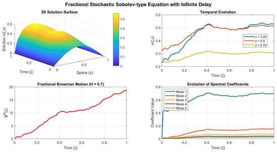
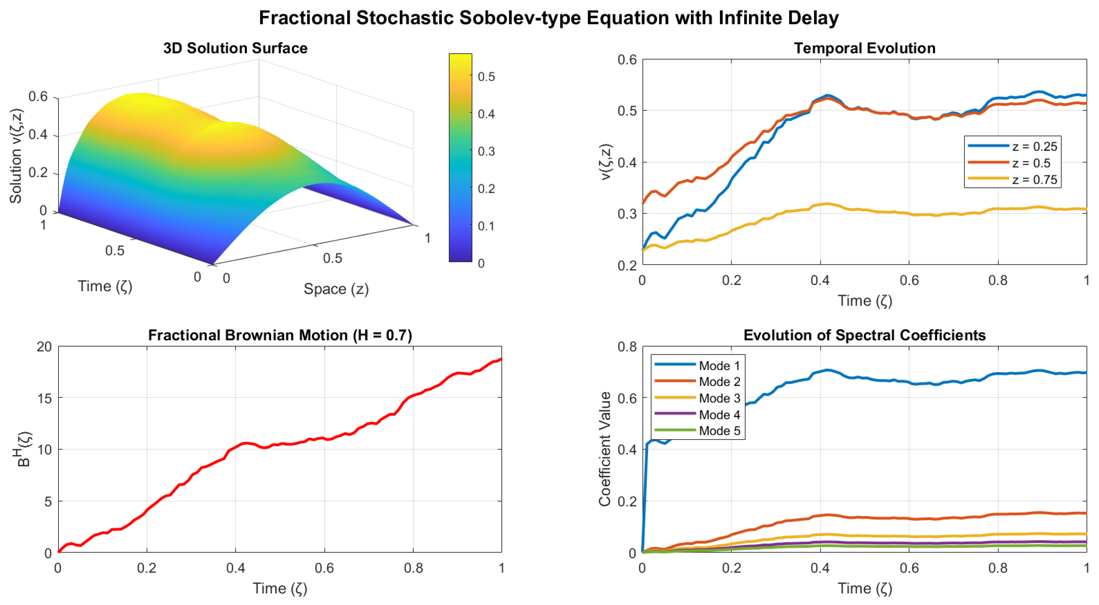
Figure 1 below represents the visual representation of the behavior of the above example.

Figure 1. Fractional Stochastic Sobolev-type Equation with Infinite Delay Visualization via Graph.

The numerical solutions offer a qualitative verification of the theoretical findings proved in Theorem 3. The solution surface in three dimensions illustrates the combined spatiotemporal behavior of the state function $v(\zeta ,z)$ in the region $[0,1]\times [0,1]$. The findings reveal that the solution is bounded and has smooth spatial regularity, thus, verifying the well-posedness of the Sobolev-type problem and the compactness property of ${\mathcal{L}}^{-1}$. Additionally, the temporal responses at specific spatial locations $(z=0.25,0.5,0.75)$ demonstrate convergence to stable trajectories despite the stochastic excitation, indicating that the control component successfully stabilizes the dynamics of the system.

The sample path of the fractional Brownian motion with Hurst parameter H = 0.7 shows the characteristic of long-range dependence and persistence, as expected by the theoretical properties of fBm. Despite the stochastic forcing that causes fluctuations in the system, the solution shows regular growth and does not exhibit instability, which shows the robustness of the approximate controllability result.

Furthermore, the results of the spectral coefficients show that the dynamics are mainly controlled by the lower modes, while the higher modes decay faster due to the semigroup generated by $\mathcal{A}{\mathcal{L}}^{-1}$. The decay rates are in agreement with the compactness and smoothing properties of the semigroup $S\left(\zeta \right)$ and form the basis of the stabilization phenomenon on the solution surface. Therefore, the dominance of the first few modes further supports the approximate controllability of the system.

Overall, the numerical results are in agreement with the analytical solution and show that the proposed Sobolev-type fractional stochastic system with infinite delay is approximately controllable on $[0,1].$

Example 2.

In modern digital signal processing, digital filters are a basic tool for signal manipulation and analysis. They find applications in telecommunication networks, high-end audio processing systems, and medical imaging systems. Digital filters provide accurate spectral processing, which helps in noise reduction, signal smoothing, and the identification of useful spectral information. Digital filters have better flexibility and accuracy than their analog counterparts because they are implemented using algorithms that can be easily modified or optimized. This makes them suitable for the implementation of complex processing algorithms and their ability to keep pace with technological advancements. Digital filters are, therefore, a basic tool in both theoretical and practical developments in DSP. Filters can be generally classified into signal separation and signal restoration operations. Signal separation is a critical operation in the identification of useful information in noisy signals.

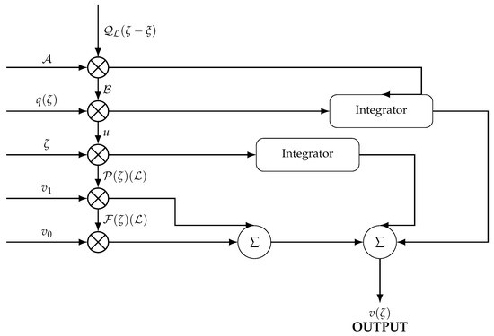
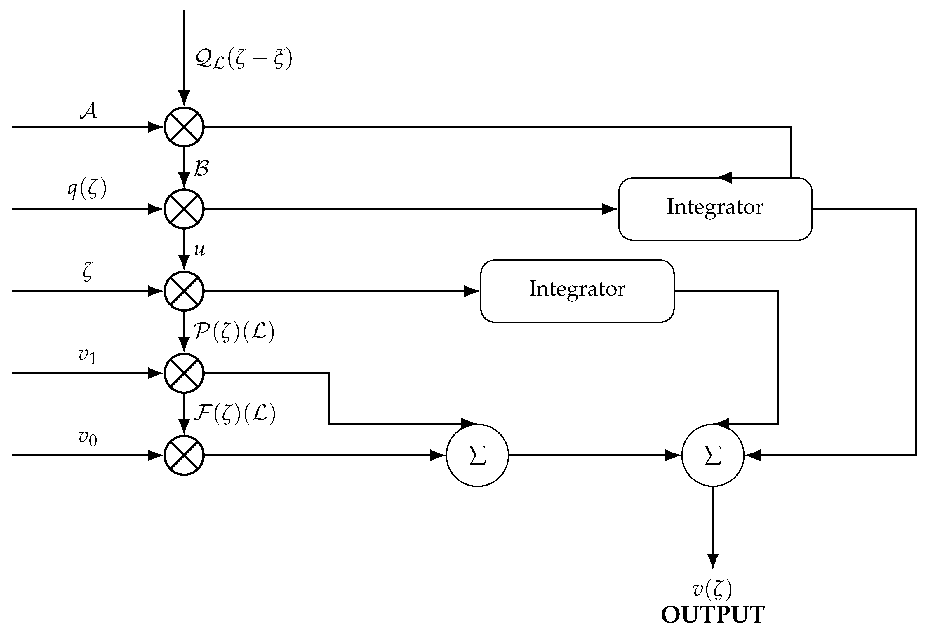
Signal restoration is used to reverse the distortion or modification of a signal due to technological limitations or environmental factors. In real-world applications, such as audio processing, improving recordings made using substandard equipment can be achieved by identifying relevant parts of the signal and rebuilding the original signal structure. Another feasible method would be to establish recursive advanced channels, where each successive output is generated using convolution modeling approaches along with corresponding balancing factors. Based on the approaches outlined in [31,32,33,34], we designed a filter pattern specific to the proposed system, as shown in Figure 2. The block diagram shown in Figure 2 highlights the system design and helps in achieving efficient solutions with simpler inputs.

Figure 2. Filter system for fractional differential system of order $1<\varrho <2$.

The expressions for the terms ${\mathcal{Q}}_{\mathcal{L}}(\zeta -\xi )$ and $\mathcal{B}q\left(\zeta \right)$ are integrated through an appropriate combination. Simultaneously, the expressions for the terms ${\mathcal{Q}}_{\mathcal{L}}(\zeta -\xi )$ and $u\left(\zeta \right)$ undergo the same process of integration. The results obtained from the process of integration for the expressions of the terms are combined in the summation network to obtain a finite pair of optimal control for the state function $v\left(\zeta \right)$ in system (1).

The block diagram, as shown in Figure 2, shows a filter system that is designed to facilitate effective signal processing with a smaller set of input variables. The operations can be summarized as follows:

1. 

Product Modulator-1: Takes inputs A and ${\mathcal{Q}}_{\mathcal{L}}(\zeta -\xi )$, produces the output $A{\mathcal{Q}}_{\mathcal{L}}(\zeta -\xi )$.

2. 

Product Modulator-2: Takes input $\mathcal{B}$ and $q\left(\zeta \right)$, produces the output $\mathcal{B}q\left(\zeta \right)$.

3. 

Product Modulator-3: Takes inputs u and ζ produces directly $u\left(\zeta \right)$.

4. 

Product Modulator-4: At time $t=0$, takes input $v_1$ with $\mathcal{P}\left(\zeta \right)\left(\mathcal{L}\right)$, and produces outputs $\mathcal{P}\left(\zeta \right)\left(\mathcal{L}\right)v_1$.

5. 

Product Modulator-5: Takes $v_0$ with $\mathcal{F}\left(\zeta \right)\left(\mathcal{L}\right)$, produces output $\mathcal{F}\left(\zeta \right)\left(\mathcal{L}{v}_0\right)$.

6. 

Integrators: Evaluates the convolution of ${\mathcal{Q}}_{\mathcal{L}}(\zeta -\xi )$ with $\left[u\right(\zeta )+\mathcal{B}q(\zeta \left)\right]$, thereby contributing to the overall system response.

5. Conclusions

In this paper, we have studied the approximate controllability and existence of solutions for a class of Sobolev-type fractional stochastic differential equations driven by cylindrical fractional Brownian motion. By using the tools of fractional calculus, fixed point theory, and compactness arguments, we have shown the existence of mild solutions and obtained sufficient conditions for approximate controllability. The results obtained here emphasize that the approximate controllability property is retained even in the presence of higher-order fractional derivatives and fractional Brownian motion. This generalizes the classical controllability theory to systems with memory and long-range dependence. The infinite delay and Sobolev-type fractional differential equations increased the complexity of the analysis, which was overcome by using spectral decomposition and semigroup theory in infinite-dimensional Hilbert spaces. Moreover, an example was provided to illustrate the validity and applicability of the theoretical results. An interesting direction for future research is to explore whether Theorems 2 and 3 can be generalized to fractional orders beyond the ranges $(0,1)$ and $(1,2)$. Another interesting area of research would be to explore the controllability conclusions for different fractional derivatives, such as the Hilfer derivative, the Atangana–Baleanu derivative, the Caputo–Fabrizio derivative, and the Hadamard fractional operators. These operators have non-singular or nonlocal kernels, which have a significant effect on the mild solution and may require different fixed point techniques. Further, it would be interesting to consider additional control constraints, including nonlocal conditions, state-dependent delays, impulsive controls, or bounded control functions. The inclusion of such constraints may make the model more realistic in applications but would also pose significant analytical challenges in proving exact or approximate controllability. Finally, generalizing the current framework to systems driven by more general stochastic processes, fractional evolution inclusions, or neutral-type systems may provide further insight into the interplay between control mechanisms, randomness, or memory effects.

References

- Mahmudov, N.I. Approximate controllability of semilinear deterministic and stochastic evolution equations in abstract spaces. Siam J. Control Optim. 2003, 42, 1604–1622. [Google Scholar] [CrossRef] [Scilit]
- Sakthivel, R.; Ganesh, R.; Suganya, S. Approximate controllability of fractional neutral stochastic system with infinite delay. Rep. Math. Phys. 2012, 70, 291–311. [Google Scholar] [CrossRef] [Scilit]
- Gorniewicz, L.; Ntouyas, S.K.; O’Regan, D. Existence and controllability results for first and second order functional semilinear differential inclusions with nonlocal conditions. Numer. Funct. Anal. Optim. 2007, 28, 53–82. [Google Scholar] [CrossRef] [Scilit]
- Agarwal, R.P.; Baghli, S.; Benchohra, M. Controllability for semilinear functional and neutral functional evolution equations with infinite delay in Fréchet spaces. Appl. Math. Optim. 2009, 60, 253–274. [Google Scholar] [CrossRef] [Scilit]
- Benchohra, M.; Ouahab, A. Controllability results for functional semilinear differential inclusions in Fréchet spaces. Nonlinear Anal. Theory Methods Appl. 2005, 61, 405–423. [Google Scholar] [CrossRef] [Scilit]
- Dauer, J.P.; Mahmudov, N.I. Controllability of stochastic semilinear functional differential equations in Hilbert spaces. J. Math. Anal. Appl. 2004, 290, 373–394. [Google Scholar] [CrossRef] [Scilit]
- Kavitha, K.; Vijiyakumar, V.; Udhayakumar, R. Results on controllability of Hilfer fractional neutral differential equations with infinite delay via measures of noncompactness. Chaos Solitons Fractals 2020, 139, 110299. [Google Scholar] [CrossRef] [Scilit]
- Zhou, Y.; He, J.W. New results on controllability of fractional evolution systems with order α∈(1,2). Evol. Equ. Control Theory 2021, 10, 491–509. [Google Scholar] [CrossRef] [Scilit]
- Liu, Z.; Li, X.W. Approximate controllability for a class of hemivariational inequalities. Nonlinear Anal. Theory Methods Appl. 2015, 122, 581–591. [Google Scholar] [CrossRef] [Scilit]
- Lu, L.; Liu, Z.; Bin, M. Approximate controllability for stochastic evolution inclusion of Clarke’s subdifferential type. Appl. Math. Comput. 2016, 286, 201–212. [Google Scholar] [CrossRef] [Scilit]
- Mahmudov, N.I.; Denker, A. On controllability of linear stochastic systems. Int. J. Control 2000, 73, 144–151. [Google Scholar] [CrossRef] [Scilit]
- Mahmudov, N.I.; Udhayakumar, R.; Vijayakumar, V. On the approximate controllability of second-order evolution hemivariational inequalities. Results Math. 2020, 75, 1–19. [Google Scholar] [CrossRef] [Scilit]
- Duncan, T.E.; Pasik-Duncan, B.; Maslowski, B. Fractional Brownian motion and stochastic equations in Hilbert spaces. Stoch. Dyn. 2002, 2, 225–250. [Google Scholar] [CrossRef] [Scilit]
- Biagini, F.; Hu, Y.; Øksendal, B.; Zhang, T. Stochastic Calculus for Fractional Brownian Motion and Applications; Springer: New York, NY, USA, 2008. [Google Scholar]
- Mishura, Y.S. Stochastic Calculus for Fractional Brownian Motion and Related Processes; Springer: Berlin/Heidelberg, Germany, 2008. [Google Scholar]
- Hussain, S.; Sarwar, M.; Shah, S.K.; Abodayeh, K.; Ansari, K.J.; Promsakon, C.; Sitthiwirattam, T. A study on the controllability of Atangana–Baleanu Caputo fractional neutral differential equations with delay. Chaos Solitons Fractals 2025, 201, 117365. [Google Scholar] [CrossRef] [Scilit]
- Algolam, M.S.; Hussain, S.; Younis, B.A.; Osman, O.; Muflh, B.; Aldwoah, K.; Eljaneid, N. Stability and controllability analysis of stochastic fractional differential equations under integral boundary conditions driven by Rosenblatt process with impulses. Fractal Fract. 2025, 9, 146. [Google Scholar] [CrossRef] [Scilit]
- Hussain, S.; Sarwar, M.; Abodayeh, K.; Promsakon, C.; Sitthiwirattham, T. Controllability of Hilfer fractional neutral impulsive stochastic delayed differential equations with nonlocal conditions. Chaos Solitons Fractals 2024, 183, 114876. [Google Scholar] [CrossRef] [Scilit]
- Hussain, S.; Sarwar, M.; Rahmat, G.; Aydi, H.; De La Sen, M. Mild solutions and controllability of fractional evolution inclusions of Clarke’s subdifferential type with nonlocal conditions in Hilbert spaces. Alex. Eng. J. 2023, 80, 58–73. [Google Scholar] [CrossRef] [Scilit]
- Hussain, S.; Sarwar, M.; Nisar, K.S.; Shah, K. Controllability of fractional differential evolution equation of order γ∈(1,2) with nonlocal conditions. AIMS Math. 2023, 8, 14188–14206. [Google Scholar] [CrossRef] [Scilit]
- Hussain, S.; Sarwar, M.; Mlaiki, N.; Azmi, F. Existence and controllability of fractional semilinear mixed Volterra–Fredholm integro differential equation. Alex. Eng. J. 2023, 73, 259–267. [Google Scholar] [CrossRef] [Scilit]
- Abdeljawad, T. Fractional operators with generalized Mittag–Leffler kernels and their iterated differintegrals. Chaos 2019, 29, 023102. [Google Scholar] [CrossRef] [Scilit]
- Sarwar, M.; Hussain, S.; Abodayeh, K.; Moonsuwan, S.; Sitthiwirattham, T. Controllability of semilinear noninstantaneous impulsive neutral stochastic differential equations via Atangana–Baleanu Caputo fractional derivative. Alex. Eng. J. 2024, 94, 149–158. [Google Scholar] [CrossRef] [Scilit]
- Jarad, F.; Abdeljawad, T.; Baleanu, D. On the generalized fractional derivatives and their Caputo modification. J. Nonlinear Sci. Appl. 2017, 10, 2607–2619. [Google Scholar] [CrossRef] [Scilit]
- Gambo, Y.Y.; Jarad, F.; Baleanu, D.; Abdeljawad, T. On Caputo modification of the Hadamard fractional derivatives. Adv. Differ. Equ. 2014, 2014, 10. [Google Scholar] [CrossRef] [Scilit]
- Feckan, M.; Wang, J.; Zhou, Y. Controllability of fractional functional evolution equations of Sobolev type via characteristic solution operators. J. Optim. Theory Appl. 2013, 156, 79–95. [Google Scholar] [CrossRef] [Scilit]
- Cui, J.; Yan, L. Existence result for fractional neutral stochastic integro-differential equations with infinite delay. J. Phys. A Math. Theor. 2011, 44, 335201. [Google Scholar] [CrossRef] [Scilit]
- Guendouzi, T.; Idrissi, S. Approximate controllability of fractional stochastic functional evolution equations driven by a fractional Brownian motion. Romai J. 2012, 8, 103–117. [Google Scholar]
- Pachpatte, B.G. Applications of the Leray–Schauder alternative to some Volterra integral and integrodifferential equations. Indian J. Pure Appl. Math. 1995, 26, 1161–1168. [Google Scholar]
- Li, Y.; Liu, B. Existence of solution of nonlinear neutral stochastic differential inclusion with infinite delay. Stoch. Anal. Appl. 2007, 25, 397–415. [Google Scholar] [CrossRef] [Scilit]
- Chen, W.; Liu, Y.; Zhao, D. Approximate controllability for a class of stochastic impulsive evolution systems with infinite delay involving the fractional substantial derivative. Chaos Solitons Fractals 2024, 182, 114877. [Google Scholar] [CrossRef] [Scilit]
- Valliammal, N.; Jothimani, K.; Johnson, M.; Panda, S.K.; Vijayakumar, V. Approximate controllability analysis of impulsive neutral functional hemivariational inequalities. Commun. Nonlinear Sci. Numer. Simul. 2023, 127, 107560. [Google Scholar] [CrossRef] [Scilit]
- Chandra, A.; Chattopadhyay, S. Design of hardware efficient FIR filter: A review of the state-of-the-art approaches. Eng. Sci. Technol. Int. J. 2016, 19, 212–226. [Google Scholar] [CrossRef] [Scilit]
- Zahoor, S.; Naseem, S. Design and implementation of an efficient FIR digital filter. Cogent Eng. 2017, 4, 1323373. [Google Scholar] [CrossRef] [Scilit]
Disclaimer/Publisher’s Note: The statements, opinions and data contained in all publications are solely those of the individual author(s) and contributor(s) and not of MDPI and/or the editor(s). MDPI and/or the editor(s) disclaim responsibility for any injury to people or property resulting from any ideas, methods, instructions or products referred to in the content. |
© 2026 by the authors. Licensee MDPI, Basel, Switzerland. This article is an open access article distributed under the terms and conditions of the Creative Commons Attribution (CC BY) license.