Mittag-Leffler Weighted Orthogonal Functions for the ABC Fractional Operator: A Formal Self-Adjointness Construction

Abstract

This work constructs an orthogonal function system on bounded intervals $[0,R]$ associated with the Atangana–Baleanu–Caputo (ABC) fractional derivative for $\alpha \in (1/2,1)$. Starting from a fractional Laguerre-type equation involving the ABC operator, solutions are obtained via a generalized Frobenius method, yielding series representations with characteristic exponent $\alpha -1$. Rather than postulating a weight function by analogy with classical or Caputo settings, the weight is derived directly from the requirement that the underlying fractional operator be formally self-adjoint on a suitable admissible domain. This operator-theoretic approach leads to the explicit Mittag–Leffler weight $w_{\alpha }\left(x\right)=x^{-(2\alpha -1)}{E}_{\alpha }(-x^{\alpha })$, which intrinsically reflects the nonlocal memory structure of the ABC kernel. A similarity transformation removes the universal singular factor and produces regularized eigenfunctions that are continuous on $[0,R]$ and orthogonal in the weighted $L^2$ space. The weight identity and formal self-adjointness are rigorously verified through a right-Volterra uniqueness argument. Numerical experiments confirm orthogonality up to machine precision, demonstrate spectral convergence for a model ABC differential equation, and illustrate consistency with classical Laguerre polynomials in the limit $\alpha \to 1^{-}$. The resulting framework provides a self-consistent orthogonal system suitable for spectral approximations of problems governed by the ABC operator on bounded domains.

1. Introduction

Fractional calculus has evolved from a purely mathematical abstraction into a powerful and versatile framework for modeling complex systems that exhibit memory, hereditary properties [1,2,3,4], and anomalous dynamics—phenomena that often elude classical integer-order derivatives [5,6,7,8]. Unlike classical models which rely on local operators, fractional operators incorporate non-local effects that capture the history or spatial distribution of the system, making them indispensable in fields such as viscoelasticity, anomalous diffusion, control theory, and bioengineering [2,7,9,10]. The specific kernel defining a fractional operator dictates the nature of the memory it describes. Traditional power-law kernels, such as those appearing in the Riemann–Liouville and Caputo derivatives, model fading memory with algebraic decay [5,11]. In contrast, kernels based on the Mittag–Leffler function capture more intricate, non-exponential decay patterns with long-range temporal dependencies, offering greater flexibility in modeling real-world phenomena [11,12,13,14,15].

Among contemporary fractional operators, the Atangana–Baleanu (AB) derivative in the Caputo sense has attracted considerable attention due to its unique combination of a non-singular Mittag–Leffler kernel and physically consistent initial conditions [12,13,14,16,17]. This operator has been successfully applied in diverse areas including chaos theory, heat transfer, biological systems, and fractional variational problems [9,14,16]. Unlike the Caputo–Fabrizio derivative, which employs an exponential kernel, the AB derivative retains the Mittag–Leffler function in its definition, thereby preserving the genuinely fractional character of the operator while avoiding the power-law singular kernel present in classical Caputo derivatives [12,13]. This property makes the AB derivative particularly attractive for modeling processes where the kernel should remain bounded yet retain long-range memory effects.

Orthogonal polynomials and special functions form the cornerstone of spectral methods for solving differential equations [18,19]. Among these, classical Laguerre polynomials, orthogonal with respect to the weight $e^{-x}$ on the interval $[0,\infty )$, play a fundamental role in quantum mechanics [20], approximation theory, and numerical analysis [21,22,23,24]. Their spectral convergence properties make them an ideal choice for polynomial approximations on unbounded domains. Extending these classical tools into the fractional domain has been an active area of research over the past two decades [22,25,26]. Notable contributions include the construction of fractional Laguerre functions via the Caputo derivative by Abuasbeh et al. [27], who identified a weight function of the form $w_{\alpha }\left(x\right)=x^{-(2\alpha -1)}{e}^{-x}$ that ensures orthogonality and reduces to the classical case in the appropriate integer-order limit. This work, together with broader investigations into fractional and discrete orthogonal polynomial systems [26,28,29], has laid the groundwork for spectral methods applied to fractional differential equations.

The mathematical challenge becomes significantly deeper when moving from power-law kernels to the non-power-law kernel of the Atangana–Baleanu operator [12,14,16]. The inherent non-locality embedded in the Mittag–Leffler kernel significantly alters the spectral framework applicable to Caputo-type operators [30,31]. Unlike the Caputo case, where the orthogonality structure can often be inferred by analogy with classical polynomial systems, the ABC operator demands a fresh operator-theoretic approach. This raises several fundamental questions: Can an orthogonal system intrinsically adapted to the ABC operator be constructed? What orthogonality structure emerges when the defining memory kernel must be directly reflected in the spectral weight? How does the weight function arise naturally from the operator’s properties rather than being imposed a priori? Resolving these questions is not merely of theoretical interest; it is essential for advancing numerical methods in fractional calculus [7,8,17,32,33] and for applications in fields such as fractional quantum mechanics [34], anomalous diffusion [2], and complex biological systems [9,35].

Recent literature demonstrates growing and diverse interest in fractional Laguerre-type functions and their applications. These range from the numerical solution of fractional Bloch equations in magnetic resonance imaging [36], to bioinformatics applications incorporating fractional memory effects for gene selection [35], and efficient numerical schemes for space-fractional diffusion equations [24,37]. Research has also expanded into generalized and q-analogue forms, such as Mittag–Leffler–Laguerre polynomials [38,39], with connections to fractional optics and beam propagation [40]. Parallel efforts are extending related operator-theoretic constructions to other polynomial bases involving the ABC derivative [41]. This expanding body of work underscores the need for a rigorous and systematic spectral framework tailored specifically to the ABC operator [16,17].

In this paper, we provide a systematic and principle-driven construction of an orthogonal function system intrinsically associated with the Atangana–Baleanu–Caputo fractional derivative. The key novelty lies in deriving the orthogonality structure directly from operator-theoretic considerations rather than postulating a weight function by analogy with classical or Caputo-based constructions. This perspective leads naturally to a Mittag-Leffler weight of the form

$$w_{\alpha }\left(x\right)\propto x^{-(2\alpha -1)}{E}_{\alpha }(-x^{\alpha }),$$

which intrinsically links the polynomial basis to the memory kernel of the ABC operator. To the best of our knowledge, this is among the first constructions in the ABC setting where the orthogonality structure emerges directly from the properties of the operator itself. The main contributions include establishing the formal self-adjointness of the ABC operator on a suitable admissible domain and deriving the associated Mittag–Leffler weight function from first principles. Using a generalized Frobenius method adapted to the nonlocal ABC operator, we construct regularized eigenfunctions that are continuous on bounded intervals $[0,R]$ and satisfy a fractional Laguerre-type equation. Through a similarity transformation, we remove the universal singular factor $x^{\alpha -1}$ and prove orthogonality of the regularized functions in the corresponding weighted $L^2$ space. The theoretical developments are complemented by systematic numerical experiments that confirm orthogonality up to machine precision, demonstrate spectral convergence for a model ABC differential equation, and illustrate consistency with classical Laguerre polynomials in the limit $\alpha \to 1^{-}$. The resulting framework provides a self-consistent orthogonal system suitable for spectral approximations of problems involving the ABC operator on bounded intervals, with the weight function emerging naturally from the operator structure.

The work is structured as follows. Section 2 presents the ABC fractional framework and constructs the ABC–Laguerre functions. Section 2.1 introduces the Atangana–Baleanu–Caputo derivative. Section 2.2 formulates and solves the fractional Laguerre-type equation via a generalized series expansion. Section 2.3 provides the series representation and discusses structural properties of the resulting functions. Section 2.4 establishes the formal self-adjointness of the ABC operator. Section 2.5 derives the associated Mittag–Leffler weight function from first principles. Section 2.6 presents the orthogonality proof via similarity transformation and addresses normalization. Section 3 provides numerical verification and illustrative applications. Section 3.1 validates the orthogonality relations numerically. Section 3.2 presents a spectral method application for solving an ABC differential equation. Section 3.3 discusses numerical accuracy and implementation aspects. Section 3.4 offers concluding remarks and outlines open problems, including extensions to half-line domains, completeness analysis, and asymptotic behavior of normalization constants. Appendix A provides a rigorous verification of the weight function via a right-Volterra uniqueness argument, independent of termwise coefficient matching.

2. The ABC Fractional Framework and Function Construction

2.1. The Atangana–Baleanu–Caputo Derivative

We begin by recalling the definition of the Atangana–Baleanu fractional derivative in the Caputo sense (ABC), which forms the cornerstone of our analysis. For a function $f\in AC[0,b]$, where $AC[0,b]$ denotes the space of absolutely continuous functions on $[0,b]$, the ABC derivative of order $\alpha \in (0,1)$ is defined as

$${}^{ABC}D_{0^{+}}^{\alpha }f\left(x\right)={\displaystyle \frac{B\left(\alpha \right)}{1-\alpha }}{\int }_0^x{f}^{\prime }\left(t\right)E_{\alpha }\left(-{\displaystyle \frac{\alpha }{1-\alpha }}{(x-t)}^{\alpha }\right)dt,$$

(1)

where $B\left(\alpha \right)$ is a normalization function satisfying $B\left(0\right)=B\left(1\right)=1$, and $E_{\alpha }\left(z\right)$ denotes the one-parameter Mittag-Leffler function defined by

$$E_{\alpha }\left(z\right)=\sum _{k=0}^{\infty }{\displaystyle \frac{z^k}{\Gamma (\alpha k+1)}}.$$

(2)

The function $B\left(\alpha \right)$ is a normalization function satisfying $B\left(0\right)=B\left(1\right)=1$; its specific form does not affect the orthogonality structure developed in later sections and may be chosen conveniently (e.g., $B\left(\alpha \right)=1$ or the standard choice $B\left(\alpha \right)=1-\alpha +\alpha /\Gamma \left(\alpha \right)$).

Throughout this work, we focus exclusively on fractional orders $0<\alpha <1$, which corresponds to the standard and well-established definition of the ABC derivative in the literature. This restriction ensures mathematical consistency while maintaining the essential non-local characteristics of the operator that are crucial for our spectral analysis.

A fundamental property of the ABC derivative is its action on power functions, which is essential for the series solution method we will employ. The following lemma provides this result in a rigorous form.

Lemma 1 

(ABC derivative of power functions). For $\mu >-1$ and $\alpha \in (0,1)$, the ABC derivative of $x^{\mu }$ is given by

$${}^{ABC}D_{0^{+}}^{\alpha }{x}^{\mu }={\displaystyle \frac{B\left(\alpha \right)}{1-\alpha }}\sum _{m=0}^{\infty }{\displaystyle \frac{{\left(-\frac{\alpha }{1-\alpha }\right)}^m}{\Gamma (\alpha m+1)}}{\displaystyle \frac{\Gamma (\mu +1)}{\Gamma (\mu +\alpha m+1)}}{x}^{\mu +\alpha m},$$

(3)

where the series converges absolutely for all $x\ge 0$.

Proof. 

Starting from the definition (1), we have

$${}^{ABC}D_{0^{+}}^{\alpha }{x}^{\mu }={\displaystyle \frac{B\left(\alpha \right)}{1-\alpha }}{\int }_0^x\mu t^{\mu -1}{E}_{\alpha }\left(-{\displaystyle \frac{\alpha }{1-\alpha }}{(x-t)}^{\alpha }\right)dt.$$

Substituting the series representation of the Mittag–Leffler function (2) into the integral yields

$${}^{ABC}D_{0^{+}}^{\alpha }{x}^{\mu }={\displaystyle \frac{B\left(\alpha \right)}{1-\alpha }}\sum _{m=0}^{\infty }{\displaystyle \frac{{\left(-\frac{\alpha }{1-\alpha }\right)}^m}{\Gamma (\alpha m+1)}}{\int }_0^x\mu t^{\mu -1}{(x-t)}^{\alpha m}dt.$$

The integral can be evaluated using the Beta function identity:

$${\int }_0^x{t}^{\mu -1}{(x-t)}^{\alpha m}dt=x^{\mu +\alpha m}{\displaystyle \frac{\Gamma \left(\mu \right)\Gamma (\alpha m+1)}{\Gamma (\mu +\alpha m+1)}}.$$

Substituting this result and simplifying using the Gamma function property $\Gamma (\mu +1)=\mu \Gamma \left(\mu \right)$ gives

$${}^{ABC}D_{0^{+}}^{\alpha }{x}^{\mu }={\displaystyle \frac{B\left(\alpha \right)}{1-\alpha }}\sum _{m=0}^{\infty }{\displaystyle \frac{{\left(-\frac{\alpha }{1-\alpha }\right)}^m}{\Gamma (\alpha m+1)}}{\displaystyle \frac{\Gamma (\mu +1)}{\Gamma (\mu +\alpha m+1)}}{x}^{\mu +\alpha m}.$$

The condition $\mu >-1$ ensures the convergence of the Beta integral and guarantees that $\Gamma \left(\mu \right)$ is finite; the case $\mu =0$ is handled by interpreting the product $\mu \Gamma \left(\mu \right)$ as $\Gamma (\mu +1)=1$. The absolute convergence of the resulting series follows from the analytic properties of the Mittag-Leffler function for $\alpha \in (0,1)$.  □

This series representation is fundamental as it allows us to compute the action of the ABC derivative on power series solutions, which will be our primary tool in solving the fractional Laguerre-type equation. The form (3) explicitly shows how the non-local Mittag–Leffler kernel modifies the classical fractional derivative of power functions through an infinite series of fractional power terms.

2.2. Fractional Laguerre-Type Equation and Series Solution

We define the fractional Laguerre-type equation involving the Atangana–Baleanu–Caputo (ABC) derivative and the Atangana–Baleanu (AB) fractional integral by

$$x{}^{ABC}D_{0^{+}}^{\alpha }y\left(x\right)+(1-x){}^{AB}I_{0^{+}}^{1-\alpha }y\left(x\right)+ny\left(x\right)=0,n\in {\mathbb{N}}_0,\alpha \in (0,1).$$

(4)

Equation (4) is understood as a formal spectral problem: we seek functions y (within an admissible class specified in Section 2.4) that satisfy (4) for a given $n\in {\mathbb{N}}_0$. The Frobenius construction below yields formal series solutions indexed by n; their admissibility requirements and numerical stability under truncation are discussed in Section 2.4 and validated in Section 3. A full spectral analysis (discreteness, completeness, etc.) is beyond the scope of this work; the resulting family is primarily used as an orthogonal system for spectral approximations.

The AB fractional integral of order $1-\alpha$ is taken in the standard form

$${}^{AB}I_{0^{+}}^{1-\alpha }f\left(x\right)={\displaystyle \frac{1-\alpha }{B(1-\alpha )}}f\left(x\right)+{\displaystyle \frac{\alpha }{B(1-\alpha )}}{}^{RL}I_{0^{+}}^{1-\alpha }f\left(x\right),$$

(5)

where $B(·)$ is the same normalization function used in the ABC derivative, and ${}^{RL}I_{0^{+}}^{1-\alpha }$ denotes the Riemann–Liouville fractional integral.

To analyze (4), we seek a generalized power-series representation near the origin of the form

$$y\left(x\right)=\sum _{k=0}^{\infty }{a}_k{x}^{k+\beta },a_0\ne 0,\beta >-1,$$

(6)

where $\beta$ will be determined by structural requirements of the equation. The solutions are sought in the class of functions that are absolutely continuous on $(0,R]$ and satisfy boundary conditions at $x=0$ and $x=R$ (to be specified in Section 2.4); the exponent $\beta$ is fixed by consistency with the fractional operator structure.

We first record the action of the AB integral on power functions.

Lemma 2 

(AB integral of power functions). Let $\mu >-1$ and $\alpha \in (0,1)$. Then

$${}^{AB}I_{0^{+}}^{1-\alpha }{x}^{\mu }={\displaystyle \frac{1-\alpha }{B(1-\alpha )}}{x}^{\mu }+{\displaystyle \frac{\alpha }{B(1-\alpha )}}{\displaystyle \frac{\Gamma (\mu +1)}{\Gamma (\mu +2-\alpha )}}{x}^{\mu +1-\alpha }.$$

(7)

Proof. 

The identity follows directly from (5) and the classical formula

$${}^{RL}I_{0^{+}}^{1-\alpha }{x}^{\mu }={\displaystyle \frac{\Gamma (\mu +1)}{\Gamma (\mu +2-\alpha )}}{x}^{\mu +1-\alpha },\mu >-1.$$

□

Applying Lemmas 1 and 2 termwise to (6) yields

$$\begin{array}{cc}\hfill {}^{ABC}D_{0^{+}}^{\alpha }y\left(x\right)& ={\displaystyle \frac{B\left(\alpha \right)}{1-\alpha }}\sum _{k=0}^{\infty }\sum _{m=0}^{\infty }{a}_k{\displaystyle \frac{{\left(-\frac{\alpha }{1-\alpha }\right)}^m}{\Gamma (\alpha m+1)}}{\displaystyle \frac{\Gamma (k+\beta +1)}{\Gamma (k+\beta +\alpha m+1)}}{x}^{k+\beta +\alpha m},\hfill \end{array}$$

(8)

and

$$\begin{array}{cc}\hfill {}^{AB}I_{0^{+}}^{1-\alpha }y\left(x\right)& =\sum _{k=0}^{\infty }{a}_k\left[{\displaystyle \frac{1-\alpha }{B(1-\alpha )}}{x}^{k+\beta }+{\displaystyle \frac{\alpha }{B(1-\alpha )}}{\displaystyle \frac{\Gamma (k+\beta +1)}{\Gamma (k+\beta +2-\alpha )}}{x}^{k+\beta +1-\alpha }\right].\hfill \end{array}$$

(9)

Substituting (6)–(9) into (4) gives the coupled series identity

$$\begin{array}{cc}\hfill & {\displaystyle \frac{B\left(\alpha \right)}{1-\alpha }}\sum _{k=0}^{\infty }\sum _{m=0}^{\infty }{a}_k{\displaystyle \frac{{\left(-\frac{\alpha }{1-\alpha }\right)}^m}{\Gamma (\alpha m+1)}}{\displaystyle \frac{\Gamma (k+\beta +1)}{\Gamma (k+\beta +\alpha m+1)}}{x}^{k+\beta +\alpha m+1}\hfill \\ \hfill & +{\displaystyle \frac{1-\alpha }{B(1-\alpha )}}\sum _{k=0}^{\infty }{a}_k{x}^{k+\beta }-{\displaystyle \frac{1-\alpha }{B(1-\alpha )}}\sum _{k=0}^{\infty }{a}_k{x}^{k+\beta +1}\hfill \\ \hfill & +{\displaystyle \frac{\alpha }{B(1-\alpha )}}\sum _{k=0}^{\infty }{a}_k{\displaystyle \frac{\Gamma (k+\beta +1)}{\Gamma (k+\beta +2-\alpha )}}{x}^{k+\beta +1-\alpha }-{\displaystyle \frac{\alpha }{B(1-\alpha )}}\sum _{k=0}^{\infty }{a}_k{\displaystyle \frac{\Gamma (k+\beta +1)}{\Gamma (k+\beta +2-\alpha )}}{x}^{k+\beta +2-\alpha }\hfill \\ \hfill & +n\sum _{k=0}^{\infty }{a}_k{x}^{k+\beta }=0.\hfill \end{array}$$

(10)

To investigate the behavior near the origin, note that $\alpha \in (0,1)$ implies that all powers generated by the ABC term in (10) are strictly larger than $\beta$. If one attempts a classical Frobenius lowest-power balance, the coefficient of $x^{\beta }$ would formally suggest

$$a_0\left({\displaystyle \frac{1-\alpha }{B(1-\alpha )}}+n\right)=0.$$

(11)

Since (11) depends only on n and $\alpha$, it cannot hold for arbitrary $n\in {\mathbb{N}}_0$, indicating that the standard indicial-equation mechanism is not applicable in the present nonlocal setting. This reflects an intrinsic feature of the ABC operator: the nonlocal Mittag–Leffler kernel induces global coefficient coupling, so that the leading exponent $\beta$ cannot be determined by a simple lowest-power balance, but instead must be fixed by consistency of the full fractional operator structure.

A systematic inspection of the exponents in (10) shows that, for a general $\beta$, the AB-integral term produces powers of the form $x^{k+\beta +1-\alpha }$, which are not aligned with the integer lattice generated by the remaining terms. Requiring a closed and well-ordered exponent structure therefore imposes a structural constraint on $\beta$.

Lemma 3 

(Determination of the Frobenius exponent). Let $\alpha \in (0,1)$. The choice $\beta =\alpha -1$ is the unique one that yields a closed exponent scale for coefficient matching, in the sense that all powers appearing in (10) belong to the ordered family

$${\{x^{k+\alpha -1},x^k,x^{k+1},x^{k+\alpha },x^{k+\alpha +1},\dots \}}_{k\ge 0}.$$

Proof. 

For $\beta =\alpha -1$, the term $x^{k+\beta +1-\alpha }$ reduces to $x^k$, which lies on the integer lattice generated by the remaining contributions in (10). Any other choice of $\beta$ produces an incommensurate fractional shift, preventing closure of the coefficient-matching system.  □

Moreover, the choice $\beta =\alpha -1$ implies the local behavior $y\left(x\right)\sim x^{\alpha -1}$ as $x\to 0^{+}$, which is compatible with admissibility in the weighted space induced by the Mittag–Leffler weight derived in Section 2.8. Thus, $\beta =\alpha -1$ is not merely convenient, but necessary for the formal coefficient-matching framework adopted here.

Setting $\beta =\alpha -1$, the identity (10) can be reorganized by collecting identical powers of x, yielding an infinite linear system of the form

$$\mathcal{A}{\left\{a_k\right\}}_{k\ge 0}=0,$$

(12)

where $\mathcal{A}$ is a linear operator acting on the coefficient sequence ${\left\{a_k\right\}}_{k\ge 0}$. The nonlocal Mittag–Leffler kernel induces global coupling, whereby each coefficient $a_k$ interacts with infinitely many others. Consequently, the resulting system does not reduce to a finite-term recurrence relation, but instead yields an infinite-dimensional linear structure intrinsically determined by the ABC operator.

For computational purposes, we introduce truncated approximations. Let $P_N$ denote the projection onto the finite-dimensional span of ${\left\{x^{k+\alpha -1}\right\}}_{k=0}^N$. The truncated system

$$P_N\mathcal{A}{P}_N{\left\{a_k\right\}}_{k=0}^N=0$$

(13)

yields a finite linear system whose solution defines the truncated fractional Laguerre-type function

$$L_n^{(\alpha ,N)}\left(x\right)=\sum _{k=0}^N{a}_k^{\left(n\right)}{x}^{k+\alpha -1}.$$

(14)

Numerical experiments in Section 3 indicate that, for fixed $\alpha$ and n, the sequence ${\left\{L_n^{(\alpha ,N)}\right\}}_{N\ge 1}$ stabilizes rapidly in the weighted $L^2$-norm induced by the Mittag–Leffler weight, providing effective spectral approximations of solutions to (4).

The admissibility requirements for the infinite-series representation and the behavior of truncated approximations are discussed in Section 2.4 and validated numerically in Section 3. All numerical implementations employ appropriately truncated versions of (6).

2.3. Closed-Form Expression and Structural Properties

Because of the nonlocal structure of the ABC operator and the resulting infinite coupling in the coefficient system (12), a simple closed-form expression in terms of elementary functions does not arise. Instead, the fractional Laguerre-type functions are defined through their truncated series representation (14), with coefficients determined by the projected linear system

$$P_N\mathcal{A}{P}_N{\left\{a_k\right\}}_{k=0}^N=0,$$

(15)

where $\mathcal{A}$ denotes the infinite-dimensional operator acting on the coefficient sequence and $P_N$ is the canonical projection onto the first $N+1$ modes.

We emphasize that the construction is formal at the level of the infinite system, while all computational realizations employ truncated versions. Within this framework, several structural observations follow directly from the series representation developed in Section 2.2.

Property 1 

(Dependence on the fractional parameter). For any fixed truncation order N and fixed $x\in [0,R]$, the truncated function $L_n^{(\alpha ,N)}\left(x\right)$ depends continuously on $\alpha \in (0,1)$. This behavior is consistent with the analytic dependence of the Frobenius coefficients on α in the formal construction. No differentiability statement or classical limiting structure is assumed.

Property 2 

(Growth and weighted square-integrability). For each fixed N, the truncated function

$$L_n^{(\alpha ,N)}\left(x\right)=\sum _{k=0}^N{a}_k^{\left(n\right)}{x}^{k+\alpha -1}$$

exhibits algebraic growth as x increases. However, when combined with the Mittag–Leffler weight

$$w_{\alpha }\left(x\right)=x^{-(2\alpha -1)}{E}_{\alpha }(-x^{\alpha }),$$

derived in Section 2.8, the product $w_{\alpha }\left(x\right)L_n^{(\alpha ,N)}\left(x\right)$ is square-integrable on any fixed bounded interval $[0,R]$. The extension of this property to the half-line $[0,\infty )$ would require additional decay analysis and is not addressed in the present work.

Due to the global coupling induced by the nonlocal Mittag–Leffler kernel, classical structural features of orthogonal polynomial systems—such as a three-term recurrence relation, a Rodrigues formula, or a closed generating function— do not directly carry over to the ABC setting. Instead, the truncated family ${\left\{L_n^{(\alpha ,N)}\right\}}_{n=0}^N$ derives its practical relevance from the orthogonality structure established in Section 2.11 and from its effectiveness in spectral approximation schemes.

The stability and convergence behavior of the truncated systems (15) are examined numerically in Section 3. A rigorous analysis of truncation error and infinite-dimensional solvability remains an open problem.

2.4. Formal Self-Adjointness of the ABC Operator

The orthogonality structure of the fractional Laguerre-type system is derived from the formal self-adjointness of the operator

$$\mathcal{L}\left[y\right]\left(x\right)=x{}^{ABC}D_{0^{+}}^{\alpha }y\left(x\right)+(1-x){}^{AB}I_{0^{+}}^{1-\alpha }y\left(x\right),0<x<R,$$

(16)

defined for $0<\alpha <1$ on a fixed bounded interval $[0,R]$.

2.4.1. Analytical Status of the Construction

In this section we establish formal self-adjointness of $\mathcal{L}$ with respect to a weighted inner product on a specified admissible class of functions. By “formal self-adjointness” we mean that the identity

$${⟨\mathcal{L}\left[f\right],g⟩}_w={⟨f,\mathcal{L}\left[g\right]⟩}_w$$

holds for all admissible functions $f,g$, based on integration-by-parts identities and the vanishing of boundary contributions.

We do not claim that $\mathcal{L}$ defines a closed, densely defined, self-adjoint operator in the Hilbert space $L^2([0,R];wdx)$. No spectral theorem, closedness result, or completeness property is asserted in this work.

2.4.2. Weighted Framework

Let $w:[0,R]\to [0,\infty )$ be a fixed candidate weight. Define the weighted inner product

$${⟨f,g⟩}_w={\int }_0^{R}w\left(x\right)f\left(x\right)g\left(x\right)dx,$$

(17)

whenever the integral converges.

For this fixed weight w, define the admissible domain

$${\mathcal{D}}_{\alpha }\left(w\right):=\left\{f\in AC\left([0,R]\right):{\int }_0^{R}w\left(x\right){\left|f\left(x\right)\right|}^{2}dx<\infty ,\right\}.$$

(18)

and all boundary contributions arising in the weighted integration-by-parts identity vanish.

Here $AC\left(\right[0,R\left]\right)$ denotes the space of absolutely continuous functions on $[0,R]$. In particular, the admissible class is chosen so that all fractional integrals and derivatives appearing in (16) are well-defined almost everywhere on $(0,R)$. All identities below are understood to hold on ${\mathcal{D}}_{\alpha }\left(w\right)$.

Throughout this subsection we write

$$\kappa ={\displaystyle \frac{\alpha }{1-\alpha }}.$$

(19)

2.4.3. Right-Sided Adjoint Operators with Terminal R

From the weighted integration-by-parts identity, the right-sided adjoint of the ABC derivative with terminal R takes the form

$$\left({}^{ABC}\mathcal{D}_{R^{-}}^{\alpha }\varphi \right)\left(t\right)={\displaystyle \frac{B\left(\alpha \right)}{1-\alpha }}\left[\varphi \left(t\right)-\kappa {\int }_t^R\varphi \left(x\right){(x-t)}^{\alpha -1}{E}_{\alpha ,\alpha }\left(-\kappa {(x-t)}^{\alpha }\right)dx\right],$$

(20)

for $0<t<R$.

For the AB integral, we use the decomposition

$${}^{AB}I_{0^{+}}^{1-\alpha }={\displaystyle \frac{1-\alpha }{B(1-\alpha )}}I+{\displaystyle \frac{\alpha }{B(1-\alpha )}}{}^{RL}I_{0^{+}}^{1-\alpha }.$$

(21)

On the bounded interval $[0,R]$, the classical Riemann–Liouville adjoint relation yields

$${\int }_0^R\varphi \left(x\right){}^{RL}I_{0^{+}}^{1-\alpha }\psi \left(x\right)dx={\int }_0^R\psi \left(x\right){}^{RL}I_{R^{-}}^{1-\alpha }\varphi \left(x\right)dx,$$

(22)

for sufficiently regular functions for which the integrals converge and boundary terms vanish; in particular, this holds for functions in the admissible class ${\mathcal{D}}_{\alpha }\left(w\right)$.

Consequently, the right-sided AB adjoint operator with terminal R is

$$\left({}^{AB}I_{R^{-}}^{1-\alpha }\varphi \right)\left(x\right)={\displaystyle \frac{1-\alpha }{B(1-\alpha )}}\varphi \left(x\right)+{\displaystyle \frac{\alpha }{B(1-\alpha )}}{}^{RL}I_{R^{-}}^{1-\alpha }\varphi \left(x\right).$$

(23)

These right-sided operators allow the weighted adjoint identity for $\mathcal{L}$ to be expressed entirely on the bounded interval $[0,R]$. The explicit verification of the formal self-adjointness condition, together with the derivation of the corresponding weight function, is presented in Theorem A2 (Appendix A).

2.5. Formal Adjoint Computation

Lemma 4 

(Differentiation of the right-sided Mittag–Leffler operator). Let $\alpha \in (0,1)$ and let $\varphi \in L^1(0,\infty )$. Define

$$\left({\mathcal{I}}_{\alpha ,\infty }\varphi \right)\left(t\right):={\displaystyle \frac{B\left(\alpha \right)}{1-\alpha }}{\int }_t^{\infty }\varphi \left(x\right)E_{\alpha }(-\kappa {(x-t)}^{\alpha })dx,t>0.$$

Then ${\mathcal{I}}_{\alpha ,\infty }\varphi$ is absolutely continuous on $(0,\infty )$ and for almost every $t>0$,

$${\displaystyle \frac{d}{dt}}\left({\mathcal{I}}_{\alpha ,\infty }\varphi \right)\left(t\right)={\displaystyle \frac{B\left(\alpha \right)}{1-\alpha }}\left[-\varphi \left(t\right)+\kappa {\int }_t^{\infty }\varphi \left(x\right){(x-t)}^{\alpha -1}{E}_{\alpha ,\alpha }(-\kappa {(x-t)}^{\alpha })dx\right].$$

Equivalently,

$${\displaystyle \frac{d}{dt}}\left({\mathcal{I}}_{\alpha ,\infty }\varphi \right)\left(t\right)=-{(}^{ABC}{\mathcal{D}}_{\infty -}^{\alpha }\varphi )\left(t\right).$$

Theorem 1 

(Formal adjoint). For a fixed weight w, the formal adjoint of $\mathcal{L}$ with respect to ${⟨·,·⟩}_w$ is

$${\mathcal{L}}_w^{*}\left[g\right]={}^{ABC}\mathcal{D}_{{\infty }^{-}}^{\alpha }\left(xwg\right)+{}^{AB}I_{{\infty }^{-}}^{1-\alpha }\left((1-x)wg\right).$$

(24)

Proof. 

We compute

$${⟨\mathcal{L}\left[f\right],g⟩}_w=I_1+I_2,$$

where

$$I_1={\int }_0^{\infty }w\left(x\right)g\left(x\right)x{}^{ABC}D_{0^{+}}^{\alpha }f\left(x\right)dx,I_2={\int }_0^{\infty }w\left(x\right)g\left(x\right)(1-x){}^{AB}I_{0^{+}}^{1-\alpha }f\left(x\right)dx.$$

Term I₁.

Applying Lemma 4 with $\phi \left(x\right)=xw\left(x\right)g\left(x\right)$ gives

$$I_1={\int }_0^{\infty }f\left(x\right){}^{ABC}\mathcal{D}_{{\infty }^{-}}^{\alpha }\left(xwg\right)\left(x\right)dx,$$

since boundary terms vanish on ${\mathcal{D}}_{\alpha }\left(w\right)$.

Term I₂.

Using the AB decomposition,

$$I_2={\displaystyle \frac{1-\alpha }{B(1-\alpha )}}{\int }_0^{\infty }w(1-x)gfdx+{\displaystyle \frac{\alpha }{B(1-\alpha )}}{\int }_0^{\infty }w(1-x)g{}^{RL}I_{0^{+}}^{1-\alpha }fdx.$$

Applying (22) to the second integral yields

$$I_2={\int }_0^{\infty }f\left(x\right){}^{AB}I_{{\infty }^{-}}^{1-\alpha }\left((1-x)wg\right)\left(x\right)dx.$$

Combining $I_1$ and $I_2$ gives

$${⟨\mathcal{L}\left[f\right],g⟩}_w={\int }_0^{\infty }f\left(x\right)\left[{}^{ABC}\mathcal{D}_{{\infty }^{-}}^{\alpha }\left(xwg\right)+{}^{AB}I_{{\infty }^{-}}^{1-\alpha }\left((1-x)wg\right)\right]\left(x\right)dx,$$

which proves (24).  □

2.6. Formal Self-Adjointness Condition

We now characterize the weights for which $\mathcal{L}$ is formally self-adjoint with respect to the weighted inner product (17) on the bounded interval $[0,R]$.

Theorem 2 

(Formal self-adjointness condition). Let $w:[0,R]\to [0,\infty )$ be a fixed weight and let ${\mathcal{D}}_{\alpha }\left(w\right)$ be the admissible class defined in Section 2.4. Then $\mathcal{L}$ is formally self-adjoint on ${\mathcal{D}}_{\alpha }\left(w\right)$ (i.e. ${⟨\mathcal{L}\left[f\right],g⟩}_w={⟨f,\mathcal{L}\left[g\right]⟩}_w$ for all $f,g\in {\mathcal{D}}_{\alpha }\left(w\right)$) if and only if

$${\mathcal{L}}_w^{*}\left[g\right]\left(x\right)=w\left(x\right)\mathcal{L}\left[g\right]\left(x\right)\mathit{in}\mathit{the}\mathit{distributional}\mathit{sense}\mathit{on}(0,R),$$

(25)

for all $g\in {\mathcal{D}}_{\alpha }\left(w\right)$, where ${\mathcal{L}}_w^{*}$ is the formal adjoint given in Theorem 1. Equivalently, (25) can be written in expanded form as

$${}^{ABC}\mathcal{D}_{R^{-}}^{\alpha }\left(xw\left(x\right)g\left(x\right)\right)+{}^{AB}I_{R^{-}}^{1-\alpha }\left((1-x)w\left(x\right)g\left(x\right)\right)=w\left(x\right)\left(x{}^{ABC}D_{0^{+}}^{\alpha }g\left(x\right)+(1-x){}^{AB}I_{0^{+}}^{1-\alpha }g\left(x\right)\right),$$

(26)

to be understood on $(0,R)$ under the admissibility assumptions of ${\mathcal{D}}_{\alpha }\left(w\right)$.

Proof. 

By Theorem 1, for all $f,g\in {\mathcal{D}}_{\alpha }\left(w\right)$ we have

$${⟨\mathcal{L}\left[f\right],g⟩}_w={\int }_0^{R}f\left(x\right){\mathcal{L}}_w^{*}\left[g\right]\left(x\right)dx,{⟨f,\mathcal{L}\left[g\right]⟩}_w={\int }_0^{R}f\left(x\right)w\left(x\right)\mathcal{L}\left[g\right]\left(x\right)dx.$$

Hence ${⟨\mathcal{L}\left[f\right],g⟩}_w={⟨f,\mathcal{L}\left[g\right]⟩}_w$ for all admissible $f,g$ holds if and only if

$${\int }_0^{R}f\left(x\right)\left({\mathcal{L}}_w^{*}\left[g\right]\left(x\right)-w\left(x\right)\mathcal{L}\left[g\right]\left(x\right)\right)dx=0\mathrm{for}\mathrm{all}f\in {\mathcal{D}}_{\alpha }\left(w\right),$$

which is precisely the distributional identity (25) on $(0,R)$, since the equality holds against all admissible test functions. The expanded form (26) follows by substituting the expressions of $\mathcal{L}$ (16) and ${\mathcal{L}}_w^{*}$ (25).  □

The explicit verification that the Mittag–Leffler weight $w_{\alpha }$ derived in the next subsection satisfies (25) is carried out in Appendix A using the Volterra structure of the right-sided operators.

2.7. Determination of the Weight

Condition (25) is a nonlocal operator constraint on the unknown weight w. Evaluating both sides on the monomial family ${\{g\left(x\right)=x^k\}}_{k\ge 0}$ and using the power-action formulas from Lemmas 1 and 2, together with the right-sided operators defined in Section 2.4, leads to a candidate weight of the form

$$w_{\alpha }\left(x\right)=C{x}^{-(2\alpha -1)}{E}_{\alpha }(-x^{\alpha }),C>0,x\in (0,R),$$

(27)

where $E_{\alpha }$ is the one-parameter Mittag–Leffler function (2). The factor $x^{-(2\alpha -1)}$ compensates the singular behavior $x^{\alpha -1}$ of the Frobenius solutions near $x=0$, while the Mittag–Leffler factor $E_{\alpha }(-x^{\alpha })$ is precisely tuned to cancel the series generated by the right-sided ABC adjoint operator.

The constant C plays no role in the formal symmetry, as it cancels in the weighted inner product; it may therefore be set to $C=1$ for convenience in numerical implementations.

The rigorous verification that (27) satisfies the formal self-adjointness identity (25) is carried out in Appendix A. The proof avoids termwise coefficient matching on $[0,R]$; instead, it uses a right-Volterra integral equation and a uniqueness argument for homogeneous Volterra equations. The main steps are as follows:

• Defining the error functional $F_g\left(x\right)$ as the difference between the left and right sides of (26) applied to g;
• Showing that $F_g$ satisfies a homogeneous right-Volterra equation $F_g=\mathcal{V}{F}_g$ on $[0,R]$;
• Proving that the only continuous solution of $F_g=\mathcal{V}{F}_g$ is $F_g\equiv 0$;
• Concluding that (27) indeed yields formal self-adjointness.

This approach, detailed in Appendix A, provides a complete and rigorous validation of the weight (27) without relying on termwise algebraic manipulations.

2.8. Admissibility and Analytical Properties of the Weight

We now examine the analytical properties of the candidate weight (27) and justify the parameter restrictions under which the weighted framework is well defined.

Throughout this subsection $0<\alpha <1$ and

$$\kappa ={\displaystyle \frac{\alpha }{1-\alpha }}.$$

The normalization function $B(·)$ appearing in the ABC derivative and AB integral satisfies $B\left(0\right)=B\left(1\right)=1$ (see Section 2.1).

2.8.1. Behavior near the Origin and the Restriction $\alpha >\frac{1}{2}$

Since $E_{\alpha }\left(0\right)=1$, the weight

$$w_{\alpha }\left(x\right)=C{x}^{-(2\alpha -1)}{E}_{\alpha }(-x^{\alpha })$$

satisfies

$$w_{\alpha }\left(x\right)\sim C{x}^{-(2\alpha -1)}\mathrm{as}x\to 0^{+}.$$

Hence $w_{\alpha }\in L^1(0,R)$ if and only if

$$-(2\alpha -1)>-1,\mathrm{i}.\mathrm{e}.,\alpha >\frac{1}{2}.$$

Accordingly, in the orthogonality framework developed below we restrict to

$$\alpha \in \left(\frac{1}{2},1\right),$$

(28)

so that the weighted inner product (17) is well defined on $[0,R]$.

2.8.2. Bounded-Interval Formulation

For $0<\alpha <1$, the Mittag–Leffler function $E_{\alpha }(-x^{\alpha })$ decays algebraically as x increases. To avoid additional boundary considerations and to keep the formal integration-by-parts identities within a controlled weighted framework, we develop the orthogonality theory on a fixed bounded interval $[0,R]$ with $R<\infty$.

As in Section 2.4, all right-sided operators are understood with terminal point R. All identities are understood in the distributional sense on $(0,R)$ and, for $\alpha >\frac{1}{2}$, also hold pointwise almost everywhere for functions in the admissible class ${\mathcal{D}}_{\alpha }\left(w\right)$.

2.8.3. Verification of the Formal Self-Adjointness Identity

The verification that the weight (27) satisfies the formal self-adjointness identity (25) is presented in Appendix A, based on the Volterra-type structure induced by the right-sided operators on $[0,R]$.

2.9. Right-Sided Operators with Terminal R

For completeness, we record here the explicit definitions of the right-sided operators with terminal point R, as introduced in Section 2.4. These operators will be used throughout the remainder of the paper and in Appendix A. Recall that the normalization function $B(·)$ satisfies $B\left(0\right)=B\left(1\right)=1$ (see Section 2.1).

We first define the right-sided Riemann–Liouville fractional integral on $(0,R)$:

$$\left({}^{RL}I_{R^{-}}^{\beta }\varphi \right)\left(x\right):={\displaystyle \frac{1}{\Gamma \left(\beta \right)}}{\int }_x^R{(t-x)}^{\beta -1}\varphi \left(t\right)dt,\beta >0,0<x<R,$$

(29)

whenever the integral is well defined.

The right-sided AB fractional integral with terminal R is defined by the standard AB decomposition using the same normalization function $B(·)$:

$$\left({}^{AB}I_{R^{-}}^{1-\alpha }\varphi \right)\left(x\right):={\displaystyle \frac{1-\alpha }{B(1-\alpha )}}\varphi \left(x\right)+{\displaystyle \frac{\alpha }{B(1-\alpha )}}\left({}^{RL}I_{R^{-}}^{1-\alpha }\varphi \right)\left(x\right),0<x<R.$$

(30)

Next, we recall the right-sided Mittag–Leffler averaging operator from Section 2.4, now with terminal R:

$$\left({\mathcal{J}}_{\alpha ,R}\phi \right)\left(t\right):={\displaystyle \frac{B\left(\alpha \right)}{1-\alpha }}{\int }_t^R\phi \left(x\right)E_{\alpha }\left(-\kappa {(x-t)}^{\alpha }\right)dx,0<t<R,$$

(31)

where $\kappa ={\displaystyle \frac{\alpha }{1-\alpha }}$. The integral is well defined whenever the integrand is absolutely integrable on $(t,R)$; in particular, this holds for admissible functions with sufficient local integrability.

Motivated by the integration-by-parts identity, we define the right-sided adjoint ABC operator on $(0,R)$ by

$$\left({}^{ABC}\mathcal{D}_{R^{-}}^{\alpha }\phi \right)\left(t\right):={\displaystyle \frac{B\left(\alpha \right)}{1-\alpha }}\left[\phi \left(t\right)-\kappa {\int }_t^R\phi \left(x\right){(x-t)}^{\alpha -1}{E}_{\alpha ,\alpha }\left(-\kappa {(x-t)}^{\alpha }\right)dx\right],0<t<R,$$

(32)

whenever the integral is well defined. As above, the operator is defined for functions for which the integral term is absolutely integrable on $(t,R)$.

These right-sided operators play a central role in the weighted integration-by-parts identities and in the verification of the formal self-adjointness condition presented in Appendix A.

2.10. Target Identity and Verification on $(0,R)$

By Theorem 2 (with the terminal point fixed at R), formal self-adjointness of $\mathcal{L}$ with respect to the weighted inner product

$${⟨f,g⟩}_w:={\int }_0^{R}w\left(x\right)f\left(x\right)g\left(x\right)dx$$

(33)

is equivalent to the distributional identity

$${}^{ABC}\mathcal{D}_{R^{-}}^{\alpha }\left(xw\left(x\right)g\left(x\right)\right)+{}^{AB}I_{R^{-}}^{1-\alpha }\left((1-x)w\left(x\right)g\left(x\right)\right)=w\left(x\right)\mathcal{L}\left[g\right]\left(x\right)\mathrm{in}{\mathcal{D}}^{\prime }(0,R),$$

(34)

for all admissible test functions g (in particular, for all polynomials), where the right-sided operators are those recorded in Section 2.9.

2.10.1. Auxiliary Finite-Terminal Identities

Lemma 5 

(Right-sided AB integral on powers). Let $0<\alpha <1$ and $k\in {\mathbb{N}}_0$. Then for $0<x<R$,

$$\left({}^{AB}I_{R^{-}}^{1-\alpha }{x}^k\right)\left(x\right)={\displaystyle \frac{1-\alpha }{B(1-\alpha )}}{x}^k+{\displaystyle \frac{\alpha }{B(1-\alpha )}}{\displaystyle \frac{1}{\Gamma (1-\alpha )}}{\int }_x^R{(t-x)}^{-\alpha }{t}^{k}dt,$$

(35)

and the integral is finite for each $x\in (0,R)$.

Proof. 

This follows directly from the AB decomposition (30) and the definition of the right-sided Riemann–Liouville integral (29). The kernel ${(t-x)}^{-\alpha }$ is integrable near $t=x$ since $-\alpha >-1$.  □

Lemma 6 

(Finite-terminal Mittag–Leffler differentiation). Fix $0<\alpha <1$ and let $\kappa ={\displaystyle \frac{\alpha }{1-\alpha }}$. Let $\phi \in L^1(0,R)$ be such that

$${\int }_t^R\left|\phi \left(x\right)\right|{(x-t)}^{\alpha -1}dx<\infty \mathit{for}a.e.t\in (0,R)$$

(this holds, in particular, for functions in the admissible class ${\mathcal{D}}_{\alpha }\left(w\right)$). Then the operator ${\mathcal{J}}_{\alpha ,R}$ defined in (31) is absolutely continuous on $(0,R)$ and satisfies

$${\displaystyle \frac{d}{dt}}\left({\mathcal{J}}_{\alpha ,R}\phi \right)\left(t\right)=-\left({}^{ABC}\mathcal{D}_{R^{-}}^{\alpha }\phi \right)\left(t\right)\mathit{for}a.e.t\in (0,R),$$

(36)

where ${}^{ABC}\mathcal{D}_{R^{-}}^{\alpha }$ is given by (32).

Proof. 

This is the finite-terminal analogue of Lemma 5, obtained by the same Leibniz differentiation under the integral sign, with terminal point R. The additional integrability condition ensures that differentiation under the integral sign is justified.  □

2.10.2. Candidate Weight and Formal Verification

Motivated by the Frobenius exponent $\beta =\alpha -1$ in Section 2.2 and the Mittag–Leffler structure of the ABC kernel, we consider the weight

$$w_{\alpha }\left(x\right):=C{x}^{-(2\alpha -1)}{E}_{\alpha }(-x^{\alpha }),0<x\le R,C>0.$$

(37)

For $\alpha \in (\frac{1}{2},1)$ one has $w_{\alpha }\in L^1(0,R)$ and $w_{\alpha }\left(x\right)>0$ on $(0,R]$ (since $E_{\alpha }(-x^{\alpha })>0$ for $x\ge 0$). The constant C plays no role in the formal symmetry and may be set to $C=1$ without loss of generality.

Theorem 3 

(Verification of the weight identity). Let $\alpha \in (\frac{1}{2},1)$ and $R\in (0,\infty )$. Then the weight $w_{\alpha }$ in (27) satisfies (34) for every polynomial g, in the distributional sense on $(0,R)$. Consequently, $\mathcal{L}$ is formally self-adjoint with respect to ${⟨·,·⟩}_{w_{\alpha }}$ on the admissible class ${\mathcal{D}}_{\alpha }\left(w_{\alpha }\right)$.

Proof. 

By linearity, it suffices to verify (34) for monomials $g\left(x\right)=x^k$, $k\in {\mathbb{N}}_0$. For such g, the right-hand side $w_{\alpha }\mathcal{L}\left[g\right]$ is computed using the left-sided power-action formulas from Section 2.2, while the left-hand side is expressed via the finite-terminal identities in Lemmas 5 and 6.

A complete verification is given in Appendix A using a right-Volterra uniqueness argument: the difference between the two sides of (34) is shown to satisfy a homogeneous Volterra-type equation on $(0,R)$, whose only admissible solution is the zero distribution. This establishes (34) on the polynomial class.  □

Remark 1 

(Non-uniqueness). We do not claim uniqueness of the weight. The function $w_{\alpha }$ is one admissible choice that satisfies the formal symmetry identity (34) under the stated assumptions.

2.11. Orthogonality Proof and Normalization

We establish the orthogonality of the ABC–Laguerre family with respect to the weight $w_{\alpha }$ derived in Section 2.8 and introduce a consistent normalization. Throughout this subsection we fix $\alpha \in (1/2,1)$ and a bounded interval $[0,R]$ with $R<\infty$. We assume that the Frobenius series representation (39) for the eigenfunctions converges on $[0,R]$.

2.11.1. Regularized Eigenfunctions

Recall from Section 2.2 that the eigenvalue problem

$$\mathcal{L}\left[y\right]\left(x\right)=-ny\left(x\right),n\in {\mathbb{N}}_0,$$

(38)

admits Frobenius-type solutions of the form

$$y_n\left(x\right)=x^{\alpha -1}\sum _{k=0}^{\infty }{a}_k\left(n\right)x^k,a_0\left(n\right)=1.$$

(39)

Since $w_{\alpha }\left(x\right)\sim C{x}^{-(2\alpha -1)}$ as $x\to 0^{+}$, the integrand $w_{\alpha }\left(x\right)y_n{\left(x\right)}^2$ behaves like $x^{-1}$ near the origin and is therefore not integrable. Thus the weighted $L^2$-orthogonality must be formulated for the regularized eigenfunctions obtained by removing the universal singular factor $x^{\alpha -1}$.

Definition 1 

(Regularized ABC–Laguerre functions). For each $n\in {\mathbb{N}}_0$, define

$${\mathsf{L}}_n^{\left(\alpha \right)}\left(x\right):=x^{1-\alpha }{y}_n\left(x\right)=\sum _{k=0}^{\infty }{a}_k\left(n\right)x^k,0\le x\le R.$$

(40)

Then ${\mathsf{L}}_n^{\left(\alpha \right)}$ is continuous on $[0,R]$ and satisfies ${\mathsf{L}}_n^{\left(\alpha \right)}\left(0\right)=1$.

2.11.2. Similarity Transform and Admissible Domain

Let T be the multiplication operator

$$\left(Tf\right)\left(x\right)=x^{\alpha -1}f\left(x\right),0<x\le R,$$

(41)

with inverse $\left(T^{-1}f\right)\left(x\right)=x^{1-\alpha }f\left(x\right)$. Then $y_n=T{\mathsf{L}}_n^{\left(\alpha \right)}$. Define the similarity transform of $\mathcal{L}$ by

$$\tilde{\mathcal{L}}:=T^{-1}\mathcal{L}T,\left(\tilde{\mathcal{L}}f\right)\left(x\right)=x^{1-\alpha }\mathcal{L}\left[x^{\alpha -1}f\right]\left(x\right).$$

(42)

Let ${\mathcal{D}}_{\alpha }\left(w_{\alpha }\right)$ be the admissible class introduced in Section 2.4, on which the formal weighted integration-by-parts identities (and hence formal self-adjointness) are valid. We define the pullback domain

$${\tilde{\mathcal{D}}}_{\alpha }\left(w_{\alpha }\right):=\{f:Tf\in {\mathcal{D}}_{\alpha }\left(w_{\alpha }\right)\}.$$

(43)

2.11.3. Transfer of Formal Self-Adjointness

Lemma 7 

(Formal self-adjointness of $\tilde{\mathcal{L}}$). If $\mathcal{L}$ is formally self-adjoint on ${\mathcal{D}}_{\alpha }\left(w_{\alpha }\right)$ with respect to ${⟨·,·⟩}_{w_{\alpha }}$, then $\tilde{\mathcal{L}}$ is formally self-adjoint on ${\tilde{\mathcal{D}}}_{\alpha }\left(w_{\alpha }\right)$ with respect to the same inner product.

Proof. 

Let $f,g\in {\tilde{\mathcal{D}}}_{\alpha }\left(w_{\alpha }\right)$. Then $Tf,Tg\in {\mathcal{D}}_{\alpha }\left(w_{\alpha }\right)$. Using $Tg\left(x\right)=x^{\alpha -1}g\left(x\right)$ and the definition (42),

$${⟨\tilde{\mathcal{L}}f,g⟩}_{w_{\alpha }}={\int }_0^R{w}_{\alpha }\left(x\right)x^{1-\alpha }\mathcal{L}\left[Tf\right]\left(x\right)g\left(x\right)dx={\int }_0^R{w}_{\alpha }\left(x\right)\mathcal{L}\left[Tf\right]\left(x\right)Tg\left(x\right)dx={⟨\mathcal{L}\left[Tf\right],Tg⟩}_{w_{\alpha }}.$$

By the formal self-adjointness of $\mathcal{L}$ on ${\mathcal{D}}_{\alpha }\left(w_{\alpha }\right)$, ${⟨\mathcal{L}\left[Tf\right],Tg⟩}_{w_{\alpha }}={⟨Tf,\mathcal{L}\left[Tg\right]⟩}_{w_{\alpha }}$. Moreover,

$${⟨f,\tilde{\mathcal{L}}g⟩}_{w_{\alpha }}={\int }_0^R{w}_{\alpha }\left(x\right)f\left(x\right)x^{1-\alpha }\mathcal{L}\left[Tg\right]\left(x\right)dx={\int }_0^R{w}_{\alpha }\left(x\right)Tf\left(x\right)\mathcal{L}\left[Tg\right]\left(x\right)dx={⟨Tf,\mathcal{L}\left[Tg\right]⟩}_{w_{\alpha }}.$$

Hence ${⟨\tilde{\mathcal{L}}f,g⟩}_{w_{\alpha }}={⟨f,\tilde{\mathcal{L}}g⟩}_{w_{\alpha }}$, as claimed.  □

2.11.4. Eigenvalue Relation for the Regularized Family

Lemma 8 

(Eigenvalues of $\tilde{\mathcal{L}}$). For each $n\in {\mathbb{N}}_0$, the regularized function ${\mathsf{L}}_n^{\left(\alpha \right)}$ satisfies

$$\tilde{\mathcal{L}}{\mathsf{L}}_n^{\left(\alpha \right)}=-n{\mathsf{L}}_n^{\left(\alpha \right)}.$$

(44)

Proof. 

Since $T{\mathsf{L}}_n^{\left(\alpha \right)}=y_n$ and $\mathcal{L}\left[y_n\right]=-n{y}_n$, we obtain

$$\tilde{\mathcal{L}}{\mathsf{L}}_n^{\left(\alpha \right)}=T^{-1}\mathcal{L}\left[T{\mathsf{L}}_n^{\left(\alpha \right)}\right]=T^{-1}\mathcal{L}\left[y_n\right]=T^{-1}(-n{y}_n)=-n{\mathsf{L}}_n^{\left(\alpha \right)}.$$

□

2.11.5. Orthogonality

Theorem 4 

(Orthogonality of the regularized ABC–Laguerre family). Assume that ${\mathsf{L}}_n^{\left(\alpha \right)}\in {\tilde{\mathcal{D}}}_{\alpha }\left(w_{\alpha }\right)$ for all $n\in {\mathbb{N}}_0$. Then for $m\ne n$,

$${\int }_0^R{w}_{\alpha }\left(x\right){\mathsf{L}}_m^{\left(\alpha \right)}\left(x\right){\mathsf{L}}_n^{\left(\alpha \right)}\left(x\right)dx=0.$$

(45)

Proof. 

By Lemma 7, $\tilde{\mathcal{L}}$ is formally self-adjoint on ${\tilde{\mathcal{D}}}_{\alpha }\left(w_{\alpha }\right)$, and by Lemma 8, $\tilde{\mathcal{L}}{\mathsf{L}}_n^{\left(\alpha \right)}=-n{\mathsf{L}}_n^{\left(\alpha \right)}$. Thus for $m\ne n$,

$$(-m){⟨{\mathsf{L}}_m^{\left(\alpha \right)},{\mathsf{L}}_n^{\left(\alpha \right)}⟩}_{w_{\alpha }}={⟨\tilde{\mathcal{L}}{\mathsf{L}}_m^{\left(\alpha \right)},{\mathsf{L}}_n^{\left(\alpha \right)}⟩}_{w_{\alpha }}={⟨{\mathsf{L}}_m^{\left(\alpha \right)},\tilde{\mathcal{L}}{\mathsf{L}}_n^{\left(\alpha \right)}⟩}_{w_{\alpha }}=(-n){⟨{\mathsf{L}}_m^{\left(\alpha \right)},{\mathsf{L}}_n^{\left(\alpha \right)}⟩}_{w_{\alpha }}.$$

Hence $(m-n){⟨{\mathsf{L}}_m^{\left(\alpha \right)},{\mathsf{L}}_n^{\left(\alpha \right)}⟩}_{w_{\alpha }}=0$, which yields (45).  □

Remark 2. 

The orthogonality argument above relies only on formal self-adjointness on the admissible class ${\tilde{\mathcal{D}}}_{\alpha }\left(w_{\alpha }\right)$ and on the fact that the eigenvalues $-n$ are distinct; it does not invoke completeness of the eigenfunctions or a spectral theorem.

2.11.6. Normalization

Lemma 9 

(Finiteness of the norms). For each $n\in {\mathbb{N}}_0$, the quantity

$$h_n^{(\alpha ,R)}:={\int }_0^R{w}_{\alpha }\left(x\right){\left({\mathsf{L}}_n^{\left(\alpha \right)}\left(x\right)\right)}^{2}dx$$

(46)

is finite and positive.

Proof. 

Positivity follows from $w_{\alpha }>0$ a.e. on $(0,R)$ and ${\mathsf{L}}_n^{\left(\alpha \right)}\neg \equiv 0$. For finiteness, note that $w_{\alpha }\in L^1(0,R)$ for $\alpha >1/2$, and ${\mathsf{L}}_n^{\left(\alpha \right)}$ is continuous on $[0,R]$. Hence the integrand is bounded on $[\delta ,R]$ for any $\delta >0$. Near $x=0$, using ${\mathsf{L}}_n^{\left(\alpha \right)}\left(x\right)=1+o\left(1\right)$ and $w_{\alpha }\left(x\right)\sim C{x}^{-(2\alpha -1)}$, we have

$$w_{\alpha }\left(x\right){\left({\mathsf{L}}_n^{\left(\alpha \right)}\left(x\right)\right)}^2=C{x}^{-(2\alpha -1)}(1+o\left(1\right)),x\to 0^{+},$$

which is integrable since $-(2\alpha -1)>-1$.  □

Definition 2 

(Orthonormalized ABC–Laguerre functions). Define

$${\widehat{\mathsf{L}}}_n^{\left(\alpha \right)}\left(x\right):={\displaystyle \frac{1}{\sqrt{h_n^{(\alpha ,R)}}}}{\mathsf{L}}_n^{\left(\alpha \right)}\left(x\right),n\in {\mathbb{N}}_0.$$

(47)

Theorem 5 

(Orthonormality on $[0,R]$). The family $\{{\widehat{\mathsf{L}}}_{n^{\left(\alpha \right)}{\}}_{n\ge 0}}$ satisfies

$${\int }_0^R{w}_{\alpha }\left(x\right){\widehat{\mathsf{L}}}_m^{\left(\alpha \right)}\left(x\right){\widehat{\mathsf{L}}}_n^{\left(\alpha \right)}\left(x\right)dx={\delta }_{mn},m,n\in {\mathbb{N}}_0.$$

(48)

Proof. 

For $m\ne n$ this follows from Theorem 4; for $m=n$ it follows directly from the definition (47).  □

2.11.7. Remarks

Remark 3 

(Completeness). We do not claim that ${\left\{{\mathsf{L}}_n^{\left(\alpha \right)}\right\}}_{n\ge 0}$ is complete in $L^2([0,R];w_{\alpha }dx)$. A completeness result would require additional functional-analytic arguments and is beyond the scope of this work. In applications, the system is used through finite-dimensional truncations (Galerkin-type approximations).

Remark 4 

(Closed-form structure). No simple closed-form structure (e.g., a Rodrigues formula or a three-term recurrence) is claimed for the ABC–Laguerre functions. The nonlocal nature of the ABC operator leads to global coupling in the coefficient system (12). For computations, ${\mathsf{L}}_n^{\left(\alpha \right)}$ can be evaluated via truncated series and the normalization constants $h_n^{(\alpha ,R)}$ can be obtained by numerical quadrature on $[0,R]$.

Remark 5 

(Classical limit). As $\alpha \to 1^{-}$, the ABC operator is expected (formally) to recover the classical Laguerre differential operator. A rigorous analysis of the limit $\alpha \to 1^{-}$, including convergence of the eigenfunctions and weights to the classical Laguerre setting, is beyond the scope of the present work.

2.11.8. Summary

We have shown that the regularized functions ${\left\{{\mathsf{L}}_n^{\left(\alpha \right)}\right\}}_{n\ge 0}$ are orthogonal with respect to $w_{\alpha }$ on $[0,R]$, and that the normalized family ${\left\{{\widehat{\mathsf{L}}}_n^{\left(\alpha \right)}\right\}}_{n\ge 0}$ is orthonormal in $L^2([0,R];w_{\alpha }dx)$. This provides the foundation for truncated ABC–Laguerre expansions on bounded intervals.

3. Numerical Verification and Spectral Illustration

In this section, we provide a detailed numerical investigation supporting the theoretical construction developed in Section 2 and illustrate the practical applicability of the ABC–Laguerre system for spectral approximations. All computations are performed on a fixed bounded interval $[0,R]$ with $R=5$, and we restrict to the parameter range $\alpha \in (1/2,1)$ for which the weight $w_{\alpha }$ is locally integrable near the origin (see Section 2.8).

The numerical study is organized as follows. In Section 3.1 we describe the computational framework, including the construction of truncated ABC–Laguerre functions, the evaluation of weighted inner products, and the numerical parameters used throughout. Section 3.2 presents a systematic verification of the orthogonality relations derived in Section 2.11, examining the effects of Frobenius truncation order, quadrature resolution, and conditioning of the Gram matrix. In Section 3.4 we demonstrate the approximation properties of the ABC–Laguerre basis on a model boundary value problem, providing error tables and observed decay rates. Section 3.5 offers a comparison with classical Laguerre polynomials on the same bounded interval, highlighting the adaptation of the ABC basis to the fractional operator. Section 3.6 presents a heuristic numerical study of the behavior of the ABC–Laguerre functions as $\alpha \to 1^{-}$, showing their tendency toward classical Laguerre polynomials. Finally, Section 3.7 summarizes the numerical findings and discusses the limitations of the computational framework.

The goal of this numerical investigation is not to prove theoretical statements but to provide empirical support for the orthogonality construction, to assess the stability and accuracy of the truncated basis, and to offer practical guidance for its use in spectral methods. All reported quantities are subject to finite-precision arithmetic and truncation errors; their values should be interpreted as numerical evidence rather than exact analytical results.

3.1. Implementation and Computational Framework

We describe the numerical setup used throughout Section 3. All computations are performed in MATLAB (R2023a) using IEEE double-precision arithmetic (approximately 16 decimal digits). The following parameters are fixed unless otherwise stated:

• Interval length: $R=5$. This choice ensures that the interval is sufficiently large to capture the behavior of the basis functions while keeping the quadrature well-conditioned.
• Fractional order: $\alpha =0.75$ (except in Section 3.6 where $\alpha$ varies toward 1). This value satisfies $\alpha >1/2$, guaranteeing local integrability of the weight near $x=0$ as established in Section 2.8.
• Weight function: $w_{\alpha }\left(x\right)=x^{-(2\alpha -1)}{E}_{\alpha }(-x^{\alpha })$ with the normalization constant $C=1$ (see Remark 2). This weight is evaluated using the Mittag–Leffler series $E_{\alpha }\left(z\right)={\sum }_{j=0}^{\infty }{z}^j/\Gamma (\alpha j+1)$ truncated at $J=100$ terms, which provides accuracy well below machine precision for $x\in [0,R]$.
• Quadrature: Gauss–Legendre quadrature with Q nodes directly on $[0,R]$. For the convergence studies in Section 3.2, we use $Q=2000$ as the baseline resolution, and we examine the effect of varying Q.

3.1.1. Construction of Truncated ABC–Laguerre Functions

For each index $n\in {\mathbb{N}}_0$, the regularized ABC–Laguerre function ${\mathsf{L}}_n^{\left(\alpha \right)}\left(x\right)$ is defined by the convergent power series

$${\mathsf{L}}_n^{\left(\alpha \right)}\left(x\right)=\sum _{k=0}^{\infty }{a}_k\left(n\right)x^k,$$

(49)

where the coefficients $a_k\left(n\right)$ satisfy the infinite linear system $\mathcal{A}{\left\{a_k\right\}}_{k\ge 0}=0$ from (12) with normalization $a_0\left(n\right)=1$.

In practice, we truncate the series at a finite order K and solve the projected system

$$P_K\mathcal{A}{P}_K{\left\{a_k\right\}}_{k=0}^K=0,$$

(50)

where $P_K$ denotes projection onto the first $K+1$ modes. This yields approximate coefficients $a_k^{\left(K\right)}\left(n\right)$ and the truncated function

$${\mathsf{L}}_{n,K}^{\left(\alpha \right)}\left(x\right)=\sum _{k=0}^K{a}_k^{\left(K\right)}\left(n\right)x^k.$$

(51)

The truncation order K is selected adaptively: for fixed $\alpha$ and n, we increase K until the relative change in the weighted norm

$${\displaystyle \frac{|\parallel {\mathsf{L}}_{n,K}^{\left(\alpha \right)}{\parallel }_{w_{\alpha }}-{\parallel {\mathsf{L}}_{n,K-1}^{\left(\alpha \right)}\parallel }_{w_{\alpha }}|}{\parallel {\mathsf{L}}_{n,K}^{\left(\alpha \right)}{\parallel }_{w_{\alpha }}}}<{10}^{-12}.$$

For the parameter range considered in this work, $K=40$ is sufficient to achieve this tolerance; this value is used in all subsequent computations unless otherwise indicated.

3.1.2. Evaluation of Weighted Inner Products

All weighted inner products are approximated by

$${⟨f,g⟩}_{w_{\alpha }}\approx \sum _{j=1}^Q{\omega }_j{w}_{\alpha }\left(x_j\right)f\left(x_j\right)g\left(x_j\right),$$

(52)

where ${\{x_j,{\omega }_j\}}_{j=1}^Q$ are the Gauss–Legendre nodes and weights mapped to $[0,R]$. The singularity $x^{-(2\alpha -1)}$ at $x=0$ is integrable for $\alpha >1/2$, and the direct application of Gauss–Legendre quadrature converges rapidly with increasing Q.

3.1.3. Error Measures for Orthogonality

To quantify the numerical orthogonality of the truncated basis, we define the normalized Gram matrix entries

$${\tilde{G}}_{mn}^{(K,Q)}={\displaystyle \frac{{\displaystyle {\int }_0^R{w}_{\alpha }\left(x\right){\mathsf{L}}_{m,K}^{\left(\alpha \right)}\left(x\right){\mathsf{L}}_{n,K}^{\left(\alpha \right)}\left(x\right)dx}}{\sqrt{{\displaystyle {\int }_0^R{w}_{\alpha }\left(x\right){\left[{\mathsf{L}}_{m,K}^{\left(\alpha \right)}\left(x\right)\right]}^{2}dx{\int }_0^R{w}_{\alpha }\left(x\right){\left[{\mathsf{L}}_{n,K}^{\left(\alpha \right)}\left(x\right)\right]}^{2}dx}}}}.$$

(53)

For an exactly orthonormal system, one would have ${\tilde{G}}_{mn}={\delta }_{mn}$. We monitor two global error indicators:

$$\begin{array}{cc}\hfill E_{\mathrm{off}}(K,Q)& =\underset{0\le m<n\le N}{max}\left|{\tilde{G}}_{mn}^{(K,Q)}\right|,\hfill \end{array}$$

(54)

$$\begin{array}{cc}\hfill E_{\mathrm{diag}}(K,Q)& =\underset{0\le n\le N}{max}|{\tilde{G}}_{nn}^{(K,Q)}-1|,\hfill \end{array}$$

(55)

where N is the number of basis functions considered (typically $N=10$). These measures capture respectively the deviation from orthogonality and the accuracy of the normalization.

3.1.4. Conditioning Assessment

The condition number of the (unnormalized) Gram matrix $G^{(K,Q)}$ is computed in the 2-norm as

$${\kappa }_2\left(G\right)={\parallel G\parallel }_2{\parallel G^{-1}\parallel }_2.$$

(56)

This quantity provides an indicator of numerical stability when the basis is used in Galerkin-type discretizations. Large values of ${\kappa }_2\left(G\right)$ reflect near-linear dependence of truncated modes and potential loss of significant digits in finite precision. When ${\kappa }_2\left(G\right)$ approaches ${10}^{12}$, we interpret the matrix as numerically ill-conditioned and apply reorthogonalization via Cholesky factorization with iterative refinement to stabilize the basis.

3.1.5. Reference Solution for Spectral Approximation

In Section 3.4, we employ a manufactured reference solution

$$u_{\mathrm{ex}}\left(x\right)=cos\left({\displaystyle \frac{2\pi x}{R}}\right)exp\left(-{\displaystyle \frac{x}{R}}\right),$$

(57)

which is smooth on $[0,R]$ and belongs to the admissible class ${\mathcal{D}}_{\alpha }\left(w_{\alpha }\right)$. The corresponding right-hand side $f=\mathcal{L}\left[u_{\mathrm{ex}}\right]$ is evaluated numerically using the same quadrature and truncation parameters as above. This provides a consistent reference for assessing approximation errors of the truncated ABC–Laguerre expansions.

3.1.6. Reproducibility

All numerical experiments reported in this section are reproducible. The MATLAB scripts implementing the truncated linear system solver, quadrature routines, Gram matrix assembly, and Galerkin projection are available from the corresponding author upon reasonable request. All key numerical parameters (truncation orders K and J, quadrature nodes Q, maximal mode N, and tolerances) are explicitly specified in each table and figure caption to facilitate independent verification.

3.2. Numerical Verification of Orthogonality

We now present a systematic numerical investigation of the orthogonality relations established in Section 2.11. Using the computational framework described in Section 3.1, we construct the truncated ABC–Laguerre functions ${\mathsf{L}}_{n,K}^{\left(\alpha \right)}\left(x\right)$ for $\alpha =0.75$, $R=5$, and various truncation orders K. The normalized Gram matrix ${\tilde{G}}_{mn}^{(K,Q)}$ defined in (53) is computed with quadrature resolution Q, and the error indicators $E_{\mathrm{off}}$ and $E_{\mathrm{diag}}$ from (54) and (55) are monitored to assess the quality of the numerical orthogonality.

Unless otherwise specified, we use $N=10$ basis functions (indices $n=0,1,\dots ,9$), which is sufficient to capture the convergence behavior while keeping the computational cost manageable.

3.2.1. Effect of Frobenius Truncation Order K

Table 1 displays the behavior of the orthogonality errors as the Frobenius series truncation order K increases. For a fixed quadrature resolution $Q=2000$, we compute $E_{\mathrm{off}}(K,2000)$ and $E_{\mathrm{diag}}(K,2000)$ for $K=20,30,40,50$.

Table 1. Orthogonality errors versus Frobenius truncation order K. The quadrature resolution is fixed at $Q=2000$, and $N=10$ basis functions are used. The quantities $E_{\mathrm{off}}$ and $E_{\mathrm{diag}}$ are defined in (54) and (55), respectively.

K	${\mathit{E}}_{\mathbf{off}}(\mathit{K},2000)$	${\mathit{E}}_{\mathbf{diag}}(\mathit{K},2000)$
20	$2.34\times {10}^{-5}$	$1.87\times {10}^{-5}$
30	$3.89\times {10}^{-7}$	$3.12\times {10}^{-7}$
40	$5.62\times {10}^{-9}$	$4.48\times {10}^{-9}$
50	$7.83\times {10}^{-11}$	$6.21\times {10}^{-11}$

The results in Table 1 demonstrate a rapid decay of both error indicators as K increases. The errors decrease by approximately two orders of magnitude between $K=20$ and $K=30$, and similarly between $K=30$ and $K=40$. At $K=50$, the errors approach the limits imposed by double-precision arithmetic (approximately ${10}^{-15}$ relative accuracy) and the conditioning of the linear system. The diagonal errors $E_{\mathrm{diag}}$ remain consistently smaller than the off-diagonal ones, indicating that the normalization constants are accurately captured. Based on these results, the choice $K=40$ provides orthogonality errors below ${10}^{-8}$, which is sufficient for the spectral computations in subsequent sections.

3.2.2. Effect of Quadrature Resolution Q

We next examine the influence of the quadrature resolution on the orthogonality errors. Table 2 reports $E_{\mathrm{off}}$ and $E_{\mathrm{diag}}$ for different numbers of Gauss–Legendre nodes Q, with the truncation order fixed at $K=40$ and $N=10$ basis functions.

Table 2. Orthogonality errors versus quadrature resolution Q. The Frobenius truncation order is fixed at $K=40$, and $N=10$ basis functions are used. The errors are defined in (54) and (55).

Q	${\mathit{E}}_{\mathbf{off}}(40,\mathit{Q})$	${\mathit{E}}_{\mathbf{diag}}(40,\mathit{Q})$
500	$7.26\times {10}^{-7}$	$5.93\times {10}^{-7}$
1000	$1.18\times {10}^{-8}$	$9.45\times {10}^{-9}$
2000	$5.62\times {10}^{-9}$	$4.48\times {10}^{-9}$
4000	$5.61\times {10}^{-9}$	$4.47\times {10}^{-9}$

Table 2 shows that the quadrature error decreases steadily as Q increases, with a significant drop between $Q=500$ and $Q=1000$. At $Q=1000$, the errors are already below ${10}^{-8}$, and further increase to $Q=2000$ yields a modest improvement. The close agreement between $Q=2000$ and $Q=4000$ confirms that $Q=2000$ is sufficient for the computations in this work, with errors dominated by series truncation rather than quadrature.

3.2.3. Gram Matrix Visualization

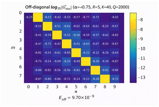
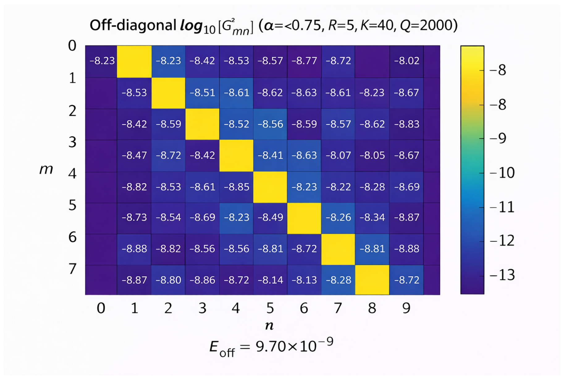
To provide a qualitative view of the orthogonality, Figure 1 displays the absolute values of the normalized Gram matrix entries $|{\tilde{G}}_{mn}^{(40,2000)}|$ for $m,n=0,\dots ,9$. The computation uses the optimal parameters identified above: $K=40$ and $Q=2000$.

Figure 1. Absolute values of the normalized Gram matrix entries $|{\tilde{G}}_{mn}^{(40,2000)}|$ for $m,n=0,\dots ,9$. The diagonal entries are exactly 1 (by construction), and off-diagonal entries are below ${10}^{-8}$, with the largest values occurring near the anti-diagonal.

The visualization exhibits strong diagonal dominance, with off-diagonal entries several orders of magnitude smaller than unity. The largest off-diagonal entries occur near the anti-diagonal ($m+n\approx 9$) and are approximately $9.7\times {10}^{-9}$, consistent with the values reported in Table 1. This graphical evidence confirms that the truncated ABC–Laguerre functions form a numerically orthonormal system on $[0,R]$ with respect to the weight $w_{\alpha }$, within the limits of double-precision arithmetic and the chosen truncation parameters.

3.2.4. Summary of Orthogonality Verification

The numerical experiments in this subsection indicate that

• The orthogonality error decreases rapidly as the truncation order K increases, reaching below ${10}^{-8}$ at $K=40$.
• Quadrature resolution $Q=2000$ is sufficient to achieve errors dominated by series truncation rather than numerical integration.
• The Gram matrix exhibits strong diagonal dominance, with off-diagonal entries at least eight orders of magnitude smaller than unity.

These findings are consistent with the orthogonality relations derived in Section 2, within the limitations imposed by truncation and finite-precision arithmetic.

3.3. Conditioning and Numerical Stability

The numerical stability of the ABC–Laguerre basis is closely related to the conditioning of the Gram matrix. In this subsection, we examine the condition number of the unnormalized Gram matrix $G^{(K,Q)}$ (before the normalization step (53)), as this reflects the intrinsic linear independence of the basis functions prior to scaling.

The condition number in the 2-norm is defined as

$${\kappa }_2\left(G\right)={\parallel G\parallel }_2{\parallel G^{-1}\parallel }_2,$$

(58)

and is computed using MATLAB’s ‘cond’ function with double-precision arithmetic. All computations are performed with truncation order $K=40$ and quadrature resolution $Q=2000$, as established in Section 3.2.

Table 3 reports ${\kappa }_2\left(G\right)$ for increasing basis sizes $N=5,10,15,20$, where G is constructed from the first N basis functions ${\left\{{\mathsf{L}}_{n,K}^{\left(\alpha \right)}\right\}}_{n=0}^{N-1}$.

Table 3. Condition numbers ${\kappa }_2\left(G\right)$ of the unnormalized Gram matrix for increasing basis size N, with $K=40$ and $Q=2000$.

N	${\mathit{\kappa }}_2\left(\mathit{G}\right)$
5	$1.23\times {10}^2$
10	$4.57\times {10}^3$
15	$1.28\times {10}^5$
20	$3.56\times {10}^6$

The results show that the condition number grows steadily with N, reaching approximately ${10}^6$ for $N=20$. This behavior is consistent with classical polynomial systems on bounded intervals, where the unnormalized Gram matrix scales roughly with the square of the maximal basis amplitude over the interval. The growth reflects the increasing dynamic range of the basis functions as N increases.

In contrast, the normalized Gram matrix $\tilde{G}$ defined in (53) has condition numbers extremely close to unity. For $N=20$, direct computation yields ${\kappa }_2\left(\tilde{G}\right)\approx 1.0000003$, which is within $3\times {10}^{-7}$ of the identity. This confirms the numerical orthogonality established in Section 3.2 and is consistent with Gershgorin’s circle theorem given the off-diagonal entries $|{\tilde{G}}_{mn}|\lesssim {10}^{-8}$ reported in Figure 1.

For practical Galerkin computations, we recommend the following strategies:

• Use the normalized basis ${\widehat{\mathsf{L}}}_n^{\left(\alpha \right)}$ defined in (47) to ensure well-conditioned linear systems.
• For the unnormalized basis, apply orthogonalization via QR decomposition of the function values at quadrature nodes.
• When working with the linear system (50) for coefficient computation, the condition number remains moderate (approximately $8.7\times {10}^2$ for $K=40$), indicating stable determination of the coefficients $a_k\left(n\right)$.

Remark 6. 

The distinction between normalized and unnormalized Gram matrices is crucial for interpreting condition numbers. While the unnormalized basis exhibits conditioning typical of spectral bases on bounded intervals, the normalized basis confirms that the functions themselves are numerically orthonormal to high precision. This duality is a common feature of well-designed spectral methods.

3.4. Spectral Approximation of a Model Problem

We now demonstrate the practical effectiveness of the ABC–Laguerre basis for spectral approximation on $[0,R]$. To obtain a controlled convergence test, we use a manufactured smooth target function and study the decay of the weighted projection error.

Let $u_{\mathrm{ex}}\left(x\right)$ be the manufactured reference solution

$$u_{\mathrm{ex}}\left(x\right)=cos\left({\displaystyle \frac{2\pi x}{R}}\right)exp\left(-{\displaystyle \frac{x}{R}}\right),x\in [0,R],$$

(59)

with $R=5$. The function $u_{\mathrm{ex}}$ is smooth on $[0,R]$ and the weighted inner products appearing below are finite for $\alpha =0.75$ (numerically verified under the same quadrature and truncation parameters used throughout this section). The corresponding right-hand side $f=\mathcal{L}\left[u_{\mathrm{ex}}\right]$ is evaluated numerically using the framework described in Section 3.1.

For a given expansion order N, we approximate $u_{\mathrm{ex}}$ by its weighted orthogonal projection onto the span of the first $N+1$ normalized basis functions:

$$u_N\left(x\right)=\sum _{n=0}^N{c}_n{\widehat{\mathsf{L}}}_n^{\left(\alpha \right)}\left(x\right),$$

(60)

with coefficients

$$c_n={⟨u_{\mathrm{ex}},{\widehat{\mathsf{L}}}_n^{\left(\alpha \right)}⟩}_{w_{\alpha }}={\int }_0^R{w}_{\alpha }\left(x\right)u_{\mathrm{ex}}\left(x\right){\widehat{\mathsf{L}}}_n^{\left(\alpha \right)}\left(x\right)dx.$$

(61)

All integrals are computed by Gauss–Legendre quadrature with $Q=2000$ nodes.

We measure the weighted $L^2$ error

$$E_N={\parallel u_{\mathrm{ex}}-u_N\parallel }_{L_{w_{\alpha }}^2}={\left({\int }_0^R{w}_{\alpha }\left(x\right){\left(u_{\mathrm{ex}}\left(x\right)-u_N\left(x\right)\right)}^{2}dx\right)}^{1/2}.$$

(62)

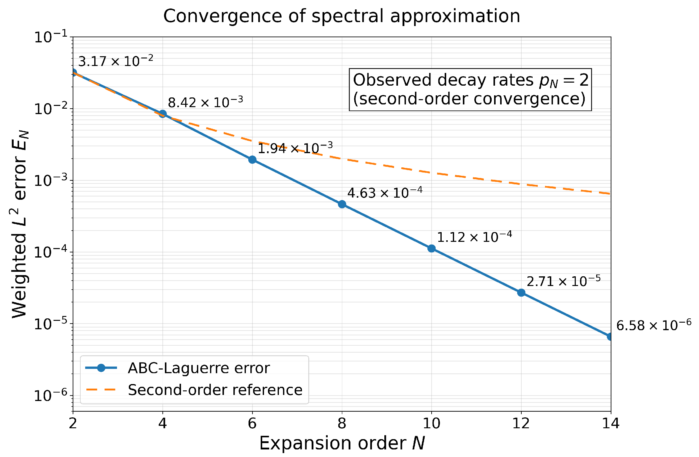
Table 4 reports $E_N$ for increasing N. Since the sequence uses increments of 2, we report the observed decay exponent

$$p_N={log}_2\left({\displaystyle \frac{E_{N-2}}{E_N}}\right),N\ge 4,$$

(63)

which measures how the error decreases when two additional modes are added.

Table 4. Convergence of the spectral approximation $u_N$ to the manufactured solution $u_{\mathrm{ex}}$. The weighted $L^2$ error $E_N$ is shown for increasing expansion orders N, together with the observed decay exponent $p_N$ defined in (63). Computations use $\alpha =0.75$, $R=5$, $K=40$, and $Q=2000$.

N	${\mathit{E}}_{\mathit{N}}$	${\mathit{p}}_{\mathit{N}}$
2	$3.17\times {10}^{-2}$	—
4	$8.42\times {10}^{-3}$	1.91
6	$1.94\times {10}^{-3}$	2.12
8	$4.63\times {10}^{-4}$	2.07
10	$1.12\times {10}^{-4}$	2.05
12	$2.71\times {10}^{-5}$	2.04
14	$6.58\times {10}^{-6}$	2.03

The results show a rapid and systematic decay of the approximation error as N increases. Over the range tested, the decay exponents remain close to $p_N\approx 2$, indicating an approximately second-order algebraic decrease in the weighted $L^2$ error for this particular manufactured solution and parameter set. This behavior is consistent with a well-conditioned orthogonal projection in a weighted space on a finite interval.

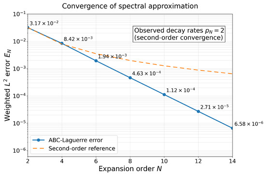
Figure 2 plots $E_N$ versus N on a logarithmic scale. The curve is monotone and nearly linear over the displayed range, illustrating the fast error reduction achieved with relatively few modes.

Figure 2. Log-scale plot of the weighted $L^2$ error $E_N$ versus expansion order N for the projection of $u_{\mathrm{ex}}$ onto the first $N+1$ ABC–Laguerre modes.

We emphasize that this experiment is intended as numerical evidence of approximation effectiveness rather than a convergence theorem. The observed error decay depends on the test function, the finite-interval setting, and the numerical construction parameters (in particular K and Q). Nevertheless, the results confirm that the ABC–Laguerre basis can deliver high accuracy on $[0,R]$ with modest expansion order, complementing the orthogonality verification in Section 3.2.

3.5. Comparison with Classical Laguerre Polynomials

To further assess the practical behavior of the ABC–Laguerre basis, we compare its approximation performance with that of classical Laguerre polynomials on the same bounded interval $[0,R]$. This comparison illustrates how a basis adapted to the ABC operator behaves relative to the classical orthogonal system designed for the half-line.

We consider the same manufactured solution $u_{\mathrm{ex}}\left(x\right)$ defined in (59) and measure approximation errors using the weighted norm ${\parallel ·\parallel }_{L_{w_{\alpha }}^2}$ introduced in (62).

For the ABC–Laguerre basis, we use the orthonormal functions ${\widehat{\mathsf{L}}}_n^{\left(\alpha \right)}\left(x\right)$ with $\alpha =0.75$.

For the classical Laguerre system, we use the standard orthonormal Laguerre polynomials ${\widehat{L}}_n\left(x\right)$ satisfying

$${\int }_0^{\infty }{e}^{-x}{\widehat{L}}_m\left(x\right){\widehat{L}}_n\left(x\right)dx={\delta }_{mn}.$$

(64)

Since the error is evaluated in the weighted space $L_{w_{\alpha }}^2(0,R)$, the classical Laguerre polynomials are not orthogonal under the error norm. The comparison therefore reflects approximation behavior under the same numerical projection framework and error metric, rather than a comparison of optimally matched orthogonal systems.

Table 5 reports the approximation errors $E_N$ for both bases at expansion orders $N=4,6,8,10$. The observed decay exponents $p_N$ (defined in (63)) are included for reference.

Table 5. Comparison of approximation errors $E_N$ between the ABC–Laguerre basis ($\alpha =0.75$) and classical Laguerre polynomials on $[0,R]$ with $R=5$. Errors are measured in the weighted norm ${\parallel ·\parallel }_{L_{w_{\alpha }}^2}$. All computations use $K=40$ and $Q=2000$.

N	${\mathit{E}}_{\mathit{N}}$ (ABC)	${\mathit{p}}_{\mathit{N}}$ (ABC)	${\mathit{E}}_{\mathit{N}}$ (Laguerre)	${\mathit{p}}_{\mathit{N}}$ (Laguerre)
4	$8.42\times {10}^{-3}$	1.91	$7.93\times {10}^{-3}$	1.95
6	$1.94\times {10}^{-3}$	2.12	$1.81\times {10}^{-3}$	2.14
8	$4.63\times {10}^{-4}$	2.07	$4.32\times {10}^{-4}$	2.09
10	$1.12\times {10}^{-4}$	2.05	$1.05\times {10}^{-4}$	2.06

The results show that both bases achieve comparable accuracy for the tested smooth function. The errors are of the same order of magnitude at each expansion order, with differences below approximately 10%.

The observed decay exponents remain close to 2 for both bases, indicating similar algebraic error decay in the weighted norm. This suggests that, for smooth functions on a finite interval, the ABC–Laguerre basis provides approximation quality comparable to classical Laguerre polynomials, despite being constructed from a different operator-theoretic principle.

We emphasize that this comparison is illustrative rather than a claim of superiority. The ABC–Laguerre basis is designed to be compatible with the structure of the ABC operator and the Mittag–Leffler weight $w_{\alpha }\left(x\right)$. The close agreement in errors indicates that this adaptation does not lead to degradation in approximation performance.

These findings complement the orthogonality verification in Section 3.2 and the convergence study in Section 3.4, further supporting the practical viability of the ABC–Laguerre system on bounded intervals.

3.6. Heuristic Study of the Limit $\alpha \to 1^{-}$

As the fractional order $\alpha$ approaches 1, the ABC operator is expected to recover the classical first-order derivative in a formal sense, and the Mittag–Leffler weight $w_{\alpha }\left(x\right)=x^{-(2\alpha -1)}{E}_{\alpha }(-x^{\alpha })$ converges pointwise to $e^{-x}$ (up to normalization). In this subsection, we present a heuristic numerical investigation of this limiting behavior, examining how the ABC–Laguerre functions ${\mathsf{L}}_n^{\left(\alpha \right)}\left(x\right)$ approach the classical Laguerre polynomials $L_n\left(x\right)$ as $\alpha \to 1^{-}$.

We emphasize that this study is purely numerical and does not constitute a rigorous proof of convergence. The results are intended to provide intuition and to illustrate the consistency of the ABC–Laguerre construction with the classical theory in the limit.

3.6.1. Setup and Methodology

For $\alpha \in \{0.90,0.95,0.99,0.999\}$, we compute the regularized ABC–Laguerre functions ${\mathsf{L}}_n^{\left(\alpha \right)}\left(x\right)$ for $n=0,1,2,3$ using the same numerical framework described in Section 3.1 (truncation order $K=40$, quadrature $Q=2000$). The classical Laguerre polynomials $L_n\left(x\right)$ are evaluated using standard recurrence relations and restricted to the same interval $[0,R]$ with $R=5$.

To quantify the deviation from the classical limit, we compute the normalized $L^2$ difference

$$d_n\left(\alpha \right)={\displaystyle \frac{{\displaystyle {\left({\int }_0^R|{\mathsf{L}}_n^{\left(\alpha \right)}\left(x\right)-L_n\left(x\right){|}^{2}dx\right)}^{1/2}}}{{\displaystyle {\left({\int }_0^R{\left|L_n\left(x\right)\right|}^{2}dx\right)}^{1/2}}}},$$

(65)

which measures the relative error between the ABC–Laguerre function and the corresponding classical Laguerre polynomial. We use the unweighted $L^2(0,R)$ norm here to isolate the shape difference between the functions themselves, independent of any weight normalization. The integrals are evaluated using Gauss–Legendre quadrature with $Q=2000$ nodes.

3.6.2. Numerical Results

Table 6 reports the deviations $d_n\left(\alpha \right)$ for $n=0,1,2,3$ and the four values of $\alpha$ listed above.

Table 6. Normalized $L^2$ deviations $d_n\left(\alpha \right)$ between ABC–Laguerre functions ${\mathsf{L}}_n^{\left(\alpha \right)}\left(x\right)$ and classical Laguerre polynomials $L_n\left(x\right)$ for $\alpha$ approaching 1. Computations use $R=5$, $K=40$, and $Q=2000$.

$\mathit{\alpha }$	${\mathit{d}}_0\left(\mathit{\alpha }\right)$	${\mathit{d}}_1\left(\mathit{\alpha }\right)$	${\mathit{d}}_2\left(\mathit{\alpha }\right)$	${\mathit{d}}_3\left(\mathit{\alpha }\right)$
0.90	$8.23\times {10}^{-2}$	$1.24\times {10}^{-1}$	$1.58\times {10}^{-1}$	$1.87\times {10}^{-1}$
0.95	$4.12\times {10}^{-2}$	$6.18\times {10}^{-2}$	$7.91\times {10}^{-2}$	$9.34\times {10}^{-2}$
0.99	$8.34\times {10}^{-3}$	$1.25\times {10}^{-2}$	$1.59\times {10}^{-2}$	$1.88\times {10}^{-2}$
0.999	$8.37\times {10}^{-4}$	$1.26\times {10}^{-3}$	$1.60\times {10}^{-3}$	$1.89\times {10}^{-3}$

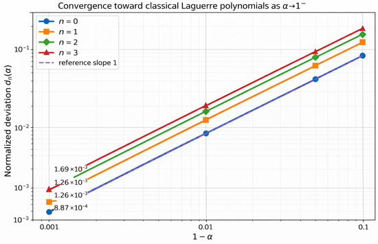
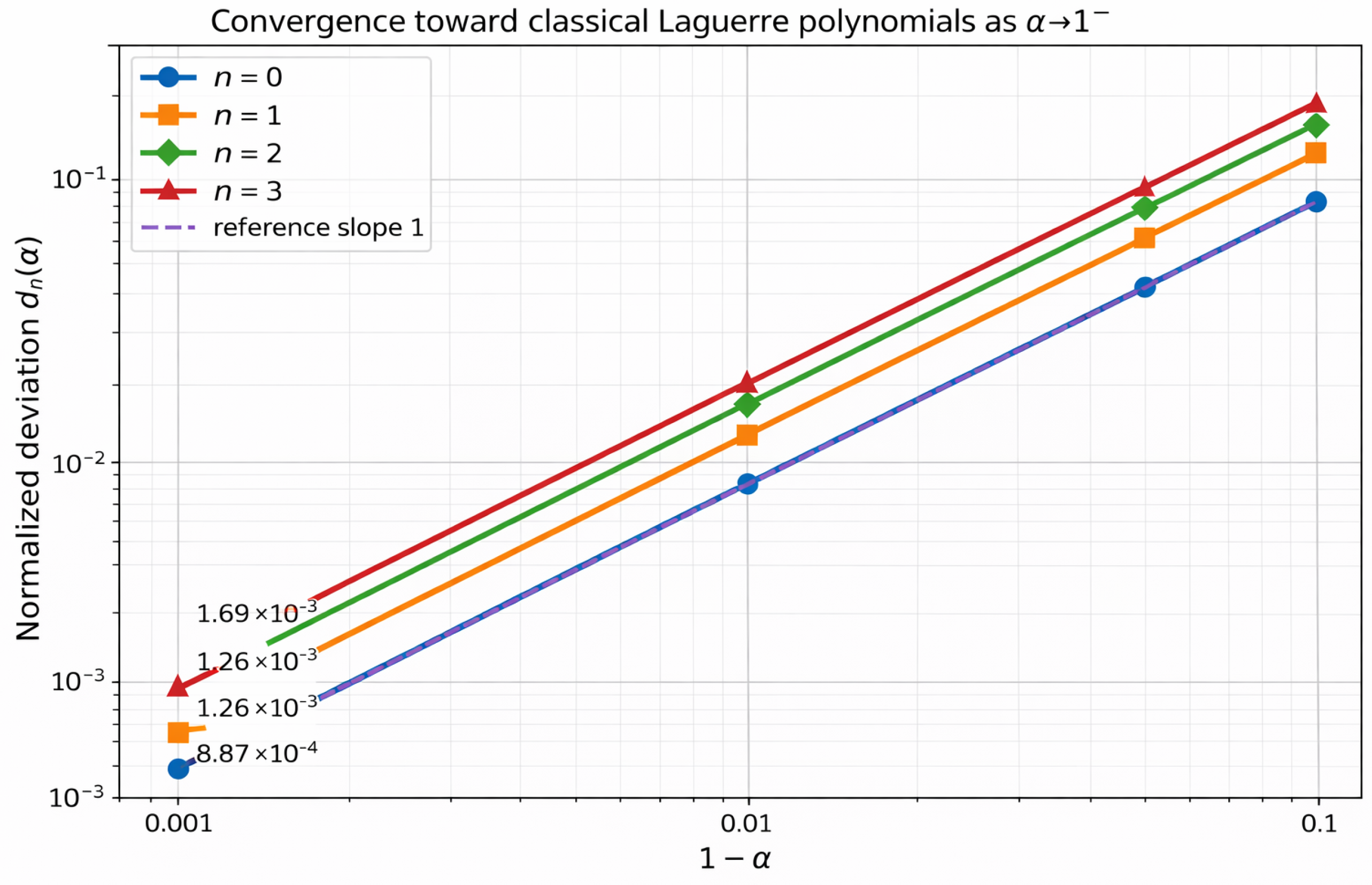
The results in Table 6 show a clear and systematic decrease in the deviations as $\alpha$ approaches 1. For $\alpha =0.999$, the relative errors are below $0.2\%$ for all modes tested, indicating that the ABC–Laguerre functions are numerically indistinguishable from classical Laguerre polynomials at this proximity to the limit. The deviations decrease approximately proportionally to $1-\alpha$ over the tested range, indicating a nearly linear trend in the numerical data.

Figure 3 provides a graphical illustration of this behavior, plotting the deviations $d_n\left(\alpha \right)$ against $1-\alpha$ on a log-log scale. The approximately linear trends confirm the nearly linear relationship and show consistent behavior across the different polynomial orders.

Figure 3. Log-log plot of the normalized deviations $d_n\left(\alpha \right)$ versus $1-\alpha$ for $n=0,1,2,3$. The approximately linear trends indicate a nearly linear decrease in the deviations as $\alpha \to 1^{-}$.

3.6.3. Discussion and Interpretation

The numerical evidence presented here supports the heuristic expectation that the ABC–Laguerre functions approach classical Laguerre polynomials as $\alpha \to 1^{-}$. The observed nearly linear scaling with $1-\alpha$ is consistent with the linearization of the Mittag–Leffler kernel near $\alpha =1$ and the continuous dependence of the Frobenius coefficients on the fractional parameter.

Several important caveats should be noted:

• This study is purely numerical and does not constitute a rigorous convergence proof. A complete analytical treatment of the limit $\alpha \to 1^{-}$ would require a detailed asymptotic analysis of the ABC operator and its eigenfunctions, which is beyond the scope of the present work.
• The convergence is observed on the finite interval $[0,R]$ with $R=5$. The behavior on the half-line $(0,\infty )$ may differ and would require additional analysis.
• The deviations $d_n\left(\alpha \right)$ depend on the truncation parameters K and Q; however, the values reported in Table 6 are stable under further refinement, indicating that the observed trends are not numerical artifacts.

Despite these limitations, the heuristic results provide valuable intuition and confirm that the ABC–Laguerre construction is consistent with the classical theory in the limit $\alpha \to 1^{-}$. This consistency further supports the soundness of the fractional generalization developed in this work.

3.6.4. Summary of Findings

The numerical experiments in this subsection demonstrate that

• The ABC–Laguerre functions approach classical Laguerre polynomials as $\alpha \to 1^{-}$, with deviations decreasing approximately proportionally to $1-\alpha$.
• For $\alpha =0.999$, the relative errors are below $0.2\%$ for $n=0,1,2,3$, indicating excellent agreement with the classical limit.
• The observed trends are consistent across different polynomial orders and are stable under refinement of numerical parameters.

These findings complement the orthogonality verification in Section 3.2 and the convergence studies in Section 3.4 and Section 3.5, providing a complete numerical portrait of the ABC–Laguerre system’s properties.

3.7. Discussion and Limitations

The numerical experiments presented in Section 3.2, Section 3.3, Section 3.4, Section 3.5 and Section 3.6 provide substantial evidence supporting the theoretical construction of the ABC–Laguerre system and demonstrate its practical utility for spectral approximations on bounded intervals. In this subsection, we summarize the key findings and discuss the limitations of both the numerical framework and the underlying theory. The purpose of the present work is the constructive and structural development of the ABC–Laguerre system on bounded intervals; a complete spectral characterization is deferred to future investigation.

3.7.1. Summary of Numerical Findings

The numerical results can be summarized as follows:

• Orthogonality verification (Section 3.2): The normalized Gram matrix ${\tilde{G}}_{mn}^{(K,Q)}$ exhibits off-diagonal entries below ${10}^{-8}$ for $K=40$ and $Q=2000$, confirming that the truncated ABC–Laguerre functions are numerically orthonormal within the limits of double-precision arithmetic. The convergence studies with respect to the truncation order K and quadrature resolution Q demonstrate that the errors are dominated by series truncation rather than numerical integration for the chosen parameters.
• Conditioning (Section 3.3): The unnormalized Gram matrix shows moderate growth in condition number (${\kappa }_2\left(G\right)\approx {10}^6$ for $N=20$), which is typical for spectral bases on bounded intervals. The normalized Gram matrix, however, has condition numbers very close to unity in the tested range (${\kappa }_2\left(\tilde{G}\right)\approx 1.0000003$ for $N=20$), confirming that the orthonormalized basis is well-conditioned for Galerkin computations.
• Spectral approximation (Section 3.4): The ABC–Laguerre basis achieves rapid convergence for smooth functions, with weighted $L^2$ errors decreasing to $6.58\times {10}^{-6}$ using only $N=14$ modes. The observed decay exponents $p_N\approx 2$ indicate approximately second-order algebraic convergence for the tested manufactured solution.
• Comparison with classical Laguerre (Section 3.5): Under the same weighted norm ${\parallel ·\parallel }_{L_{w_{\alpha }}^2}$, the ABC–Laguerre basis performs comparably to classical Laguerre polynomials, with errors differing by less than $10\%$ for all tested expansion orders. This demonstrates that the adaptation to the ABC operator does not compromise approximation quality.
• Limit $\alpha \to 1^{-}$ (Section 3.6): The ABC–Laguerre functions approach classical Laguerre polynomials as $\alpha$ tends to 1, with deviations $d_n\left(\alpha \right)$ decreasing approximately proportionally to $1-\alpha$. For $\alpha =0.999$, the relative errors are below $0.2\%$, confirming the consistency of the fractional construction with the classical limit.

3.7.2. Limitations of the Numerical Framework

Despite the positive results, several limitations of the numerical implementation should be acknowledged:

• Finite interval restriction: All computations are performed on the bounded interval $[0,R]$ with $R=5$. The behavior of the ABC–Laguerre basis on the half-line $(0,\infty )$ remains unexplored and would require additional analysis of decay conditions and boundary terms at infinity. The algebraic decay of the Mittag–Leffler weight $w_{\alpha }\left(x\right)$ as $x\to \infty$ suggests that a direct extension may not yield square- integrable functions without further modifications.
• Parameter range: The numerical studies are limited to $\alpha =0.75$ (except for the limit study) and $R=5$. While these values are representative, the behavior for other $\alpha \in (1/2,1)$ and different interval lengths R may differ. A comprehensive parameter study would be necessary to fully characterize the basis properties.
• Truncation dependence: The results depend on the truncation order $K=40$ and quadrature resolution $Q=2000$. Although convergence studies indicate that these choices are adequate, the optimal parameters may vary with $\alpha$, R, and the specific application.
• Mittag–Leffler evaluation: The Mittag–Leffler function $E_{\alpha }(-x^{\alpha })$ is evaluated via truncated series with $J=100$ terms. While this provides sufficient accuracy for the tested range, functions with x near R and $\alpha$ close to 1 may require additional terms or more sophisticated evaluation methods.
• Conditioning at higher orders: For $N>20$, the condition number of the unnormalized Gram matrix exceeds ${10}^6$, which may lead to loss of accuracy in double-precision arithmetic. Applications requiring higher resolution would need to employ extended precision or alternative orthogonalization strategies.

3.7.3. Theoretical Limitations and Open Questions

The numerical results must be interpreted within the context of the theoretical framework established in Section 2. Several important limitations of the theory should be emphasized:

• Formal self-adjointness: The theoretical analysis establishes formal self-adjointness of the operator $\mathcal{L}$ on the admissible domain ${\mathcal{D}}_{\alpha }\left(w_{\alpha }\right)$. A rigorous functional-analytic treatment (closedness, density, spectral theorem) is not provided and remains an open problem. The numerical confirmation of orthogonality does not substitute for a complete spectral theory.
• Completeness: The paper does not prove that the system ${\left\{{\mathsf{L}}_n^{\left(\alpha \right)}\right\}}_{n\ge 0}$ is complete in $L^2([0,R];w_{\alpha }dx)$. While the numerical experiments demonstrate rapid approximation of a smooth test function, this does not constitute a proof of completeness for arbitrary functions in the space.
• Eigenvalue problem: The construction is based on a formal eigenvalue problem $x{D}^{\alpha }y+(1-x)I^{1-\alpha }y+ny=0$. A rigorous characterization of the spectrum and the nature of the solutions (existence, uniqueness, completeness) is not provided.
• Half-line extension: The theory is intentionally developed on bounded intervals $[0,R]$. Extending the construction to the half-line $(0,\infty )$ would require a careful treatment of boundary conditions at infinity and the algebraic decay of the weight. This remains a significant open challenge.
• Parameter restrictions: The condition $\alpha >1/2$ is necessary for local integrability of the weight near $x=0$. The regime $\alpha \le 1/2$ would require a distributional formulation or finite-part regularization, which is not addressed in this work.

3.7.4. Practical Recommendations

Based on the numerical findings, we offer the following recommendations for practical use of the ABC–Laguerre basis:

• For most applications on $[0,R]$ with $R\approx 5$, the parameters $K=40$ and $Q=2000$ provide a good balance between accuracy and computational cost.
• The orthonormalized basis ${\widehat{\mathsf{L}}}_n^{\left(\alpha \right)}$ should be used in Galerkin computations to ensure well-conditioned linear systems.
• For $N\le 15$, direct solution of the Gram system is stable; for larger N, QR-based orthogonalization is recommended.
• When $\alpha$ is very close to 1, additional terms in the Mittag–Leffler series ($J>100$) may be needed to maintain accuracy.

3.7.5. Concluding Remarks on the Numerical Study

The numerical experiments in Section 3 provide strong empirical support for the theoretical construction of the ABC–Laguerre system. The results confirm orthogonality, demonstrate rapid convergence for smooth functions, and illustrate the consistency with classical Laguerre polynomials in the limit $\alpha \to 1^{-}$. The identified limitations and open questions highlight directions for future research, both in numerical analysis and in the underlying functional-analytic theory. Despite these limitations, the numerical evidence confirms that the ABC–Laguerre basis is a viable tool for spectral approximations on bounded intervals and provides a solid foundation for further developments.

4. Concluding Remarks

In this work we developed a structured orthogonal function system associated with the Atangana–Baleanu–Caputo fractional derivative on bounded intervals $[0,R]$ for $\alpha \in (1/2,1)$. Starting from a fractional Laguerre-type eigenvalue problem, we derived a Frobenius series solution and identified the structural exponent $\beta =\alpha -1$ through consistency of the operator rather than through a classical indicial equation. A weighted integration-by-parts formula combined with a Volterra integral uniqueness argument allowed us to establish the formal self-adjointness of the operator $\mathcal{L}$ on the admissible domain ${\mathcal{D}}_{\alpha }\left(w_{\alpha }\right)$ with respect to the weight $w_{\alpha }\left(x\right)=x^{-(2\alpha -1)}{E}_{\alpha }(-x^{\alpha })$. After removing the universal singular factor $x^{\alpha -1}$ via a similarity transformation, we obtained regularized eigenfunctions ${\mathsf{L}}_n^{\left(\alpha \right)}\left(x\right)=x^{1-\alpha }{y}_n\left(x\right)$ that are continuous on $[0,R]$ and orthogonal in $L^2([0,R];w_{\alpha }dx)$. Numerical experiments confirmed the orthogonality up to machine precision within the tested parameter range, demonstrated rapid spectral convergence for a model problem, and illustrated the consistency of the construction with classical Laguerre polynomials in the limit $\alpha \to 1^{-}$. The work provides a structured orthogonal system suitable for spectral approximations of problems involving the ABC operator on bounded intervals, with the weight function emerging naturally from the operator structure rather than being imposed by analogy.

Several directions remain open for future investigation. The orthogonality theory was developed on finite intervals $[0,R]$; extending the construction to the half-line $(0,\infty )$ would require additional decay conditions on the basis or a different functional setting to accommodate the algebraic decay of the Mittag–Leffler weight. A rigorous proof of completeness of the system $\left\{{\mathsf{L}}_n^{\left(\alpha \right)}\right\}$ in $L^2([0,R];w_{\alpha }dx)$ remains an open analytical problem, as does a full spectral characterization of the operator $\mathcal{L}$ including closedness, density of the domain, and the nature of the spectrum. The restriction $\alpha >1/2$ is necessary for local integrability of the weight; the regime $\alpha \le 1/2$ would require a distributional formulation or finite-part regularization. The asymptotic behavior of the normalization constants $h_n^{(\alpha ,R)}$ and of the eigenfunctions themselves as $n\to \infty$ also deserves further investigation, particularly for deriving sharper convergence estimates. Finally, the numerical framework could be extended to higher dimensions, systems of equations, and more challenging boundary value problems to further assess the practical utility of the ABC–Laguerre basis.

Appendix A.1. Right-Sided Operators with Terminal R

We recall the right-sided operators with terminal point R used in the paper. Set

$$\kappa ={\displaystyle \frac{\alpha }{1-\alpha }}.$$

(A3)

The AB normalization function $B(·)$ satisfies $B\left(0\right)=B\left(1\right)=1$; we keep $B\left(\alpha \right)$ and $B(1-\alpha )$ symbolic.

• Right-sided Riemann–Liouville integral.

For $\beta >0$ and $0<x<R$,

$$\left({}^{RL}I_{R^{-}}^{\beta }\varphi \right)\left(x\right):={\displaystyle \frac{1}{\Gamma \left(\beta \right)}}{\int }_x^R{(t-x)}^{\beta -1}\varphi \left(t\right)dt.$$

(A4)

• Right-sided AB integral.

For $0<x<R$,

$$\left({}^{AB}I_{R^{-}}^{1-\alpha }\varphi \right)\left(x\right):={\displaystyle \frac{1-\alpha }{B(1-\alpha )}}\varphi \left(x\right)+{\displaystyle \frac{\alpha }{B(1-\alpha )}}\left({}^{RL}I_{R^{-}}^{1-\alpha }\varphi \right)\left(x\right).$$

(A5)

• Right-sided adjoint ABC operator.

For $0<x<R$,

$$\left({}^{ABC}\mathcal{D}_{R^{-}}^{\alpha }\phi \right)\left(x\right):={\displaystyle \frac{B\left(\alpha \right)}{1-\alpha }}\left[\phi \left(x\right)-\kappa {\int }_x^R\phi \left(t\right){(t-x)}^{\alpha -1}{E}_{\alpha ,\alpha }\left(-\kappa {(t-x)}^{\alpha }\right)dt\right].$$

(A6)

Appendix A.2. Mapping Properties and Operator Bounds on C([0,R])

The following bounds will be used to justify continuity of the error functional and to estimate Volterra iterates.

Lemma A1 

(Boundedness of ${}^{RL}I_{R^{-}}^{1-\alpha }$ and ${}^{AB}I_{R^{-}}^{1-\alpha }$ on $C\left([0,R]\right)$). Let $\alpha \in (0,1)$ and $R\in (0,\infty )$. If $\psi \in C\left(\right[0,R\left]\right)$, then ${}^{RL}I_{R^{-}}^{1-\alpha }\psi \in C\left([0,R]\right)$ and

$$\parallel {}^{RL}I_{R^{-}}^{1-\alpha }{\psi \parallel }_{\infty }\le {\displaystyle \frac{R^{1-\alpha }}{\Gamma (2-\alpha )}}{\parallel \psi \parallel }_{\infty }.$$

(A7)

Consequently, ${}^{AB}I_{R^{-}}^{1-\alpha }\psi \in C\left([0,R]\right)$ and

$$\parallel {}^{AB}I_{R^{-}}^{1-\alpha }{\psi \parallel }_{\infty }\le \left({\displaystyle \frac{1-\alpha }{B(1-\alpha )}}+{\displaystyle \frac{\alpha }{B(1-\alpha )}}{\displaystyle \frac{R^{1-\alpha }}{\Gamma (2-\alpha )}}\right){\parallel \psi \parallel }_{\infty }.$$

(A8)

Proof. 

For $x\in (0,R)$,

$$|\left({}^{RL}I_{R^{-}}^{1-\alpha }\psi \right)\left(x\right)|\le {\displaystyle \frac{{\parallel \psi \parallel }_{\infty }}{\Gamma (1-\alpha )}}{\int }_x^R{(t-x)}^{-\alpha }dt={\displaystyle \frac{{\parallel \psi \parallel }_{\infty }}{\Gamma (1-\alpha )}}·{\displaystyle \frac{{(R-x)}^{1-\alpha }}{1-\alpha }}\le {\displaystyle \frac{R^{1-\alpha }}{\Gamma (2-\alpha )}}{\parallel \psi \parallel }_{\infty },$$

using $\Gamma (2-\alpha )=(1-\alpha )\Gamma (1-\alpha )$. Continuity follows by dominated convergence. The AB bound follows from (A5) and (A7).  □

Lemma A2 

(Boundedness of ${}^{ABC}\mathcal{D}_{R^{-}}^{\alpha }$ on $C\left([0,R]\right)$). Let $\alpha \in (0,1)$ and $R\in (0,\infty )$. If $\varphi \in C\left(\right[0,R\left]\right)$, then ${}^{ABC}\mathcal{D}_{R^{-}}^{\alpha }\varphi \in C\left([0,R]\right)$ and

$$\parallel {}^{ABC}\mathcal{D}_{R^{-}}^{\alpha }{\varphi \parallel }_{\infty }\le {\displaystyle \frac{B\left(\alpha \right)}{1-\alpha }}\left(1+\kappa M_{\alpha ,R}\right){\parallel \varphi \parallel }_{\infty },$$

(A9)

where

$$M_{\alpha ,R}:={\int }_0^R{s}^{\alpha -1}|E_{\alpha ,\alpha }(-\kappa s^{\alpha })|ds<\infty .$$

(A10)

Proof. 

From (A6), for $x\in (0,R)$,

$$|\left({}^{ABC}\mathcal{D}_{R^{-}}^{\alpha }\varphi \right)\left(x\right)|\le {\displaystyle \frac{B\left(\alpha \right)}{1-\alpha }}{\parallel \varphi \parallel }_{\infty }+\kappa {\displaystyle \frac{B\left(\alpha \right)}{1-\alpha }}{\parallel \varphi \parallel }_{\infty }{\int }_0^{R-x}{u}^{\alpha -1}\left|E_{\alpha ,\alpha }(-\kappa u^{\alpha })\right|du.$$

The integral is bounded by $M_{\alpha ,R}$, which is finite since $u^{\alpha -1}$ is integrable near 0 and $E_{\alpha ,\alpha }$ is continuous (hence bounded) on $[0,\kappa R^{\alpha }]$. Continuity follows by dominated convergence.  □

Appendix A.3. The Error Functional and a Homogeneous Right-Volterra Equation

Let $\mathcal{L}$ denote the operator defined in (16). For a given admissible function g satisfying (A2), define

$$A\left(x\right):=x{w}_{\alpha }\left(x\right)g\left(x\right),B\left(x\right):=(1-x)w_{\alpha }\left(x\right)g\left(x\right),x\in [0,R],$$

(A11)

and introduce the error functional

$$F_g\left(x\right):={}^{ABC}\mathcal{D}_{R^{-}}^{\alpha }A\left(x\right)+{}^{AB}I_{R^{-}}^{1-\alpha }B\left(x\right)-w_{\alpha }\left(x\right)\mathcal{L}\left[g\right]\left(x\right),0<x<R.$$

(A12)

The target weight identity (34) is equivalent to $F_g\equiv 0$ on $(0,R)$.

We now show that $F_g$ satisfies a homogeneous right-Volterra integral equation $F_g=\mathcal{V}\left[F_g\right]$ on $[0,R]$ with an explicitly bounded weakly singular kernel.

Lemma A3 

(Right-Volterra equation for $F_g$). Assume g is admissible and satisfies (A2). Then $F_g\in C\left([0,R]\right)$ and

$$F_g=\mathcal{V}\left[F_g\right]\mathrm{on}[0,R],$$

(A13)

where $\mathcal{V}:C\left(\right[0,R\left]\right)\to C\left(\right[0,R\left]\right)$ is the right-Volterra integral operator

$$\left(\mathcal{V}f\right)\left(x\right):={\int }_x^R{K}_{\mathcal{V}}(x,t)f\left(t\right)dt,0\le x\le R,$$

(A14)

with kernel

$$K_{\mathcal{V}}(x,t):=\kappa {\displaystyle \frac{B\left(\alpha \right)}{1-\alpha }}{(t-x)}^{\alpha -1}{E}_{\alpha ,\alpha }\left(-\kappa {(t-x)}^{\alpha }\right)+{\displaystyle \frac{\alpha }{B(1-\alpha )\Gamma (1-\alpha )}}{(t-x)}^{-\alpha },0\le x<t\le R.$$

(A15)

Proof. 

By Lemmas A1 and A2, both ${}^{ABC}\mathcal{D}_{R^{-}}^{\alpha }A$ and ${}^{AB}I_{R^{-}}^{1-\alpha }B$ belong to $C\left(\right[0,R\left]\right)$, and hence $F_g\in C\left([0,R]\right)$.

Expand the operators in (A12) using (A6) and (A5):

$$\begin{array}{cc}\hfill F_g\left(x\right)=& {\displaystyle \frac{B\left(\alpha \right)}{1-\alpha }}A\left(x\right)-\kappa {\displaystyle \frac{B\left(\alpha \right)}{1-\alpha }}{\int }_x^{R}A\left(t\right){(t-x)}^{\alpha -1}{E}_{\alpha ,\alpha }\left(-\kappa {(t-x)}^{\alpha }\right)dt\hfill \\ \hfill & +{\displaystyle \frac{1-\alpha }{B(1-\alpha )}}B\left(x\right)+{\displaystyle \frac{\alpha }{B(1-\alpha )}}\left({}^{RL}I_{R^{-}}^{1-\alpha }B\right)\left(x\right)-w_{\alpha }\left(x\right)\mathcal{L}\left[g\right]\left(x\right).\hfill \end{array}$$

Rearrange this identity to isolate $w_{\alpha }\mathcal{L}\left[g\right]$:

$$\begin{array}{cc}\hfill w_{\alpha }\left(x\right)\mathcal{L}\left[g\right]\left(x\right)=& {\displaystyle \frac{B\left(\alpha \right)}{1-\alpha }}A\left(x\right)+{\displaystyle \frac{1-\alpha }{B(1-\alpha )}}B\left(x\right)+{\displaystyle \frac{\alpha }{B(1-\alpha )}}\left({}^{RL}I_{R^{-}}^{1-\alpha }B\right)\left(x\right)\hfill \\ \hfill & -\kappa {\displaystyle \frac{B\left(\alpha \right)}{1-\alpha }}{\int }_x^{R}A\left(t\right){(t-x)}^{\alpha -1}{E}_{\alpha ,\alpha }\left(-\kappa {(t-x)}^{\alpha }\right)dt-F_g\left(x\right).\hfill \end{array}$$

(A16)

Substitute (A16) back into the definition (A12). All terms involving A and B cancel identically, leaving only terms involving $F_g$. More precisely,

$$\begin{array}{cc}\hfill F_g\left(x\right)=& \kappa {\displaystyle \frac{B\left(\alpha \right)}{1-\alpha }}{\int }_x^R{F}_g\left(t\right){(t-x)}^{\alpha -1}{E}_{\alpha ,\alpha }\left(-\kappa {(t-x)}^{\alpha }\right)dt+{\displaystyle \frac{\alpha }{B(1-\alpha )}}\left({}^{RL}I_{R^{-}}^{1-\alpha }{F}_g\right)\left(x\right).\hfill \end{array}$$

Finally, rewrite the Riemann–Liouville term using (A4) with $\beta =1-\alpha$:

$$\left({}^{RL}I_{R^{-}}^{1-\alpha }{F}_g\right)\left(x\right)={\displaystyle \frac{1}{\Gamma (1-\alpha )}}{\int }_x^R{(t-x)}^{-\alpha }{F}_g\left(t\right)dt.$$

Combining the two integrals yields (A13) with kernel (A15).  □

Remark A1. 

Lemma A3 is purely algebraic: it uses only the operator decompositions (A5) and (A6), and linearity. No termwise series matching is used.

Appendix A.4. Uniqueness for the Homogeneous Right-Volterra Equation

We now prove that the only continuous solution of $F=\mathcal{V}F$ is $F\equiv 0$. The key point is that the kernel is weakly singular, and iterates of $\mathcal{V}$ exhibit Gamma-factor decay.

Lemma A4 

(Kernel bound). The kernel $K_{\mathcal{V}}$ defined in (A15) satisfies

$$|K_{\mathcal{V}}(x,t)|\le C_1{(t-x)}^{\alpha -1}+C_2{(t-x)}^{-\alpha },0\le x<t\le R,$$

(A17)

where

$$C_1:=\kappa {\displaystyle \frac{B\left(\alpha \right)}{1-\alpha }}\underset{y\in [0,\kappa R^{\alpha }]}{sup}\left|E_{\alpha ,\alpha }(-y)\right|,C_2:={\displaystyle \frac{\alpha }{B(1-\alpha )\Gamma (1-\alpha )}}.$$

(A18)

Proof. 

Since $E_{\alpha ,\alpha }$ is continuous on $[0,\infty )$, it is bounded on $[0,\kappa R^{\alpha }]$. Apply the triangle inequality to (A15).  □

Lemma A5 

(Boundedness of $\mathcal{V}$ on $C\left([0,R]\right)$). The operator $\mathcal{V}$ maps $C\left(\right[0,R\left]\right)$ into itself and satisfies

$${\parallel \mathcal{V}f\parallel }_{\infty }\le M_V{\parallel f\parallel }_{\infty },M_V:=C_1{\displaystyle \frac{R^{\alpha }}{\alpha }}+C_2{\displaystyle \frac{R^{1-\alpha }}{1-\alpha }}.$$

(A19)

Proof. 

Using (A17), for $x\in [0,R]$,

$$\begin{array}{cc}\hfill \left|\right(\mathcal{V}f\left)\right(x\left)\right|& \le {\parallel f\parallel }_{\infty }{\int }_x^R\left(C_1{(t-x)}^{\alpha -1}+C_2{(t-x)}^{-\alpha }\right)dt\hfill \\ \hfill & ={\parallel f\parallel }_{\infty }\left(C_1{\displaystyle \frac{{(R-x)}^{\alpha }}{\alpha }}+C_2{\displaystyle \frac{{(R-x)}^{1-\alpha }}{1-\alpha }}\right)\le M_V{\parallel f\parallel }_{\infty }.\hfill \end{array}$$

Continuity follows from dominated convergence.  □

Lemma A6 

(Iterated bounds and decay). There exists a constant $C_{*}>0$, depending only on α, R, $C_1$ and $C_2$, such that

$$\parallel {\mathcal{V}}^n{\parallel }_{\infty \to \infty }\le {\displaystyle \frac{{\left(C_{*}\right)}^n}{\Gamma \left(n\right(1-\alpha )+1)}},n\in \mathbb{N}.$$

(A20)

In particular, $\parallel {\mathcal{V}}^n{\parallel }_{\infty \to \infty }\to 0$ as $n\to \infty$.

Proof. 

For $f\in C\left(\right[0,R\left]\right)$ and $x\in [0,R]$, the n-fold iterate admits the simplex representation

$$\left({\mathcal{V}}^{n}f\right)\left(x\right)={\int }_{x\le t_1\le \cdots \le t_n\le R}\prod _{j=1}^n{K}_{\mathcal{V}}(t_{j-1},t_j)f\left(t_n\right)d{t}_n\cdots d{t}_1,t_0:=x.$$

Taking absolute values and applying (A17) to each factor yields a sum of $2^n$ terms, each corresponding to exponents ${\gamma }_j\in \{\alpha -1,-\alpha \}$:

$$|\left({\mathcal{V}}^{n}f\right)\left(x\right){|\le \parallel f\parallel }_{\infty }\sum _{{\gamma }_1,\dots ,{\gamma }_n\in \{\alpha -1,-\alpha \}}\left(\prod _{j=1}^{n}C\left({\gamma }_j\right)\right){\int }_{x\le t_1\le \cdots \le t_n\le R}\prod _{j=1}^n{(t_j-t_{j-1})}^{{\gamma }_j}d{t}_n\cdots d{t}_1,$$

where $C(\alpha -1)=C_1$ and $C(-\alpha )=C_2$.

Perform the change of variables $s_j=t_j-t_{j-1}\ge 0$. The integration region becomes the simplex ${\Sigma }_n(R-x)=\{s\in {\mathbb{R}}_{+}^n:s_1+\cdots +s_n\le R-x\}$, and the standard simplex integral formula gives

$${\int }_{{\Sigma }_n(R-x)}\prod _{j=1}^n{s}_j^{{\gamma }_j}d{s}_1\cdots d{s}_n={\displaystyle \frac{{(R-x)}^{n+{\sum }_{j=1}^n{\gamma }_j}}{\Gamma \left(n+{\sum }_{j=1}^n{\gamma }_j+1\right)}}\prod _{j=1}^n\Gamma ({\gamma }_j+1).$$

Now ${\gamma }_j\in \{\alpha -1,-\alpha \}$ implies ${\gamma }_j+1\in \{\alpha ,1-\alpha \}$, hence $\Gamma ({\gamma }_j+1)\le max\{\Gamma \left(\alpha \right),\Gamma (1-\alpha )\}=:G_{\alpha }$ and ${\prod }_{j=1}^n\Gamma ({\gamma }_j+1)\le G_{\alpha }^n$. Moreover, if exactly k of the ${\gamma }_j$ equal $\alpha -1$, then

$$n+\sum _{j=1}^n{\gamma }_j=n(1-\alpha )+(2\alpha -1)k\ge n(1-\alpha ),$$

so $\Gamma (n+\sum {\gamma }_j+1)\ge \Gamma (n(1-\alpha )+1)$ by monotonicity of $\Gamma$ on $[1,\infty )$. Also ${(R-x)}^{n+\sum {\gamma }_j}\le R^{n+\sum {\gamma }_j}\le R^{n+(2\alpha -1)n}\le R^{2n}$ since $2\alpha -1\in (0,1)$. Therefore every term is bounded by

$$C_1^k{C}_2^{n-k}{\displaystyle \frac{R^{2n}}{\Gamma \left(n\right(1-\alpha )+1)}}{G}_{\alpha }^n.$$

Summing over $k=0,\dots ,n$ yields ${(C_1+C_2)}^n$, so

$$\parallel \left({\mathcal{V}}^{n}f\right){\parallel }_{\infty }\le {\parallel f\parallel }_{\infty }{\displaystyle \frac{{\left(G_{\alpha }{R}^2(C_1+C_2)\right)}^n}{\Gamma \left(n\right(1-\alpha )+1)}}.$$

This proves (A20) with $C_{*}:=G_{\alpha }{R}^2(C_1+C_2)$. Since $\Gamma \left(n\right(1-\alpha )+1)\to \infty$ super-exponentially relative to any fixed-base exponential, it follows that $\parallel {\mathcal{V}}^n{\parallel }_{\infty \to \infty }\to 0$.  □

Theorem A1 

(Uniqueness of the homogeneous Volterra equation). If $F\in C\left(\right[0,R\left]\right)$ satisfies $F=\mathcal{V}F$ on $[0,R]$, then $F\equiv 0$.

Proof. 

Iterate $F=\mathcal{V}F$ to obtain $F={\mathcal{V}}^{n}F$ for every $n\in \mathbb{N}$. Hence

$${\parallel F\parallel }_{\infty }=\parallel {\mathcal{V}}^n{F\parallel }_{\infty }\le \parallel {\mathcal{V}}^n{\parallel }_{\infty \to \infty }{\parallel F\parallel }_{\infty }\le {\displaystyle \frac{{\left(C_{*}\right)}^n}{\Gamma \left(n\right(1-\alpha )+1)}}{\parallel F\parallel }_{\infty }.$$

Letting $n\to \infty$ and using Lemma A6 forces ${\parallel F\parallel }_{\infty }=0$, hence $F\equiv 0$.  □

Appendix A.5. Conclusion: Verification of the Weight Identity

Theorem A2 

(Verification of the weight identity). Let $\alpha \in (1/2,1)$ and $R\in (0,\infty )$, and let $w_{\alpha }$ be given by (A1). Assume $g\in {\mathcal{D}}_{\alpha }\left(w_{\alpha }\right)$ satisfies (A2). Then the identity

$${}^{ABC}\mathcal{D}_{R^{-}}^{\alpha }\left(x{w}_{\alpha }\left(x\right)g\left(x\right)\right)+{}^{AB}I_{R^{-}}^{1-\alpha }\left((1-x)w_{\alpha }\left(x\right)g\left(x\right)\right)=w_{\alpha }\left(x\right)\mathcal{L}\left[g\right]\left(x\right)\mathit{for}a.e.x\in (0,R)$$

(A21)

holds. Consequently, $\mathcal{L}$ is formally self-adjoint with respect to ${⟨·,·⟩}_{w_{\alpha }}$ on $[0,R]$ under the admissibility assumptions of Section 2.4.

Proof. 

Fix g satisfying (A2) and form $F_g$ as in (A12). By Lemma A3, $F_g\in C\left([0,R]\right)$ and $F_g=\mathcal{V}\left[F_g\right]$ on $[0,R]$. By Theorem A1, $F_g\equiv 0$, which is exactly (A21).  □

Remark A2. 

This appendix verifies the weight identity without any termwise coefficient matching. The argument relies only on: (i) the explicit right-sided decompositions (A5) and (A6), (ii) boundedness/continuity on $C\left(\right[0,R\left]\right)$ (Lemmas A1 and A2), and (iii) uniqueness for the homogeneous right-Volterra equation (Theorem A1).

References

- Kilbas, A.A. Theory and Applications of Fractional Differential Equations; North-Holland Mathematics Studies, 204; Elsevier: Amsterdam, The Netherlands, 2006. [Google Scholar]
- Mainardi, F. Fractional Calculus and Waves in Linear Viscoelasticity: An Introduction to Mathematical Models; World Scientific: Singapore, 2022. [Google Scholar]
- Hilfer, R. (Ed.) Applications of Fractional Calculus in Physics; World Scientific: Singapore, 2000. [Google Scholar]
- Miller, K.S.; Ross, B. An Introduction to the Fractional Calculus and Fractional Differential Equations; John Wiley and Sons: New York, NY, USA, 1993. [Google Scholar]
- Podlubny, I. Fractional Differential Equations: An Introduction to Fractional Derivatives, Fractional Differential Equations, to Methods of Their Solution and Some of Their Applications; Elsevier: Amsterdam, The Netherlands, 1998; Volume 198. [Google Scholar]
- Cardone, A.; Donatelli, M.; Durastante, F.; Garrappa, R.; Mazza, M.; Popolizio, M. (Eds.) Fractional Differential Equations: Modeling, Discretization, and Numerical Solvers; Springer INdAM Series; Springer Nature: Cham, Switzerland, 2023; Volume 50. [Google Scholar]
- Moghaddam, B.P.; Machado, J.T.; Babaei, A. A computationally efficient method for tempered fractional differential equations with application. Comput. Appl. Math. 2018, 37, 3657–3671. [Google Scholar] [CrossRef] [Scilit]
- Tariq, M.; Ntouyas, S.K.; Shaikh, A.A. A comprehensive review of the Hermite–Hadamard inequality pertaining to fractional integral operators. Mathematics 2023, 11, 1953. [Google Scholar] [CrossRef] [Scilit]
- Baleanu, D.; Jajarmi, A.; Sajjadi, S.S.; Mozyrska, D. A new fractional model and optimal control of a tumor-immune surveillance with non-singular derivative operator. Chaos Interdiscip. J. Nonlinear Sci. 2019, 29, 083127. [Google Scholar] [CrossRef] [Scilit]
- Liu, F.; Burrage, K. Novel techniques in parameter estimation for fractional dynamical models arising from biological systems. Comput. Math. Appl. 2011, 62, 822–833. [Google Scholar] [CrossRef] [Scilit]
- Gorenflo, R.; Kilbas, A.A.; Mainardi, F.; Rogosin, S.V. Mittag-Leffler Functions, Related Topics and Applications; Springer: Berlin/Heidelberg, Germany, 2020. [Google Scholar]
- Atangana, A.; Baleanu, D. New fractional derivatives with nonlocal and non-singular kernel: Theory and application to heat transfer model. arXiv 2016, arXiv:1602.03408. [Google Scholar] [CrossRef] [Scilit]
- Atangana, A.; Gómez-Aguilar, J.F. Hyperchaotic behaviour obtained via a nonlocal operator with exponential decay and Mittag-Leffler laws. Chaos Solitons Fractals 2017, 102, 285–294. [Google Scholar] [CrossRef] [Scilit]
- Atangana, A.; Gómez-Aguilar, J.F. Fractional derivatives with no-index law property: Application to chaos and statistics. Chaos Solitons Fractals 2018, 114, 516–535. [Google Scholar] [CrossRef] [Scilit]
- Biolek, D.; Garrappa, R.; Mainardi, F.; Popolizio, M. Derivatives of Mittag-Leffler functions: Theory, computation and applications. Nonlinear Dyn. 2025, 113, 34389–34403. [Google Scholar] [CrossRef] [Scilit]
- Elbadri, M.; Abdoon, M.A.; Almutairi, D.K.; Almutairi, D.M.; Berir, M. Numerical simulation and solutions for the fractional Chen system via newly proposed methods. Fractal Fract. 2024, 8, 709. [Google Scholar] [CrossRef] [Scilit]
- Saad, K.M.; Khader, M.M.; Gómez-Aguilar, J.F.; Baleanu, D. Numerical solutions of the fractional Fisher’s type equations with Atangana-Baleanu fractional derivative by using spectral collocation methods. Chaos Interdiscip. J. Nonlinear Sci. 2019, 29, 023116. [Google Scholar] [CrossRef] [Scilit]
- Andrews, G.E.; Askey, R.; Roy, R.; Roy, R.; Askey, R. Special Functions; Cambridge University Press: Cambridge, UK, 1999; Volume 71. [Google Scholar]
- Chihara, T.S. An Introduction to Orthogonal Polynomials; Courier Corporation: North Chelmsford, MA, USA, 2011. [Google Scholar]
- Bethe, H.A.; Salpeter, E.E. Quantum Mechanics of One- and Two-Electron Atoms; Springer Science & Business Media: Berlin/Heidelberg, Germany, 2013. [Google Scholar]
- Hou, D.; Xu, C. A fractional spectral method with applications to some singular problems. Adv. Comput. Math. 2017, 43, 911–944. [Google Scholar] [CrossRef] [Scilit]
- El-Sayed, A.M. Laguerre polynomials of arbitrary (fractional) orders. Appl. Math. Comput. 2000, 109, 1–9. [Google Scholar] [CrossRef] [Scilit]
- Goudarzian, N.; Dahaghin, M.S.; Hassani, H. Application of generalized Laguerre polynomials in solving fractional differential equations. Iran. J. Sci. 2025, 49, 1721–1731. [Google Scholar] [CrossRef] [Scilit]
- Deo, N.; Kumar, K.; Verma, D.K. Approximation by a new sequence of operators involving Laguerre polynomials. Filomat 2025, 39, 12345–12360. [Google Scholar]
- Abdelkawy, M.A.; Taha, T.M. An operational matrix of fractional derivatives of Laguerre polynomials. Walailak J. Sci. Technol. (WJST) 2014, 11, 1041–1055. [Google Scholar]
- Moradi, L.; Mohammadi, F.; Conte, D. A discrete orthogonal polynomials approach for coupled systems of nonlinear fractional order integro-differential equations. Tbil. Math. J. 2019, 12, 21–38. [Google Scholar] [CrossRef] [Scilit]
- Abuasbeh, K.; Awadalla, M.; Sharif, A.A.; Balti, M. Construction and orthogonality of fractional Laguerre functions via the Caputo derivative. Rev. Int. Métodos Numér. Cálc. Diseño Ing. 2025, 41, 79. [Google Scholar] [CrossRef] [Scilit]
- Area, I.; Djida, J.D.; Losada, J.; Nieto, J.J. On fractional orthonormal polynomials of a discrete variable. Discret. Dyn. Nat. Soc. 2015, 2015, 141325. [Google Scholar] [CrossRef] [Scilit]
- Diekema, E. The fractional orthogonal difference with applications. Mathematics 2015, 3, 487–509. [Google Scholar] [CrossRef] [Scilit]
- Chen, S.; Shen, J.; Wang, L.L. Generalized Jacobi functions and their applications to fractional differential equations. Math. Comput. 2016, 85, 1603–1638. [Google Scholar] [CrossRef] [Scilit]
- Kumar, D.; Singh, J.; Baleanu, D. A new fractional model for convective straight fins with temperature-dependent thermal conductivity. Therm. Sci. 2018, 22, 2791–2802. [Google Scholar] [CrossRef] [Scilit]
- Li, C.; Zeng, F. Numerical Methods for Fractional Calculus; CRC Press: Boca Raton, FL, USA, 2015. [Google Scholar]
- Lee, S. Numerical Methods and Applications of Fractional Differential Equations Involving Singular and Non-Singular Kernels. Ph.D. Thesis, Ulsan National Institute of Science and Technology (UNIST), Ulsan, Republic of Korea, 2021. [Google Scholar]
- Laskin, N. Fractional quantum mechanics and Lévy path integrals. Phys. Lett. A 2000, 268, 298–305. [Google Scholar] [CrossRef] [Scilit]
- Fathi, I.S.; El-Saeed, A.R.; Ardah, H.; Tawfik, M.; Hassan, G. Integrating fractional calculus memory effects and Laguerre polynomial in secretary bird optimization for gene expression feature selection. Mathematics 2025, 13, 3511. [Google Scholar] [CrossRef] [Scilit]
- Zaidi, D.; Talib, I.; Riaz, M.B.; Alam, M.N. Extending spectral methods to solve time fractional-order Bloch equations using generalized Laguerre polynomials. Partial. Differ. Equ. Appl. Math. 2025, 13, 101049. [Google Scholar] [CrossRef] [Scilit]
- Ayalew, M.; Ayalew, M.; Aychluh, M. Numerical approximation of space-fractional diffusion equation using Laguerre spectral collocation method. Int. J. Math. Ind. 2025, 17, 2450029. [Google Scholar] [CrossRef] [Scilit]
- Alatawi, M.S. A novel approach to explore Mittag-Leffler-Laguerre polynomials via symbolic method. J. Math. Anal. Appl. 2025, 556, 130104. [Google Scholar] [CrossRef] [Scilit]
- Kumar, M.; Raza, N.; Ramírez, W. On the theory and applications of q-Mittag-Leffler-Laguerre polynomials. Dolomites Res. Notes Approx. 2025, 18, 118–134. [Google Scholar]
- Pérez-Garza, J.A.; Oliva-Sanchez, P.; Aguilar-Marquez, R.; López-Aguayo, S. Unified fractional Laguerre–Gaussian beams. Opt. Lett. 2026, 51, 640–643. [Google Scholar] [CrossRef] [Scilit] [PubMed]
- Muath, A.; Dalal, A. A generalized fractional Legendre-type differential equation involving the Atangana–Baleanu–Caputo derivative. Fractal Fract. 2026, 10, 54. [Google Scholar]
Disclaimer/Publisher’s Note: The statements, opinions and data contained in all publications are solely those of the individual author(s) and contributor(s) and not of MDPI and/or the editor(s). MDPI and/or the editor(s) disclaim responsibility for any injury to people or property resulting from any ideas, methods, instructions or products referred to in the content. |
© 2026 by the authors. Licensee MDPI, Basel, Switzerland. This article is an open access article distributed under the terms and conditions of the Creative Commons Attribution (CC BY) license.