


Abstract
The optimizer is a critical element of neural networks because it computes their optimal parameters through a training process. The Adam optimizer is considered the state of the art in deep learning. However, a drawback is the cost of storing and computing their gradients. A useful tool for addressing this issue is the application of the wavelet transform, and other relevant tool is the fractional derivative, which can be used to create fractional gradient optimizers. This research combines the wavelet transform and fractional optimizers to propose FAdamWav, a fractional version of Adam that uses (i) a parametric discrete wavelet transform to theoretically save , or of gradient’s memory with one, two or three transformation levels, and (ii) a fractional gradient to optimize the neural network parameters. Experiments indicate that the saved memory is lower than the theoretical bounds, but memory is saved and fractional wavelet-based optimizers have competitive performance compared to their non-fractional and non-wavelet counterparts.
1. Introduction
In the context of artificial neural networks, an important component is the optimizer which can be used in the training process to obtain the optimal parameters of a neural network and extract intrinsic patterns of the input data. Due to the rapid development of Artificial Intelligence, several gradient-based optimizers have been proposed, starting with the fundamental Gradient Descent (GD) and evolving into more sophisticated versions with momentum and learning rate adaptation strategies.
Effectively, GD is the cornerstone for all the gradient-based optimizers given its fundamental principle of updating a parameter in the opposite direction to the gradient . Mathematically, it can be expressed as follows:
where the learning rate modulates the update for stepping towards getting a minimum [1]. The parameter update Formula (1) considers the entire training dataset and its know as the Vanilla Gradient Descent optimizer (VGD), whereas the Stochastic Gradient Descent (SGD) updates the parameters for each ith training sample [2], and its corresponding formula is:
Beyond SGD, Adagrad [3] calculates a diagonal matrix which accumulates the sum of squares of the historical gradients to modify the adjustment of each parameter . Thus, the Adagrad optimizer equation is:
where is introduced to avoid the indetermination in case of a zero gradient.
The Adadelta optimizer [4] deals with a disadvantage of Adagrad concerning the loss of the “unit of measure”, given that is adimmensional in Equation (3). Therefore, the numerator can be replaced with the RMS of , up to , by considering that:
whereas the denominator can be replaced with the latest RMS of . Hence, the Adadelta formula is:
where
Adadelta considers an average window given to ponderate the squares of current and previous one gradients according to the following formula:
The sophisticated Adam optimizer [5] combines the average of past gradients described by:
and the past of squared gradients expressed as:
appealing to the momentum concept. The formula for contains a previous memory value followed by a second term based on the gradient .
Similarly, the velocity uses a one-step memory update term and a squared gradient term. Since and are initialized to zero, to avoid a zero-bias tendency for the first momentum, a bias-corrected version is , and for the second momentum the bias-corrected version is . By considering this, the Adam update formula is:
where a zero division is avoided with in the denominator.
The Adam optimizer is considered the state of the art in deep learning due to its superior performance compared to others, once it computes the decay averages for the first and second moments of the gradients across many neural network layers.
However, a drawback of Adam is the high cost of storing and computing the historical moments.
Several techniques have been proposed for memory reduction in neural networks. For example, Low-Rank Adaptation (LoRA), which is a fine-tuning technique designed to adapt large pre-trained models to specific tasks by freezing a big model and training only small low-rank adapters to reduce gradient’s memory requirements. LoRA is a weight-based approach to save memory [6].
Complementary to LoRA, there are gradient-based approaches, such as Low-Rank Gradient Projection (GaLore), which decomposes the update matrix, to reduce the optimizer state-memory usage by performing Singular Value Decomposition (SVD) on the gradients [7]. It focuses on exploiting the low-rank structure, within the gradient, to achieve memory reduction by projecting the gradient matrix into a low-dimensional subspace spanned by the columns of a projection matrix with . Since gradients are required for parameter updates, the gradient is approximated as by projecting the stored low-dimensional gradient back to the original space [8]. Note that the success of LoRP is the projection to a lower dimension space, and to recover an approximation for the gradients.
In this regard, the wavelet transform is a useful tool which can be applied to reduce the memory required for the moments, based on the principle that energy can be concentrated in fewer coefficients while maintaining the performance of the neural network. A related work [9] presents the Gradient Wavelet Transform (GWT), where the wavelet transform is applied to gradients and significantly reduces the memory requirements of the optimizer at each training step.
The discrete wavelet transform can be defined as:
where and [10].
A well-known case is the dyadic wavelet transform where and . In this case, the reconstruction for can be expressed as:
where constitutes an orthonormal basis for and has good time-frequency localization properties. So, the wavelet coefficients concentrate the energy in low-frequency components through multiresolution analysis (MRA) [11]. In an MRA, has succesive coarser and coarser approximations averaging f over larger intervals, and at every step combining the difference between the approximation with resolution and the next coarser level, with resolution , as a combination of [10].
The succesive resolution spaces are denoted by where f is approximated as piecewise constant on the interval . These spaces have the following properties:
- 1.
- ;
- 2.
- ;
- 3.
- ;
- 4.
- ;
- 5.
- There exists so that , a scaling function, is an orthonormal basis for .
The MRA states that, given these five properties, there exists such that constitutes an orthonormal basis. In this way, the approximation at level is given by:
For example, given the Haar basis, it is described by a scaling function :
together with a wavelet function :
Then, the MRA is expressed as:
where represents an orthonormal basis for given the sequences and .
One of the most powerful results of MRA is the relationship with sub-band filtering, where a digital signal can be decomposed at different resolution levels by iteratively applying filter banks [11]. For the Haar basis, the filter bank is given by a pair of low-pass and high-pass filters. The low-pass filter corresponds to the sequence of coefficients , whereas the high-pass filter corresponds to the sequence . In this sense, the Haar matrix is:
which is conformed by two rows and , so that it represents a filter bank with perfect reconstruction given that each decomposition level is reversible via the inverse matrix .
The discrete wavelet transform for data D is obtained as , and the reconstruction is given by . The factor for preserves the norm of the transformed signal and provides perfect reconstruction.
Several perfect reconstruction filters have been studied as generalizations of Haar filters [12]. In particular, length-four filters can be obtained from a set of parametric formulas, such as:
which provide coefficients that conform a low-pass filter. The corresponding high-pass filter is given by the set and . Special cases for Equation (19) are the Haar filter and Dau4 filter, obtained with and , respectively. Other parameterizations have also been studied. For example, length-sixth filters have been studied in [13], length-eight and twelve in [14] and length-sixteen filters have been revised in [15].
Given these parametric filters, it is possible to implement a Parametric Discrete Wavelet Transform (PDWT) that can be applied to the Adam gradients to reduce the memory required for the update step.
For this research, a first goal is to apply the PDWT to the Adam gradients to concentrate the energy in a reduced number of coefficients. Thus, the updates for and are calculated in a reduced wavelet-space, where the gradients do not contain high frequencies. Then, the gradients are restored to the original space to update the network parameters for each training step. Moreover, a second goal is to apply fractional gradients, through the Caputo fractional derivative [16,17,18] to enhance the optimization performance [19,20,21].
Thus, in the present paper, a combination of parametric wavelet transform and fractional gradients are combined to propose FAdamWav, a fractional Adam optimizer where the wavelet transform is applied to reduce the memory of the momentums, and the fractional gradient is used to optimize the free parameters of neural networks.
With this in mind, the rest of the paper is organized as follows: In Section 2, the discrete wavelet transform is revised together with the Caputo fractional derivative and the Adam optimizer. This is the basis for introducing FAdam, an optimizer where a fractional gradient is applied to Adam to optimize the neural network parameters. Subsequently, the parametric wavelet transform is applied to historical momentums of FAdam to obtain FAdamWav, our fractional Adam wavelet-based optimizer.
In Section 3, several experiments are presented to support the main idea that a fractional wavelet optimizer:
- Introduces additional execution time due to the discrete wavelet transform, which has a linear computational complexity;
- Saves memory for the gradients by eliminating high-frequency sub-bands in the wavelet-space;
- Calculates efficiently the momentum and velocity in a low-dimensional wavelet-space;
- Calculates a non-perfect reconstruction for the gradients via the inverse parametric discrete wavelet transform. Then, the recovered approximations of gradients are used to update the neural network parameters;
- Allows to choose a parametric filter for the discrete wavelet transform to provide the best reconstruction for the gradients;
- Enhances the performance compared to its non-fractional wavelet counterparts by considering that fractional gradient optimizer includes the integer case () as special case;
- Saves gradient’s memory preserving competitive performance compared to the original case without wavelet transformation.
Finally, in Section 4, a discussion takes into account the theoretical concepts and the experimental results to see the advantages and disadvangates of applying our approach. Additionally, future work is commented.
2. Materials and Methods
As previously mentioned, two parts are considered to conform FAdamWav: (i) the parametric discrete wavelet transform that allows to reduce the memory of the Adam gradients for each update step and (ii) the application of the fractional gradient, which uses the Caputo definition of fractional derivative to update the Adam gradients.
2.1. Parametric Discrete Wavelet Transform
The one-dimensional parametric discrete wavelet transform (PDWT) is presented in Algorithm 1, which describes how to implement a perfect reconstruction transformation by applying a pair of parametric filters: a low-pass filter h and a high-pass filter g. The PDWT applies up to K decomposition levels (analysis) to data with samples, which correspond to an MRA.
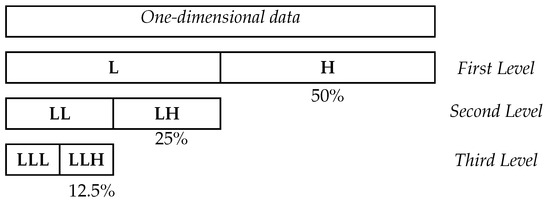
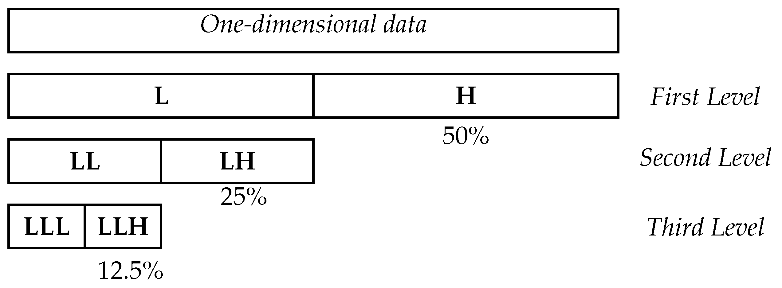
Figure 1 illustrates the PDWT with three decomposition levels. For , the sub-band L has low-pass wavelet coefficients (coarse information), whereas the sub-band H stores high-pass coefficients (detailed information). For , the second level is only applied to sub-band L, generating and sub-bands. For , the sub-band is transformed to obtain bands and , and so on, for further levels.
Figure 1.
PDWT with three levels: Analysis (top-down), synthesis (bottom-up).
For each level, , the number of low-pass wavelet coefficients L is reduced by half. The number of operations for convolution with the h and g filters is twice the length of data at the kth level, which has samples. Therefore, the complexity of the PDWT is , yielding an efficient linear complexity of .
The high-frequency components are in sub-bands with at least one H. The low-frequency sub-band contains only Ls. For two levels, the sub-band has low frequencies, and for three levels the sub-band has low frequencies as well. It is worth mentioning that the low-frequency sub-band preserves much of the energy, defined as the sum of the squares of the samples. Additionally, for a single transformation level (), erasing the H-band saves of the memory. For , erasing H and bands saves of the memory. For , erasing the H, , and bands saves of the memory, and so on. Although the reconstruction is not perfect, selecting a parametric filter can concentrate more energy in the low-frequency sub-band for the given samples [22], promoting a good approximation to perfect reconstruction.
| Algorithm 1 Parametric Discrete Wavelet Transform |
| Require: Signal array: data, Low-pass filter array of length FILTERSIZE: h, High-pass filter array of length FILTERSIZE: g, Number of wavelet decomposition levels: LEVELS |
| 1: procedure PDWT(data, data.length: n, FILTERSIZE, h, g, LEVELS) |
| 2: for to LEVELS do |
| 3: DWTlevel(data, data.length ≫ level, FILTERSIZE, h, g) |
| 4: end for |
| 5: end procedure |
| 6: procedure DWTlevel(data, data.length:n, FILTERSIZE, h, g) |
| 7: if then |
| 8: , |
| 9: tmp ← new array of size n ▹ Temporal array for wavelet coefficients |
| 10: for to step 2 do |
| 11: |
| 12: |
| 13: for to FILTERSIZE do |
| 14: ▹ Low frequency coefficients |
| 15: ▹ High frequency coefficients |
| 16: end for |
| 17: |
| 18: end for |
| 19: data ← tmp ▹ Updated wavelet coefficients |
| 20: end if |
| 21: end procedure |
For reconstruction (synthesis), the same number of levels must be applied as for PDWT. These levels correspond to the Parametric Inverse Discrete Wavelet Transform (PIDWT), which is described in Algorithm 2.
| Algorithm 2 Parametric Inverse Discrete Wavelet Transform |
| Require: Signal array: data, Low-pass filter array of length FILTERSIZE: Ih, High-pass filter array of length FILTERSIZE: Ig, Number of wavelet decomposition levels: LEVELS |
| 1: Ih, Ig ← InverseFilters(FILTERSIZE, h, g) |
| 2: procedure PIDWT(data, data.length: n, FILTERSIZE, Ih, Ig, LEVELS) |
| 3: for downto 0 do |
| 4: INVTWDLEVEL(data, data.length ≫ level, FILTERSIZE, h, g) |
| 5: end for |
| 6: end procedure |
| 7: procedure INVTWDLEVEL(data, data.length, FILTERSIZE, Ih, Ig) |
| 8: if then |
| 9: |
| 10: |
| 11: |
| 12: for to do |
| 13: |
| 14: for to do |
| 15: |
| 16: |
| 17: |
| 18: |
| 19: end for |
| 20: |
| 21: |
| 22: for to step 2 do |
| 23: |
| 24: |
| 25: end for |
| 26: |
| 27: end for |
| 28: |
| 29: end if |
| 30: end procedure |
For each transformation level the number of wavelet coefficients is duplicated up to the original via the PIDWT using two reconstruction filters and obtained from h and g, according to Algorithm 3.
| Algorithm 3 Reconstruction filters |
| 1: function InverseFilters() |
| 2: for to do |
| 3: |
| 4: |
| 5: |
| 6: end for |
| 7: return , |
| 8: end function |
The shortest filter has a length of two and corresponds to the Haar filter. Parametric length-four filters are shown in Equation (19).
Length-sixth filters are described in Equation (20), depending on two parameters and as follows:
It is worth mentioning that special cases for Equation (19) are Haar and Dau4, as is shown in Table 1, with the corresponding parameter [23].
Table 1.
Special cases for length-four parametric filters.
Additionally, there are special cases of length-sixth parametric filters of Equation (20) for Haar, Dau4, Dau6, and Coiflets, which are listed in Table 2 with the corresponding and parameters [23].
Table 2.
Special cases for length-sixth parametric filters.
By selecting one of these parameterizations for the low-pass h and high-pass g filters, the parametric discrete wavelet transform can be applied to the gradients of the Adam optimizer.
2.2. Fractional Derivatives and the Backpropagation Update Formula for MLP
There is no single definition of fractional derivatives. Three notable examples are the Grünwald–Letnikov, the Riemann–Liouville, and the Caputo fractional derivatives [16,19,24] which are defined and described briefly below.
Definition 1.
The Grünwald–Letnikov derivative with order of a given function is defined as:
Definition 2.
The Riemann–Liouville derivative with order and of a given function is defined as:
Definition 3.
The Caputo fractional derivative, for , and , is defined as:
Although these fractional derivatives are certainly related, they are not equivalent [25]. For example, the Riemann–Liouville definition is related to the Caputo definition as follows:
and, for a suitably smooth function , i.e., , then
From the definition of the Riemann–Liouville derivative, it follows that if is a non-zero constant, then:
which is not zero and is different from the integer case.
In this paper and other works, the Caputo definition is preferable to the Grünwald–Letnikov and Riemman–Liouville definitions because the Caputo fractional derivative of Equation (23) is zero for , with . This matches the integer derivative version [18].
Based on the previous discussion, we use the Caputo derivative definition to obtain a fractional expression for the gradients of the Adam algorithm. As we pointed out, the Caputo derivative of a constant is zero and for [18,26]:
In the case of , it yields to:
Given this fractional derivative and the backpropagation formula which is used to update the parameters of the Multilayer Perceptron (MLP) [1]:
our fractional version to update the gradients for FAdamWav is:
See Appendix A for details. Now, it is worth making a comment in this regard. In the context of the calculus of paradifferential operators in Sobolev spaces, and in this case for the Fourier multiplier operator , defined by:
the fractional chain rule [27,28] should be:
where E is an error as per the result of Christ and Weinstein [29]. Thus, by assuming , it is an approximation, useful for our purposes. Suppose that , , , . If , , and , then , and .
It is important to note that Equation (30) is the fractional version of Equation (A5), only different by the factor which is obtained when Equation (28) is applied to . Indeed, if , Equation (30) becomes the classical integer case. Then, Equation (30) represents a gradient-descent generalization with fractional order .
In practice, it is necessary to avoid two conditions:
- When the synaptic weights are zero, that yields to the indetermination of for .
- When is rational, we let and s is even (for example and ). Then, if , complex values are generated.
These situations have been previously studied in [20] and a solution consists of replacing by , for . In this way, the fractional gradient factor is defined as:
and the limit exists, and is equal to 1, for as .
With this consideration, Equation (30) becomes:
which generalizes the integer gradient-descent update rule, and it allows to compute the fractional gradient for the Adam optimizer by including the factor .
The following Algorithm 4 presents the FAdamWav steps. In this case, the gradient is a bidimensional matrix. In Step 1, the fractional gradient is obtained by applying Equation (34). To warrant a two-power for the n-dimension, zero padding is applied to obtain samples. Then, the PDWT is applied to m-tensors and therefore the computational complexity to calculate the PDWT is .
In this paper, it is meaningless to assume that a 2D wavelet transform on could be better to exploit some kind of “curves” inside . Instead, we just consider m transformations on n-dimensional tensors. However, we mention in brief a 2D approach, where a PWDT could be applied in two separated dimensions through tensor products of parametric filters or from non-tensor product of wavelet filters [30]. Indeed, it is possible to consider curvelets [31] and shearlets [32]. Curvelets are efficient transforms designed to work on images with edges along smooth curves, and they extend wavelets by incorporating directional selectivity and anisotropic scaling. The shearlet transform was designed to capture anisotropic features (like edges) in multidimensional data. We remark that these approaches are not considered in this paper, but it could be explored in future work.
Continuing with the FAdamWav algorithm (Algorithm 4), Step 5 shows which represents the low-frequency band (only “L’s”) along T iterations and the sub-bands with high-frequency components, for k transformation levels on . After applying the PDWT, the sub-bands are erased to save memory. Then, the and matrices are initialized to zero, and they are updated with in Steps 10 and 11, by considering Equations (8) and (9), respectively. has dimension of and and also save space since they have the same dimension. reduces the low-frequency coefficients by half for each level. For example, when , the memory of the fractional gradients is reduced by , has a dimension , and is set to zero in Step 6. So, in Step 12, is calculated using Equation (10) according to Adam’s update formula. One difference from related work [9] is that our algorithm fully erases and is not scaled by the formula which scales the high-frequency sub-bands with the matrix to deal with noisy gradients. In our research, we assume the existence of an optimal parametric filter to compress the gradients, allowing for non-perfect reconstruction of to update parameters, as shown in Step 15. The main idea is that it is possible to achieve a competitive accuracy relative to the original saving memory.
| Algorithm 4 FAdamWav: Fractional Adam with Wavelet Transform |
| Require: Weight matrix W, learning rate , batch size m. Adam decay rates . Iteration T. . Scale factor . Lowpass wavelet filter h, highpass wavelet filter g, Levels k. |
| 1: Initialize |
| 2: repeat |
| 3: ▹ Fractional gradient. See Equation (34) |
| 4: ▹ Save original length. Length() |
| 5: ▹ Gradient PDWT- Analysis |
| 6: ▹ No longer used, memory reduction |
| 7: if then |
| 8: Initialize |
| 9: end if |
| 10: |
| 11: |
| 12: ▹ was set to zero. Update rule, see Equation (10) |
| 13: ▹ PIDWT - Synthesis. Back to the original length |
| 14: ▹ Bias correction |
| 15: ▹ Update weights. Original dimensions for fractional gradients. |
| 16: |
| 17: until |
| 18: return |
Based on the previous concepts and Algorithm 4, the original PyTorch code for the Adam class [33] can be modified to obtain our fractional FAdamWav class, which is described in Listing 1. Specifically, by inserting Lines 8 to 20 as follows:
| Listing 1. FAdamWav Class: PyTorch Source Code |
|
1 class FAdamWav(Optimizer): 2 def step(self, closure: Callable = None): 3 … 4 for group in self.param_groups: 5 for p in group["params"]: 6 … 7 grad = p.grad 8 grad *= torch.pow(abs(grad)+ epsilon, 1-nu ) 9 grad /= torch.exp(torch.lgamma(torch.tensor( 2.0-nu ) )) 10 gr, original_lengths = pad_batch_to_pow2(grad) 11 pwt = ParametricWaveletTransform () 12 gr = pwt.PDWT(gr, len(gr)) 13 gr = gr[…, :gr.shape[−1] // 2] 14 grad = gr 15 … 16 gr = norm_grad 17 gr = duplicate_with_zeros(gr) 18 gr = pwt.PIDWT(gr, len(gr)) 19 gr = restore_original_lengths(gr, original_lengths) 20 grad = gr.squeeze(0) 21 norm_grad = grad |
In this case, the fractional factor depending of the -order is applied to (see Lines 8 and 9), and consequently it becomes a fractional gradient. (The source code for FAdamWav, PDWT, and PIDWT is available at http://ia.azc.uam.mx/sourcecode) (accessed on 23 February 2026).
In the same code, Lines 10 to 20 apply the parametric discrete wavelet transform. Line 12 applies the PDWT. Note that Line 13 considers low-pass wavelet coefficients exclusively, under the principle that these coefficients should concentrate much of the gradient energy (high-pass wavelet coefficients are neglected) which reduces the memory required for the gradients as previously explained. In Line 17, after using the gradients to update the synaptic weights, the high-pass wavelet coefficients are set to zero, and the PIDWT is applied in Line 18. Of course, this produces a non-perfect reconstruction, but it is sufficient to update the gradients of Adam since and are updated efficiently in the transformed space. The accuracy of the neural network should be lower than using the original gradient . However, the main idea is to maintain competitiveness while saving memory. This idea is supported by experimental results.
3. Results
This section describes four experiments that support the conclusions.
- Experiment 1. (FAdam). It explores the accuracy of a neural network with the following architecture:
- Linear(784, 64)
- ReLU()
- Linear(64, 10)
and fractional gradients on the MNIST dataset [34], without applying the parametric discrete wavelet transform. The neural network architecture is enough to match the input size of MNIST images ( pixels) and the output with 10 classes. The MNIST dataset has 60,000 images, divided into a training set of 50,000 and a test set of 10,000. - Experiment 2. (FAdamWav: Length-four filters). Given the same neural network and dataset as in Experiment 1, the second experiment applies the parametric wavelet transform to reduce the FAdam gradient memory by half by considering only the low-pass coefficients and a single transformation level. Several length-four parametric filters are tested varying the parameter for . In this case, the best -value from Experiment 1 is chosen (see below ).
- Experiment 3. (FAdamWav: Length-sixth filters). This experiment is similar to Experiment 2, but it considers length-sixth filters of Equation (20) depending on and . Each parameter independently takes on values equal to , where .
- Experiment 4. (FAdam, FAdamWav_k1, FAdamWav_k2, FAdamWav_k3). This experiment measures and compares the amount of GPU memory required for Adam and FAdamWav applying wavelet transformation levels. The execution time is also compared.
3.1. Experiment 1
Table 3 shows the accuracy of the neural network trained using FAdam and different fractional gradients , with step along 20 epochs. The maximum accuracy of is reached with , which is highlighted in bold.
Table 3.
Neural Network accuracy for different -values with the FAdam optimizer.
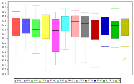
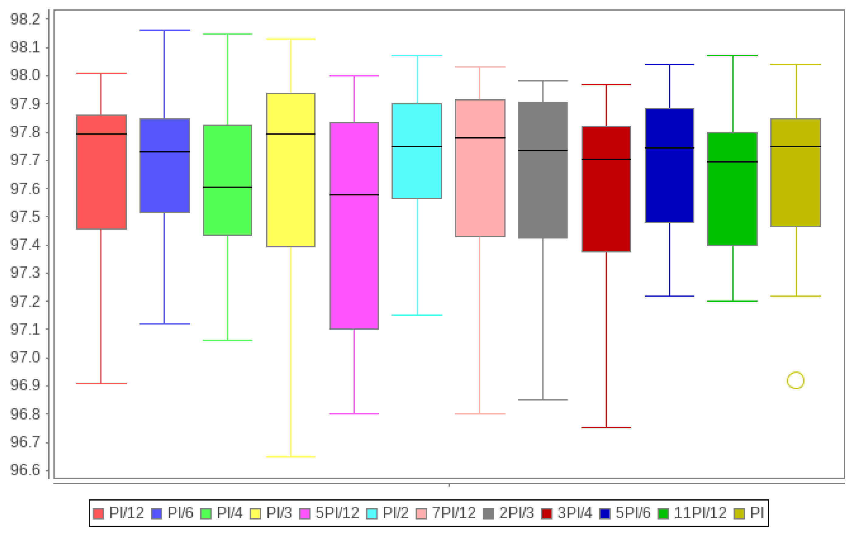
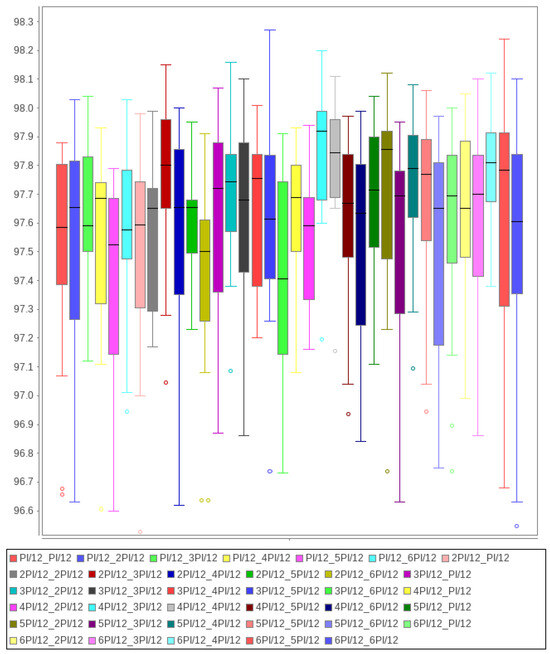
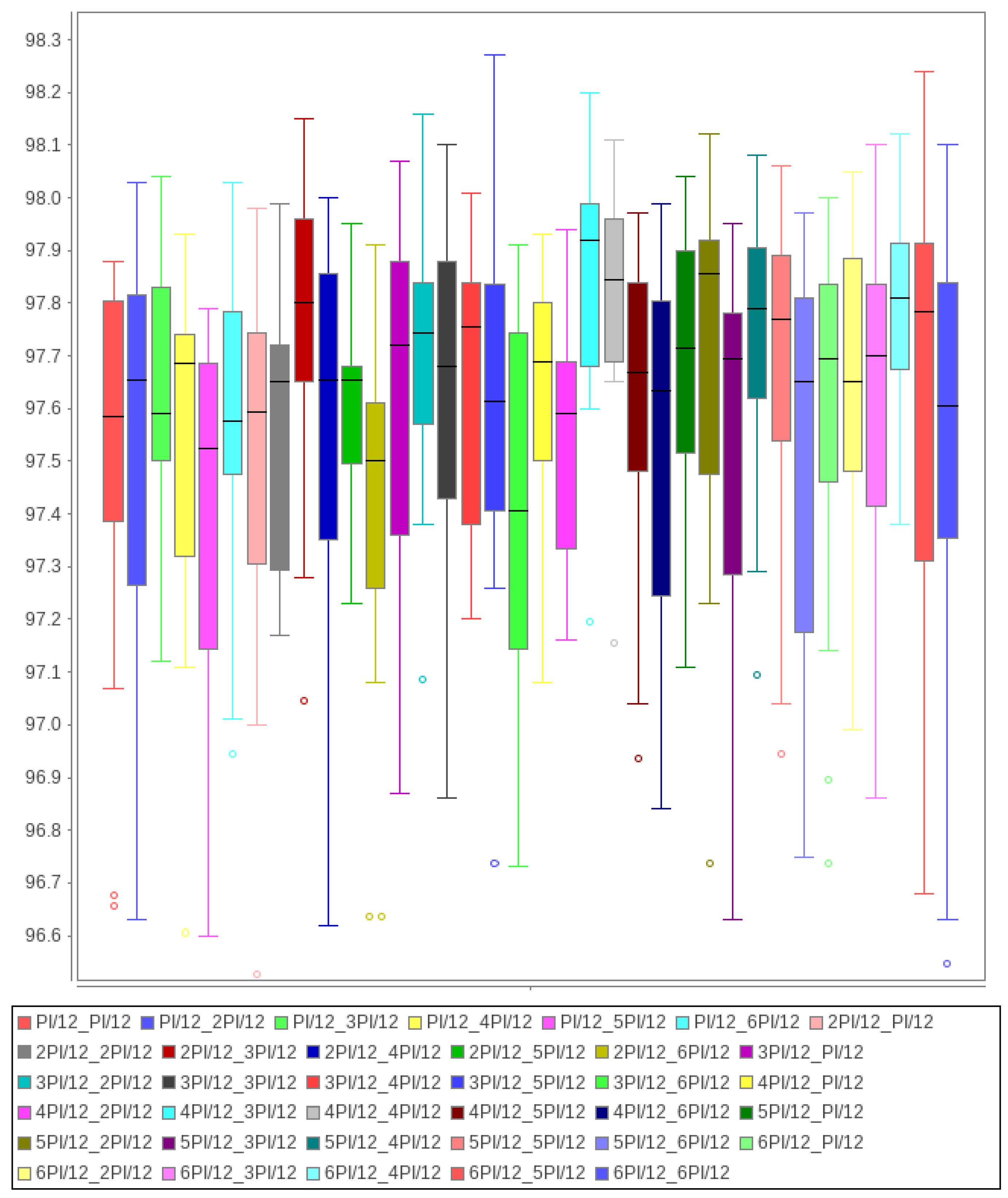
Figure 2 shows boxplots of the accuracies of Experiment 1 (with a step size of 0.1 for ), showing that the best performance is achieved with . Additionally, the plot shows that the integer case has lower performance than several fractional cases, including the case .
Figure 2.
FAdamWav accuracies for without PDWT.
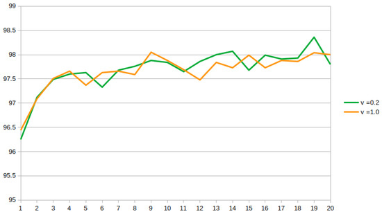
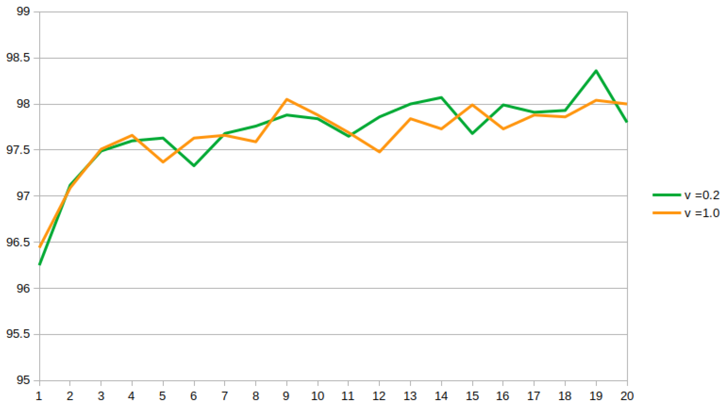
To complete Experiment 1, Figure 3 compares the performance of the integer case against the case . It is notorious that the fractional gradient reaches a higher accuraccy than the integer gradient.
Figure 3.
FAdam’s accuracy for (green) vs. (orange).
3.2. Experiment 2
The second experiment applies a single level of the parametric wavelet transform to reduce the FAdam gradient memory by half and by considering only the low-pass wavelet coefficients. Then, the gradients are updated, the high-pass coefficients are set to zero, and the parametric inverse wavelet transform is calculated to recover the original size of the Adam gradients.
Several length-four parametric filters were tested by varying the parameter for . The -value was fixed to . The corresponding accuracies are shown in columns of Table 4, where the highest accuracy was achieved with and is highlighted in bold.
Table 4.
Neural Network accuracy for with FAdamWav optimizer: Several values.
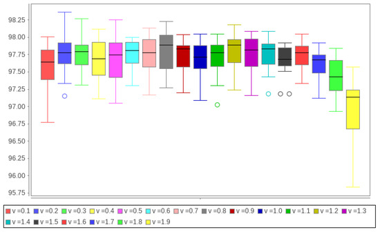
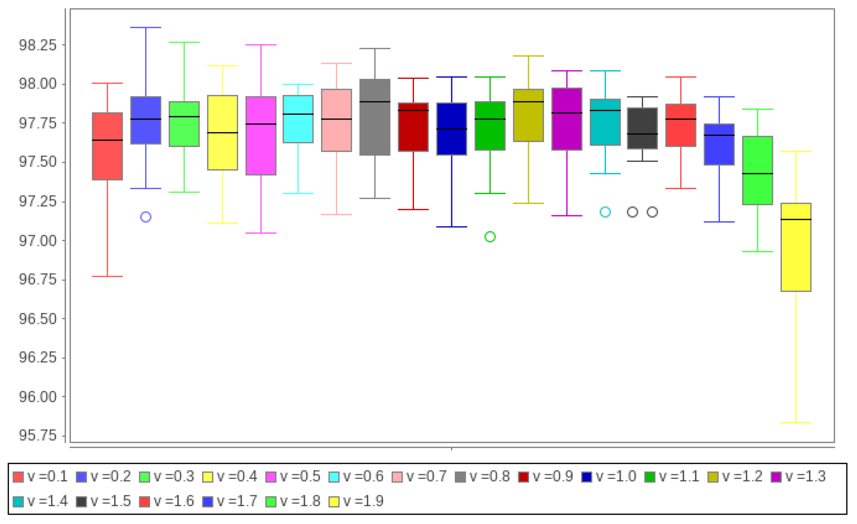
Figure 4 shows the boxplots of Table 4, and effectively it illustrates that the best performance occurs at .
Figure 4.
FAdamWav with length four filters, with .
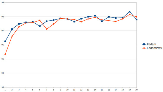
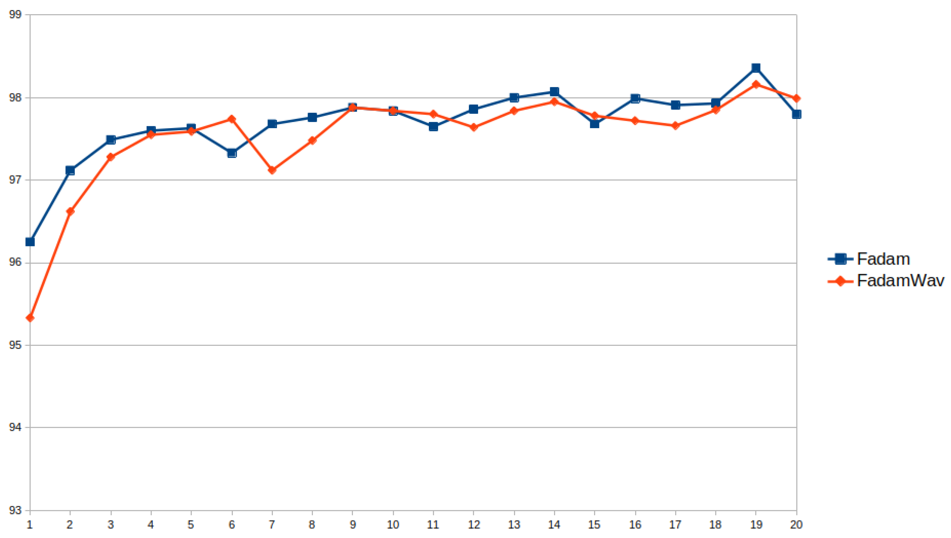
Figure 5 compares the accuracies of Fractional Adam (FAdam) with and Fractional Adam with parametric wavelet transform (FAdamWav) with and a parametric filter with . Although FAdam has a slightly better performance than FAdamWav, performance is still competitive but the memory required by the gradients is reduced by half.
Figure 5.
FAdam vs. FAdamWav with PDWT, length-four filters and .
3.3. Experiment 3
Experiment 3 considers FAdamWav with fractional order and the parametric length-sixth filters given in Equation (20) depending on and . In the experiment, and with .
The experiments were developed in PyTorch 2.3.1, running on a GPU NVIDIA GeForce RTX 3070. The Adam optimizer used a learning rate and the test accuracy was used as the metric for comparison.
Figure 6 shows the accuracy of each parametric filter (). The best result is for and . The experiment reveals that the filter modifies the training performance of the neural network.
Figure 6.
FAdamWav with length sixth filters, and equal to , for .
3.4. Experiment 4
In Experiment 4, the amount of GPU memory used during executions was measured. These executions developed a comparison with and without applying the wavelet transform: “FAdam” refers to the execution without wavelets whereas “FadamWav_k1”, “FAdamWav_k2”, “FAdamWav_k3” correspond to , and 3 wavelet transformation levels, respectively.
Note that theoretically, the memory savings are for FAdamWav_k1, for FAdamWav_k2, and for FAdamWav_k3. However, as shown in Table 5, the reduction in GPU memory using wavelets does not correspond to these percentages when compared to FAdam as the reference.
Table 5.
Gradient memory usage: FAdam vs. FAdamWav for , and 3 wavelet transformation levels.
Nevertheless, there is a reduction in GPU memory usage: from MB with FAdam to MB with FAdamWav_k1, which represents a reduction. A second transformation level reduces the GPU memory usage from MB to MB (a reduction). With three transformation levels, the memory usage remains at MB. Therefore, there is no further savings from two to three transformation levels. This is because GPU memory is assigned in blocks, so when memory usage does not change considerably, the reported memory usage remains the same.
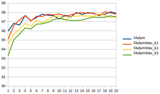
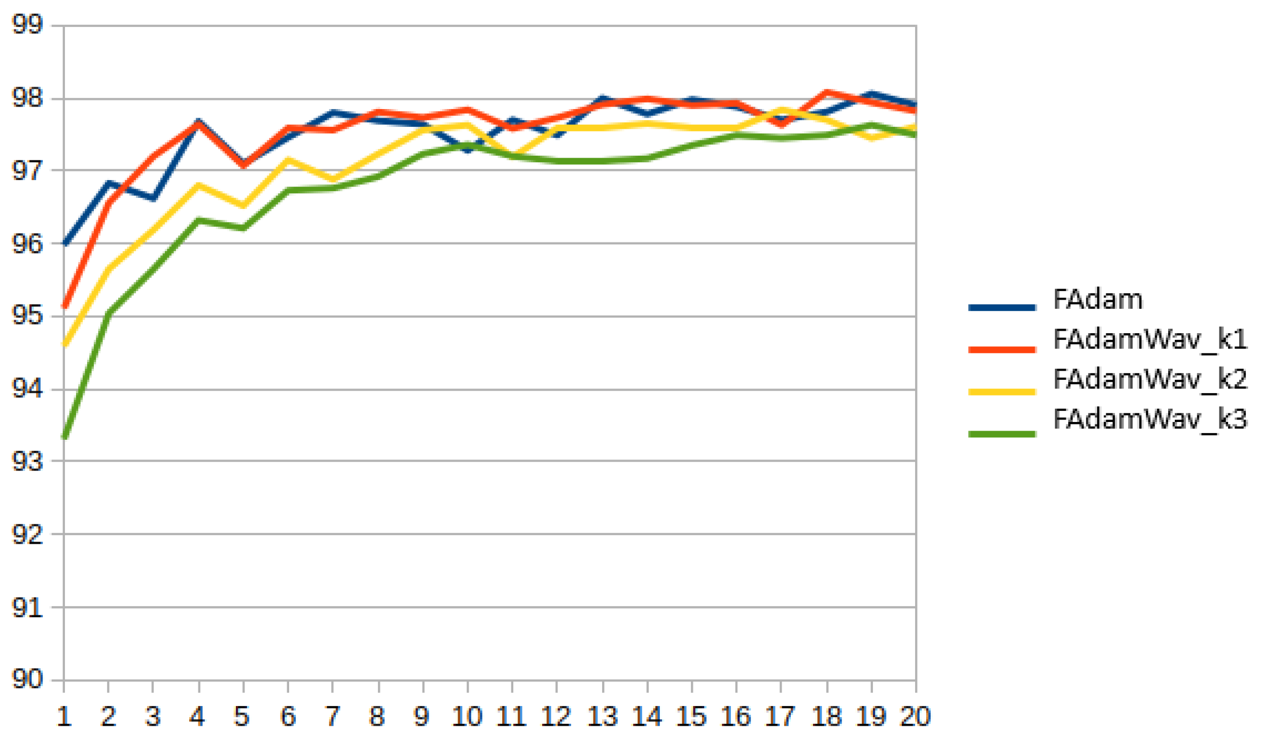
Figure 7 shows the accuracy for FAdam (without applying wavelets), FAdamWav_k1, FAdamWav_k2, and FAdamWav_k3, during 20 epochs. In Figure 7, it is possible to appreciate that:
Figure 7.
Adam vs. FAdamWav , and 3 transformation levels.
- FAdamWav_Level1 has a similar performance compared to FAdam, even though FAdamWav_Level1 saves of GPU memory.
- FAdamWav_Level2 has lower accuracy than FAdam and FAdamWav_k1, but it is still competitive despite the reduction in GPU memory.
- FAdamWav_Level3 has lower performance than FAdamWav_Level2, and no more GPU memory reduction.
The accuracies for FAdam, FAdamWav_k1, FAdamWav_k2, and FAdamWav_k3 are shown in Table 6.
Table 6.
Accuracy: Fadam vs. FadamWav for , and 3 wavelet transformation levels.
The elapsed time for the 20 epochs whose data are reported in Table 6 are shown in Table 7, where it is possible to see that:
Table 7.
Elapsed time: FAdam vs. FAdamWav for , and 3 wavelet transformation levels.
- The application of a single wavelet transformation level (FAdamWav_k1) increases the execution time for 50 s with respect to FAdam.
- The application of a second wavelet transformation level (FAdamWav_k2) increses the execution time for 70 s with respect to FAdam.
- The application of a third wavelet transformation level (FAdamWav_k3) increses the execution time to 94 s with respect to FAdam.
These experiments suggest that applying one or two transformation levels reduces GPU memory while maintaining competitive performance. However, using more than two transformation levels is not beneficial because it increases the execution time without providing additional memory reduction.
4. Discussion
The optimizer is a crucial component of neural network training. Due to the rapid growth of Artificial Intelligence, several gradient-based optimizers have been proposed. The Adam optimizer is considered the state of the art in deep learning because it outperforms other optimizers by considering historical adaptations of the moments. However, a drawback is the cost of storing and computing these gradients.
In this regard, we present FAdamWav, a variant of Adam which combines wavelet-based gradient compression with fractional gradient optimization.
The main idea behind FAdamWav is to reduce the memory required for the gradients by compressing them with a discrete wavelet transform while maintaining competitive accuracy. It also aims to improve performance by leveraging the fact that the fractional gradient optimizer outperforms the integer case. The integer case is a special case of the fractional optimizer when .
FAdamWav is characterized by the following:
- 1.
- Wavelet gradient compression. A wavelet-based gradient compression maps the gradient matrix to a reduced space via the parametric discrete wavelet transform with k transformation levels.
- 2.
- Efficient calculation of moments and velocities. Calculating the moments and velocities is efficient because high-frequency bands are removed in the wavelet low-dimensional space. Therefore, the gradients do not contain high frequencies.
- 3.
- Fractional gradient optimization. The fractional -order of the optimizer is variable. Selecting the appropriate value of provides good optimization. Our experiments show that the integer case is not optimal, and that the fractional version outperforms it. For instance, in Experiment 1, the best fractional order was .
- 4.
- Parametric filter selection. FAdamWav allows to select optimal parameter values of the filters for the discrete wavelet transform. The goal is to achieve maximum compression so that, even when the high-frequency coefficients are set to zero, the reconstructed gradients are sufficiently similar to the original.Although the experiments were developed by varying the parameters step by step with discrete values in the range , it is possible to adjust the -order during execution.
- 5.
- Neural network parameter optimization. The inverse parametric discrete wavelet transform restores the gradients to their original dimensions. Once restored, the gradients are used to update the network parameters for each training step.
- 6.
- Wavelet transformation levels. FAdamWav has the possibility of applying k transformation levels, and it is possible to choose a value of k that provides an acceptable trade-off between longer execution time and lower memory usage.
- 7.
- One-dimensional discrete wavelet transform. The discrete wavelet transform is applied in one dimension. However, it is possible to deal with the gradient matrix using a two dimensional wavelet transform, including curvelets or shearlets.
As previously mentioned, introducing the wavelet transform increases execution time, but this is an acceptable trade-off given the memory reduction.
Although the memory savings do not reach the theoretical limits of or for one and two transformation levels, the practical measurement of memory savings on the GPU is acceptable and supports the main idea behind FAdamWav.
From the experiments, it has been observed that considerable memory savings are achieved with one or two wavelet transformation levels. However, applying more than two transformation levels is not recommended. In fact, Experiment 4 shows that using three levels of the wavelet transform significantly increases execution time without reducing the amount of GPU memory.
In Experiment 2, the filters are first calculated based on the parameters, and then the DWT is applied. It is important to note that these parameters can be adjusted during training. Specifically, the parameter selection comes from a finite set of values in the range . However, the filters can be modified during execution.
Our experiments only consider small models. However, it is reasonable to expect that the main idea of FAdamWav applies to more complex models such as Large Language Models (LLMs) or Convolutional Neural Networks (CNNs), which require a lot of memory. LLMs are trained on massive amounts of text data, such as ChatGPT [35], Gemini [36], or LLaMA [37], and represent a memory challenge for training. CNNs [38] are models designed to process grid-like data, such as images, for tasks like image classification, object detection, and facial recognition. When training a CNN, memory is consumed not only by the parameters but also by the gradients. Thus, they also represents a challenge for training.
In this sense, memory reduction is still an open research area, and we contribute with FAdamWav.
Our study reveals a trade-off between the execution time, the neural network accuracy, the memory reduction, and the number k of transformation levels. The experiments demonstrate this relationship and encourage further research.
Finally, based on the previous discussion, we conclude that is possible to reduce the memory required by Adam’s gradients while maintaining a comparable performance to non-wavelet versions. Additionally, different parametric filters modify the training performance of a neural network, and there exists an optimal number of transformation levels that promotes the memory saving, good execution time and competitive accuracy.
Future work will focus on studying the automatic adaptation of parametric filters, the fractional order derivative, and the number of wavelet transformation levels.
Author Contributions
Conceptualization, O.H.-A., S.A.-B., and J.N.-F.; Methodology, O.H.-A., S.A.-B., J.N.-F., S.R.-M., and J.A.R.-O.; Software, O.H.-A., J.A.R.-O., and S.R.-M.; Validation, O.H.-A., S.A.-B., S.R.-M., J.A.R.-O., and J.N.-F.; Writing—review and editing, O.H.-A., S.A.-B., S.R.-M., J.A.R.-O., and J.N.-F. All authors have read and agreed to the published version of the manuscript.
Funding
This research received no external funding.
Data Availability Statement
The original contributions presented in the study are included in the article, further inquiries can be directed to the corresponding author.
Conflicts of Interest
The authors declare no conflict of interest.
Appendix A. Fractional Derivatives and the Backpropagation Update Formula for MLP
We let a training set with N samples and a neural network architecture be described as follows:
- X is the input layer (input data),
- H is hidden layers,
- O is the output layer,
- L is layers, because of the hidden layers and the output layer,
- is a matrix of synaptic weights, , that connects neuron k of layer with neuron j of layer l,
- are synaptic weights () that connect the first hidden layer with X,
- is the desired output of neuron k at output layer when the ith input data is presented,
- is the activation function in the L layers,
- is the output of neuron k at output layer O, when the ith input data are presented and at layer O,
- is the potential activation of neuron k at layer l, , with inputs . For , considering the jth component of X,
- is the output of neuron k at a hidden layer l, .
Note that at the output layer, the error of neuron k is and the subindex i means that the ith input pattern is presented to the neural network.
For all the neurons, the error at the output layer is:
and the cumulative error of the N training samples is:
The backpropagation algorithm aims to find optimal values for the free parameters of the weight matrix that minimize E.
The optimization with the gradient-descent method applied to the weight updates is:
that points to the direction where decays. In this context, is the learning rate. Additionally, the local gradient is defined as:
and since
then, can be expressed as:
For , Equation (A4) becomes and then, at the output layer O:
For , the local gradient for hidden layers is:
and consequently, the weight updates are:
References
- Haykin, S.S. Neural Networks and Learning Machines, 3rd ed.; Pearson Education: Upper Saddle River, NJ, USA, 2009. [Google Scholar]
- Robbins, H.; Monro, S. A stochastic approximation method. Ann. Math. Statist. 1951, 22, 400–407. [Google Scholar] [CrossRef] [Scilit]
- Lydia, A.; Francis, S. Adagrad—An Optimizer for Stochastic Gradient Descent. Int. J. Inf. Comput. Sci. 2019, 6, 566–568. [Google Scholar]
- Zeiler, M. ADADELTA: An adaptive learning rate method. arXiv 2012, arXiv:1212.5701. [Google Scholar] [CrossRef] [Scilit]
- Kingma, D.P.; Ba, J. Adam: A Method for Stochastic Optimization. arXiv 2014, arXiv:1412.6980. [Google Scholar]
- Hu, E.J.; Shen, Y.; Wallis, P.; Allen-Zhu, Z.; Li, Y.; Wang, S.; Wang, L.; Chen, W. LoRA: Low-Rank Adaptation of Large Language Models. arXiv 2021, arXiv:2106.09685. [Google Scholar] [CrossRef] [Scilit]
- Zhao, J.; Zhang, Z.; Chen, B.; Wang, Z.; Anandkumar, A.; Tian, Y. Galore: Memory-efficient LLM Training by Gradient Low-rank Projection. arXiv 2024, arXiv:2403.03507. [Google Scholar] [CrossRef] [Scilit]
- Wang, Y.; Yang, Z.; Chen, B.K.; Pu, F.; Li, B.; Gao, T.; Kawaguchi, K. Memory-Efficient LLM Training by Various-Grained Low-Rank Projection of Gradients. arXiv 2025, arXiv:2505.01744. [Google Scholar]
- Wen, Z.; Luo, P.; Wang, J.; Deng, X.; Zou, J.; Yuan, K.; Sun, T.; Li, D. Wavelet Meets Adam: Compressing Gradients for Memory-Efficient Training. arXiv 2025, arXiv:2501.07237. [Google Scholar]
- Daubechies, I. Ten Lectures on Wavelets; Society for Industrial and Applied Mathematics (SIAM): Philadelphia, PA, USA, 1992. [Google Scholar]
- Mallat, S. A Wavelet Tour of Signal Processing: The Sparse Way, 3rd ed.; Academic Press, Inc.: Cambridge, MA, USA, 2008. [Google Scholar]
- Herrera Alcántara, O.; González Mendoza, M. Optimization of Parameterized Compactly Supported Orthogonal Wavelets for Data Compression. In Proceedings of the Advances in Soft Computing; Batyrshin, I., Sidorov, G., Eds.; Springer: Berlin/Heidelberg, Germany, 2011; pp. 510–521. [Google Scholar]
- Lai, M.J.; Roach, D. Parameterizations of Univariate Orthogonal Wavelets With Short Support. In Approximation Theory X: Wavelets, Splines, and Applications; Chui, C.K., Schumaker, L.L., Stoeckler, J., Eds.; Vanderbilt University Press: Nashville, TN, USA, 2001; pp. 1–10. [Google Scholar]
- Roach, D.W. A Subclass of the Length 12 Parameterized Wavelets. In Proceedings of the Approximation Theory XIII: San Antonio 2010; Neamtu, M., Schumaker, L., Eds.; Springer: New York, NY, USA, 2012; pp. 263–275. [Google Scholar]
- Roach, D. The complete length sixteen parametrized wavelets. Sampl. Theory Signal Process. Data Anal. 2025, 23, 12. [Google Scholar] [CrossRef] [Scilit]
- Podlubny, I. Chapter 2—Fractional Derivatives and Integrals. In Fractional Differential Equations;Mathematics in Science and Engineering; Podlubny, I., Ed.; Elsevier: Amsterdam, The Netherlands, 1999; Volume 198, pp. 41–119. [Google Scholar] [CrossRef] [Scilit]
- Miller, K.S.; Ross, B. An Introduction to the Fractional Calculus and Fractional Differential Equations; Wiley-Interscience: Hoboken, NJ, USA, 1993. [Google Scholar]
- Bao, C.; Pu, Y.; Zhang, Y. Fractional-Order Deep Backpropagation Neural Network. Comput. Intell. Neurosci. 2018, 2018, 7361628. [Google Scholar] [CrossRef] [Scilit] [PubMed]
- Wang, J.; Wen, Y.; Gou, Y.; Ye, Z.; Chen, H. Fractional-order gradient descent learning of BP neural networks with Caputo derivative. Neural Netw. 2017, 89, 19–30. [Google Scholar] [CrossRef] [Scilit] [PubMed]
- Herrera-Alcántara, O. Fractional Derivative Gradient-Based Optimizers for Neural Networks and Human Activity Recognition. Appl. Sci. 2022, 12, 9264. [Google Scholar] [CrossRef] [Scilit]
- Herrera-Alcántara, O.; Castelán-Aguilar, J.R. Fractional Gradient Optimizers for PyTorch: Enhancing GAN and BERT. Fractal Fract. 2023, 7, 500. [Google Scholar] [CrossRef] [Scilit]
- Herrera Alcántara, O. On the Best Evolutionary Wavelet Based Filter to Compress a Specific Signal. In Proceedings of the Advances in Soft Computing; Sidorov, G., Hernández Aguirre, A., Reyes García, C.A., Eds.; Springer: Berlin/Heidelberg, Germany, 2010; pp. 394–405. [Google Scholar]
- Herrera-Alcántara, O.; González-Mendoza, M. Inverse formulas of parameterized orthogonal wavelets. Comput. Informat. Numer. Comput. 2018, 100, 715–739. [Google Scholar] [CrossRef] [Scilit]
- Luchko, Y. Fractional Integrals and Derivatives: “True” versus “False”. Mathematics 2023, 11, 3003. [Google Scholar] [CrossRef] [Scilit]
- Wilson, H.; Sircar, S.; Shukla, P. Viscoelastic Subdiffusive Flows: Theory and Computation; Fluid Mechanics and Its Applications; Springer: Singapore, 2024; Volume 138. [Google Scholar] [CrossRef] [Scilit]
- Garrappa, R.; Kaslik, E.; Popolizio, M. Evaluation of Fractional Integrals and Derivatives of Elementary Functions: Overview and Tutorial. Mathematics 2019, 7, 407. [Google Scholar] [CrossRef] [Scilit]
- Taylor, M.E. Tools for PDE: Pseudodifferential Operators, Paradifferential Operators, and Layer Potentials; Mathematical Surveys and Monographs; American Mathematical Society: Providence, RI, USA, 2000; Volume 81. [Google Scholar]
- Bényi, Á.; Maldonado, D.; Naibo, V. What is… a paraproduct. Not. Am. Math. Soc. 2010, 57, 858–868. [Google Scholar]
- Christ, F.M.; Weinstein, M.I. Dispersion of small amplitude solutions of the generalized Korteweg-de Vries equation. J. Funct. Anal. 1991, 100, 87–109. [Google Scholar] [CrossRef] [Scilit]
- Conti, C.; Cotronei, M. Construction of Wavelet Filters: A Revisitation. In Proceedings of the Mathematical and Computational Modelling, Approximation and Simulation; Ibáñez-Pérez, M.J., Lamberti, P., Remogna, S., Sbibih, D., Eds.; Springer: Cham, Switzerland, 2025; pp. 3–21. [Google Scholar]
- Candes, E.J.; Donoho, D.L. Curvelets: A Surprisingly Effective Nonadaptive Representation for Objects with Edges. In Proceedings of the International Conference on Curves and Surfaces, Saint-Malo, France, 1–7 July 1999; pp. 1–10. [Google Scholar]
- Kutyniok, G.; Labate, D. (Eds.) Shearlets: Multiscale Analysis for Multivariate Data, 1st ed.; Applied and Numerical Harmonic Analysis; Springer: New York, Ny, USA, 2012; p. 345. [Google Scholar]
- Paszke, A.; Gross, S.; Massa, F.; Lerer, A.; Bradbury, J.; Chanan, G.; Killeen, T.; Lin, Z.; Gimelshein, N.; Antiga, L.; et al. PyTorch: An Imperative Style, High-Performance Deep Learning Library. In Advances in Neural Information Processing Systems 32; Curran Associates, Inc.: Red Hook, NY, USA, 2019; pp. 8024–8035. [Google Scholar]
- Deng, L. The MNIST database of handwritten digit images for machine learning research. IEEE Signal Process. Mag. 2012, 29, 141–142. [Google Scholar] [CrossRef] [Scilit]
- OpenAI. ChatGPT. Large Language Model. 2023. Available online: https://chat.openai.com/ (accessed on 23 February 2026).
- DeepMind, G. Gemini. Large Language Model Developed by Google DeepMind. 2023. Available online: https://deepmind.google/technologies/gemini/ (accessed on 23 February 2026).
- Grattafiori, A.; Dubey, A.; Jauhri, A.; Pandey, A.; Kadian, A.; Al-Dahle, A.; Letman, A.; Mathur, A.; Schelten, A.; Vaughan, A.; et al. The LLaMA 3 Herd of Models. arXiv 2024, arXiv:2407.21783. [Google Scholar] [CrossRef] [Scilit]
- Montesinos, L.O.A.; Montesinos, L.A.; Crossa, J. Convolutional Neural Networks. In Multivariate Statistical Machine Learning Methods for Genomic Prediction; Springer: Cham, Switzerland, 2022; pp. 533–577. [Google Scholar] [CrossRef] [Scilit]

Disclaimer/Publisher’s Note: The statements, opinions and data contained in all publications are solely those of the individual author(s) and contributor(s) and not of MDPI and/or the editor(s). MDPI and/or the editor(s) disclaim responsibility for any injury to people or property resulting from any ideas, methods, instructions or products referred to in the content. |
© 2026 by the authors. Licensee MDPI, Basel, Switzerland. This article is an open access article distributed under the terms and conditions of the Creative Commons Attribution (CC BY) license.