


Abstract
In current low-pressure turbine cascades, around a third of the losses are determined by the complex interaction between endwall boundary layers and blade profiles. Research has focused on the origin of secondary flow structures through numerical and experimental approaches, which shed light on vorticity transport throughout the cascades. This paper details the study of the endwall flow characteristics in the newly published open-access high-speed low-pressure turbine cascade SPLEEN. This study focuses on the effect of inlet turbulence profile specification, which is studied by computational fluid dynamics in design and off-design conditions. Numerical simulations are performed using transition-sensitive Reynolds-Averaged Navier–Stokes closures, which have proved to be a reliable tool for identifying secondary flow structures in similar configurations. In this activity, RANS-based transition models capture the secondary flow structure, but underestimate mixing and over-predict losses near the hub. Inlet turbulence profiles have little effect on endwall pressure, while higher turbulence intensity and integral length scales enhance secondary flow mixing, reduce vortex penetration, and increase hub losses. In off-design conditions, a low Mach number increases secondary flow penetration and endwall losses, whereas a high Reynolds number reduces both profile and endwall losses. Finally, selected correlations from the literature agree at the nominal Reynolds number but do not capture the variations across the various conditions explored.
1. Introduction
For axial turbomachinery, the endwall flow region can be the origin of 30–40% of overall losses ([1]), caused by viscous dissipation in the endwall boundary layer and mixing of secondary flows. The origin of secondary flow structures can be predicted by simplifying inviscid flow assumptions [2], in which the streamwise vorticity is generated through the bending and stretching of vortex filaments under the potential flow field imposed by the cascade, along with spanwise variation in blade circulation. Despite this, successive experimental and numerical work has suggested that the secondary flow pattern can be more complex than predicted by inviscid flow theory. A comprehensive description of the secondary vortex systems measured during early experimental campaigns is present in the paper by Sieverding [3]. The inlet endwall boundary layer separates under the pressure gradient imposed by the blade’s leading edge potential effect. This generates a so-called horseshoe vortex (HV) ([4]), characterized by two legs of opposite vorticity traveling across the passage ([5]). The pressure gradient in the cascade’s blade-to-blade plane pushes the pressure-side leg of the horseshoe vortex and low-momentum fluid in the endwall boundary layer towards the suction side, generating another vortical structure called passage vortex (PV). In some experimental research (e.g., Sieverding [6] and Wang et al. [7]), the suction-side leg of the HV migrates along the suction side, describing a helical motion around the PV. Sieverding acknowledges that the path of the suction-side leg with respect to the PV at the outlet plane is a function of blade characteristics and flow conditions. In [5], it was suggested that the suction-side leg remains confined to the endwall region, resulting in a region of opposite vorticity to the PV in the outlet plane. According to oil-flow visualizations by Hodson and Dominy [8], the strong interaction between leading edge-separation lines and the suction-side boundary layer can induce the presence of opposite vorticity to the passage vortex. The originating structure is typically called the corner vortex (CV).
Secondary flow topology is highly dependent on the blade design and inlet flow conditions. Recent studies have shed some light on the parameters influencing secondary flows and their associated losses. Hodson and Dominy [9] performed experiments varying the pitch-to-chord ratio of a low-pressure turbine (LPT) airfoil, concluding that the secondary losses increase with blade loading. Both Weiss and Fottner [10] and Benner et al. [11] studied the effect of loading distribution by varying the blade design and the stagger angle, respectively. Their results indicate that front-loaded designs feature higher secondary vorticity. Other researchers experimentally investigated the effect of the inlet boundary layer thickness, concluding that it has a low impact on the development of secondary losses (e.g., [12]). On the other hand, other studies have shown that uniform and realistic boundary layer profiles specified for a high-pressure turbine vane lead to significant discrepancies in the endwall flow ([13]). The effect of the inlet boundary layer shape factor was studied in [14]. The authors showed that laminar boundary layers are associated with stronger vorticity at the cascade outlet and more loss cores than turbulent boundary layers.
In modern high-speed engine environments, the development of these secondary structures is drastically altered by unsteady perturbations. Recent experimental and numerical investigation on the SPLEEN cascade have demonstrated that the injection of purge flow from hub cavities and the interaction with periodic upstream wakes tend to compress the passage and trailing shed vortices towards the endwall, significantly modifying the extension and the core of the aerodynamic losses [15,16,17]. The complex flow physics characterizing modern high-speed cascades, which involve bubbles, shock wave interactions, and transition mechanisms, have recently driven the community towards high-fidelity simulations, such as Direct Numerical Simulations (DNSs) and Wall-Resolved Large-Eddy Simulations (LESs) [18,19,20,21]. However, due to the prohibitive computational costs of these methods, Reynolds-Averaged Navier–Stokes (RANS) approaches remain an indispensable tool for industrial design, especially considering recent efforts to accurately predict the transition onset and separated bubble reattachment [22,23].
Due to increased computational power, this topic has recently been central to the numerical studies of low-pressure turbine blades. Ciorciari et al. [24] studied the effect of passing wakes on developing secondary flows in a linear turbine cascade. The authors showed that incoming wakes modify the structure of secondary flows, periodically reducing the strength of the PV, the CV, and the wake. High-fidelity simulations were used by Cui et al. [25] to compare cascade losses obtained with laminar, turbulent, and wake-induced inlet boundary layers. The authors concluded that the losses generated by a turbulent boundary layer and wake disturbance are higher than the laminar and undisturbed turbulent case. Giovannini et al. [26] studied both numerically and experimentally, hinting at the necessity of careful mesh definition over the endwall to avoid secondary flow distortion.
The effect of profile specification for the inlet boundary layer was studied using LESs and RANS simulations [27,28]. Among all, one of the conclusions of the authors was that the RANS and LES approaches yield very similar results, with minor differences present in the wake-development and endwall-flow structures, also highlighting that a careful specification of the boundary layer is necessary to achieve satisfactory predictions of the secondary flow system.
Coull [29] used RANS-based simulations to investigate the effect of blade design parameters on the losses associated with developing the endwall and secondary flows. Coull and Clark [30] investigated the impact of boundary layer thickness and shape factor on the secondary losses for a linear cascade, showing that the vorticity distribution of the inlet profile directly affects secondary flow structures. The effect of the turbulence level was instead studied in [31], where different inlet boundary layers were investigated experimentally and numerically for a subsonic Mach low-pressure turbine cascade. The authors numerically evidenced the inlet turbulence level specification’s effect in the boundary layer, concluding that higher turbulence intensity leads to a faster dissipation of secondary flow structures and, consequently, more pronounced losses close to the endwall.
In this paper, numerical simulations based on transition-sensitive RANS closures are adopted to gain further insights into the generation of secondary vorticity associated with different inlet turbulent quantity specifications in an axial low-pressure turbine cascade. The test case is the SPLEEN C1 blade, investigated at the von Karman Institute for Fluid Dynamics in the context of the EU-funded project SPLEEN. Different experimental inlet conditions are scrutinized in terms of predictions of loading, outlet losses, and endwall flows, which are thoroughly compared to experimental measurements for the design conditions of the cascade. Numerical and experimental results in off-design conditions allow the investigation of the effect of the isentropic Mach number and Reynolds number of the secondary flow field generated in engine-relevant configurations. This paper is organized as follows: in Section 2, the SPLEEN cascade is described along with the experimental methodology; in Section 3, the numerical approach is detailed, highlighting the specification of turbulence inlet quantities; Section 4 reports the analysis of the grid dependence, while Section 5 details the main findings of this paper, assessing the distribution of secondary flows and the impact of off-design conditions on the performance of the cascade.
2. Test Case Description
This study focuses on the endwall flow of a linear low-pressure turbine cascade experimentally investigated at the von Karman Institute for Fluid Dynamics (BE) in the context of the EU-funded project SPLEEN. The SPLEEN C1 blade represents a modern rotor airfoil for high-speed LPT. Table 1 reports the key geometrical characteristics of the airfoil and flow conditions at which the cascade was investigated.
Table 1.
SPLEEN C1 geometry.
The experimental campaign occurred in the VKI S-1/C high-speed, low-Reynolds closed-loop facility. A 13-stage axial compressor powers this rig, maintaining near-ambient temperature conditions through an air-to-oil heat exchanger. Control over the mass-flow rate in the loop is achieved by adjusting the compressor’s rotational speed and a bypass valve. The cascade, located in the first elbow of the closed loop downstream of the compressor, benefits from a wire mesh and honeycomb configuration to ensure homogeneous inlet flow conditions to the cascade test section.
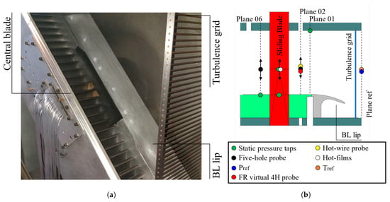
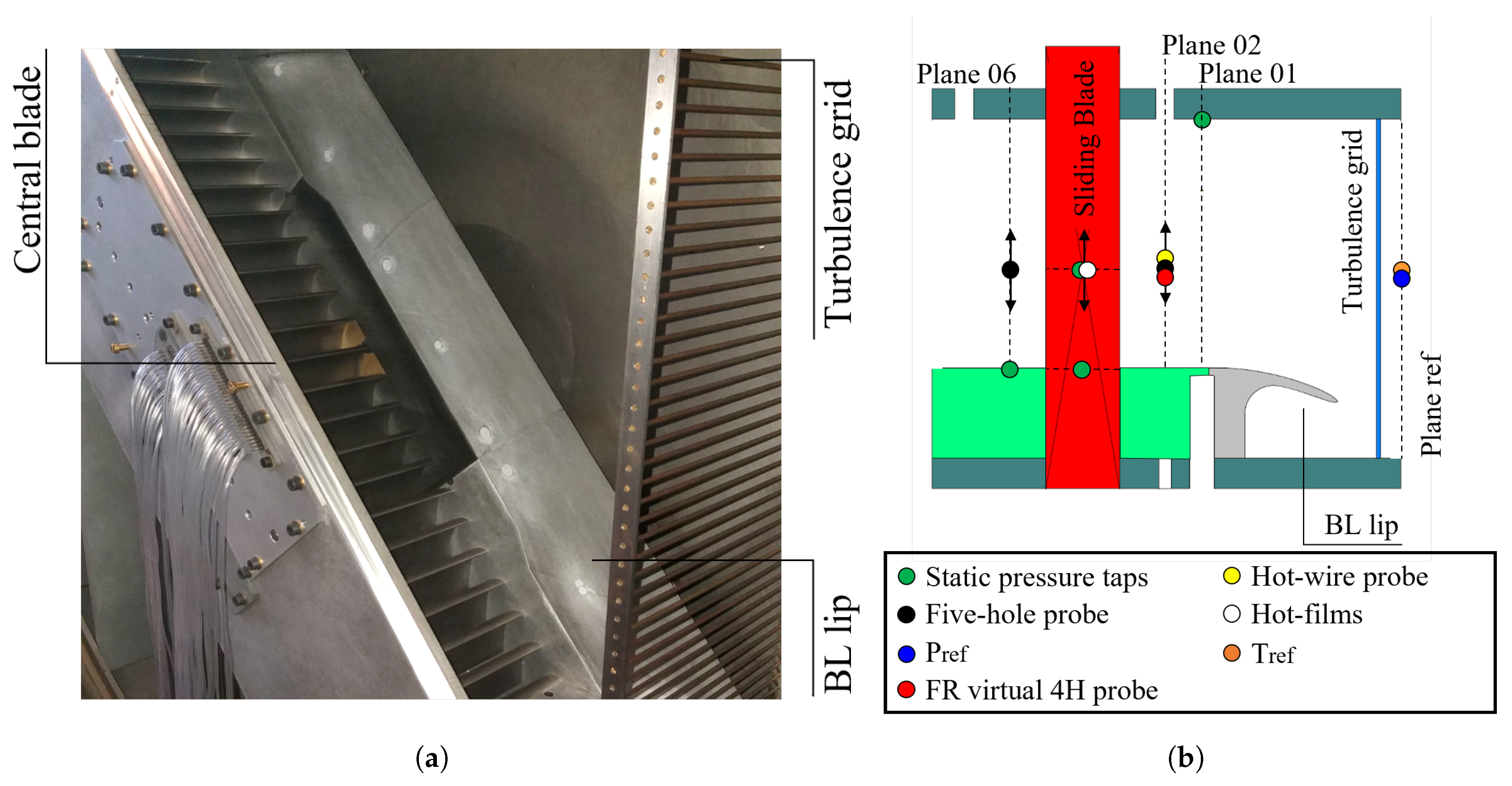
Figure 1a illustrates the cascade mounted in the first elbow of the VKI S-1/C, while Figure 1b provides a depiction of the cascade test section and the measurement planes used in this study. Since the cascade is extensively instrumented [32], only the instrumentation relevant to this study is presented, particularly highlighting the turbulence grid location.
Figure 1.
Experimental setup. (a) Linear cascade and constituents. (b) Meridional cut with location of measurement planes and instrumentation.
Fixed instrumentation is employed for real-time monitoring of flow conditions within the rig. The isentropic-outlet/inlet Mach number and Reynolds number are estimated using the inlet total pressure downstream of the grid, outlet/inlet static pressure, and inlet total temperature. Since the inlet total pressure is not directly measured, a correlation was developed to estimate the cascade’s total inlet pressure based on the measured reference total pressure upstream of the turbulence grid. It is important to note that for the cases analyzed here, according to Roach’s correlation [33], both turbulence intensity and integral length scale are insensitive to variations in the Reynolds number at the cascade outlet since the Reynolds number relative to the turbulence grid remains within the range . For further details about the test case, refer to [32].
The reference total pressure and temperature were obtained using an absolute pressure sensor (WIKA P-30) and a bare K-type thermocouple. Static pressure measurements were taken at Plane 01 (PL01) (1.12 upstream of the blade’s leading edge) and Plane 06 (PL06) (0.50 downstream of the blade’s trailing edge). Inlet turbulence measurements utilized two hot-wire probes operating in constant temperature mode. The inlet flow field at Plane 02 (PL02) (0.50 upstream of the blade’s leading edge) was characterized using a Cobra-shaped five-hole probe (C5HP), while the outlet flow field at PL06 was surveyed with an L-shaped five-hole probe (L5HP). The blade loading was computed from pressure tap measurements on the blade surface, with 24 taps on the suction side (SS) and 17 taps on the pressure side (PS). The taps were traversed at 46 points in the spanwise direction. The endwall static pressure was measured by merging the readings of 66 taps distributed between two inserts in adjacent passages. Pressure measurements from pneumatic probes and pressure taps at PL01, PL06, and blade surfaces were recorded using two Scanivalve MPS4264s with ranges of 1 psi and 2.5 psi. Turbulence measurements were performed with a single wire, and a fast-response aerodynamic probe was operated in virtual mode. Both of them were sampled with a 16-bit NI6253-USB card. The database does not report the uncertainty of the turbulent quantities retrieved with the fast-response probe. The uncertainty of the quantities computed with the instrumentation mentioned above is presented in Table 2. Both random and systematic uncertainties are expressed with a 95% confidence interval.
Table 2.
Experimental uncertainty.
A thorough description of the test case can be found in [32]. The experimental data used in this work has been previously presented in [34] and can be obtained from an open-access repository [35]. Furthermore, the accurate characterization of the inlet turbulence level in compressible and rarefied regimes using hot-wire anemometry [36] and Background-Oriented Schlieren (BOS) [37] makes it an ideal test to evaluate the sensitivity of turbulence models.
3. Numerical Methodology
All the simulations were run using the in-house solver HybFlow, developed at the Politecnico di Torino and validated against experimental data for the evaluation of compressible flows in turbomachinery [38,39]. The code is based on a cell-centered finite volume method, solving the Navier–Stokes equations in the conservative form on hybrid grids [40,41]. Inviscid fluxes are discretized using Roe’s scheme [42], while viscous flux computation is based on a central difference scheme. The code achieves second-order accuracy, employing a least-square variable reconstruction based on the approach proposed in [43,44]. Turbulent fluxes are based on a second-order upwind scheme. A steady solution is achieved using a numerical time-stepping technique, with constant CFL = 5.0. The solution is considered as converged when the residuals for all the equations reach a threshold level equal to with a mass-flow imbalance below .
All computations are based on the RANS approach to close the turbulence problem. The SST model by [45], in combination with the transition model [46,47], was employed to account for turbulence effects. Air is treated as an ideal gas characterized by a constant molecular viscosity value of kg/(m·s), a thermal conductivity W/(m·K), Prandtl number , and turbulent Prandtl number .
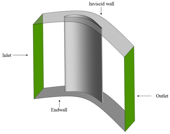
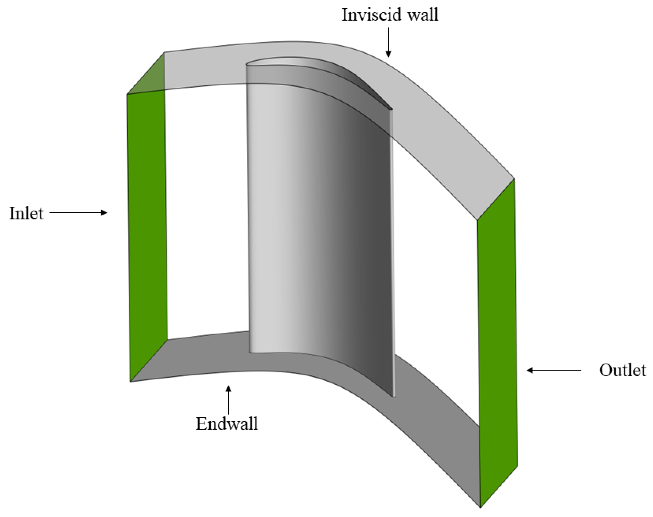
The domain used for the present calculation is shown in Figure 2. The domain extends from the lower endwall to the mid-span of the cascade, where an inviscid wall is used to simulate symmetry conditions. Lateral boundaries are instead periodic. Viscous walls are set as adiabatic. The inlet of the domain corresponds to PL02 to correctly impose experimentally measured inlet conditions to the cascade. The outlet of the domain is placed 1.0 downstream of the trailing edge.
Figure 2.
Numerical domain.
A validation of the solver is present in [47]. Three different simulations were run in the present activity, as reported in Table 3. Nominal conditions were used as a reference to study the impact of spatial discretization of the domain and the definition of the inlet boundary layer coming from the experimental measurements.
Table 3.
Test matrix.
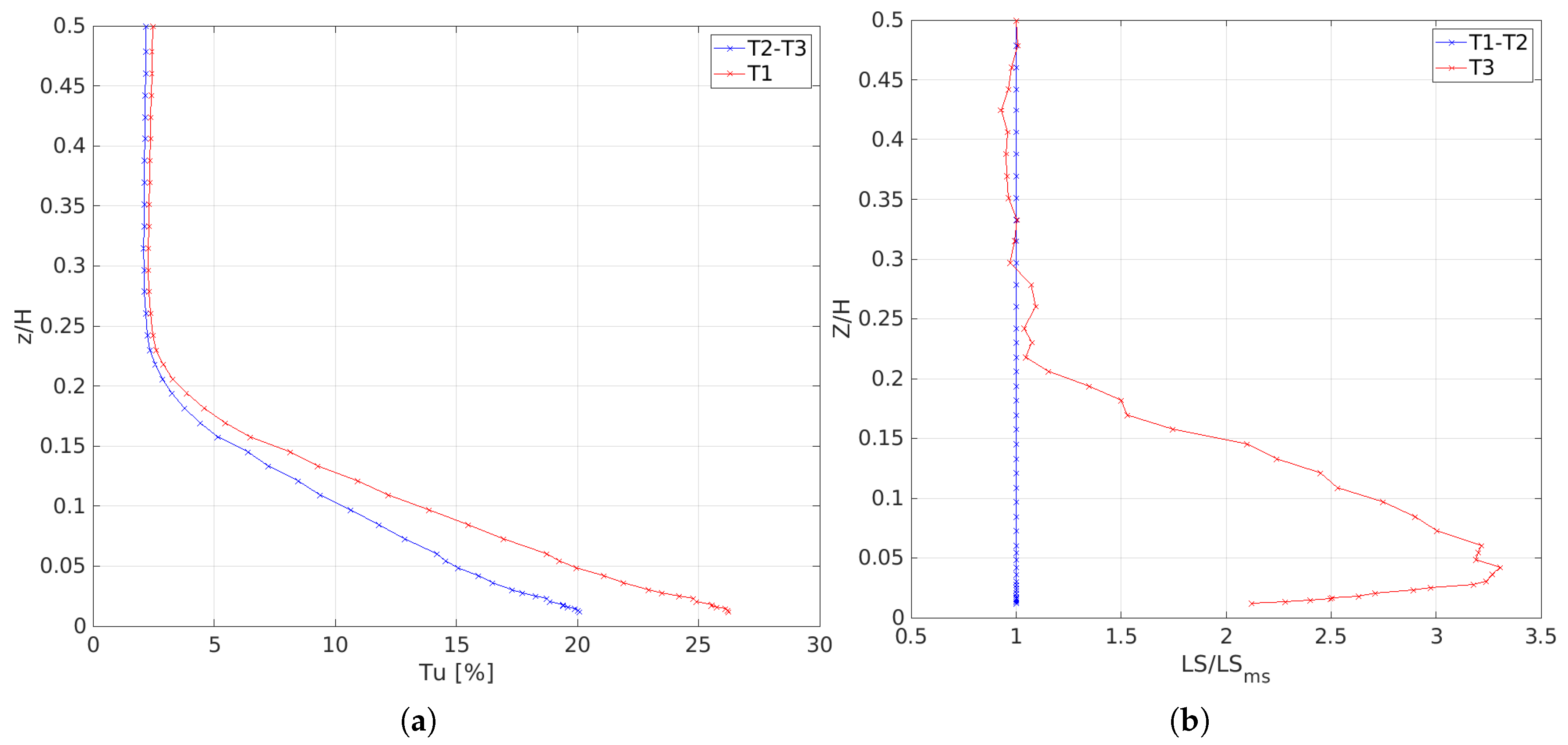
The inlet boundary conditions were prescribed for the present simulations using the experimental spanwise profile for total pressure and incidence angle. Three different turbulence profile specifications were tested, corresponding to the measurements at the inlet plane of the cascade. Turbulence specification is based on the definition of turbulence intensity (Tu) and an integral length scale (ILS).
- T1: The velocity fluctuations at PL02 are post-processed assuming isotropic turbulence, while the turbulent length scale profile is uniform and defined according to the turbulence decay at midspan.
- T2: The velocity fluctuations at PL02 are post-processed assuming anisotropic turbulence while the turbulent length scale profile is uniform and defined according to the turbulence decay at midspan.
- T3: The velocity fluctuations at PL02 are post-processed assuming anisotropic turbulence, while the turbulent length scale profile is obtained by scaling the measured integral length scale profile, matching the decay at midspan.
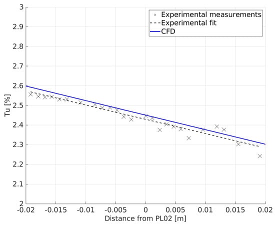
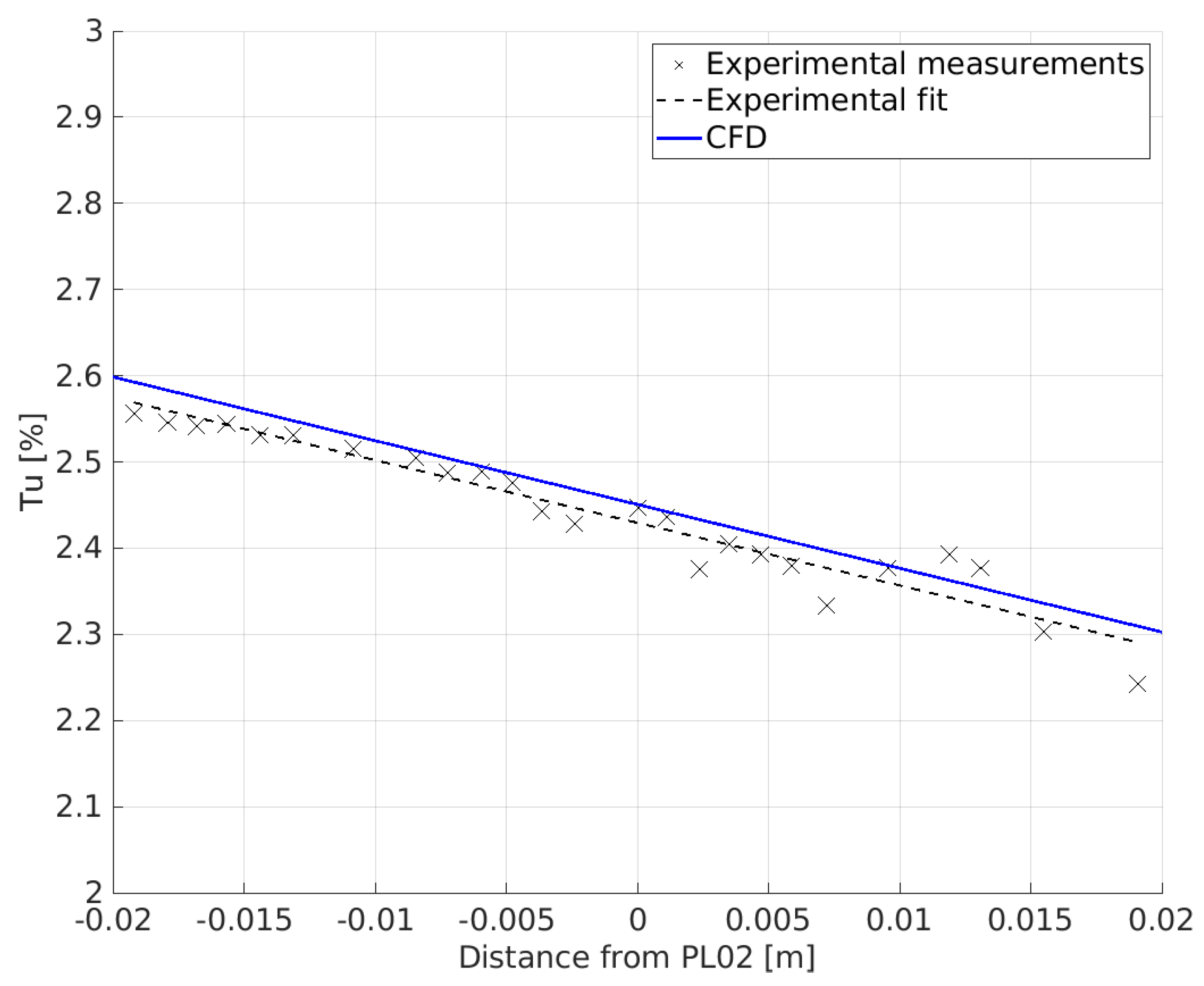
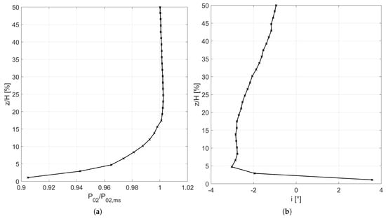
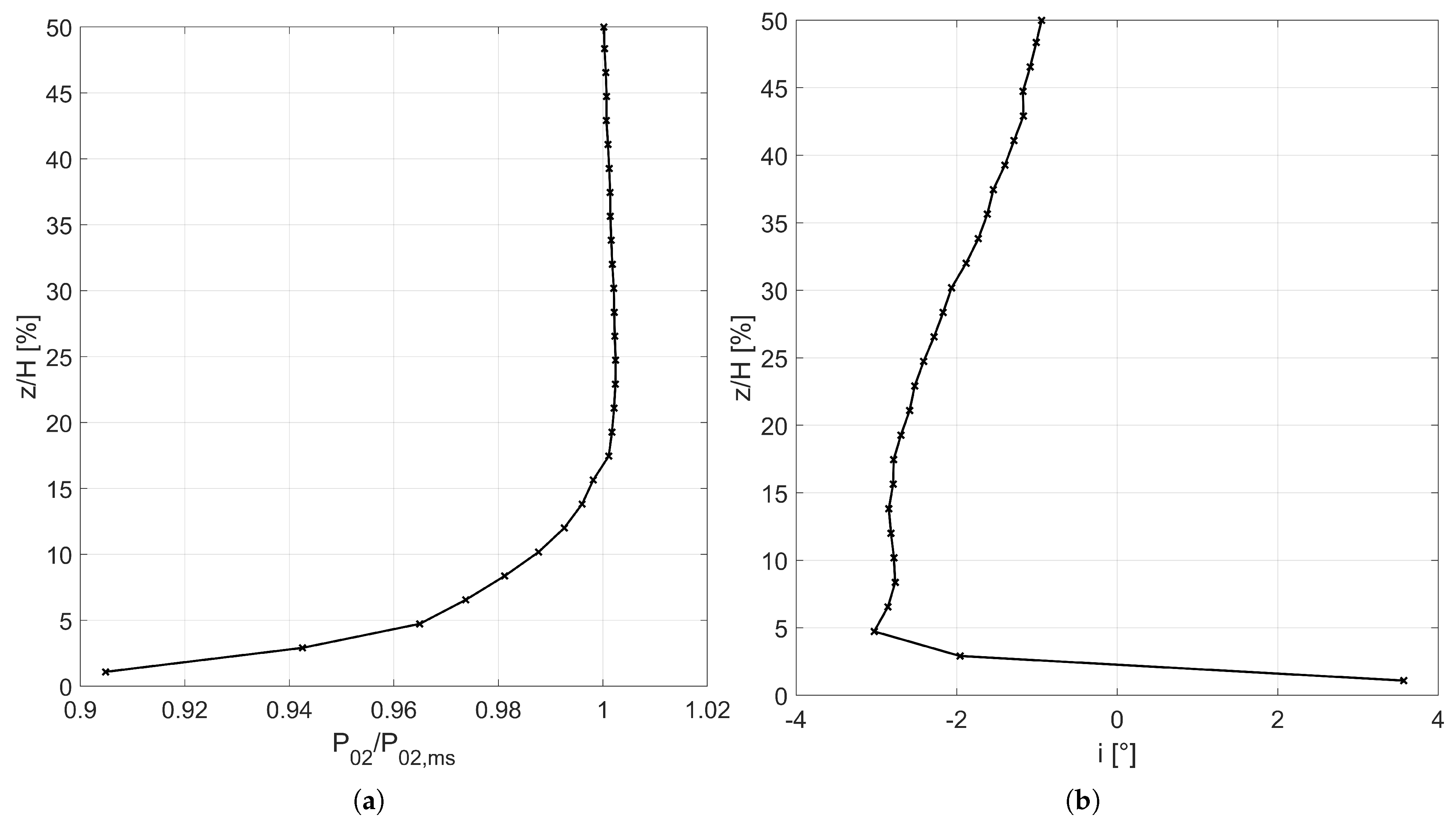
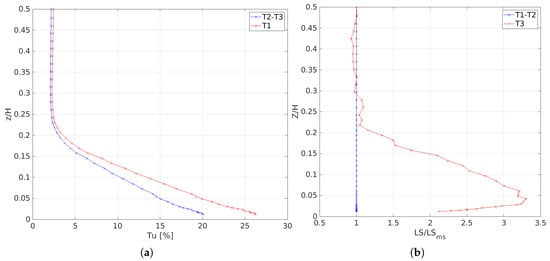
It is important to emphasize that the distinction between isotropic and anisotropic refers to two different definitions used to calculate turbulence intensity. In fact, the first definition considers only the fluctuations related to the axial component, while the second considers an average of the fluctuations of all three components. The matching between the experimental and the numerical turbulence decay at the midspan section of the cascade is shown in Figure 3. The flow’s total pressure and incidence profiles are shown in Figure 4, while mean inlet total temperature is set equal to 300 K. Turbulence profile specification is instead shown in Figure 5. The exact incidence profile was used for both the design and off-design conditions. In contrast, the inlet total pressure profile was scaled (using the inlet Mach number) to guarantee the same velocity profile for all simulations [34]. The equations used to compute the turbulent kinetic energy k and the dissipation are
where denotes the module of velocity while is a non-dimensional constant that depends on the RANS closure model. In the present case, according to [45].
Figure 3.
Midspan turbulence decay.
Figure 4.
Experimental inlet boundary layer profile. (a) Total pressure. (b) Incidence angle.
Figure 5.
Inlet turbulence specification. (a) Turbulence level. (b) Length scale.
4. Grid Dependence
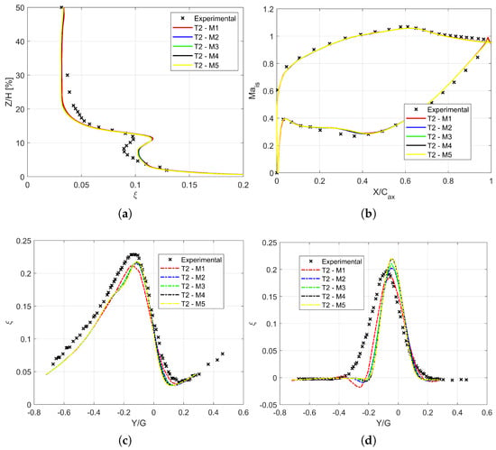
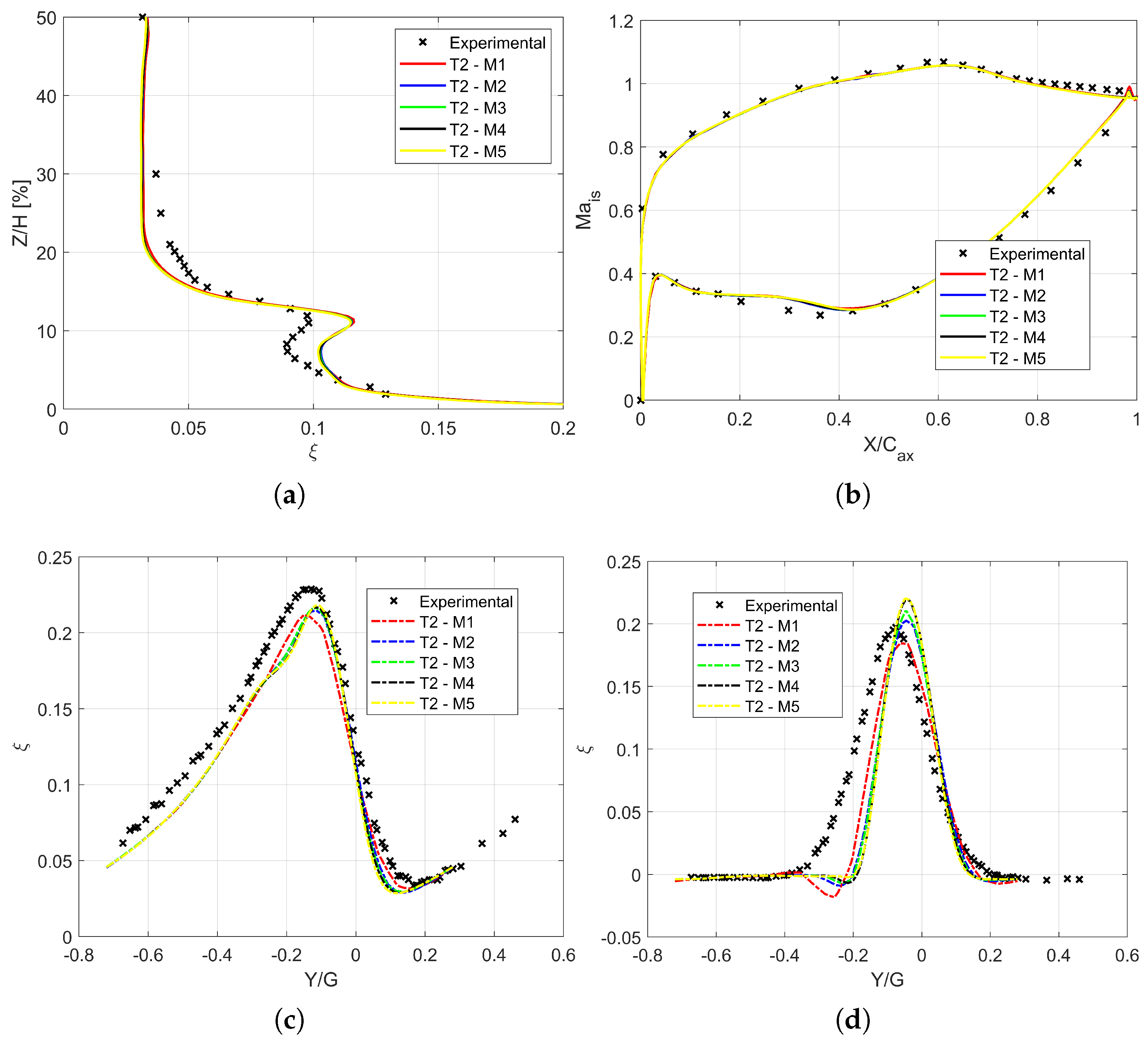
The first part of the numerical activity assessed the solution dependence on the domain discretization. To this purpose, five different meshes were generated through an extrusion of 2D meshes for half of the span of the cascade. All the meshes were generated to obtain a < 1 value over the endwalls and the blade profile. The characteristics of the meshes are listed in Table 4. Grid dependence was assessed regarding blade loading at various span positions, along with overall cascade losses, both pitchwise mass-flow-averaged and pitchwise resolved at different spanwise positions. All simulations were run using the inlet turbulence profile T2. The isentropic Mach number was computed according to Equation (3), while losses are expressed in terms of energy loss coefficient , as defined by Equation (4). Figure 6 reports loading predictions and mass-flow-averaged losses at PL06.
Table 4.
Mesh characteristics.
Figure 6.
Mesh sensitivity results. (a) PL06 pitchwise averaged losses. (b) Blade loading at midspan. (c) PL06 pitchwise resolved losses for Z/H = 5%. (d) PL06 pitchwise resolved losses for Z/H = 30%.
Regarding the loading, all meshes manage to capture the SS evolution of the pressure up to S/S0 = 0.6, while the numerical diffusion is slightly faster than the experimental one. On the other hand, on the pressure side, the loading shows a separation bubble in the region , where the isentropic Mach number features a plateau. While the separation bubble is also present in the experimental measurements, its size is probably smaller than the one predicted by the simulations. In the aft part, the isentropic Mach number is slightly overestimated, which hints at a possible misprediction of the base pressure, together with the faster pressure recovery on the SS. A similar misprediction of the loading has already been reported in [47] for two-dimensional simulations of the midspan flow, and in [48], where the midspan flow section was simulated utilizing a LES approach.
For this reason, the misprediction is not attributed to three-dimensional effects and turbulence specification at the inlet plane. Similar considerations can be drawn from the energy loss coefficient distribution, where the dependency on the grid distribution is not evident. All meshes yield the same profile, recovering the experimental trend regarding peak loss position and shape of the loss coefficient in the endwall region. On the other hand, losses are overestimated for 5% < Z/H < 15%, where the secondary flows accumulate. Another evident misprediction occurs for the mixing region between the hub flow and the central portion of the blade (15% < Z/H < 30%). Experimental measurements indicate a gradual transition from the high-loss to the midspan region, which is not resolved yet at 30% of the span. The numerical counterpart features a fast transition from the loss peak to the midspan loss value, which is recovered for 20% < Z/H. Since averaged values and aerodynamic quantities show a slight dependence on mesh discretization, local flow losses at the outlet measurement plane eventually dictated the final choice. The latter provides a more explicit indication of the dependence of secondary flow development on the mesh size. Figure 6c,d show the pitchwise resolved loss distribution for four different spanwise positions. It is clear that despite all the meshes providing similar results regarding averaged loss distribution, the same does not hold for local flow distribution. Coarser grids generally diffuse the shape while reducing the loss peak. A mesh-independent solution is found only for M4, both for higher spanwise positions and closer to the endwall region. It can also be added that while the agreement at a low span (Z/H = 5%) is good, deviations from measurements arise at higher spanwise positions, where the loss peak is over-predicted, along with the wake position. This agrees with the pitchwise averaged results for the same spanwise locations.
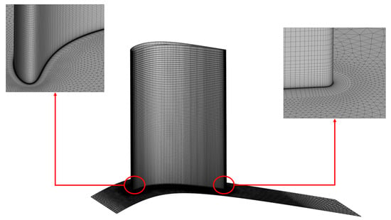
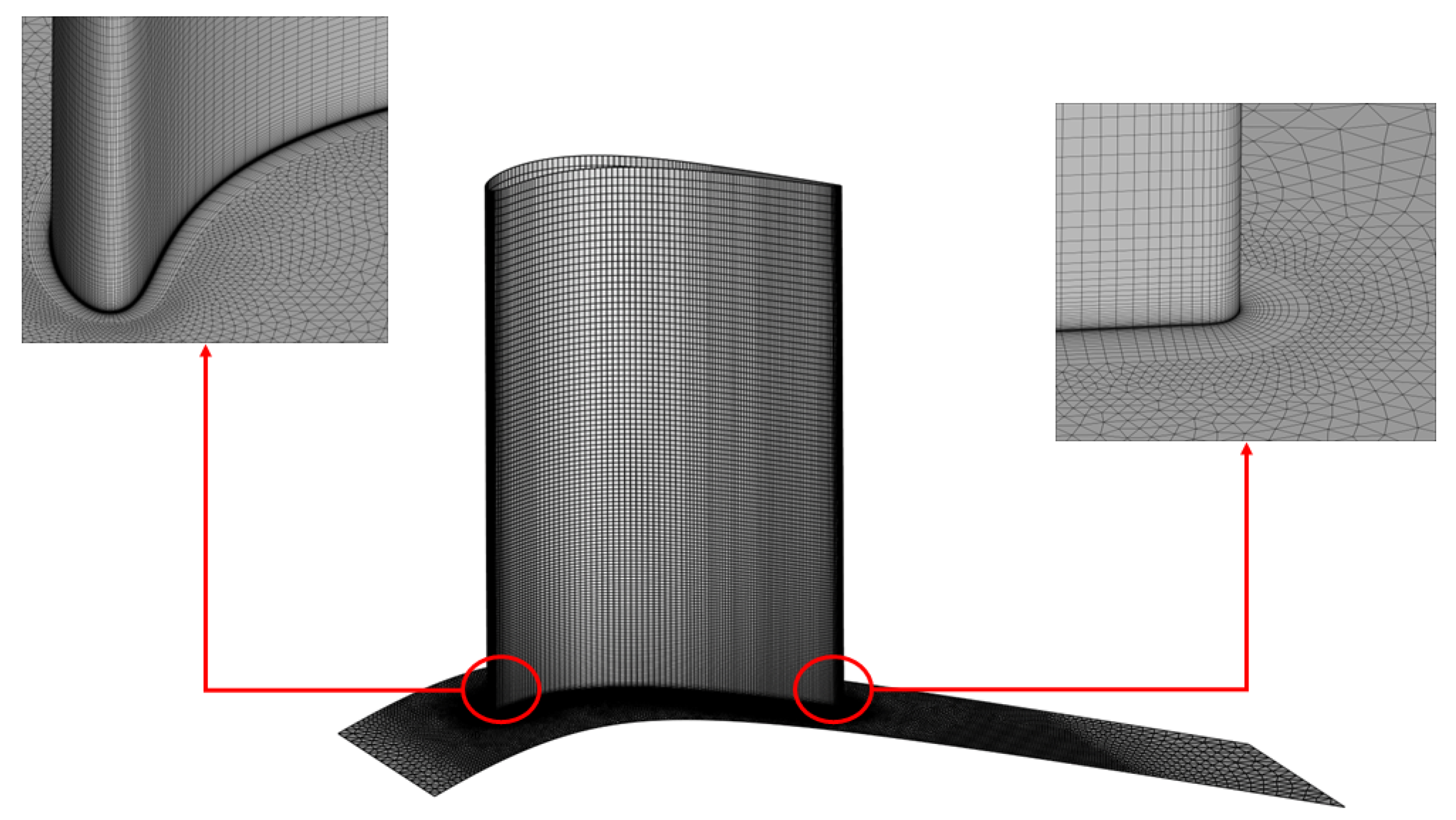
The sensitivity of the secondary loss cores and wake deficit to spatial discretization is consistent with the results reported in [18,21], where it was demonstrated that capturing the exact peak and spread of the losses in the SPLEEN cascade requires very high mesh resolutions and high-order numerical schemes. In this research, mesh M4 was adopted for all the simulations. Close-up views of the LE and TE regions of the mesh are reported in Figure 7.
Figure 7.
Detail of M4 mesh.
5. Results
5.1. Endwall Flow
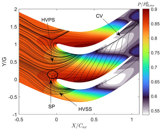
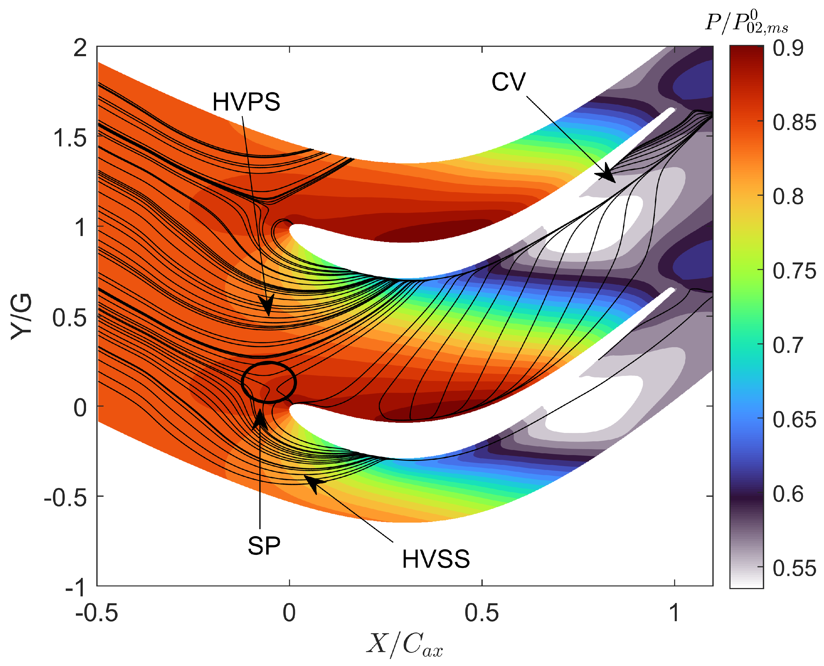
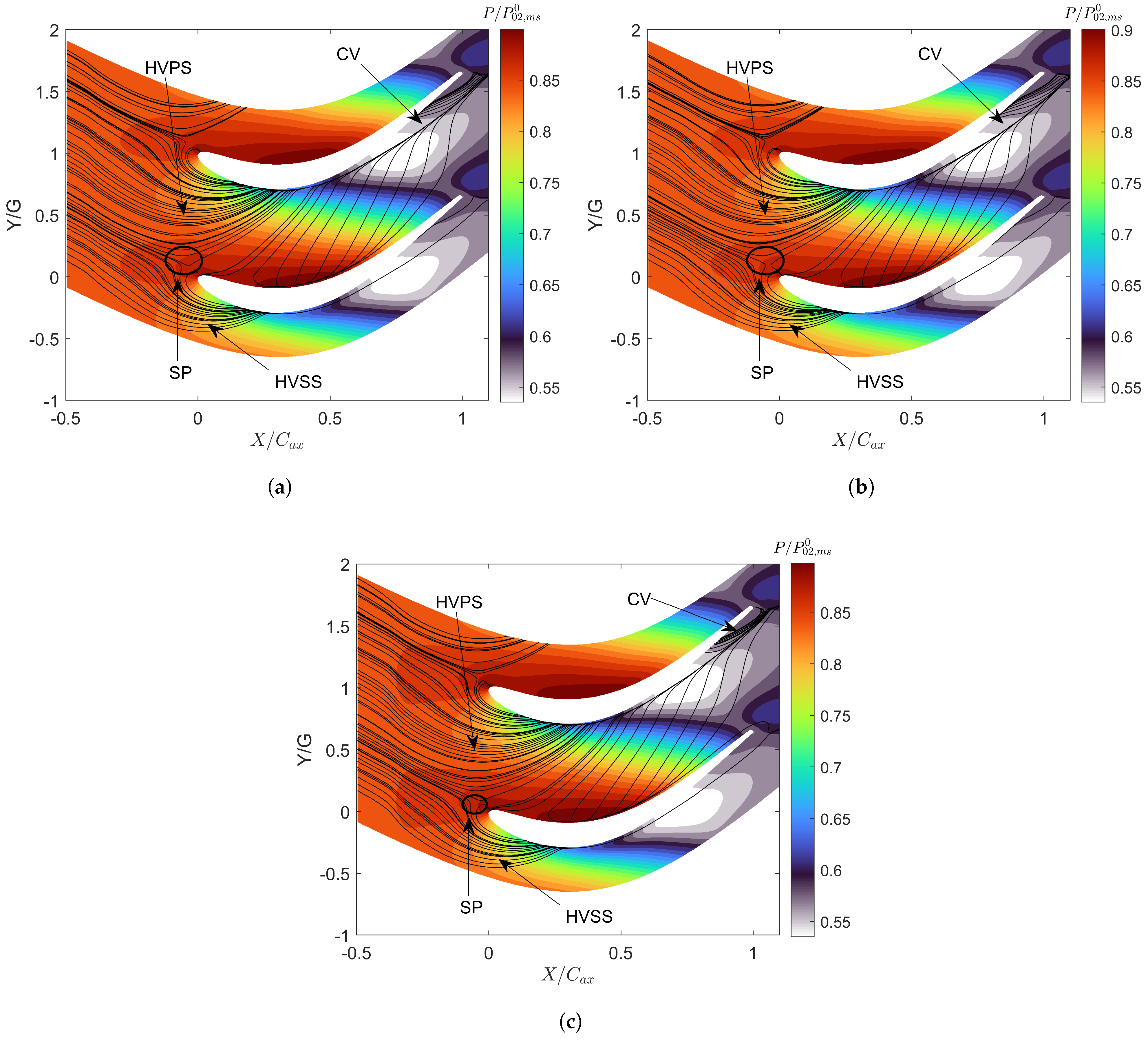
One of the primary sources of losses in the cascade is the development of secondary flows under the incoming boundary layer and the endwall flow. The origin of these secondary flows is first addressed by using visualizations of the streamlines and static pressure over the endwall in Figure 8. The static pressure is normalized by the total pressure of the inlet midspan. The streamlines indicate the origin of the horseshoe vortex upstream of the blade LE and the bifurcation of the endwall flow into a PS leg, which travels towards the blade SS, and an SS leg. The endwall limiting lines feature a single saddle point upstream of the LE. The SS leg interacts with the PS leg, which is transported towards the blade suction side. After the impingement of the HV structure on the blade SS, a corner vortex (CV) originates in the aft region of the blade, providing local blockage to the flow.
Figure 8.
Endwall streamlines.
5.2. Transport of Secondary Flows
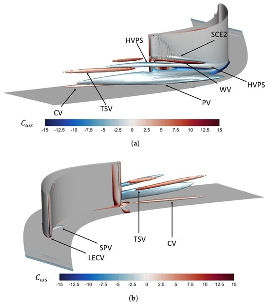
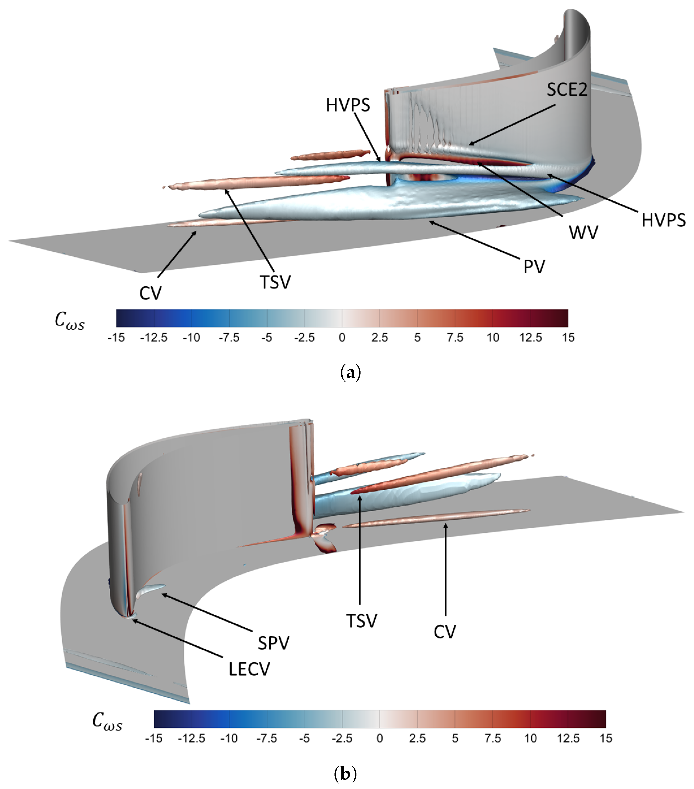
A general overview of the vortical structures is displayed in Figure 9, which shows Q-criterion iso-surfaces at , obtained using the T2 turbulence profile. The plots are cut at 30% of the spanwise coordinate to highlight the region affected by the development of secondary flows. Iso-surfaces are colored with streamwise vorticity coefficient (Equation (5)). The streamwise vorticity is defined according to Equation (6), where is the midspan flow angle, while and are the axial and pitchwise vorticity, respectively.
Figure 9.
Q-criterion vortex. (a) Suction side. (b) Pressure side.
The Q-criterion shows five structures that develop throughout and downstream of the cascade. The PS leg of the HV stems from the inlet boundary layer separation upstream of the blade’s leading edge and lifts upon reaching the blade SS. Its interaction with the endwall boundary layer and suction-side boundary layer generates secondary vortical structures. The latter is counter-rotating with respect to the HVPS and will be referred to as the wall vortex (WV) throughout this paper. A secondary vortex, co-rotating with the HVPS, develops over the endwall, induced by the pressure gradient between the PS and SS, and is referred to as the passage vortex (PV). The structure attached to the cascade hub is the corner vortex (CV), counter-rotating with respect to the HVPS. A fifth vortex structure arises downstream of the cascade, referred to as a trailing shed vortex (TSV), induced by a total pressure deficit in the inlet boundary layer.
Other minor vorticity regions can be appreciated as well. The leading edge corner vortex (LECV) develops at the junction between the endwall and the blade LE. In addition, the spanwise migration of both the WV and HVPS on the SS also induces another vorticity region, which will be referred to as the suction corner endwall separation (SCE2), after [49]. The latter is co-rotating with the HVPS. The last vorticity region is called the separation vortex (SPV) and originates from flow separation over the pressure side of the blade. A similar structure is reported in [50].
5.3. Blade Predictions
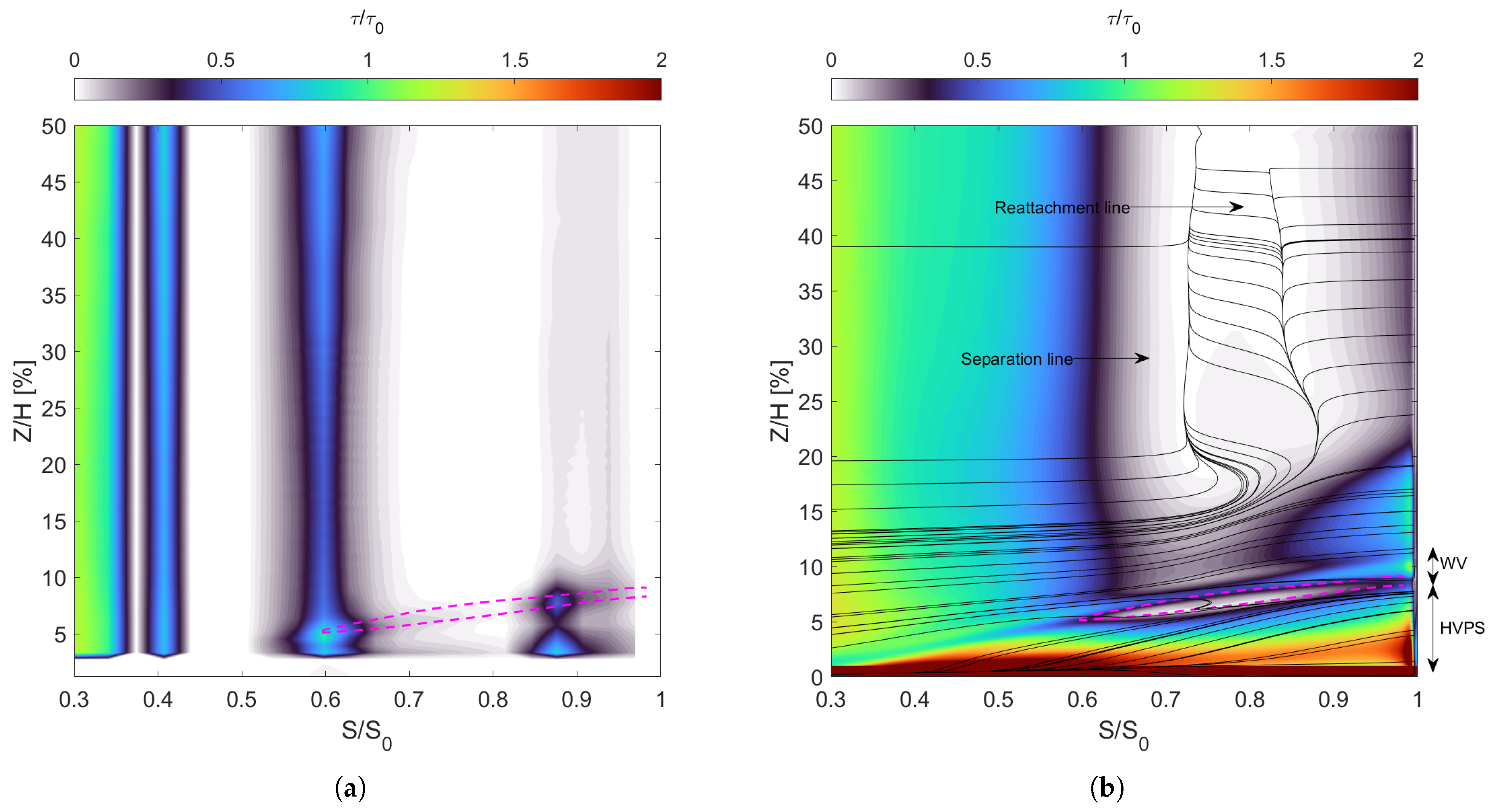
The spanwise development of the secondary flows and the separation upstream of the leading edge affect the blade flow. Figure 10 shows the experimental and numerical normalized wall shear stress. Normalization is performed using, for each dataset, the corresponding wall shear stress at 20% of the curvilinear coordinate in the LE region (), thus highlighting relevant flow structures for a quantitative comparison. Streamlines are super-imposed to the contours of the numerical predictions to show the development of the secondary vortices, along with the boundary layer separation at higher midspan positions (Z/H < ). The SS flow is characterized by the vortices developing throughout the cascade: CV, HVPS, and WV. The position of these vortices can be identified in the numerical predictions: the CV close to the endwall and the HVPS vortex below the WV vortex. The regions of low wall shear stress between the vortices are due to vortex cancellation, which leads to a change in the sign of the spanwise shear stress. The dashed lines (in magenta color) allow tracking of the HVPS and WV positions along the suction side. The lower one corresponds to a minimum wall shear stress corresponding to WV/HVPS vortex cancellation. The upper one tracks down a local peak induced by the passage of the WV.
Figure 10.
Blade wall shear stress. (a) Experimental data. (b) CFD.
Numerical simulations also clearly show the separation line, which stems from 20% of the span up to the midspan of the cascade and the consequent reattachment line of the separation bubble. In the experimental measurements, the CV cannot be retrieved due to the position of the hot films. Despite this, according to [15], the trajectory of the wall-induced vortex and the passage vortex can be retrieved from the regions of high wall shear stress values. A comparison with the numerical results (whose lines are shown on the plot) indicates that CFD tends to predict a slightly higher position of the vortical structures than the measurements. Out of the endwall flow region, the decrease in the wall shear stress after the velocity peak is faster in the experiments compared to numerical predictions (S/S0 < 0.5). For S/S0 < 0.6, low shear stress values are found. This is caused by a separated or near-separated boundary layer, which agrees with the numerical predictions of a separated boundary layer.
The over-prediction of the pressure-side separation bubble and the discrepancies in the suction-side pressure recovery observed in the present results are well-documented challenges for this cascade. Recent high-fidelity Wall-Resolved LES studies and multi-fidelity RANS assessments [20,22,23,39] have reported similar struggles in capturing the transition onset and the open separation bubble without resolving the smallest turbulent scales. Detailed validation of these phenomena, particularly regarding turbulence anisotropy and secondary flow boundaries, is supported by recent experimental campaigns through Particle Image Velocimetry (PIV) [51].
5.4. Effect of the Inlet Turbulence Profile
In this section, the effect of the inlet turbulence profile will be analyzed in terms of endwall flow distribution, outlet losses, and loading predictions close to the cascade hub. The three turbulence profiles used in the calculations (Figure 5) are different in terms of Tu distributions and peak and LS, affecting the decay of turbulence intensity upstream of the LE. The simulations were run using the same total pressure and incidence angle profiles.
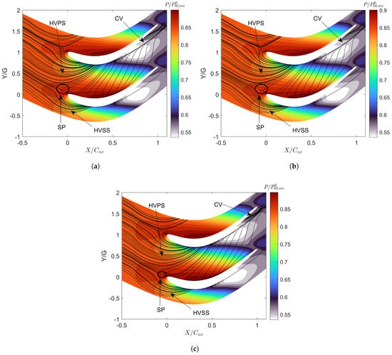
Figure 11 shows the effect of the turbulence profile on endwall flow distribution, particularly on the generation of the vortex system of the cascade. Profiles T1 and T2 present the same uniform ILS profile (see Figure 5b), but the former features higher turbulence levels in the inlet boundary layer. The streamline system predicted with these two conditions is similar, clearly highlighting the behavior of the HV legs and the CV. The saddle point is in the same location, while the CV structure holds the same extension. The T3 case, instead, marks the effect of the LS profile over the predictions of the endwall flow. Also, the overall distribution of the secondary flows is similar, but two slight differences compared to the profiles T1 and T2 occur. The saddle point moves slightly downstream because of the slower decay achieved by employing a higher turbulent length scale at the profile inlet. On the other hand, the CV seems weaker, based on the streamlines close to , which retains an effect on the blade pressure distribution in the hub region.
Figure 11.
Endwall streamlines: Effect of turbulence profile. (a) T1. (b) T2. (c) T3. Positions of the saddle point in (, ): (a) (−0.082, 0.125); (b) (−0.080, 0.123); (c) (−0.075, 0.118).
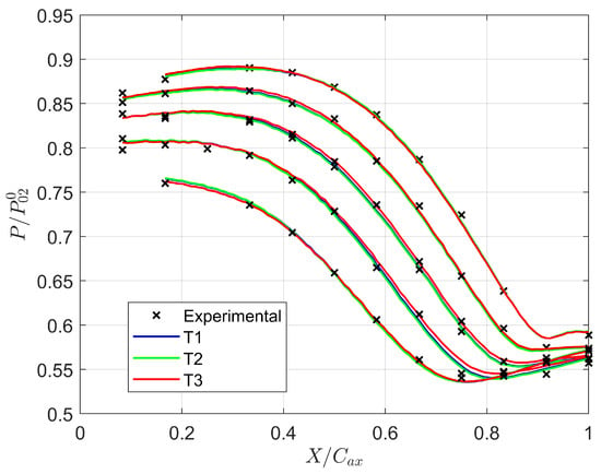
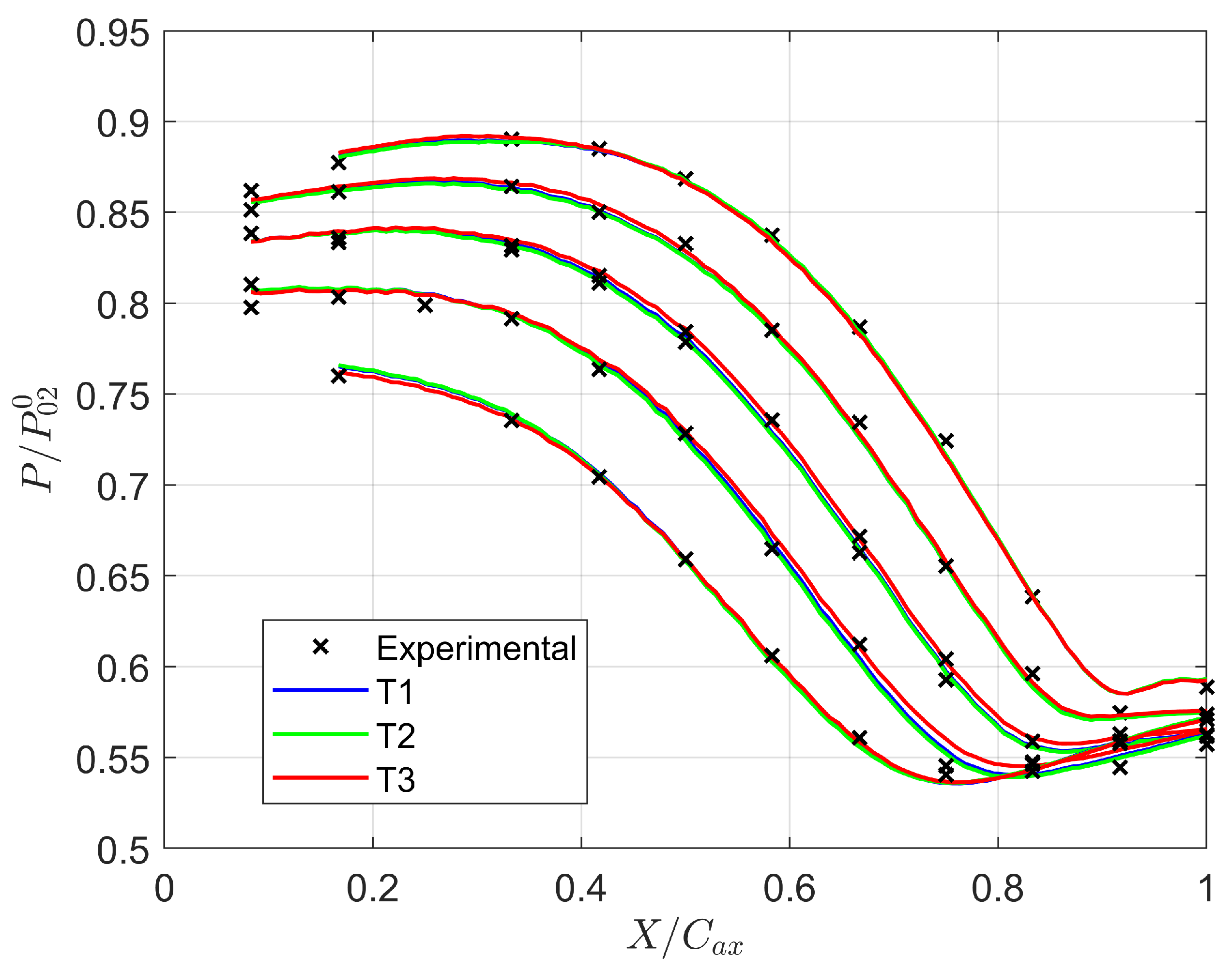
The numerical predictions of the static pressure over the endwall and the experimental measurements are compared in Figure 12. The experimental points refer to the measurements obtained for two different blade passages, so the results at some axial locations are duplicated. The slight difference over the endwall streamlines also reflects on the pressure distribution.
Figure 12.
Effect of turbulence profile: Endwall static pressure.
The CFD results match the experiments very well, regardless of the prescribed inlet turbulence profiles. While profiles T1 and T2 feature the same pressure distribution, some differences arise for profile T3. The effect of the slower turbulence decay of the profile is visible at the LE of the blade. T3 yields a higher loading in the front part of the blade induced by the increased acceleration over the SS. The situation is opposite at the TE, where the T3 features a lower loading than profiles T1 and T2. This is instead adduced to the different sizes in the predicted corner vortex.
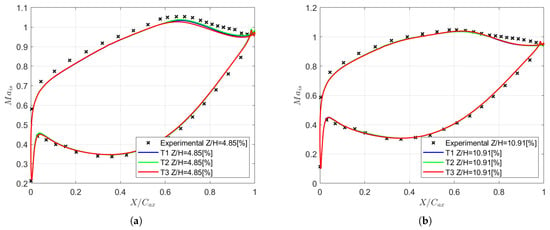
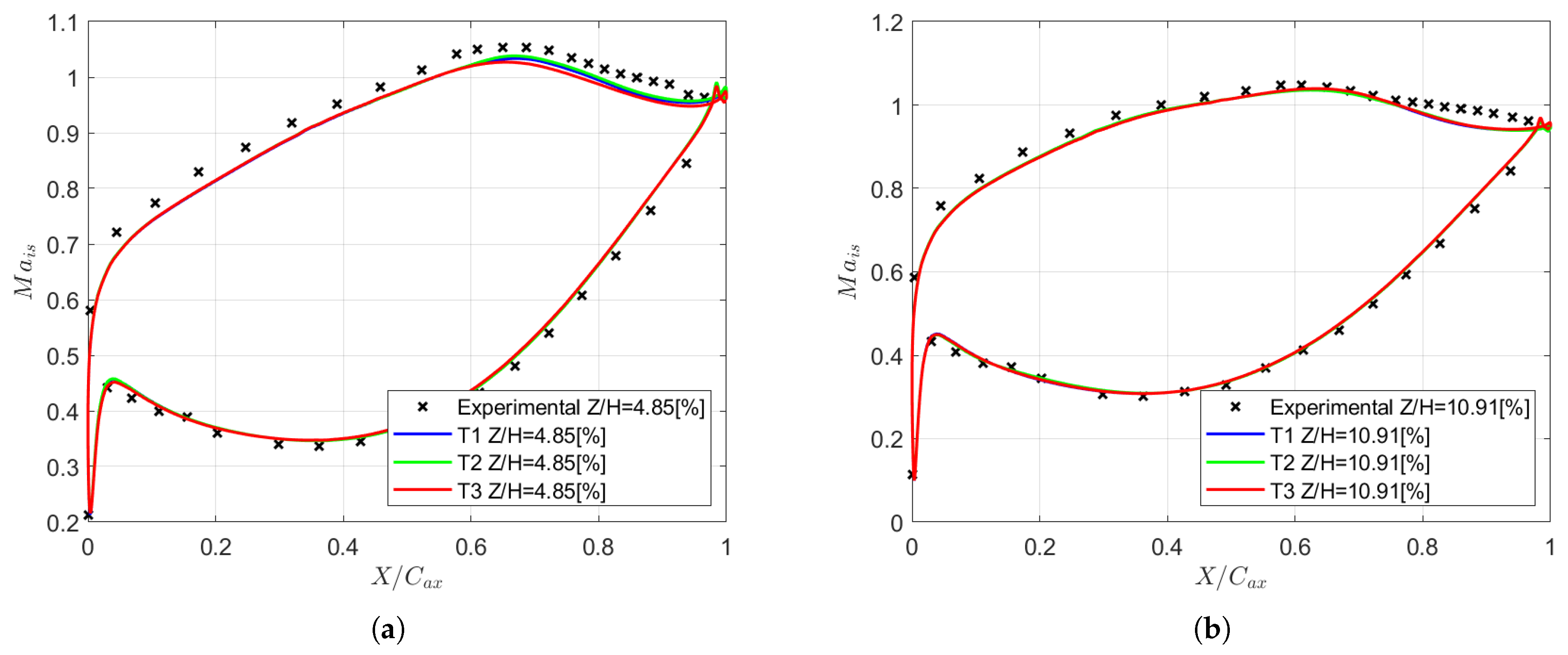
Figure 13 shows the predictions of blade loading at various span positions compared with experimental measurements. The discussion will start with profiles T1 and T2. In the endwall region at Z/H = 4.85% (Figure 13a), CFD matches the loading distribution close to the LE, both on the pressure side and the suction side, but underestimates the acceleration on the SS. The PS is correctly retrieved up to = 0.6, while an overestimation of the isentropic Mach is found downstream, up to the TE.
Figure 13.
Blade loading. (a) %; (b) %.
Similarly to the previous case, the isentropic flow velocity is underestimated on the SS, even if the experimental shape is correctly retrieved. The peak velocity is predicted to be at 0.65, in a similar location compared to the experiments. Experiments also evidence the initiation of a thick boundary layer over the last region of the SS, which is evident from the third-last measurement point at = 0.85. At Z/H = 10.91%, the agreement between the CFD and the experiments is better in the accelerating region. Despite this, simulations do not succeed in predicting the pressure recovery in the aft portion of the SS. Simulations predict fast pressure recovery, contrary to the experiments. The results at Z/H > 20.61% are comparable to what is found at the midspan, both in the CFD and in the experiments, and the same misprediction of the PS separation bubble and the SS pressure recovery introduced in Section 4 is present in the aft region. Hence, they are omitted for brevity.
Very tiny differences are instead induced by the variation in the inlet turbulence specification, which is concentrated in the hub region (Figure 13b). The peak velocity increases for higher turbulence level specifications (T1) and slower turbulence decay (T3) compared to our baseline configuration (T2). At Z/H = 1.21%, the effect is more evident and is supported by the lower size of the CV. For higher spanwise positions, the inlet turbulence specification does not affect the predicted loading, indicating a low sensitivity of the setup on the definition of both the turbulence intensity and the length scale.
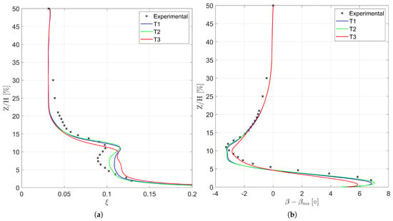
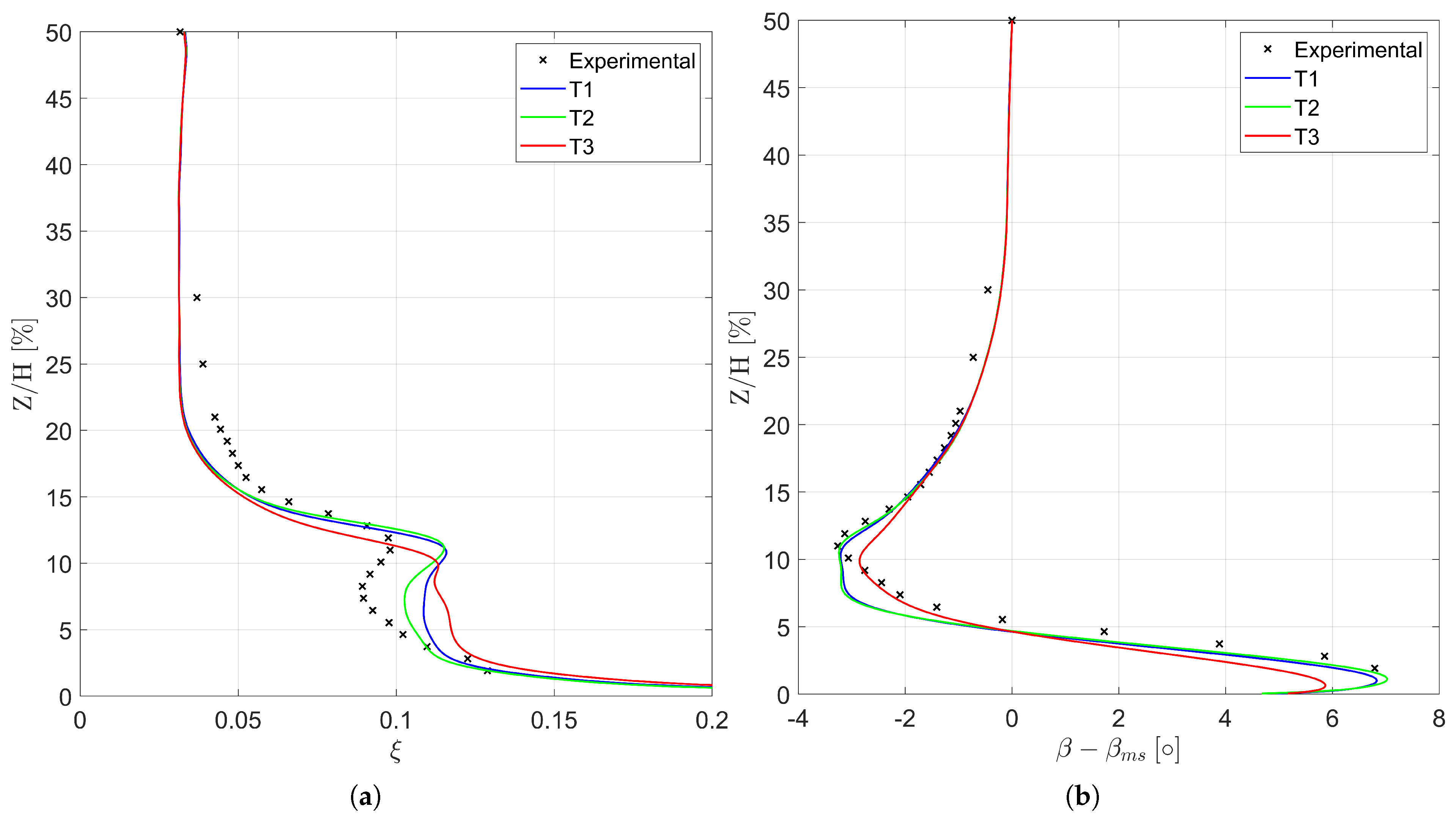
The spanwise distributions of mass-flow-averaged losses are shown in Figure 14a. Profile T1 has a good prediction of the experimental measurements up to 5% of the span. Above that, losses show a flat loss profile, which does not agree with the experimental predictions. Profile T1 has a systematic over-prediction of the losses in this region compared to experimental values, showing a peak at Z/H = 11.5%. The position is under-predicted compared to the experiments. Better agreement between the experiments and CFD is found for profile T2, as shown in Section 4. In this case, the trend in the losses is correctly predicted up to 5% of the span.
Figure 14.
Effect of turbulence profile on the outlet flow field. (a) Spanwise distributions of pitchwise mass-flow-averaged losses. (b) Spanwise distributions of pitchwise mass-flow-averaged deviation angle (referred to as the midspan value).
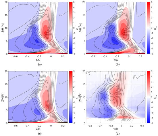
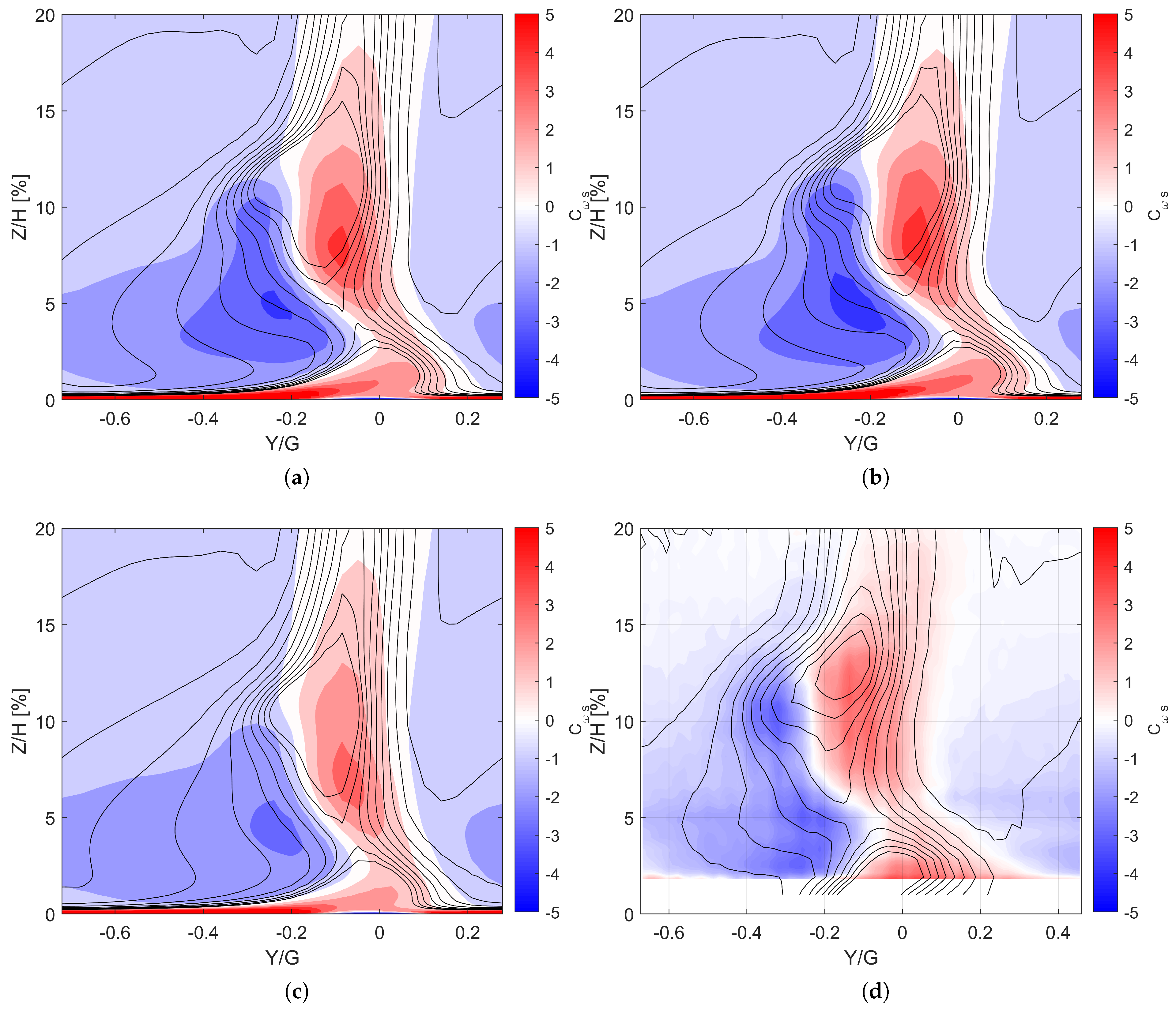
Similarly to profile T1, T2 has an over-prediction of the peak of the losses. Numerical predictions show a peak of approximately 0.12, while the corresponding experimental value is ≈0.10. The spanwise position of the peak of the losses is well predicted with both inlet turbulence profiles (Z/H = 11.5% for T1, Z/H = 11.9% for T2, and Z/H = 11.9% for the measurements). The main difference between the two profiles occurs between the peak and the endwall. Despite the over-prediction, the T2 profiles show reduced losses, with a local minimum at Z/H≈ 7.5%, as found in the experiments. Concerning profile T3, the loss distribution is much smoother, with no evident peak along the spanwise coordinate. This results from the weaker vortical system generated with this turbulence profile, as visible in Figure 15. Losses are systematically over-predicted in the endwall region, while an underestimation of corresponds with the experimental peak. The correct prediction of the losses is only found at the midspan. The trend in the losses can be easily explained considering the spanwise migration of the vortical system arising from the transport of the inlet and endwall boundary layer. Profiles T1 and T2 feature an important migration of the secondary flow features throughout the cascade, transporting low-momentum flow from inlet and endwall boundary layers towards the span of the blade. On the other hand, when the strength of the vortices is lower, the lift effect is weak and low-momentum flow remains close to the endwall region, where the low total pressure induces high values of .
Figure 15.
Outlet measurement plane. (a) T1. (b) T2. (c) T3. (d) experimental.
Figure 14b shows the measured and predicted pitchwise mass-flow-averaged deviation angle referred to as the midspan value. Similarly to the losses, profiles T1 and T2 feature the same predictions of flow angle, both close to the endwall and in correspondence with the under-turning found in the correspondence of the loss peak. In the 5% < Z/H < 12% region, the flow angle distribution is much smoother compared to the experimental one. This characteristic can be attributed to the insufficient mixing of the secondary flows and the generally over-predicted system strength, as shown in Figure 15. Turbulence profile T3 instead features a smoother spanwise variation in the deviation angle for Z/H < 9%. Despite a better agreement with the shape’s experimental averaged deviation, the profile yields misprediction both over the endwall and in the loss peak region. The over-turning over the hub is overestimated by roughly , while the under-turning at Z/H = 11.5% is underestimated by ∼.
The flow field at the outlet measurement plane (PL06) is shown in Figure 15, along with isolines of the total pressure loss coefficient. This figure also shows the experimental measurements of streamwise vorticity and the loss coefficient for the same plane. Profiles T1 and T2 feature similar distributions both for losses and vorticity. The main difference is present in the PV structure, which is more relevant for profile T2 reaching a peak value of −3.36 with respect to the corresponding value of obtained for the T1 profile and the found for the T3 profile. Concerning the latter case, it is also possible to conclude that the vorticity is greatly dissipated, thanks to the lower turbulence intensity imposed on the inlet plane. Both T1 and T2 profiles match the experimental distribution of the vorticity even though the experimental flow structures appear mixed-out with respect to the numerical ones due to the limitations associated with RANS approaches. Despite this, it is possible to discern the PV and the HVPS as negative vorticity regions, along with the merged WV+TSV structure in the positive vorticity region. The positioning of experimental sensors instead cuts out the CV. Profile T3 features lower residual vorticity levels in the outlet plane, and only two main rotating cores are found since the HVPS is strongly dissipated. They correspond to the PV and the WV+TSV structure.
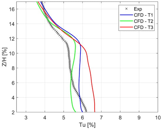
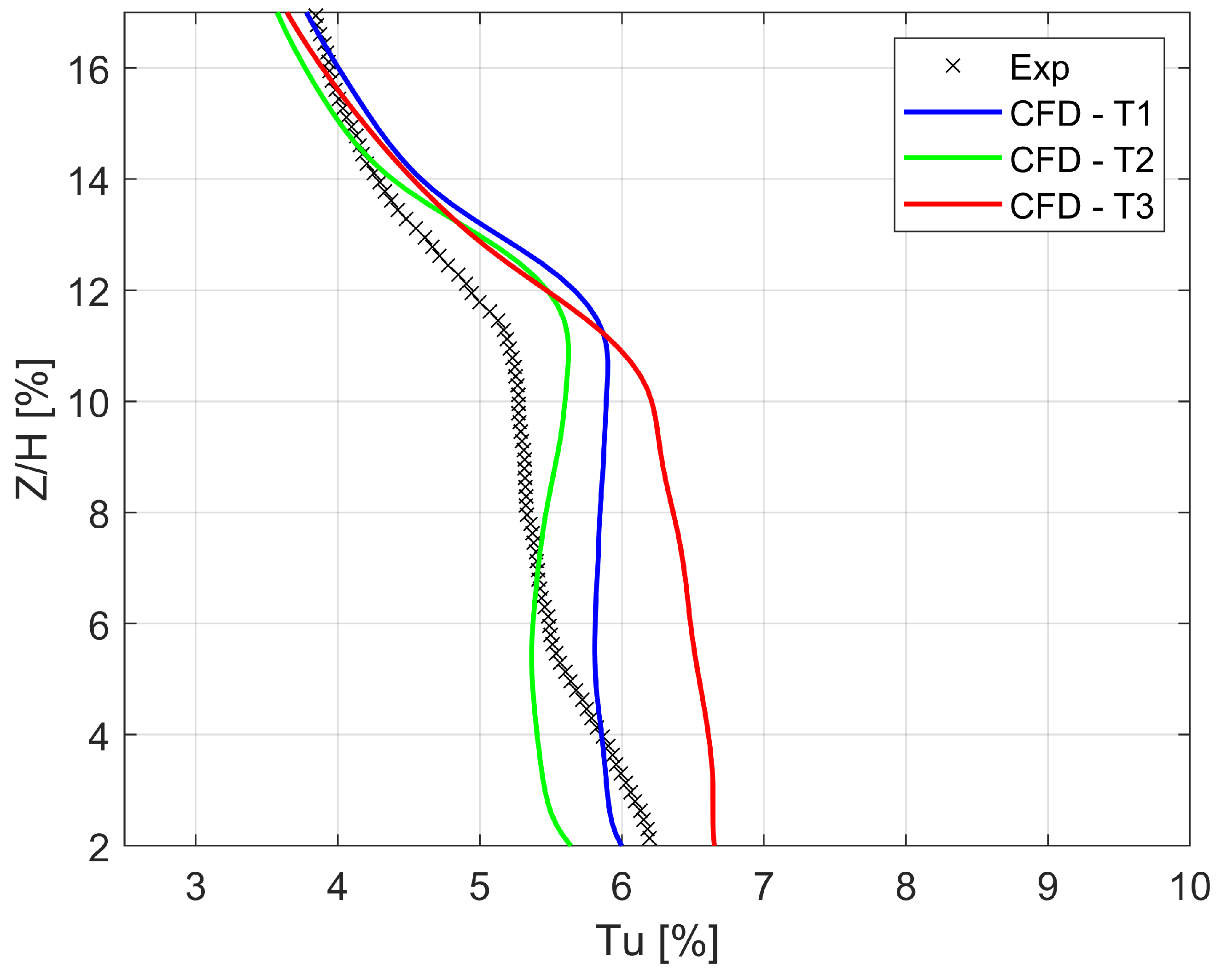
The average turbulence intensity predicted at PL06 is compared with the experimental PIV measurements in Figure 16. The experiments show an increase in Tu towards the endwall, with a concentration at around 11.5% of the spanwise coordinate. T1 and T2 reveal a similar prediction up to the loss peak (Z/H between 16% and 12.0%), with a maximum value of 5.5% and 5.85%, respectively. The lower intensity observed with respect to profile T3 below Z/H = 11% is induced by the lower value of the inlet dissipation rate, which propagates throughout the cascade.
Figure 16.
PL06: Average turbulence intensity.
5.5. Off-Design Conditions
The effect of off-design conditions on the cascade performance was studied, varying independently of the isentropic-outlet Reynolds and Mach numbers. All the off-design conditions were run using the turbulence profile T2, which guaranteed a better prediction of the pitchwise mass-flow-averaged losses at the outlet measurement plane, at least for nominal conditions.
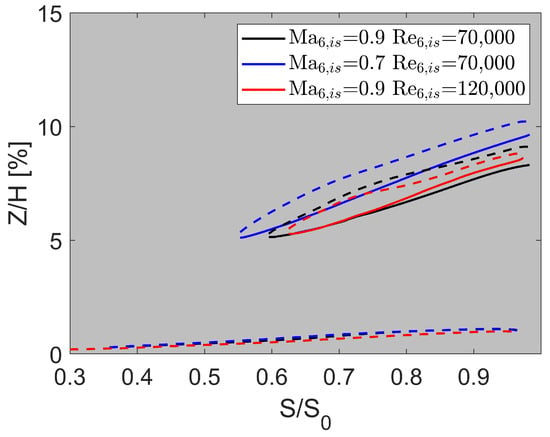
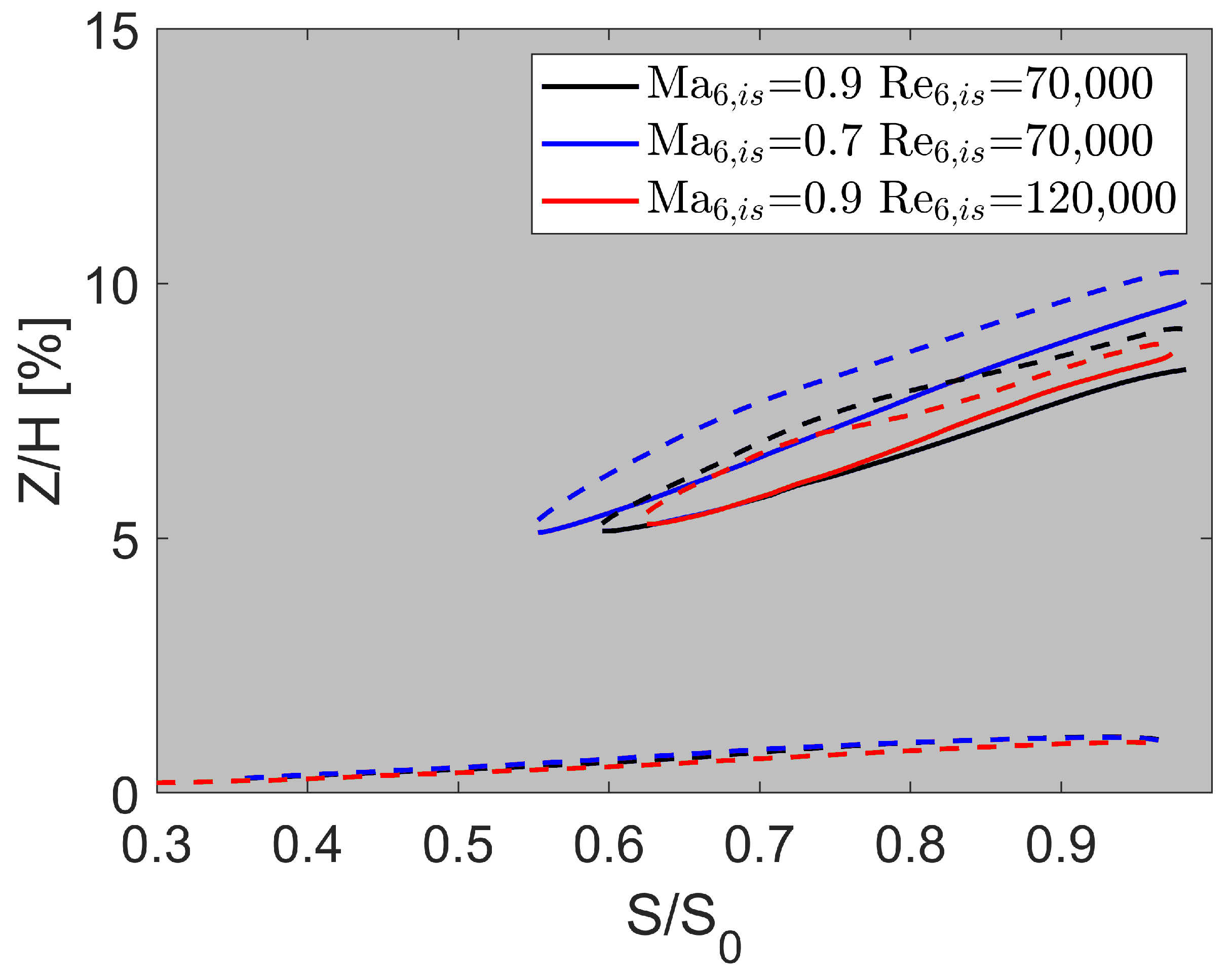
The effect of the operating conditions on the development of vortex structures will be analyzed. Figure 17 shows the extension of the corner vortex, the line separating the PS leg of the horseshoe vortex and wall vortex, and the wall vortex trajectory for the tested operating conditions. While the development of the corner vortex is hardly affected by the working conditions, the same does not hold for the HVPS and the WV. It is shown that a decrease in the isentropic Mach number leads to a stronger development of the vortices in the spanwise direction, induced by the lower axial velocity of this condition. At = 120,000 instead, the position of the WV is found at a lower spanwise position, while vortex cancellation occurs over a similar line compared to the nominal conditions.
Figure 17.
Vortex development: Effect of operating conditions.
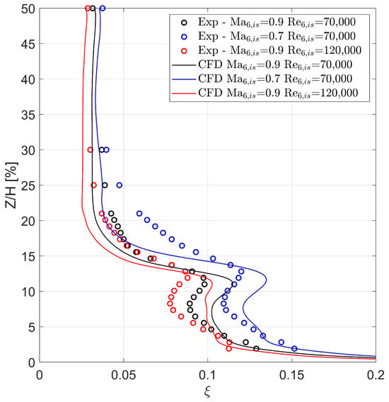
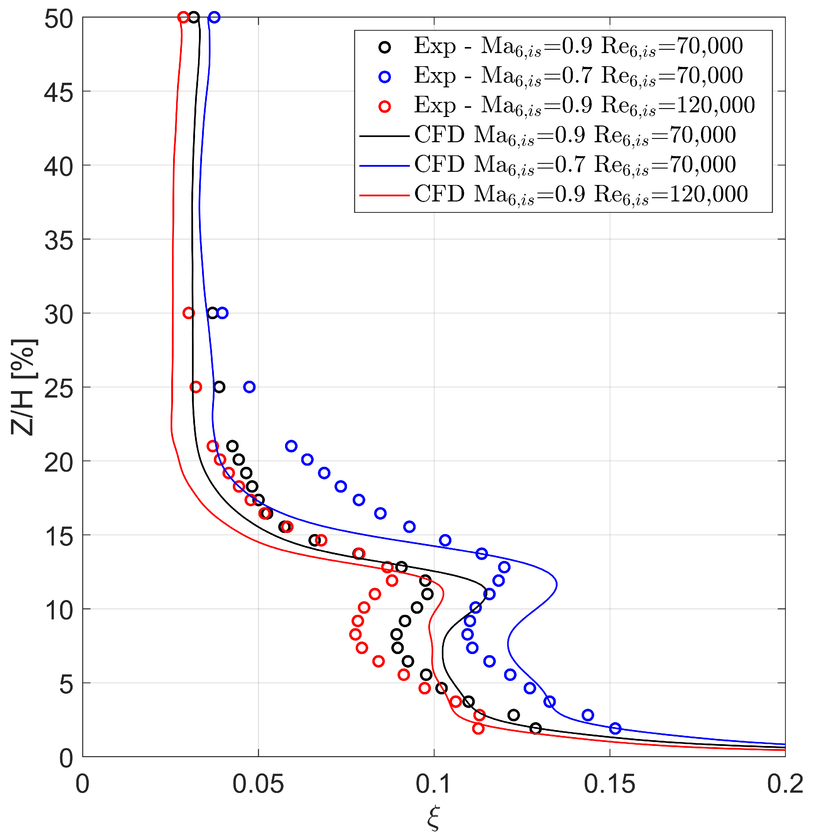
This is coherent with the mass-flow-averaged outlet losses shown in Figure 18. The overall agreement between the CFD predictions and the experimental measurements at nominal Reynolds is good in the endwall region. At the same time, low-Mach conditions show the same behavior as nominal Mach. The losses in the secondary flow region are overestimated: the experimental peak is approximately 0.12, while the numerical peak is 0.13. On the other hand, the trend is captured correctly at = 70,000, as both nominal Mach conditions and low-Mach conditions predict a recessing loss profile below the peak. A lower Mach number induces a higher position of the secondary flow region, with an overall increase in the losses over the whole span of the blade. Similar mispredictions occur above the loss peak (Z/H > 13.5%), where the transition from the high-loss region to the midspan flow for the CFD occurs over a small spanwise extent of approximately 7.5% of the blade span. The lowest losses occur at = 120,000 in the experiments and the CFD. In this case, the numerical setup does not correctly capture the overall loss level or the experimental shape distribution. At lower Reynolds, the loss profile in the endwall region is very smooth, which does not agree with the experimental counterpart and the results at nominal Reynolds. To the authors’ knowledge, this behavior is attributed to the specified inlet turbulence profile. It must be remembered that the latter was measured for the design point ( = 0.9, = 70,000), while no detailed knowledge is available for the high-Reynolds conditions. The second significant difference between the numerical predictions and experimental findings resides in the core spanwise position. CFD tends to predict a lower spanwise position for the loss core at high Reynolds, while experiments show the opposite, the loss core moving from Z/H = 11% to Z/H ≈ 12%.
Figure 18.
Outlet losses.
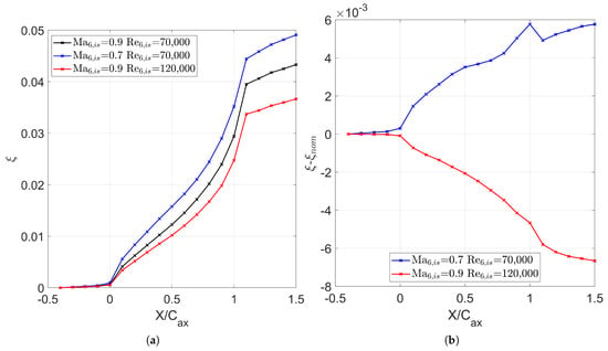
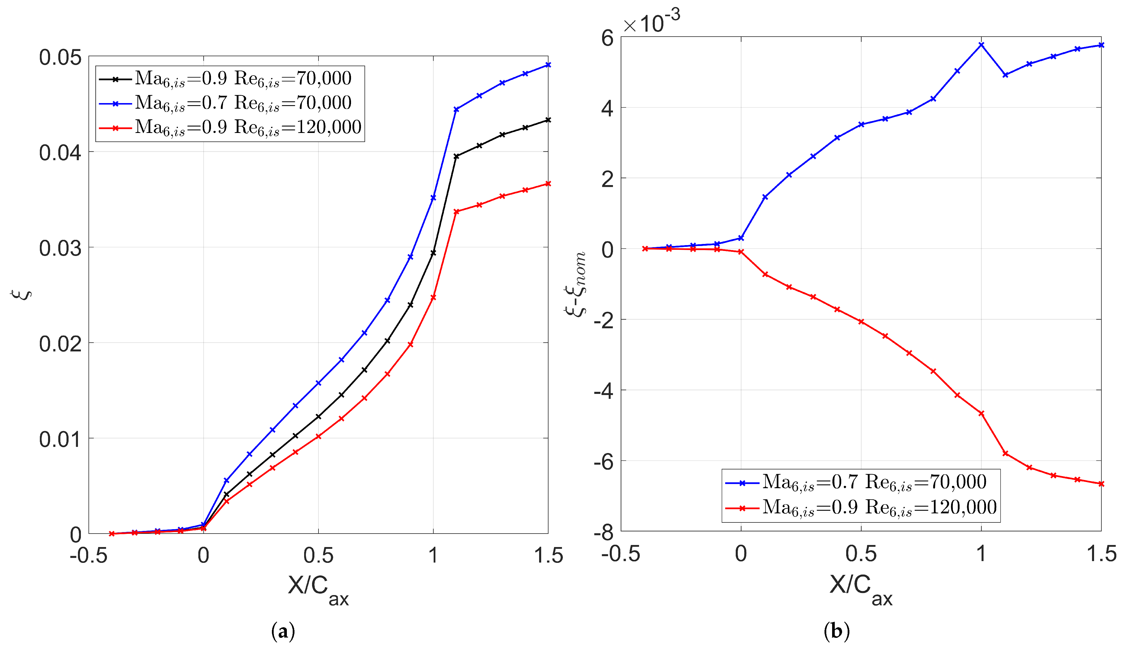
To compare the origin of the losses, the axial development of the loss coefficient is shown in Figure 19. Figure 19a shows the development for the various conditions, while Figure 19b reports the difference for each tested condition with respect to the nominal case ( = 0.9; = 70,000). The region upstream of the LE accounts for upstream endwall losses related to the viscous forces in the endwall boundary layer and the start of the roll-up of the HV vortex. In the region in the range of 0 ≤ ≤ 1, the increase in the losses is related to the development of the profile and endwall boundary layer, plus viscous interaction between the developing vortices in the cascade. Downstream of the TE, an additional source of loss due to the wake mixing process arises. The low-Mach and high-Reynolds cases present evident deviations from the nominal conditions. The plots show how the Mach and Reynolds affect the profile losses majorly throughout the cascade.
Figure 19.
Axial development of the losses. (a) Numerical losses. (b) Difference from nominal conditions.
On the other hand, they also hint that the mixing process of the downstream wake and secondary flows is affected by the operating conditions of the cascade. As a matter of fact, in the low-Mach case, in the TE region, the slope of the losses tends to increase due to the formation of a separation bubble over the SS. Part of this loss difference is recovered slightly downstream after the start of the mixing process between the wake and the secondary flows. The opposite occurs for the high-Reynolds case. The integrated losses are lower than the nominal case and decrease even more after the trailing edge of the cascade.
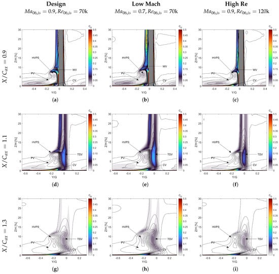
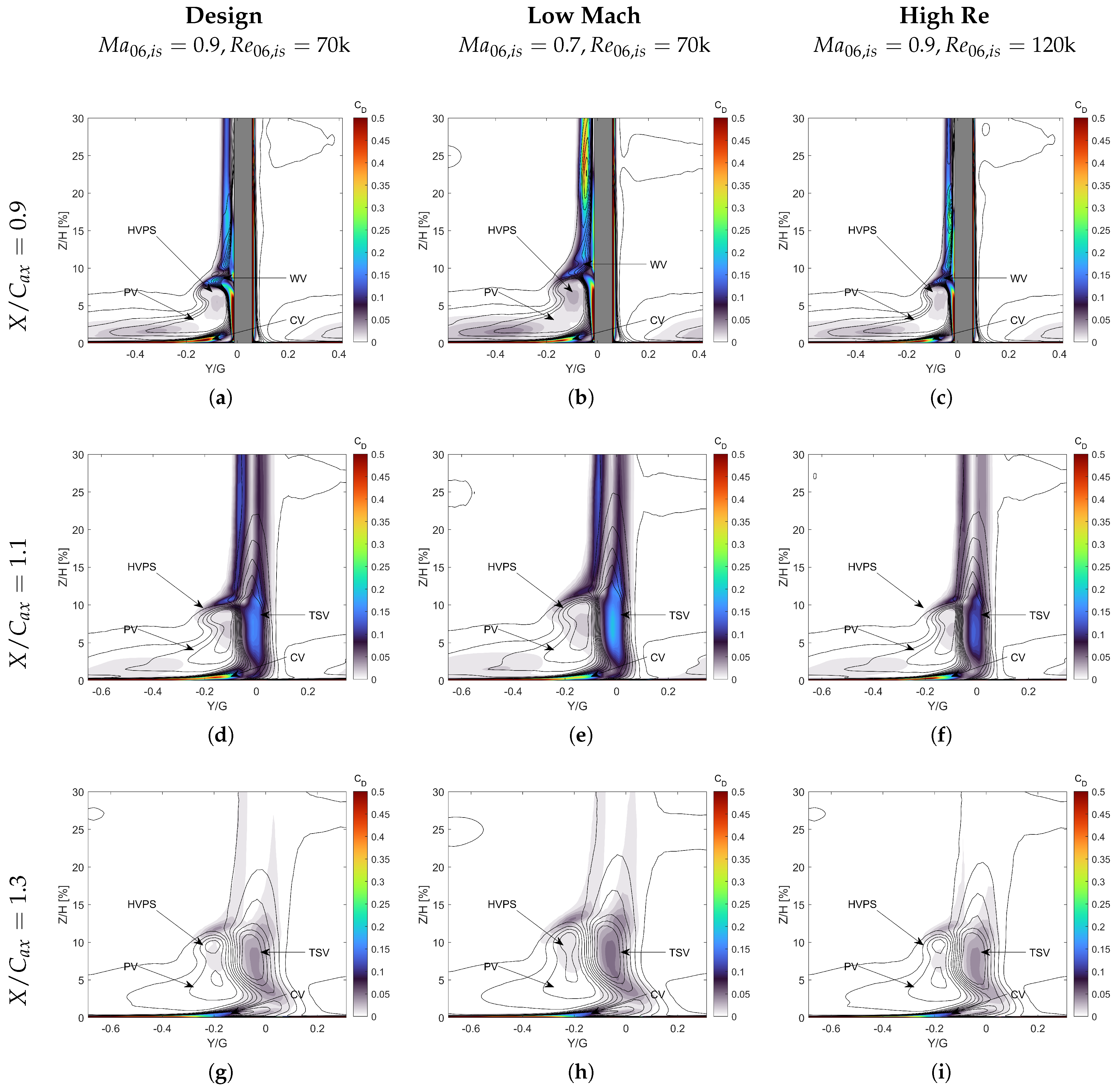
The origin of the increased losses in the case of low Mach and the lower losses in the case of high Reynolds after the start of the wake/secondary flow mixing losses can be addressed using the dissipation coefficient shown in Figure 20. The dissipation coefficient (Equation (7)) locally measures the amount of entropy generation due to viscous processes, namely the work of shear stresses and heat transfer.
Figure 20.
Dissipation coefficient () maps, structured as an operating-condition matrix. Rows represent axial measurement planes (), while columns denote operating flow conditions: (a,d,g) design condition (); (b,e,h) low Mach (); (c,f,i) high Re (). For the sake of clarity, contours are saturated at .
The contribution of the latter is small, though. Isolines in the plots refer to the streamwise vorticity coefficient, which allows for identifying the position of the vortex cores with respect to the loss-generation mechanism. As a first overall feature, the dissipation coefficient is mainly determined by the viscous interaction between the vortical structures generated throughout the cascade and the development of the boundary layers over the profile. At = 0.9, where the interaction between the PS and the SS flow has not started yet, different peaks of the dissipation coefficient can be identified in regions where the interaction between HVPS/WV, SCE2/WV, and SCE2 with the profile boundary layer occur. Additional losses are generated in the core of the HVPS and the boundary layer of the endwall and blade profile. Loss generation mainly occurs over the SS of the blade, both due to its thicker boundary layer compared to the PS of the blade and due to the sweep of the endwall flow in the spanwise direction. For the nominal conditions, the most prominent peaks of the dissipation coefficient are associated with the development of the endwall boundary layer, particularly the CV, and the spanwise migration of the HVPS and PV along the blade profile. While contours are saturated at 0.5 for visibility reasons, the in these regions can reach values as high as 1.1.
The additional loss regions of the SS boundary layer and the viscous interaction between the HVPS and the WV have comparable dissipation coefficients: ≈0.15. Eventually, the loss associated with the HVPS and the PV cores is marginally lower than the others, with the local value of 0.05. The low-Mach and the high-Reynolds cases clearly indicate different weights of the loss region. While the secondary flow interaction and spanwise migration still contribute to a significant amount of dissipation for the low-Mach case, an increased contribution for generating losses occurs in the SS boundary layer of the profile. The presence of a separation bubble and the interaction of the boundary layer with SCE2 leads to an increase in , which reaches a value of 0.5.
Moreover, the extent of the region associated with boundary layer losses is higher due to its increased thickness. Similarly to the nominal case, the losses associated with the PV and HVPS remain negligible, accounting for a tenth of the viscous dissipation due to secondary flows. On the other hand, at = 120,000, the dissipation coefficient retrieves a similar distribution and values compared to the nominal case. The main difference is in the interaction of WV and HVPS, where the mixing occurs on a smaller region and is less intense, with a peak of ≈ 0.12. Also, the loss generation associated with the SS boundary layer dissipation is higher (0.2 compared to 0.15 in the design point), but is confined to a smaller region.
At = 1.1, the behavior is qualitatively the same for all tested conditions. The losses occurring at a higher span (Z/H > 20%) are associated with the wake mixing, with a higher contribution from the SS. The evident peak within the cascade due to the interaction between the SS boundary layer and the secondary flows is now more uniform, even if this region still accounts for slightly higher losses than the main flow. The highest difference occurs at Z/H ≈ 10% at positive pitchwise positions. The mixing between the PS and the SS flow gives rise to an additional loss region associated with the development of the TSV. This loss region develops on the PS side of the wake and accounts for a similar dissipation as the interaction between the SCE2/WV and HVPS. For the low-Mach case, the TSV is stronger. This behavior in off-design conditions is further confirmed by Borbouse et al. [18] and Lopes et al. [52], who showed that compressibility effects suppress the suction-side open separation at high Mach numbers, fundamentally altering the secondary flow development and the downstream loss generation. This agrees with the amplification factors developed in [29] for the present configuration. Eventually, at = 120,000, the dissipation coefficient is lower in both the wake and secondary flow regions, while the interaction is nearly completely resolved.
No major differences occur at = 1.3, which is in agreement with the plot of the axial distribution of losses in Figure 19, showing that the operating condition majorly affects the initial mixing of the SS and PS boundary layers with the secondary flows.
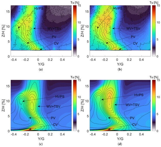
Figure 21 shows the Tu measured with PIV and the numerical predictions at PL06. Isolines of the streamwise vorticity coefficient are also reported to identify the position of high-turbulence-intensity regions. The overall agreement between the CFD simulations and PIV measurements is good, even if some differences arise due to the different flow development predicted by the RANS models. As reported in [51], PIV measurements show a more uniform flow than 5HP acquisitions and RANS predictions. It is possible to discern four different regions with high vorticity in the PIV acquisitions. A high-vorticity region is identified with the CV on the PS of the wake, while on the SS, at a low span, the PV is present. While CFD agrees with the presence of both vorticity regions, it must be highlighted that the remaining vortical structures (WV, TSV, and HVPS) predicted by RANS can be easily distinguished. They are also present in the 5HP measurements with lower overall vorticity values. In PIV measurements, the HVPS on the SS and the WV and TSV on the PS are remarkably more diffused. The viscous mixing is also the primary source of turbulence production, increasing Tu at the outlet measurement plane. CFD manages to reproduce the behavior of Tu remarkably well, as well as the turbulence intensity in the secondary flow region for both Mach conditions.
Figure 21.
Turbulence intensity at . (a) PIV , . (b) PIV , . (c) CFD , . (d) CFD , .
On the other hand, the turbulence intensity in the free stream is over-predicted. The PIV level on the side of the blade wake is around 2%, while numerical simulations predict a level of turbulence intensity of approximately 3%. This behavior is present for both operating conditions. When decreases from 0.9 to 0.7, higher turbulence levels are found, which is correctly predicted by the numerical approach. At the same time, all the structures shifted in the spanwise direction, as already discussed in Section 5.4. Because of the similarity in the secondary flow pattern, the shape of the high-turbulence region generated by the mixing process of the secondary flows is not altered by the isentropic Mach number.
The last part of this paper is dedicated to predicting endwall losses, which are compared to existing correlations in the literature. Correlations are retrieved from [29] and allow the evaluation of the endwall losses as the sum of two contributions, namely , which accounts for losses due to the endwall boundary layer dissipation, and , which accounts for the losses generated by the development of secondary flows. Following the reference, the entropy loss coefficient contributions are computed as follows:
The “AF” terms are the amplification factors related to the most relevant secondary vortex (PV, TSV, CV). The 0.0021 value is suggested by Coull [29] to appropriately weight the Marsh amplification factor (see also Marsh [53]). Finally, is the compressibility factor, defined as
The computation of the overall endwall losses of the cascade is performed according to the following splitting:
For what concerns the values of , and , they are obtained by performing a constant-area mixing calculation using the following equations:
Equation (16) defines , which represents the mixing-out losses of the incoming flow at Plane 02 relative to the midspan. Equation (17) defines , which represents the profile losses associated to the midspan entropy rise between PL02 and PL06. The various terms of the loss term are reported in Table 5, along with a comparison with the losses predicted by the correlations.
Table 5.
Loss budgeting: Comparison with existing correlations from [29]. All loss coefficients are reported in [%].
The agreement between correlations and numerical values is unsatisfactory for high-Mach conditions. In contrast, a better match with the correlations is found at low-Mach conditions, with the maximum deviation equal to 0.22%. This is consistent with the scatter obtained in [29] (0.15%). The highest difference between numerical values and correlations is found at = 120,000, where simulations predict a value for the endwall losses that is 0.45% lower than the one obtained from the correlations, which is probably induced by the flat loss profile obtained through the CFD. On the other hand, the comparison with experimental results shows a greater offset from the numerical values. The numerical simulations underestimate the experimental values for the endwall losses for all the simulated conditions. For almost all the cases, the prediction of the endwall losses is off by a factor of ≈2. Considering the shape of the energy loss coefficient shown in Figure 18, the under-prediction is mainly attributed to the loss region above the peak loss point, where numerical simulations do not yield the correct mixing between the secondary region and the midspan flow.
6. Conclusions
This paper studies the secondary flows and the effect of inlet turbulence profile specification for the linear high-speed cascade SPLEEN C1, experimentally investigated at the von Karman Institute for Fluid Dynamics during the EU-funded project SPLEEN. Numerical simulations are run using an in-house compressible flow solver developed at the Politecnico di Torino. The experimental total pressure profile and incidence angle are imposed at the inlet of the numerical domain to investigate the development of the secondary flows properly. A careful comparison between numerical predictions and experimental measurements allows for the conclusion that RANS-based transition models are valuable tools for predicting the secondary flow structure for low-pressure turbine cascades in highly compressible flows. However, flow mixing is underestimated, thus causing a clearer view of the secondary flows with respect to the experimental evidence, which includes inertial scale effects. This also leads to an over-prediction of the losses in low-span regions of the cascade, regardless of the operating conditions.
The effect of three turbulence profile specifications was investigated, specifying spanwise distributions for both the turbulence intensity and the integral length scale obtained during the experimental characterization of the rig. The profiles differ in terms of both turbulence intensity level in the boundary layer and decay upstream of the blade’s leading edge. It is shown that the inlet turbulence specification affects to a small extent the endwall flow while retaining a non-negligible effect on the secondary flow mixing. All the specified turbulence profiles correctly retrieve the pressure distribution on the endwall and guarantee a reasonable accuracy regarding the calculation of the isentropic velocity over the blade, at least for low-spanwise positions. Increased turbulence intensity along with higher integral length scales at the inlet favor the mixing of secondary structures, inducing a lower penetration in the spanwise direction of the vortices and increasing loss levels close to the hub. Finally, all specified profiles tend to overestimate the loss peak for the already mentioned underestimation of mixing between the secondary and main flow regions.
The last section of this paper investigates the cascade performance in off-design operating conditions, comparing the outlet distribution of the turbulence intensity with PIV measurements. At low Mach, the penetration of the secondary flows is higher due to the higher traveling time in the cascade. This also leads to a higher dissipation of the vorticity and, in turn, a lower mark of secondary flows on the outlet plane, along with increased endwall losses. Both profile and endwall losses are lower at high Reynolds, thanks to the associated thinner boundary layers. A comparison between the predicted endwall losses and data obtained using correlations shows good agreement at the nominal Reynolds number, while case-to-case loss variability does not find a clear correspondence in the correlations.
Author Contributions
Conceptualization, N.R., G.L., S.S., D.A.M. and S.L.; methodology, N.R. and G.L.; software, N.R., S.S. and D.A.M.; validation, N.R., G.L. and S.L.; formal analysis, N.R. and G.L.; investigation, N.R. G.L. and G.M.; resources, S.S., D.A.M. and S.L.; data curation, N.R., G.L. and G.M.; writing—original draft preparation, N.R., G.L., G.M. and S.S.; writing—review and editing, G.M., S.S., D.A.M. and S.L.; visualization, N.R., G.M. and S.S.; supervision, S.S., D.A.M. and S.L.; project administration, S.S., D.A.M. and S.L.; funding acquisition, S.S., D.A.M. and S.L. All authors have read and agreed to the published version of the manuscript.
Funding
This research received no external funding.
Data Availability Statement
The original data presented in the study are openly available in Zenodo at https://doi.org/10.5281/zenodo.8075795.
Acknowledgments
The authors acknowledge CINECA for providing computational resources under the ISCRA initiative. The authors also acknowledge the von Karman Institute for Fluid Dynamics for hosting Nicola Rosafio.
Conflicts of Interest
The authors declare no conflicts of interest.
Abbreviations
The following abbreviations are used in this manuscript:
| C | chord (m) |
| CV | corner vortex |
| streamwise vorticity coefficient | |
| G | blade pitch m |
| H | cascade height (m) |
| HV | horseshoe vortex |
| HVPS | pressure-side leg of the horseshoe vortex |
| HVSS | suction-side leg of the horseshoe vortex |
| i | incidence (°) |
| ILS | integral length scale (mm) |
| thermal conductivity (W m−1 K−1) | |
| LE | leading edge |
| LECV | leading edge corner vortex |
| LES | large eddy simulations |
| LPT | low pressure turbine |
| compressibility factor | |
| Ma | Mach number |
| total number of elements | |
| number of 2D profile elements | |
| number of spanwise layers | |
| P | static pressure |
| PS | pressure side |
| PV | passage vortex |
| RANS | Reynolds-Averaged Navier–Stokes |
| Re | Reynolds number |
| turbulence grid bar Reynolds number | |
| S | curvilinear coordinate |
| total curvilinear length | |
| SCE2 | separation-induced corner endwall vortex |
| SPV | separation-induced vortex |
| SR | stretching ratio |
| SS | suction side |
| TE | trailing edge |
| Tu | turbulence intensity |
| T | temperature (K) |
| TSV | trailing shed vortex |
| V | velocity (m s−1) |
| x | 3D coordinate |
| X | axial coordinate |
| WV | wall vortex |
| Greek Letters | |
| total pressure loss coefficient | |
| vorticity (s−1) | |
| turbulent dissipation | |
| kinematic viscosity (m2 s−1) | |
| specific heat ratio (-) | |
| density (kg m−3) | |
| shear stress tensor (kg m−1 s−2) | |
| entropy loss coefficient | |
| Superscripts and Subscripts | |
| stagnation quantity | |
| 1, 01 | referred to PL01 |
| 2, 02 | referred to PL02 |
| 6, 06 | referred to PL06 |
| ax | axial |
| in | inlet |
| mix | mixed-out |
| ms | midspan |
| prof | profile |
| sec | secondary |
| is | isentropic |
| y | pitchwise |
References
- Denton, J.D. Loss Mechanisms in Turbomachines. In Proceedings of the ASME 1993 International Gas Turbine and Aeroengine Congress and Exposition, Cincinnati, OH, USA, 24–27 May 1993. number 93-GT-435. [Google Scholar] [CrossRef] [Scilit]
- Hawtorne, W.R. Rotational flow through cascades part I. The components of vorticity. Q. J. Mech. Appl. Math. 1955, 8, 266–279. [Google Scholar] [CrossRef] [Scilit]
- Sieverding, C.H. Recent Progress in the Understanding of Basic Aspects of Secondary Flows in Turbine Blade Passages. J. Eng. Gas Turbines Power 1985, 107, 248–257. [Google Scholar] [CrossRef] [Scilit]
- Eckerle, W.A.; Langston, L.S. Horseshoe Vortex Formation Around a Cylinder. J. Turbomach. 1987, 109, 278–285. [Google Scholar] [CrossRef] [Scilit]
- Langston, L.; Nice, M.; Hooper, R. Three-Dimensional Flow Within a Turbine Cascade Passage. J. Eng. Power 1977, 99, 21. [Google Scholar] [CrossRef] [Scilit]
- Sieverding, C.H.; Van den Bosche, P. The use of coloured smoke to visualize secondary flows in a turbine-blade cascade. J. Fluid Mech. 1983, 134, 85–89. [Google Scholar] [CrossRef] [Scilit]
- Wang, H.P.; Olson, S.J.; Goldstein, R.J.; Eckert, E.R.G. Flow Visualization in a Linear Turbine Cascade of High Performance Turbine Blades. J. Turbomach. 1997, 119, 1–8. [Google Scholar] [CrossRef] [Scilit]
- Hodson, H.P.; Dominy, R.G. Three-Dimensional Flow in a Low-Pressure Turbine Cascade at Its Design Condition. J. Turbomach. 1987, 109, 177–185. [Google Scholar] [CrossRef] [Scilit]
- Hodson, H.P.; Dominy, R.G. The Off-Design Performance of a Low-Pressure Turbine Cascade. J. Turbomach. 1987, 109, 201–209. [Google Scholar] [CrossRef] [Scilit]
- Weiss, A.P.; Fottner, L. The Influence of Load Distribution on Secondary Flow in Straight Turbine Cascades. J. Turbomach. 1995, 117, 133–141. [Google Scholar] [CrossRef] [Scilit]
- Benner, M.W.; Sjolander, S.A.; Moustapha, S.H. The Influence of Leading-Edge Geometry on Secondary Losses in a Turbine Cascade at the Design Incidence. J. Turbomach. 2004, 126, 277–287. [Google Scholar] [CrossRef] [Scilit]
- Chan, J.K.K.; Yaras, M.I.; Sjolander, S.A. Interaction Between Inlet Boundary Layer, Tip-Leakage and Secondary Flows in a Low-Speed Turbine Cascade. In Proceedings of the ASME 1994 International Gas Turbine and Aeroengine Congress and Exposition, The Hague, The Netherlands, 13–16 June 1994; Volume 1: Turbomachinery; Number 94-GT-250; American Society of Mechanical Engineers: New York, NY, USA, 1994. [Google Scholar] [CrossRef] [Scilit]
- Hermanson, K.S.; Thole, K.A. Effect of Inlet Conditions on Endwall Secondary Flows. J. Propuls. Power 2000, 16, 286–296. [Google Scholar] [CrossRef] [Scilit] [PubMed]
- de la Blanco, E.R.; Hodson, H.P.; Vazquez, R.; Torre, D. Influence of the state of the inlet endwall boundary layer on the interaction between pressure surface separation and endwall flows. Proc. Inst. Mech. Eng. Part A J. Power Energy 2003, 217, 433–441. [Google Scholar] [CrossRef] [Scilit]
- Lopes, G.; Simonassi, L.; Lavagnoli, S. Impact of Unsteady Wakes on the Secondary Flows of a High-Speed Low-Pressure Turbine Cascade. Int. J. Turbomach. Propuls. Power 2023, 8, 36. [Google Scholar] [CrossRef] [Scilit]
- Lopes, G.; Lavagnoli, S. Unsteadiness in the Secondary Flows of a High-Speed Low-Pressure Turbine Cascade with Unsteady Wakes and Purge Flow. J. Turbomach. 2025, 147, 091017. [Google Scholar] [CrossRef] [Scilit]
- Lopes, G.; Simonassi, L.; Lavagnoli, S. Time-Averaged Aerodynamics of a High-Speed Low-Pressure Turbine Cascade with Cavity Purge and Unsteady Wakes. J. Turbomach. 2023, 146, 021008. [Google Scholar] [CrossRef] [Scilit]
- Borbouse, M.; Deneffe, N.; Thys, M.; Boxho, M.; Rasquin, M.; Lopes, G.; Lavagnoli, S.; Hillewaert, K. Direct Numerical Simulations of the SPLEEN cascade: A study of the impact of compressibility on transition and separation in a low-pressure turbine passage. In Proceedings of the 16th European Turbomachinery Conference (ETC16), Hannover, Germany, 24–28 March 2025. [Google Scholar] [CrossRef] [Scilit]
- Duchaine, F.; Delon, X. Assessment of Large-Eddy Simulations to Simulate a High-Speed Low-Pressure Turbine Cascade. Int. J. Turbomach. Propuls. Power 2025, 10, 21. [Google Scholar] [CrossRef] [Scilit]
- Tene Hedje, P.; Bricteux, L.; Bechane, Y.; Lavagnoli, S. Large Eddy Simulations of a High-Speed Low-Pressure Turbine Cascade at Subsonic and Transonic Mach Numbers. J. Turbomach. 2025, 147, 101010. [Google Scholar] [CrossRef] [Scilit]
- Tene Hedje, P.; Bechane, Y.; Lavagnoli, S.; Bricteux, L. Wall Resolved Large-Eddy Simulations of High-Speed Low-Pressure Turbine Cascades. In Proceedings of the ASME Turbo Expo 2023: Turbomachinery Technical Conference and Exposition, Boston, MA, USA, 26–30 June 2023; p. V13BT30A005. [Google Scholar] [CrossRef] [Scilit]
- Metti, L.; Pacciani, R.; Marco, R.; Yuan, F.; Sandberg, R.D.; Lavagnoli, S.; Marconcini, M. Multi-Fidelity Study of Secondary Flow and Transition in the SPLEEN Cascade with Endwalls. In Proceedings of the ASME Turbo Expo 2026: Turbomachinery Technical Conference and Exposition, Milan, Italy, 15–19 June 2026. [Google Scholar]
- Schenatti, A.; Bernardos, L.; Bontemps, T.; Buffaz, N.; Le Guyader, S.; Lavagnoli, S.; Laroche, E. Numerical investigation of the turbulence influence on RANS simulations in a transonic low-pressure turbine cascade. In Proceedings of the ISABE 2024, Toulouse, France, 22–27 September 2024. [Google Scholar]
- Ciorciari, R.; Kirik, I.; Niehuis, R. Effects of Unsteady Wakes on the Secondary Flows in the Linear T106 Turbine Cascade. J. Turbomach. 2014, 136, 091010. [Google Scholar] [CrossRef] [Scilit]
- Cui, J.; Nagabhushana Rao, V.; Tucker, P. Numerical investigation of secondary flows in a high-lift low pressure turbine. Int. J. Heat Fluid Flow 2017, 63, 149–157. [Google Scholar] [CrossRef] [Scilit]
- Giovannini, M.; Rubechini, F.; Marconcini, M.; Simoni, D.; Yepmo, V.; Bertini, F. Secondary Flows in LPT Cascades: Numerical and Experimental Investigation of the Impact of the Inner Part of the Boundary Layer. In Proceedings of the ASME Turbo Expo 2018: Turbomachinery Technical Conference and Exposition, Oslo, Norway, 11–15 June 2018; Volume 2B: Turbomachinery; Number GT2018-76737; American Society of Mechanical Engineers: New York, NY, USA, 2018. [Google Scholar] [CrossRef] [Scilit]
- Pichler, R.; Zhao, Y.; Sandberg, R.; Michelassi, V.; Pacciani, R.; Marconcini, M.; Arnone, A. Large-Eddy Simulation and RANS Analysis of the End-Wall Flow in a Linear Low-Pressure Turbine Cascade, Part I: Flow and Secondary Vorticity Fields Under Varying Inlet Condition. J. Turbomach. 2019, 141, 121005. [Google Scholar] [CrossRef] [Scilit]
- Marconcini, M.; Pacciani, R.; Arnone, A.; Michelassi, V.; Pichler, R.; Zhao, Y.; Sandberg, R. Large Eddy Simulation and RANS Analysis of the End-Wall Flow in a Linear Low-Pressure-Turbine Cascade—Part II: Loss Generation. J. Turbomach. 2019, 141, 051004. [Google Scholar] [CrossRef] [Scilit]
- Coull, J.D. Endwall Loss in Turbine Cascades. J. Turbomach. 2017, 139, 081004. [Google Scholar] [CrossRef] [Scilit]
- Coull, J.D.; Clark, C.J. The Effect of Inlet Conditions on Turbine Endwall Loss. J. Turbomach. 2022, 144, 101011. [Google Scholar] [CrossRef] [Scilit]
- Gisbert, F.; Cadrecha, D.; Apoita, P. Prediction of the Influence of the Inlet End-Wall Boundary Layer on the Secondary Flow of a Low Pressure Turbine Airfoil Using RANS and Large-Eddy Simulations. In Proceedings of the ASME Turbo Expo 2023: Turbomachinery Technical Conference and Exposition, Boston, MA, USA, 26–30 June 2023; Volume 13C: Turbomachinery—Deposition, Erosion, Fouling, and Icing; Design Methods and CFD Modeling for Turbomachinery; Ducts, Noise, and Component Interactions; Number GT2023-103435; American Society of Mechanical Engineers: New York, NY, USA, 2023. [Google Scholar] [CrossRef] [Scilit]
- Simonassi, L.; Lopes, G.; Gendebien, S.; Torre, A.F.M.; Patinios, M.; Lavagnoli, S.; Zeller, N.; Pintat, L. An Experimental Test Case for Transonic Low-Pressure Turbines—Part I: Rig Design, Instrumentation and Experimental Methodology. In Proceedings of the ASME Turbo Expo 2022: Turbomachinery Technical Conference and Exposition, Rotterdam, The Netherlands, 13–17 June 2022; Volume 10B: Turbomachinery—Axial Flow Turbine Aerodynamics; Deposition, Erosion, Fouling, and Icing; Radial Turbomachinery Aerodynamics; Number GT2022-81566; American Society of Mechanical Engineers: New York, NY, USA, 2022. [Google Scholar] [CrossRef] [Scilit]
- Roach, P. The generation of nearly isotropic turbulence by means of grids. Int. J. Heat Fluid Flow 1987, 8, 82–92. [Google Scholar] [CrossRef] [Scilit]
- Lopes, G.; Simonassi, L.; Torre, A.F.M.; Patinios, M.; Lavagnoli, S. An Experimental Test Case for Transonic Low-Pressure Turbines—Part 2: Cascade Aerodynamics at On- and Off-Design Reynolds and Mach Numbers. In Proceedings of the ASME Turbo Expo 2022: Turbomachinery Technical Conference and Exposition, Rotterdam, The Netherlands, 13–17 June 2022; Volume 10B: Turbomachinery—Axial Flow Turbine Aerodynamics; Deposition, Erosion, Fouling, and Icing; Radial Turbomachinery Aerodynamics; Number GT2022-82626; American Society of Mechanical Engineers: New York, NY, USA, 2022. [Google Scholar] [CrossRef] [Scilit]
- Lavagnoli, S.; Lopes, G.; Simonassi, L.; Torre, A.F.M. SPLEEN—High Speed Turbine Cascade—Test Case Database, Version v3; Zenodo: Geneva, Switzerland, 23 June 2023. [Google Scholar] [CrossRef]
- Pastorino, G.; Simonassi, L.; Lopes, G.; Boufidi, E.; Fontaneto, F.; Lavagnoli, S. Measurements of Turbulence in Compressible Low-Density Flows at the Inlet of a Transonic Linear Cascade with and Without Unsteady Wakes. In Proceedings of the ASME Turbo Expo 2023: Turbomachinery Technical Conference and Exposition, Boston, MA, USA, 26–30 June 2023; Volume 4: Controls, Diagnostics, and Instrumentation; Number GT2023-103712; American Society of Mechanical Engineers: New York, NY, USA, 2023. [Google Scholar] [CrossRef] [Scilit]
- Halby, A.; Cakir, B.O.; Da Valle, L.; Lopes, G.; Okada, M.; Lavagnoli, S. On the Application of Background Oriented Schlieren to a Transonic Low-Reynolds Turbine Cascade. J. Turbomach. 2024, 147, 051016. [Google Scholar] [CrossRef] [Scilit]
- Adami, P.; Salvadori, S.; Chana, K.S. Unsteady Heat Transfer Topics in Gas Turbine Stages Simulations. In Proceedings of the ASME Turbo Expo 2006: Power for Land, Sea, and Air, Barcelona, Spain, 8–11 May 2006; Volume 6: Turbomachinery, Parts A and B; American Society of Mechanical Engineers: New York, NY, USA, 2006; pp. 1733–1744. [Google Scholar] [CrossRef] [Scilit]
- Metti, L.; Marconcini, M.; Salvadori, S.; Anna Misul, D.; Rosafio, N.; Lopes, G.; Lavagnoli, S.; Fang, Y.; Sandberg, R.D.; Pacciani, R. The Impact of Transition and Turbulence Modeling on the SPLEEN High-Speed Low-Pressure Turbine Cascade. J. Turbomach. 2026, 148, 021011. [Google Scholar] [CrossRef] [Scilit]
- Adami, P.; Martelli, F.; Michelassi, V. Three-Dimensional Investigations for Axial Turbines by an Implicit Unstructured Multi-Block Flow Solver. In Proceedings of the ASME Turbo Expo 2000: Power for Land, Sea, and Air, Munich, Germany, 8–11 May 2000; Volume 1: Aircraft Engine; Marine; Turbomachinery; Microturbines and Small Turbomachinery; American Society of Mechanical Engineers: New York, NY, USA, 2000; p. V001T03A108. [Google Scholar] [CrossRef] [Scilit]
- Adami, P.; Belardini, E.; Martelli, F.; Michelassi, V. Unsteady Rotor/Stator Interaction: An Improved Unstructured Approach. In Proceedings of the ASME Turbo Expo 2001: Power for Land, Sea, and Air, New Orleans, LA, USA, 4–7 June 2001; Volume 1: Aircraft Engine; Marine; Turbomachinery; Microturbines and Small Turbomachinery; American Society of Mechanical Engineers: New York, NY, USA, 2001; p. V001T03A051. [Google Scholar] [CrossRef] [Scilit]
- Roe, P. Approximate Riemann solvers, parameter vectors, and difference schemes. J. Comput. Phys. 1981, 43, 357–372. [Google Scholar] [CrossRef] [Scilit]
- Ollivier-Gooch, C. High-order ENO schemes for unstructured meshes based on least-squares reconstruction. In Proceedings of the 35th Aerospace Sciences Meeting and Exhibit, Reno, NV, USA, 6–9 January 1997. [Google Scholar] [CrossRef] [Scilit][Green Version]
- Rosafio, N.; Salvadori, S.; Misul, D.A. Implementation of a high-order spatial discretization into a finite volume solver: Applications to turbomachinery test cases using an eddy-viscosity turbulence closure. Heliyon 2024, 10, e36478. [Google Scholar] [CrossRef] [Scilit] [PubMed]
- Menter, F.R. Two-equation eddy-viscosity turbulence models for engineering applications. AIAA J. 1994, 32, 1598–1605. [Google Scholar] [CrossRef] [Scilit] [PubMed]
- Langtry, R.B.; Menter, F.R. Correlation-Based Transition Modeling for Unstructured Parallelized Computational Fluid Dynamics Codes. AIAA J. 2009, 47, 2894–2906. [Google Scholar] [CrossRef] [Scilit]
- Rosafio, N.; Lopes, G.; Salvadori, S.; Lavagnoli, S.; Misul, D.A. RANS Prediction of Losses and Transition Onset in a High-Speed Low-Pressure Turbine Cascade. Energies 2023, 16, 7348. [Google Scholar] [CrossRef] [Scilit]
- Alexis, B.; Dombard, J.; Duchaine, F.; Giquel, L.; Odier, N.; Lavagnoli, S.; Lopes, G.; Simonassi, L. Analysis of rotor/stator interactions in a high-speed low-pressure turbine cascade using Large-Eddy Simulations. In Proceedings of the 15th European Conference on Turbomachinery Fluid Dynamics & Thermodynamics, Budapest, Hungary, 24–28 April 2023; Number ETC2023-257; European Turbomachinery Society: Florence, Italy, 2023. [Google Scholar] [CrossRef] [Scilit]
- Kubacki, S.; Jonak, P.; Dick, E. Evaluation of an algebraic model for laminar-to-turbulent transition on secondary flow loss in a low-pressure turbine cascade with an endwall. Int. J. Heat Fluid Flow 2019, 77, 98–112. [Google Scholar] [CrossRef] [Scilit]
- Morsbach, C.; Bergmann, M.; Tosun, A.; Klose, B.F.; Kügeler, E.; Franke, M. Large Eddy Simulation of a Low-Pressure Turbine Cascade with Turbulent End Wall Boundary Layers. Flow Turbul. Combust. 2023, 112, 165–190. [Google Scholar] [CrossRef] [Scilit]
- Okada, M.; Simonassi, L.; Lopes, G.; Lavagnoli, S. PIV measurements in a high-speed low-Reynolds low-pressure turbine cascade. J. Turbomach. 2023, 146, 031010. [Google Scholar] [CrossRef] [Scilit]
- Lopes, G.; Simonassi, L.; Torre, A.F.M.; Patinios, M.; Lavagnoli, S. Off-Design Aerodynamics of the SPLEEN C1 Cascade. Int. J. Turbomach. Propuls. Power 2026, 11, 14. [Google Scholar] [CrossRef] [Scilit]
- Marsh, H. Secondary Flow in Cascades-the Effect of Compressibility; Aeronautical Research Council: Reports and Memoranda; R. & M. No. 3778; University of Durham: Durham, UK, 1975. [Google Scholar]

Disclaimer/Publisher’s Note: The statements, opinions and data contained in all publications are solely those of the individual author(s) and contributor(s) and not of MDPI and/or the editor(s). MDPI and/or the editor(s) disclaim responsibility for any injury to people or property resulting from any ideas, methods, instructions or products referred to in the content. |
© 2026 by the authors. Published by MDPI on behalf of the European Turbomachinery Society. Licensee MDPI, Basel, Switzerland. This article is an open access article distributed under the terms and conditions of the Creative Commons Attribution (CC BY-NC-ND) license.