


Abstract
The prediction of the compressive strength (CS) for sustainable concrete reinforced with graphene nanoplatelets (GNPs) is difficult as a result of nonlinear interactions between chemical composition, dispersion state, and curing conditions. To address this, an interpretable ensemble machine learning framework is developed to provide accurate predictions of CS. The major input parameters used are sand content, graphene diameters, graphene thicknesses, and percentages of GNP to sand (GNP%; w/w), water-to-cement ratio W/C, ultrasonication period UST time (s), curing age CA day(s), while the CS (in MPa) is the target output. The random forest (RF) and XGBoost (XGB) models are incorporated into two novel metaheuristic optimization techniques, the Drawer-based optimization algorithm (DOA) and the Giant Trevally Optimizer (GTO), to enhance hyperparameter tuning and generalization. For all models, DOA XGB hybrids are the most predictive, with testing R2 values up to 0.98; RMSE of around 2.9 MPa; MAE is approximately 2.0 MPa, and well over 97% within ±20% prediction error boundaries. The explainable artificial intelligence methodologies like Shapley Additive exPlanations (SHAP), Local Interpretable Model-Agnostic Explanations (LIME), partial dependence plots, and Individual Conditional Expectation plots reveal curing age and graphene thickness as the dominant parameters. High strengths above 70 MPa are always achieved from higher curing age, w/c ratio (from 0.3 to 0.4), and graphene dosage (from 0.5 to 2.5%). A Python GUI is developed for efficient and accurate strength predictions suitable for practical applications. The proposed approach provides a robust, interpretable, and efficient alternative to extensive testing for GNP-reinforced concrete.
1. Introduction
Cementitious composites are the most widely used construction materials in civil infrastructure due to their high compressive strength, better workability, and low cost [1]. These materials underpin structures of all types, such as buildings, bridges, pavements, and industrial facilities worldwide. However, traditional concrete has mechanical and durability deficiencies despite its widespread application. It has low tensile and flexural strength, brittle failure mode, and susceptibility to cracking under mechanical loading and environmental conditioning, which greatly influence the long-term performance of the product [2,3]. Cracking promotes penetration of aggressive agents, accelerates the deterioration, and raises maintenance needs. To compensate for these drawbacks, supplementary cementitious materials (SCMs) such as fly ash, silica fume, and ground granulated blast furnace slag have been employed in other applications to enhance strength properties and durability, while also improving microstructure [4]. Although effective, these materials are mostly operative at the micro level and do not significantly improve the deficiencies of cementitious composites with respect to challenging service conditions. The development of nanotechnology has offered new prospects to improve the properties of cement-based composites by modifying the behavior of materials at the nanoscale [5]. Hydration products, pore structure, and interfacial transition zones are directly affected by nanomaterials, which contribute to the refined microstructure and enhanced mechanical properties. A variety of nanoparticles, such as carbon nanofibers, nano silica, carbon nanotubes (CNTs), micro silica, and graphene-based materials, have been included in cementitious matrices to improve strength, durability, and functionality [6,7,8,9,10]. Of these, the nanomaterials based on graphene have received a large number of research activities in recent years owing to their high flexibility, tensile strength, thermal conductivity, and specific surface area [11,12,13,14]. When introduced into the cement-based composite, GNPs accelerate hydration, increase the densification of pore structure, enhance interfacial bonding with the matrix, and bridge microcracks to improve the load transfer between fillers by strengthening crack resistance [15,16,17,18]. The multifunctional properties and their influence on concrete are presented in Figure 1.
Figure 1.
Multi-functionality of graphene nanoparticles on cementitious concrete.
Some experimental research has proved the positive effects of graphene nanoparticles on cement-based materials. Mohsen et al. [19] found that increased length and reduced particle size of graphene nanoparticles had a more pronounced effect on the compressive strength (CS) of cement paste. Chen et al. [20] studied concrete incorporated with 0.02–0.4% of graphene nanoparticles and found that the maximum increase in compressive strength was 22% when the mass percentage of graphene oxide was 0.05%. The intricate networks of interactions involved present formidable challenges to classical experimental and analytical methodologies. The experimental testing of all possible combinations of graphene percentage, mixed proportions, and curing conditions is time-consuming and unrealistic. To overcome these limitations, machine learning (ML) methods have been widely used as an effective means of predicting the properties of cementitious materials. The ML models can express hidden complex nonlinear relationships among multiple inputs without making explicit physical explanations, which would be ideally convenient for nano-modified cement systems. Strong prediction capabilities have been observed when random forest algorithms are used for predicting the strength properties of high-strength concrete [21]. The artificial neural network has been extensively applied for the prediction of CS due to its capability to learn sophisticated input–output relationships from experimental data [22]. The comparative investigations performed by Saleh et al. [23] showed that ANN yielded better predictions than did nonlinear regression (NLR), multi-expression programming (MEP), and Gaussian process for the strength of engineered cementitious composites.
The ML has also been effectively utilized for nano-modified cement-based materials. Mahmood et al. [24] used ANN and M5P tree models to predict the early-age strength of flowable cementitious materials. Mohammed et al. [25] observed that nonlinear regression and artificial intelligence approaches applied to the modeling of CS predict well for nano-clay-modified cement paste, whereas the same models have been reported with higher accuracy for nano calcium carbonate systems [26]. Similarly, Piro et al. [27] were able to predict the behavior of cement pastes containing carbon nanotubes (CNTs) with greater accuracy using ANNs than conventional regression methods. Recent works have also applied ensemble and hybrid learning methods to improve prediction stability. Adamu et al. [28] also stated that XGBoost and CatBoost models played a remarkable work for prediction on mechanical properties, water absorption, and palm fiber concrete. Vairagade et al. [29] utilized gradient boosting, deep neural networks, and optimization algorithms to improve the performance and sustainability of nano-engineered high-performance concrete. A substantiation on corresponding good performance regarding sustainable concrete was also reported upon the implementation of hybrid stacking of ensemble and deep learning models [30]. The recent progress also underscores the need for transparent and optimized machine learning approaches. Wang et al. [31] determined optimized CatBoost models that well-predicted the CS of tailings concrete, as the water binder ratio is a significant factor, by SHAP analysis.
It is noticeable that the use of an ensemble ML model has been widely used, but standalone ML models are insufficient to capture the highly nonlinear and multiscale interactions. Furthermore, several studies mentioned a lack of explainability, limiting the understanding of how input parameters influence the CS of graphene strength. The model scalability is also one of the concerns that earlier studies have not explored. By doing so, the lower cost of the experiment and optimizing the mix design can be achieved.
2. Research Significance
The existing literature reveals that researchers have tried to predict the CS of graphene nanoplatelet (GNP)-modified concrete using traditional regression and independent ML algorithms. Yet, the literature on the use of advanced ensemble ML models and recently developed metaheuristic optimization algorithms to model the intricate nanoscale interactions between GNPs and the cementitious matrix is not well established. Moreover, this dependence on specific algorithms hinders predictive accuracy, generalization, and risks the potential for overfitting. Thus, the current research tries to estimate the CS of GNP-modified concrete by employing the superior ensemble ML approaches, namely RF and XGB, in combination with two newly developed metaheuristic optimization methods, namely Drawer Optimization Algorithm (DOA) and Giant Trevally Optimizer (GTO). This investigation suggests that hybrid ML-optimization methodologies may offer tractable and reliable predictions, which have been lacking in previous studies. The working diagram of the current study is presented in Figure 2. Based on the available literature, it can be concluded that further research is required in the following scopes to establish trustworthy and accurate approaches for the prediction of CS of GNP-reinforced concrete:
Figure 2.
Working diagram of the current study.
The major findings of this study are given below:
1. The majority of reported studies on the current study problem are based on traditional regression methods or standalone ML algorithms, which makes it difficult to comprehensively address the highly nonlinear relationships between nanomaterials and concrete performance. This suggests that advanced ensemble ML methods, like RF and XGB, along with optimization methods, can improve the predictability of models and reduce overfitting.
2. The optimization of hyperparameters significantly influences the efficiency of ML models. Unlike traditional trial-and-error or simple search, the incorporation of recent metaheuristic optimizers, such as DOA and GTO, contributes to a more effective way of extracting the best parameter values, which leads to better accuracy and stability.
3. The main goal of this study is to construct and test a novel hybrid prediction framework integrating RF and XGB with DOA and GTO for predicting the CS of GNP-based concrete. The study also uses Shapley Additive exPlanations (SHAP) analysis to identify the most significant input variables (curing age, GNP thickness, and water-to-cement ratio) that balance model predictive capability and mechanism characterization for GNP-modified concrete. Further, Local Interpretable Model-Agnostic Explanations (LIME), partial dependence plots (PDP), and Individual Conditional Expectation (ICE) plots were also introduced to verify the results obtained with SHAP.
4. A Python-based GUI framework is developed where users can input the data and predict the CS, enabling researchers and engineers to make a quick decision in real time.
3. Methodology and Datasets
To develop a successful machine learning model for analyzing compressive strength behavior, the process begins with data collection (refer to Table S1). This data is then processed in detail after collection to fill in missing data, normalize entries, and otherwise prepare it for analysis. The process concludes with a comprehensive exploratory data analysis (EDA) to reveal the flow of data and the patterns it reveals. The dataset is then separated into training and testing sections to ensure proper evaluation. The ML model training comprises fine-tuning through the use of metaheuristic algorithms and cross-validation for finding the optimization of hyperparameters of employed models to enhance the accuracy and robustness. The model is then tested after it is trained with evaluation metrics. The findings are explained to draw relevant conclusions that can help in gaining an idea about the factors affecting the CS of GNPC. Every stage of this study is described via an illustration shown in Figure 2.
3.1. Data Collection and Preprocessing
For this study, the datasets were taken from the work of Fawad et al. [32] and Alyousef et al. [33], who both collected experimentally obtained data from different published sources following a thorough literature review. The data were constructed to predict the CS of concrete reinforced with graphene nanoparticle (GNP) by selecting the essential input variables according to their experimental availability and consensus from the literature. In this paper, the same datasets have been used to model CS, which consists of 172 instances with input and output information available. The inputs are classified into material properties: sand-to-cement content ratio (SC), graphene diameter (GD), graphene thickness (GT) and graphene content (GC). Likewise, the dispersion factor considered is ultrasonication time (US), and the remaining factor is curing age (CA). Proper ultrasonication helps prevent agglomeration and ensures uniform distribution, which significantly affects mechanical performance, as also reflected in the observed trends where improved dispersion leads to enhanced compressive strength. The two ranges of SC = 0 and SC = 3 represent the cement paste (no sand) and mortar mixtures with fixed sand proportion, respectively. Only samples cured in a chamber and containing graphene oxide (GrO), an amount of cement equal to unity, and all other masses expressed as a percentage of the cement mass were accounted for. However, it should be noted that certain important mix design parameters, such as cement content (kg/m3), superplasticizer dosage, and aggregate gradation, are not included in the compiled dataset. These variables significantly influence workability, hydration behavior, and strength development in practical concrete systems. Therefore, the predictive model developed in this study is constrained by the available input features, and future research should incorporate these parameters to enhance model generalization and applicability to real-world mix design. The statistical details of all input and output features are tabulated in Table 1.
Table 1.
Details of the statistical analysis of input and output parameters.
3.2. Data Analysis
Parallel coordinate plots (PCP) are a visualization technique of multivariate data, which visualizes the relation among multiple input features and the output target, as shown in Figure 3. Each vertical axis corresponds to one of these features, and the lines below each point show the normalized value (0–1) that we observed. In such a plot, it is possible to visually display many factors (SC, GD, GT, GC, W/C, US, CA, CS), as well as various characteristics of the observations on each axis. Each polyline is a single observation, which shows values of its dimensions. As a way of facilitating interpretability, color encoding, including from red to blue, is often employed to denote patterns in the noticed clusters or correlations among them. The target variable, CS are often sent to either red (high values) or blue (low values), which can help identify the relevant dependencies among important elements. The inbetween colour shows the range from 24.4 to 84.4. These are also useful for quantitative interpretation of the relationship and overall trends of multiple features. Here, the target properties, such as CS axis, are at the extreme right side and in values of 0 to 100 MPa. The red polylines denote the upper strength of CS (MPa), and the blue polylines denote the lower strength of CS (MPa). High CS exceeding 70 MPa can usually be realized by curing age over 20 days, ultrasonication time of 2–4 h, minimum W/C ratios of 0.3–0.5, moderate level graphene nanoparticles typically ranging from 0.5 to 2.5 wt%, and optimal nanoparticle thickness of between 10 and 25 nm. In contrast, the low value of CS (less than 30 MPa) is due to curing age below 5 days, and also due to a higher water–cement ratio (more than 0.6) and a high amount of graphene nanoparticles (in general, more than 4% by weight). From the above observations, it becomes clear that the main controlling key factors are significant, such as dispersion of NP, reinforcement balance, and hydration process. For improvement of the strengths in concrete, it is critical to optimize the curing period, W/C ratio, and properties of a graphene nanoparticle. The W/C ratio plays a dominant role in governing compressive strength through its direct influence on porosity and hydration mechanisms. Lower W/C ratios lead to a denser microstructure with reduced capillary voids, resulting in higher strength. Conversely, higher W/C ratios increase porosity and weaken the cement matrix. The interaction between W/C and graphene content further highlights the importance of balanced mix design, as excessive water reduces the effectiveness of nanoparticle reinforcement.
Figure 3.
Parallel coordinate plots of output with input features.
The Pearson correlation coefficient is a numerical value indicating the strength, direction, and linear relation between two quantitative variables, as shown in Figure 4. It should be noted that Pearson correlation analysis is used as an exploratory data analysis tool to quantify statistical associations within the compiled dataset. Although the input variables are independently selected in the mix design, this analysis evaluates linear relationships with compressive strength and potential interdependencies among inputs, helping to identify dominant influencing factors and possible redundancies; however, correlation does not imply causation. This coefficient is R and is determined as the covariance of two variables divided by the product of their SD’s. The sign and magnitude, therefore, provide information about both the direction and strength of this association. If the value of the coefficient is +1, then it indicates a positive relationship, and if the value is −1, then the relationship with the response variable would be an inverse strong linear relationship. In contrast, correlation values close to 0 indicate low or absent linearity. The strength and direction of the correlation are graphically depicted in heatmaps of the correlation matrices, where the color of each cell reflects the degree and sign of association between pairs of variables. The diagonal elements of the variables are always 1.0, indicating a perfect correlation with itself, as expected. The heatmap presented in Figure 4 shows that CS, which is the target variable, has high variance in terms of how much it correlates (R) with each feature. The strongest direct correlations are observed between CS vs. GT and CS vs. CA, which have correlation values of 0.48 and 0.47, respectively. Thus, an increase in GT and CA value were led to the increasing of CS of concrete and vice versa. These moderate-to-high positive correlations are seldom deterministic and should be considered in additional investigations for a common factor or even because of them. Increased graphene thickness contributes to improved crack-bridging capability, higher surface interaction with hydration products, and more effective stress transfer across the matrix. However, excessively large thickness may reduce dispersion efficiency, indicating that an optimal range is necessary for maximizing performance. Moreover, a negative correlation of −0.35 was found between the CS and W/C. The coefficient is relatively low, and it indicates a weak negative relationship between the W/C ratio and CS, as the value of the W/C ratio increases, the value of CS also decreases. For example, the correlation coefficient between CS and SC is −0.22, and between CS and GC is −0.12. They are indeed both negative; these are not comparably strong. The CS of the concrete is not closely related to either GD, with a coefficient of −0.02, or US, with 0.11 as a coefficient.
Figure 4.
Pearson plot of input and output features.
The governing parameters are strongly interdependent with CS, exhibiting both synergistic and limiting effects depending on the ranges of the governing parameters. Figure 5, as a 3D plot, depicts the two-feature interaction with respect to CS.
Figure 5.
3D plots for the impact of input on the output CS.
The subplot of Figure 5a illustrates the coupled effect of GC and W/C on CS, as CS decreases consistently with increasing W/C ratio. Until W/C = 0.4, CS decreases to approximately 40 MPa or lower. This provides evidence that when excess water is present, the matrix structure weakens owing to a higher degree of porosity and lower bonding efficiency between constituents. On the other hand, moderate GC levels have a positive effect, although their effectiveness is diminished in combination with high W/C values, indicating that appropriate water control is imperative to maximize graphene performance.
Subplot Figure 5b describes the dependence of GC on CA. For curing ages greater than around 18 to 28 days, an increase in CS can be seen, indicating that an increase in curing age increases CS. As seen at lower curing ages, the strength is rather low concerning GC, which implies incompletely hydrated material. However, with the evolution of curing, CS is better at all GC values and has performed best in moderate to high GC ranges of 3 to 6. As illustrated in subplot Figure 5c, the GD and GT are strongly positively correlated with CS over a broad parameter space. CS rises sharply with GD and GT as they both approach higher values, leading to maximum levels near the maximum CS value. It indicates that suitable particle sizes and thickness help enhance the reinforcement function and load transfer in the matrix. The uniform gradient of the surface suggests that the enhancement remains stable over a wide parameter range without fringe effects, emphasizing the necessity of moderate geometric properties.
Similarly, the subplot shown in Figure 5d illustrates the interaction between the US and GC. An increase in ultrasonication significantly improves CS, especially when US exceeds a moderate threshold. At moderate GC levels, the improvement is even greater due to better dispersion. At low US levels, CS remains relatively limited, indicating that graphene particles are not well dispersed. These results confirm the importance of ultrasonication in dispersing particle clusters and improving matrix uniformity. Likewise, the subplot presented in Figure 5e shows the combined effect of W/C and CA on CS. There is a common trend that the maximum CS values are observed at intermediate W/C ratios around 0.2 and 0.3, accompanied by extended curing time. Therefore, for lower CA, CS remains low irrespective of W/C, while for higher CA, it results in a substantial improvement in strength. On the other hand, for W/C greater than 0.5, CS experiences a steep decline at all curing ages, confirming that high water content has a detrimental effect on structural integrity.
Lastly, the subplot shown in Figure 5f demonstrates the interplay between GC and SC. CS is an increasing function of GC until it reaches a peak, at which point CC increases will either have no impact or affect CS negatively. SC at 3 has a positive effect on packing density and load transfer. High SC = 3 value decreases the CS gradually in comparison to CS at 0, which may be caused by irregularity in aggregate distribution and hindrance to bonding with the matrix. On the surface, this represents a synergistic zone where both GC and SC are in some controlled area, which results in maximum strength. Overall, Figure 5 shows that CS is very sensitive to the effects of parameter interactions, rather than the effect of just one parameter. Its optimal performance is obtained by using reasonable combinations of the above-mentioned parameters, including the graphene added amount, water-to-cement ratio, curing age, aggregate particle characteristics, and ultrasonication, as well as sand. Exceeding or undercutting these ideal ratios results in compromised strength resulting from inadequate distribution, added porosity, and/or other defects.
4. Machine Learning Models and Optimization Techniques
4.1. Ensemble Models
The RF algorithm was first introduced in 2001, which uses bagging with two key steps: (a) bootstrapping and (b) aggregating [34]. This RF operates on bagged decision trees. This technique generates multiple trees or a forest via the use of randomly allocated data to each tree [35]. It is particularly powerful for large problems, as both the rows and columns of the data matrix can be customized. It trains in parallel with such random decision trees and has a variety of hyperparameters to tune the structure, size, and randomness of each tree. In this scheme, the original data set is randomly partitioned into several subsets using bootstrap sampling. A graphical representation of the process is shown in the figure below. The RF method improves the model by selecting some features for each tree, which reduces the risk of overfitting. The best feature for each decision tree node is chosen from all the input variables, forming its left and right subtrees. This substantially helps in the generalization ability of the model. The final best prediction of the RF regression algorithm is the combination summary value or the averaged value of all outcome values resulting from these predictions for each single decision tree. The risk of overfitting was substantially minimized using an ensemble of classifiers versus a single tree, and the overall model performance increased.
The XGB algorithm is an efficient and high-performance ensemble ML algorithm, designed by Chen and Guestrin in 2016, that is based on decision tree and gradient boosting techniques [36]. This is a specialized algorithm for creating decision tree ensembles from sequential (also called gradient boosting) model fitting. This concept helps the XGB to improve the model’s performance step by step, reducing the errors from earlier rounds. There are three significant stages for developing XGB. During the first phase, prediction models are constructed for regression analysis as an ensemble of weak learners. In the second stage, XGB successively connects the newly trained tree-based models to the current model ensemble in order to minimize actual and predicted output parameter gaps and modify the loss function. The third phase is that XGB applies smart tree splitting and sophisticated random-based techniques to enhance the diversity of the tree ensemble, decreasing the value of the error in the loss function [37]. The model training routine in XGB is remarkable at minimizing an objective function to correct errors of weak learners. The objective function is a mathematical expression that the model minimizes during training, consisting of a loss function that measures prediction error and a regularization term that controls model complexity. The multiple hyperparameters, including the number of trees, learning rate, and regularization functions, have been tuned for the XGB model. The objective function used in this study is the mean squared error (MSE). This model is more optimal for complicated training situations, and becomes applicable to small-to-moderate sized dataset sets because of its ability to process quickly and handle nonlinear interactions along with bias reduction through boosting. The detailed pictorial representation of both RF and XGB is presented in Figure 6.
Figure 6.
Working process: (a) RF algorithm, (b) XGB algorithm.
4.2. Metaheuristic Algorithm
4.2.1. Giant Trevally Optimization (GTO)
The Giant Trevally Optimizer (GTO), introduced by Sadeeq and Abdulazeez in 2022, is a newly developed metaheuristic optimization algorithm modeled on the hunting behavior of the giant trevally fish [38]. It begins by randomly generating an initial population of candidate solutions called giant trevallies [39]. Each individual in this population represents a feasible solution vector for the optimization, collectively forming the population matrix of the algorithm. The detailed working process and the mathematical foundation of GTO models are well established and are presented in [38,39] with detailed exploration and exploitation strategies of metaheuristics algorithms. The pseudocode explanation of GTO is presented in Algorithm 1.
| Algorithm 1. Giant Trevally Optimizer |
|
4.2.2. Drawer Optimization (DA)
The Drawer Algorithm, developed by Dehghani and Leiva in 2023, takes its primary inspiration from simulating the process of selecting objects from a cupboard’s drawers to form an optimal combination [40]. In the DA, it is assumed that multiple drawers exist, each containing several objects. One object must be selected from each drawer to form a valid combination. Choosing suitable objects from all drawers is an optimization task that inspires the algorithm’s design. The population of the algorithm is represented as a matrix, where each row corresponds to a candidate solution and each column represents a drawer. The complete working methodology, along with the mathematical foundation of the Dais, is well established in the study of Dehgani and Leiva [40]. The detailed pseudocode of DA is presented in Algorithm 2.
| Algorithm 2. Pseudocode of the Drawer Algorithm (DA) |
|
5. Model Building and Cross-Validation
Two ensemble learning algorithms, RF and XGB, were employed for prediction modeling in this study. The models were selected due to their ability to deal with nonlinear relationships, the interplay between variables, and noise in structured data. Finally, to improve their predictive value, the optimization of hyperparameters was implemented using metaheuristic algorithms. Two state-of-the-art metaheuristic algorithms, namely GTO and DOA, were combined with RF and XGB to develop four hybrid models (GTO-RF, GTO-XGB, DOA-RF, and DOA-XGB). Table 2 lists adopted hyperparameters for the study. All the metaheuristics were run with a population of 20, considering up to 100 iterations. The tuning focused on important model parameters, including n_estimators, max_depth, and max_features for RF, while XGB has features like n_estimators, max_depth, and learning_rate. The hyperparameters n_estimators and max_depth play a critical role in controlling the performance of ensemble models. The n_estimators parameter defines the number of trees in the ensemble, influencing model stability and variance reduction, while max_depth controls the complexity of individual trees and the ability to capture nonlinear relationships. Considering the relatively moderate-sized dataset of 172 samples, these parameters were carefully optimized using metaheuristic algorithms to avoid overfitting while maintaining predictive accuracy. Moderate values were selected to ensure a balance between model complexity and generalization capability.
Table 2.
List of hyperparameters details adopted in the study.
After partitioning the dataset, the division was into training (80%) and testing (20%) data. The optimization objective was defined exclusively on the training dataset. Five-fold cross-validation (CV) was used only in the training set, serving as a measure of internal adherence of the models. The test set was reserved for final unseen evaluation. The training samples were divided into five equal parts, in which one-fold was used as the testing set once, while the rest were used for training. The dataset interchange ensures that the models are trained and validated every time for five distributions. Cross-validation gave a better general estimate of how the model would perform than a simple holdout validation and acted as a safety check for overfitting during the search for the optimal hyperparameters [41]. The utilization of metaheuristic tuning and cross-validation in the model selection enhanced the generalization potential of configurations that were well-tuned across different data partitions and, therefore, more robust as final models when applied to new predictions.
6. Performance Metrics
A comprehensive evaluation of the model’s effectiveness during training and test datasets is crucial before implementation. Evaluating the model’s performance before its deployment is an important step for confirming that it works efficiently across different datasets [42]. This evaluation work aids in confirming that the model is not just optimized for specific training data but is also capable of generalizing to various new, unseen data, which is important for robust real-world applications. To obtain this, an array of various statistical metrics is used to estimate the model’s accuracy, efficiency, consistency, and overall predictive power. In this investigation, five statistical parameters are used for the evaluation of the models, which are presented in Equations (1)–(6). These statistical metrics are the coefficient of determination (R2), root mean square error (RMSE), mean absolute error (MAE), A10 index, Willmott’s index of agreement (WI), and Nash–Sutcliffe efficiency (NS). The A10 index represents the proportion of predictions whose relative error lies within ±10% of the actual values, and is used to evaluate model accuracy in terms of acceptable prediction bounds. The use of these statistical performance metrics during the evaluation steps helps to identify various potential shortcomings that are present in the model’s predictive capabilities.
where yi = ith actual value; = ith predicted value; = mean of the predicted value; I = Indicator function, =1 if true, 0 if false; N = total no of samples. The R2 and NS in Equations (1) and (6), having the same formulae, are considered different because R2 measures variance explained in statistical regression, whereas NS evaluates predictive efficiency relative to the mean in model performance contexts.
7. Results and Discussion
7.1. Comparison of Predictions of Different ML Models
In this study, four hybrid algorithms, namely GTO-RF, GTO-XGB, DOA-RF, and DOA-XGB, were used for the prediction of CS of GNPs. The various results are obtained from training and testing sets. The resultant performance metrics obtained for training and testing data for various hybrid models are presented in Table 3 and Table 4, respectively. The result of the analysis indicates that DOA-XGB performs best on the training set, achieving an R2 of 0.999, RMSE of 0.0021, MAE of 0.0016, WI of 1, and NS of 0.999. On the other hand, DOA-XGB shows the highest performance on the testing set, with an R2 of 0.9728, RMSE of 2.935, MAE of 2.0618, WI of 0.9931, and NS of 0.9728. Although all models showed strong performance on both training and testing data sets, GTO-RF had the lowest performance in the testing phase, with an R2 of 0.926, RMSE of 4.8399, MAE of 3.9482, WI of 0.9799, and NS of 0.9262. It is important to note that the extremely low training RMSE values observed for boosting-based models are a consequence of their high approximation capability and do not represent generalization performance. In such cases, the ratio between testing and training errors becomes numerically inflated and is not a meaningful indicator of model validity. Therefore, model performance is primarily assessed based on testing and cross-validation errors. The obtained testing RMSE values (≈2.9–4.8 MPa), when compared to the dataset standard deviation (≈19 MPa), indicate acceptable predictive accuracy.
Table 3.
Performance evaluation of the models during the training phase.
Table 4.
Performance evaluation of the models during the testing phase.
The A10 index is also present in the tables showing DOA-XGB of 0.0002 and 0.198 for the training and testing sets, respectively. The error distribution as presented in the actual vs. predicted graph, illustrated in Figure 7 and Figure 8, indicates that the hybrid XGB algorithms with both NIAs are more effective, with errors within a ±20% range. The A10 index represents the proportion of predictions within ±10% error and does not explicitly identify outliers; instead, outliers are visually indicated in Figure 7 and Figure 8 as points lying outside the ±20% error bounds.
Figure 7.
Actual vs. predicted plots of the various employed models in training sets.
Figure 8.
Actual vs. predicted plots of the various employed models in testing sets.
Each subplot includes a solid 45° diagonal line indicating a perfect agreement between model predictions and target values. It also consists of two dotted lines marking a ±20% error margin around this 1:1 reference. Additionally, a dashed black line reflecting the best linear fit through the observed data points provides an alternative perspective or insight into systematic trends, such as consistent over- or under-prediction.
In the results of the training set, which are presented in Figure 7 given below, the XGBoost (XGB)-based methods, namely GTO-XGB and DOA-XGB, show a tighter clustering along the diagonal when compared to the results obtained from the RF-based method, namely GTO-RF and DOA-RF. For example, particularly for moderate to high CS values of greater than or equal to 40 MPa, these results lead to smaller residuals and a greater proportion of predictions falling within ±20% of the measured values of CS. The DOA-XGB model shows a minimal dispersion across the entire range of strength, displaying its strong capability of learning the relationships within the training data. Over 97% of DOA-XGB predictions fall within a ±20% error band, indicating that the model captures the overall trends of the dataset within an acceptable engineering tolerance. However, this metric alone does not represent model generalization or robustness, and therefore should be interpreted together with testing and cross-validation performance.
Compared with XGB-based methods, RF-based methods, namely GTO-RF and DOA-RF, effectively predict the robust mean trend. However, for some data points, particularly those data points having a value of strength above 60 MPa, deviate beyond the ±20% range of the predicted values. The best-fit dashed line as presented in each subplot of the above figure remains fairly close to the ideal 45° line, which particularly suggests a minimal biased offset, which means that the slope is either significantly below or above unity.
In the results of the test set, which are presented in Figure 8, the XGB-based methods, namely GTO-XGB and DOA-XGB, show a tighter clustering along the diagonal when compared to the results obtained from the RF-based method, namely GTO-RF and DOA-RF. For example, particularly for moderate to high CS values of greater than or equal to 40 MPa, this result leads to smaller residuals and a greater proportion of predictions fall within ±20% of the measured values of CS. The DOA-XGB model shows a minimal dispersion across the entire range of strength, displaying its strong capability of learning the relationships within the training data.
In comparison to the XGB-based methods, RF- based methods, namely GTO-RF and DOA-RF, demonstrate the prediction of the robust mean trend effectively. However, for some data points, particularly those data points having a value of strength above 60 MPa, deviate beyond the ±20% range of the predicted values. The best-fit dashed line as presented in each subplot of the above figure remains fairly close to the ideal 45° line, which particularly suggests a minimal biased offset, which means that the slope is either significantly below or above unity.
7.2. Visualization of Results
7.2.1. Convergence Curve
This plot’s convergence curve represents how the values of each variable stabilize over successive iterations during an optimization process, as shown in Figure 9. The plot presented the point where the curve shows a steep initial drop followed by the gradual flattening as the solution converges. The plateau indicates that subsequent iterations lead to minimal improvements, which suggests that the process has reached an optimal or sufficiently good solution. The efficiency of the algorithm or the methodology used for generating the curve is reflected by the slope and the point at which the curve flattens. Generally, a more efficient model flattens out faster. The plot presented in Figure 9 illustrates the convergence curve showing the graph of squared error (MSE) across 100 iterations for four hybridized models, which are developed by combining an RF and XGB algorithms with a pair of GTO and DOA methods. In the case of the GTO-RF model, which is represented by the red curve, and the DOA-RF model, which is represented by the blue curve, the curves start from near 24–25 MSE and then stabilize in the mid to low 23 range, with little improvement seen over the iterations. Whereas the GTO-XGB model is represented by the green curve and the DOA-XGB model is represented by the purple curve, the curves start around 13–14 MSE and then decrease consistently, with DOA-XGB quickly superior to GTO-XGB, then reaching and maintaining a convergence point at around nine MSE after approximately the 10th iteration. XGB-based primarily, the DOA-XGB attains superior predictive accuracy when compared with the result of the RF, which is demonstrated by the sharp decline and lower terminal value of these XGB-based models.
Figure 9.
Convergence curve of all the employed models.
7.2.2. Regression Error Characteristics Curve
The Regression error characteristics (REC) curve is an important tool for evaluating the performance of regression models. It displayed the relation between absolute deviations (error margin) on the x-axis and the ratio of predictions (accuracy) that are within this error range on the y-axis [43]. When plotting this curve, it is possible to determine what fraction of the predictions are within a given error threshold (ε) for each set of calibration data points. The models with higher REC curves perform better, since more of their predictions are below the specified error threshold, as indicated in Figure 10. The area under the curve (AUC) measures this performance, where a higher AUC implies that the model generally makes lower predictive errors across the risk spectrum. ROC curves and AUC values of the four ML models (GTO-RF, DOA-RF, GTO-XGB, and DOA-XGB) are provided in the plots. The training performance is demonstrated in panel (a), and the testing performance of models with generalization is shown in panel (b). The GTO-XGB models and the DOA-RF models are tuned for the RF and XGB using two different optimization methods. AUC provides an overall measure of prediction accuracy, with values close to 1.0 indicating better predictions holding both on average and also in absolute terms.
Figure 10.
REC curve: (a) training set, (b) testing set.
In the training phase, as shown in Figure 10a, the associated values of AUC are 0.8125, 0.8143, 0.9934, and 0.9934 for four models: GTO-RF, DOA-RF, GTO-XGB, and DOA-XGB, respectively. This is the observation as well as evidence that XGBoost models are better than RF models, with an AUC of 0.9934, which implies almost all training predictions lie in a very narrow absolute distance. Anyway, the small difference between GTO-XGB and DOA-XGB indicates that under the optimization techniques used, there are nearly similar advantages in terms of improved training accuracy. RF-based models, on the other hand, have only moderate performance with an AUC of around 0.1 and a large prediction variance. The mechanistic result is that the marginal AUC difference between the GTO-RF and the DOA-RF, which is 0.0018, implies that optimization does not provide a significant improvement on training RF models. This trend shows an important contrast between RF and XGB models. Although XGB models can easily capture complex patterns via learning from past prediction data, RF models perform very well in terms of accuracy and also generate some extreme mistakes under the prediction condition.
In the testing, a reduction in AUC values for all models is clear in Figure 10b, which indicates an increase in predictive errors for unknown data. The best and lowest models in terms of AUC are DOA-XGB and GTO-XGB with 0.8452 and 0.8262, respectively, and DOARF and GTO-RF with 0.7086 and 0.7076 AUC values, respectively. The difference in training versus testing results is, however, much less than for XGBoost models (AUC falls from 0.993 during training to 0.8452 during testing, a fact that suggests that overfitting in the final evaluation occurred to some extent). The RF model exhibits a greater but more wholesome fall of about 0.10 in the AUC set and overall safe and independent prediction. From the perspective of XGBoost models, DOAXGB has stronger generalization ability than GTO-XGB in the test phase, which implies that the DOA optimization enhances predictive robustness based on valid out-of-sample data. This causes RF-based models to be so generic and untrustworthy that they follow the performance drop when datasets are different, even in more intricate regression problems.
8. Model Explainability
8.1. SHAP Plots
SHAP (Shapley Additive exPlanations) is a game-theoretic method for interpreting machine learning model predictions [44]. It is based on the notion of Shapley values, treating each feature of the model as, in a sense, a “player” in a cooperative game, and the final prediction of the model is the “payout,” which has to be fairly divided among the players. SHAP tells how much each feature pushes the prediction up or pulls it down, from the baseline, which is usually the average prediction. This method has gained a lot of popularity for explainable AI as it gives one a measure of feature importance and a signed contribution, i.e., to what extent the feature is increasing or decreasing the predicted outcome [45,46,47].
The feature importance plot, as presented in Figure 11, shows the horizontal axis with the mean absolute SHAP value for each feature, which measures the average magnitude of each feature’s contribution to the model’s predictions. The plot shows the highest mean absolute value of SHAP for GT, which is approximately 8.90, followed by CA and GD with values approximately 7.09 and 5.76, respectively. These relatively higher values imply that these three predictors tend to have stronger effects on predicting CS relative to other predictors. Whereas W/C, GC, US, and SC, with mean absolute SHAP values of 2.60, 1.95, 0.56, and 0.45, respectively, show that these four predictors tend to have weaker effects on predicting the final results. These results show that the output of the model is primarily impacted by three predictors, namely GT, CA, and GD, while the other features have lower impacts on the output throughout the dataset.
Figure 11.
SHAP feature importance plot.
The violin (beeswarm) SHAP summary plot, as presented in Figure 12, provides a fine-grain view of each feature’s spread of SHAP values across individual instances. The color axis presented in the right part corresponds to feature magnitudes, where blue color represents lower values, and pink represents higher values. As an example, “GT” covers the range of about −35 to +20 on the SHAP scale. This result indicates that for certain observations, particularly those with low GT values denoted by blue color, there is a large negative contribution to the prediction. Whereas, at higher GT, denoted by pink color, there tends to be a positive push in the prediction. Likewise, “CA” is spread out in the range of about −20 to +10, which shows that, accordingly, high and low CA can significantly diminish, as well as including the model’s output depending on the data point. As a whole, the distributions enshrined herein emphasize the variability (spread along the x-axis) and direction (positive or negative) of each feature’s influence, providing a well-rounded overview of how input feature marginal values change model predictions in disparate contexts.
Figure 12.
SHAP summary plot.
The end predicted outcome of the force plot, as presented in Figure 13, predicts the outcome of about 21.40, with how certain features (listed with their values, i.e., “GT = 2.5” and “CA = 1.0”) push that prediction up or down from a starting reference point. The pink part to the left signifies a prediction that pulls it in a positive direction, and the blue parts extending rightwards are how other features (“GD = 6.0,” “GC = 0.1,” etc.) counteract or lessen that boost. These contributions for each feature add up to the final value of 21.40. In short, “GT” and “CA” bump the model’s output up from the baseline; “GD” and “GC” push it down, settling at an overall 21.40.
Figure 13.
SHAP force plot.
A SHAP decision plot is a powerful, informative visualization that illustrates how individual features contribute to the final predicted value in a stepwise manner across multiple data instances simultaneously. The vertical axis often displays the individual features in the order in which they were applied by the model or in an order chosen for clarity. The model output value is displayed on the horizontal axis. In a SHAP decision plot, each line represents a single row of data or observation that is being passed through the model. The individual lines begin with a baseline prediction, which is usually the overall mean output of the model across the entire training set, and then shift towards the left or right as each of the features gives up its contribution in SHAP value. In the plot presented in Figure 14, the x-axis represents predicted scores, which range approximately from 0 to 90, with some of the predictions falling within the 10–20 range, while other predictions extend anywhere around 80–90+, depending on the data. It is to be noted that how each line colored from light blue to pink/purple bends sharply for specific features, representing a strong positive or negative SHAP contribution for those specific observations. The clustering of the majority of the lines around the lower output values of around 30–40 suggests that multiple features collectively lower the prediction of the model. When the lines spread out over a wider range of higher output values, which is above 60–70, it signifies that those features work collectively to improve the predictions. This visualization technique efficiently demonstrates how various features interact to impact the outcomes of the model across varying data instances.
Figure 14.
SHAP decision plot.
The SHAP interaction plots presented in Figure 15 explain the different relationships between inputs and outputs. In the first subplot, which is on the top-left, provide the plot of SHAP value against SC, where the SC feature varies roughly from 0.0 to 3.0 on the x-axis and its respective SHAP values stretch from approximately −1.5 up to +2.0 on the y-axis. The color corresponds to W/C values approximately in the range of 0.30 to 0.70, signifying blue and pink colors, respectively. Each plot shows the average SHAP value versus SC. As expected, lower values of SC, which range from approximately 0.0 to 0.5, are normally related to modest positive SHAP contributions, which are between 0.0 and +2.0, generally when the W/C is in the lower range, as depicted by the blue color. However, as SC increases in the range between 2.0 and 3.0, a shift happens, with specific points dropping into the negative SHAP space positioned around the value of −1, particularly when W/C approaches a higher value equal to 0.70, represented by pink color. This result suggested that the higher SC value, along with increased W/C, causes a negative impact on the model’s prediction.
Figure 15.
SHAP interaction plots.
The similar characteristics can be seen at the top-middle subplot showing the plot of SHAP value against GD, where GD varies from approximately 0 to 50 on the x-axis and its respective SHAP values vary from −10 to +10 on the y-axis. The color corresponding to GC varies from 0.2 to 1 and is represented by blue and pink color respectively. From the plot, it is observed that most of the cases have moderately negative SHAP values of around −10 to −5 when GD is less than a rough threshold of 10–15, but SHAP values start to be more positive with values above +5 when GD approaches 30 or 40. This implies a tipping point after which increased GD causes the model’s predictions to gain strength.
The top-right subplot shows the plot of SHAP value against GT, which includes a range of GT values from roughly 0 to 25 on the x-axis and respective SHAP values span approximately from −30 to +10 on the y-axis, and the color indicates W/C from around 0.30 to 0.70, signifying blue and pink colors, respectively. Noticeably, when GT is under five, there exists a cluster of high positive SHAP points (greater than +5). When GT increases to around 10–15, the SHAP contributions can be as negative as −30 for certain observations, revealing a drastic change in how GT impacts the model as it crosses the threshold.
The left subplot of the middle row shows the plot of SHAP value against GC, which displays GC values from 0.0 to 6.0 on the x-axis with respective SHAP values spanning approximately from −8.0 to +6.0 on the y-axis, and the color corresponds to GT, which varies from 1 to 10 as represented by blue and pink colors, respectively. As most points are clustered in the area when GC is between 0.0 and 2.0, more values go as high as +6.0 or as low as −6.0, suggesting a potential nonlinear effect of GC for these measures on the model.
The middle subplot of the middle row shows the plot of SHAP value against W/C, which displays W/C values from 0.2 to 0.7 on the x-axis with respective SHAP values spanning approximately from −15 to +5 on the y-axis, and the color corresponds to GD, which varies from 1 to 10 as represented by blue and pink colors, respectively. Here, it is observed that when W/C is less than 0.35–0.40, SHAP values drop sharply down to a level of −15, and when W/C is approximately between 0.50 and 0.60, the contributions are more or less close to zero or are positive. Here, it is assumed that the most negative W/C influence is observed in the lower W/C range.
The right subplot of the middle row shows the plot of SHAP value against US with US on the x-axis ranging from 0.0 to 3.0 and respective SHAP values on the y-axis ranging from around −0.5 to +2.5, and colored by CA with values ranging from 5 to 25 as represented by blue and pink colors. The vast majority of points here lie in the 0.0 to 1.0 range on the US axis and yield SHAP values close to 0 or +1.0, while higher levels of US between 2.0 and 3.0 are paired with higher positive SHAP values and an increasing proportion of larger positive SHAP greater than or equal to +2.0, particularly at higher CA levels of more than 20 when they are also present.
Lastly, the subplot presented in the bottom-left shows the plot of SHAP value against CA, where CA varies between 0.0 and 25.0 on the x-axis and respective SHAP values between −15 and +8 on the y-axis, with color once again representing GT from approximately 1.0 to 10.0 as represented by blue and pink colors, respectively. When CA is low (≤5 days), the SHAP values show a wide spread, ranging from approximately −15 to +5. However, after CA reaches 15/20 days, the model demonstrates a significantly stronger positive impact, indicating that it is particularly sensitive to a higher range of CA.
Overall, the aforementioned numerous SHAP plots not only confirm the model’s predictive power but also agree with known material behavior, thereby further reinforcing the physical reliability of the findings. For instance, CA is the major factor governing the degree of hydration reactions, resulting in densification of microstructure and consequent increase in strength. The thickness of graphene also affects the crack-bridging effect and stress transfer inside the matrix. Also, the water-to-cement ratio is linked with porosity and pore connectivity; lower ratios create a denser matrix and higher strength.
8.2. LIME Plots
LIME (Local Interpretable Model-Agnostic Explanations) is a technique designed to interpret how a complex black-box model arrives at a certain specific prediction for a particular data point [48]. This method works by generating small perturbations in the feature space around the instance of interest and retrieving the predictions of the model from the black-box model. It then fits a simpler, often linear model to those local perturbations. This local surrogate essentially displays the point-wise contribution, which is either positive or negative, of each feature in influencing the prediction of the black-box model relative to a neutral baseline. Because it is trained in the vicinity of the instance of interest, LIME can provide an interpretation that is both model-agnostic and instance-specific [49].
From the LIME plot presented in Figure 16, it was observed that the model predicted the value for one observation to be 18.21, with the global minimum prediction value and global maximum prediction of around 12.58 and 89.50, respectively. The stacked bars that are illustrated in the above plot show how the features affect the prediction of the local surrogate model relative to a baseline. The blue bars, which are on the negative side, decrease the final prediction, while the orange bars, which are on the positive side relative to baseline, increase the final prediction. The feature CA ≤ 7.00 has a negative contribution of 16.28, meaning that if this bin (≤7.00) were not in CA, the local model output would be able to go up to 16 points higher. Also, “GT ≤ 1.00” contributes −14.66, which is also a prominent negative influence. Meanwhile, “GD ≤ 0.55” makes a positive addition of +12.10 to the prediction again at the top to lift up the predicted value. Summing these positive and negative contributions, one gets precisely the final value 18.21, which agrees with the result of the black-box model presented in this particular example. Through examination of its contributions, domain experts can tell what features (and with which absolute values, i.e., with topological CA = 3.00, GT = 0.70, etc.), play a key role in shaping the prediction and understand how they shift the model’s output away from the baseline.
Figure 16.
LIME plots of all input features.
To sum up, the local explanations via LIME correspond to true deviations. For instance, increasing the dosage of graphene is generally beneficial when dispersion quality is good, but detrimental in the case of agglomeration. In the same manner, a lower curing age or an increased w/c ratio may also result in understrength due to either incomplete hydration or increased porosity. Such localized insights align with experimental observations and can further explain deviations in strength for certain mix conditions. Thus, LIME is suited to serve as an extension of global SHAP case-specific explanations, enriching the practical understanding of predictions made by models.
8.3. PDP and ICE Plots
The partial dependence plots (PDPs), which show the average effect of a single predictor on the model output, with all other predictors being held at typical (i.e., median/mean) values, are not only displayed as an example, but are also used to determine the average influence of a single predictor [50]. The PDPs are presented in Figure 17. For instance, the SC axis in the PD plot for SC approximately ranges between 0.0 and 3.0. At the value of SC = 0.0, the plot begins close to the expected result of 50.8. Afterward, it then showed a long-term downward trend to about 49.4 at SC = 3.0, demonstrating a net loss of approximately 1.4 units. This result shows that as the value of SC increases within the range of 0.0 to 3.0, the predicted response from the model decreases. The PD plot for GD, on the other hand, spans a wider range from GD equal to 0 to 50, and it demonstrates a decline from around 58 at GD value near zero to about 45 for GD near 50. There is a 13-point difference corresponding to the lower and higher range of the GD, which reflects a substantial negative correlation with GD. The result showed a significantly lower expected outcome at a higher value of GD. The x-axis of the PD plot for GT ranges from 0 to 25. However, the significant variation occurs at the value of GT below 10, where the partial dependency increases steeply from about 25 to around 60, showing a 35-point increment in this range. The curve then levels off beyond the GT value of 10–15, indicating that the model becomes less sensitive to GT beyond this turning point. The other features also show distinct characteristics. For example, for GC with the range varying from 0.0 to 0.4, initially increases the prediction from about 46 to a local maximum of 53 at GC nearly equal to 0.1, showing a 7-point rise. However, the trend then reverses, declining to about 49 when GC reaches 0.4. In contrast, W/C with the x-axis range from 0.20 to 0.60 follows a distinct pattern, declining to its highest value of approximately 52 at W/C = 0.25, declining to about 47 at W/C = 0.60, resulting in an overall decrease of five points. Meanwhile, US (0.0–3.0) increases by some 1.5–2 points before leveling off at around 51.25 after US = 0.5, indicating a stabilization in its influence beyond this threshold. Lastly, CA (0–25) shows a steady and continuous upward trend, starting from an initial value of around 40 at CA = 0 and progressively increasing to about 55 at CA = 25, overall yielding an increase of 15 points.
Figure 17.
PD plots of all input features.
These average relationships are shown by PDPs, while instance-level variability is displayed by the Individual Conditional Expectation (ICE) plots, as shown in Figure 18. Each observation is represented by an individual thin blue line, which also demonstrates how the predicted outcome from that observation would change if the feature of interest (for instance, GD) is simulated varying across its observed range [51,52]. When GD increases from approximately 0 to 50, some individual lines demonstrate considerable variability, with sharp declination from +10 to –30, while other lines display a gentler drop or even remain near level. The orange dashed line presented in the plot, which represents the partial dependence plot (PDP), falls somewhere in between these trends. However, the single PDP curve presented above shows an approximate 13-point drop from 58 to 45, which does not capture the wide dispersion of possible outcomes since some individual lines shift by more than 30 points, while others shift by less than 10. These ICE plots provide us with significant insights about heterogeneity. For example, in the ICE plot for SC, the PDP shows an average drop of 1.4 points as SC increased from 0 to 3. But specific ICE lines can have a sharper decrease, between 51 and 48, or change only slightly, from 50.5 to 50. These variabilities illustrate that the sensitivity of the model to a particular feature could be equally context-sensitive, as it depends on the values of all other features for each observation. Researchers can thus attain a more precise picture of the model’s behavior by integrating the use of PDP and ICE plots, which enables the detection of subgroups or outliers where the relationship between the feature in question and the prediction deviates significantly from the average trend as captured by PDP.
Figure 18.
ICE plots of all features showing data pattern.
Overall, the PDP results showed higher CS with increasing curing age CA, optimal ranges of graphene content, and water-to-cement ratio. These trends are representative of the impact that prolonged hydration and optimized nanomaterial dosing can have on improving matrix densification and mechanics. Additional variability across parameters and interactions can be observed within the ICE plots, indicating that these effects do not apply uniformly across all samples. Graphene content impact is contingent on dispersion quality and ultrasonication time, while water-to-cement ratio behavior is dependent on curing conditions. Such behavior agrees with the interacting nature of physicochemical processes in cementitious systems, as multiple interactions exist to dictate hydration, dispersion, and microstructure evolution. Thus, PDP shows the average trend, and ICE focuses on the variability due to complex interactions of materials.
9. GUI-Based Development
The development of the graphical user interface (GUI) was done in Python using an Anaconda Navigator environment for the application of the employed models. The interface graphics were created and drawn using Tkinter, a common Python GUI toolkit. The interface is developed specifically for the prediction of CS in carbon-based nanomaterials, offering a user-friendly portal to researchers and developers in graphene-enhanced cementitious composites. Multiple input fields are available in the interface for users to input values of key parameters such as sand content, diameter, and thickness of graphene nanoplatelet, GNP content, water-to-cement ratio, ultrasonication time, and curing age. The minimum and maximum values of the input fields are dynamically programmed to reduce errors in data entry. The interaction between the key input fields, labels, and buttons is done in a neat grid-based layout, ensuring clarity and simplicity. To facilitate practical usage, a brief user workflow is incorporated, where users input the required parameters, execute the prediction through a single action button, and obtain the compressive strength output instantly within the interface. The results obtained from the prediction are displayed prominently within the interface, letting users to rapidly interpret the output. An example use case is also considered, where a typical mix design with defined input parameters is entered into the GUI, and the corresponding compressive strength is predicted, demonstrating the applicability of the tool for rapid decision-making in mix design. This focuses on clear and efficient presentation, which boosts the usability of the application, resulting in a time-efficient tool for researchers and engineers who work on investigating the mechanical properties of graphene-reinforced cementitious materials. Furthermore, the GUI outputs are directly linked to the validated DOA-XGB model, and consistency of predictions has been verified against the testing dataset, confirming the reliability of the interface for practical applications. A representative screenshot of the GUI is provided in Figure 19 to illustrate its layout, functionality, and ease of interaction.
Figure 19.
Graphical user interface of the best model.
10. Limitations and Future Research Directions
While hybrid ensemble models that are optimized by state-of-the-art metaheuristics proved to be successful, some limitations in this study need to be recognized. The forecasting model significantly relies on the quality, resolution, and representativeness of the data. Although the model accurately predicted in the specific range of parameter space, it might fail to perform in the extrapolation to data in the region outside the domain, especially in the case of rare or additional material configurations that had not been included in the training. Moreover, although the metaheuristic-based algorithms, such as GTO and DOA, were able to conduct meaningful tuning of hyperparameters, they resulted in computational overhead because of the iterative evaluations and the stochastic nature, which may affect the scalability and the consistency of tuning across runs. Furthermore, interpretability methods such as SHAP, LIME, ICE, and PDP have made meaningful strides in providing transparency into the decisions that models are making, but come with methodological assumptions and limitations that may compromise the accuracy of explanations, most notably in regions of parametric feature interaction or sparsity.
So, the future work in the short term is to enlarge and diversify the dataset by extending to a variety of types of nanomaterials, mixture compositions, curing regimens, and process conditions. This will contribute to the good generalization of the model, and it will learn a more complex structure–property relationship. Moreover, multi-objective design optimization will be investigated where compressive strength has to be weighed against other crucial quantities, obtainable simultaneously, such as durability, workability, and costs. On the modeling aspect, subsequent work will incorporate uncertainty quantification approaches to account for prediction confidence and enhance decision-making in real-world scenarios. Improvements to the GUI are also envisaged, such as dynamic parameter range specification, real-time interpretability outputs, and connection to downstream lab-scale tests for feedback-based experimental design.
Future work should focus on incorporating comprehensive mix design variables, including binder content, chemical admixtures, and aggregate characteristics, to improve the robustness and practical applicability of machine learning models in concrete design. Finally, the approach will be applied to other high-performance cementitious systems to offer a generalized framework for strength prediction and explainability in advanced materials research.
11. Conclusions
This study demonstrates that ensemble machine learning models, combined with metaheuristic optimization, provide a robust and defendable solution for predicting the compressive strength of GNP-reinforced concretes. By exploring the hyperparameter space, we find that RF and XGBoost models with DOA-GTO will significantly increase model stability and generalization. The optimized hybrids outperform both standalone models by reducing the prediction error and overfitting, which indicates that the metaheuristic-based tuning process is effective in highly nonlinear material systems. Out of all trained models, the DOA XGB hybrid model achieves the highest generalization on unseen data (0.97–0.98 for testing R2 values and 2.9–4.8 MPa for RMSE and MAE of around 2). For the GTO-based XGB models, a slightly lower accuracy compared to those of ETR XGB, where both R2 range between 0.96 and 0.97 and RMSE values are beyond 3.1 MPa, in contrast to around 2.8 for ETR-XGB, as well as RF-based hybrids exhibit higher errors in general.
The feature influence analysis indicates that curing age and the thickness of graphene are major parameters influencing compressive strength. High compressive strength (over 70 MPa) is always related to curing ages higher than 20 days, W/C ratio from 0.3 to 0.4, graphene percentage of the order of 0.5 and 2.5%, and high sonication conditions are required. Interaction analysis shows that strength gains are greater than 300 MPa when the graphene content is over 3%, or the water-to-cement ratio exceeds 0.5, which indicates a high sensitivity of the model to inappropriate selection of parameters.
Explainability techniques further confirm the physical consistency of the proposed models. SHAP analysis provides the quantitative precedence of curing age, graphene thickness, and water-to-cement ratio as influential predictors, while PDP and ICE plots display non-confusing monotonic and interaction trend behaviors in the optimal range of parameter space. This local predictive phenomenon is verified at the LIME level and strengthens the credibility of model interpretability. These validated models were utilized in a Python-based GUI (graphical user interface) where they are implemented into a user-friendly tool that provides for the reliable prediction of CS with errors typically less than 3 MPa from provided inputs. In summary, the presented integrated framework of ensemble learning, DOA, and three-level GTO, explainable AI, as well as GUI-based deployment, provides a technically sound and interpretable efficient approach to reduce excessive experimental testing required for graphene nanoplatelet reinforced concrete.
Supplementary Materials
The following supporting information can be downloaded at: https://www.mdpi.com/article/10.3390/infrastructures11050146/s1. The dataset supporting the findings of this study can be found in Supplementary Material (Table S1: Dataset considered for analysis.) accompanying this article.
Author Contributions
Conceptualization, methodology, S.C.S. and M.H.; software, data curation, visualizations, S.C.S., S.A., A.D., R.P., A.G. and T.B.; formal analysis, S.C.S., A.G. and S.A.; investigation, S.C.S., M.H., B.T. and T.B.; resources, S.C.S.; validation, S.C.S., M.H., B.T., R.P. and T.B.; writing—original draft, S.C.S., M.H., B.T., S.A., A.D., R.P. and A.G.; writing—review and editing, S.C.S., M.H. and T.B.; supervision, project administration, M.H. and S.C.S.; funding acquisition, S.C.S., M.H. and T.B. All authors have read and agreed to the published version of the manuscript.
Funding
This research received no external funding.
Data Availability Statement
The data that support the findings of this study are available from the corresponding author upon reasonable request.
Conflicts of Interest
The authors declare that they have no known competing financial interest or personal relationships that could have appeared to influence the work reported in this paper.
Abbreviations
| GTO | Giant Trevally Optimizer |
| DOA | Drawer Optimization Algorithm |
| RF | Random Forest |
| XGB | Extreme Gradient Boosting |
| AUC | Area under Curve |
| SHAP | Shapley Additive exPlanations |
| LIME | Local Interpretable Model-Agnostic Explanations |
| PDP | Partial dependence plots |
| ICE | Individual Conditional Expectation |
| GUI | Graphical user interface |
| GNPs | Graphene Nanoplatelets |
| CS | Compressive Strength |
| SC | Sand Content |
| GD | Graphene Diameter |
| GT | Graphene Thickness |
| GC | Graphene Content (GC) |
| US | Ultrasonication time |
| CA | Curing Age |
| W/C | Water-to-Cement ratio |
References
- Lin, Y.; Du, H. Graphene Reinforced Cement Composites: A Review. Constr. Build. Mater. 2020, 265, 120312. [Google Scholar] [CrossRef] [Scilit]
- Han, B.; Zhang, L.; Ou, J. Smart and Multifunctional Concrete Toward Sustainable Infrastructures; Springer: Singapore, 2017. [Google Scholar]
- Junaid, T.M.; Kayali, O.; Khennane, A. Response of alkali activated low calcium fly-ash based geopolymer concrete under compressive load at elevated temperatures. Mater. Struct. 2017, 50, 87. [Google Scholar] [CrossRef] [Scilit]
- Fode, T.A.; Jande, Y.A.C.; Kivevele, T. Effects of different supplementary cementitious materials on durability and mechanical properties of cement composite—Comprehensive review. Heliyon 2023, 9, e17924. [Google Scholar] [CrossRef] [Scilit] [PubMed]
- Monteiro, H.; Moura, B.; Soares, N. Advancements in nano-enabled cement and concrete: Innovative properties and environmental implications. J. Build. Eng. 2022, 56, 104736. [Google Scholar] [CrossRef] [Scilit]
- Abdulkadir, I.; Wong, L.S.; Ean, L.W.; Murali, G.; Mohammed, B.S. A holistic review of nanomaterials in strain-hardening cementitious composites: Insights into micro- and macromechanical, deformation, smart, and durability properties. Results Eng. 2025, 25, 104099. [Google Scholar] [CrossRef] [Scilit]
- Abdalla, J.A.; Hawileh, R.A.; Bahurudeen, A.; Jittin, K.I.; Kabeer, S.A.; Thomas, B.S. Influence of synthesized nanomaterials in the strength and durability of cementitious composites. Case Stud. Constr. Mater. 2023, 18, e02197. [Google Scholar] [CrossRef] [Scilit]
- Tabish, M.; Zaheer, M.M.; Baqi, A. Effect of nano-silica on mechanical, microstructural and durability properties of cement-based materials: A review. J. Build. Eng. 2023, 65, 105676. [Google Scholar] [CrossRef] [Scilit]
- Li, H.; Zhao, Y.; Zhao, Y.; Zhang, M.; Niu, Y.; Cao, X. Advances in the Mechanism and Application of Nanoparticles in Concrete Property Modification. Inorganics 2025, 13, 305. [Google Scholar] [CrossRef] [Scilit]
- Ainomugisha, S.; Matovu, M.J.; Manga, M. Influence mechanisms of silica nanoparticles’ property enhancement in cementitious materials and their green synthesis: A critical review. Case Stud. Constr. Mater. 2024, 20, e03372. [Google Scholar] [CrossRef] [Scilit]
- Yusaf, T.; Mahamude, A.S.F.; Farhana, K.; Harun, W.S.W.; Kadirgama, K.; Ramasamy, D.; Kamarulzaman, M.K.; Subramonian, S.; Hall, S.; Dhahad, H.A. A Comprehensive Review on Graphene Nanoparticles: Preparation, Properties, and Applications. Sustainability 2022, 14, 12336. [Google Scholar] [CrossRef] [Scilit]
- Singh, S.; Hasan, M.R.; Sharma, P.; Narang, J. Graphene nanomaterials: The wondering material from synthesis to applications. Sens. Int. 2022, 3, 100190. [Google Scholar] [CrossRef] [Scilit]
- Sai T, Y.; Jagadeesh, P. Efficacy of graphene oxide-based nanomaterials in customized cement mixtures, a review of recent research trends. Hybrid Adv. 2025, 10, 100428. [Google Scholar] [CrossRef] [Scilit]
- Perala, R.S.; Chandrasekar, N.; Balaji, R.; Alexander, P.S.; Humaidi, N.Z.N.; Hwang, M.T. A comprehensive review on graphene-based materials: From synthesis to contemporary sensor applications. Mater. Sci. Eng. R Rep. 2024, 159, 100805. [Google Scholar] [CrossRef] [Scilit]
- Yang, Q.; Yang, Q.; Peng, X.; Xia, K.; Xu, B. A Review of the Effects of Nanomaterials on the Properties of Concrete. Buildings 2025, 15, 2363. [Google Scholar] [CrossRef] [Scilit]
- Liu, B.; Wang, J.; Wei, Z.; Peng, Y.; Wu, J. Damping and Microstructure of Graphene/Carbon Nanotube-Modified Cement Composites. Buildings 2025, 15, 3317. [Google Scholar] [CrossRef] [Scilit]
- Dai, J.; Wang, Y.; Luo, L.; Dong, X.; Wang, Q. Effects of graphene oxide on hydration of cement-based materials at different curing temperatures. J. Build. Eng. 2025, 111, 113268. [Google Scholar] [CrossRef] [Scilit]
- Lu, D.; Shi, X.; Zhong, J. Nano-engineering the interfacial transition zone in cement composites with graphene oxide. Constr. Build. Mater. 2022, 356, 129284. [Google Scholar] [CrossRef] [Scilit]
- Mohsen, M.O.; Taha, R.; Abu Taqa, A.; Al-Nuaimi, N.; Al-Rub, R.A.; Bani-Hani, K.A. Effect of Nanotube Geometry on the Strength and Dispersion of CNT-Cement Composites. J. Nanomater. 2017, 2017, 6927416. [Google Scholar] [CrossRef] [Scilit]
- Chen, G.; Yang, M.; Xu, L.; Zhang, Y.; Wang, Y. Graphene Nanoplatelets Impact on Concrete in Improving Freeze-Thaw Resistance. Appl. Sci. 2019, 9, 3582. [Google Scholar] [CrossRef] [Scilit]
- Farooq, F.; Nasir Amin, M.; Khan, K.; Rehan Sadiq, M.; Faisal Javed, M.; Aslam, F.; Alyousef, R. A Comparative Study of Random Forest and Genetic Engineering Programming for the Prediction of Compressive Strength of High Strength Concrete (HSC). Appl. Sci. 2020, 10, 7330. [Google Scholar] [CrossRef] [Scilit]
- Keshavarz, Z.; Torkian, H. Application of ANN and ANFIS models in determining compressive strength of concrete. J. Soft Comput. Civ. Eng. 2018, 2, 62–70. [Google Scholar] [CrossRef] [Scilit]
- Saleh, P.Y.; Jaf, D.K.I.; Abdalla, A.A.; Ahmed, H.U.; Faraj, R.H.; Mahmood, W.; Mohammed, A.S. Prediction of the compressive strength of strain hardening cement-based composites using soft computing models. Struct. Concr. 2023, 24, 6761–6777. [Google Scholar] [CrossRef] [Scilit]
- Mahmood, W.; Mohammed, A.S.; Asteris, P.G.; Ahmed, H. Soft computing technics to predict the early age compressive strength of flowable ordinary Portland cement. Soft Comput. 2023, 27, 3133–3150. [Google Scholar] [CrossRef] [Scilit]
- Mohammed, A.; Rafiq, S.; Mahmood, W.; Al Darkazali, H.; Noaman, R.; Qadir, W.; Ghafor, K. Artificial neural network and NLR techniques to predict the rheological properties and compressive strength of cement paste modified with nanoclay. Ain Shams Eng. J. 2021, 12, 1313–1328. [Google Scholar] [CrossRef] [Scilit]
- Salih, A.; Rafiq, S.; Mahmood, W.; Al Darkazali, H.; Noaman, R.; Ghafor, K.; Qadir, W. Systemic multi scale approaches to predict the flowability at various temperature and mechanical properties of cement paste modified with nanocalcium carbonate. Constr. Build. Mater. 2020, 262, 120777. [Google Scholar] [CrossRef] [Scilit]
- Piro, N.S.; Mohammed, A.S.; Hamad, S.M. Multiple Analytical Models to Evaluate the Impact of Carbon Nanotubes on the Electrical Resistivity and Compressive Strength of the Cement Paste. Sustainability 2021, 13, 12544. [Google Scholar] [CrossRef] [Scilit]
- Adamu, M.; Sapkota, S.C.; Das, S.; Saha, P.; Ibrahim, Y.E. An explainable boosting based ensemble machine learning model for predicting the properties of date palm fiber reinforced concrete. Sustain. Chem. Pharm. 2025, 44, 101949. [Google Scholar] [CrossRef] [Scilit]
- Vairagade, V.S.; Bahoria, B.V.; Isleem, H.F.; Shelke, N.; Mungle, N.P. Strength and durability predictions of ternary blended nano-engineered high-performance concrete: Application of hybrid machine learning techniques with bio-inspired optimization. Eng. Appl. Artif. Intell. 2025, 148, 110470. [Google Scholar] [CrossRef] [Scilit]
- Sapkota, S.C.; Sapkota, S.; Saini, G.; Sivenas, T.; Armaghani, D.J.; Asteris, P.G. Computational intelligence enhances compressive strength estimation of sustainable concrete using industrial waste. Struct. Concr. 2025, 27, 1160–1183. [Google Scholar] [CrossRef] [Scilit]
- Wang, Z.; Liu, S.; Liang, W.; Liu, J.; Zhou, Y.; Lei, K.; Gao, Y.; Ou, W. Predictive Modeling of Compressive Strength in Tailings Concrete Using Explainable Machine Learning Approaches. Results Eng. 2025, 27, 105516. [Google Scholar] [CrossRef] [Scilit]
- Fawad, M.; Alabduljabbar, H.; Farooq, F.; Najeh, T.; Gamil, Y.; Ahmed, B. Indirect prediction of graphene nanoplatelets reinforced cementitious composites compressive strength by using machine learning approaches. Sci. Rep. 2024, 14, 14252. [Google Scholar] [CrossRef] [Scilit]
- Alyousef, R.; Nassar, R.U.D.; Fawad, M.; Farooq, F.; Gamil, Y.; Najeh, T. Predicting the properties of concrete incorporating graphene nanoplatelets by experimental and machine learning approaches. Case Stud. Constr. Mater. 2024, 20, e03018. [Google Scholar] [CrossRef] [Scilit]
- Breiman, L. Random forests. Mach. Learn. 2001, 45, 5–32. [Google Scholar] [CrossRef] [Scilit]
- Louppe, G. Understanding random forests. From theory to practice. arXiv 2015. [Google Scholar] [CrossRef] [Scilit]
- Chen, T.; Guestrin, C. XGBoost: A scalable tree boosting system. In Proceedings of the 22nd ACM SIGKDD International Conference on Knowledge Discovery and Data Mining, San Francisco, CA, USA, 13–17 August 2016; Association for Computing Machinery: New York, NY, USA, 2016; pp. 785–794. [Google Scholar] [CrossRef] [Scilit]
- Sapkota, S.C.; Shrestha, A.; Tang, W. Metaheuristic optimized machine learning models for accurate prediction of limestone calcined clay cement compressive strength. Case Stud. Constr. Mater. 2025, 23, e05303. [Google Scholar] [CrossRef] [Scilit]
- Sadeeq, H.T.; Abdulazeez, A.M. Giant trevally optimizer (GTO). A novel metaheuristic algorithm for global optimization and challenging engineering problems. IEEE Access 2022, 10, 121615–121640. [Google Scholar] [CrossRef] [Scilit]
- Hashish, M.S.; Hasanien, H.M.; Ullah, Z.; Alkuhayli, A.; Badr, A.O. Giant Trevally Optimization Approach for Probabilistic Optimal Power Flow of Power Systems Including Renewable Energy Systems Uncertainty. Sustainability 2023, 15, 13283. [Google Scholar] [CrossRef] [Scilit]
- Trojovská, E.; Dehghani, M.; Leiva, V. Drawer Algorithm: A New Metaheuristic Approach for Solving Optimization Problems in Engineering. Biomimetics 2023, 8, 239. [Google Scholar] [CrossRef] [Scilit]
- Gorriz, J.M.; Clemente, R.M.; Segovia, F.; Ramirez, J.; Ortiz, A.; Suckling, J. Is K fold cross validation the best model selection method for machine learning. arXiv 2024. [Google Scholar] [CrossRef] [Scilit]
- Sapkota, S.C.; Sapkota, S.; Bansal, T.; Haq, M.; Al-Osta, M.A. Leveraging interpretable ensemble machine learning for predicting interfacial bond strength between normal strength concrete substrate and UHPC overlays. Arab. J. Sci. Eng. 2025, 50, 8621–8645. [Google Scholar] [CrossRef] [Scilit]
- Bi, J.; Bennett, K.P. Regression error characteristic curves. In Proceedings of the 20th International Conference on Machine Learning, Washington, DC, USA, 21–24 August 2003; AAAI Press: Menlo Park, CA, USA, 2003; pp. 43–50. [Google Scholar]
- Lundberg, S.; Lee, S.I. A unified approach to interpreting model predictions. arXiv 2017, arXiv:1705.07874. [Google Scholar] [CrossRef] [Scilit]
- Lundberg, S.M.; Erion, G.; Chen, H.; DeGrave, A.; Prutkin, J.M.; Nair, B.; Katz, R.; Himmelfarb, J.; Bansal, N.; Lee, S.I. From local explanations to global understanding with explainable AI for trees. Nat. Mach. Intell. 2020, 2, 56–67. [Google Scholar] [CrossRef] [Scilit] [PubMed]
- Noaman, M.F.; Haq, M.; Sapkota, S.C.; Khan, M.A.; Ali, K.; Kamyab, H. Prediction of Consolidation Behavior of Modified Clayey Soil Reinforced with Artificial Geo-Fibers Using Explainable Artificial Intelligence. Chemom. Intell. Lab. Syst. 2026, 271, 105654. [Google Scholar] [CrossRef] [Scilit]
- Sapkota, S.C.; Shrestha, S.; Haq, M.; Panthi, A.; Shrestha, A.; Sapkota, S.; Al-Osta, M.A.; Bansal, T. Explainable Hybridized Ensemble Model with a Metaheuristics Algorithm for the Prediction of Compressive Strength of Ultrahigh-Performance Concrete. J. Struct. Des. Constr. Pract. 2026, 31, 04026023. [Google Scholar] [CrossRef] [Scilit]
- Ribeiro, M.T.; Singh, S.; Guestrin, C. Why should I trust you? Explaining the predictions of any classifier. arXiv 2016, arXiv:1602.04938. [Google Scholar] [CrossRef] [Scilit]
- Salih, A.M.; Raisi-Estabragh, Z.; Galazzo, I.B.; Radeva, P.; Petersen, S.E.; Lekadir, K.; Menegaz, G. A perspective on explainable artificial intelligence methods: SHAP and LIME. Adv. Intell. Syst. 2025, 7, 2400304. [Google Scholar] [CrossRef] [Scilit]
- Muschalik, M.; Fumagalli, F.; Jagtani, R.; Hammer, B.; Hüllermeier, E. iPDP. On partial dependence plots in dynamic modeling scenarios. In Explainable Artificial Intelligence; Longo, L., Ed.; Communications in Computer and Information Science; Springer: Cham, Switzerland, 2023; Volume 1901, pp. 173–189. [Google Scholar] [CrossRef] [Scilit]
- Goldstein, A.; Kapelner, A.; Bleich, J.; Pitkin, E. Peeking inside the black box. Visualizing statistical learning with plots of individual conditional expectation. arXiv 2014, arXiv:1309.6392. [Google Scholar] [CrossRef] [Scilit]
- Yeh, A.; Ngo, A. Bringing a ruler into the black box: Uncovering feature impact from individual conditional expectation plots. In Machine Learning and Principles and Practice of Knowledge Discovery in Databases; Kamp, M., Koprinska, I., Bibal, A., Bouadi, T., Frenay, B., Galarraga, L., Oramas, J., Adilova, L., Krishnamurthy, Y., Kang, B., et al., Eds.; Communications in Computer and Information Science; Springer: Cham, Switzerland, 2021; Volume 1524, pp. 47–61. [Google Scholar] [CrossRef] [Scilit]
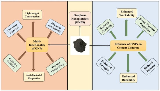
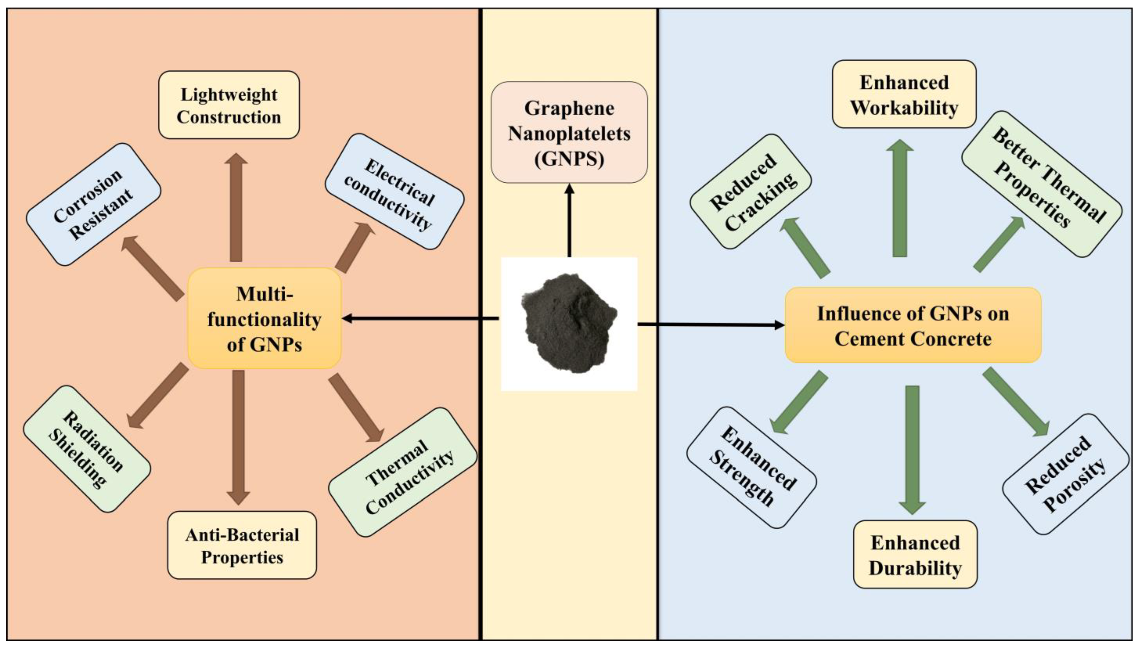
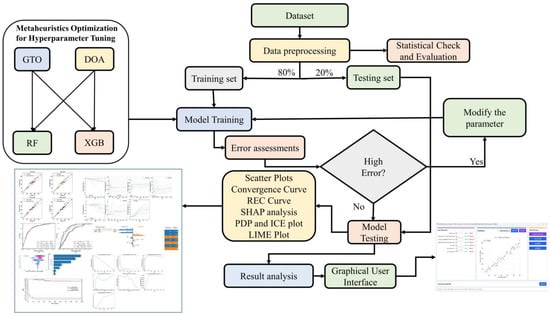
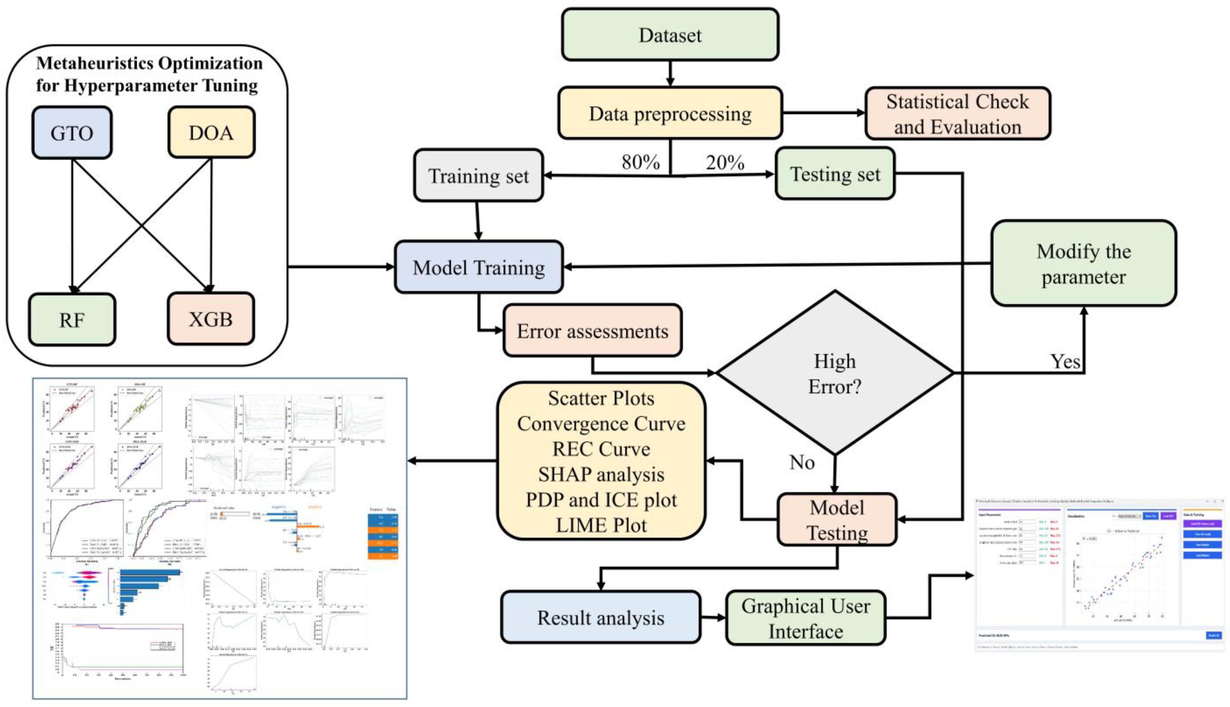
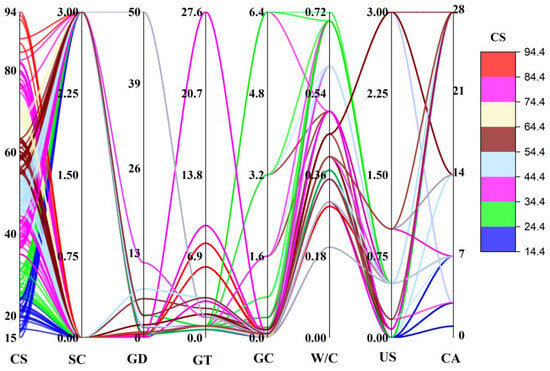
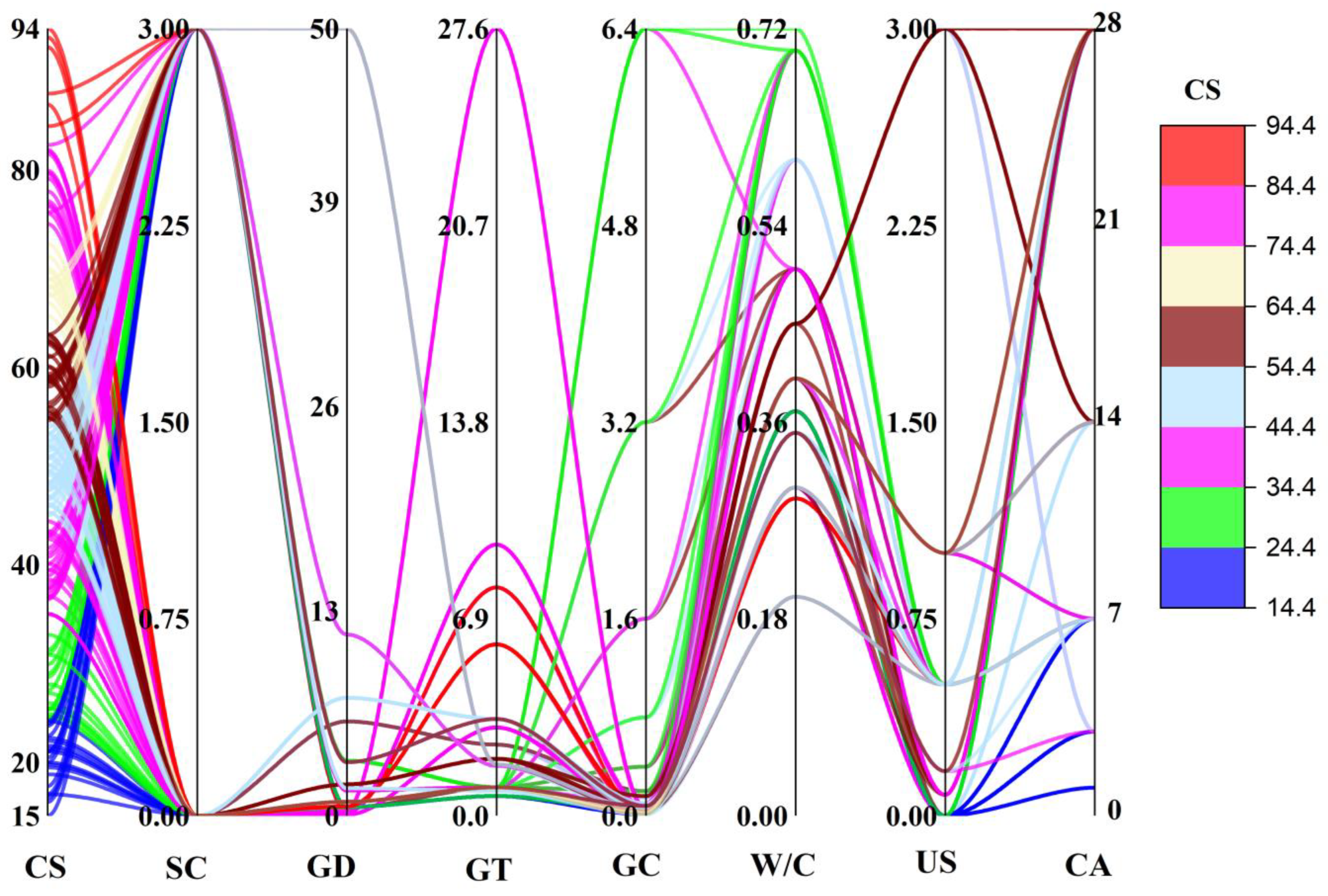
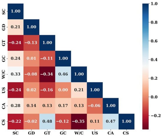
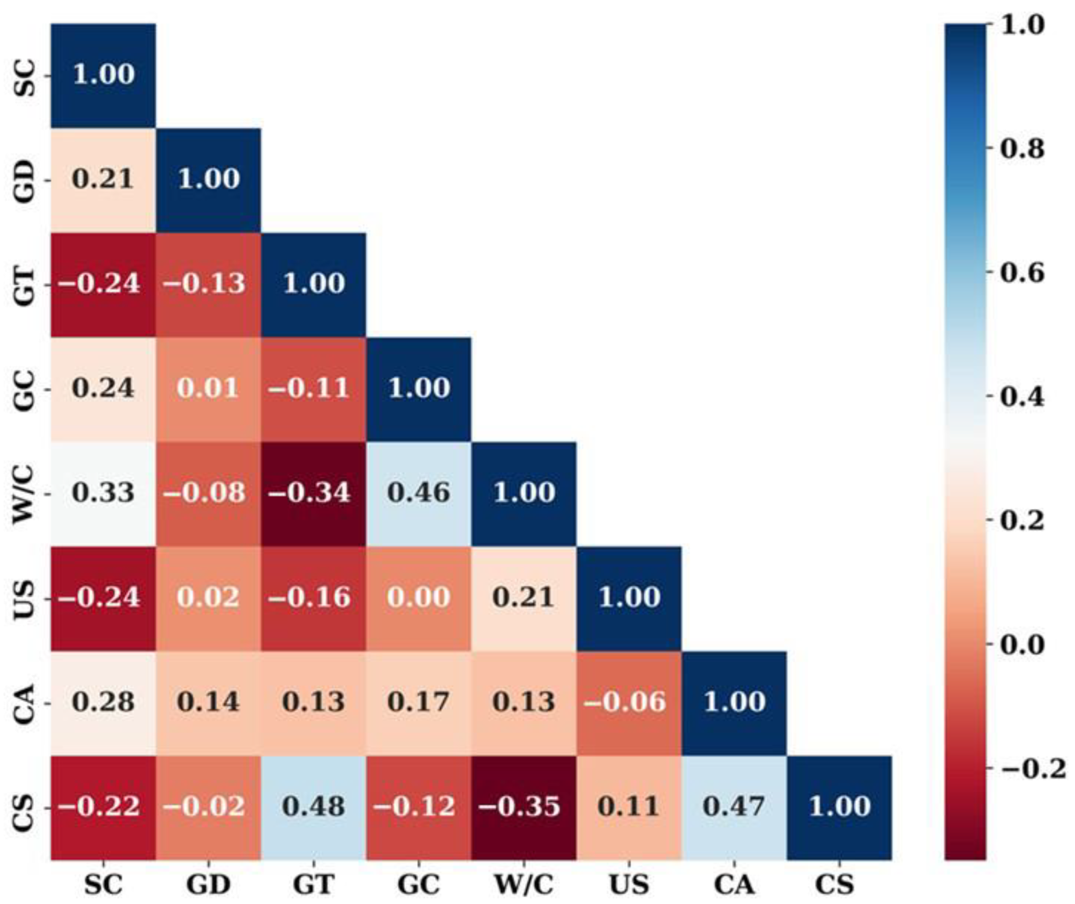
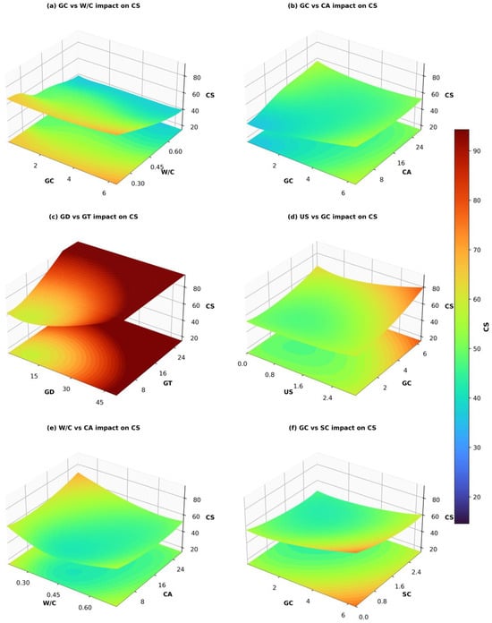
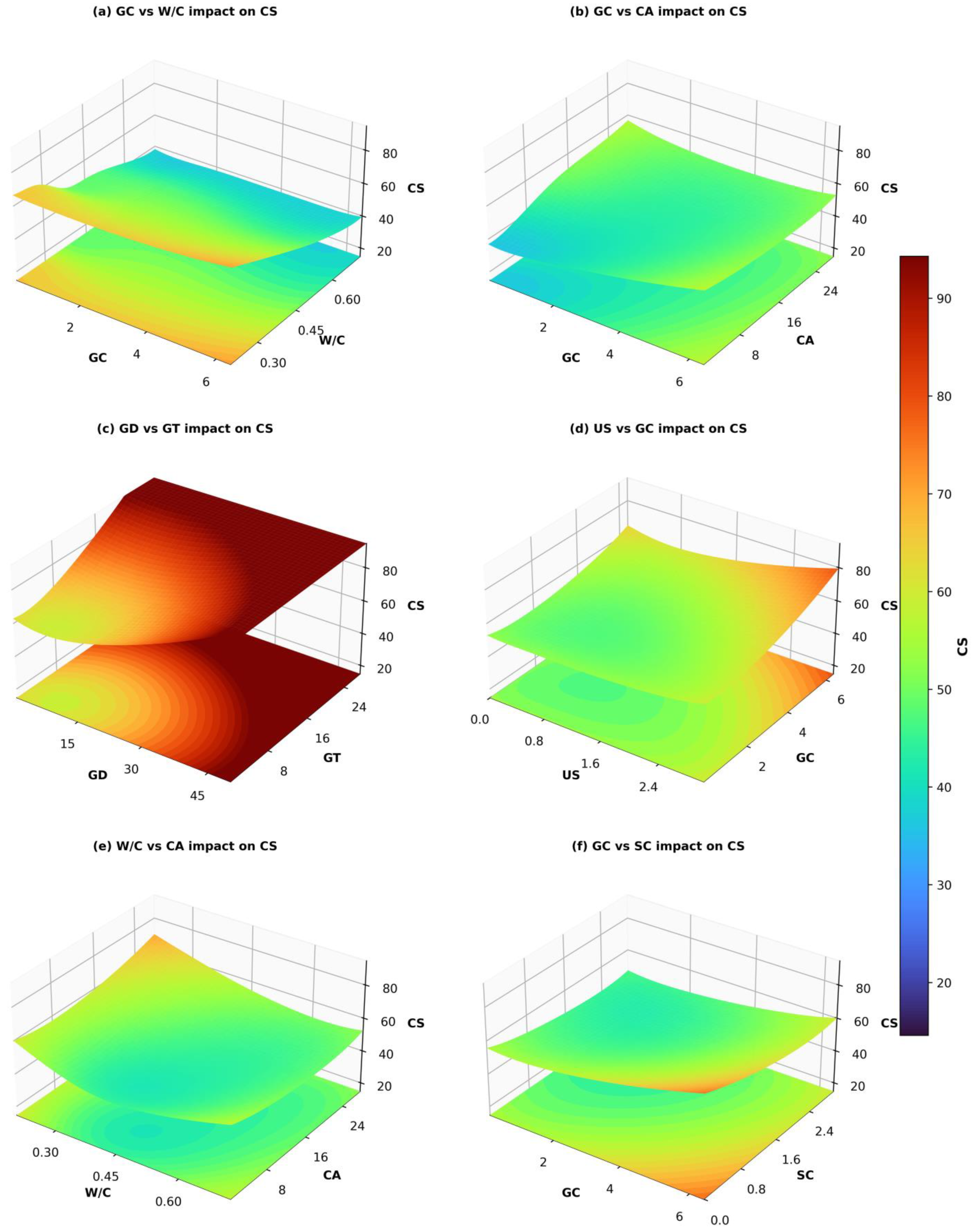
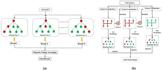
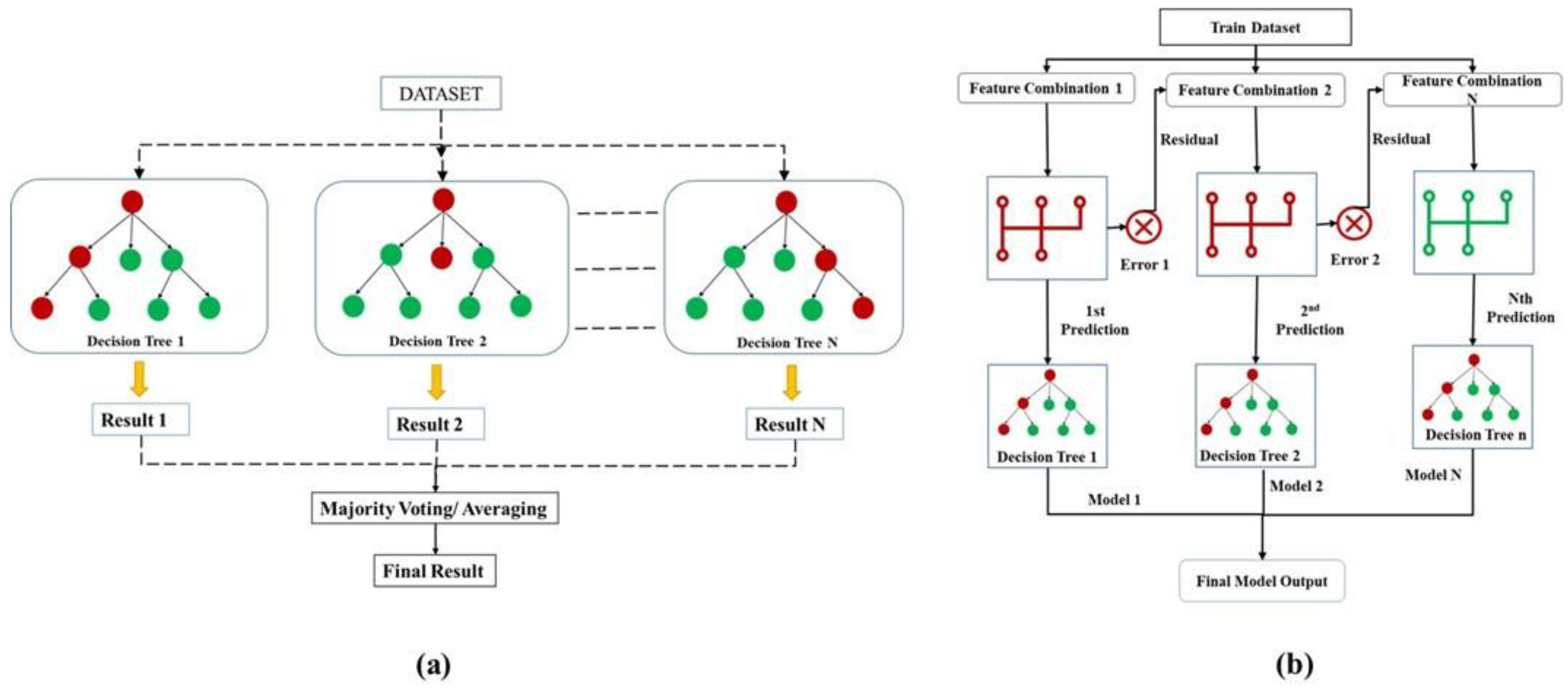
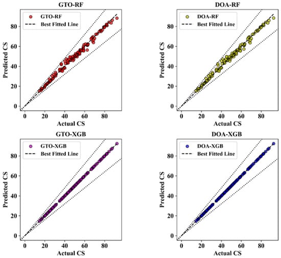
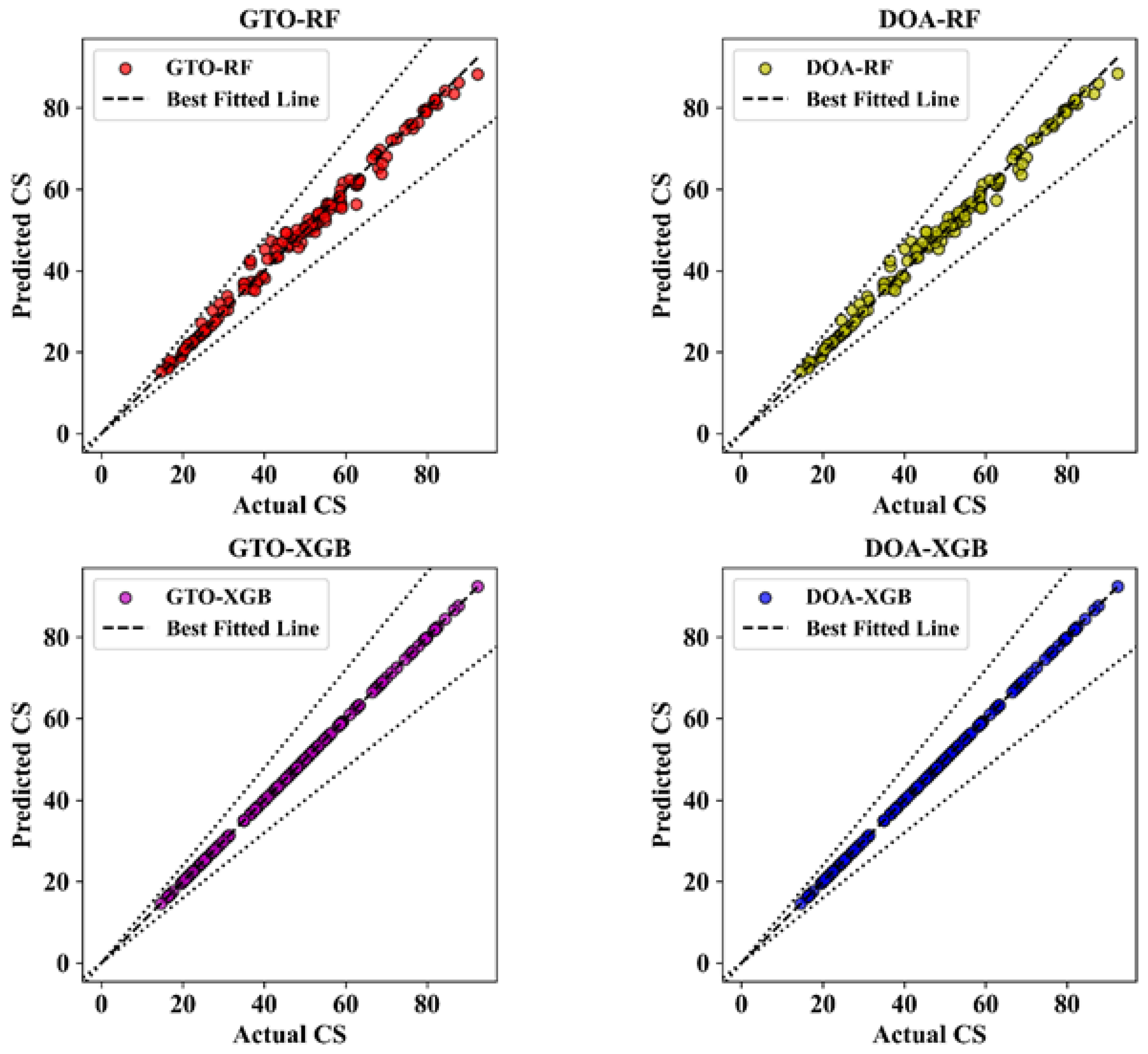
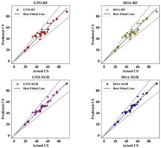
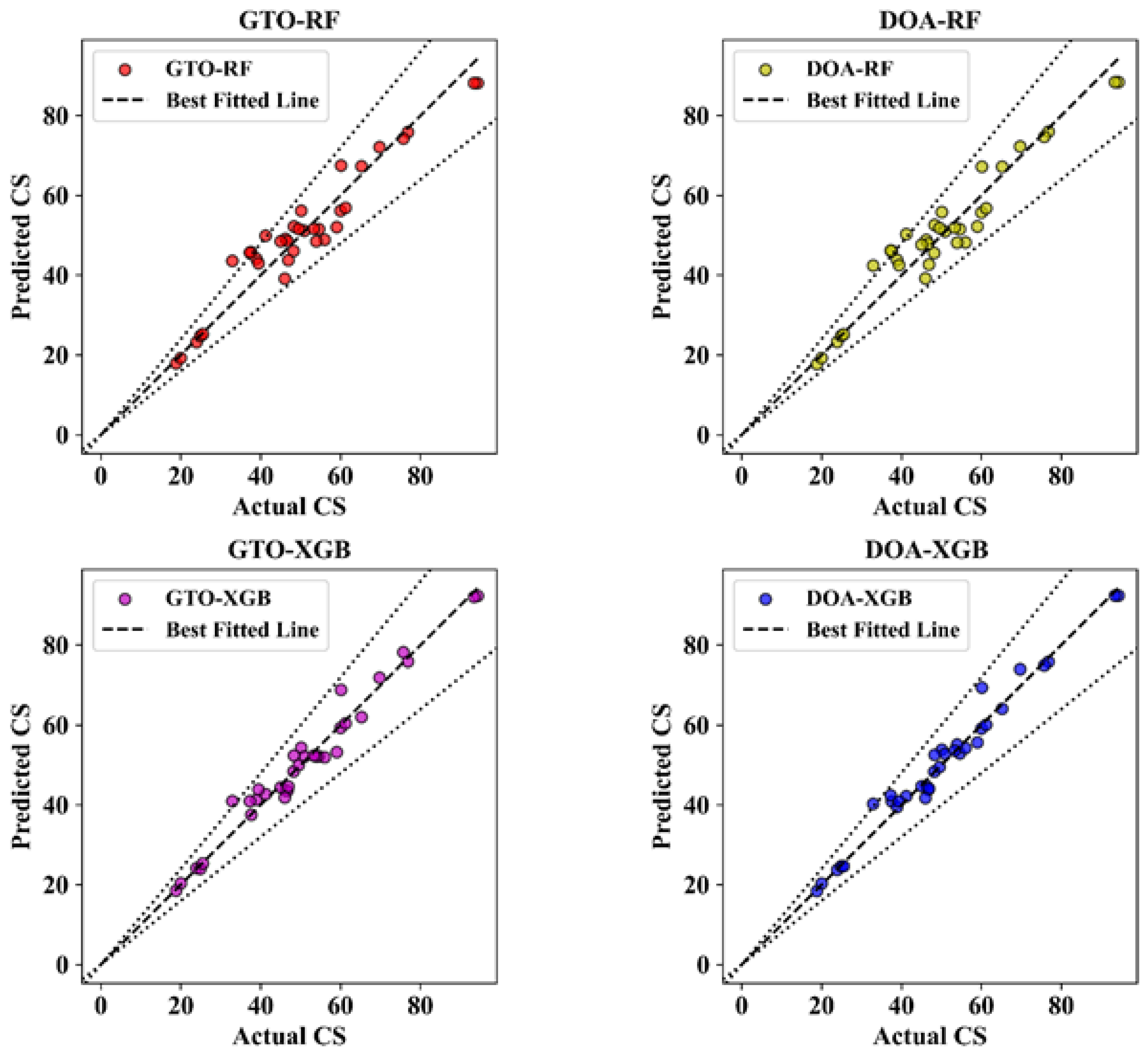
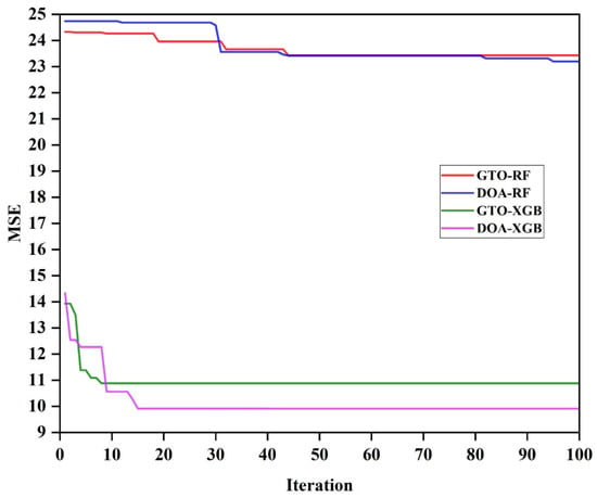
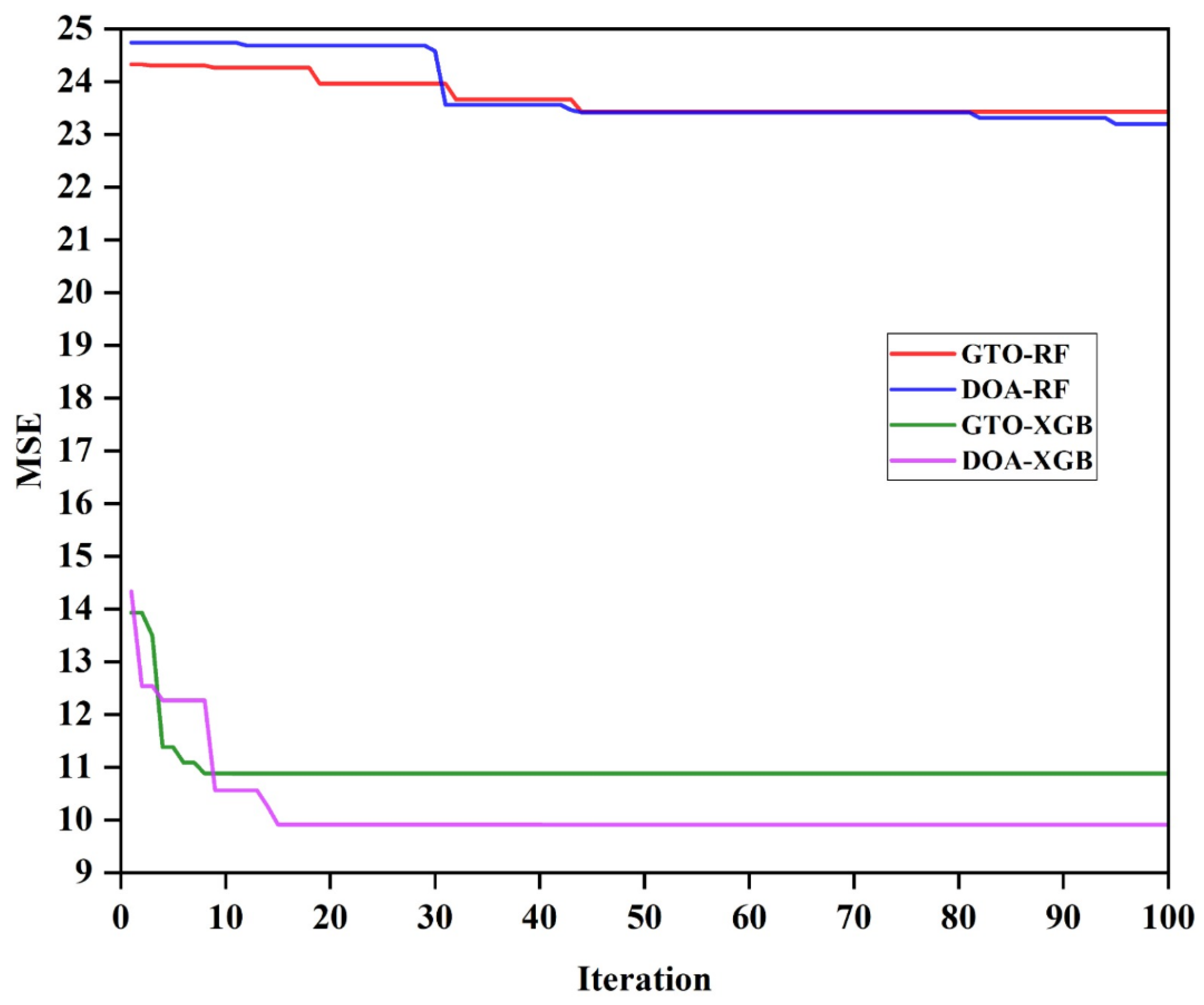
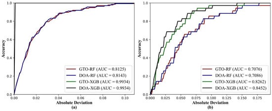
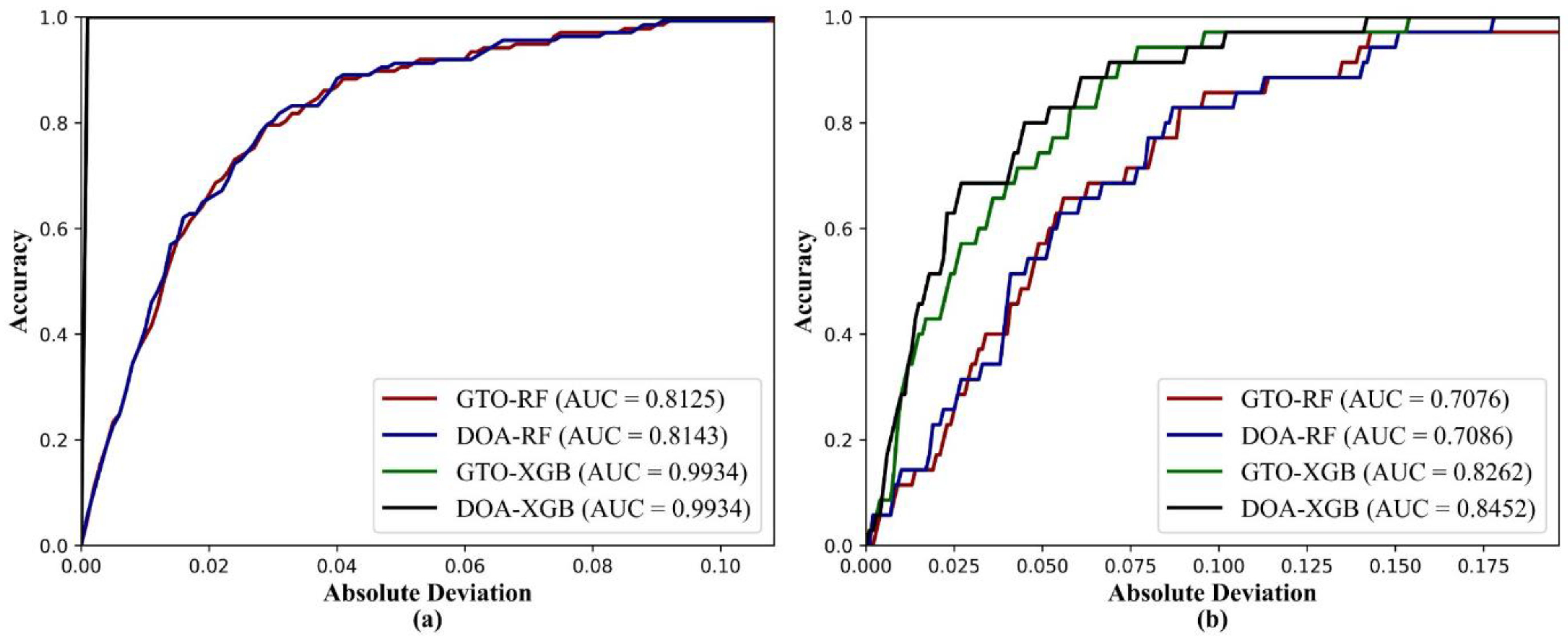
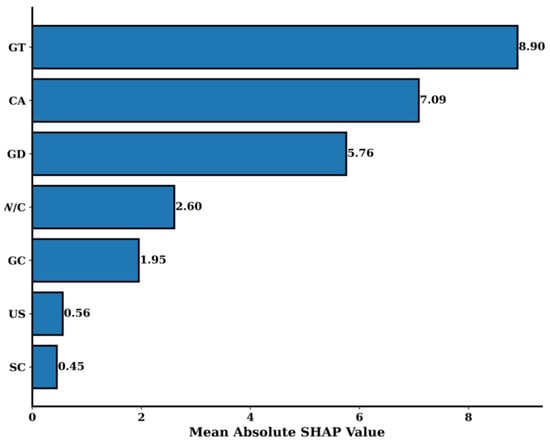
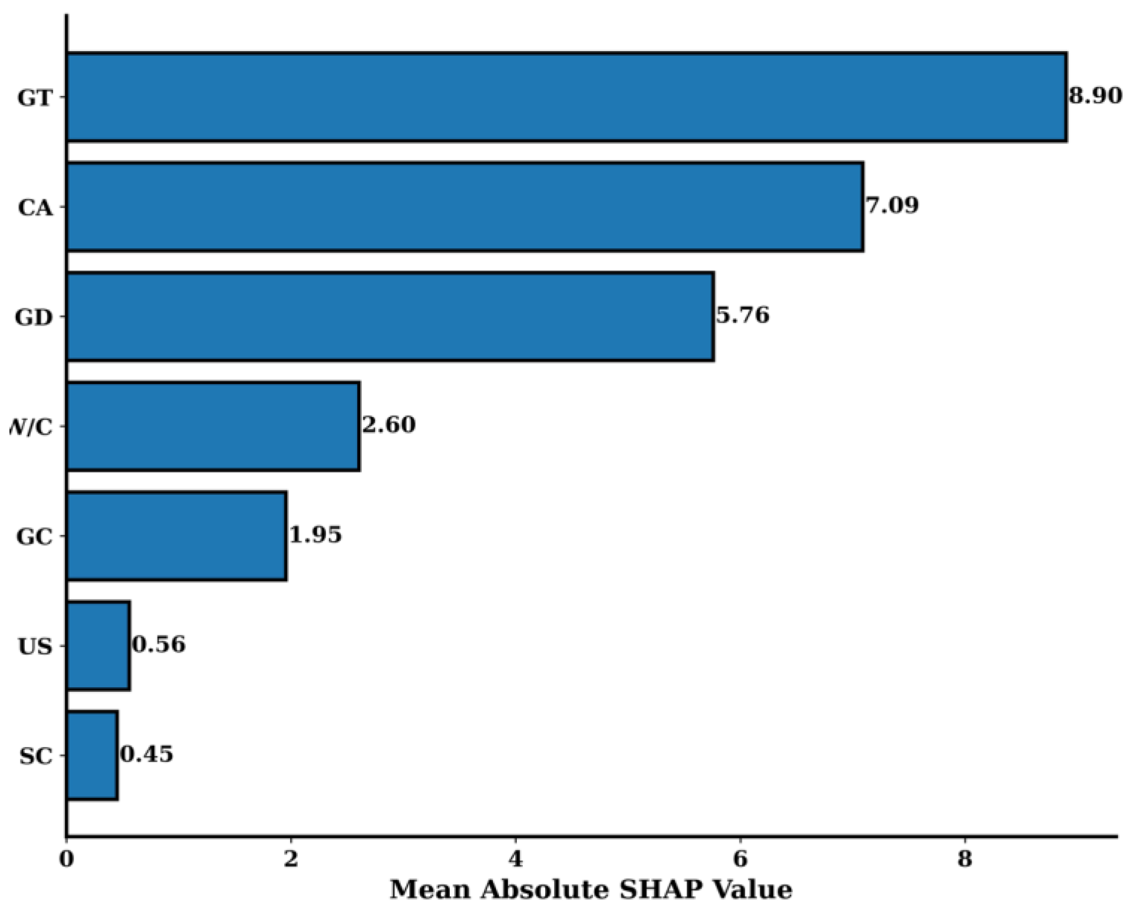
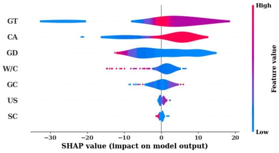
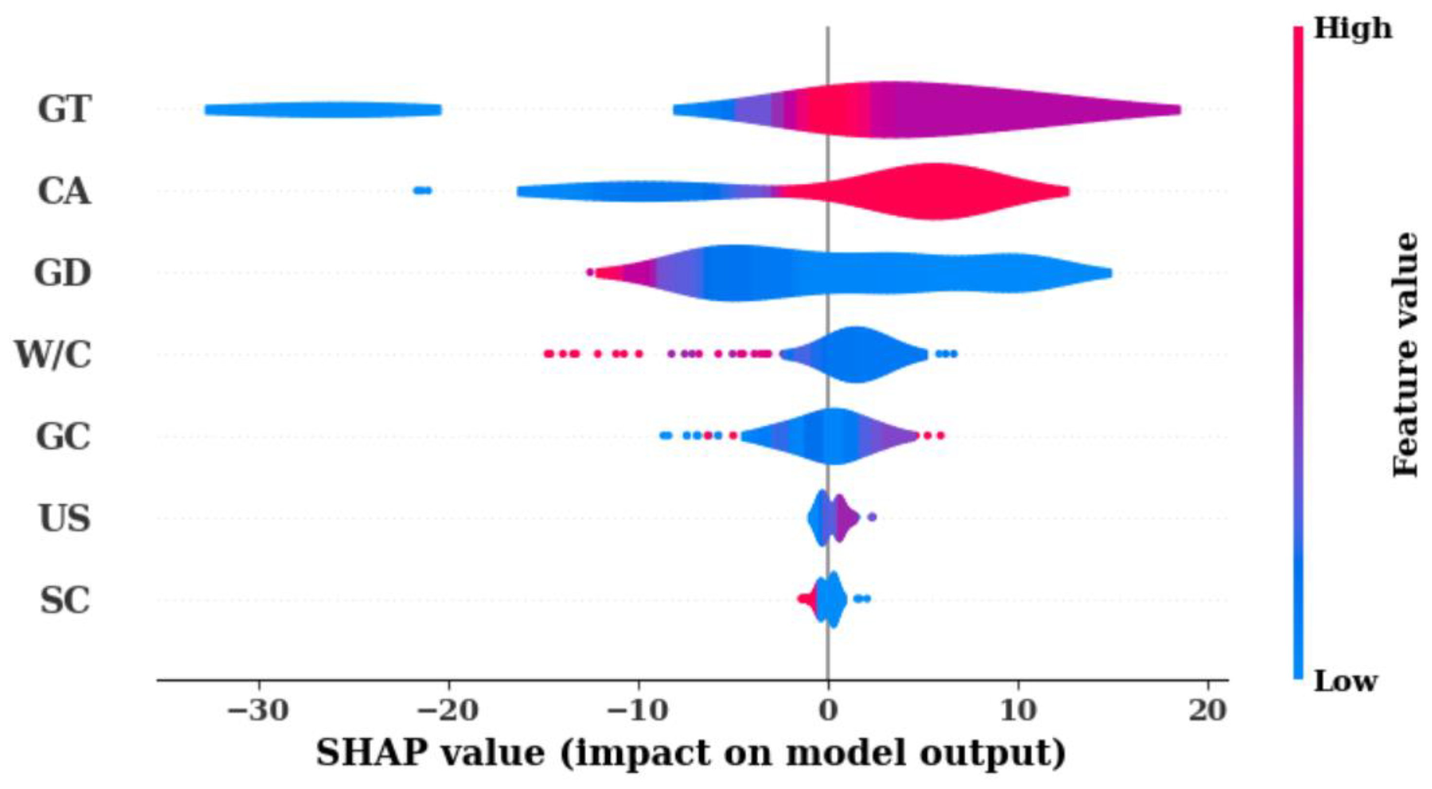


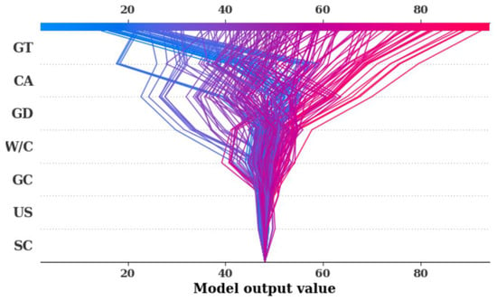
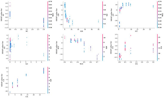
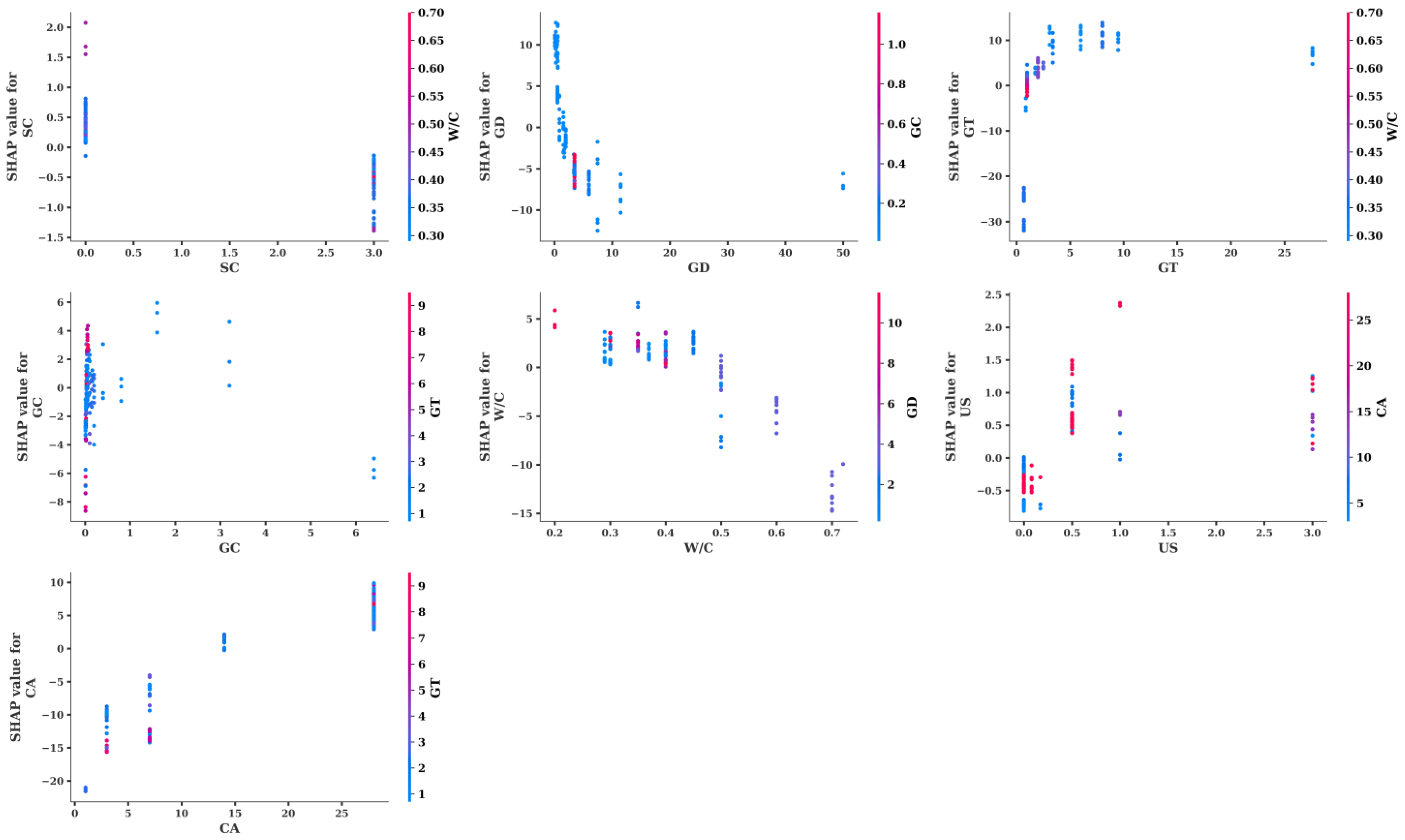
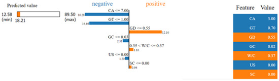
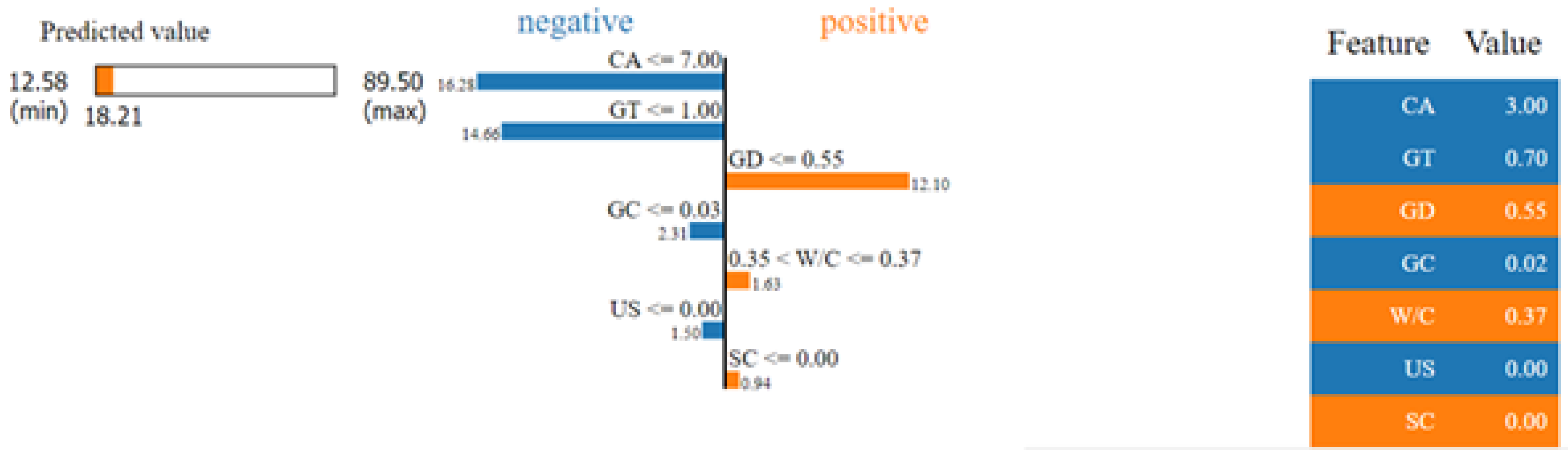
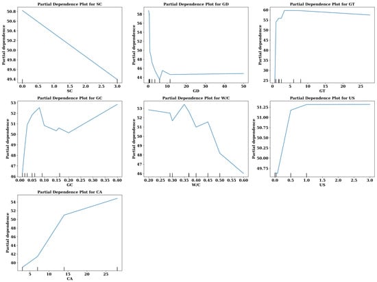
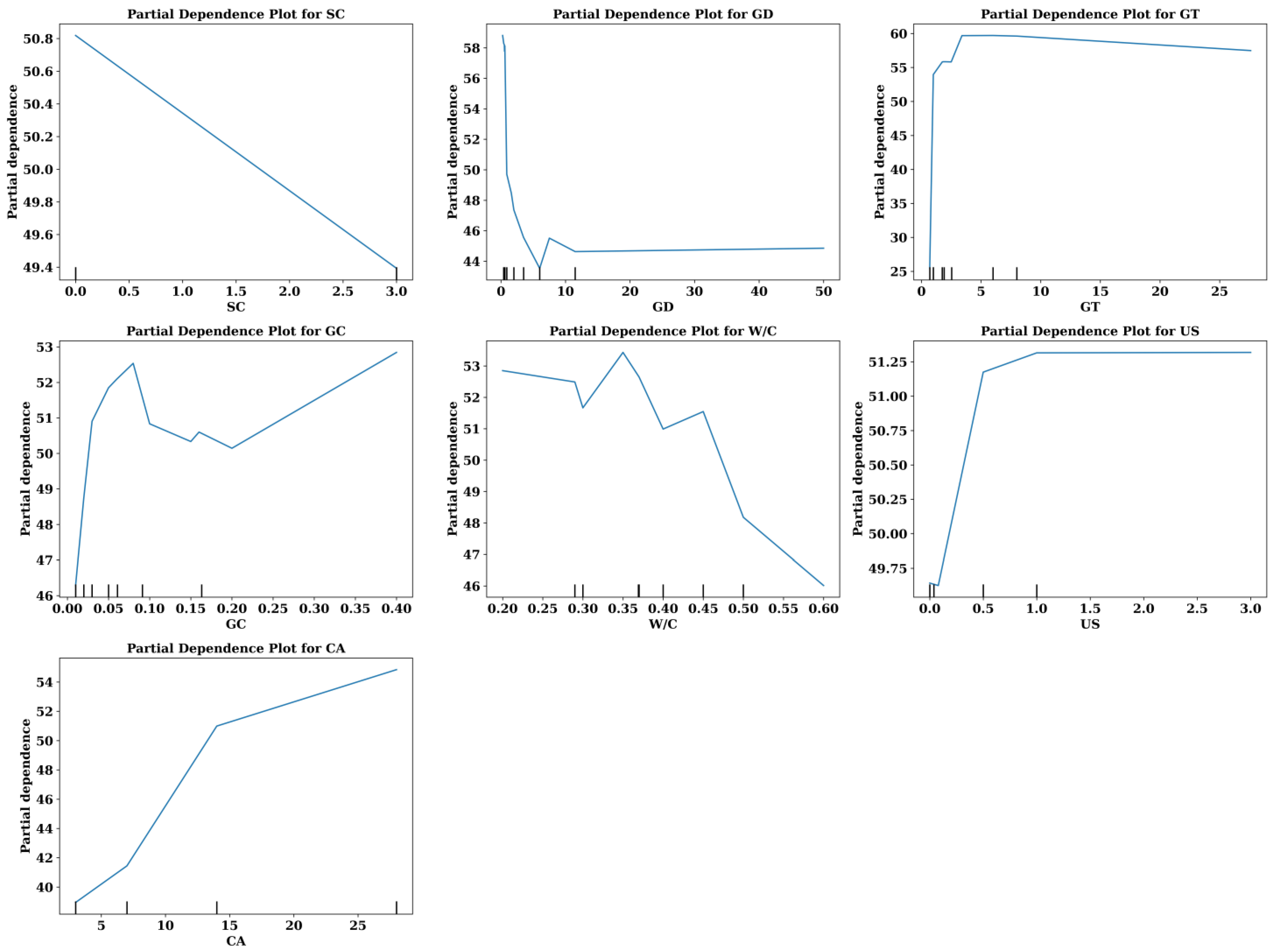
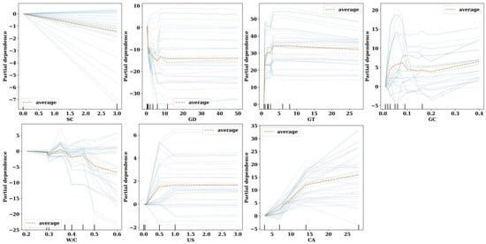
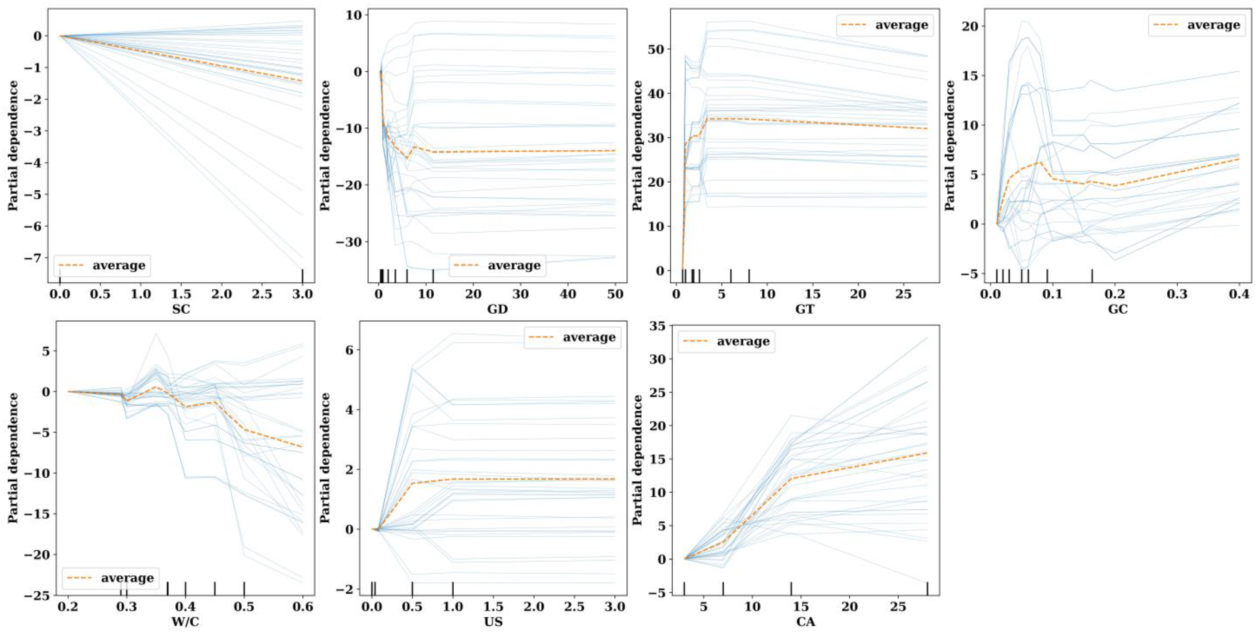
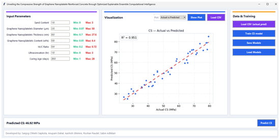
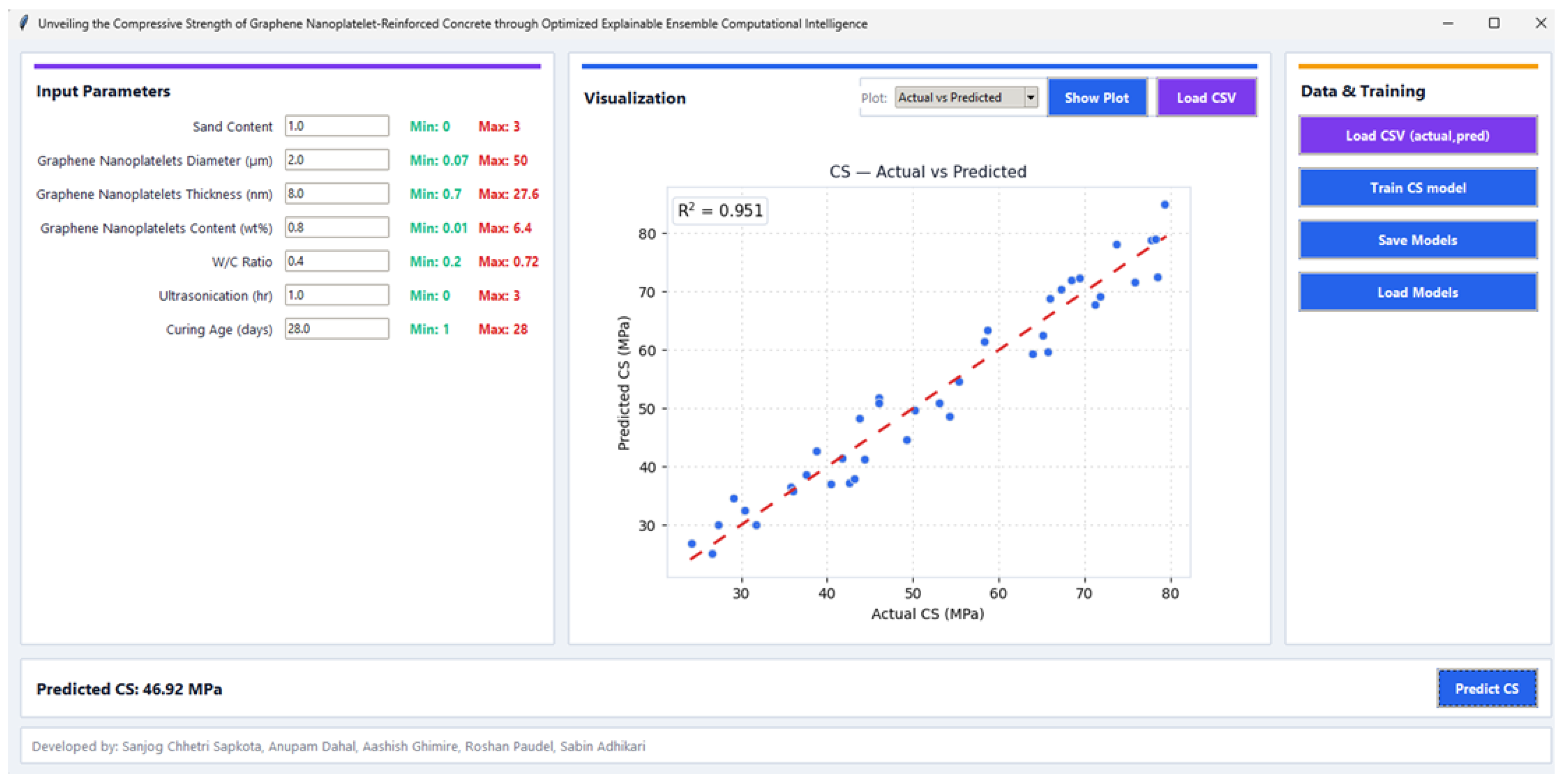

Disclaimer/Publisher’s Note: The statements, opinions and data contained in all publications are solely those of the individual author(s) and contributor(s) and not of MDPI and/or the editor(s). MDPI and/or the editor(s) disclaim responsibility for any injury to people or property resulting from any ideas, methods, instructions or products referred to in the content. |
© 2026 by the authors. Licensee MDPI, Basel, Switzerland. This article is an open access article distributed under the terms and conditions of the Creative Commons Attribution (CC BY) license.