


Abstract
Daily commuting in many peri-urban regions is dominated by private cars, causing congestion and greenhouse gas emissions. This research quantifies how a mixed public transport concept combining connector buses and organised ride-sharing can reduce road-traffic emissions in a regional rail corridor in southern Upper Austria. Commuter behavioural parameters and mobility patterns are informed by survey data collected from residents of the target region. Using land-use based sampling and k-means clustering, synthetic commuter populations and pickup points are generated, and ten configurations are simulated in four scenarios: car-only baseline, bus, ride-sharing, and combined mixed public transport (Mix-PT) using the microscopic traffic simulator TraffSim. Emissions are computed from the simulated vehicle trajectories with a physics-based fuel consumption model. Results show operational reductions of about 13% with buses, 18% with ride-sharing, and 28% in the Mix-PT scenario, relative to the baseline; all differences between the scenarios are statistically significant across the ten configurations. Car and ride-sharing trips remain time-competitive, while connector bus users accept longer journeys. Under the modelled acceptance constraints, combining feeder buses and ride-sharing can, therefore, contribute to lower commuting emissions in peri-urban rail corridors, although the size of the effect depends on the assumed behavioural parameters and service design and should be confirmed in field trials.
1. Introduction
Daily commuting in many metropolitan and peri-urban regions is still dominated by motorised private transport [1]. In the morning and evening peaks, high car use leads to recurrent congestion, long and unreliable travel times, and substantial greenhouse gas (GHG) emissions [2]. In areas with low-density settlements or limited public transport, the private car is often the only competitive option, even where rail corridors exist, because the stations are difficult to reach without a car.
Research on public transport has accordingly shifted from the planning of fixed-route, fixed-schedule networks towards more flexible and integrated service concepts. Flexible and demand-responsive transport (DRT) services were first discussed as a means to serve low-density areas and specific user groups at acceptable cost [3]; with the emergence of shared mobility, such services are increasingly seen as feeders that close the first and last mile to high-capacity lines [4]. DRT and connector bus services have been studied as feeders to rail and bus rapid transit (BRT) corridors, with evidence that they reduce car use and emissions when designed around existing fixed-schedule services [5,6], while agent-based evaluations also highlight that flexible services in low-density areas require careful dimensioning to avoid excessive vehicle mileage [7,8]. In parallel, ride-sharing has been investigated both as a stand-alone mode and in combination with public transit, where integrated matching of rides to transit stations can substantially increase the number of served trips [9]. The willingness to share rides depends on a range of socio-demographic, economic and attitudinal factors [10], and individual acceptance thresholds and departure flexibility dominate the achievable pooling rates and modal shift [11,12]; pooling can substantially reduce vehicle kilometres and road-traffic emissions compared to single-occupancy travel [13]. More recently, multi-mode public transit networks are increasingly assessed from a sustainability perspective, including their resilience to disruptions [14], and within land-use and transport models for climate change mitigation [15].
Agent-based simulation has become the standard tool for evaluating such multimodal and on-demand concepts at the level of individual travellers [8,16]. Large-scale frameworks such as MATSim [17] and FleetPy [18] have been used to assess ride-pooling, DRT and shared mobility services [8,19,20], and SimMobility couples activity-based demand with a microscopic short-term simulator [21,22]. Optimisation-oriented studies address the control of shared fleets [23]. Most of these studies focus on city-scale demand, and several of the platforms represent road traffic by queue-based flow models or precomputed network travel times, so that the effect of the services on congestion and driving dynamics is captured only approximately. Microscopic traffic simulators such as SUMO [24], in turn, reproduce vehicle dynamics in detail but do not natively provide the commuter-level decision logic required to model mode fallbacks between bus, ride-sharing and car. Synthetic population methods that incorporate land-use attributes are key to translating behavioural heterogeneity into such agent-based demand models [25].
Despite this body of work, there is limited quantitative evidence on how combined “mixed public transport” (Mix-PT) concepts, which integrate connector buses and organised ride-sharing as feeders to a regional railway, perform at the system level in a peri-urban corridor under survey-based behavioural constraints, and how they compare with car-only commuting. The contribution of this study is threefold and should be distinguished accordingly:
- Contextual novelty: connector minibuses and organised ride-sharing are evaluated separately and in combination as feeders to an existing regional rail line in a peri-urban corridor in Upper Austria, based on a synthetic commuter population derived from a regional survey on commuting behaviour and on the acceptance of both services.
- Modelling contribution: the study integrates, within one microscopic simulation, a commuter state automaton with survey-based mode priorities and individual acceptance thresholds, pre-trip and online planning of bus routes (LVNS optimisation with dynamic insertion) and ride-sharing matches, microscopic vehicle dynamics at junctions and in queues, and trajectory-based fuel and estimation. In contrast to the platforms above, TraffSim [26] thereby links individual mode decisions and the resulting vehicle movements directly to congestion and emission effects on the road network. The individual methods are established; the contribution lies in their integration and application, not in new algorithms.
- Policy contribution: the combined and individual effects of both services are quantified with paired comparisons across ten commuter configurations, together with service indicators relevant for dimensioning, such as bus loads and mileage, the share of eligible drivers without a matched rider and the share of car-less commuters left unserved.
The hypothesis is that combining both services achieves greater reductions than either service alone, while keeping door-to-door travel times broadly competitive with car use. Four scenarios are simulated for each of ten independently sampled commuter configurations: a car-only baseline, a bus scenario with new connector bus lines, a ride-sharing scenario, and a combined Mix-PT scenario. Across scenarios, emissions, travel times, mode choices and the utilisation of connector buses and ride-sharing are compared, addressing both aggregate system effects and distributional aspects such as achievable pooling levels and the share of commuters that can be served under the given acceptance thresholds.
The results confirm the hypothesis: the Mix-PT scenario reduces road-traffic emissions by approximately 28% relative to the car-only baseline, significantly more than connector buses alone (13%) or ride-sharing alone (18%), although less than the sum of both, while door-to-door travel times for car and ride-sharing users remain broadly comparable to the baseline, and connector bus users accept moderately longer journeys.
2. Materials and Methods
The approach is based on a microscopic, scenario-driven commuter simulation that enables quantification of the effects of introducing and combining feeder bus and ride-sharing services in a realistic regional context. The simulation is implemented in TraffSim [26], a microscopic, time-discrete traffic simulation framework developed at FH Upper Austria, implemented in Java. The road network is imported from OpenStreetMap and represented as a graph of lane and road segments. A dedicated Mobility as a Service (MaaS) module supports multi-modal commuter traffic: each commuter travels from their home location to a destination train station using a prioritised list of transport modes (single car, ride-sharing as driver or passenger, and connector bus combined with train). Static bus routes are optimised using an LVNS metaheuristic, dynamic pickup requests are handled by an online insertion algorithm, and ride-sharing routes are computed by a time-slot-based greedy search; the algorithms are described in detail in Section 2.7. For a fixed morning peak demand, several mobility scenarios are compared that differ in the availability of feeder buses and ride-sharing. Each scenario is evaluated with respect to emissions, travel times, and the utilisation of the newly introduced services.
2.1. Study Region and Commuting Demand
The model region is a commuter corridor in southern Upper Austria connecting several municipalities and railway stations along the line towards Linz, as shown in Figure 1. The region is characterised by a mix of small towns with direct rail access and surrounding settlements with limited public transport provision. Commuters from the surrounding settlements who travel along the rail corridor predominantly use the private car, as rail access requires a trip to one of the stations.
Figure 1.
Simulated road network of the model region (grey lines), the rail link to Linz (dashed grey lines) and the connector train stations (train symbols).
Background traffic is generated from the origin–destination (OD) matrix of car drivers of the Upper Austrian traffic survey 2012 [27]. The matrix contains the car trips between all pairs of municipalities, expanded to the resident population and resolved by the hour of trip start, and, thus, captures the temporal variation of travel demand throughout the day. For each OD relation, the route through the road network was determined, and all relations whose route passes through, originates from or terminates within the simulated network were retained. For these relations, background vehicles were scheduled according to the hourly trip counts of the matrix and follow their route through the simulated network, so that both local and through traffic are represented. The background traffic is identical in all scenarios and configurations; a simulation run containing only the background traffic serves as the reference for the emission accounting (Section 2.6).
The demand model represents individual commuters with home and work locations in the region. Each commuter record in the configuration file contains the following attributes:
- Spatial attributes: home location (longitude, latitude), workplace location, source train station (nearest boarding point on the rail corridor), and destination train station.
- Temporal attributes: request time (simulation start for requests known in advance, later for requests appearing during the simulation) and the targeted train connection.
- Mode availability: a flag indicating whether the commuter owns a car, and a flag indicating whether they are eligible to act as a ride-sharing driver.
- Transport priorities: an ordered list of preferred transport modes (e.g., ride-sharing > bus > car), used by the state automaton to select among feasible alternatives.
- Acceptance parameters: maximum acceptable walking distance to a pickup point or station, waiting timeout (maximum time a commuter waits for a ride-share or bus before falling back to the next priority), and a bus-to-car travel time acceptance factor , which defines how much longer a bus journey may be relative to the equivalent car trip [11].
This information forms the input to the simulation and defines the trips to be realised in each scenario. The synthetic commuter population is derived from the STUDIA survey, a quantitative survey of commuters conducted within the SAMLA project together with a survey institute and promoted in the regional media. The survey was carried out via an online panel between 20 February and 8 March 2024; of 573 responses, 323 responses of work commuters could be evaluated. Its target group were work commuters (including apprentices) living in the municipalities Kirchdorf an der Krems, Micheldorf and Schlierbach at least 1 km from the nearest station, who commute at least four days per month by train, car or carpool to Linz or to a destination along the railway line. To obtain a representative sample, commuters from structurally similar small regions in Upper Austria commuting into the Linz area were surveyed as well; 11% of the respondents live in the district of Kirchdorf, the others in eight comparison districts (e.g., Urfahr-Umgebung 19%, Freistadt 13%, Perg 12%). The sample is balanced with respect to gender (52% male, 48% female) and covers all working age groups (18–29 years: 23%, 30–44 years: 33%, 45–64 years: 44%) and educational levels (compulsory school or apprenticeship: 41%, vocational middle school: 19%, upper secondary school: 19%, tertiary education: 21%). The questionnaire covered current commuting behaviour, personal attitudes, and the assessment of service attributes of the currently used mode and of the two alternatives micro public transport and ride-sharing, each rated on an acceptability scale from (entirely unacceptable) to (optimal) and by its importance. The resulting attribute importance ranks commuting time and punctuality far above all other attributes (followed by service frequency and fare), which motivates the representation of acceptance by travel-time based thresholds in the simulation (Table 1). For the spatial demand, the survey data were scaled up to the commuter population of the model region and aggregated to grid cells of 250 m × 250 m containing the number of commuters, their destination station and the train connection used. For the train connection considered here, the scaled data contain 193 commuters in 118 grid cells who board at one of the three source stations Micheldorf, Kirchdorf an der Krems and Schlierbach and continue along the line. Each commuter configuration is generated in four steps, combining the survey data with land-use information [25]:
Table 1.
Commuter and service parameters. TN denotes a normal distribution with mean and standard deviation truncated to . Realised values refer to all 1942 commuters of the ten configurations.
- 1.
- Home locations and request times. A total of 230 requests are drawn. For 90% of them (static requests, known at simulation start), a grid cell is drawn with a probability proportional to its number of commuters, and the home location is sampled within the cell from the CORINE Land Cover 2018 polygons [28], with land-cover classes weighted by their share of the population (e.g., discontinuous urban fabric 50%, continuous urban fabric 12%, complex cultivation patterns 11%). The remaining 10% (dynamic requests) appear during the simulation according to a Poisson process per source station until 10 min before the train departure, with station shares and locations sampled from the survey data of the respective station catchment. Requests within 500 m of their source station are removed, as these commuters are assumed to walk to the station. The resulting configurations contain between 176 and 206 commuters (mean 194), which corresponds to the scaled demand for this train connection.
- 2.
- Destinations. The destination station is drawn from the survey-based distribution of destination stations of the commuter’s municipality; the workplace is placed at a random bearing and a truncated-normally distributed distance from the destination station (Table 1).
- 3.
- Mode priorities and vehicle availability. Each commuter receives an ordered list of acceptable modes drawn from the categorical distribution given in Table 2. This distribution was derived from the STUDIA survey: the respondents’ current main mode and their stated likelihood of using a carpool and a micro public transport service were matched to the three modes car, ride-sharing and bus, and each respondent was assigned the ordered list of modes they would accept, ranked by the stated likelihood of choosing them (e.g., “prefer carpooling, would also use micro public transport, otherwise drive” corresponds to ride-sharing > bus > car). The shares of these lists among the respondents define the category weights. Commuters whose list contains the car are car owners (95.5%); of these, a share of 50.4% is eligible to act as ride-share drivers.Table 2. Distribution of mode priority lists (realised shares over all ten configurations).
- 4.
- Acceptance parameters. Accepted walking distance, waiting timeout and the bus-to-car travel time acceptance factor are drawn independently from truncated normal distributions (Table 1), whose parameters were derived from the answers of the STUDIA survey. Consequently, the parameters are uncorrelated; the largest realised Spearman correlation between any two of them is .
To account for sampling variability, ten independent commuter configurations were generated with this procedure (1942 commuters in total). Since the grid data are already scaled to the commuter population, they are used as relative sampling weights without further expansion factors, and the number of requests is chosen such that the configurations reproduce the scaled demand for the considered train connection. Static requests are issued at simulation start (05:00), while the request times of the dynamic requests are spread almost uniformly between 05:00 and 06:45 (quartiles 05:28, 05:53 and 06:15).
The synthetic population reproduces the spatial structure of the scaled survey data closely. The shares of the three source stations Micheldorf, Kirchdorf an der Krems and Schlierbach amount to 29.4%, 42.7% and 27.9%, compared with 31.6%, 44.0% and 24.4% in the survey data. The destination stations are dominated by Linz Hauptbahnhof (27.7% simulated vs. 30.6% in the survey data), Kremsmünster (26.6% vs. 25.4%) and Nussbach (25.2% vs. 22.8%); over all eight destination stations, the total variation distance between the simulated and the survey distribution is 3.6 percentage points (3.5 for the source stations). On the level of the 118 survey grid cells, 92% of the cells are represented in the synthetic population, and the shares of commuters per cell correlate with the survey data (); the deviations result mainly from the small number of commuters per cell and from the removal of commuters living within 500 m of a station, who account for 17% of the scaled demand. Within a configuration, the commuters and all their attributes are identical across the four scenarios; only the priority list is reduced to the modes offered in the respective scenario (e.g., ride-sharing is removed in the bus scenario, and all commuters use the car in the car-only baseline).
2.2. Input Data and Scenario Generation
The simulation is driven by a set of input data sources that jointly define the commuter population, their behavioural parameters, and the available transport offer. First, the STUDIA survey and the acceptance parameters described above (Table 1) are translated into a commuter configuration. This configuration specifies, for each synthetic commuter, the home and work locations, request time, car availability and acceptance thresholds used by the state automaton.
In parallel, the infrastructure and service offer are described by a train schedule for the rail corridor and by a pickup point input file that defines the spatial locations at which commuters can board buses. The simulation considers a single train run of the regional S4 service in the morning peak, departing from Micheldorf at 06:51 and arriving at Linz Hauptbahnhof at 07:54; all commuters target this train, and all connector bus and ride-sharing trips are planned to meet its departure at the respective source station. Bus–train coordination is, therefore, modelled for one connection, and the effect of the service headway on waiting times is not considered. The pickup points were generated once and are identical in all configurations and scenarios. To obtain a compact yet well-covered set of access points for connector buses, spatial k-means clustering was applied to commuter home locations sampled from the land-use classes and population distribution of the region (as in step 1 above); the resulting cluster centroids define the pickup points, as shown in Figure 2. The number of clusters controls the density of pickup points and, thus, the walking distance to the nearest access point; k = 43 was selected by silhouette analysis [29] as the number of clusters with the highest average silhouette coefficient, i.e., the best separation of compact clusters of home locations. In the simulation, each pickup point is mapped onto the nearest road segment, where the bus stops on the side of the road that is closer along its route; whether the resulting location is a legal and safe boarding position is not checked. Combining the commuter configuration with the train schedule and pickup point data yields a commuter input file that serves as the complete demand-side input for the simulation.
Figure 2.
Home locations of the sampled commuters of one configuration (configuration 1), the 43 pickup points used in all simulations, and the three source train stations in the target region.
For each scenario (car-only baseline, bus, ride-sharing, Mix-PT), TraffSim [26] reads the commuter input file and the corresponding scenario-specific service definitions, executes the microscopic simulation, and produces simulation statistics. These statistics contain, among others, the realised mode choices, travel times, vehicle occupancies and emissions and form the basis for the analysis presented in Section 3.
2.3. Scenario Design
Four scenarios are defined that represent different configurations of the transport offer in the region:
- Car-only baseline: All commuters who own a car drive by private car from home to their destination station, without any feeder bus or organised ride-sharing offer; commuters without a car are not served.
- Bus scenario: New feeder bus services are introduced that connect residential areas without rail access to the three railway stations Micheldorf, Kirchdorf an der Krems and Schlierbach. Each bus operates a route that is optimised before the simulation (static route, Section 2.7); commuters who request a ride only during the simulation can additionally be inserted into this route (dynamic insertion). Commuters can choose these buses in addition to the private car and rail.
- Ride-sharing scenario: Commuters can act as ride-share drivers or passengers, forming pooled trips to railway stations or workplaces if acceptance constraints are satisfied.
- Mix-PT scenario: Feeder buses (static routes with dynamic insertion, as in the bus scenario) and ride-sharing are offered simultaneously, creating an integrated Mix-PT concept on top of the existing rail and road network.
For each of the ten commuter configurations, the full set of four scenarios (car-only baseline, bus, ride-sharing, Mix-PT) is simulated, resulting in 40 simulation runs in total. Within a given configuration, the underlying commuter demand (origins, destinations, request times and acceptance parameters) is identical across scenarios, so that differences in outcomes can be attributed solely to the changed transport offer and the resulting mode and route choices.
2.4. Simulation Model and Implementation
The core of the TraffSim [26] MaaS module is a commuter state automaton. Each commuter is represented as an agent that transitions between discrete states during the simulation horizon, as shown in Figure 3. The states cover (i) planning and candidate states for bus and ride-sharing services, (ii) accepted and in-vehicle states for bus, train and ride-sharing, (iii) car usage as single driver or ride-share driver, and (iv) terminal states for successfully completed trips and failures to reach the destination. Transitions between states are controlled by the transport offer of the respective scenario and by commuter-specific acceptance parameters (maximum detour, walking distance, latest acceptable arrival time, occupancy limits).
Figure 3.
Possible transitions in the commuter state machine.
The road network and regional rail lines are represented as a unified multi-modal network. For each of the four scenarios (car-only baseline, bus, ride-sharing, Mix-PT), the simulation proceeds as follows:
- 1.
- Initialisation: All commuters enter the SCHEDULED state. The road network, rail timetables, and connector bus routes for the given scenario are loaded. Commuters with potential_ridesharing_driver = true and a private car (owns_a_car = true) are registered as candidate ride-share drivers.
- 2.
- Pre-simulation routing: One static connector bus route per source station is computed once before the simulation starts via the LVNS metaheuristic. Commuters whose requests become known only during the simulation (about 10% of all commuters) can later be inserted into these routes by the dynamic insertion algorithm. Ride-share driver routes are assembled by the time-slot-based greedy search (Section 2.7), grouping drivers with compatible riders based on shared destination station.
- 3.
- Mode assignment: Each commuter evaluates feasible modes in the order specified by transport_method_priorities. A mode is accepted if the projected door-to-door travel time does not exceed the personalised threshold derived from car_bus_travel_time_factor and the individual car travel time. Commuters without a private car who cannot be matched to any bus or ride-share service transition to UNABLE_TO_REACH_DESTINATION.
- 4.
- Time-discrete simulation: Vehicles and commuters advance through the simulation in discrete time steps of ms. The simulator tracks each commuter’s state sequence, waiting at pickup points, boarding a connector bus, transferring to the regional train, or travelling by private or shared car, and records the resulting waiting times, in-vehicle times, and transfer events.
- 5.
- Output logging: On trip completion, the simulator records the realised mode, total travel time, instantaneous vehicle occupancy, and the final state (RIDE_DONE or UNABLE_TO_REACH_DESTINATION). Fuel consumption and emissions are accumulated for every vehicle in every time step from its simulated trajectory (Section 2.6).
This simulation procedure yields the per-trip and per-vehicle data needed to compare the four scenarios across all ten commuter configurations: commuter-attributable road-traffic emissions, travel-time distributions by realised mode, modal split, connector bus and ride-share vehicle occupancies, and the share of commuters whose stated transport priorities could be satisfied.
2.5. Traffic Flow, Junction and Queue Representation
Road capacity, queuing and spillback are not prescribed by explicit capacity values but emerge from the microscopic interaction of vehicles. The road network is generated from OpenStreetMap data and represented at lane level; the number of lanes, speed limits, turn restrictions and one-way regulations are taken from the OpenStreetMap attributes. The longitudinal motion of every vehicle is governed by the Intelligent Driver Model (IDM) [30], which determines the acceleration from the vehicle’s speed, the gap and the speed difference to the vehicle ahead (desired time gap 1.5 s, minimum gap 2 m, maximum acceleration 1., comfortable deceleration ), and lane changes follow the MOBIL model [31]. Junctions are modelled as separate entities with lane-to-lane connectors [32,33]: in every time step, each junction decides which approaching vehicles may enter, giving precedence to traffic signals, then to road signs and otherwise applying the right-before-left rule; roundabouts are supported as well. Entry permissions are re-evaluated continuously and can be revoked, e.g., when the exit lane is blocked. As a consequence, vehicles queue upstream of a junction when it cannot be entered, and queues propagate backwards into upstream road segments and junctions when their storage space is exhausted, so that spillback is reproduced by the car-following dynamics. The time step of t = 100 ms is small compared with the IDM time gap and the typical vehicle headways, so that the discrete update does not limit the resolution of queue formation and dissipation.
2.6. Fuel Consumption and Emission Model
Emissions are not derived from fixed per-kilometre emission factors but from the simulated vehicle trajectories. TraffSim applies the physics-based fuel consumption model of Treiber et al. [34,35] to every vehicle in every simulation time step, using its instantaneous speed v, acceleration a and the slope of the current road segment. The mechanical driving force is
and the required engine power is , where is the base power of auxiliary consumers. The fuel flow follows from an engine consumption map that relates engine speed and torque to specific fuel consumption, including engine friction losses; in each time step the gear that minimises the fuel flow is selected, and at standstill the engine consumes its idle rate. The model parameters correspond to a typical mid-size gasoline passenger car [34,35]: vehicle mass kg, rolling resistance coefficients and s/m, drag coefficient , frontal area , air density , base power kW, dynamic tyre radius m, maximum engine power 110 kW, displacement 1.8 L, minimum specific fuel consumption 185 g/kWh, idle consumption 0.8 L/h and five gears with overall transmission ratios 16.4, 13.9, 7.8, 5.26 and 3.79. All vehicles are modelled as gasoline vehicles, and is obtained with a tank-to-wheel conversion factor of kg per litre of fuel. This value lies at the upper end of published factors for gasoline (e.g., 2.32 kg/L according to [36]); since the same factor applies to all vehicles, it scales the absolute emissions by about 3% but does not affect the relative differences between the scenarios. The connector buses are small 20-seat minibuses; in the simulation they differ from passenger cars only in vehicle length and use the same consumption parameters, so that their fuel consumption is likely underestimated (see Section 3.6). Stop-and-go driving, idling in queues, detours and congestion, therefore, enter the emission estimate directly through the simulated trajectories.
The emissions of a simulation run r are summed over all vehicles i and time steps t. To isolate the emissions caused by commuter traffic, the emissions of a reference run containing only the background traffic are subtracted:
, thus, contains the direct emissions of all commuter vehicles (private cars, ride-share vehicles and connector buses) together with the change in emissions of the background traffic caused by the commuters, e.g., through additional or relieved congestion. Commuters without a private car who cannot be served by a bus or a ride-share vehicle end in the state UNABLE_TO_REACH_DESTINATION; no vehicle departs for them, so they cause no emissions. For consistency, commuters without a car are also not counted as car drivers in the car-only baseline: since per-vehicle emissions are not recorded separately, the baseline emissions of each configuration are reduced by the car-less commuters’ share of the total predicted car drive time (2–7% depending on the configuration), neglecting the small effect of these vehicles on the congestion of the background traffic.
Emissions are computed per vehicle rather than per passenger: a ride-share vehicle emits according to its own trajectory, and passengers influence emissions only through the detours required to collect them. Per-passenger values are obtained by dividing the average emissions per vehicle-km by the average occupancy of each mode.
The system boundary is operational (tank-to-wheel) road-traffic within the simulated network during the morning peak. Connector buses start at the train station, collect their passengers and return to the station, where they end their service; the approach from the station to the first pickup point is, therefore, counted as empty running. Bus departures to which no commuter is assigned are not operated and cause no emissions. Emissions of the regional train are not included, as the train operates according to the same timetable in all scenarios. Upstream (well-to-tank) emissions of fuel supply, vehicle production, cold-start excess emissions and pollutants are outside the scope of this study.
2.7. Routing Algorithms
2.7.1. Rideshare Routing Algorithm
The rideshare routing algorithm employs a time-slot-based greedy search strategy to construct pickup routes for rideshare drivers. It operates on a per-driver basis and plans the complete pickup route of a driver before the driver departs. Drivers are processed sequentially in the order in which they appear in the simulation: drivers known at simulation start are routed in the first time step in the order of the commuter input file, which results from the random sampling of the population, while drivers whose requests appear later are routed shortly before their latest departure time. In both cases, only riders who have not yet been assigned to another driver can be considered, and among these the driver selects the one requiring the smallest detour first. This first-come, first-served procedure reflects the operation of a ride-sharing platform in which requests are handled as they arrive, rather than a global assignment that would require all requests of all drivers to be known in advance.
As a prerequisite, each commuter is assigned a latest departure time, the latest point in time at which they must leave their home location in order to reach the destination train station no later than the scheduled train arrival time. For rideshare drivers, this departure window is extended by a driver margin of 5 min, allowing them to depart slightly earlier than necessary to accommodate detours for passenger pickup.
The routing procedure for a given rideshare driver begins at their current road position. A random upper bound on the number of passengers to collect is drawn uniformly from the integers , where is the number of seats of the vehicle including the driver’s seat. The upper bound can, therefore, reach the full passenger capacity of three; drawing it randomly represents the heterogeneous willingness of drivers to carry several passengers. The algorithm then enters an iterative greedy selection loop that repeats until either this passenger limit is reached or no further eligible riders can be found.
In each iteration, the algorithm identifies the set of candidate riders: commuters who are in the POTENTIAL_RIDESHARING_RIDER state, share the same destination train station as the driver, and have not yet been assigned to this driver. For each candidate, two route costs are computed using the double-sided routing utility: (1) the cost to travel from the driver’s current position to the candidate’s nearest road position (the pickup cost), and (2) the cost to continue from the candidate’s location to the destination train station. Both computations draw on historical drive-time data indexed by the hour of the train’s arrival.
A candidate is considered eligible only if all of the following temporal constraints are satisfied. First, the estimated arrival time at the rider’s location, derived from the driver’s current departure time and the pickup cost, must fall within the rider’s acceptable waiting window, which is defined as the period between the start of the rider’s waiting timeout and their latest departure time (or, in the case of a rider who is also a potential driver, within the driver margin beyond the latest departure time). Second, the projected arrival time at the train station, combining the pickup cost and the cost of the subsequent leg to the station, must not exceed the scheduled train arrival time.
Among all eligible candidates, the one with the minimum pickup cost is selected greedily. The corresponding pickup route segment is appended to the accumulated route, removing the last road segment of the pickup sub-route to avoid duplication at the join point. The driver’s current position is then advanced to the selected rider’s road position, taking into account which side of the road (primary or opposite segment) is geometrically closer, and the rider’s state is tentatively recorded. If the pickup route spans only a single road segment and at least one rider has already been collected, the newly selected rider is inserted into the pickup list in positional order along that segment, rather than appended to the end, to preserve route consistency.
After the loop terminates, the algorithm computes a final route leg from the last pickup position to the train station stop. If this leg is successfully found, all collected riders have their states transitioned to ACCEPTED_RIDESHARING_RIDER, and a complete Route object is returned comprising all accumulated road segment IDs. If no riders were collected, or if the final leg to the train station cannot be computed, the algorithm returns null and clears any tentatively assigned riders from the driver’s pickup list.
The overall complexity of the algorithm is , where is the maximum number of passengers, n is the number of potential riders, and R is the cost of a single routing query. Since is bounded by the small vehicle seat count, the approach remains computationally tractable even for large commuter populations.
2.7.2. Static Bus Route Algorithm
The static bus route algorithm determines, for each of the three source stations, the route of one connector bus that maximises the number of commuters transported to this train station. It combines a greedy initialisation phase with a Large Variable Neighbourhood Search (LVNS) metaheuristic to iteratively refine the route.
The service structure is fixed, while the route within it is optimised. Fixed inputs are: one bus with 20 seats per source station; the route starts and ends at the train station; the candidate pickup points (Section 2.2); the assignment of each potential bus user to the nearest pickup point within their accepted walking distance; and the train departure that the bus has to meet. Optimised are the selection of pickup points to be served and their sequence, from which the route geometry follows via shortest paths. The bus departure time is not optimised separately but derived backwards from the train departure, subtracting the route’s driving time, the dwell times, a fixed schedule margin of 10 min and the reserved detour budget . Fleet size, service frequency and the pickup-point locations themselves are not subject to optimisation; the procedure, therefore, optimises a route within a predefined service structure rather than the overall feeder network.
Objective Function
The objective reflects the purpose of the study, which is to assess the feasibility of micro public transport: the route is optimised to serve as many commuters as possible under their individual acceptance constraints. Travel time, operating cost and emissions are deliberately not optimisation targets; the emission reduction is evaluated as an outcome of the resulting service rather than being optimised directly.
Central to the algorithm is an objective function that, given an ordered list of stops, computes the number of commuters who would accept the bus as their mode of transport. The evaluation traverses the stop sequence in reverse order, from the last pickup point back towards the depot (the train station, where the route starts and ends), accumulating the travel cost leg by leg. For each leg, the cheaper of the two road-side connections (primary or opposite road segment) to the previous position is selected. At each pickup point, every commuter assigned to it (i.e., whose home lies within their accepted walking distance of the pickup point) and whose source train station matches the target station is evaluated individually. A commuter is counted as transported if their door-to-door travel time via bus and train does not exceed a personalised benchmark time. This benchmark is the minimum of (a) the commuter’s estimated door-to-door car travel time scaled by an individual bus-to-car travel time acceptance factor, and (b) the car travel time on the road network plus a configurable maximum travel time increase . Formally, a commuter c is accepted if:
where is the bus travel time from the commuter’s pickup point to the train station, i.e., the sum of the driving times of all subsequent route legs and a dwell time of = 10 s for each commuter already accepted at a later stop; is the time budget reserved on every route for dynamic insertions (Section 2.7.3); is the scheduled travel time of the commuter’s train connection between source and destination station; is the predicted car travel time from the commuter’s home to the destination train station, computed on the road network with historical, hour-specific travel times per road segment; is the estimated travel time of the last leg from the destination train station to the workplace by urban public transport, with the straight-line distance between station and workplace and m/s the assumed average urban travel speed; is the ratio of car to public transport travel time on this last leg, so that estimates the car travel time from the station area to the workplace; the value reflects the finding of the STUDIA survey that respondents on average accept about twice the commuting time when travelling by public transport; min is a constant delay added to the car travel time to account for congestion and parking search in the urban destination area, which is not part of the simulated network; min is the maximum accepted absolute increase in travel time; and is the commuter’s individual bus-to-car travel time acceptance factor.
Greedy Initialisation
The LVNS procedure begins by constructing an initial solution via a greedy search over the set of candidate pickup points. This greedy phase builds a route by successively appending the stop that yields the greatest immediate improvement in the objective function value, providing a reasonable starting solution for the subsequent neighbourhood search.
Neighbourhood Structures
Four neighbourhood move structures are defined and applied cyclically across the iterations:
- —Insertion: A stop is selected at random from the pool of pickup points not currently in the route. The algorithm evaluates all possible insertion positions within the current route and adopts the position that maximises the number of transported commuters, provided it improves upon the current solution.
- —Swap: A randomly chosen stop in the current route is replaced by each stop in the pool in turn. The substitution that yields the greatest improvement is retained if it exceeds the current best reward.
- —Reorder: A randomly chosen stop in the current route is swapped with every other stop in the route. The permutation that yields the highest objective value is adopted if it improves the current solution.
- —Removal: Each stop in the current route is tentatively removed and the objective function is re-evaluated. The removal that results in the highest (or equal) objective value is applied, allowing the algorithm to discard stops that do not contribute to commuter uptake.
Search Procedure
The four neighbourhood operations are applied in strict cyclic order over a total of iterations, where is a configurable iteration count. After each operation, the resulting route replaces the current solution if it yields a strictly higher commuter count or, in the case of , if it matches the current best, allowing redundant stops to be pruned without sacrificing quality. The only constraints are the individual acceptance condition (Equation (3)) and the bus capacity: as soon as a move would result in more accepted commuters than seats, this move is discarded and the search terminates. Otherwise, the search ends after the full number of iterations. Since only improving (or, for , equivalent) moves are accepted, the final route transports at least as many commuters as the greedy initial solution.
Route Finalisation
Once the search concludes, the best route found is passed to the route finalisation step. The depot is prepended and appended to the stop list, and shortest-path queries are issued between consecutive stops using the double-sided routing utility. For each leg the correct boarding side (primary or opposite road segment) is determined from the routing result, and all road segments and their associated costs are concatenated into a single RouteResult. Alongside the road-level route, a list of (RoadPosition, Stop) pairs is produced, recording the precise boarding position for each stop, which is subsequently used by the bus vehicle during simulation to handle passenger pick-up events.
The final output of the algorithm is a bus route encapsulating the complete road-segment route, the total drive time, the list of accepted commuters, and the annotated stop sequence, all associated with the target train station.
2.7.3. Dynamic Bus Route Algorithm
The dynamic bus routing algorithm handles requests from commuters who wish to be picked up by an already-planned or actively travelling bus. Unlike the static route, which is computed once before the simulation begins, the dynamic routing algorithm responds at runtime to individual pickup requests, inserting new stops into an existing route only if doing so remains feasible with respect to time and commuter acceptance.
Minimal Insert Cost
Before any insertion is attempted, the algorithm estimates the cheapest position at which a new stop can be inserted into the current stop sequence. For each consecutive pair of stops in the route, the cost change incurred by routing through the candidate stop is computed as:
where denotes the pre-cached travel cost between two segments i and j. The minimum over all consecutive pairs gives the best-case detour cost of the insertion. This value is used as a conservative lower bound to determine whether sufficient detour time budget remains before the full insertion search is carried out.
Remaining Detour Budget
Each bus route maintains a reserved detour time budget , which is reduced with each accepted dynamic insertion. When a new pickup point is requested, the remaining budget after the insertion is estimated as:
where is the minimal insert cost, and is the dwell time per boarding or alighting commuter (Table 1). Only if does the algorithm proceed with the full insertion search.
Insertion Search
The insertion search evaluates every possible position in the current stop sequence. For each candidate position , the new stop is inserted and the objective function is re-evaluated using the remaining detour budget in place of the original reserved time. The insertion position that results in the greatest number of accepted commuters is retained. An insertion is only accepted if the new commuter set is strictly larger than the current one and includes all the already accepted commuters, and if at least one commuter from the newly requested pickup point is among those accepted. If all conditions are met, the detour budget is reduced to and the updated route is finalised.
Scheduled vs. On-the-Way Insertion
The algorithm distinguishes between two operational contexts. For a bus that has not yet departed (scheduled insertion), the full static stop list is used as the base route, and the finalised result is returned as a new bus route in the same form as the pre-computed static route. For a bus that is already en route (on-the-way insertion), the algorithm operates on the bus’s remaining stops. If the new pickup point is inserted into the latter portion of the remaining route, specifically, within the segment of stops that has not yet been passed, the road-level route is recomputed from the bus’s current position forward. This is achieved by calling the route finalisation utility on the sub-list starting just before the insertion index, then prepending the road segments from the bus’s current road position to the start of the newly computed sub-route using the double-sided routing utility. The bus’s stop position list is updated accordingly, and the pair of updated stops and road-level route is returned for immediate application to the running vehicle.
2.8. Evaluation Metrics and Analysis
For each scenario, commuter-attributable road-traffic emissions, average and distributional travel times per commuter (overall and by realised main mode), mode shares by main mode (single-car driver, bus, ride-share driver, ride-share passenger), the rank of the realised mode in each commuter’s priority list, and service utilisation indicators are computed. The latter comprise, per bus, the number of commuters, vehicle-km, empty approach distance and passenger-km, and for ride-sharing, the number of passengers per eligible driver including drivers without a matched rider; passenger-km are derived from the in-vehicle times and the average speed of the respective vehicle. All indicators are computed per configuration and reported as mean and standard deviation over the ten configurations.
Because the same ten commuter configurations are simulated in every scenario, the scenarios are compared with paired tests on the configuration level: paired t-tests with Holm correction for multiple comparisons, complemented by exact Wilcoxon signed-rank tests, together with mean differences, 95% confidence intervals and the standardised effect size . Whether the combined Mix-PT effect exceeds the sum of the individual effects is tested via the interaction term per configuration. All simulations use the same random seed, so that the random components of the algorithms (e.g., the neighbourhood selection of the LVNS and the passenger upper bound in ride-sharing) are not varied independently of the commuter configuration; the variability across configurations, therefore, combines population sampling and algorithmic randomness. These metrics form the basis for the analysis in Section 3, where savings and travel-time effects of the Mix-PT concept are quantified, the dimensioning of connector bus services is discussed, and the realistic potential for ride-sharing under the specified acceptance constraints is assessed.
3. Results
The simulation experiments reveal substantial differences between the four scenarios (car-only baseline, bus, ride-sharing, Mix-PT) in terms of emissions, how commuters use the available modes, and the travel times they experience. Unless stated otherwise, all values are aggregated over the ten commuter configurations.
3.1. Emissions Across Scenarios
Road-traffic emissions attributable to commuter traffic (Section 2.6) vary markedly with the transport offer. As shown in Figure 4, the car-only baseline has the highest emissions, with a mean of 1124 kg per simulation run (SD 70 kg across the ten configurations). Adding only connector buses reduces emissions by 12.5% relative to this baseline, while introducing only ride-sharing yields a reduction of 18.4%. The combined Mix-PT scenario, in which buses and ride-sharing are both available, achieves the largest decrease, with emissions 27.7% below the car-only case. Computed per configuration, the reductions amount to % (bus; 95% CI 9.7–15.2%), % (ride-sharing; 15.3–21.3%) and % (Mix-PT; 24.7–30.5%) (mean ± SD). Mix-PT yields the lowest emissions in all ten configurations.
Figure 4.
Commuter-attributable road-traffic emissions (tank-to-wheel) per simulation run by scenario, averaged over the ten commuter configurations. Error bars denote standard deviation across configurations. Percentages denote the reduction of the mean relative to the car-only baseline, which excludes the car trips of commuters without a car (Section 2.6).
Since the same commuter configurations are simulated in all scenarios, the scenarios were compared pairwise per configuration (Table 3). All three alternative scenarios reduce emissions significantly relative to the car-only baseline, with very large effect sizes, and Mix-PT is significantly lower than both single-service scenarios. The difference between the ride-sharing and the bus scenario is smaller and less consistent (lower in eight of ten configurations). The combined effect is, however, not additive: relative to the sum of the reductions of the bus and the ride-sharing scenario, Mix-PT achieves 3.2 percentage points less (95% CI 1.2–5.1; , ). The two services, therefore, partly compete for the same commuters, e.g., car-less commuters who would otherwise be served by either of them, and their combination is sub-additive rather than synergistic. The reductions arise mainly from changes in mode choice and pooling: the commuter vehicle kilometres per served commuter fall from 27.6 km in the baseline to 24.0 km (bus), 23.0 km (ride-sharing) and 20.1 km (Mix-PT). Similar emission reductions have been reported in studies of high-capacity ride-sharing systems [13] and integrated feeder services in metropolitan contexts [6].
Table 3.
Paired comparison of commuter-attributable emissions per simulation run (n = 10 configurations). Differences are given as mean with 95% confidence interval; is the standardised mean difference of the paired values. p-values of the paired t-test are Holm-corrected for six comparisons; the exact Wilcoxon signed-rank test yields for all comparisons.
3.2. Utilisation of Connector Buses
In each bus-enabled run, one bus serves each of the three source stations Micheldorf in OÖ, Kirchdorf/Krems and Schlierbach/Krems. Figure 5 shows the number of commuters per bus over the 20 bus-enabled runs; in two runs, no commuter accepted the Micheldorf bus, which was, therefore, not operated. The Kirchdorf/Krems bus carries the most commuters (mean 11.4, range 6–18), while the Micheldorf and Schlierbach/Krems buses carry 6.3 and 6.6 commuters on average. About 21% of the bus users rank the bus only second or third in their priority list, and 5.5% are dynamic requests inserted during the operation. A bus drives 15.0 vehicle-km on average, of which 18% is the empty approach from the station to the first pickup point; with 3.9 persons per vehicle-km on average (2.7–5.4 depending on the station), the buses are far from their capacity of 20 seats, but they transport considerably more persons per vehicle-km than private cars (1.0) and ride-share vehicles (2.2). Table 4 compares the modes on a consistent passenger-km basis. Since per-vehicle emissions are not recorded and all vehicles are simulated with the same consumption model, the average emissions per vehicle-km of each run are applied to all modes of that run, so that the emissions per passenger-km differ only by occupancy. On this basis, a connector bus in the Mix-PT scenario emits about 59 g per passenger-km and a ride-share vehicle about 99 g, compared with 214 g for a private car driven alone; for all commuter vehicles together, the emissions per passenger-km decrease from 219 g in the baseline to 174 g. The slightly lower emissions per vehicle-km in the scenarios with alternative services reflect the reduced congestion. As the minibuses are simulated with passenger-car consumption, the value for the bus is a lower bound (Section 3.6). The total bus mileage of 41–46 vehicle-km per run is small compared with the reduction of the total commuter vehicle-km per run by 585 km in the bus scenario and 1333 km in the Mix-PT scenario, so that the bus operation does not offset the emission savings, consistent with findings from other feeder service studies [5,7].
Figure 5.
Commuters per connector bus for the three source stations over the 20 bus-enabled simulation runs (bus and Mix-PT scenarios); each station is served by one bus per run, operating the static LVNS route with dynamic insertion. Each marker is one bus; boxes show the interquartile range and median, and the dashed line the capacity of 20 seats. The axis labels give the number of buses, the mean number of commuters, the mean vehicle-km per bus and the average number of persons per vehicle-km.
Table 4.
Commuter vehicle-km, road passenger-km and emissions per passenger-km by mode (mean per simulation run over the ten configurations). Passenger-km refers to the road legs within the simulated network; the train leg is not included. The emissions per vehicle-km are the run average of all commuter vehicles and are applied to all modes, since per-vehicle emissions are not recorded.
3.3. Ride-Sharing Vehicle Occupancy
The pooling efficiency of the ride-sharing service is examined through the number of passengers carried by each eligible driver who travels by car. Figure 6 shows this distribution, including the eligible drivers for whom no rider could be matched and who, therefore, drove alone (Section 2.7).
Figure 6.
Number of passengers (excluding the driver) per eligible ride-share driver travelling by car, aggregated over the 20 ride-sharing runs (car + ridesharing and Mix-PT scenarios). The grey bar shows eligible drivers for whom no rider could be matched and who drove alone; labels give the average count per run.
Matching fails for the majority of eligible drivers: on average 35 per run drive alone, whereas 16 carry one passenger, 5.5 carry two and 1.8 carry three. Among the vehicles that do carry passengers, the mean is 1.4 passengers, and the ride-share vehicles transport on average 2.2 persons per vehicle-km including the driver. The low matching rate reflects the strict temporal constraints (all riders must reach the same train and be picked up within their waiting window) and the limited spatial overlap of origins at the given demand density; higher occupancies of three passengers occur only rarely.
Compared with the car-only baseline, where every vehicle carries exactly one person, each pooled trip nevertheless replaces at least one car trip. Over all configurations, ride-sharing reduces the commuter vehicle-km per served commuter by 17% (ride-sharing scenario) and, together with the bus, by 27% (Mix-PT). Low matching rates in settings with dispersed demand and tight time windows are a known limitation of ride-sharing systems, which is why the literature on shared mobility places strong emphasis on the design of the matching procedure [9,37].
The size of the ride-share driver pool is consistent across scenarios and configurations. In the Car + Ridesharing scenario, an average of 23.8 commuters per run act as ride-share drivers with at least one passenger, corresponding to 12.2% ± 1.8% of the total commuter population, with a per-run range of 17 to 29. In the Mix-PT scenario the corresponding figures are 23.1 drivers (11.9% ± 1.8%), with a minimum of 19 and a maximum of 29. The near-identical shares across the two scenarios follow from the model design. Driver participation is not a behavioural response to the service offer but is determined exogenously: a commuter acts as a ride-share driver if they own a car, carry the driver-eligibility flag (Table 1), use the car as their first feasible mode, and at least one rider can be matched; eligible drivers without a rider travel as single-car drivers. The connector bus does not reduce the number of available riders substantially, because commuters try their modes in the order of their priority list: the 40.9% of commuters who rank ride-sharing first (Table 2) still request a ride before considering the bus, whereas the bus mainly attracts commuters who rank it first. A model in which the willingness to drive depends on the expected number of passengers would be required to capture such feedback. The coefficient of variation of approximately 14% across configurations reflects the bounded sampling variability that arises from the stochastic assignment of home locations, and is the reason all results are reported as averages over the ten configurations.
3.4. Travel-Time Effects by Transport Mode
Figure 7 presents the travel-time difference distributions for the Mix-PT scenario relative to the car-only baseline, disaggregated by realised main mode. Single-car drivers show a distribution centred slightly above zero: with a share of commuters having shifted to bus or ride-sharing, road traffic is marginally less congested, yielding a small but consistent time saving for those who continue to drive alone. Since bus routes and ride-sharing matches are planned before departure using historical travel times, this congestion relief is not fed back into the planning. The resulting inconsistency is small: the average saving of below one minute is considerably smaller than the time margins reserved for pickups and detours (10 min for the buses and 5 min for ride-share drivers), so that it does not affect the feasibility of the planned trips.
Figure 7.
Change in trip time per commuter in the Mix-PT scenario relative to the car-only baseline, by realised mode in the Mix-PT scenario (all ten configurations; positive values denote a shorter trip). The dashed line marks no change, the red line the mean. For readability, the outermost 0.5% of values on each side are included in the outermost bins.
Ride-share drivers display a moderately negative distribution, reflecting the detours they make to collect passengers en route. Ride-share passengers are centred close to zero or slightly below: pick-up detours add some overhead, but the overall effect on travel time remains modest.
Bus users show the widest and most strongly negative spread. Walking to a pick-up point, waiting for a departure, and completing the transfer to the train collectively add substantial time compared with direct car travel, shifting the histogram markedly to the left. This is an expected outcome: the connector bus is not designed to compete with the car on journey duration. Its value lies in reducing CO2 emissions and providing an alternative for commuters who do not own or wish to use a private vehicle.
3.5. Modal Split and Priority Satisfaction
Figure 8 shows the realised modal split across the four scenarios (mean ± SD over the ten configurations). In the car-only baseline, all car owners travel as single-car drivers (95.5%), while the 4.5% of commuters without a car have no feasible option. Introducing connector buses (Car + Bus) shifts 13.4% of commuters to the bus, and 84.2% remain single-car drivers. The ride-sharing scenario achieves a larger modal shift: the single-car share falls to 66.2%, with 17.0% travelling as ride-share passengers and 12.2% as ride-share drivers. The Mix-PT scenario produces the broadest diversification, with single-car drivers reduced to 57.3%, bus users at 11.4%, ride-share passengers at 16.8% and ride-share drivers at 11.9%, so that alternative modes account for about 40% of trips. Between 0 and 6 commuters per run (1.2 on average) had not completed their trip at the end of the simulation; they are assigned to the mode they were using.
Figure 8.
Realised modal split by transport configuration (mean ± SD over the ten configurations). “Not served” denotes commuters without a car for whom no feasible alternative was available; in the car-only baseline, these are all commuters without a car.
To assess how well the commuters’ preferences are met, three outcomes are distinguished: whether a commuter reaches the destination at all, how well the realised mode matches the stated preferences, and whether the bus is physically accessible. For comparability across scenarios, the preference outcome is evaluated for every scenario against the same, complete priority list of each commuter (the common choice set of the Mix-PT scenario), so that a mode that is not offered in a scenario cannot be achieved there. Figure 9 shows the resulting rank of the realised mode.
Figure 9.
Rank of the realised mode in each commuter’s complete priority list (common choice set of all scenarios; mean ± SD over the ten configurations). “Not served” denotes commuters who could not reach their destination.
In the car-only baseline, only 39.5% of the commuters travel by their preferred mode, since the majority would prefer ride-sharing or the bus. Offering the bus raises this share to 49.5%, ride-sharing to 56.3% and the combination of both to 66.1%; accordingly, the mean achieved rank among served commuters improves from 1.62 in the baseline to 1.34 in the Mix-PT scenario. The share of commuters who cannot reach their destination is 4.5% in the baseline and in the ride-sharing scenario, where car-less commuters depend on a matching driver, and falls to 2.4% with the bus and 2.6% in the Mix-PT scenario, so that the bus in particular reduces the risk of leaving car-less commuters unserved. Physical access to the bus is limited by the accepted walking distances: 61% of all commuters (SD 4% across configurations) have a pickup point within their accepted walking distance.
3.6. Limitations and Future Work
The study was designed as a feasibility assessment of the Mix-PT concept for one corridor; the optimisation of the service design, the behavioural modelling and the calibration of the traffic model were not part of its scope. The results should be interpreted against the following limitations.
Case study. The analysis covers a single corridor and a morning peak in which all commuters target one train connection; the effect of headways and the transferability to other corridors and full-day demand remain open.
Service design and algorithms. The LVNS optimises the selection and sequence of pickup points within a fixed service structure (one 20-seat bus per source station), with the number of transported commuters as its sole objective; operating distance, cost and waiting times are not considered, and fleet size, frequency and the 43 pickup points, which are placed on the nearest road segment without checking their suitability as stops, are fixed. The routes were not benchmarked against simple heuristics, and the random passenger bound and the first-come, first-served matching in ride-sharing are modelling assumptions; a global matching could yield higher occupancies.
Behaviour and data. Mode choice follows survey-based priority lists and acceptance thresholds rather than a utility-based choice model, and the willingness to act as a ride-share driver does not respond to the service offer. No sensitivity analysis of the behavioural parameters was carried out, and each configuration–scenario combination was simulated once with the same random seed, so that population sampling and algorithmic randomness cannot be separated. The background traffic was not calibrated against traffic counts, which mainly affects the absolute values, as all scenarios share the same background traffic. The car-only baseline represents an upper bound of car use, since some commuters currently use the train with other access modes.
Emissions. The results refer to operational (tank-to-wheel) road-traffic of a homogeneous gasoline fleet; as the minibuses are simulated with passenger-car consumption, the bus emissions are underestimated.
Future work should address these points, in particular through sensitivity analyses and repeated simulation runs, the optimisation of the bus network, and the extension to other corridors and full-day demand.
4. Conclusions
This research examined how a mixed public transport (Mix-PT) concept combining connector buses and organised ride-sharing affects commuter behaviour and emissions along a regional rail corridor in southern Upper Austria. Using the microscopic traffic simulator TraffSim [26] with a commuter state automaton and survey-based priorities and acceptance parameters, ten synthetic commuter configurations were simulated under four scenarios: car-only baseline, bus, ride-sharing and combined Mix-PT.
The results show that both connector buses and ride-sharing reduce road-traffic emissions relative to a purely car-based system, with the combined scenario being most effective in every configuration. Across configurations, the bus scenario reduces emissions by around 13%, ride-sharing by roughly 18%, and the Mix-PT scenario by about 28% compared to the baseline; all differences between the scenarios are statistically significant. The combination is, however, sub-additive, since both services partly address the same commuters. Travel times for car and ride-sharing remain broadly comparable to the car-only case, while bus users typically accept longer door-to-door times due to waiting and transfers. The combined offer also serves commuters’ preferences best: two thirds travel by their preferred mode, compared with 40% in the car-only baseline, and the share of commuters without a car who cannot be served decreases.
The service indicators point to the main levers for further improvement. The connector buses operate well below their capacity but still transport about four times as many persons per vehicle-km as private cars, and their mileage is small compared with the car kilometres avoided. For ride-sharing, the majority of eligible drivers could not be matched with a rider under the given time constraints, so that more flexible time windows or a matching across several train connections might increase its effect.
Within the scope of the model, the findings indicate that integrated concepts combining connector buses and ride-sharing can reduce operational road-traffic emissions in commuter traffic while maintaining acceptable travel times. The reported reductions should, however, be interpreted as the potential of the concept under the stated assumptions rather than as a forecast of realised effects: mode priorities and acceptance thresholds are taken from stated preferences and do not react to the service offer, the reference is a pure car scenario, the connector minibuses are simulated with passenger-car consumption, and the analysis covers one corridor, one train connection and a single simulation run per configuration and scenario. The emission figures refer to tank-to-wheel road-traffic within the simulated network and do not represent total commuting-system emissions. Before policy conclusions are drawn, the results should be confirmed by sensitivity analyses of the behavioural parameters and the service design, by extending the analysis to other corridors and full-day demand, and ultimately by a pilot operation in the region.
Author Contributions
Conceptualization, F.S., M.S., A.M., S.E., and G.O.; methodology, F.S., M.S., A.M., S.E., and G.O.; software, F.S., M.S., and A.M.; validation, M.S., A.M., and S.E.; formal analysis, F.S. and S.E.; investigation, M.S., A.M., and S.E.; resources, G.O.; data curation, F.S. and S.E.; writing—original draft preparation, F.S., M.S., A.M., and S.E.; writing—review and editing, A.M., S.E., and G.O.; visualization, F.S. and M.S.; supervision, G.O.; project administration, G.O.; funding acquisition, G.O.; All authors have read and agreed to the published version of the manuscript.
Funding
This research was funded by the Austrian Research Promotion Agency (FFG) grant number 899557.
Data Availability Statement
The raw data supporting the conclusions of this article will be made available by the authors on request.
Acknowledgments
The authors gratefully acknowledge STUDIA austria for their valuable collaboration as project partners and for providing the study data used in this research.
Conflicts of Interest
The authors declare no conflicts of interest.
Abbreviations
The following abbreviations are used in this manuscript:
| APC | Article processing charge |
| BRT | Bus rapid transit |
| CI | Confidence interval |
| Carbon dioxide | |
| DRT | Demand-responsive transport |
| FFG | Austrian Research Promotion Agency |
| GHG | Greenhouse gas |
| IDM | Intelligent Driver Model |
| LVNS | Large Variable Neighbourhood Search |
| MaaS | Mobility as a Service |
| Mix-PT | Mixed public transport |
| MOBIL | Minimizing Overall Braking Induced by Lane changes |
| OD | Origin–destination |
| SD | Standard deviation |
References
- Statista. Meist Genutzte Verkehrsmittel für Pendelfahrten in Österreich im Jahr 2024. Statista. 2024. Available online: https://de.statista.com/prognosen/1000288/oesterreich-meist-genutzte-verkehrsmittel-fuer-pendelfahrten/ (accessed on 29 September 2026).
- TomTom International BV. Austria Traffic Report. TomTom Traffic Index. 2025. Available online: https://www.tomtom.com/traffic-index/country/austria/ (accessed on 29 September 2026).
- Mulley, C.; Nelson, J.D. Flexible transport services: A new market opportunity for public transport. Res. Transp. Econ. 2009, 25, 39–45. [Google Scholar] [CrossRef] [Scilit]
- Shaheen, S.; Chan, N. Mobility and the Sharing Economy: Potential to Facilitate the First- and Last-Mile Public Transit Connections. Built Environ. 2016, 42, 573–588. [Google Scholar] [CrossRef] [Scilit]
- Wen, J.; Chen, Y.X.; Nassir, N.; Zhao, J. Transit-oriented autonomous vehicle operation with integrated demand-supply interaction. Transp. Res. Part C Emerg. Technol. 2018, 97, 216–234. [Google Scholar] [CrossRef] [Scilit]
- International Transport Forum. Shared Mobility Simulations for Auckland; Technical Report; OECD Publishing: Pisa, France, 2017. [Google Scholar] [CrossRef]
- Spengler, L.; Gößwein, E.; Kranefeld, I.; Liebherr, M.; Kracht, F.E.; Schramm, D.; Gennat, M. From Modeling to Optimizing Sustainable Public Transport: A New Methodological Approach. Sustainability 2023, 15, 8171. [Google Scholar] [CrossRef] [Scilit]
- Höing, N.; Burla, P.; Louen, C.; Böhnen, C.; Kuhnimhof, T. Integrating demand-responsive services into public transport networks – Results from agent-based simulation of demand-responsive transport scenarios for the city of Aachen. J. Public Transp. 2025, 27, 100143. [Google Scholar] [CrossRef] [Scilit]
- Stiglic, M.; Agatz, N.; Savelsbergh, M.; Gradisar, M. Enhancing urban mobility: Integrating ride-sharing and public transit. Comput. Oper. Res. 2018, 90, 12–21. [Google Scholar] [CrossRef] [Scilit]
- Neoh, J.G.; Chipulu, M.; Marshall, A. What encourages people to carpool? An evaluation of factors with meta-analysis. Transportation 2017, 44, 423–447. [Google Scholar] [CrossRef] [Scilit]
- Müller, J.; Nassar, E.; Straub, M.; Moreno, A.T. Exploring the dynamics of dynamic ride-sharing: Insights from a sensitivity analysis with an agent-based simulation. Transportation 2026, 53, 2279–2300. [Google Scholar] [CrossRef] [Scilit]
- Dingil, A.E.; Pereira, A.M.; Přibyl, O.; Vorel, J. Evidence-based transport policy analysis driven by agent-based simulation: The case of mobility in Ústí nad Labem. Transportation 2025, 52, 1191–1219. [Google Scholar] [CrossRef] [Scilit]
- Chen, W.; Ke, J.; Chen, X. Quantifying traffic emission reductions and traffic congestion alleviation from high-capacity ride-sharing. Transp. B Transp. Dyn. 2024, 12, 2423235. [Google Scholar] [CrossRef] [Scilit]
- Liu, Z.; Chen, H.; Liu, E.; Zhang, Q. Evaluating the dynamic resilience of the multi-mode public transit network for sustainable transport. J. Clean. Prod. 2022, 348, 131350. [Google Scholar] [CrossRef] [Scilit]
- Ford, A.; Dawson, R.; Blythe, P.; Barr, S. Land-use transport models for climate change mitigation and adaptation planning. J. Transp. Land Use 2018, 11, 83–101. [Google Scholar] [CrossRef] [Scilit]
- Maciejewski, M.; Bischoff, J.; Hörl, S.; Nagel, K. Towards a Testbed for Dynamic Vehicle Routing Algorithms. In Highlights of Practical Applications of Cyber-Physical Multi-Agent Systems; Communications in Computer and Information Science; Springer: Berlin/Heidelberg, Germany, 2017; pp. 69–79. [Google Scholar] [CrossRef] [Scilit]
- Horni, A.; Nagel, K.; Axhausen, K.W. (Eds.) Multi-Agent Transport Simulation MATSim; Ubiquity Press: London, UK, 2016. [Google Scholar] [CrossRef] [Scilit]
- Engelhardt, R.; Dandl, F.; Syed, A.A.; Zhang, Y.; Fehn, F.; Wolf, F.; Bogenberger, K. FleetPy: A Modular Open-Source Simulation Tool for Mobility On-Demand Services. arXiv 2022, arXiv:2207.14246. [Google Scholar] [CrossRef] [Scilit]
- Zwick, F.; Kuehnel, N.; Moeckel, R.; Axhausen, K.W. Agent-based simulation of city-wide autonomous ride-pooling and the impact on traffic noise. Transp. Res. Part D Transp. Environ. 2021, 90, 102673. [Google Scholar] [CrossRef] [Scilit]
- Khalil, J.; Yan, D.; Yuan, L.; Jafarzadehfadaki, M.; Adhikari, S.; Han, J.; Sisiopiku, V.; Jiang, Z. Urban Traffic Simulation with Shared Mobility Services: An Approach Using Spatiotemporal Network Kernel Density Estimation and MATSim. ACM Trans. Spat. Algorithms Syst. 2025, 11, 1–31. [Google Scholar] [CrossRef] [Scilit]
- Azevedo, C.L.; Deshmukh, N.M.; Marimuthu, B.; Oh, S.; Marczuk, K.; Soh, H.; Basak, K.; Toledo, T.; Peh, L.S.; Ben-Akiva, M.E. SimMobility Short-Term: An Integrated Microscopic Mobility Simulator. Transp. Res. Rec. 2017, 2622, 13–23. [Google Scholar] [CrossRef] [Scilit]
- Basu, R.; Araldo, A.; Akkinepally, A.P.; Nahmias Biran, B.h.; Basak, K.; Seshadri, R.; Deshmukh, N.; Kumar, N.; Azevedo, C.L.; Ben-Akiva, M. Automated Mobility-on-Demand vs. Mass Transit: A Multi-Modal Activity-Driven Agent-Based Simulation Approach. Transp. Res. Rec. 2018, 2672, 608–618. [Google Scholar] [CrossRef] [Scilit]
- Tsao, M.; Milojevic, D.; Ruch, C.; Salazar, M.; Frazzoli, E.; Pavone, M. Model Predictive Control of Ride-sharing Autonomous Mobility-on-Demand Systems. In Proceedings of the 2019 International Conference on Robotics and Automation (ICRA), Montreal, QC, Canada, 20–24 May 2019; pp. 6665–6671. [Google Scholar] [CrossRef] [Scilit]
- Lopez, P.A.; Behrisch, M.; Bieker-Walz, L.; Erdmann, J.; Flötteröd, Y.P.; Hilbrich, R.; Lücken, L.; Rummel, J.; Wagner, P.; Wießner, E. Microscopic Traffic Simulation using SUMO. In Proceedings of the 2018 21st International Conference on Intelligent Transportation Systems (ITSC), Maui, HI, USA, 4–7 November 2018; pp. 2575–2582. [Google Scholar] [CrossRef] [Scilit]
- McBride, E.C.; Davis, A.W.; Lee, J.H.; Goulias, K.G. Incorporating land use into methods of synthetic population generation and of transfer of behavioral data. Transp. Res. Rec. 2017, 2668, 11–20. [Google Scholar] [CrossRef] [Scilit]
- Backfrieder, C.; Ostermayer, G.; Mecklenbräuker, C.F. TraffSim—A Traffic Simulator for Investigations of Congestion Minimization Through Dynamic Vehicle Rerouting. Int. J. Simul. Syst. Sci. Technol. 2014, 15, 38–47. [Google Scholar]
- Amt der Oberösterreichischen Landesregierung. Verkehrserhebung Land Oberösterreich 2012; Amt der Oberösterreichischen Landesregierung: Linz, Austria, 2014. [Google Scholar]
- European Environment Agency. CORINE Land Cover 2018 (Vector), Europe, 6-Yearly-Version 2020_20u1, May 2020. Copernicus Land Monitoring Service. 2019. Available online: https://sdi.eea.europa.eu/catalogue/copernicus/api/records/71c95a07-e296-44fc-b22b-415f42acfdf0?language=all (accessed on 29 September 2026).
- Rousseeuw, P.J. Silhouettes: A graphical aid to the interpretation and validation of cluster analysis. J. Comput. Appl. Math. 1987, 20, 53–65. [Google Scholar] [CrossRef] [Scilit]
- Treiber, M.; Hennecke, A.; Helbing, D. Congested Traffic States in Empirical Observations and Microscopic Simulations. Phys. Rev. E 2000, 62, 1805–1824. [Google Scholar] [CrossRef] [Scilit]
- Kesting, A.; Treiber, M.; Helbing, D. General Lane-Changing Model MOBIL for Car-Following Models. Transp. Res. Rec. 2007, 1999, 86–94. [Google Scholar] [CrossRef] [Scilit]
- Backfrieder, C.; Ostermayer, G. Modeling a Continuous and Accident-Free Intersection Control for Vehicular Traffic in TraffSim. In Proceedings of the 2014 European Modelling Symposium; IEEE: New York, NY, USA, 2014; pp. 332–337. [Google Scholar] [CrossRef] [Scilit]
- Lindorfer, M.; Backfrieder, C.; Ostermayer, G. Modelling and Simulation of Isolated Traffic Control Strategies in TraffSim. Int. J. Simul. Syst. Sci. Technol. 2018, 19, 12-1. [Google Scholar] [CrossRef] [Scilit]
- Treiber, M.; Kesting, A.; Thiemann, C. How Much Does Traffic Congestion Increase Fuel Consumption and Emissions? Applying a Fuel Consumption Model to the NGSIM Trajectory Data. In Proceedings of the 87th Annual Meeting of the Transportation Research Board, Washington, DC, USA, 13–17 January 2008. [Google Scholar]
- Treiber, M.; Kesting, A. Traffic Flow Dynamics: Data, Models and Simulation; Springer: Berlin/Heidelberg, Germany, 2013. [Google Scholar] [CrossRef] [Scilit]
- U.S. Environmental Protection Agency. Emission Factors for Greenhouse Gas Inventories; U.S. EPA Center for Corporate Climate Leadership. 2021. Available online: https://www.epa.gov/sites/default/files/2021-04/documents/emission-factors_apr2021.pdf (accessed on 29 September 2026).
- Mourad, A.; Puchinger, J.; Chu, C. A survey of models and algorithms for optimizing shared mobility. Transp. Res. Part B Methodol. 2019, 123, 323–346. [Google Scholar] [CrossRef] [Scilit]
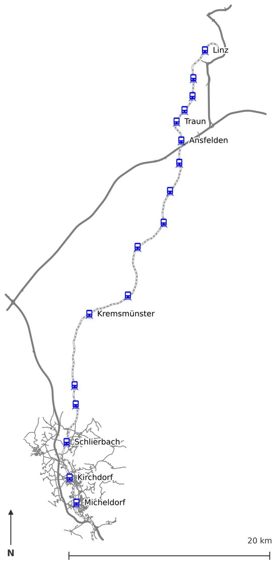
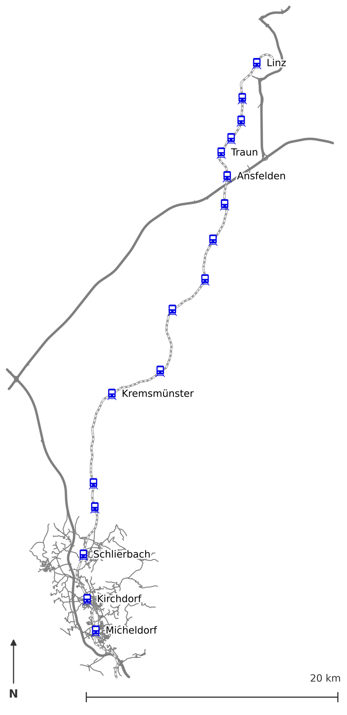
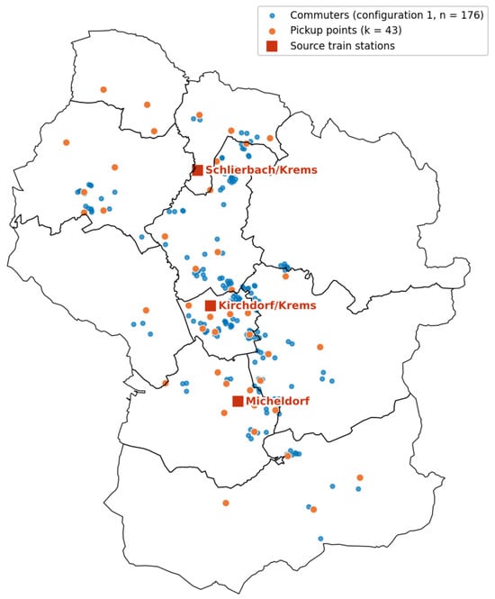
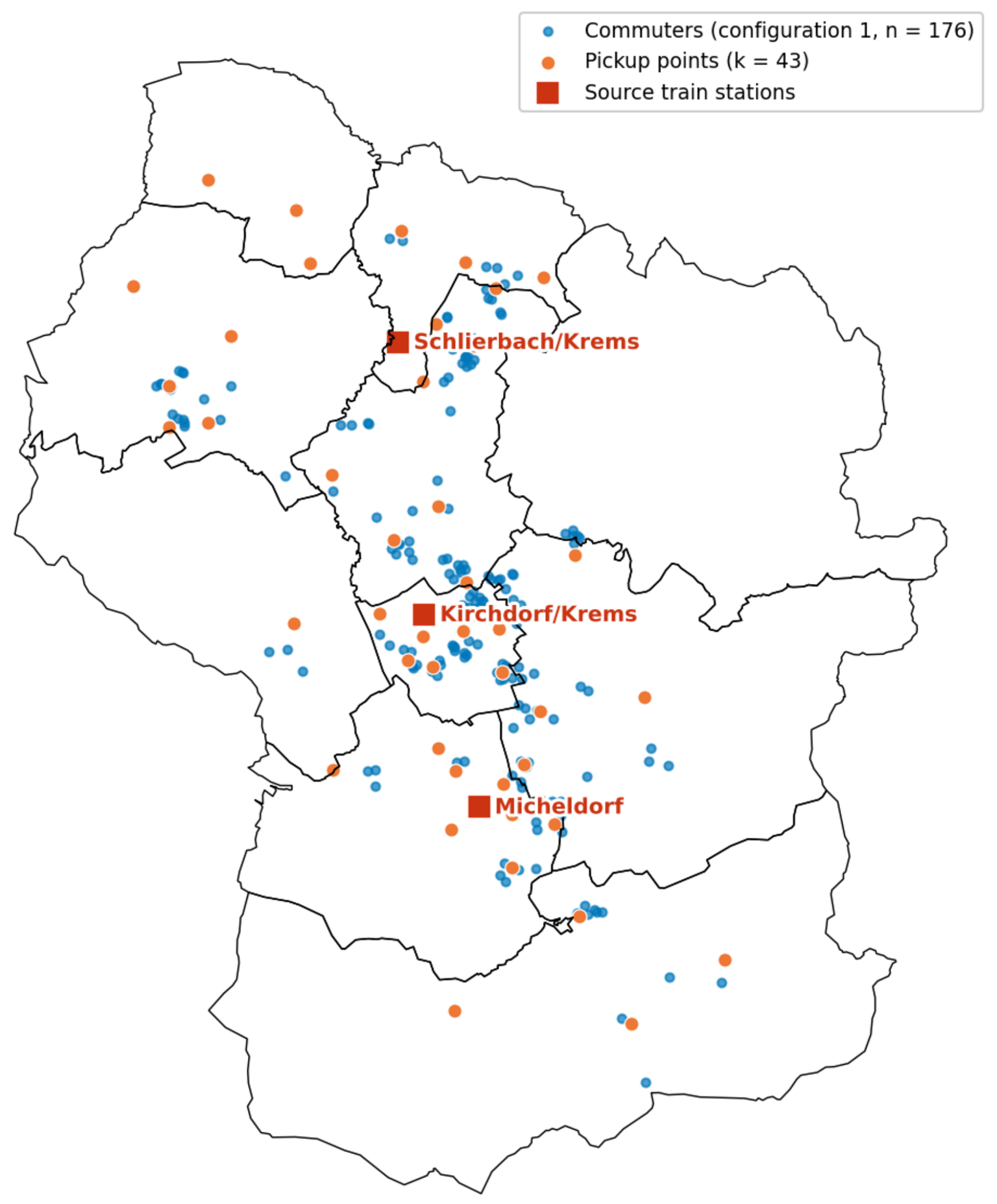
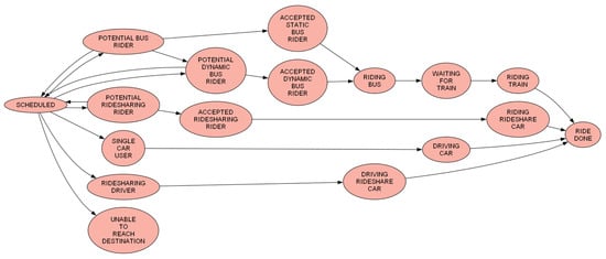
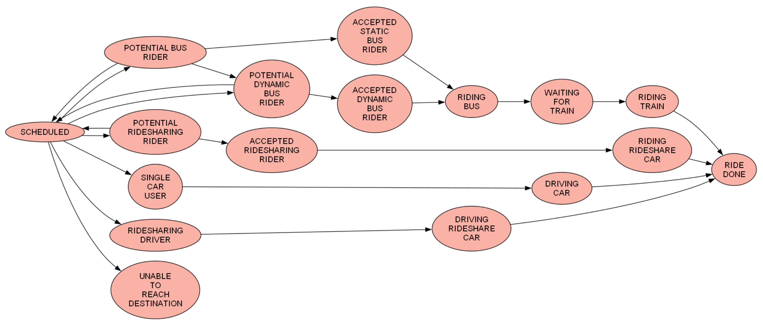
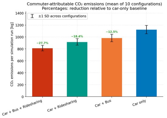
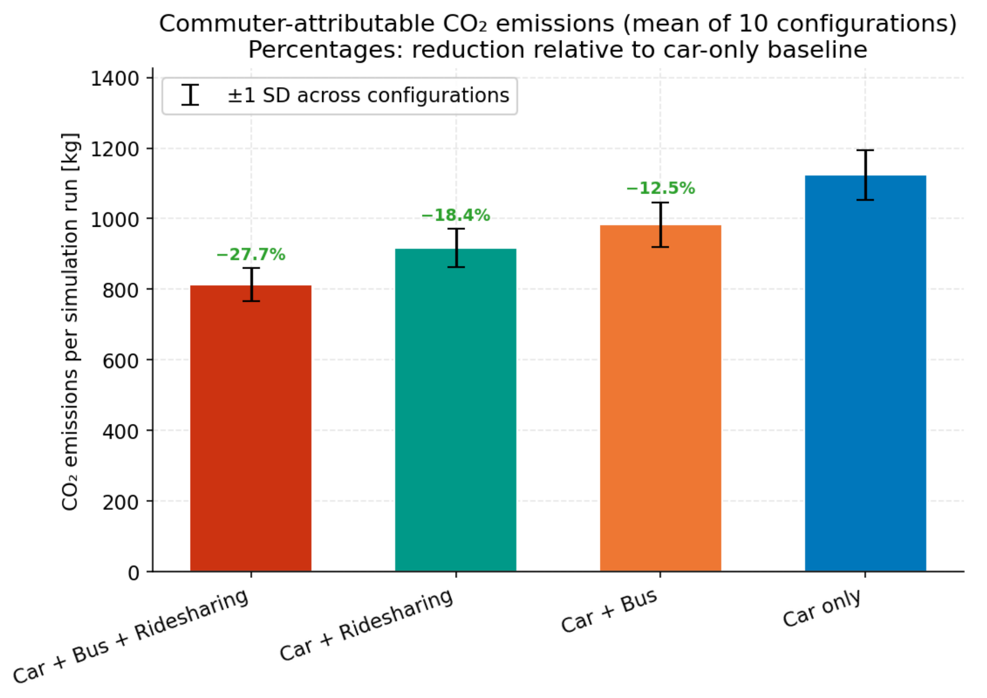
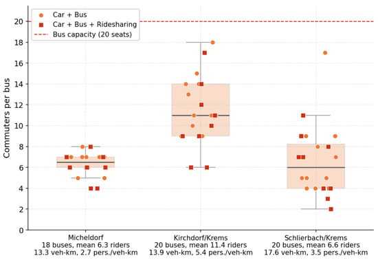
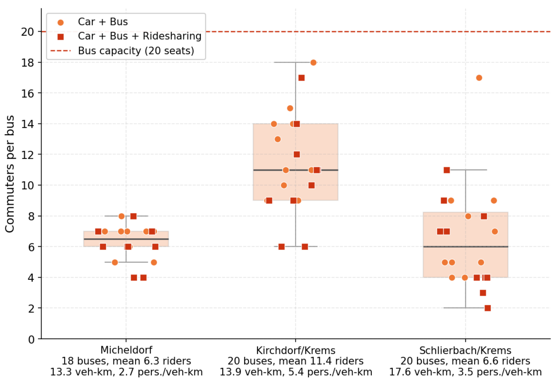
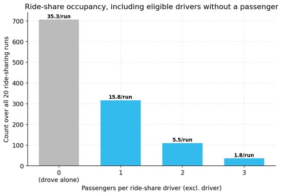
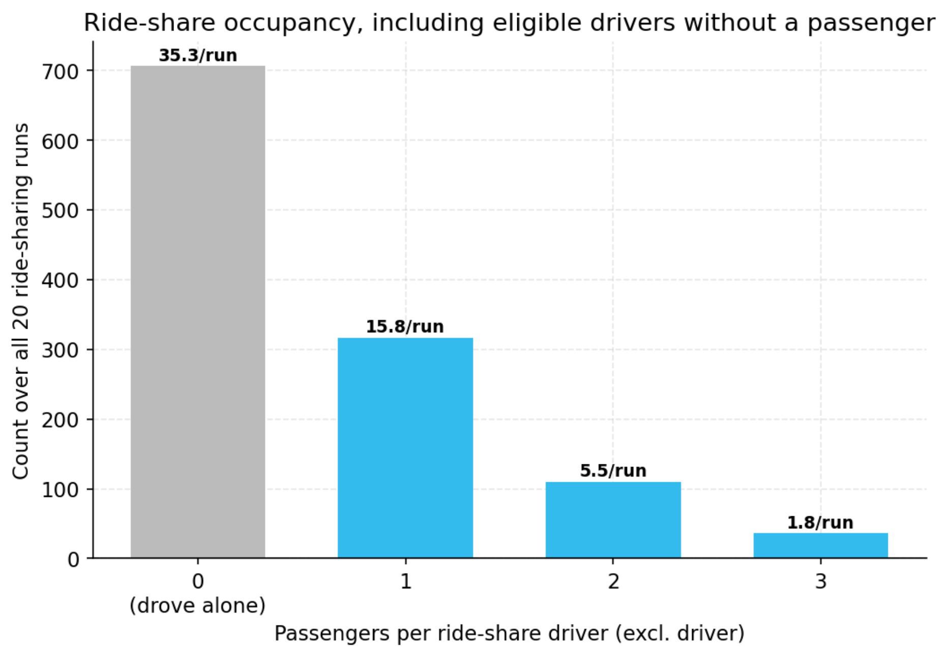
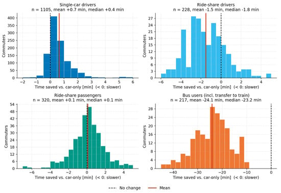
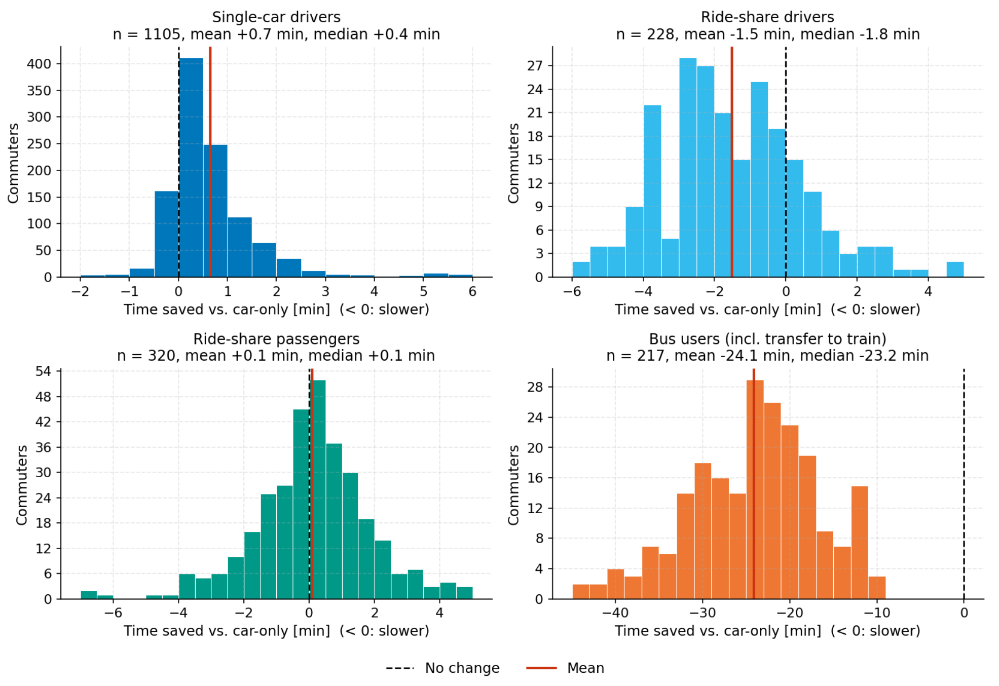
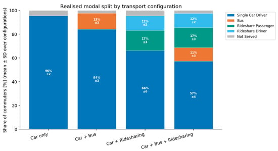
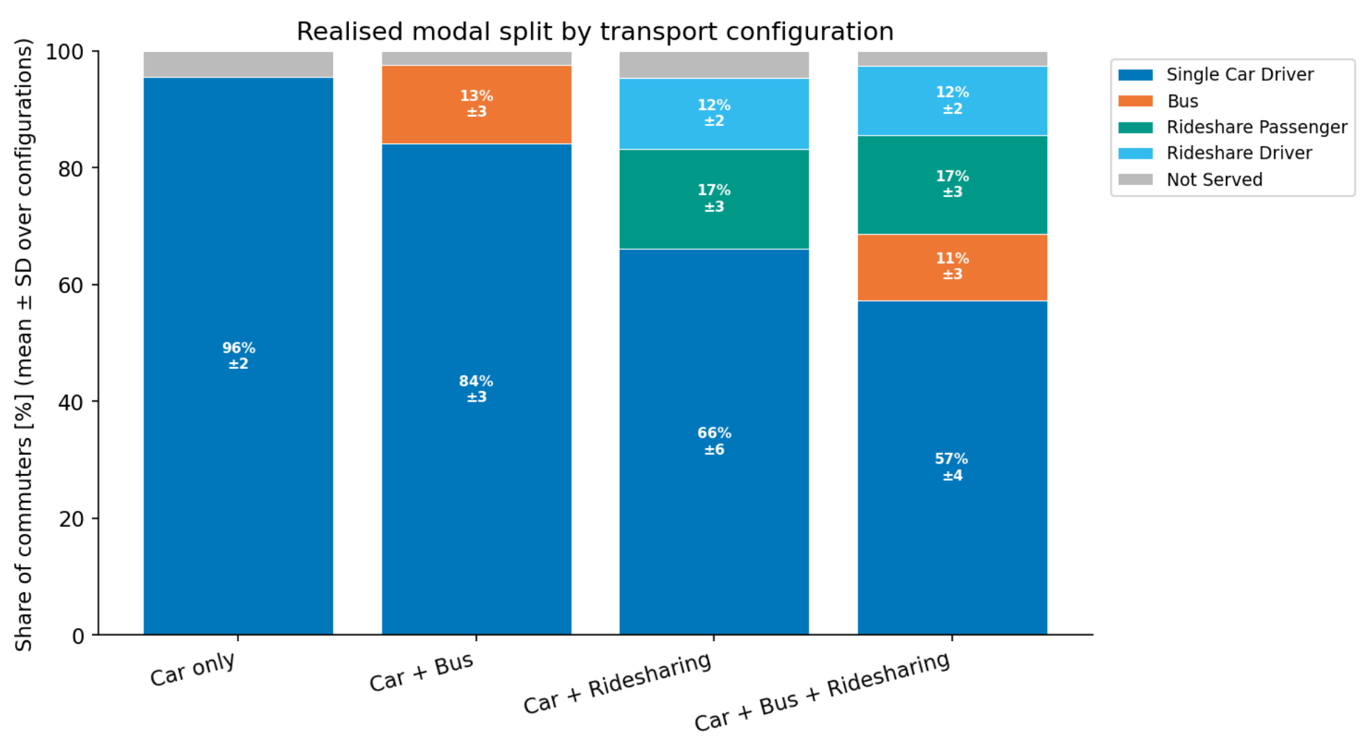
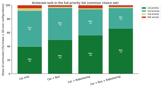
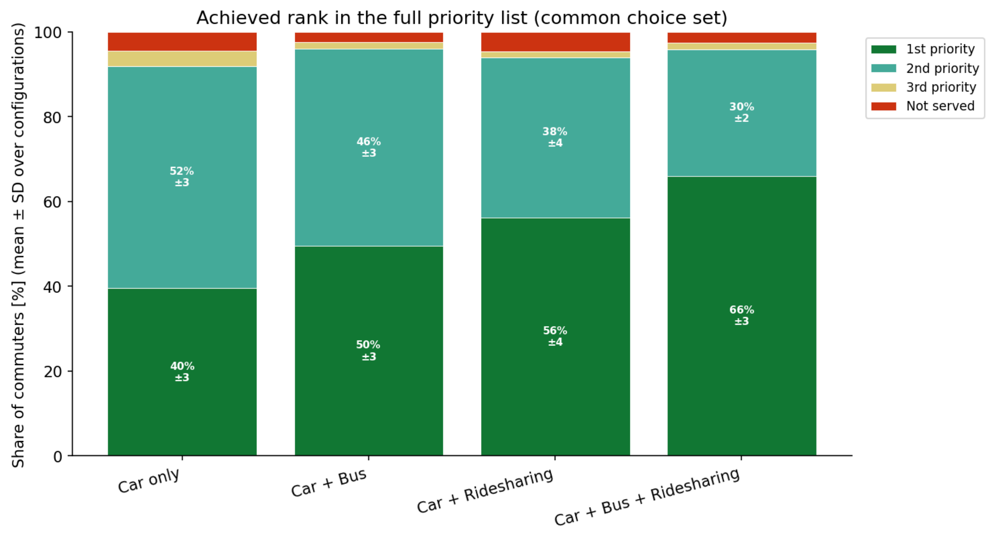

Disclaimer/Publisher’s Note: The statements, opinions and data contained in all publications are solely those of the individual author(s) and contributor(s) and not of MDPI and/or the editor(s). MDPI and/or the editor(s) disclaim responsibility for any injury to people or property resulting from any ideas, methods, instructions or products referred to in the content. |
© 2026 by the authors. Licensee MDPI, Basel, Switzerland. This article is an open access article distributed under the terms and conditions of the Creative Commons Attribution (CC BY) license.