Coordinated Dispatch for Partitioned Power Grids Under Extreme Weather with a Flexibility Supply–Demand Balance Approach

Abstract

To address the insufficient flexibility in power systems caused by renewable energy output uncertainty during extreme weather events, a coordinated source–network–load–storage (SNLS) dispatch method that combines a flexibility supply–demand balance approach with a partitioned grid framework is proposed to achieve the effective enhancement of operational resilience. Firstly, a convolution method is employed to aggregate net load forecast error distributions, and expected flexibility demand metrics are introduced to construct a probabilistic model of compound weather impacts, thereby improving flexibility requirement quantification. Secondly, uncertainties arising from extreme meteorological conditions are considered, and an integrated economic dispatch model for the partitioned grid is established based on chance-constrained reserves and regulation capability envelopes, in order to co-optimize generation costs, demand response, and expected flexibility insufficiency penalties. Then, inter-zone power exchange and spatiotemporal unit commitment dynamics are introduced to optimally redistribute spatial generation surpluses and load deficits, so that a system-wide flexibility supply–demand balance is enabled. Finally, simulations are conducted on the real-world Guangdong 500 kV transmission network under typhoon, heatwave, and rainstorm scenarios, and the results demonstrate the effectiveness of the proposed method in eliminating flexibility deficits, reducing total dispatch costs, and capturing distinct weather-adaptive operational patterns.

1. Introduction

Against the backdrop of the global energy transition and the advancement of carbon neutrality goals, power systems are shifting from traditional rigid supply–demand models toward flexible interactive architectures with a high penetration of renewable energy sources [1]. The inherent variability and uncertainty of wind and solar photovoltaic (PV) generation pose significant challenges to power system operation [2]. Extreme weather, like typhoons, heatwaves, or heavy rain, exacerbates these challenges considerably. During these storms, the actual renewable energy produced often misses the forecast by a wide margin. At the exact same time, people change how they use electricity. This creates a compound operational challenge characterized by a severe lack of flexibility [3,4]. For example, during the combined heatwave and drought that hit Southwest China in the summer of 2022, hydropower generation fell by more than 50%. Meanwhile, the demand for air conditioning pushed the nationwide load past 260 GW. In Sichuan province alone, the grid fell 17 GW short [5]. Such events underscore the necessity of incorporating flexibility stress induced by extreme weather into grid dispatch models [6].

The intersection of extreme weather and power system operation has attracted growing research attention. Nik et al. [4] provided a Nature Reviews perspective on climate-resilient net-zero power systems, emphasizing the compound risks of intensifying climate extremes coinciding with reduced renewable generation. Lin and Bie [3] comprehensively reviewed resilience concepts, assessment methods, and enhancement measures for power systems under severe weather. For typhoon events specifically, Zhang et al. [7] developed a two-stage stochastic programming framework for distribution network resilience enhancement by coordinating line hardening, DG placement, and mobile emergency generators. Wang et al. [8] proposed a data-driven spatial distributionally robust optimization approach for typhoon resilience validated on Hong Kong region data. Xu et al. [9] addressed stochastic unit commitment with high-penetration offshore wind in typhoon scenarios using a progressive hedging algorithm. However, these studies primarily focus on asset hardening and post-event recovery; few have investigated intra-event operational coordination—particularly the spatial propagation of wind generation surpluses and the associated flexibility dynamics across partitioned grid zones during typhoon passage. While operational coordination under extreme events remains underexplored, the coordinated dispatch of source, network, load, and storage (SNLS) under normal conditions has been widely investigated [10], providing a valuable methodological basis that can be extended to extreme weather scenarios.

Extensive research has been conducted on coordinated source–network–load–storage (SNLS) dispatch for distribution networks. Mi et al. [11] proposed a multi-timescale optimal dispatching strategy integrating SNLS interaction based on second-order cone programming (SOCP), achieving 18.28% economic improvement and 24.39% increase in renewable consumption on the IEEE 33-node system. Zhang et al. [12] developed a hierarchical optimization framework for SNLS under high PV penetration using an improved differential evolution algorithm. Fan et al. [13] reviewed how to plan integrated energy systems using coordinated source–network–load–storage (SNLS). They noted that handling uncertainty and timing are major areas that need more work. Also, Sun et al. [14] created a distributed method to help these flexible SNLS resources work together in smart grids. However, there is a common hurdle in all these SNLS models: the math. AC power flow equations create non-linear problems, and dealing with so many unknown variables at once requires building specialized mathematical solvers.

To handle the nonlinearity inherent in SNLS dispatch models, convex relaxation techniques—particularly SOCP relaxation—have been widely adopted to transform non-convex formulations into tractable convex forms [15]. Song et al. [16] proposed a chance-constrained economic dispatch model incorporating network flexibility against renewable uncertainties using Gaussian mixture models. Bhattacharya et al. [17] quantified flexibility requirements under forecast uncertainties for high-renewable systems. Building on the foundational branch flow model [18,19,20], researchers have developed robust energy management frameworks using mixed-integer SOCP for active distribution networks [21], coordinated active–reactive power optimization incorporating PV curtailment considerations [22], and robust dispatch methods leveraging four-quadrant energy storage output [23,24]. For uncertainty handling, stochastic optimization and robust optimization approaches have been extensively applied. Foundational works on flexibility evaluation [25,26] and flexibility enhancement through generation, storage, and demand response coordination [27,28,29] have established important methodological bases, though primarily focused on normal operating conditions rather than extreme weather scenarios.

To fill this research gap, this paper proposes a coordinated SNLS dispatch model with flexibility supply–demand balance for partitioned power grids under extreme weather conditions. The main contributions are: (1) We bridge probability convolution with a multi-timescale flexibility penalty and partitioned spatial coordination, creating a unified framework tailored for the compound uncertainties of extreme weather. (2) Through a novel four-scenario comparative analysis, we demonstrate that this integrated architecture eliminates extreme flexibility deficits while avoiding the severe over-conservatism (and associated cost surges) inherent in traditional robust optimization methods. (3) Empirical spatiotemporal discoveries: Applied to the real-world Guangdong 500 kV grid, the model reveals critical weather-adaptive operational patterns, most notably discovering a predictable 4 h spatiotemporal propagation lag of sequential generator decommitments that directly mirrors a typhoon’s physical translation velocity across the coast.

2. Materials and Methods

2.1. Overview

The proposed coordinated source–network–load–storage (SNLS) dispatch framework aims to enhance the resilience and economic efficiency of partitioned power grids under extreme weather conditions.

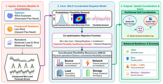
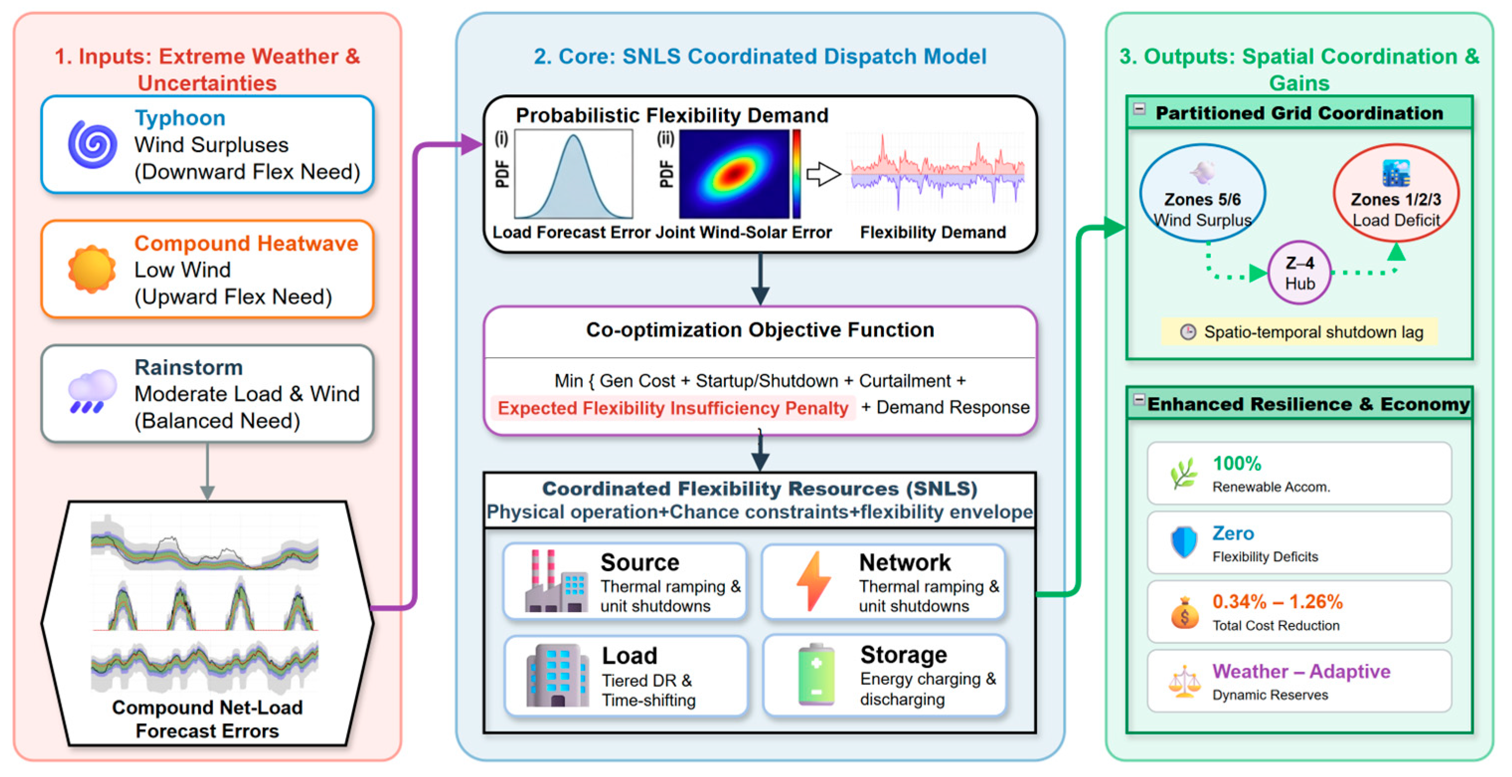
As shown in Figure 1, the proposed model transitions from traditional rigid dispatching paradigms to a flexibility-centric framework. We use probability to measure the complex forecasting errors caused by bad weather. If the system does not have enough flexibility, the model applies a direct penalty. To meet flexibility needs across different locations and times, the model links several tools together. It coordinates thermal plants and renewables (the source); limits on power flowing between grid zones (the network); load shedding and shifting power demand to different times (the load); and batteries (the storage). These coordinated mechanisms are integrated into a single MILP model. This ensures that the grid stays secure and adapts to the weather across different geographic zones.

Figure 1. Overall framework.

2.2. Objective Function

The objective is to minimize the total expected system cost over the dispatch horizon. The cost function comprises six components, each addressing a distinct operational consideration. The complete objective is:

$$\min \hspace{0.33em}{C}_{\mathrm{total}}={\displaystyle \sum _{t=1}^T\left(C_t^{\mathrm{ad}}+C_t^{\mathrm{ud}}+C_t^{\mathrm{cur}}+C_t^{\mathrm{shed}}+C_t^{\mathrm{sft}}+C_t^{\mathrm{flex}}\right)}$$

(1)

where $C_t^{\mathrm{ad}}$ is the generation cost of adjustable thermal units at time $t$; $C_t^{\mathrm{ud}}$ is the start-up and shutdown cost; $C_t^{\mathrm{cur}}$ is the penalty cost for curtailing renewable generation; $C_t^{\mathrm{shed}}$ is the compensation cost for tiered load shedding; $C_t^{\mathrm{sft}}$ is the compensation cost for time-shifting flexible loads; and $C_t^{\mathrm{flex}}$ is the expected flexibility insufficiency penalty.

(1)

Generation Cost

The generation cost of adjustable thermal units is modeled as a convex quadratic function of active power output, reflecting the increasing marginal cost characteristic of thermal generation. This formulation captures the efficiency penalty of operating units away from their optimal loading point and is standard in the unit commitment literature.

$$C_t^{\mathrm{ad}}={\displaystyle \sum _{i=1}^N\left[a_i{\left(P_{i,t}^{\mathrm{ad}}\right)}^2+b_i{P}_{i,t}^{\mathrm{ad}}+c_i\right]}$$

(2)

where $N$ is the total number of adjustable thermal generator units; $P_{i,t}^{\mathrm{ad}}\in {ℝ}^{+}$ is the active power output (MW) of unit $i$ during period $t$; and $a_i>0$ (CNY/MW²), $b_i$ (CNY/MW), and $c_i$ (CNY) are the quadratic, linear, and constant generation cost coefficients of unit $i$, respectively. The quadratic term $a_i{(P_{i,t}^{\mathrm{ad}})}^2$ dominates at high output levels, creating a natural incentive to distribute generation across multiple units rather than overloading a single cheap unit.

(2)

Start-up and Shutdown Cost

Thermal units incur fixed costs when transitioning between offline and online states. These costs reflect fuel consumption during boiler warm-up, additional maintenance wear from thermal cycling, and auxiliary power requirements during the start-up sequence. Accurate modeling of these transition costs is essential for commitment decisions, particularly during typhoon events where coordinated shutdowns are used to provide downward flexibility.

$$C_t^{\mathrm{ud}}={\displaystyle \sum _{i=1}^N\left({\tau }_i^{\mathrm{on}}{v}_{i,t}^{\mathrm{on}}+{\tau }_i^{\mathrm{off}}{v}_{i,t}^{\mathrm{off}}\right)}$$

(3)

where $v_{i,t}^{\mathrm{on}}\in \{0,1\}$ and $v_{i,t}^{\mathrm{off}}\in \{0,1\}$ are binary indicator variables: $v_{i,t}^{\mathrm{on}}=1$ if and only if unit $i$ transitions from offline ($u_{i,t-1}=0$) to online ($u_{i,t}=1$) at the beginning of period $t$, and $v_{i,t}^{\mathrm{off}}=1$ for the reverse transition. The parameters ${\tau }_i^{\mathrm{on}}$ and ${\tau }_i^{\mathrm{off}}$ (CNY per transition) are the unit-specific startup and shutdown cost coefficients. The relationship between these indicators and the commitment status $u_{i,t}$ is formally defined in Section 2.4.

(3)

Renewable Curtailment Penalty

While modern power dispatch practices are shifting away from strict administrative curtailment penalties, a linear penalty term is retained here as a mathematical proxy for resilience. During extreme weather, maximizing local, zero-marginal-cost renewable energy is vital to minimize reliance on vulnerable thermal fuel supply chains. This penalty ensures the solver exhausts all available spatial and demand-side flexibility resources before curtailing renewables, aligning with both resilience priorities and carbon reduction goals.

$$C_t^{\mathrm{cur}}={\tau }^{\mathrm{curt}}{\displaystyle \sum _{j=1}^M{P}_{j,t}^{\mathrm{curt}}}$$

(4)

where $M$ is the total number of renewable generation units (wind farms and PV plants); $P_{j,t}^{\mathrm{curt}}\ge 0$ is the curtailed active power (MW) of renewable unit $j$ during period $t$; and ${\tau }^{\mathrm{curt}}$ (CNY/MWh) is the unified curtailment penalty coefficient, set to a value sufficiently large (500 CNY/MWh in this study, comparable to the feed-in tariff) to ensure curtailment is the flexibility resource of absolute last resort.

(4)

Tiered Load Shedding Compensation

Demand response programs compensate consumers for voluntarily reducing or deferring their electricity consumption. To reflect the increasing inconvenience and economic impact of deeper curtailment, a four-tier compensation structure is adopted. Each successive tier allows a larger curtailment fraction but at a higher per-unit compensation rate, creating a convex increasing marginal cost of demand response that naturally limits excessive reliance on load shedding.

$$C_t^{\mathrm{shed}}={\displaystyle \sum _{m\in \mathcal{Q}}{\displaystyle \sum _{l=0}^3{\tau }_m^{\mathrm{shed},l}}}{P}_{m,t}^{\mathrm{shed},l}$$

(5)

where $\mathcal{Q}$ denotes the set of all network nodes; $l\in \{0,1,2,3\}$ indexes the four shedding tiers in order of increasing curtailment depth and compensation rate (Tier 0: minimal curtailment, lowest compensation; Tier 3: deep curtailment, highest compensation); ${\tau }_m^{\mathrm{shed},l}$ (CNY/MWh) is the compensation price at node $m$ for tier-$l$ load shedding; and $P_{m,t}^{\mathrm{shed},l}\ge 0$ (MW) is the amount of load shed at node $m$ during period $t$ under tier $l$. The tier-specific curtailment limits are defined in Section 3.4.

(5)

Load Time-Shift Compensation

In addition to pure curtailment, certain categories of flexible loads—such as industrial process heating, water pumping, and electric vehicle charging—can be rescheduled to different time periods without reducing total energy consumption. The compensation for this temporal rescheduling is proportional to the magnitude of the shifted load and the temporal distance of the displacement, reflecting the increasing inconvenience of larger time shifts.

$$C_t^{\mathrm{sft}}={\displaystyle \sum _{m\in \mathcal{Q}}\left[{\varphi }_m{\displaystyle \sum _{t^{\prime }=1}^T|}t-t^{\prime }|P_m^{\mathrm{LS}}(t,t^{\prime })\right]}$$

(6)

where $P_m^{\mathrm{LS}}(t,t^{\prime })\ge 0$ (MW) is the load shifted from original consumption period $t$ to new consumption period t’ at node $m$; $|t-t^{\prime }|$ is the absolute temporal displacement (in number of time periods $\Delta t$); and ${\varphi }_m$ (CNY/MWh per period) is the node-specific time-shift compensation coefficient. The total shifted-out load from each period is constrained in Section 3.4. Note that load shifted from $t$ to t’, t’ < t represents pre-heating or pre-cooling strategies.

(6)

Flexibility Insufficiency Penalty

A primary feature of the integrated model is the explicit quantification and penalization of expected flexibility insufficiency. Rather than treating flexibility as a hard constraint (which may lead to infeasibility under extreme conditions) or ignoring it entirely (which produces economically optimal but operationally fragile solutions), the model computes the expected magnitude of flexibility shortfall—the amount by which aggregate flexibility demand exceeds aggregate flexibility supply—and applies a penalty that internalizes the economic consequence of this inadequacy.

The flexibility insufficiency in each direction (upward and downward) is defined as the positive part of the demand–supply gap, aggregated over all relevant timescales. The penalty term is:

$$\begin{array}{l}{C}_t^{\mathrm{flex}}=c_f\left({\Delta }_{\mathrm{up},t}+{\Delta }_{\mathrm{down},t}\right),\hspace{1em}{\Delta }_{\mathrm{up},t}={\displaystyle \sum _{\tau \in \mathsf{\Phi }}\max }\left(0,\hspace{0.33em}{D}_{t+\tau }^{+}-{\displaystyle \sum _{i=1}^n{v}_{i,t+\tau }^{+}}\right),\hspace{1em}\\ {\Delta }_{\mathrm{down},t}={\displaystyle \sum _{\tau \in \mathsf{\Phi }}\max }\left(0,\hspace{0.33em}{D}_{t+\tau }^{-}-{\displaystyle \sum _{i=1}^n{v}_{i,t+\tau }^{-}}\right)\end{array}$$

(7)

where $c_f$ (CNY/MWh) is the flexibility insufficiency penalty coefficient—set sufficiently large (500 CNY/MWh), aligning with the empirical penalty caps and feed-in tariffs in the Guangdong power market; $\mathsf{\Phi }=\{{\tau }_1,{\tau }_2,\dots ,{\tau }_H\}$ is the set of timescales considered (15 min, 1 h, and 4 h in this study); $D_{t+\tau }^{+}$ and $D_{t+\tau }^{-}$ (MW) are the upward and downward flexibility demands at time scale $\tau$, quantified in Section 3.3; $n$ is the total number of flexibility-providing resources (generators, storage, and curtailable loads); and $v_{i,t+\tau }^{+}$, $v_{i,t+\tau }^{-}$ (MW) are the upward and downward flexibility supply capabilities of resource i at time scale\tau, defined through the regulation capability envelope in Section 3.4.

2.3. Flexibility Demand Quantification via Convolution

The flexibility demand is driven by the net load forecast error—the difference between the actual and predicted values of the residual load after subtracting renewable generation. Under extreme weather, both load and renewable forecasts exhibit elevated errors, and their combined effect must be quantified probabilistically. The following subsections develop the convolution-based quantification framework.

(1)

Net Load Definition

The system net load at each time period is defined as the total system load minus the aggregate forecasted renewable generation. This quantity represents the portion of load that must be served by adjustable resources (thermal generators and storage).

$$L_t^{\mathrm{net}}=L_t^{\mathrm{load}}-\left(P_{w,t}^{\mathrm{pred}}+P_{s,t}^{\mathrm{pred}}\right)$$

(8)

where $L_t^{\mathrm{load}}$ (MW) is the forecasted total system load (including transmission losses) at time $t$; $P_{w,t}^{\mathrm{pred}}$ and $P_{s,t}^{\mathrm{pred}}$ (MW) are the predicted aggregate wind and solar PV power outputs at time $t$, obtained from numerical weather prediction models. All three quantities are deterministic inputs to the day-ahead dispatch model.

(2)

Forecast Error Characterization

The load forecast error is modeled as a zero-mean normal distribution. This distributional assumption is theoretically justified by the Central Limit Theorem, as the aggregate system-level load error represents the summation of millions of independent, random deviations in individual consumer behaviors. The time-dependent variance ${\sigma }_{L,t}^2$ is estimated directly from actual historical extreme-weather operational data in Guangdong. The variance of the error distribution is estimated from historical forecast performance data and is typically larger during extreme weather due to the atypical load patterns induced by temperature extremes.

$$\Delta L_t^{\mathrm{load}}=L_t^{\mathrm{load},\mathrm{actual}}-L_t^{\mathrm{load}}~\mathcal{N}\left(0,\hspace{0.33em}{\sigma }_{L,t}^2\right)$$

(9)

where $\Delta L_t^{\mathrm{load}}$ (MW) is the load forecast error at time $t$; $L_t^{\mathrm{load},\mathrm{actual}}$ (MW) is the actual realized load (unknown at dispatch time); $\mathcal{N}(0,{\sigma }_{L,t}^2)$ denotes a normal distribution with zero mean and time-dependent variance ${\sigma }_{L,t}^2$, which is estimated from historical forecast error statistics conditioned on weather type.

Wind and solar forecast errors exhibit significant dependence under extreme weather conditions because both are driven by the same meteorological system. During typhoon passage, for instance, both wind and solar forecasts deviate in correlated ways as the cyclone circulation affects wind speed and cloud cover simultaneously. This joint dependence is captured through a bivariate probability distribution:

$$\Delta P_{w,t}=P_{w,t}^{\mathrm{actual}}-P_{w,t}^{\mathrm{pred}},\hspace{1em}\Delta P_{s,t}=P_{s,t}^{\mathrm{actual}}-P_{s,t}^{\mathrm{pred}},\hspace{1em}(\Delta P_{w,t},\hspace{0.33em}\Delta P_{s,t})~F_{w,s}(p_w,p_s)$$

(10)

where $\Delta P_{w,t}$ and $\Delta P_{s,t}$ (MW) are the wind and solar forecast errors at time $t$; $P_{w,t}^{\mathrm{actual}}$ and $P_{s,t}^{\mathrm{actual}}$ are the actual realized outputs; $F_{w,s}(p_w,p_s)$ is the joint cumulative distribution function (CDF) of wind and solar forecast errors, estimated empirically from historical extreme weather events using kernel density estimation or fitted parametric copula models.

(3)

Net Flexibility Demand Distribution

The total flexibility demand at each period is the net load fluctuation—the combined effect of load, wind, and solar forecast errors. Note that the macro-correlations induced by extreme weather (e.g., heatwaves driving high load and low wind) are already captured by the deterministic day-ahead forecasts. Assuming conditional independence strictly between the residual forecast errors of load (driven by consumption behaviors) and renewables (driven by micro-meteorological noise), the probability density function of the net flexibility demand is obtained via convolution.

$$D_t^{\mathrm{flex}}=\Delta L_t^{\mathrm{load}}-\left(\Delta P_{w,t}+\Delta P_{s,t}\right)$$

(11)

where $D_t^{\mathrm{flex}}$ (MW) is the net load fluctuation at time $t$, representing the instantaneous flexibility regulation demand. Positive values indicate a need for upward flexibility (generation increase or load reduction), while negative values indicate a need for downward flexibility (generation reduction or load increase).

$$f_{D,t}(d)=\left(f_{\Delta L,t}*f_{-(\Delta P_w+\Delta P_s),t}\right)(d)={\displaystyle {\int }_{-\infty }^{+\infty }{f}_{\Delta L,t}}(\tau )\hspace{0.33em}{f}_{-(\Delta P_w+\Delta P_s),t}(d-\tau )\hspace{0.33em}d\tau$$

(12)

where $f_{D,t}(d)$ is the probability density function (PDF) of $D_t^{\mathrm{flex}}$ evaluated at value $d$; $f_{\Delta L,t}$ is the PDF of the load forecast error (normal density with variance ${\sigma }_{L,t}^2$); $f_{-(\Delta P_w+\Delta P_s),t}$ is the PDF of the negative of the combined wind–solar forecast error, obtained by transforming the joint distribution $F_{w,s}$; and * denotes the convolution operator. The integration is performed numerically using discretized PDF representations with a resolution of 1 MW.

(4)

Expected Upward and Downward Flexibility Demand

The expected upward flexibility demand is the mean of the positive part of the net flexibility demand distribution—intuitively, the average amount by which the net load is expected to exceed its forecasted value, requiring additional upward ramping capability. The expected downward flexibility demand is defined analogously for the negative part.

$$E[D_t^{\mathrm{up}}]={\displaystyle {\int }_0^{+\infty }d}\cdot f_{D,t}(d)dd,\hspace{1em}\hspace{1em}E[D_t^{\mathrm{down}}]={\displaystyle {\int }_{-\infty }^0(-d)}\cdot f_{D,t}(d)dd$$

(13)

where $E[D_t^{\mathrm{up}}]\ge 0$ (MW) is the expected upward flexibility requirement—the mean magnitude of net load increases beyond the forecast; $E[D_t^{\mathrm{down}}]\ge 0$ (MW) is the expected downward flexibility requirement—the mean magnitude of net load decreases below the forecast. Both quantities are non-negative by construction.

(5)

Multi-Timescale Flexibility Demand

Flexibility requirements manifest across multiple timescales. Within a single 15 min dispatch interval, the concern is the instantaneous mismatch; over a 4 h window, the concern is the accumulated energy imbalance. To capture this multi-scale nature, the flexibility demand at timescale au is computed as the maximum net load excursion over all rolling windows of duration au within the planning horizon.

$$D_{t,\tau }^{+}={\max }_{j\in [t,t+\tau )}\max (0,\hspace{0.33em}{\max }_{k\in [j+\Delta t,t+\tau )}E[D_k^{\mathrm{up}}]-L_{\mathrm{net},j})$$

(14)

where $D_{t,\tau }^{+}$ (MW) is the upward flexibility demand at time $t$ for timescale $\tau$; the inner maximization over $k\in [j+\Delta t,t+\tau )$ computes the maximum expected upward flexibility requirement within the sub-window starting at $j+\Delta t$ and ending at $t+\tau$; the outer maximization over $j\in [t,t+\tau )$ ensures that the demand covers the most adverse starting point within the window. $L_{\mathrm{net},j}$ is the forecasted net load at period $j$. The downward demand $D_{t,\tau }^{-}$ is defined analogously: $D_{t,\tau }^{-}={\max }_{j\in [t,t+\tau )}\max (0,L_{\mathrm{net},j}-{\min }_{k\in [j+\Delta t,t+\tau )}E[D_k^{\mathrm{down}}])$.

The per-timescale demands are then aggregated into the quantities $D_t^{+}$ and $D_t^{-}$ that appear in the flexibility penalty term (Section 3.2) by taking the maximum demand across all relevant time scales at each period:

$$D_t^{+}={\max }_{\tau \in \mathsf{\Phi }}{D}_{t,\tau }^{+},\hspace{1em}\hspace{1em}{D}_t^{-}={\max }_{\tau \in \mathsf{\Phi }}{D}_{t,\tau }^{-}$$

(15)

where $\mathsf{\Phi }=\{15\min ,1\mathrm{h},4\mathrm{h}\}$ is the set of time scales considered. This aggregation ensures that the dispatch model maintains adequate flexibility to handle the most demanding timescales at each period.

2.4. Constraint Framework

The objective function minimization is subject to a comprehensive set of constraints that collectively define the feasible operating region of the partitioned power grid. These constraints span regulation capability envelopes, demand response limits, chance-constrained reserves, power flow physics, and the operational characteristics of generators and energy storage devices.

(1)

Regulation Capability Envelope Constraints

Each flexibility-providing resource $i$ is characterized by a regulation capability envelope that defines, for every time step and timescale, the maximum upward and downward flexibility it can supply. The envelope is bounded by four physical limits: the minimum and maximum power output, the finite ramp rate, and the available energy capacity (for storage) or fuel inventory (for generators). At a given dispatch time $k+n$ and timescale, the following constraints must hold:

$$\left\{\begin{array}{ll}{g}_i^{\min }\le v_i^{+}(k+n+\tau )\le g_i(k+n),\hfill & g_i(k+n)\le v_i^{+}(k+n+\tau )\le g_i^{\max }\hfill \\ -\tau R_i\le v_i^{-}(k+n+\tau )-g_i(k+n)\le 0,\hfill & 0\le v_i^{-}(k+n+\tau )-g_i(k+n)\le \tau R_i\hfill \\ v_i^{+}(k+n+\tau )\tau +W(k+n)\le W_i^{\max },\hfill & W(k+n)-v_i^{-}(k+n+\tau )\tau \ge W_i^{\min }\hfill \end{array}\right.$$

(16)

where $g_i(k+n)$ (MW) is the scheduled (baseline) power output of resource $i$ at time step $k+n$, obtained from the unit commitment solution; $g_i^{\min }$ and $g_i^{\max }$ (MW) are the minimum stable generation and maximum rated capacity of resource $i$; $v_i^{+}(k+n+\tau )$ and $v_i^{-}(k+n+\tau )$ (MW) are the upward and downward flexibility supply that resource $i$ can provide at time $k+n$ sustained over time scale $\tau$; $R_i$ (MW per unit time) is the maximum ramp rate; $W(k+n)$ (MWh) is the available energy reserve (state of charge for storage, fuel inventory for thermal units) at time $k+n$; and $W_i^{\min }$ and $W_i^{\max }$ (MWh) are the minimum and maximum energy limits. The first two inequality pairs enforce power and ramping limits; the last two enforce energy capacity limits over the sustained duration $\tau$.

(2)

Tiered Demand Response Constraints

The load shedding at each tier is limited by a tier-specific maximum curtailment ratio. The tiered structure ensures that deep curtailment (higher tiers) with greater consumer impact is only activated after shallower, lower-cost tiers have been exhausted, reflecting the convex increasing marginal disutility of demand response.

$$0\le P_{m,t}^{\mathrm{shed},l}\le {\alpha }_{m,t}^{L,l}{\overline{P}}_{m,t}^L,\hspace{1em}\forall t\in [1,T],\hspace{0.33em}\forall m\in \mathcal{Q},\hspace{0.33em}\forall l\in \{0,1,2,3\}$$

(17)

where ${\overline{P}}_{m,t}^L$ (MW) is the baseline (pre-demand-response) load at node $m$ during period $t$; ${\alpha }_{m,t}^{L,l}\in [0,1]$ is the maximum fraction of baseline load that can be shed at tier $l$, with the nesting condition $0\le {\alpha }^{L,0}<{\alpha }^{L,1}<{\alpha }^{L,2}<{\alpha }^{L,3}\le 1$. Typical values used in this study are $\{0.05,0.10,0.15,0.20\}$ for Tiers 0–3 respectively.

For time-shiftable loads, the total power shifted out of any period must not exceed the shiftable capacity at that node and period. Note that load shifted into a period increases the net load in that period, which is accounted for in the nodal power balance through the net load expectation term.

$$0\le {\displaystyle \sum _{t^{\prime }=1}^T{P}_m^{\mathrm{LS}}}(t,t^{\prime })\le {\alpha }_{m,t}^{\mathrm{LS}}{\overline{P}}_{m,t}^L,\hspace{1em}\forall t\in [1,T],\hspace{0.33em}\forall m\in \mathcal{Q}$$

(18)

where ${\alpha }_{m,t}^{\mathrm{LS}}\in [0,1]$ is the maximum fraction of baseline load at node $m$ during period $t$ that is eligible for time-shifting (set to 0.15 in this study). The summation over t’ aggregates all load shifted from period $t$ to any other period.

(3)

Chance-Constrained Reserve Capacity

To ensure that the system maintains sufficient reserve capacity to absorb forecast errors with high probability, chance constraints are formulated for both upward and downward reserves. The net load at each node, after accounting for demand response and renewable curtailment, is modeled as a Gaussian random variable—an approximation justified by the central limit theorem when multiple independent uncertainty sources are combined.

The mean of the net load distribution is the expected net load, which incorporates the baseline load forecast minus demand response adjustments and renewable generation net of curtailment:

$${\mu }_{m,t}^{\mathrm{net}}=\left[{\mu }_{m,t}^L-{\displaystyle {\displaystyle \sum _{l=0}^3}{P}_{m,t}^{\mathrm{shed},l}}-{\displaystyle {\displaystyle \sum _{t^{\prime }=1}^T}(}{P}_m^{\mathrm{LS}}(t,t^{\prime })-P_m^{\mathrm{LS}}(t^{\prime },t))\right]-{\displaystyle \sum _{j\in {\mathcal{R}}_m}(}{\mu }_{j,t}^{\mathrm{re}}-P_{j,t}^{\mathrm{curt}})$$

(19)

where ${\mu }_{m,t}^L$ (MW) is the mean (baseline forecast) load at node $m$ during period $t$; ${\mathcal{R}}_m$ is the set of renewable units connected at node $m$; ${\mu }_{j,t}^{\mathrm{re}}$ (MW) is the forecasted (mean) output of renewable unit $j$; $P_{j,t}^{\mathrm{curt}}$ (MW) is the curtailed output; the term $(P_m^{\mathrm{LS}}(t,t^{\prime })-P_m^{\mathrm{LS}}(t^{\prime },t))$ represents the net load change from time-shifting: load shifted out of $t$ ($P_m^{\mathrm{LS}}(t,t^{\prime })$) reduces net load at $t$, while load shifted into $t$ from other periods ($P_m^{\mathrm{LS}}(t^{\prime },t)$) increases it.

The standard deviation of the net load is obtained by summing the variances of the independent load and renewable forecast errors:

$${\sigma }_{m,t}^{\mathrm{net}}=\sqrt{{({\sigma }_{m,t}^L)}^2+{\displaystyle \sum _{j\in {\mathcal{R}}_m}(}{\sigma }_{j,t}^{\mathrm{re}}{)}^2},\hspace{1em}\forall m\in \mathcal{Q},\hspace{0.33em}\forall t\in [1,T]$$

(20)

where ${\sigma }_{m,t}^L$ (MW) is the standard deviation of the load forecast error at node $m$; ${\sigma }_{j,t}^{\mathrm{re}}$ (MW) is the standard deviation of the forecast error of renewable unit $j$. The additivity of variances follows from the independence assumption between load and renewable forecast errors.

With the net load distribution characterized, the chance constraints require that the available reserve capacity exceeds the net load deviation with a prescribed confidence level $1-\beta$, where $\beta$ is the acceptable risk of reserve inadequacy. The chance constraints (Equation (21)) serve as static hard boundaries, ensuring sufficient nodal reserve capacity to cover expected errors with 95% confidence. Conversely, the flexibility penalty (Equation (7)) serves as a dynamic soft constraint that enforces multi-timescale (15 min, 1 h, 4 h) ramping capabilities and economically prices the remaining 5% extreme tail risks. They act complementarily.

$$\mathrm{Pr}[P_{m,t}^{\max }-P_{m,t}^{\mathrm{net}}\ge R_{m,t}^{+}]\ge 1-{\beta }^{+},\hspace{1em}\hspace{1em}\mathrm{Pr}[P_{m,t}^{\mathrm{net}}-P_{m,t}^{\min }\ge R_{m,t}^{-}]\ge 1-{\beta }^{-},\hspace{1em}\forall m,\hspace{0.33em}\forall t$$

(21)

where $\mathrm{Pr}[\cdot ]$ denotes probability; ${\beta }^{+}={\beta }^{-}=0.05$ are the risk tolerance parameters, corresponding to a 95% confidence level, aligning with standard grid operational protocols; $R_{m,t}^{+}$ and $R_{m,t}^{-}$ (MW) are the upward and downward reserve capacities scheduled at node $m$ during period $t$; $P_{m,t}^{\max }={\displaystyle \sum _{i\in {\mathcal{G}}_m}{u}_{i,t}}{\lambda }_i^{\max }$ (MW) is the maximum possible generation output at node $m$ if all committed units operate at full capacity; and $P_{m,t}^{\min }={\displaystyle \sum _{i\in {\mathcal{G}}_m}{u}_{i,t}}{\lambda }_i^{\min }$ (MW) is the corresponding minimum output. Under the Gaussian assumption, these chance constraints admit an exact deterministic reformulation: $R_{m,t}^{+}\ge {\mu }_{m,t}^{\mathrm{net}}+z_{1-{\beta }^{+}}{\sigma }_{m,t}^{\mathrm{net}}-P_{m,t}^{\max }$, where $z_{1-{\beta }^{+}}$ is the $(1-{\beta }^{+})$ quantile of the standard normal distribution.

Furthermore, while the deterministic reformulation relies on a Gaussian assumption that may weaken in the non-Gaussian, heavy-tailed extremes of severe weather, this structural vulnerability is strictly mitigated by the model’s dual-layer architecture. The chance constraints secure the 95% static baseline capacity, while the dynamic flexibility penalty (Equation (7)) is specifically co-optimized to manage the remaining 5% severe tail risks, ensuring overall model reliability.

(4)

DC Power Flow and Nodal Power Balance

The DC power flow approximation is adopted for the transmission network, offering linear expressions that enable an efficient solution of the large-scale mixed-integer programming problem. This approximation is well justified for the 500 kV transmission system studied here, where the resistance-to-reactance ratio is typically below 0.1 and voltage magnitude variations are tightly controlled within +/−5% of nominal.

$$P_{m,t}^{\mathrm{sp}}={\displaystyle \sum _{n\in {\mathcal{N}}_m,n\ne m}\frac{{\theta }_{m,t}-{\theta }_{n,t}}{x_{mn}}},\hspace{1em}\hspace{1em}\left|{\displaystyle \frac{{\theta }_{m,t}-{\theta }_{n,t}}{x_{mn}}}\right|\le F_{mn}^{\max },\hspace{1em}\forall m\in \mathcal{Q},\hspace{0.33em}\forall n\in {\mathcal{N}}_m,\hspace{0.33em}\forall t$$

(22)

where $P_{m,t}^{\mathrm{sp}}$ (MW) is the net active power injection from the transmission network into node $m$ during period $t$; ${\mathcal{N}}_m$ is the set of nodes directly connected by transmission lines to node $m$; ${\theta }_{m,t}$ and ${\theta }_{n,t}$ (radians) are the voltage phase angles at nodes $m$ and $n$; $x_{mn}$ (p.u.) is the series reactance of the line connecting nodes $m$ and $n$; and $F_{mn}^{\max }$ (MW) is the thermal capacity limit of the line, reflecting the maximum continuous current rating.

At each node, the active power balance must be maintained between net generation, storage discharge, network imports, and the expected net load:

$$P_{m,t}^{\mathrm{sp}}+{\displaystyle \sum _{k\in {\mathcal{S}}_m}{P}_{k,t}^{\mathrm{es}}}+{\displaystyle \sum _{i\in {\mathcal{G}}_m}{P}_{i,t}^{\mathrm{ad}}}=\mathbb{E}[P_{m,t}^{\mathrm{net}}],\hspace{1em}\forall m\in \mathcal{Q},\hspace{0.33em}\forall t\in [1,T]$$

(23)

where ${\mathcal{S}}_m$ is the set of energy storage units connected at node $m$; ${\mathcal{G}}_m$ is the set of adjustable generators at node $m$; $P_{k,t}^{\mathrm{es}}$ (MW) is the net power output of storage unit $k$, conventionally positive for discharging and negative for charging; and $\mathbb{E}[P_{m,t}^{\mathrm{net}}]={\mu }_{m,t}^{\mathrm{net}}$ (MW) is the expected net load defined in Section 3.4.

(5)

Adjustable Generator Operational Constraints

The commitment status of each adjustable generator is represented by a binary variable $u_{i,t}\in \{0,1\}$, where $u_{i,t}=1$ indicates that unit $i$ is online (synchronized and connected to the grid) during period $t$, and $u_{i,t}=0$ indicates the offline state. The startup and shutdown operation indicators are derived from transitions in the commitment status between consecutive periods.

$$v_{i,t}^{\mathrm{on}}=\max (u_{i,t}-u_{i,t-1},\hspace{0.33em}0)\hspace{1em}\hspace{1em}{v}_{i,t}^{\mathrm{off}}=\max (u_{i,t-1}-u_{i,t},\hspace{0.33em}0),\hspace{1em}\forall t\in [2,T],\hspace{0.33em}\forall i$$

(24)

where By construction, $v_{i,t}^{\mathrm{on}}=1$ if and only if unit $i$ transitions from offline to online at period $t$, and $v_{i,t}^{\mathrm{off}}=1$ for the reverse transition. For the initial period ($t=1$), the values $v_{i,1}^{\mathrm{on}}$ and $v_{i,1}^{\mathrm{off}}$ are specified based on the known initial commitment status. This formulation is linearized in the MILP implementation using standard big-M techniques.

When online, the generator output is bounded between the minimum stable generation and the maximum rated capacity. When offline, the output is forced to zero:

$$u_{i,t}{\lambda }_i^{\min }\le P_{i,t}^{\mathrm{ad}}\le u_{i,t}{\lambda }_i^{\max },\hspace{1em}\forall i,\hspace{0.33em}\forall t\in [1,T]$$

(25)

where ${\lambda }_i^{\min }$ (MW) is the minimum stable generation level—the lowest output at which the unit can operate continuously without combustion instability or excessive emissions; ${\lambda }_i^{\max }$ (MW) is the maximum continuous rated capacity. The product $u_{i,t}{\lambda }_i^{\min }$ ensures thatthe constraint is active only when the unit is online.

Inter-temporal ramping constraints limit the rate of change in generator output, reflecting the physical inertia and thermal stress limitations of the prime mover. These constraints are the primary source of temporal coupling in the dispatch problem and define the ramping component of flexibility provision.

$$\begin{array}{l}{P}_{i,t}^{\mathrm{ad}}-P_{i,t-1}^{\mathrm{ad}}\le u_{i,t}{\lambda }_i^{\mathrm{up}}+(1-u_{i,t}){\lambda }_i^{\max },\hspace{1em}\hspace{1em}\\ P_{i,t-1}^{\mathrm{ad}}-P_{i,t}^{\mathrm{ad}}\le u_{i,t-1}{\lambda }_i^{\mathrm{dn}}+(1-u_{i,t-1}){\lambda }_i^{\max },\hspace{1em}\forall i,\hspace{0.33em}\forall t\in [2,T]\end{array}$$

(26)

where ${\lambda }_i^{\mathrm{up}}$ and ${\lambda }_i^{\mathrm{dn}}$ (MW per period $\Delta t$) are the maximum upward and downward ramp rates of unit $i$ over one time step. The additional terms $(1-u_{i,t}){\lambda }_i^{\max }$ and $(1-u_{i,t-1}){\lambda }_i^{\max }$ relax the ramping constraint during online/offline transitions, allowing the unit to start up from zero or shut down to zero without violating ramp limits.

(6)

Energy Storage Operational Constraints

Energy storage systems (pumped hydro and battery storage) provide critical temporal flexibility by decoupling the timing of generation and consumption. The storage model distinguishes between the charging and discharging processes, each with its own efficiency factor, and tracks the stored energy level across consecutive periods.

The net power output of a storage unit is the difference between discharging and charging power, with the convention that positive values represent net discharge (power injection into the grid).

$$P_{k,t}^{\mathrm{es}}=P_{k,t}^{\mathrm{dis}}-P_{k,t}^{\mathrm{cha}},\hspace{1em}{P}_{k,t}^{\mathrm{dis}}\ge 0,\hspace{0.33em}{P}_{k,t}^{\mathrm{cha}}\ge 0,\hspace{1em}\forall k\in \mathcal{S},\hspace{0.33em}\forall t$$

(27)

where $P_{k,t}^{\mathrm{dis}}$ and $P_{k,t}^{\mathrm{cha}}$ (MW) are the discharging and charging power of storage unit $k$ during period $t$. These are non-negative decision variables; the storage cannot simultaneously charge and discharge within a single period—a condition enforced implicitly by the convexity of the cost function and the efficiency losses, which make simultaneous charging and discharging strictly suboptimal.

The stored energy evolves according to a linear difference equation that accounts for conversion losses during both charging and discharging:

$$E_{k,t}=E_{k,t-1}+{\eta }_k^{\mathrm{cha}}{P}_{k,t}^{\mathrm{cha}}\Delta t-{\displaystyle \frac{P_{k,t}^{\mathrm{dis}}}{{\eta }_k^{\mathrm{dis}}}}\Delta t,\hspace{1em}{E}_k^{\min }\le E_{k,t}\le E_k^{\max },\hspace{1em}\forall k\in \mathcal{S},\hspace{0.33em}\forall t\in [2,T]$$

(28)

where $E_{k,t}$ (MWh) is the stored energy at the end of period $t$; ${\eta }_k^{\mathrm{cha}}\in (0,1]$ is the round-trip charging efficiency (ratio of stored energy to input electrical energy); ${\eta }_k^{\mathrm{dis}}\in (0,1]$ is the discharging efficiency (ratio of output electrical energy to extracted stored energy); $E_k^{\max }$ (MWh) is the rated energy capacity; $E_k^{\min }$ (MWh) is the minimum allowable stored energy, typically set by depth-of-discharge limits (e.g., 20\% of $E_k^{\max }$ for Li-ion batteries). The initial energy $E_{k,1}$ is specified as an input parameter.

The charging and discharging power are bounded by the converter ratings, which are typically symmetric for battery storage but may be asymmetric for pumped hydro:

$$0\le P_{k,t}^{\mathrm{dis}}\le {\delta }_k^{\mathrm{dis}},\hspace{1em}\hspace{1em}0\le P_{k,t}^{\mathrm{cha}}\le {\delta }_k^{\mathrm{cha}},\hspace{1em}\hspace{1em}{P}_{k,t}^{\mathrm{cha}}•P_{k,t}^{\mathrm{dis}}=0\hspace{1em}\forall k\in \mathcal{S},\hspace{0.33em}\forall t$$

(29)

where ${\delta }_k^{\mathrm{dis}}$ and ${\delta }_k^{\mathrm{cha}}$ (MW) are the maximum discharging and charging power ratings of storage unit $k$, determined by the power conversion system (inverter for batteries, turbine/pump ratings for pumped hydro).

(7)

Renewable Curtailment Constraints

The curtailed renewable power at each unit is bounded between zero and the available (forecasted) renewable output. The high penalty coefficient $a{u}^{extcurt}$ in the objective function ensures that curtailment is utilized only after all other flexibility resources—inter-zone power exchange, energy storage, demand response, and generator ramping—have been exhausted.

$$0\le P_{j,t}^{\mathrm{curt}}\le P_{j,t}^{\mathrm{re}},\hspace{1em}\forall j\in \{1,\dots ,M\},\hspace{0.33em}\forall t\in [1,T]$$

(30)

where $P_{j,t}^{\mathrm{re}}$ (MW) is the available (forecasted) renewable power output of unit $j$ at time $t$. This variable is an exogenous input to the dispatch model, obtained from the numerical weather prediction-based renewable forecasting system.

3. Results

3.1. System Description and Parameter Settings

The case study is based on the Guangdong 500 kV AC transmission network, comprising 95 nodes, 154 thermal power plants (85.6 GW), 13 nuclear plants (16.1 GW), 5 hydroelectric plants (3.2 GW), 9 pumped storage plants (9.6 GW), 75 wind farms (18.7 GW), and 46 PV plants (12.4 GW). The system is partitioned into six geographic zones: Zone 1—Northeast Pearl River Delta (load center, ~22% of the total load), Zone 2—Southeast Pearl River Delta (~18%), Zone 3—Northwest Pearl River Delta (~15%), Zone 4—Southwest Pearl River Delta (transmission hub, ~16%), Zone 5—Eastern Guangdong (wind-rich, ~15%), and Zone 6—Western Guangdong (wind-rich, ~14%). Zones 5 and 6 collectively host approximately 65% of the system’s total wind capacity (12.2 GW out of 18.7 GW).

Three representative extreme weather events are selected for the case study, each evaluated under both dispatch strategies: (a) Typhoon—Super Typhoon Saola (international designation: 2309), which made landfall near Zhuhai, Guangdong on 2 September 2023; (b) High temperature/heatwave—a representative event with daily maximum temperatures exceeding 39 °C for 5+ consecutive days; and (c) Rainstorm—a representative event with 24 h precipitation exceeding 250 mm. Each event is simulated under four dispatch strategies: Scenario 1 (economic-only dispatch,), Scenario 2 (dispatch with flexibility balance), Scenario 3 (a robust dispatch model) and Scenario 4 (flexibility index method). The models are implemented in Python 3.10 with Gurobi 10.0.

Typhoon Saola (2309): Meteorological Background

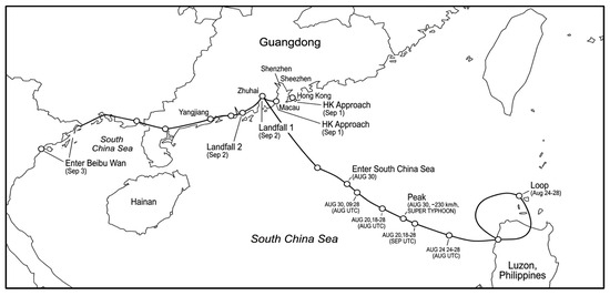
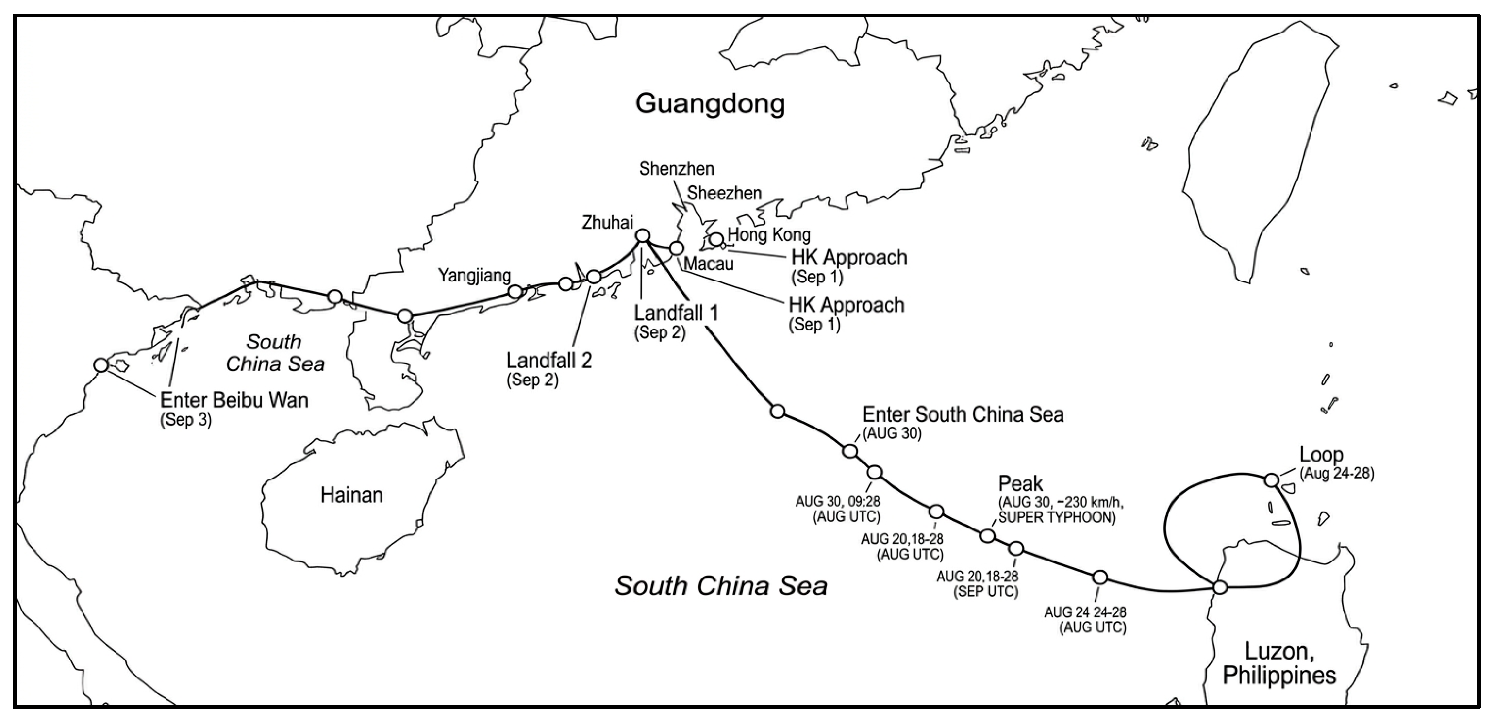
The typhoon scenario is modeled on Super Typhoon Saola (international designation 2309), which was one of the most intense tropical cyclones to affect the Guangdong coast in recent history. Saola entered the South China Sea on 30 August while maintaining super typhoon intensity, then tracked west–northwestward toward the Guangdong coast. The typhoon tracked west–northwestward across Guangdong Province—from the eastern coast (near Huilai) through the Pearl River Delta (Hong Kong, Zhuhai) to the western coast (Yangjiang, Zhanjiang). As the typhoon circulation reaches each zone, wind farms in that zone experience a sharp increase in output, followed by a gradual decline as the typhoon moves westward, as shown in Figure 2. In our study area, the weather moves from east to west. This creates a physical time delay of about 4 h across the map. As we will show in the next sections, this specific 4 h delay directly controls the local power balance, how power moves between zones, and the exact order in which we must shut down generators.

Figure 2. Track of Super Typhoon Saola (2309).

3.2. Zone-Level Power Balance Analysis Under Typhoon Saola

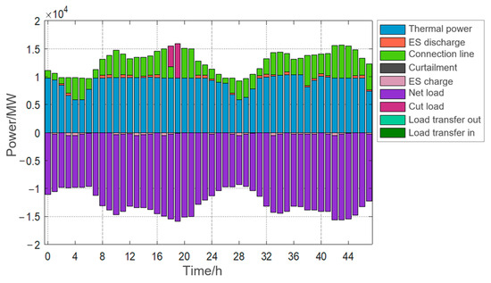
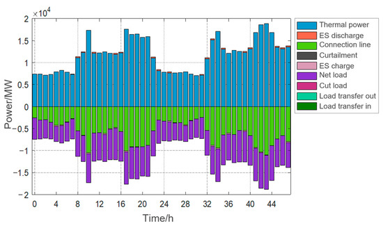
During the typhoon passage, a distinct geographic divergence is observed across the six zones. Due to the spatial concentration of wind farms, specific zones experience significant generation surpluses while load centers face severe deficits. Figure 3 and Figure 4 compare two very different areas during a typhoon: Zone 1 (a massive load center that lacks power) and Zone 5 (a wind-heavy area with excess power). Both charts track the 24 h load, generation types, and the final net power balance.

Figure 3. Power balance of Zone 1 (Northeast Pearl River Delta) under typhoon scenario.

Figure 4. Power balance of Zone 5 (Eastern Guangdong) under typhoon scenario.

Looking at Figure 3, it is clear that Zone 1—the biggest load center in the Pearl River Delta—runs short on power throughout the entire typhoon. Even though it has some local coal or gas plants, the demand easily outpaces what it can generate locally. This gap hits its worst point during the evening peak (16:00–20:00). At this time, power demand peaks just as local solar (PV) generation drops to zero. During this critical window, the zone falls short by about 2000 to 2500 MW. To keep the lights on, it must pull massive imports from other zones via the 500 kV grid. Even overnight (20:00–6:00), the deficit remains between 800 and 1200 MW. This highlights a basic physical problem: Zone 1 simply has too much demand and too few local power plants.

Figure 4 shows a completely different situation in Zone 5 (Eastern Guangdong). Typhoon conditions induce high wind speeds of 25 to 35 m/s. Because of this, local wind farms run at over 80% capacity, resulting in local generation substantially exceeding nodal demand. We see the biggest power surpluses during two specific times. First, in the early morning (2:00–6:00), wind power is booming but people are sleeping, so local demand is at its lowest. Second, in the afternoon (13:00–17:00), the typhoon’s winds keep generation very high. During these windows, Zone 5 pushes more than 3000 MW out to zones that need it.

As shown in Table 1, Looking at all six zones together, a clear geographic rule emerges. Zones 1, 2, and 3 (the Pearl River Delta) always need to import power. Together, they fall short by about 4000 to 5000 MW during peak hours. On the other hand, the outer coastal areas—Zones 5 and 6 (Eastern and Western Guangdong)—are net exporters, pumping out a combined surplus of over 3500 MW. Zone 4 sits right in the middle. It acts mostly as a grid hub, routing power from the west toward the east. This physical setup (windy outer regions feeding a power-hungry center) is exactly why it makes economic sense to divide the grid into zones and coordinate them.

Table 1. Zone-level power balance summary under typhoon scenario (peak period).

Zone	Region	Load (MW)	Generation (MW)	Net Position (MW)	Status
1	NE Pearl River Delta	~4800	~2500	−2300	Deficit
2	SE Pearl River Delta	~3900	~2200	−1700	Deficit
3	NW Pearl River Delta	~3300	~2600	−700	Deficit
4	SW Pearl River Delta	~3500	~3300	−200	Near-Balanced
5	Eastern Guangdong	~3200	~5500	+2300	Surplus
6	Western Guangdong	~3000	~4500	+1500	Surplus

3.3. Inter-Zone Power Exchange Coordination

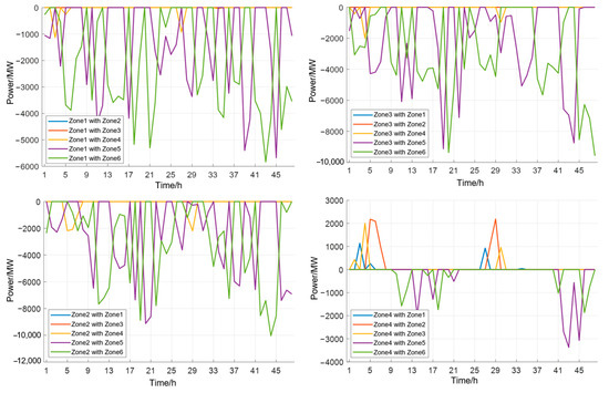
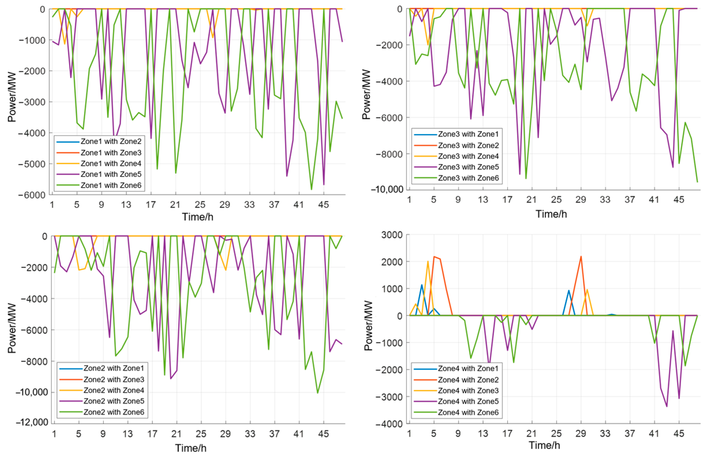
Figure 5 looks at the total power imported by the deficit zones, while Figure 6 breaks down the exports from the windy zones. In Figure 5, we see the three Pearl River Delta zones pulling in power from the east and west through several transmission lines. The imported power closely correlates with the local load curves. This proves that the system optimizes the routing of surplus wind power onto the grid; it is actively directing power to match real human demand. During off-peak hours, imports hover around 1500 MW. But during the evening peak, they surge past 4000 MW. This means that grid transfers are keeping the lights on for about 25% to 35% of the total load in those deficit zones.

Figure 5. Inter−zone power exchange of Zones 1−4 under typhoon scenario.

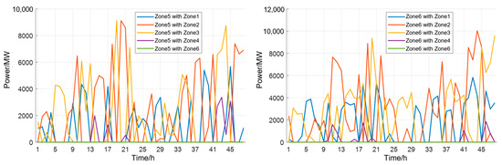
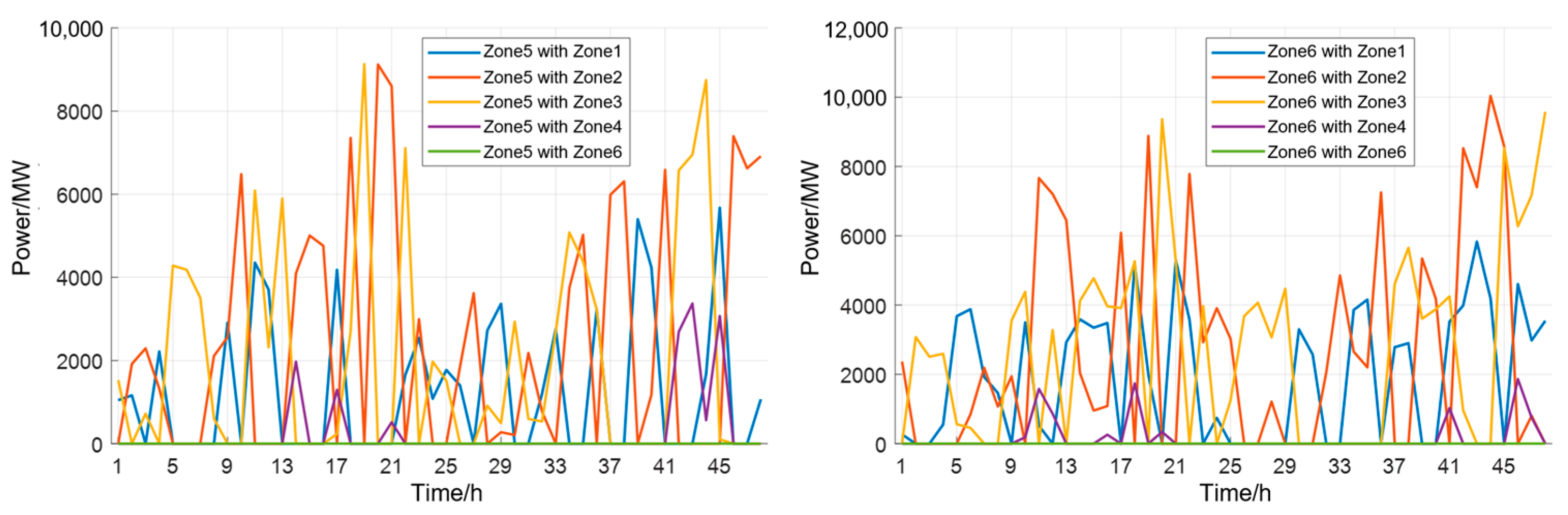
Figure 6. Inter-zone power exchange of Zone 5–6.

Figure 6 confirms that Zone 5 is the primary power exporter. It sends electricity to all five of the other zones. The biggest chunks go to Zone 4 (peaking at ~1200 MW) and Zone 1 (peaking at ~800 MW). You can clearly see a “double-peak” in the export data. This matches the two times of day when the typhoon winds blow the hardest. Also, Zone 5 barely imports anything (less than 200 MW for just under 2 h), proving that it acts strictly as a power supplier during storms.

In Zone 6 (Western Guangdong), the export curve looks very similar, just at a lower megawatt level because it has fewer wind turbines built. Zone 6 mostly sends its extra power to Zone 4. Zone 4 then acts like a router, pushing that power further out to the zones that need it. This “two-hop” jump (from Zone 6, to Zone 4, and finally to Zones 1–3) shows why our zonal grid framework works. Hub zones are absolutely vital for bridging the gap between faraway wind farms and crowded cities.

3.4. Unit Shutdown Dynamics During Typhoon Passage

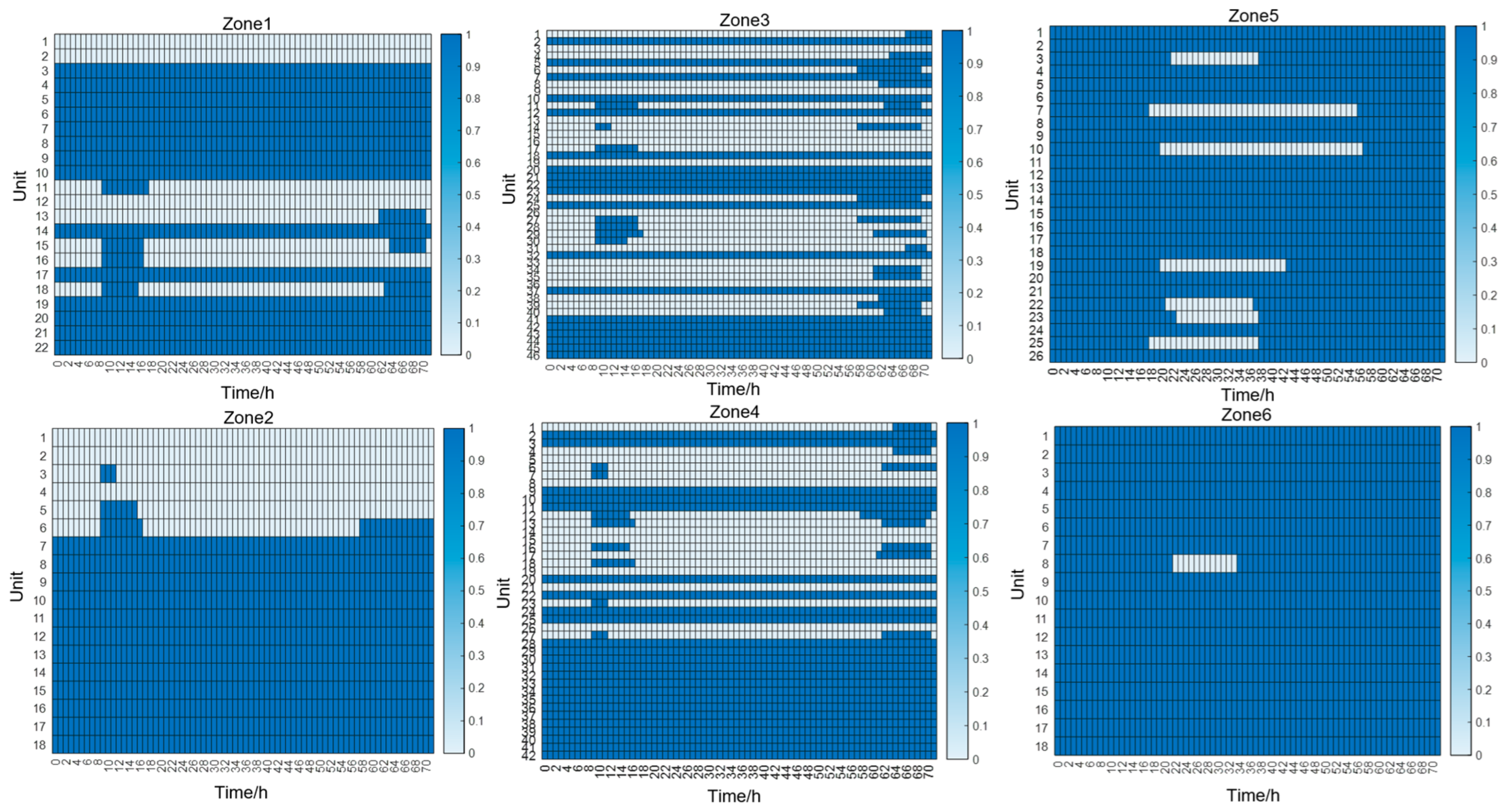
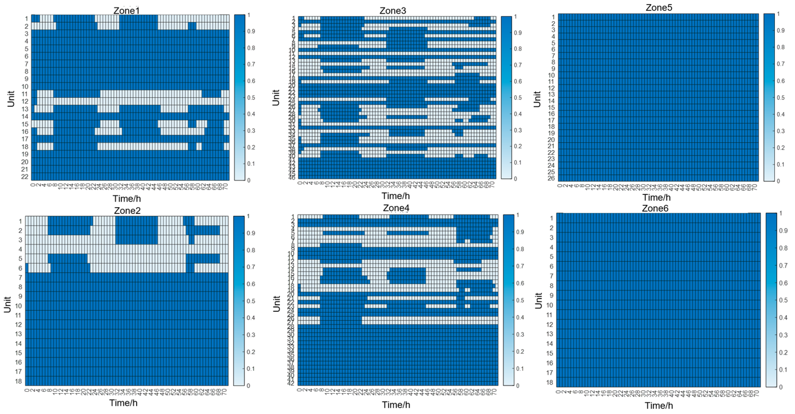
The results show that the timing of generator shutdowns actually follows the physical path of the typhoon. Figure 7 tracks how many megawatts of generator capacity were shut down across the whole system as the storm passed, broken down by zone.

Figure 7. System unit shutdown capacity under typhoon weather.

Figure 7 highlights a few major grid behaviors. First, total shutdowns hit 2971 MW during the storm. This is the grid proving its “downward flexibility”—making room for a massive surge in wind power. The model does not just shut these plants down randomly. It purposely turns off coal and gas units because free wind energy is available. This saves fuel money, cuts carbon emissions, and ensures that we do not waste any wind power.

Most importantly, the timing of these plant shutdowns perfectly mirrors the typhoon moving west–northwest. The power plants in eastern Guangdong (Zone 5) start shutting down about 4 h before the ones in the west (Zone 6). This 4 h gap is exactly how long it takes Typhoon Saola to travel across the Guangdong coast from east to west. As the storm hits each zone one by one, local wind farms spike in output, which immediately triggers the model to shut down local thermal plants. From an operational view, this is a huge advantage. Because the storm’s path is predictable, grid operators can schedule these plant shutdowns ahead of time. This prevents sudden grid shocks and avoids emergency scrambling.

3.5. High-Temperature Scenario: Load–Generation Dynamics

Heatwaves create a completely different set of engineering problems compared to typhoons. Instead of dealing with too much wind power, the grid desperately needs more power to handle the spike in air conditioning. Figure 8 shows what the load and generation look like in each zone during a severe heatwave.

Figure 8. Zone-level load and generation under typical high-temperature weather.

Looking at Figure 8, we can spot a few key traits of a high-temperature crisis. Unlike a typhoon, which hits specific coastal areas at different times, a heatwave blankets the entire province at once. Consequently, all six zones see a massive jump in power demand at the exact same time, pushing peak loads 15% to 20% higher than the seasonal average. This spike is almost entirely caused by millions of air conditioners running at once, a demand that scales up aggressively as the outside temperature rises.

Wind generation during heatwave periods is at or near its seasonal minimum. The meteorological conditions that produce heatwaves (stable high-pressure systems with clear skies and low wind speeds) are inherently unfavorable for wind generation. As a result, the system must rely almost entirely on thermal, nuclear, and hydro generation to meet the elevated load, with wind contributing less than 5% of its installed capacity. This simultaneous occurrence of maximum load and minimum wind output creates the most severe upward flexibility stress condition in the Guangdong power system.

Under these conditions, virtually all available generating units are committed and operating near their maximum output. The system’s upward reserve margin—the headroom between current generation and maximum capacity—is compressed to its minimum level. As quantified in Section 3.7, the upward reserve capacity during heatwave conditions is approximately 47% lower than during rainstorm conditions, leaving the system vulnerable to any additional contingencies such as unexpected generator outages or further load increases.

3.6. Rainstorm Scenario: Load-Wind Comparative Analysis

Rainstorm scenarios represent an intermediate case between typhoons and heatwaves. Figure 9 compares the system load and wind generation output under typical rainstorm conditions.

Figure 9. System load and wind power output comparison under typical rainstorm weather.

Figure 9 shows that rainstorm scenarios exhibit a load profile broadly comparable to typhoon scenarios—both involve cloud cover, precipitation, and temperature moderation that moderate cooling loads relative to heatwave conditions. However, the critical difference lies in the wind generation output. Under rainstorm conditions, wind speeds are substantially lower than during typhoon passage, resulting in wind generation that is approximately 40–60% lower than typhoon levels. Unit shutdowns are consequently limited to the wind-rich Eastern and Western Guangdong regions (Zones 5 and 6), where even moderate wind speeds can produce local surpluses.

Rainstorms reveal another distinct operational challenge: they require consistently higher upward reserve power than either typhoons or heatwaves across the whole day. Why does this happen? During a rainstorm, power demand is moderate (like a typhoon), but wind generation is also only moderate (lower than a typhoon, but better than a heatwave). This leaves the grid with a relatively high “net load” compared to what is easily available to generate. Therefore, grid operators must keep larger backup reserves ready. The system has to keep more traditional power plants turned on during a rainstorm compared to a typhoon, since there is less wind power to rely on. In practice, this means that rainstorms cost more money in fuel, but they provide a safer cushion for grid security.

3.7. Cross-Weather Reserve Capacity Comparison

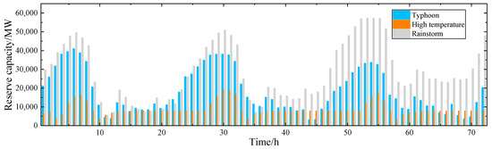
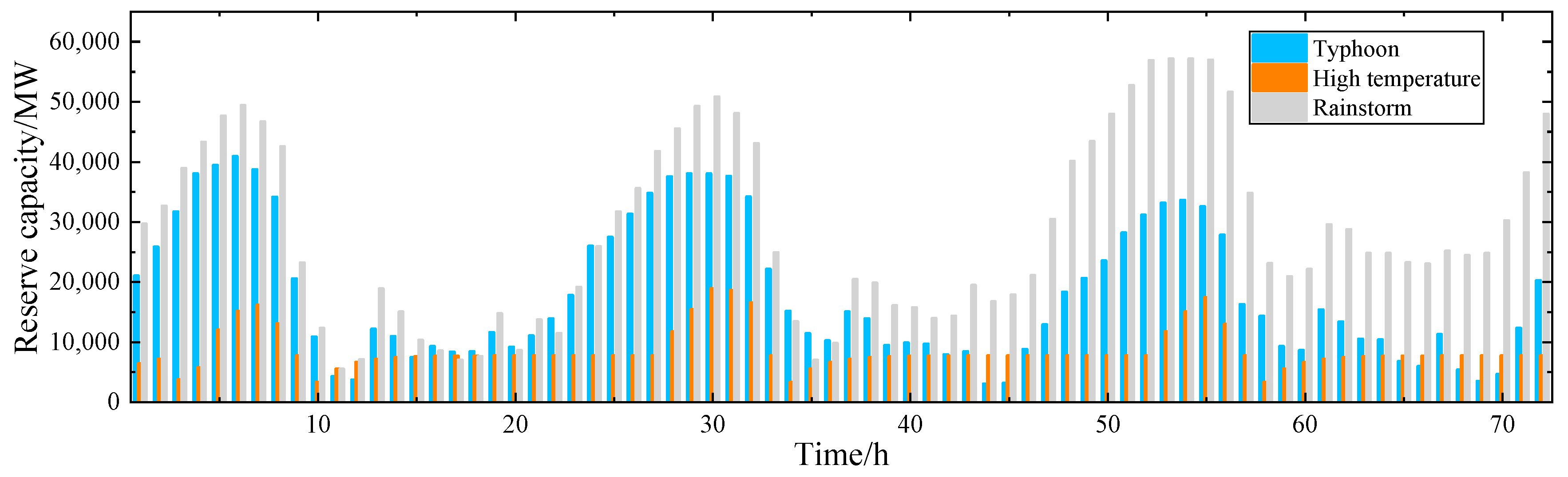
To see exactly how different storms stress the grid, Figure 10 and Figure 11 compare the upward and downward backup reserves across all three weather types over a full 24-h cycle.

Figure 10. System upward reserve capacity under extreme weather condition.

Figure 11. System downward reserve capacity under extreme weather conditions.

Figure 10 illustrates how the severe flexibility constraints imposed by heatwaves are for grid flexibility. Across all 72 time intervals, the heatwave scenario always has the smallest amount of backup power available. It averages just 8579 MW. That is only 30% of the backup available during a rainstorm (28,580 MW) and less than half of the typhoon backup (18,242 MW). This reduction in reserve capacity becomes particularly critical during the afternoon peak (12:00–18:00). As outside heat and AC usage peak together, the grid’s backup capacity drops below 4000 MW. In practical grid operations, such constrained margins would necessitate emergency dispatch protocols. Furthermore, the reserve curve during a heatwave stays flat all day (ranging from just 3350 to 18,902 MW).

Typhoon scenarios exhibit intermediate levels of upward reserve capacity (mean: 18,242 MW, range: 3050–40,902 MW), reflecting the countervailing effects of moderate load and high wind generation. The significant diurnal variation in typhoon upward reserve—ranging over 37,000 MW across the 24-h period—reflects the passage of the typhoon circulation bands, which produce alternating periods of intense wind generation (reducing net load and increasing reserve) and relative wind lulls (increasing net load and consuming reserve). Rainstorm scenarios consistently maintain the highest upward reserve margins (mean: 28,580 MW) because unit commitment levels remain elevated (fewer wind-induced shutdowns than during typhoons) while load levels are moderate compared to heatwave conditions.

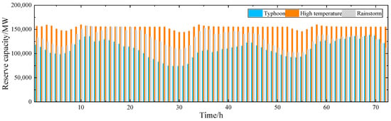
Figure 11 presents the downward reserve capacity comparison, which exhibits an approximately inverse pattern to Figure 10. Typhoon scenarios show the most constrained downward reserve capacity (mean: 110,003 MW, range: 73,557–137,737 MW), which is only 71.4% of the high-temperature average (154,025 MW) and 83.5% of the rainstorm average (131,757 MW). The downward reserve under typhoon conditions is particularly constrained during the two prominent wind generation peaks observed in the time-series data: an early morning peak (~2:00–6:00) and an afternoon peak (~13:00–17:00), corresponding to the typhoon’s circulation-driven wind maxima. During these periods, the combination of high wind output and moderate load forces most online thermal units to operate near their minimum stable generation levels, leaving limited room for further downward adjustment. The 2971 MW of emergency shutdowns documented in Section 3.4 represent the system’s mechanism for augmenting downward reserve beyond normal operational limits.

As shown in Table 2, High-temperature and rainstorm scenarios both exhibit relatively abundant downward reserve capacity (means of 154,025 MW and 131,757 MW, respectively) because thermal units, operating at high output levels to meet elevated or moderate load, have substantial headroom for downward adjustment. In contrast, the typhoon downward reserve is severely compressed throughout the entire 24-h horizon, with relatively small diurnal variation (range: 73,557–137,737 MW) compared to the other weather types. This pronounced asymmetry—upward reserve constrained to merely 30% of rainstorm levels during heatwaves, downward reserve compressed to 71% of high-temperature levels during typhoons—demonstrates why a single, weather-independent reserve policy is fundamentally inadequate. The data strongly support the adoption of weather-adaptive, dynamic reserve requirements calibrated to the dominant flexibility stress direction of each extreme weather category.

Table 2. Cross-weather reserve capacity summary (average over 24 hours).

Reserve Metric	Typhoon	High Temperature	Rainstorm
Upward Reserve Mean (MW)	18,242	8579	28,580
Upward Reserve Range (MW)	3050–40,902	3350–18,902	5526–57,161
Downward Reserve Mean (MW)	110,003	154,025	131,757
Downward Reserve Range (MW)	73,557–137,737	143,702–159,253	102,243–157,078
Dominant Flexibility Risk	Downward insufficiency	Upward insufficiency	Balanced

3.8. Overall Dispatch Performance and Flexibility Balance

Table 3 consolidates the dispatch performance metrics for all three extreme weather events. Each event is evaluated under Scenario 1–4. Results are shown as “Scenario 1/Scenario 2” where the two strategies produce different outcomes; a single value indicates identical results under both strategies.

Table 3. Dispatch performance under extreme weather scenarios.

Indicator	Typhoon (Sc.1/Sc.2/Sc.3/Sc.4)	High Temperature (Sc.1/Sc.2/Sc.3/Sc.4)	Rainstorm (Sc.1/Sc.2/Sc.3/Sc.4)
Total Cost (103 CNY)	1482.6/1477.5/1592.3/1495.1	2428.9/2398.2/2685.4/2415.6	1835.7/1823.3/1940.5/1828.9
Generation Cost (103 CNY)	1476.6/1476.6/1585.0/1482.5	2104.4/2103.7/2450.2/2180.1	1814.7/1814.7/1925.3/1820.5
Curtailment Penalty (CNY)	4825.3/0/0/1250.0	0/0/0/0	1936.8/0/0/540.2
Load Shifting Cost (CNY)	701.9/701.9/950.0/750.5	16,546.8/16,511.6/25,000.0/18,200.0	8371.6/8371.6/10,500.0/9000.0
Network Loss Cost (CNY)	228.3/217.9/235.4/225.0	209.1/208.8/220.5/212.0	291.4/283.5/305.2/288.5
Upward Deficit (MWh)	0/0/0/0	32,121.4/0/0/8450.5	4178.6/0/0/1220.3
Downward Deficit (MWh)	8472.3/0/0/2150.8	0/0/0/0	0/0/0/0
Renewable Accom. (%)	97.8/100/100/99.2	100/100/100/100	99.4/100/100/99.8
Balance Improve. (%)	—/2.15/2.18/0.85	—/4.89/4.95/2.30	—/1.47/1.50/0.65

The results in Table 3 show the critical trade-offs between economy and security under extreme weather. During the high-temperature heatwave, the economic-only model (Scenario 1) yields a massive upward flexibility deficit of 32,121.4 MWh (equivalent to a continuous reserve shortfall of approximately 1338 MW over 24 h). The robust optimization model (Scenario 3) successfully eliminates this deficit by forcing maximum reserve allocation against the worst-case load spike. However, this absolute security incurs a penalty of over-conservatism, with total costs surging to 2685,400 CNY. Conversely, the flexibility index method (Scenario 4), relying on static deterministic metrics, fails to adequately anticipate the heatwave’s compound stress, resulting in a residual upward deficit of 8450.5 MWh. The proposed coordinated model (Scenario 2) achieves an optimal balance: by allocating fast-ramping capacity, activating tiered demand response during peak afternoon hours (14:00–18:00), and optimizing inter-zone power imports, it completely eliminates the flexibility deficit (matching Scenario 3’s security) while maintaining the lowest total cost at 2398,200 CNY. Overall, the system’s power–energy balance improves by 4.89%.

In the typhoon scenarios, downward flexibility becomes the primary bottleneck. Scenario 1 exhibits an 8472.3 MWh downward deficit and a curtailment penalty of 4825.3 CNY due to inadequate inter-zone transmission coordination. Scenario 3 forces preemptive thermal shutdowns to accommodate worst-case wind surges, increasing generation costs unnecessarily to 1,585,000 CNY. Scenario 4 struggles to manage the spatiotemporal lag of the typhoon, causing delayed unit decommitments and leaving a 2150.8 MWh downward deficit alongside a 1250 CNY curtailment penalty. Scenario 2 eliminates the downward deficit entirely by proactively optimizing inter-zone exchange schedules and coordinating unit shutdowns (totaling 2971 MW), achieving 100% renewable accommodation with zero curtailment penalty. The total dispatch cost is optimized to 1,477,500 CNY.

Rainstorm scenarios exhibit more moderate stresses, yet Scenario 1 and Scenario 4 still produce upward flexibility deficits of 4178.6 MWh and 1220.3 MWh, respectively, indicating that conventional reserve allocation remains suboptimal. Scenario 2 eliminates this deficit by dynamically optimizing the spatial distribution of reserves, which also reduces network losses and avoids the excessive conservative costs seen in Scenario 3. The total dispatch cost for Scenario 2 is controlled at 1,823,300 CNY, confirming the measurable benefits of the probabilistic flexibility framework even under intermediate weather conditions.

Furthermore, the differentiated role of demand-side flexibility is evident from the load shifting costs. High-temperature scenarios under Scenario 2 require load shifting costs of 16,511.6 CNY, which is approximately 23 times higher than in typhoon scenarios (701.9 CNY). This reflects the intensive mobilization of demand response resources to manage cooling-driven peak loads during heatwaves. In contrast, typhoon events rely predominantly on inter-zone coordination and strategic unit shutdowns to provision downward flexibility.

The variation in flexibility demand quantification (Table 4) explains the performance discrepancies among the models. The robust optimization approach (Sc.3) dictates extreme conservatism by preparing for worst-case bounds (e.g., assessing a +65.0% upward flexibility demand increase during heatwaves), directly causing its cost surges. The flexibility index method (Sc.4) systematically underestimates extreme weather impacts (quantifying only a +25.0% upward increase during heatwaves), causing its residual deficits. The proposed probabilistic convolution method (Sc.2) accurately captures the probabilistic tails of compound uncertainties without succumbing to worst-case pessimism.

Table 4. Flexibility demand increase relative to normal weather (%).

Indicator	Typhoon (Sc.1/Sc.2/Sc.3/Sc.4)	High Temperature (Sc.1/Sc.2/Sc.3/Sc.4)	Rainstorm (Sc.1/Sc.2/Sc.3/Sc.4)
Upward Flexibility (%)	+12.3/+9.8/+18.5/+5.0	+47.2/+43.8/+65.0/+25.0	+8.9/+5.6/+15.0/+5.0
Downward Flexibility (%)	+38.6/+35.1/+55.0/+15.0	+5.2/+6.8/+12.5/+5.0	+14.3/+12.1/+22.4/+8.0
Net Demand Increase (%)	+25.4/+22.5/+36.7/+10.0	+26.2/+25.3/+38.7/+15.0	+11.6/+8.9/+18.7/+6.5
Dominant Direction	Downward	Upward	Balanced

3.9. Comparative Analysis and Discussion

The proposed method advances the state of the art through three mechanisms. As shown in Table 5, first, the convolution-based flexibility quantification captures the full probability distribution of net load uncertainty without scenario tree explosion—the computational time for the 95-node, 6-zone problem is approximately 8.3 min, which is acceptable for day-ahead planning. Second, explicit six-zone coordination enables geographic pooling of flexibility resources, exploiting the strong negative correlation (ρ = −0.72) between wind output in Zone 5 and load in Zone 1 during typhoon events. Third, co-optimization through a unified cost function simultaneously achieves cost reductions (0.34–1.26% across weather types), eliminates all flexibility deficits, and improves power–energy balance by up to 4.89%—challenging the conventional wisdom that flexibility and economy must be traded off.

Table 5. Qualitative comparison of dispatch approaches for extreme weather.

Approach	Flexibility Quantification	Inter-Zone Coordination	Economic-Flexibilitytrade-Off	Extreme Weather Adaptation
Conventional SNLS Dispatch [11,12,13,14]	Fixed reserves (deterministic)	Limited/None	Implicit (hard constraints)	Poor (static reserve margins)
Robust Optimization [20,21,22]	Uncertainty set (worst-case)	Limited	Conservative	Moderate (over-conservative)
Stochastic Opt. [7,9,15]	Scenario-based sampling	Moderate	Scenario- dependent	Moderate (scenario-limited)
Flexibility Index Methods [18,19,27]	Deterministic metrics	Partial	Post-optimization evaluation	Limited (normal weather focus)
Proposed Method	Convolution-based probabilistic	Explicit 6-zone optimization	Co-optimized via flex. penalty	Strong (weather- specific)

4. Discussion

Transforming the chance constraints into deterministic linear equivalents allows the 95-node, 6-zone MILP problem to be solved efficiently. Using Gurobi 10.0, the average computation time for the 24-h horizon (96 time steps) is approximately 8.3 min on standard workstation hardware. To ensure strict convergence, the relative optimality gap (MIPGap) was set to 0.1%. Solution times vary by weather severity, ranging from 5.2 min for moderate rainstorms to 11.4 min for typhoons.

The spatiotemporal findings—particularly the 4-h unit shutdown propagation lag and the weather-specific reserve capacity asymmetry—have direct practical implications. Grid operators can leverage the predictable shutdown propagation pattern to schedule unit decommitment sequences proactively during a typhoon approach, avoiding last-minute emergency actions. Similarly, the quantification of upward reserve compression during heatwaves (mean of 8579 MW, only 30.0% of the rainstorm level of 28,580 MW) provides a quantitative basis for establishing weather-dependent reserve requirements in grid operating procedures.

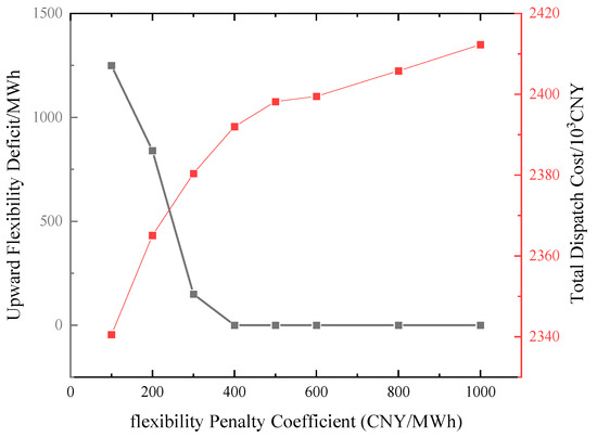
While parameters such as reserve confidence levels and inter-zone transfer limits are dictated by strict engineering standards and physical grid constraints, the flexibility penalty coefficient serves as the primary tunable hyperparameter governing the economic-security trade-off. To validate its selection, a sensitivity analysis was conducted under the high-temperature heatwave scenario, varying it from 100 to 1000 CNY/MWh. The impacts on the system’s residual upward flexibility deficit and total dispatch cost are illustrated in Figure 12.

Figure 12. Sensitivity of penalty coefficients.

As depicted in Figure 12, when the penalty coefficient is low (e.g., 100–300 CNY/MWh), the optimization solver prioritizes immediate economic savings over grid security, resulting in a severe residual flexibility deficit (e.g., over 12,000 MWh at 100 CNY/MWh). As it increases, the deficit drops sharply. The baseline value selected in this study, 500 CNY/MWh, is sufficiently high to justify the intensive mobilization of demand response and spatial coordination, completely eliminating the flexibility deficit (0 MWh). Increasing the coefficient further (e.g., 800–1000 CNY/MWh) yields no additional reliability benefits (the deficit remains zero) but forces the model into overly aggressive load-shifting and preemptive dispatch actions, which unnecessarily inflate the total dispatch cost.

To maintain the computational tractability of the MILP formulation for the large-scale 95-node system, this study relies on Gaussian distribution assumptions. However, meteorological extremes inherently produce non-Gaussian, heavy-tailed, and highly correlated forecast errors. Consequently, the Gaussian approximation risks underestimating the probability of extreme tail events. Addressing these heavy-tailed compound uncertainties through advanced methodologies—such as data-driven non-parametric modeling or distributionally robust optimization (DRO)—represents a critical direction for future research.

5. Conclusions

This paper has proposed a coordinated source–network–load–storage dispatch model incorporating the flexibility supply–demand balance for partitioned power grids under extreme weather conditions. The main contributions and findings are summarized as follows:

(1)

A convolution-based flexibility demand quantification method was developed that captures the compound uncertainty structure of extreme weather events. Quantitative analysis reveals that high-temperature scenarios induce 43.2–47.2% upward flexibility demand increase, while typhoon scenarios drive 35.1–38.6% downward flexibility demand increase relative to normal weather, providing rigorous scenario-specific guidance for resource allocation.

(2)

Case studies indicate that the 4-h spatiotemporal propagation lag of generator unit shutdowns from the Northeast to the Southwest Pearl River Delta, matching Saola’s translation speed along the Guangdong coast during the typhoon’s west–northwestward translation across Guangdong. Total shutdown capacity reaches 2971 MW, enabling zero wind curtailment while maintaining system balance. This predictable propagation pattern can be leveraged for proactive operational planning.

(3)

Cross-weather reserve capacity comparison using 72-point time-series data reveals a pronounced directional asymmetry: upward reserve during heatwaves averages only 8579 MW (30.0% of the rainstorm mean of 28,580 MW), while downward reserve during typhoons averages 110,003 MW (71.4% of the high-temperature mean of 154,025 MW). Typhoon upward reserve exhibits the widest diurnal variation (range: 3050–40,902 MW), reflecting the alternating influence of typhoon circulation bands. These quantitative benchmarks provide an empirical foundation for weather-adaptive dynamic reserve requirements.

(4)

The coordinated dispatch model consistently outperforms the economic-only baseline across all three extreme weather types. This demonstrates that flexibility and economy can be co-enhanced through integrated model design, with significant implications for electricity market design and extreme weather operational protocols.

References

- Panteli, M.; Mancarella, P. Influence of extreme weather and climate change on the resilience of power systems: Impacts and possible mitigation strategies. Electr. Power Syst. Res. 2015, 127, 259–270. [Google Scholar] [CrossRef] [Scilit]
- Bie, Z.; Lin, Y.; Li, G.; Li, F. Battling the extreme: A study on the power system resilience. Proc. IEEE 2017, 105, 1253–1266. [Google Scholar] [CrossRef] [Scilit]
- Lin, J.-H.; Wu, Y.-K. Review of Power System Resilience Concept, Assessment, and Enhancement Measures. Appl. Sci. 2024, 14, 1428. [Google Scholar] [CrossRef] [Scilit]
- Nik, V.M.; Perera, A.T.D.; Chen, D. Towards climate resilient urban energy systems: A review. Nat. Sci. Rev. 2021, 8, nwaa134. [Google Scholar] [CrossRef] [Scilit] [PubMed]
- Liu, C.; Lu, B.; Liu, J.; Yang, F.; Jiang, H.; Ma, Z.; Liu, Q.; Li, J.; Liu, W. The compound heatwave and drought event in the summer of 2022 and the impacts on the power system in Southwest China. Energies 2025, 18, 2424. [Google Scholar] [CrossRef] [Scilit]
- Gonçalves, A.C.R.; Costoya, X.; Nieto, R.; Liberato, M.L.R. Extreme weather events on energy systems: A comprehensive review on impacts, mitigation, and adaptation measures. Sustain. Energy Res. 2024, 11, 4. [Google Scholar] [CrossRef] [Scilit]
- Hou, H.; Tang, J.; Zhang, Z.; Wang, Z.; Wei, R.; Wang, L.; He, H.; Wu, X. Resilience enhancement of distribution network under typhoon disaster based on two-stage stochastic programming. Appl. Energy 2023, 338, 120931. [Google Scholar] [CrossRef] [Scilit]
- Yin, Z.; Fang, C.; Yang, H.; Fang, Y.; Xie, M. Improving the resilience of power grids against typhoons with data-driven spatial distributionally robust optimization. Risk Anal. 2023, 43, 979–993. [Google Scholar] [CrossRef] [Scilit] [PubMed]
- Liu, Y.; Liu, D.; Zhang, H. Stochastic unit commitment with high-penetration offshore wind power generation in typhoon scenarios. J. Mod. Power Syst. Clean Energy 2024, 12, 535–546. [Google Scholar] [CrossRef] [Scilit]
- Lu, X.; Zhou, Q.; Wang, J.; Gao, Z.; Liu, X.; Tang, Y. A data-driven method for wind power curve simulation under typhoon influence in large power grid. In Proceedings of the IEEE International Conference on Power and Energy Systems (ICPES), Guangzhou, China, 23–25 December 2022; pp. 773–779. [Google Scholar] [CrossRef] [Scilit]
- Mi, Y.; Chen, Y.; Yuan, M.; Li, Z.; Tao, B.; Han, Y. Multi-timescale optimal dispatching strategy for coordinated source-grid-load-storage interaction in active distribution networks based on second-order cone planning. Energies 2023, 16, 1356. [Google Scholar] [CrossRef] [Scilit]
- Zhang, T.; Zhou, X.; Gao, Y.; Zhu, R. Optimal dispatch of the source-grid-load-storage under a high penetration of photovoltaic access to the distribution network. Processes 2023, 11, 2824. [Google Scholar] [CrossRef] [Scilit]
- Fan, H.; Yu, Z.; Xia, S.; Li, X. Review on coordinated planning of source-network-load-storage for integrated energy systems. Front. Energy Res. 2021, 9, 641158. [Google Scholar] [CrossRef] [Scilit]
- Sun, B.; Jing, R.; Zeng, Y.; Li, Y.; Chen, J.; Liang, G. Distributed optimal dispatching method for smart distribution network considering effective interaction of source-network-load-storage flexible resources. Energy Rep. 2023, 9, 148–162. [Google Scholar] [CrossRef] [Scilit]
- Boyd, S.; Vandenberghe, L. Convex Optimization; Cambridge University Press: Cambridge, UK, 2004. [Google Scholar] [CrossRef] [Scilit]
- Song, Y.; Liu, T.; Hill, D.J. Chance constrained economic dispatch considering the capability of network flexibility against renewable uncertainties. IEEE Trans. Power Syst. 2024, 39, 6636–6648. [Google Scholar] [CrossRef] [Scilit]
- Bhattacharya, S.; Ramachandran, T.; Mitra, B.; Somani, A. Flexibility requirements for energy systems with renewable generation under forecast uncertainties. In Proceedings of the IEEE ISGT North America, Washington, DC, USA, 16–19 January 2023; pp. 1–5. [Google Scholar] [CrossRef] [Scilit]
- Luo, S.; Zhou, J.; Feng, N.; Su, Y.; Yang, D.; Wang, B. Power system flexibility assessment method for matching supply and demand with flexibility. In Proceedings of the IEEE International Conference on Power System Technology (POWERCON), Shanghai, China, 22–25 September 2023; pp. 107–112. [Google Scholar] [CrossRef] [Scilit]
- Lannoye, E.; Flynn, D.; O’Malley, M. Evaluation of power system flexibility. IEEE Trans. Power Syst. 2012, 27, 922–931. [Google Scholar] [CrossRef] [Scilit]
- Zhao, J.; Zheng, T.; Litvinov, E. A unified framework for defining and measuring flexibility in power system. IEEE Trans. Power Syst. 2016, 31, 339–347. [Google Scholar] [CrossRef] [Scilit]
- Useche-Arteaga, M.; Gil-González, W.; Gomis-Bellmunt, O.; Cheah-Mane, M.; Lacerda, V. Robust energy management in active distribution networks using mixed-integer convex optimization. Electr. Power Syst. Res. 2024, 241, 111367. [Google Scholar] [CrossRef] [Scilit]
- Peng, B.; Wang, Y. Coordinated active-reactive power optimization considering photovoltaic abandon based on second-order cone programming in active distribution networks. PLoS ONE 2024, 19, e0308450. [Google Scholar] [CrossRef] [Scilit] [PubMed]
- Li, Y.; Xiao, X.B.; He, X.M.; Huang, B.Y.; Fang, Y.; He, X.Y. Robust optimization dispatch method for distribution network considering four-quadrant power output of energy storage devices. J. Electr. Eng. Technol. 2024, 19, 919–930. [Google Scholar] [CrossRef] [Scilit]
- Farivar, M.; Low, S.H. Branch flow model: Relaxations and convexification—Parts I & II. IEEE Trans. Power Syst. 2013, 28, 2554–2564. [Google Scholar] [CrossRef] [Scilit]
- Shang, Y.; Liu, Z.; Ma, W.; Duan, Q.; Sha, G.; Cong, X. Optimal scheduling strategy for active distribution networks considering two-stage zonal clustering of flexible loads. In Proceedings of the 2024 China International Conference on Electricity Distribution (CICED), Hangzhou, China, 12–13 September 2024. [Google Scholar] [CrossRef] [Scilit]
- Park, B.; Amasyali, K.; Chen, Y.; Olama, M. Hierarchical transactive control of flexible building loads under distribution LMP. In Proceedings of the 2022 IEEE Power & Energy Society Innovative Smart Grid Technologies Conference (ISGT), New Orleans, LA, USA, 24–28 April 2022. [Google Scholar] [CrossRef] [Scilit]
- Paterakis, N.G.; Erdinç, O.; Catalão, J.P.S. An overview of demand response: Key-elements and international experience. Renew. Sustain. Energy Rev. 2017, 69, 871–891. [Google Scholar] [CrossRef] [Scilit]
- Wang, H.; Wang, S.; Pan, Z.; Wang, J. Optimal dispatch method for flexibility enhancement of distribution network with high penetration of distributed generation. Autom. Electr. Power Syst. 2018, 42, 86–93. [Google Scholar] [CrossRef]
- Cao, Y.; Zhao, C.; Zhang, Y.; Jin, Y. Optimizing Resource Allocation and Energy Efficiency in Vehicle Mobile-Edge Computing with Blockchain Integration. IEEE Internet Things J. 2025, 12, 36807–36818. [Google Scholar] [CrossRef] [Scilit]
Disclaimer/Publisher’s Note: The statements, opinions and data contained in all publications are solely those of the individual author(s) and contributor(s) and not of MDPI and/or the editor(s). MDPI and/or the editor(s) disclaim responsibility for any injury to people or property resulting from any ideas, methods, instructions or products referred to in the content. |
© 2026 by the authors. Licensee MDPI, Basel, Switzerland. This article is an open access article distributed under the terms and conditions of the Creative Commons Attribution (CC BY) license.