


Abstract
A neural-network-assisted microwave-photonic method for interrogating fiber-optic sensing elements is proposed and numerically investigated. A multi-tone optical signal (MTOS), implemented as an optical frequency comb (OFC), is used to probe the spectral response of the sensing element. Square-law photodetection converts the interaction between the OFC lines and the sensing-element spectral response into beat components at difference frequencies, whose amplitudes form a multidimensional microwave-photonic response vector (MPRV). A unified numerical model based on transfer- and scattering-matrix formalisms was developed for fiber Bragg gratings (FBGs), Fabry–Pérot interferometers (FPIs), and combined FBG–FPI structures, including temperature-induced parameter variations and additive–multiplicative noise. A fully connected artificial neural network was trained to reconstruct the sensor state directly from the MPRV, with temperature used as the target measurand in the numerical study. It is shown that reconstruction accuracy is governed primarily by the distinguishability of sensor states in the MPRV space and by the practical one-to-one nature of the spectral position–MPRV mapping, rather than by neural-network complexity. Restricting the operating range to a practically one-to-one mapping region reduced the temperature reconstruction MAE from 0.198 to 0.021 °C at an SNR of 30 dB. Under increased noise, the proposed method exhibited slower accuracy degradation than spectral-peak, fixed-calibration, correlation-matching, and residual-minimization approaches, achieving the lowest MAE of 0.312 °C at an SNR of 15 dB. The method also demonstrated reduced sensitivity to OFC line-amplitude nonuniformity and residual optical-power drift. After training, the reconstruction time did not exceed 0.1 ms, indicating the potential of the proposed approach for high-speed fiber-optic sensor interrogation without direct optical-spectrum scanning.
1. Introduction
Fiber-optic measurement systems are widely used for monitoring temperature, strain, pressure, refractive index, and other physical quantities. Fiber Bragg gratings (FBGs) [1], Fabry–Pérot interferometers (FPIs) [2], and combined fiber-optic structures based on them [3] are commonly employed as sensing elements in such systems. In general, variations in the measurand lead to shifts and changes in the shape of their spectral response. Therefore, determination of the measured parameter requires acquisition of the spectral response of the sensing element and retrieval of the informative parameters that characterize this response.
Traditional interrogation methods based on optical spectrum acquisition using optical spectrum analyzers, tunable sources, spectral filters, or dispersive elements can provide high spectral resolution. However, increasing the resolution is generally accompanied by greater system complexity and cost and, in scanning systems, by reduced interrogation speed [4,5,6]. Additional limitations arise when the spectral features of sensing elements overlap, making individual spectral signatures difficult to distinguish [7,8,9]. Variations in optical power, operating-point drift, and the simultaneous influence of multiple physical quantities further reduce the robustness of simple calibration relationships [1]. Under these conditions, determining the spectral position of a sensing element from a single spectral feature or a fixed calibration relationship may no longer provide sufficiently robust measurement results.
High-speed interrogation techniques based on wavelength-to-time mapping and dispersive elements [10], mode-locked swept sources [11], or arrayed waveguide gratings [12] achieve excellent resolution and acquisition rates but rely on specialized optical components, precise synchronization, or are sensitive to environmental drift, necessitating dedicated compensation circuitry [13]. Microwave-photonic approaches based on chirped pulse compression [14], nonuniform microwave photonic filters [15], or integrated microring resonators [16] offer high speed and precision but often require complex radio-frequency signal synthesis or specialized nanofabrication.
A promising alternative to the mentioned approaches is microwave-photonic interrogation using a multi-tone optical signal (MTOS), which, in the implementation considered here, is generated as an optical frequency comb (OFC). The probing OFC consists of several discrete, equally spaced optical frequencies, the spacings between which belong to the radio-frequency range. When the discrete optical components of the comb interact with the spectral response of the sensing element, their amplitudes are modified according to the relative spectral alignment between the OFC and the sensing-element spectral response. The optical field consisting of lines with modified amplitudes is received by a photodetector, which generates the electrical signal proportional to the squared magnitude of the total optical field. The resulting electrical signal includes a DC term and cross-product (interference) terms between all possible pairs of optical lines. The set of their amplitudes forms a multidimensional microwave response. Unlike an individual amplitude component, this response vector characterizes the interaction of the OFC with the overall spectral response of the sensing element and therefore contains information about its spectral position.
The principle of microwave-photonic conversion, in which information on the spectral response of the sensing element is transferred to difference frequencies in the microwave domain, has been employed in a number of fiber-optic sensor interrogation systems [17,18,19]. The practical advantage of transferring spectral information to the microwave domain lies primarily in the simultaneous enhancement of interrogation speed, hardware simplicity, and measurement robustness. Traditional optical spectrum acquisition is fundamentally constrained by the scanning speeds of optomechanical components and the integration times required for high-resolution measurements. Microwave-photonic conversion overcomes this bottleneck by mapping the spectral interaction onto difference frequencies instantaneously and in parallel, enabling sub-millisecond data acquisition rates limited only by electronic processing speeds. Furthermore, the expensive, bulky optical spectrometers are replaced with relatively low-cost radio-frequency electronics for data extraction. This approach is particularly advantageous under conditions demanding high-speed dynamic monitoring, operation in noisy environments with significant optical power drift, and the interrogation of complex or overlapping spectral features where traditional single-peak tracking algorithms fail due to ambiguity.
In the proposed approach, the sensor state is represented by a multidimensional microwave-photonic response vector (MPRV) formed through the interaction of the optical frequency comb with the spectral response of the sensing element followed by photodetection. The MPRV components correspond to the amplitudes of signals at the difference frequencies and collectively encode information distributed across the microwave-photonic response of the sensing element. Thus, the MPRV defines the feature space used to solve the inverse interrogation problem.
The relationship between the spectral shift and the MPRV is nonlinear and is governed by the number and frequency spacing of the OFC lines, the spectral overlap between the OFC and the sensing-element spectral response, the shape of the sensing-element spectral response, the noise level, and the data normalization procedure. For symmetric relative alignments of the OFC and the sensing-element spectral response, different spectral positions of the sensing element may produce similar MPRVs, resulting in ambiguity in the inverse problem. Therefore, reconstruction of the spectral shift requires not only establishing an inverse mapping from the multidimensional response but also selecting an informative MPRV composition and an operating range within which the mapping between the spectral position and the MPRV remains one-to-one.
A multidimensional representation of the sensor state enables the joint use of information contained in multiple components of the measured response; however, increasing the number of features alone does not guarantee unambiguous reconstruction. A key requirement is identifiability: different sensor states must correspond to distinguishable response vectors within the selected operating range. If these vectors coincide or become indistinguishable in the presence of noise, the resulting ambiguity is inherent to the physical measurement process and cannot be eliminated by subsequent regression. Consequently, the formation of an informative feature space and the selection of an appropriate operating range should precede the optimization of the reconstruction algorithm.
Once sufficient distinguishability of the MPRVs has been ensured within the selected operating range, reconstruction of the sensor state reduces to the approximation of a multidimensional nonlinear mapping. Artificial neural networks (ANNs) [20,21] are well suited for approximating this multidimensional nonlinear relationship. Their use enables the spectral shift to be reconstructed directly from the set of beat-component amplitudes while accounting for the effects of noise and parametric perturbations.
The aim of this work is to develop and investigate a microwave-photonic interrogation method for fiber-optic sensors based on OFC probing and neural-network-assisted reconstruction of the sensor state from the MPRV, with temperature considered as the target measurand. The present study is a numerical proof-of-concept intended to establish the fundamental physical and algorithmic principles of the MPRV-based interrogation framework.
The combination of an FBG and an FPI is used as a composite fiber-optic sensor, which in some cases exhibits an asymmetric Fano resonance near the FBG central wavelength, thereby facilitating the enhancement of measurement resolution and sensitivity [22,23]. In addition, such combination of the sensing elements can enable simultaneous measurement of various physical quantities, e.g., temperature and refractive index [24], etc.
2. Materials and Methods
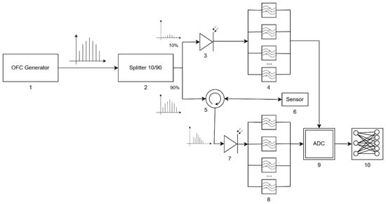
The structural diagram of the proposed microwave-photonic interrogation system is shown in Figure 1. In the implementation considered here, the probing MTOS is generated as an OFC consisting of M coherent spectral components with frequencies
where f0 is the reference optical frequency, Δf is the inter-line frequency spacing, and ak denotes the complex amplitude of the k-th spectral component. The optical field of the probing signal can then be represented as:
Figure 1.
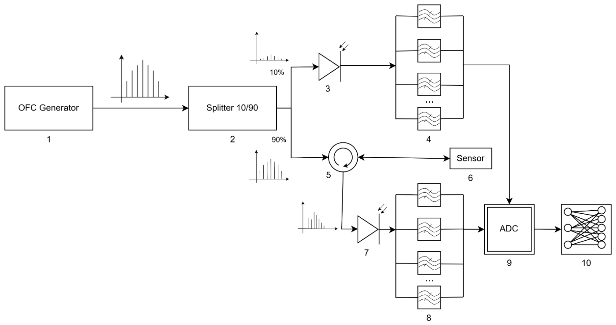
Structural diagram of microwave-photonic interrogation: 1—OFC generator; 2—optical power splitter; 3, 7—photodetectors; 4, 8—blocks for extracting beat components at difference frequencies; 5—optical circulator; 6—fiber-optic sensing element; 9—ADC; 10—software module for data normalization and neural-network processing.
The OFC generator 1 sets the number of spectral components, the inter-line frequency spacing, their amplitude distribution, and the shape of the overall spectral envelope. The generated probing signal is directed to the optical splitter 2, which divides it between the reference and measurement channels. In the measurement channel, the probing signal is routed through the optical circulator 5 to the sensing element 6.
The state of the sensing element is described by the complex spectral transfer function H(f, ξ), where ξ denotes the measured physical quantity or a related parameter that determines the spectral position of the response. For a reflective configuration, H(f, ξ) corresponds to the complex reflection coefficient, whereas for a transmissive configuration it corresponds to the complex transmission coefficient. Variations in temperature, strain, pressure, or another measured physical quantity lead to a shift in the spectral response of the sensing element and, in the general case, to a change in its shape.
After interaction of the probing OFC with the sensing element, the complex amplitude of the k-th spectral component is determined by the product of its initial complex amplitude and the value of the sensing-element spectral transfer function at the corresponding frequency, and can be written as:
and the output optical field is given by:
Thus, the spectral response of the sensing element performs amplitude-and-phase modulation of the probing OFC lines. Since the values of H(fk, ξ) are determined by the relative spectral alignment of the OFC lines and the sensing-element spectral response, its shift leads to a coordinated change in the set of complex amplitudes bk.
The radiation reflected from the sensing element is directed through the optical circulator to photodetector 7. Under square-law photodetection, the resulting measurement signal is proportional to the intensity of the total optical field:
For an equidistant OFC, the photocurrent contains a DC component I0(ξ) and beat components at the difference frequencies m·Δf, where m = 1,…, M − 1 [19,25,26,27]:
where the complex amplitude of the beat component at the m-th difference frequency is given by:
Therefore, each beat component is determined not by an individual OFC line but by the set of pairwise products of spectral components separated by the corresponding frequency interval. The amplitudes
characterize the relative spectral alignment between the OFC and the spectral response of the sensing element. Filter bank 8 extracts the beat components at the specified difference frequencies, after which their amplitudes are acquired by ADC 9.
In the reference channel, the radiation is directed directly to photodetector 3 and filter bank 4, bypassing the sensing element. As a result, a reference set of beat-component amplitudes Amref is formed, characterizing the initial OFC line-amplitude nonuniformity and the current state of the optoelectronic path. The normalized components of the measurement MPRV can be defined as:
This reduces the influence of source power variations, nonuniformity of the OFC spectral envelope, and slow drift in the transmission coefficients of individual components of the optoelectronic path. The reference channel and element-wise normalization are incorporated into the system architecture to increase the invariance of the input data to variations in the overall optical power level.
After filtering and normalization, the state of the sensing element is represented by the MPRV:
The MPRV therefore provides a physically formed multidimensional representation of the sensor state, in which information about the spectral response is distributed among several difference-frequency components. Its structure is determined jointly by the sensing-element response, the OFC parameters, and the microwave-photonic conversion process. The inverse interrogation problem can thus be formulated as reconstruction of the sensor state from this multidimensional representation.
The forward problem of microwave-photonic conversion is to determine the MPRV x for known parameters of the sensing element, the OFC, and the measurement path:
Its solution is used for system modeling and for generating labeled training data. The inverse problem is to reconstruct the spectral shift or directly the measured physical quantity from the acquired MPRV:
Since this mapping is nonlinear and depends on the shape of the sensing-element spectral response, the OFC parameters, the noise level, and the selected operating range, an artificial neural network is used to approximate it. The trained ANN implemented in software module 10 performs the regression mapping:
where θ denotes the set of neural-network weights and biases. Using the full MPRV makes it possible to account for the coordinated variation in multiple beat components, whereas an individual component does not, in general, provide an unambiguous determination of the spectral position of the sensing element.
3. Research Methodology
The spectral responses of the fiber-optic sensing elements were modeled within a one-dimensional transfer-matrix framework. For the FPI, a layered-medium model under normal incidence was employed, whereas the FBG was represented as a longitudinal periodic modulation of the effective refractive index of the guided mode. The parameters of each homogeneous layer were assumed to be constant across its thickness, while absorption and additional optical losses, when necessary, were taken into account by introducing a complex refractive index. The spectral responses of the FPI, FBG, and combined structure were calculated using transfer-matrix and scattering-matrix methods.
The FPI is represented as a sequence of two interfaces separated by a homogeneous optical cavity. The first interface corresponds to the “optical fiber–cavity” transition, whereas the second corresponds to the “cavity–output medium” transition. The overall transfer matrix of the FPI is determined as the product of the matrices of the individual elements in the order of optical propagation [2,28,29]:
where T12(n1, n2) and T23(n2, n3) are the transfer matrices of the interfaces between the first and second media and between the second and third media, respectively; T2(λ, n2, h) is the propagation matrix for the optical field inside the FPI cavity. The interface matrices are determined by the refractive indices ni of the adjacent media, whereas the cavity matrix is determined by its refractive index n2, geometric length h, and the optical wavelength λ.
The FBG is modeled as a one-dimensional periodic modulation of the effective refractive index of the optical fiber core. The transfer-matrix formalism is also used to calculate its spectral response, enabling the complex reflection and transmission coefficients to be determined as functions of the optical wavelength and grating parameters. The transfer matrix of a uniform FBG is written as [30]:
where λ is the optical wavelength; L is the FBG length; neff is the effective refractive index of the guided mode; Δn is the amplitude of the induced modulation of the effective refractive index; and Λ is the FBG period. The coupling coefficient κ, the detuning parameter Δβ, and the parameter γ are defined as follows:
The parameter Δβ characterizes the deviation in the probing wavelength from the Bragg resonance condition, whereas the coupling coefficient κ determines the strength of interaction between the counter-propagating modes. Variations in the grating period, effective refractive index, or amplitude of its induced modulation lead to changes in the position and shape of the FBG spectral response.
For modeling an apodized FBG, the grating was divided into MA locally uniform sections of length L/MA. Within each section, the parameters of the induced refractive-index modulation were assumed to be constant, and the overall transfer matrix of the apodized FBG was formed as the product of the matrices of the individual segments [30]:
where p is the apodization parameter, defined as the ratio of the amplitude of the induced refractive-index modulation at the FBG edges to its maximum value in the central region. This representation enables the spectral response of both uniform and apodized FBGs to be calculated within a unified matrix formalism.
For a combined sensing element comprising an FBG and an FPI connected in series, the overall transfer matrix of the structure is determined as the product of the matrices of the individual components in the order of their arrangement along the optical path:
where TFBG(λ, L, neff, Δn, Λ, MA) and TFP(λ, n1, n2, n3, h) are the transfer matrices of the FBG and FPI, respectively. This representation makes it possible to account for the combined effect of the spectrally selective reflection of the FBG and the interference properties of the FPI on the resulting spectral response of the sensing element. For a structure containing several spectrally selective elements arranged in series, the model is generalized by sequential multiplication of the corresponding transfer matrices.
The temperature effect on the fiber-optic sensing element was taken into account through the variation in its optical path length caused by the combined influence of the thermo-optic effect and thermal expansion [28]. In the linear approximation, for ΔT = T − T0, the temperature dependences of the sensing-element parameters were defined as:
where ΔT is the temperature change; ni,0 are the initial refractive indices; Kn,i, Kneff, and KΔn are the thermo-optic coefficients; αFP and αFBG are the thermal expansion coefficients of the FPI and FBG; and h0, L0, and Λ0 are the initial FPI cavity length, FBG length, and FBG period, respectively. The temperature-dependent parameters were substituted into the corresponding transfer matrices. Thus, the temperature effect was taken into account through variations in the physical parameters of the sensing element, followed by calculation of its spectral response.
To bring the simulated signals closer to the conditions of a real measurement path, both additive and multiplicative noise distortions were taken into account [7,8,31]. The additive component models disturbances whose amplitude does not directly depend on the useful-signal level, whereas the multiplicative component describes fluctuations that vary the signal amplitude in proportion to its instantaneous value. The noise sequences were generated using a generalized power-law model of the power spectral density:
where Sη(fη) is the noise power spectral density; fη is the noise frequency; C is a normalization coefficient; and β is the exponent that determines the spectral slope of the noise power density. In this study, particular attention was paid to pink noise, which is characterized by an increased power spectral density in the low-frequency range and by correlation between adjacent samples.
The generated noise sequences were normalized and scaled to the range [−1, 1]. The noisy signal was formed by simultaneously accounting for the additive and multiplicative noise components:
where s and sη are the original and noisy signals; ηM and ηA are the normalized realizations of multiplicative and additive noise; CM and CA are coefficients that determine the intensity of the corresponding noise components; n is the sample index; and ⮾ is the operation of element-wise multiplication of arrays. The combined additive–multiplicative noise model makes it possible to account simultaneously for both an independent noise background and distortions whose amplitude varies proportionally to the useful-signal level.
To determine the complex reflection and transmission coefficients, the resulting transfer matrix T(λ) is converted into the corresponding scattering matrix:
where F[⋅] denotes the transformation of the transfer matrix into the corresponding scattering matrix. The spectral reflection coefficient is determined as the squared magnitude of the S1,1 element of the scattering matrix:
For the reflective configuration, the complex spectral transfer function is H(λ, ξ) = S11(λ, ξ), whereas the power reflection coefficient is R(λ, ξ) = |H(λ, ξ)|2. The function H(λ, ξ) determines the changes in both the amplitudes and phases of the OFC lines resulting from their interaction with the sensing element.
When the temperature and/or another measured physical quantity changes, the parameters L, neff, Δn, Λ, n1, n2, n3, and h vary accordingly, resulting in a modification of the sensing-element spectral response and a corresponding change in the generated MPRV.
To solve the inverse problem of reconstructing the state of the sensing element, a fully connected feedforward ANN was used. The input to the ANN was the MPRV formed according to Equations (9) and (10), while the output was an estimate of the sensing element temperature T. Thus, neural-network training consisted in approximating the nonlinear mapping x(T) → T.
The training dataset was generated from numerical simulations of the MPRV while sequentially varying the temperature of the sensing element. In the case considered, the temperature was varied from 6 to 20 °C with a step of 0.01 °C. For each temperature value, the corresponding MPRV was calculated. To improve model robustness, additional signal realizations containing additive and multiplicative noise components were generated. As a result, the training dataset consisted of pairs of “MPRV–temperature” values.
The generated dataset was divided into training, validation, and test subsets in proportions of 70%, 15%, and 15%, respectively. To ensure reproducibility of the computational experiments, the random-number generator seed was fixed.
A fully connected feedforward neural network was used as the baseline architecture. Models with one to five hidden layers and with 12 to 256 neurons in each hidden layer were investigated. Based on the comparative analysis, an architecture comprising three hidden layers with 128 neurons in each layer was selected as the baseline model. The ReLU activation function was used in the hidden layers, whereas the output layer contained a single neuron with a linear activation function. The mean absolute error (MAE) was used as the loss function.
The network parameters were optimized using the Adam algorithm with an initial learning rate of 0.001, which was automatically reduced when no decrease in the validation error was observed. The mini-batch size was 64, and the maximum number of training epochs was 2000. To prevent overfitting, L2 regularization and early stopping were applied, with training terminated if the validation error did not decrease for 50 consecutive epochs. The investigated range of the L2 regularization coefficient was 10−5–10−3, while a value on the order of 10−4 was used for the baseline model.
For the baseline training dataset, the noise distortion level corresponded to a signal-to-noise ratio of approximately 30 dB. In the subsequent evaluation of noise robustness, signal-to-noise ratios of 40, 20, and 15 dB were additionally considered.
4. Numerical Modeling
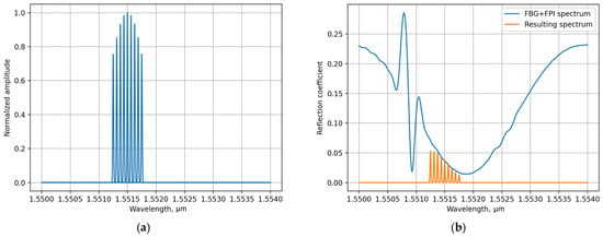
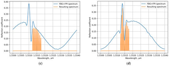
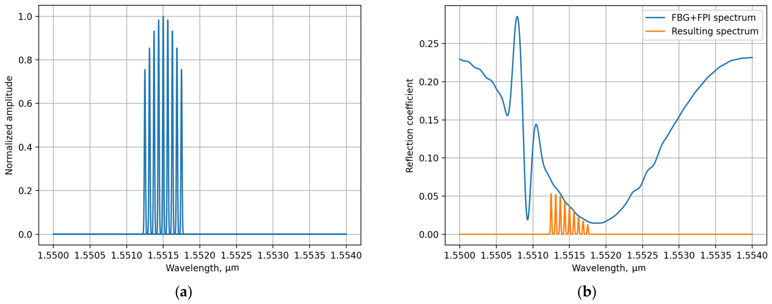
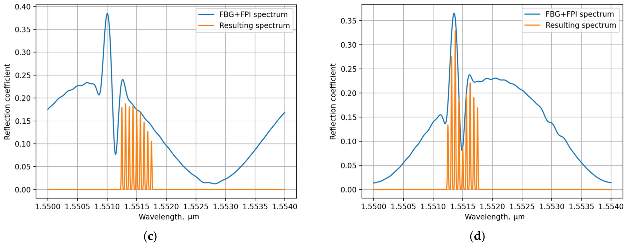
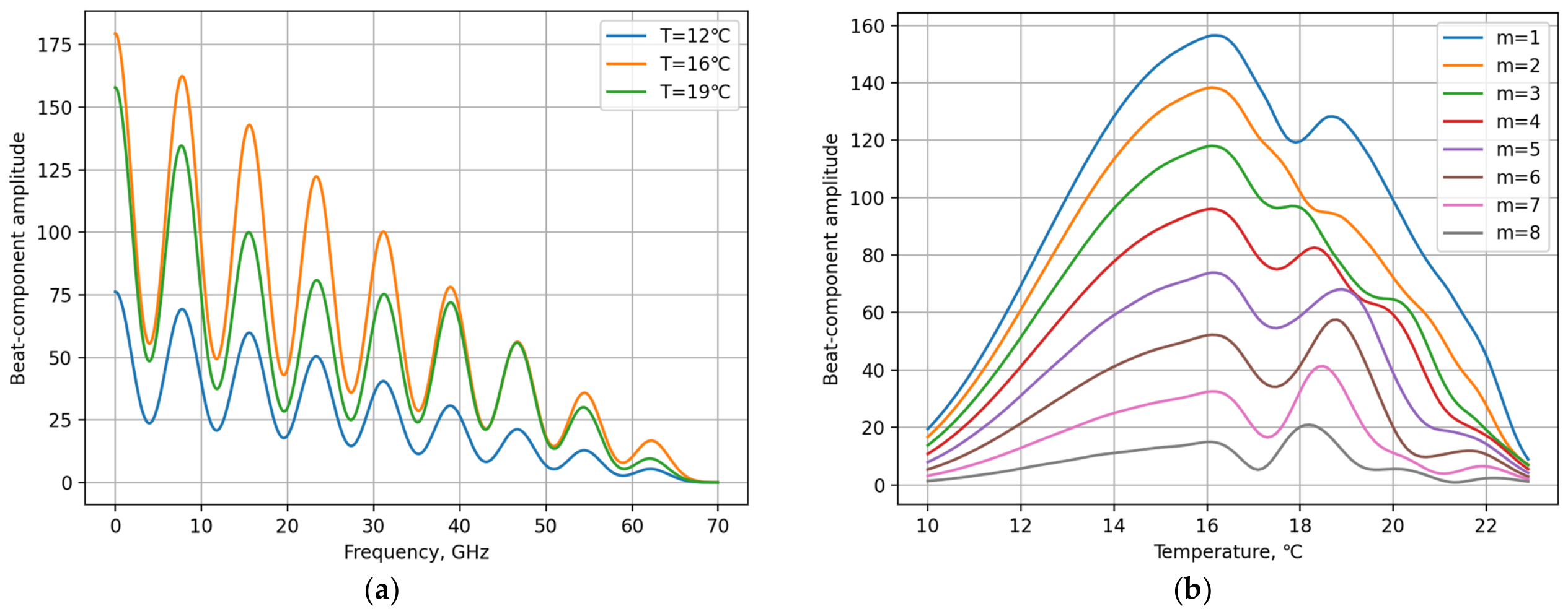
Numerical simulation of the microwave-photonic interrogation showed that the spectral shift of the sensing element is converted into a coordinated variation in the set of beat-component amplitudes at the OFC difference frequencies. The sequence of this conversion is illustrated in Figure 2. After interaction with the spectral response of the sensing element, the initial OFC (Figure 2a) acquires a nonuniform distribution of spectral-component amplitudes (Figure 2b–d), while photodetection produces a set of beat components at the difference frequencies (Figure 3a). When the spectral response shifts under temperature variation, the amplitudes of these components change, with both the magnitude and character of the variation differing from one component to another (Figure 3a,b).
Figure 2.
Optical spectra during microwave-photonic interrogation: (a) spectrum of the initial OFC; (b) spectrum after interaction with the sensing element at T = 12 °C; (c) spectrum after interaction with the sensing element at T = 16 °C; (d) spectrum after interaction with the sensing element at T = 19 °C.
Figure 3.
Electrical signal of the photodetector during microwave-photonic interrogation: (a) spectrum of the beat signal at various temperatures; (b) variation in the beat-component amplitudes at difference frequencies as the spectral response shifts under temperature variation.
This behavior highlights the advantage of representing the sensor state by a set of beat-component amplitudes rather than by a single amplitude feature. The value of an individual beat component reflects only one particular feature of the relative spectral alignment between the OFC lines and the sensing-element spectral response and, in the general case, does not provide an unambiguous determination of its spectral position. In contrast, the set of beat-component amplitudes forms a multidimensional representation of the sensing-element state in the form of an MPRV. Since individual MPRV components respond differently to the same spectral shift, their joint analysis contains substantially more information about the position of the spectral response than the analysis of a single beat component.
In the considered formulation, phase components were not included in the MPRV. Instead, the sensor state was represented using multiple amplitude features, which reduces sensitivity to fluctuations in optical path length and in the relative phases of the OFC spectral components.
Increasing the dimensionality of the input MPRV does not, by itself, guarantee a unique solution to the inverse problem. The determining condition is a one-to-one mapping between the spectral position of the sensing element and the resulting MPRV. The most significant violation of this condition occurs when the OFC lines and the sensing-element spectral response are symmetrically aligned. In particular, for an FBG, owing to the approximate symmetry of its reflection spectrum about the Bragg wavelength, spectral positions on opposite slopes of the reflection peak may produce similar MPRVs. In the vicinity of the spectral extremum, the sensitivity is further reduced because a small spectral shift produces only a slight change in the beat-component amplitudes.
The FBG simulation results directly demonstrate the nonmonotonic behavior of the MPRV as the spectral response passes through the region of symmetric alignment with the OFC and, consequently, the need to select the operating range on one of the slopes of the spectral response. Therefore, the operating range of the microwave-photonic system should be determined not only by the required range of variation in the measured physical quantity but also by the distinguishability of the MPRVs x(ξ), where ξ denotes the spectral shift or the corresponding measured physical quantity.
As the system approaches the region of symmetric alignment, this condition is violated in practical terms: the distance between MPRVs corresponding to different values of ξ becomes comparable to the vector variations caused by noise perturbations. Under these conditions, the neural network cannot eliminate the physical ambiguity inherent in the input data and is forced to approximate an averaged solution.
5. Results and Discussion
For quantitative evaluation, the neural-network model was investigated in the task of reconstructing the temperature of the sensing element. The execution and training of the ANN was performed using Python 3.11.3 (Wilmington, DE, USA) and TensorFlow 2.12.0 (London, UK) on a conventional PC based on the AMD Ryzen 7 7700 (Santa Clara, CA, USA) CPU. Numerical simulations were performed in the spectral region around 1552 nm. A combined structure was used as the sensing element, comprising an FBG with a central wavelength of 1552.15 nm, a length of L = 1 mm, and a refractive-index modulation amplitude of Δn = 10−5, together with an FPI having a cavity length of h = 10 μm and a refractive index of 1.5.
The probing OFC consisted of M = 9 equally spaced spectral components with an inter-line spacing of 7.81 GHz and a Gaussian spectral envelope. The FBG temperature was varied from 6 to 20 °C with a step of 0.01 °C. A combination of additive and multiplicative pink noise with β = 1 was used to model disturbances, with the noise sequences normalized to the range [−1, 1]. The baseline training dataset corresponded to a signal-to-noise ratio of approximately 30 dB, while the robustness of the method was additionally evaluated at signal-to-noise ratios of 40, 20, and 15 dB.
For the full investigated range at an SNR of 30 dB, the mean absolute error in temperature determination was 0.198 °C. As the regions associated with ambiguity were progressively excluded, the MAE decreased to 0.121, 0.076, 0.041, 0.027, and finally 0.021 °C. Thus, restricting the operating range to the region in which the “spectral position–MPRV” mapping is practically one-to-one reduced the MAE by almost an order of magnitude.
This result demonstrates that the accuracy of the inverse reconstruction is governed primarily by the distinguishability of the MPRVs within the selected operating range. Once different sensor states generate sufficiently distinct response vectors, the nonlinear inverse mapping can be approximated with relatively moderate model complexity. For the full investigated range at an SNR of 30 dB, investigation of fully connected networks with different numbers of hidden layers and layer widths showed that increasing model complexity provided substantially less improvement in reconstruction accuracy than appropriate selection of the operating region. In particular, the minimum MAE for a network with four hidden layers of 128 neurons each was 0.194 °C, compared with 0.198 °C for a three-hidden-layer network of the same width. Therefore, the three-layer architecture was selected for further investigation as a rational compromise between reconstruction accuracy and computational complexity.
The robustness of the proposed approach was evaluated by comparison with four alternative methods: determination of the spectral peak position from the simulated optical spectrum (OSA-equivalent baseline); a fixed calibration relationship; correlation matching against a set of reference responses; and minimization of the residual between the acquired and calculated MPRVs. All methods were evaluated for the same set of sensor states and under identical noise conditions at signal-to-noise ratios of 40, 30, 20, and 15 dB. The resulting MAE values are presented in Table 1.
Table 1.
Temperature Reconstruction MAE at Different Noise Levels, °C.
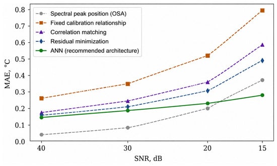
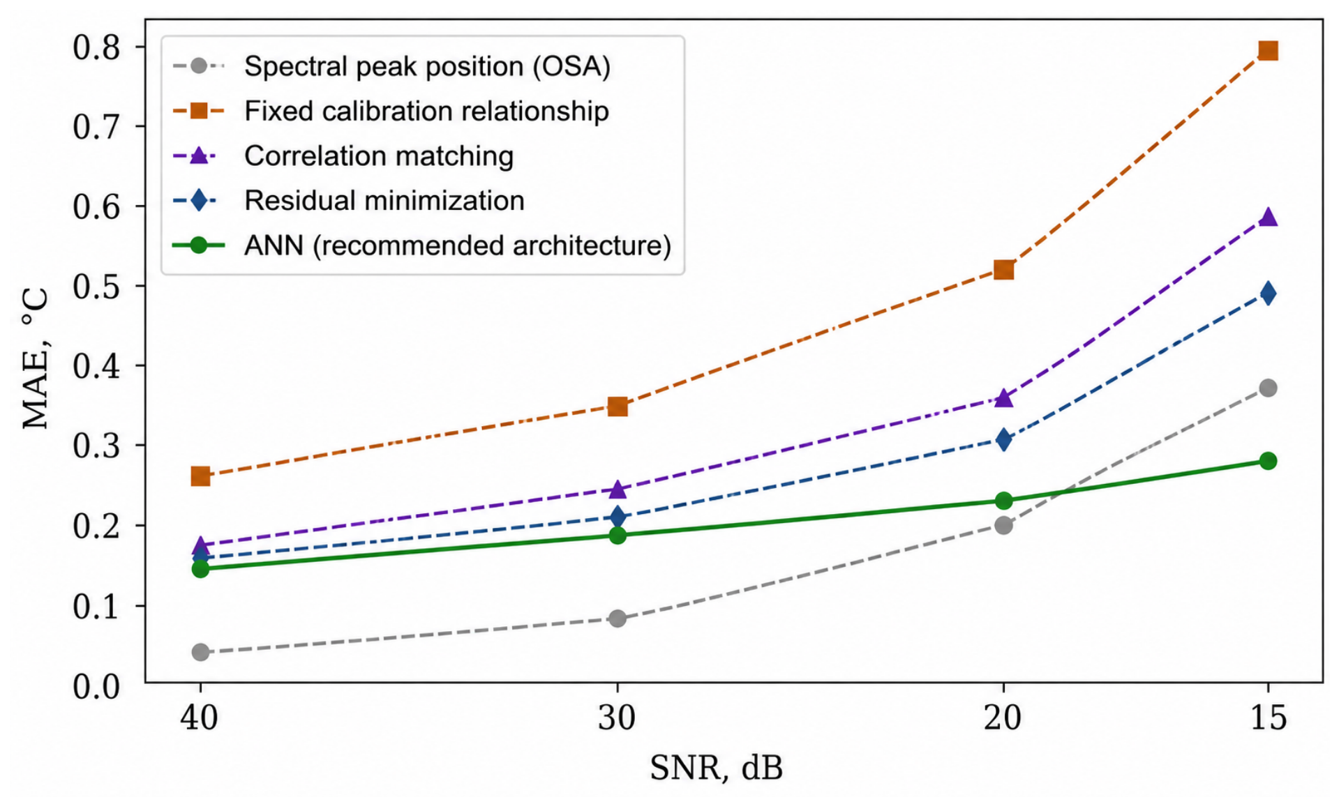
At high SNR, the spectral peak position method provides the lowest absolute reconstruction error, with an MAE of 0.052 °C at 40 dB compared with 0.148 °C for the ANN-based approach (Figure 4). However, the ANN-based reconstruction exhibits a slower degradation in accuracy as the noise level increases. When the SNR decreases from 40 to 15 dB, the MAE increases by 0.164 °C for the ANN, compared with 0.320, 0.541, 0.411, and 0.336 °C for the spectral peak position, fixed calibration, correlation matching, and residual minimization methods, respectively. At 15 dB, the ANN-based approach therefore yields the lowest MAE among the considered methods, 0.312 °C. These results indicate that the combination of a multidimensional MPRV representation and regression trained on noise-corrupted data provides increased robustness to degradation of the measurement conditions.
Figure 4.
Dependence of the MAE of temperature reconstruction on the noise level for different interrogation methods.
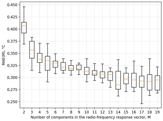
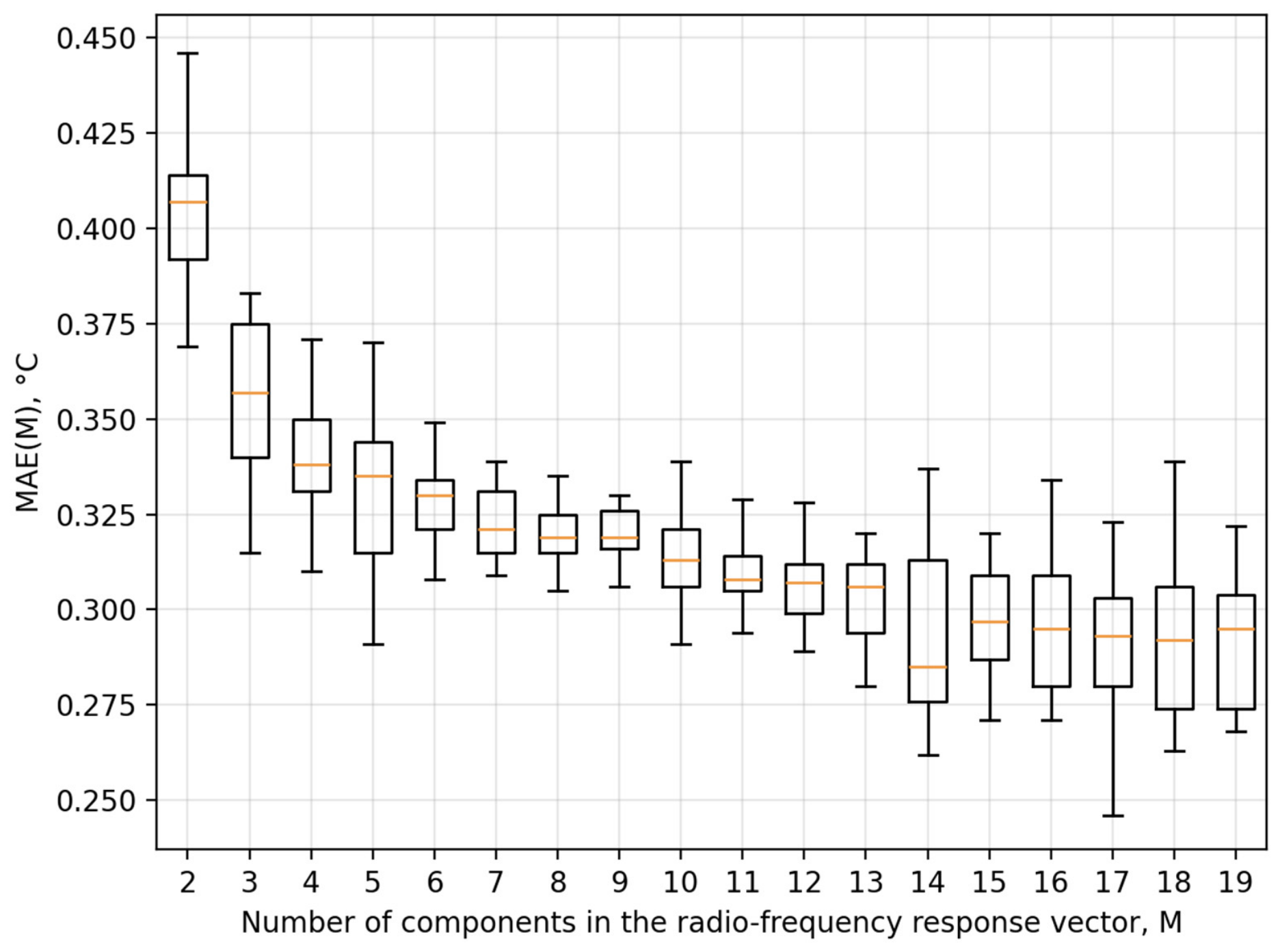
The influence of the number of components in the radio-frequency response vector on the measurement accuracy was also studied. The diagram demonstrating the value of mean absolute error (MAE) of the temperature sensing with a varying number of components of the radio-frequency response vector is presented in Figure 5.
Figure 5.
Dependence of the MAE of temperature reconstruction on the number of components in the radio-frequency response vector.
The most significant improvement in accuracy is observed when the number of components in the radio-frequency response vector is increased from 2 to 7–9. With two components, the MAE is approximately 0.41 °C; with 3–4 components, it is about 0.36 °C; with 5–6 components, it is 0.33–0.34 °C; and with 7–9 components, the MAE drops to 0.30–0.31 °C, reducing by approximately 25% relative to the initial value.
Further increasing the number of components yields no significant reduction in error. In the range of 9–19 components, the MAE values generally remain between 0.29 °C and 0.32 °C. The minimum values—around 0.29 °C—are reached at 15–16 components; however, the gain compared to using 7–9 components is marginal. This fact indicates that the information content of the RF response reaches a point of saturation. The initially added components significantly enhance the distinguishability of the sensing element’s states; however, as more components are included, the new features become highly correlated with those already present, failing to provide a proportional increase in accuracy. An additional constraint is the shape of the sensing element’s spectral response. In the wavelength ranges with a small local gradient of the spectrum—specifically near the reflection peak of the FBG—increasing the number of spectral components does not lead to a significant increase in sensitivity. Furthermore, increasing the dimensionality of the vector does not resolve potential ambiguities where distinct spectral positions result in similar RF responses.
Increasing the number of OFC components also places greater demands on the measurement chain. For a fixed frequency step, an increase in the number of components leads to a greater spectral width of the probe signal, a higher maximum difference frequency, a wider required bandwidth for the photodetector and radio-frequency signal paths, a higher sampling rate, and a larger volume of data to be processed. For the configuration studied, a range of 7–9 components is optimal, as stated above. However, the optimal number of components is not universal; it depends on the shape and width of the sensing element’s spectral response, the frequency step, the operating spectral range, the noise level, and the range of temperature variation. A practical criterion for selection is to reach a dimensionality for the RF response beyond which any further increase in the number of components does not lead to a statistically significant reduction in the reconstruction error.
The robustness of the method to parametric variations in the measurement path that were not accounted for during the initial calibration was additionally investigated. The considered perturbations included increased nonuniformity of the OFC line amplitudes and residual source-power drift after normalization using the reference channel. When the OFC line-amplitude nonuniformity was increased by 1 and 2 dB, the additional error of the neural-network method was 0.04 and 0.07 °C, respectively, whereas for the fixed calibration relationship method it was 0.18 and 0.37 °C. For residual optical-power drifts of 5% and 10%, the corresponding additional errors were 0.02 and 0.05 °C for the ANN, compared with 0.09 and 0.21 °C for the fixed calibration relationship method. Thus, under the investigated conditions, the additional error of the neural-network method was approximately 4–5 times lower. The observed robustness is determined not only by the selected ANN architecture but, more importantly, by incorporating the corresponding variations in the measurement-path parameters into the training dataset, enabling the network to account for their influence when reconstructing the measurand.
In addition to accuracy and noise robustness, an important advantage of neural-network-based reconstruction is its high computational speed after training has been completed. In the computational experiments performed, the time required to obtain a single estimate did not exceed 0.1 ms, whereas iterative residual minimization required approximately 5–30 ms. Optical-spectrum-based interrogation is additionally constrained by the acquisition time and, in scanning systems, by the scanning speed of the spectral analyzer. This makes the proposed algorithm a promising approach for real-time interrogation of fiber-optic sensors.
It is important to note that despite the symmetrical response of the FPI relative to its peak amplitude, the unambiguous definition of temperature based on the combined FPI-FBG sensor spectral response is demonstrated in the considered temperature range, as shown in Figure 2 and Figure 3, which is mostly enabled by the asymmetric Fano resonance appearing in the spectral response near the FBG reflectance peak.
To contextualize the metrological characteristics of the proposed method against state-of-the-art conventional and microwave-photonic techniques, it is necessary to compare their fundamental resolution limits, dynamic range constraints, and hardware complexity. Conventional optical interrogation systems, such as those based on optical spectrum analyzers (OSAs) [4], tunable lasers [5], or arrayed waveguide gratings (AWGs) [6,12], achieve ultra-high metrological resolution (typically in the sub-picometer to picometer range) by directly resolving the optical spectrum. In particular, AWG-based multichannel systems have demonstrated mean wavelength reconstruction errors of 0.2–2 pm with electrical bandwidths of approximately 5.5 MHz [12], while self-compensated optoelectronic readout circuits achieve pm-level resolution with enhanced long-term reliability [13].
Wavelength-to-time mapping techniques using dispersive elements and Gaussian filters have demonstrated measurement errors below 20 pm at ultra-fast acquisition rates up to hundreds of MHz [10], and mode-locked laser schemes operate at repetition rates of 5–8 MHz. High-speed wavelength interrogation based on crossed HiBi-FLMs has demonstrated rates of 200 kHz with scalability to hundreds of MHz [32]. However, this resolution and speed come at the cost of expensive precision optomechanics, bulky dispersive elements, or high sensitivity to environmental temperature drift, which often necessitates complex active compensation circuitry [13]. Microwave-photonic techniques based on VNA sweeps, nonuniform microwave photonic filters [15], chirped microwave pulse compression with scanning bandwidths from 45 MHz to 10 GHz [14], or integrated silicon microring resonators [16] offer high speed and, in some cases, sub-picometer equivalent resolution, but are constrained by the bandwidth of the RF equipment, the complexity of arbitrary waveform generation, or the need for specialized nanofabrication.
In contrast, the proposed MPRV-based approach shifts the metrological complexity from the optical domain to the digital domain. Its theoretical spectral resolution is fundamentally bounded by the OFC line spacing and the signal-to-noise ratio of the microwave beat notes, which is inherently coarser than direct optical scanning. Nevertheless, by leveraging the multidimensional nature of the MPRV and the nonlinear interpolation capabilities of the ANN, the system achieves a temperature reconstruction MAE of 0.021 °C (equivalent to approximately 0.2 pm spectral resolution for a standard silica FBG with a sensitivity of ~10 pm/°C) at an SNR of 30 dB. Furthermore, unlike fixed-calibration edge-filter methods that suffer from severe metrological drift due to source power fluctuations [12,13], the proposed dual-channel normalized MPRV approach inherently rejects common-mode optical power drift, ensuring long-term metrological stability without active hardware feedback loops. The primary metrological limitation of the proposed method is its dynamic range, which is constrained by the requirement for a practically one-to-one mapping between the spectral position and the MPRV, necessitating careful matching of the OFC spacing to the sensor’s spectral slope.
Taken together, the obtained results show that the effectiveness of neural-network-assisted microwave-photonic interrogation is governed by three interrelated factors: the informativeness of the MPRV, selection of an operating range within which the “spectral position–MPRV” mapping remains practically one-to-one, and the representativeness of the training dataset with respect to the expected noise and parametric perturbations. When these conditions are satisfied, neural-network processing enables rapid reconstruction of the spectral shift without direct scanning of the optical spectrum and exhibits lower sensitivity to degradation of the measurement conditions.
6. Design Implications and Practical Considerations
The obtained results make it possible to formulate recommendations for the parameters of the optoelectronic path and the organization of neural-network processing that determine the practical feasibility of the proposed method. A key requirement is the matching of the OFC parameters to the spectral response of the sensing element. The number of spectral components and the inter-line frequency spacing should be selected so that several OFC lines simultaneously lie within the operating spectral range and their amplitudes change appreciably as the sensing-element spectral response shifts.
If the number of OFC lines is insufficient, both the dimensionality and informativeness of the MPRV decrease, whereas an excessive increase in the number of lines broadens the required bandwidth of the photodetection and microwave paths without necessarily improving reconstruction accuracy. The number of spectral components and the inter-line frequency spacing should therefore be selected with respect to the width and shape of the sensing-element spectral response so that several OFC lines contribute appreciably to the formation of the MPRV within the selected operating range. The linewidth of the individual OFC components should remain substantially smaller than the inter-line spacing to ensure their spectral separation.
The optimal OFC parameters are sensor-specific and should be determined with respect to the width and shape of the spectral response of the particular sensing element. Reducing the inter-line spacing increases the spectral probing density and, for a fixed probed spectral range, increases the number of OFC lines contributing to the formation of the MPRV, while simultaneously imposing stricter requirements on the frequency separation of the corresponding beat components. Conversely, an excessively large inter-line spacing may result in only one or two OFC lines interacting with the informative region of the spectral response, thereby reducing the distinguishability of MPRVs corresponding to different states of the sensing element.
The criterion for selecting the OFC parameters should therefore not be the minimization of the inter-line spacing itself, but rather the formation of several distinguishable beat components whose joint amplitude variation uniquely characterizes the spectral position of the sensing element within the selected operating range. Accordingly, the photodetector bandwidth should exceed the maximum generated difference frequency (M − 1)·Δf, while the microwave path should provide extraction of beat components over the frequency range from Δf to (M − 1)·Δf.
The selection of the operating spectral range is equally important. The simulation results show that it should be restricted to a region in which the “spectral position–MPRV” mapping remains practically one-to-one. For sensing elements with symmetric or nearly symmetric spectral responses, it is undesirable to align the central region of the OFC directly with the symmetry axis of the spectral response. In this region, different spectral positions may correspond to similar MPRVs, which fundamentally limits the accuracy of the inverse-problem solution regardless of the complexity of the neural-network model. When operation near a spectral extremum is required, the central position of the OFC should be shifted relative to the symmetry axis of the sensing-element spectral response so that the operating range is formed predominantly on one of its slopes.
To reduce the sensitivity of the reconstruction result to fluctuations in optical-source power and variations in the transmission coefficients of the measurement path, it is advisable to use a reference channel in which the response of the initial OFC is recorded before its interaction with the sensing element. In this case, the ANN input features are formed from normalized rather than absolute beat-component amplitudes. Such normalization reduces the influence of variations in the overall optical power and slow the drift in the transmission coefficients of the optoelectronic-path components while preserving information on the relative changes in the MPRV structure. Thus, the use of a reference channel and element-wise normalization forms an integral part of constructing an informative input MPRV.
For future practical implementation, the technological spread of sensing-element parameters should also be taken into account. The central wavelength and refractive-index modulation amplitude of the FBG, as well as the cavity length and refractive index of the FPI, may vary from one sensor specimen to another. A possible strategy is to pretrain a baseline neural-network model on simulated datasets covering the expected variations in sensing-element parameters, noise level, source power, and OFC line-amplitude nonuniformity, followed by fine-tuning using a limited amount of experimental data obtained for a particular sensor specimen. Such a physics-informed transfer-learning approach could reduce the amount of experimental calibration data required to adapt the interrogation system to technological variations among individual sensing elements.
The core economic advantage of the proposed architecture lies in the replacement of expensive optical scanning components (e.g., tunable lasers, OSAs, or AWGs) with a fixed OFC generator alongside standard microwave filter banks and high-speed ADCs. While a single MPRV microwave readout channel natively interrogates one sensing element, the system can be scaled to multiplex arrays of FBGs. Simultaneous interrogation of multiple FBGs can be achieved via Wavelength Division Multiplexing (WDM) using a broadband OFC; however, the maximum number of simultaneously resolvable sensors is limited by the total optical bandwidth and the microwave bandwidth of the photodetector, and separating their MPRVs in the RF domain requires complex frequency- or time-division multiplexing. A more cost-effective and practical deployment for large-scale sensor networks with tens of FBGs is to utilize low-cost optical switching combined with the proposed MPRV readout. Because the ANN inference time is strictly bounded (<0.1 ms), an optical switch can sequentially interrogate numerous sensors at aggregate kHz rates, achieving high-speed quasi-distributed sensing with significantly lower hardware cost and complexity compared to parallel AWG or OSA-based systems.
7. Conclusions
The results demonstrate that the accuracy of microwave-photonic sensor interrogation is governed primarily by the distinguishability of sensor states in the multidimensional MPRV space. When different spectral positions produce sufficiently distinct response vectors, the inverse mapping can be reconstructed with high accuracy using a neural-network model of moderate complexity. Spectral extrema and regions of symmetric alignment between the OFC and the sensing-element response give rise to similar MPRVs and therefore impose an intrinsic limitation on the inverse reconstruction. Restricting the operating range to a region with a practically one-to-one spectral position–MPRV mapping reduced the temperature reconstruction MAE from 0.198 to 0.021 °C at an SNR of 30 dB.
The proposed interrogation framework represents the sensor state by a multidimensional microwave-photonic response vector formed from the amplitudes of beat components generated at the OFC difference frequencies. This representation enables the distributed information contained in the microwave-photonic response to be used for reconstruction of the sensing-element state. Numerical analysis showed that the combination of an informative MPRV, an appropriately selected operating range, and training data incorporating noise and parametric perturbations provides increased robustness to degradation of the measurement conditions. At an SNR of 15 dB, the ANN-based reconstruction achieved the lowest MAE among the considered methods, 0.312 °C.
The proposed approach also demonstrated reduced sensitivity to OFC line-amplitude nonuniformity and residual optical-power drift. After training, the reconstruction time did not exceed 0.1 ms, indicating the potential of the method for high-speed interrogation without direct optical-spectrum scanning. These results show that the performance of neural-network-assisted microwave-photonic interrogation is determined primarily by the physical informativeness and identifiability of the MPRV representation, while the neural network serves as an efficient nonlinear estimator of the sensor state.
Author Contributions
Conceptualization, R.A.M. and A.Z.S.; methodology, A.Z.S. and O.G.M.; software, B.I.V.; validation, M.Y.F. and A.A.K.; formal analysis, A.Z.S.; investigation, T.A.A. and A.A.K.; resources, A.Z.S.; data curation, R.A.M.; writing—original draft preparation, R.A.M.; writing—review and editing, A.Z.S. and O.G.M.; visualization, B.I.V.; supervision, A.Z.S.; project administration, A.Z.S.; funding acquisition, T.A.A. and A.A.K. All authors have read and agreed to the published version of the manuscript.
Funding
This work was supported by a grant from the Russian Science Foundation, project no. 23-79-10059-П.
Data Availability Statement
The data presented in this study are available from the corresponding author upon reasonable request.
Conflicts of Interest
The authors declare no conflicts of interest.
Abbreviations
The following abbreviations are used in this manuscript:
| ADC | Analog-to-Digital Converter |
| ANN | Artificial Neural Network |
| FBG | Fiber Bragg Grating |
| FPI | Fabry–Pérot Interferometer |
| MAE | Mean Absolute Error |
| MPRV | Microwave-Photonic Response Vector |
| MTOS | Multi-Tone Optical Signal |
| OFC | Optical Frequency Comb |
| OSA | Optical Spectrum Analyzer |
| ReLU | Rectified Linear Unit |
| SNR | Signal-to-Noise Ratio |
References
- Dey, K.; Vangety, N.; Roy, S. Machine Learning Approach for Simultaneous Measurement of Strain and Temperature Using FBG Sensor. Sens. Actuators A Phys. 2022, 333, 113254. [Google Scholar] [CrossRef] [Scilit]
- Costa, G.K.B.; Gouvêa, P.M.P.; Soares, L.M.B.; Pereira, J.M.B.; Favero, F.; Braga, A.M.B.; Palffy-Muhoray, P.; Bruno, A.C.; Carvalho, I.C.S. In-Fiber Fabry-Perot Interferometer for Strain and Magnetic Field Sensing. Opt. Express 2016, 24, 14690–14696. [Google Scholar] [CrossRef] [Scilit] [PubMed]
- Yang, J.; Zhao, Z.; Li, X.; Li, X.; Yang, W. A Cryogenic Liquid Level Sensor Based on EFPI-FBG. Measurement 2026, 257, 118842. [Google Scholar] [CrossRef] [Scilit]
- Baney, D.M.; Szafraniec, B.; Motamedi, A. Coherent Optical Spectrum Analyzer. IEEE Photonics Technol. Lett. 2002, 14, 355–357. [Google Scholar] [CrossRef] [Scilit]
- Clement, J.; Torregrosa, G.; Maestre, H.; Fernández-Pousa, C.R. Remote Picometer Fiber Bragg Grating Demodulation Using a Dual-Wavelength Source. Appl. Opt. 2016, 55, 6523–6529. [Google Scholar] [CrossRef] [Scilit] [PubMed]
- Culshaw, B. Optical Fiber Sensor Technologies: Opportunities and—Perhaps—Pitfalls. J. Light. Technol. 2004, 22, 39–50. [Google Scholar] [CrossRef] [Scilit]
- Li, B.; Tan, Z.-W.; Shum, P.P.; Wang, C.; Zheng, Y.; Wong, L. Dilated Convolutional Neural Networks for Fiber Bragg Grating Signal Demodulation. Opt. Express 2021, 29, 7110–7123. [Google Scholar] [CrossRef] [Scilit] [PubMed]
- Cao, Z.; Zhang, S.; Xia, T.; Liu, Z.; Li, Z. Spectral Demodulation of Fiber Bragg Grating Sensor Based on Deep Convolutional Neural Networks. J. Light. Technol. 2022, 40, 4429–4435. [Google Scholar] [CrossRef] [Scilit]
- Wu, Y.; Xia, L.; Wu, N.; Wang, Z.; Zuo, G. Optimized Feedforward Neural Network for Multiplexed Extrinsic Fabry-Perot Sensors Demodulation. J. Light. Technol. 2021, 39, 4564–4569. [Google Scholar] [CrossRef] [Scilit]
- Fernández, M.P.; Bulus Rossini, L.A.; Cruz, J.L.; Andrés, M.V.; Costanzo Caso, P.A. High-Speed and High-Resolution Interrogation of FBG Sensors Using Wavelength-to-Time Mapping and Gaussian Filters. Opt. Express 2019, 27, 36815–36823. [Google Scholar] [CrossRef] [Scilit] [PubMed]
- Madrigal, J.; Fraile-Peláez, F.J.; Zheng, D.; Barrera, D.; Sales, S. Characterization of a FBG Sensor Interrogation System Based on a Mode-Locked Laser Scheme. Opt. Express 2017, 25, 24650–24657. [Google Scholar] [CrossRef] [Scilit] [PubMed]
- Marrazzo, V.R.; Fienga, F.; Riccio, M.; Irace, A.; Breglio, G. Multichannel Approach for Arrayed Waveguide Grating-Based FBG Interrogation Systems. Sensors 2021, 21, 6214. [Google Scholar] [CrossRef] [Scilit] [PubMed]
- Marrazzo, V.R.; Fienga, F.; Riccio, M.; Irace, A.; Breglio, G. New Self-Compensated Optoelectronic Circuit for Highly Reliable Read-Out of FBG Sensor Arrays. IEEE Sens. J. 2025, 25, 24106–24114. [Google Scholar] [CrossRef] [Scilit]
- Xu, O.; Zhang, J.; Yao, J. High Speed and High Resolution Interrogation of a Fiber Bragg Grating Sensor Based on Microwave Photonic Filtering and Chirped Microwave Pulse Compression. Opt. Lett. 2016, 41, 4859–4862. [Google Scholar] [CrossRef] [Scilit] [PubMed]
- Xiao, D.; Shao, L.; Wang, C.; Lin, W.; Yu, F.; Wang, G.; Ye, T.; Wang, W.; Vai, M.I. Optical Sensor Network Interrogation System Based on Nonuniform Microwave Photonic Filters. Opt. Express 2021, 29, 2564–2576. [Google Scholar] [CrossRef] [Scilit] [PubMed]
- Zhu, Z.; Wang, Q.; Sun, J.; Hu, G.; Yun, B.; Cui, Y. On-Chip High-Precision Microwave Photonic FBG Interrogation System Based on a Silicon Microring Resonator. Opt. Laser Technol. 2026, 204, 116253. [Google Scholar] [CrossRef] [Scilit]
- Hervas, J.; Ricchiuti, A.L.; Li, W.; Zhu, N.H.; Fernandez-Pousa, C.R.; Sales, S.; Li, M.; Capmany, J. Microwave Photonics for Optical Sensors. IEEE J. Sel. Top. Quantum Electron. 2017, 23, 327–339. [Google Scholar] [CrossRef] [Scilit]
- Ricchiuti, A.L.; Barrera, D.; Sales, S.; Thevenaz, L.; Capmany, J. Long Fiber Bragg Grating Sensor Interrogation Using Discrete-Time Microwave Photonic Filtering Techniques. Opt. Express 2013, 21, 28175. [Google Scholar] [CrossRef] [Scilit] [PubMed]
- Morozov, O.; Sakhabutdinov, A.; Anfinogentov, V.; Misbakhov, R.; Kuznetsov, A.; Agliullin, T. Multi-Addressed Fiber Bragg Structures for Microwave-Photonic Sensor Systems. Sensors 2020, 20, 2693. [Google Scholar] [CrossRef] [Scilit] [PubMed]
- Cybenko, G. Approximation by Superpositions of a Sigmoidal Function. Math. Control Signals Syst. 1989, 2, 303–314. [Google Scholar] [CrossRef] [Scilit]
- Hornik, K.; Stinchcombe, M.; White, H. Multilayer Feedforward Networks Are Universal Approximators. Neural Netw. 1989, 2, 359–366. [Google Scholar] [CrossRef] [Scilit]
- Agliullin, T.A.; Sakhabutdinov, A.Z.; Kuznetsov, A.A.; Valeev, B.I. Conditions for Fano Resonance Occurrence in Combined Fiber Quasiperiodic Structures. J. Opt. Technol. 2025, 92, 296–302. [Google Scholar] [CrossRef] [Scilit]
- Sakhabutdinov, A.; Agliullin, T.A.; Hussein, S.M.R.H.; Kuznetsov, A.A.; Anfinogentov, V.I.; Valeev, B.I. Fano-Type Resonance Structures Based on Combination of Fiber Bragg Grating with Fabry-Perot Interferometer. Karbala Int. J. Mod. Sci. 2023, 9, 3. [Google Scholar] [CrossRef] [Scilit]
- Liu, Y.; Liu, X.; Zhang, T.; Zhang, W. Integrated FPI-FBG Composite All-Fiber Sensor for Simultaneous Measurement of Liquid Refractive Index and Temperature. Opt. Lasers Eng. 2018, 111, 167–171. [Google Scholar] [CrossRef] [Scilit]
- Diddams, S.A.; Vahala, K.; Udem, T. Optical Frequency Combs: Coherently Uniting the Electromagnetic Spectrum. Science 2020, 369, eaay3676. [Google Scholar] [CrossRef] [Scilit] [PubMed]
- Torres-Company, V.; Weiner, A.M. Optical Frequency Comb Technology for Ultra-Broadband Radio-Frequency Photonics. Laser Photonics Rev. 2014, 8, 368–393. [Google Scholar] [CrossRef] [Scilit]
- Agliullin, T.; Il’In, G.; Kuznetsov, A.; Misbakhov, R.; Misbakhov, R.; Morozov, G.; Morozov, O.; Nureev, I.; Sakhabutdinov, A. Overview of Addressed Fiber Bragg Structures’ Development. Photonics 2023, 10, 175. [Google Scholar] [CrossRef] [Scilit]
- Miliou, A. In-Fiber Interferometric-Based Sensors: Overview and Recent Advances. Photonics 2021, 8, 265. [Google Scholar] [CrossRef] [Scilit]
- Zhou, X.; Ma, F.; Ling, H.; Yu, B.; Peng, W.; Yu, Q. A Compact Hydrogen Sensor Based on the Fiber-Optic Fabry-Perot Interferometer. Opt. Laser Technol. 2020, 124, 105995. [Google Scholar] [CrossRef] [Scilit]
- Erdogan, T. Fiber Grating Spectra. J. Light. Technol. 1997, 15, 1277–1294. [Google Scholar] [CrossRef] [Scilit]
- Chai, S.; Guo, C.; Guan, C.; Fang, L. Deep Learning-Based Speech Enhancement of an Extrinsic Fabry–Perot Interferometric Fiber Acoustic Sensor System. Sensors 2023, 23, 3574. [Google Scholar] [CrossRef] [Scilit] [PubMed]
- Ding, Z.; Tan, Z.; Wang, Y. High-Speed Wavelength Interrogation System Based on Crossed HiBi-FLMs for Array FBGs. Opt. Fiber Technol. 2022, 74, 103138. [Google Scholar] [CrossRef] [Scilit]

Disclaimer/Publisher’s Note: The statements, opinions and data contained in all publications are solely those of the individual author(s) and contributor(s) and not of MDPI and/or the editor(s). MDPI and/or the editor(s) disclaim responsibility for any injury to people or property resulting from any ideas, methods, instructions or products referred to in the content. |
© 2026 by the authors. Licensee MDPI, Basel, Switzerland. This article is an open access article distributed under the terms and conditions of the Creative Commons Attribution (CC BY) license.