


Abstract
Public brain metastasis MRI cohorts are widely used for prognostic modeling, but whether an endpoint is identifiable at the available sample size is rarely tested. We evaluated eight clinical endpoints in two public cohorts, Yale/BraTS-MET (199 patients, 74 deaths) and OpenBTAI/MOLAB (75 patients, all deceased), using lesion-centered nnU-Net encoder embeddings and PyRadiomics features with patient-grouped cross-validation and label permutation. Patient-level infratentorial involvement served as a positive control (balanced accuracy 0.60); the Graded Prognostic Assessment (GPA) score was recoverable from OpenBTAI radiomics ( = 0.42), whereas brain age was not recovered in either cohort. Primary tumor type was the only endpoint significant after multiplicity correction (1.3× chance). Survival endpoints were null for clinical models and the planned graph model (C = 0.50, p = 0.49); an exploratory linear model on embeddings reached C ≈ 0.58 (p = 0.07, uncorrected), which PyRadiomics features did not reproduce. No progression definition remained significant after family-wise correction. In simulation, 80% power required a true C-index of about 0.68–0.76, so null survival results cannot exclude moderate effects. GPA did not stratify survival (p = 0.18) in a cohort containing only deceased patients. An extraction error found during revision was corrected.
1. Introduction
Accurate prognostication in patients with brain metastases informs treatment selection and patient counseling, and prognostic indices such as the Graded Prognostic Assessment (GPA) [1] are in routine clinical use. Data-driven prognostic modeling from MRI has attracted growing interest, as part of a broader move toward multimodal artificial intelligence in oncology [2,3]. In brain metastases specifically, machine-learning models have been proposed for treatment response and local control [4,5,6], post-radiosurgery adverse effects such as radiation necrosis [7,8], and mutation status [9], and several systematic reviews now summarize this literature [10,11,12,13]. Public resources have lowered the barrier to entry: curated private cohorts with survival data are scarce and expensive to assemble, whereas BraTS-MET on TCIA (200 cases with expert segmentations, 199 with usable survival data) [14] and MOLAB/OpenBTAI (75 cases with longitudinal imaging) [15] are freely available.
Yet results reported on the same public cohort can differ substantially. On Yale/BraTS-MET, for example, a recent study reported a survival-time regression with = 0.97 [16], whereas the patient-grouped, censoring-aware evaluation used here finds no survival signal distinguishable from chance. Protocol choices such as the handling of censored patients and the unit of scoring can produce differences of this kind (Appendix A); we did not attempt to reproduce that study.
Multimodal and graph-based survival models have been proposed for other tumor types [17,18,19,20,21], as have general frameworks for survival analysis with medical data [22], and the present evaluation includes a lesion-level graph model (E1c). For a group deciding what to do next, the practical question is as follows: at this scale of data, which endpoints are identifiable, and can this be established before months of model development is committed?
Accordingly, the aim of this study was to determine, using positive controls, patient-grouped permutation testing, and effect-size bounds, which prognostic and treatment-response endpoints are identifiable from two public brain metastasis MRI cohorts at their available sample sizes.
A positive control, an endpoint that a pipeline with genuine sensitivity should recover, together with a label-permutation null for every real endpoint, turns the statement that a model did not beat chance into a calibrated one. A control cannot, however, certify sensitivity to a different kind of signal, and a null result is informative only to the extent that the power for plausible effects is known. We, therefore, combined positive controls of several kinds, patient-grouped permutation tests, family-wise correction for the freedom in endpoint definitions, and a semi-synthetic power simulation, and we report how each step changed the strength of what could be concluded. Methodological guidance on small-sample prognostic modeling already exists [23,24,25,26,27,28]; our aim is to quantify its consequences in one concrete setting.
The contributions of this study are as follows:
- Positive controls and null results for eight planned endpoints in two public cohorts, with the limits of each control stated.
- A semi-synthetic power simulation showing that the imaging survival pipeline reaches 80% power only for strong effects (true C-index of about 0.68–0.76).
- A quantification of researcher freedom in endpoint definition: 18 definitions of lesion progression, with family-wise correction.
- A documented feature-extraction error, its correction, and a proposed pre-flight checklist that incorporates it.
- Open code and intermediate results.
2. Materials and Methods
2.1. Study Design
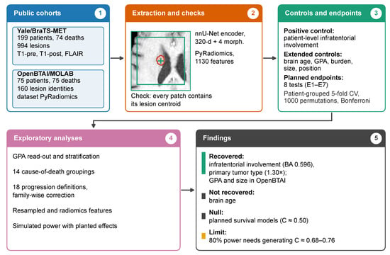
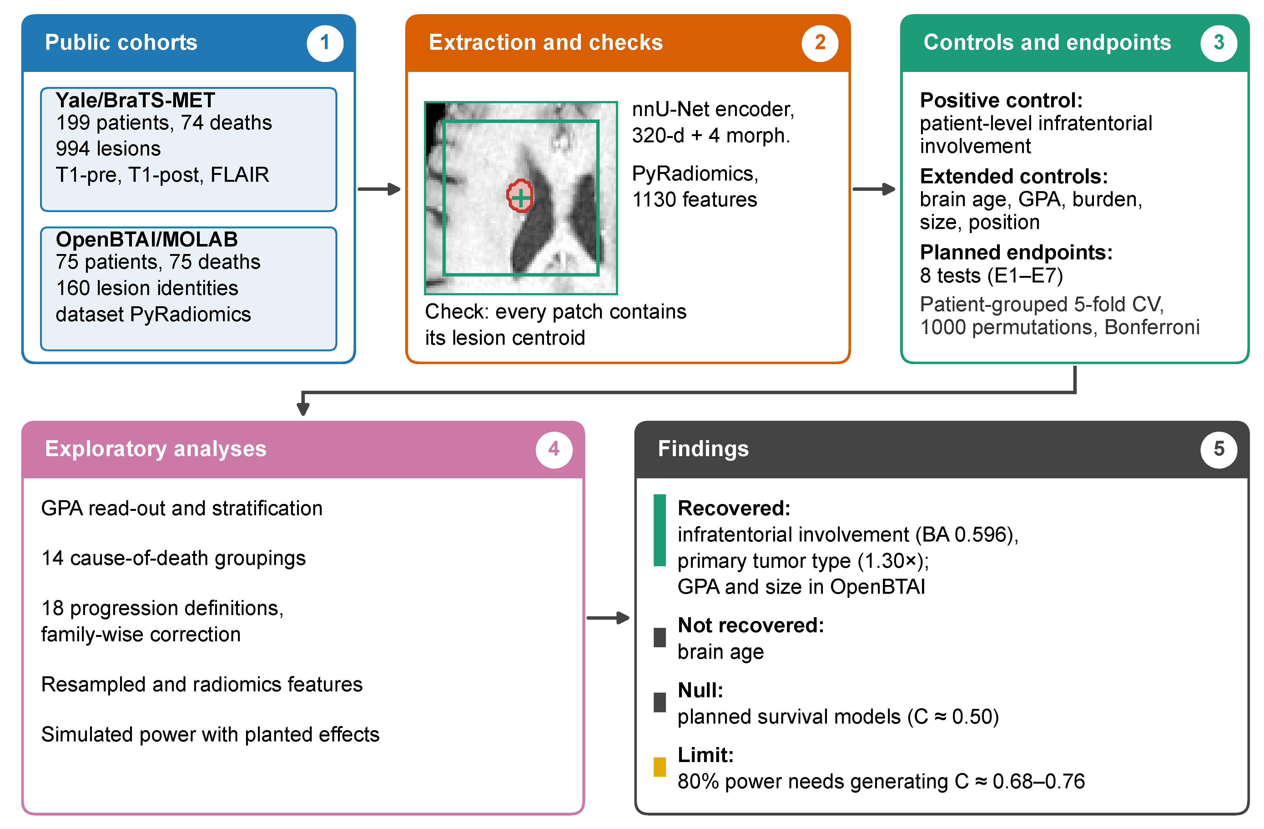
We evaluated eight planned clinical endpoints and one anatomical positive control in two cohorts. Because the cohorts differ in features, endpoints and follow-up, the study consists of two parallel single-cohort analyses that share one validation protocol (Section 2.5); it is not a pooled evaluation. Analyses designed after the first results are labeled exploratory (Figure 1).
Figure 1.
Evaluation workflow. (1) Two public cohorts. (2) Feature extraction, with a check that every patch contains its lesion centroid; the example shows a lesion mask (red) and its patch (green). (3) Positive controls and planned endpoints under one validation protocol. (4) Exploratory analyses. (5) Main findings.
2.2. Cohorts and Data Audit
Yale/BraTS-MET. The cohort [14] provides T1-precontrast, T1-postcontrast and T2-FLAIR MRI with expert segmentations. Of 200 cases, one was excluded for missing outcome data, leaving 199 (74 deaths, 125 censored; median follow-up 15.8 months). Lesions were defined as 26-connected components of the enhancing label (minimum 3 voxels), giving 994 lesions (993 analyzed). A minimum of 5 voxels reproduces the dataset’s official count of 975 exactly; our rule adds 19 fragments of 3–4 voxels (1.9%). The release contains no treatment variables.
OpenBTAI/MOLAB. The cohort [15] provides 75 patients, all deceased (median survival 723 days), with 373 segmented time points and lesion-level PyRadiomics features. Lesion labels are renumbered between time points in 31 of 75 patients, which explains why the 160 label identities exceed the 154 distinct lesions in the data descriptor. Cause of death was recorded for 69 patients and GPA for 68; 72 patients received stereotactic radiosurgery and 48 whole-brain radiotherapy (Table 1).
Table 1.
Characteristics of the two public cohorts.
Data audit and ethics. Mask volumes agreed with the dataset’s morphology tables (median ratio 1.000; n = 495), and the clinical table was cross-checked against the source spreadsheet cell by cell. Of 373 OpenBTAI masks, 339 were in RAS and 34 in LAS orientation (two patients inconsistent within their series); no OpenBTAI survival model uses coordinate-dependent features. The separate location-axis control uses first-record centroids from all 74 patients; these centroids are physical (RAS world) coordinates in millimeters obtained from each image affine, so the 34 LAS masks require no reorientation; the axis-wise results are given in Supplement S8. All 200 Yale images and masks are in RAS orientation. All data are public and de-identified; approvals and licenses are given in the Institutional Review Board and Data Availability statements.
2.3. Imaging Features
Yale. Lesion embeddings were extracted with a 3D nnU-Net encoder [29] pretrained for brain metastasis segmentation on UCSF-BMSR [30] (details in Supplement S1). For each lesion, the three sequences were used on their native grid, z-scored per channel and cropped to a patch centered on the lesion-mask centroid; the 320-channel bottleneck feature map was averaged over space. Four morphology features (log-volumes of enhancing tumor, necrosis and edema, and the edema-to-tumor ratio) were appended. Patient-level analyses used the within-patient mean; lesion-level analyses (positive control, graph model) kept lesions as units with patient-grouped folds. Two secondary representations were computed: embeddings from images resampled to 1.0 mm, and PyRadiomics features (1130 per lesion, settings aligned with OpenBTAI; five lesions failed).
Extraction error. During revision, we found that our first extraction had read the centroid table, whose columns are stored in (z, y, x) order under the names x, y, z, in the wrong axis order. Patches were, therefore, centered on positions with the left–right and superior–inferior coordinates exchanged: only 38% overlapped the lesion mask at all, and the median distance between patch center and lesion centroid was 68 mm. The archived embeddings were reproduced bit for bit from the original table, which identifies the cause. All analyses that depend on the embeddings, including the graph model and its edge features, were repeated with centroids recomputed from the expert masks (every corrected patch contains its lesion centroid); results of the first extraction are in Supplement S7. No extraction log of the first run had been kept. Analyses based on clinical variables or on the OpenBTAI radiomics were not affected.
OpenBTAI. The 1130 PyRadiomics features distributed with the dataset (Total region) were used as released [15]; for patient-level analyses, lesion features were summarized by the within-patient median (settings in Supplement S1).
2.4. Endpoints and Controls
Planned endpoints. The endpoints (Table 2) and the positive control were defined in internal project files before results were examined; because there was no external registration, we call them planned rather than pre-registered. After the first results, the number of permutations was raised from 100 to 1000, and the two Yale clinical survival models (E1, E1b) were counted as one endpoint with E1b as primary. Multiplicity was handled by Bonferroni correction across eight endpoints ( = 0.0063; = 0.0042 if each of 12 reported tests is counted).
Table 2.
Planned endpoints and positive control, with the observed value and the permutation p-value.
Positive-control label. The control label is the clinical-table field “presence of metastasis in infratentorial region”, which is recorded per patient (91 of 199 patients positive). Every lesion inherits its patient’s label, balanced accuracy is computed over lesions, and permutation is performed at the patient level. Patients with lesions in both compartments, therefore, contribute some mislabeled supratentorial lesions, which can only lower the observed accuracy; no lesion-level reference exists (Supplement S1).
Cause of death (E5). The source workbook codes cause of death as 1–4. An unlabeled legend block placed next to the death columns (cells BU9–BU12) lists 1, brain progression; 2, systemic illness; 3, systemic plus brain progression (text truncated in the workbook andd 4, other. We take it as the legend of the Cause column; the data descriptor does not define the codes. Each patient was assigned the code of the first lesion row (two patients carry different codes in different rows). The codes were 1 (n = 8), 2 (n = 23), 3 (n = 29) and 4 (n = 8); one composite 1 + 4 entry and six blanks were treated as missing, leaving 68 usable codes. E5 contrasts codes 1 or 3 (brain involved) with 2 or 4. Counting a patient as brain-involved if any row carries code 1 or 3 raises the number of brain-involved deaths from 37 to 38 and changes none of the conclusions (Supplement S4).
GPA and necrosis. GPA and radiation necrosis are recorded per lesion row; we used the first row. Three patients have conflicting GPA values, and an any-row necrosis definition raises the number of events from 26 to 28; alternative rules change no conclusion (Supplement S4).
The two Yale clinical survival models use the clinical table regenerated on 18 September 2026, which differs from the earlier version in two race indicator columns (Supplement S1).
2.5. Validation and Statistical Analysis
All analyses used stratified 5-fold cross-validation grouped by patient, within-fold standardization, and simple regularized linear, logistic or Cox models with fixed hyperparameters (Ridge = 10; logistic C = 0.1 with balanced weights; Cox penalizer from a fixed ladder, using the first value that converged). Significance was assessed by permuting the patient-to-label mapping, with empirical p = P(null ≥ observed). The smallest attainable value is 1/(P + 1), so we write p ≤ 0.001 when none of 1000 null values reached the observed one (p ≤ 0.005 for 200 permutations). Sensitivity to the regularization settings and a nested-tuning variant are in Supplement S2 and change no conclusion. The graph model (E1c; GATv2 with a global node and five edge features) used nested validation with ten training seeds on fixed folds, together with 50 label permutations (Supplement S1). C-index conventions differ by endpoint and are given in the footnote of Table 2. Confidence intervals for out-of-fold metrics are patient-level bootstrap percentile intervals (2000 resamples) and reflect evaluation variance only; for E1, E1b, E2 and E3 the interval is translated to the reported estimate (Supplement S1).
Extended positive controls. Brain age, log intracranial burden, largest-lesion diameter, age, lesion count, sex, receipt of radiosurgery and necrosis were predicted from the same representations under the same protocol, so that the calibration of each cohort rests on several targets rather than one; the three spatial axes of the first-record lesion were used as an additional, continuous location target.
GPA analyses. We predicted the recorded GPA from OpenBTAI radiomics (patient-level Ridge; n = 67) and examined GPA against survival (log-rank, n = 68) and against age, lesion count and log intracranial burden. Partial correlations controlled for these variables, and GPA was additionally permuted within primary tumor type. KPS and extracranial disease status are not recorded, so the decomposition covers recorded components only.
Endpoint-definition grid. Lesion progression was defined in 18 ways (reference frame: landmark or nadir; window: any time, 180 or 365 days; threshold: ×1.2, ×1.35 or ×1.5) on the same 90 landmark-eligible OpenBTAI lesions from 61 patients, with a patient-grouped Cox model on seven features. Permutation was performed at the patient level: the outcome records of whole patients were exchanged among patients with the same number of lesions (strata of 1, 2 and 4 lesions), so that each patient’s lesions moved together. A lesion-level permutation, which shuffles lesions independently, is reported as a sensitivity analysis. Family-wise error was assessed with a Westfall–Young [31] max-statistic procedure over 1000 shared permutations, in which one patient-to-outcome mapping is applied to all 18 cells; single-cell p-values use independent permutations. The nadir reference uses follow-up after the landmark.
All growth thresholds in this study are volumetric. Because volume scales with the cube of diameter, a 20% increase in diameter corresponds to an increase of approximately 73% in volume (); the 20% volumetric threshold used for E3 is, therefore, considerably more sensitive than the diameter-based RANO-BM progression criterion [32,33].
Upper limits and power. Upper limits are the observed C-index plus 1.96 times a standard deviation (the permutation-null SD; for the graph model also the SD over training seeds). They are rough guides and not formal exclusions. To calibrate power, we planted known effects in the real Yale feature space (324 features, 199 patients, 63% censoring): exponential proportional-hazards survival times were generated from a linear predictor whose direction was either concentrated in the first five principal components or dense across all 324 dimensions, with effects set so that the generating C-index was 0.55, 0.60, 0.65 or 0.70. The complete pipeline (patient-grouped 5-fold Cox, 100 label permutations) was run on 50 replicates per setting and on 200 replicates under no effect.
3. Results
3.1. Positive Controls
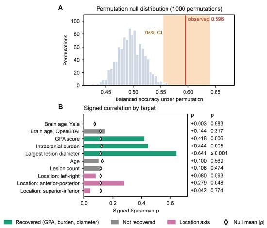
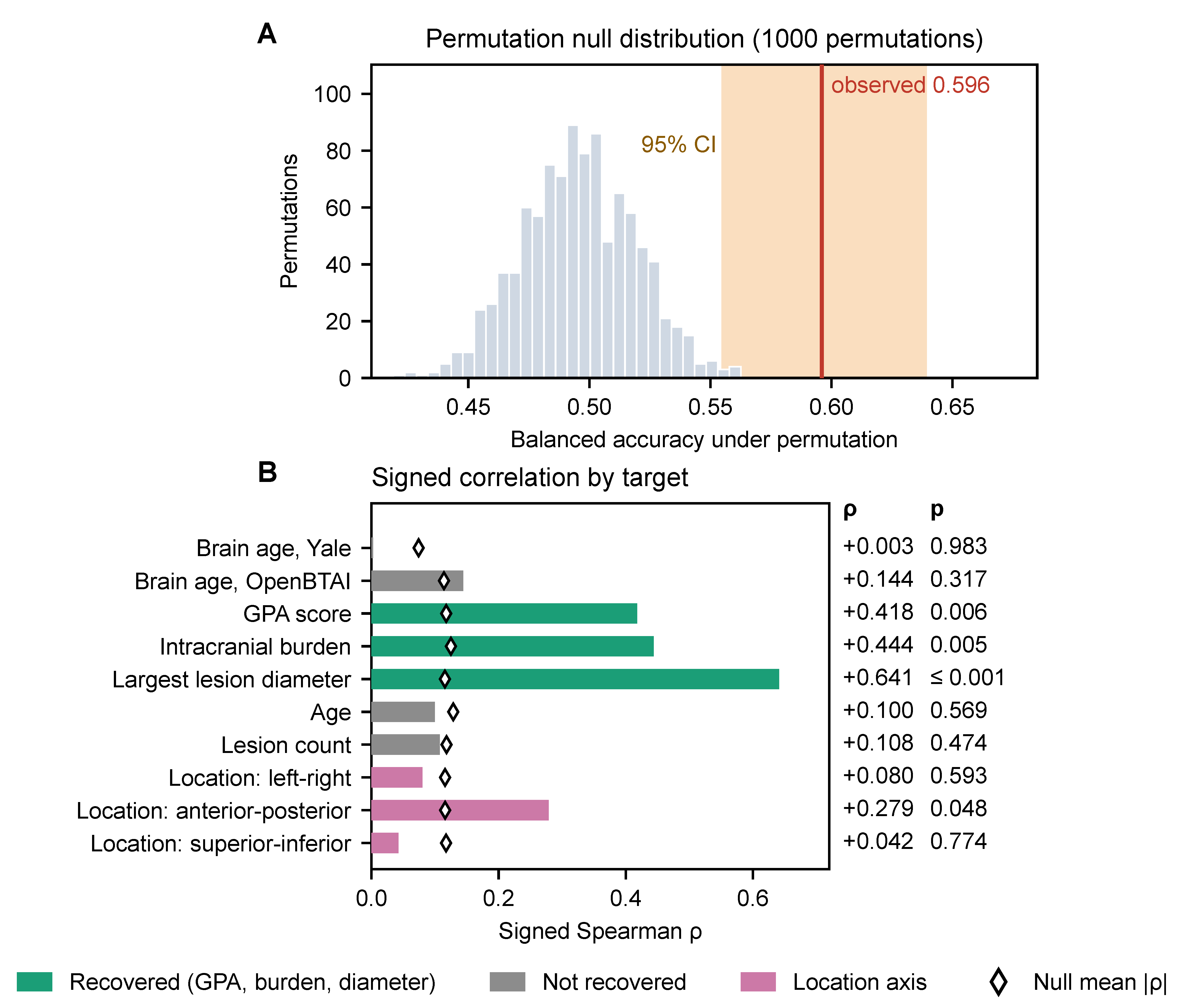
Patient-level infratentorial involvement was recovered from the lesion-centered embeddings (balanced accuracy 0.596, 95% CI 0.555–0.639; permutation null 0.496 ± 0.023; p ≤ 0.001; Figure 2A) and with 1.0 mm resampling (0.585). The effect is modest (1.2× chance) for a property that is evident on the images, and label noise from patient-level labeling may contribute; the control, therefore, certifies sensitivity only to weak, diffuse signals in Yale, and “detectable” should not be read as “usable”. PyRadiomics features of the lesion mask, which carry no spatial context, did not recover location (balanced accuracy 0.50, p = 0.48). Brain age [34] was not recovered in Yale ( = 0.003, p = 0.98) or in OpenBTAI ( = 0.14, p = 0.32); the association seen in our first extraction ( ≈ 0.17–0.23) did not persist with lesion-centered patches (Supplement S7).
Figure 2.
Positive controls. (A) Permutation null distribution (1000 patient-grouped permutations) of the balanced accuracy for patient-level infratentorial involvement (present versus absent); the line marks the observed value (0.596) and the shaded band its patient-level bootstrap 95% CI (0.555–0.639). (B) Signed Spearman between out-of-fold predictions and targets for the extended controls (green: recovered from radiomics; grey: not recovered; pink: location axes; diamonds: mean absolute under the permutation null). GPA and lesion count: n = 67; location axes: n = 74 (Supplement S8). p-values are not corrected for multiplicity.
In OpenBTAI, radiomics recovered the GPA score ( = 0.42, p = 0.006, n = 67), log intracranial burden ( = 0.44, p = 0.005) and largest-lesion diameter ( = 0.64, p ≤ 0.001), but not age, lesion count, SRS receipt or necrosis. Position along the left–right, anterior–posterior and superior–inferior axes gave = 0.08, 0.28 and 0.04 (p = 0.59, 0.048 and 0.77; uncorrected for three axes), and sex could not be evaluated (74:1). The controls recovered in OpenBTAI are, therefore, size-related quantities, and the calibration of this arm rests on them (Figure 2B; Supplement S8).
3.2. Planned Endpoints
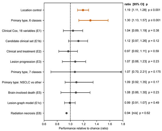
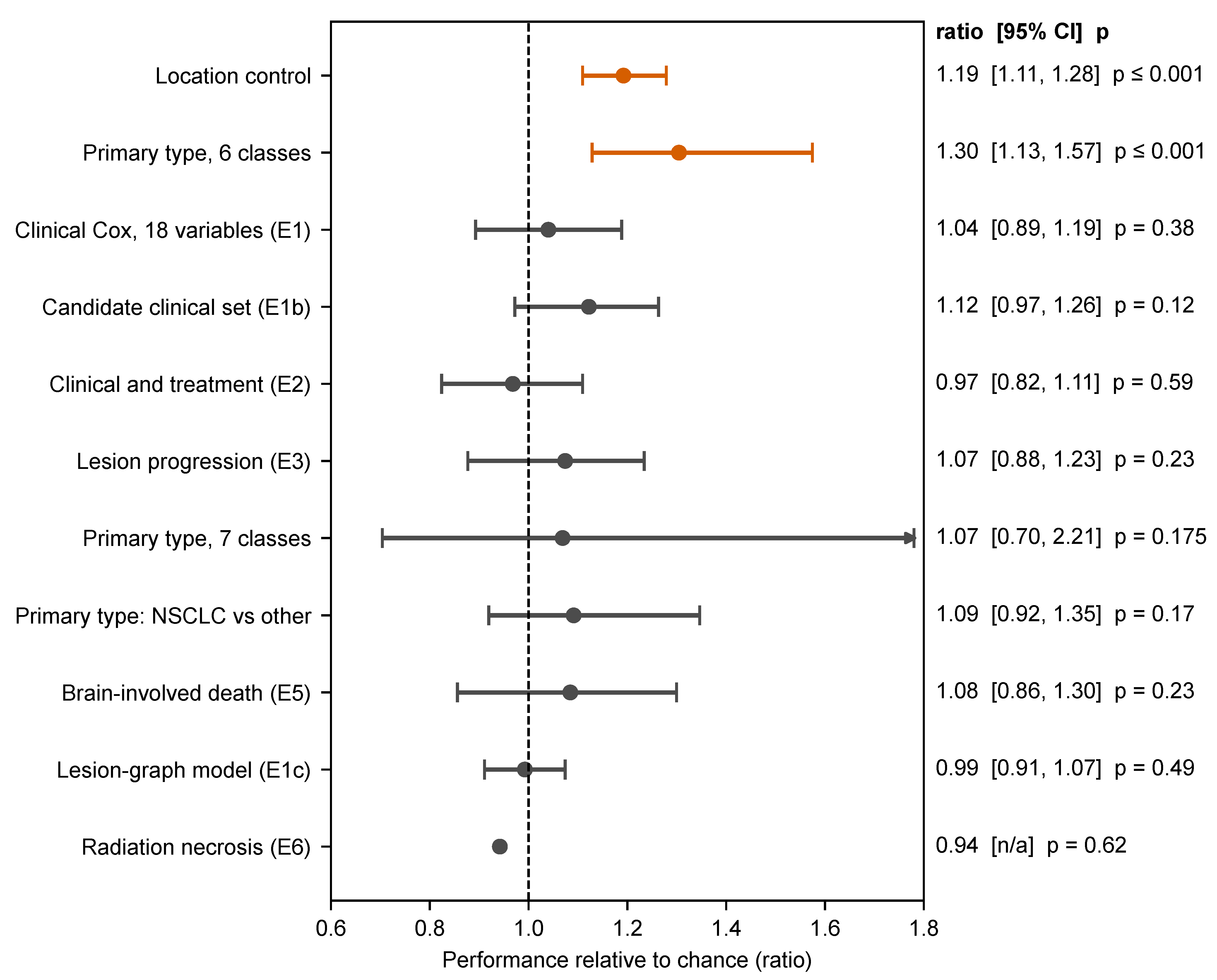
Primary tumor type was the only planned endpoint that remained significant after multiplicity correction: six-class balanced accuracy was 0.217 (95% CI 0.188–0.262; 1.30× chance; 1.38× with resampled embeddings), and its permutation p (≤0.001) was below both the Bonferroni threshold of 0.0063 and the stricter 0.0042. Recall exceeded chance for melanoma, NSCLC, gastrointestinal and breast primaries but not for renal or small-cell lung primaries (Supplement S5), and PyRadiomics features gave a similar result (balanced accuracy 0.26, 1.6× chance; 200 permutations, p ≤ 0.005). All other planned endpoints were null (Table 2; Figure 3). Survival C-indices ranged from 0.48 to 0.56. The graph model reached C = 0.496 ± 0.021 under nested validation (mean ± SD over ten training seeds; permutation null 0.496 ± 0.040, p = 0.49) and 0.549 ± 0.023 when the checkpoint was selected on the outer validation fold.
Figure 3.
Planned endpoints relative to chance (balanced-accuracy ratio or C-index/0.5). Bars are 95% intervals from a patient-level bootstrap of out-of-fold predictions (evaluation variance only); for E1, E1b, E2 and E3 the interval is translated so that it is anchored to the reported point estimate (Supplement S1). The exception is the graph model (E1c), where the interval is ±1.96 SD over ten training seeds; E6 has no interval. The upper end of the seven-class interval (2.21) lies beyond the axis. These intervals are not the bounds of Table 3. Orange: significant after Bonferroni correction for eight endpoints ( = 0.0063).
An exploratory linear Cox model on the mean lesion embedding per patient was not among the planned analyses. It reached C = 0.585 ± 0.016 (mean ± SD over 20 repeated 5-fold partitions, which reflects partition variability only; 0.571 ± 0.018 with a fully converged solver). A permutation test within primary tumor type gave p = 0.07 for one fixed partition, uncorrected for the number of variants examined (three embeddings, three penalties, two-fold constructions). The embeddings alone performed similarly to four clinical variables (0.54–0.56 in the planned analysis), and the risk score correlated only weakly with primary type ( ≤ 0.13), lesion count ( = ) and tumor volume ( = ). PyRadiomics features of the same lesions gave C = 0.53 (p = 0.29), and the combined feature set gave C = 0.45; the planned graph model, which uses the same embeddings, was at chance. We regard this as a weak, unconfirmed signal that depends on the representation; we did not determine why the linear and graph models differ.
In a single-partition analysis with embeddings from images resampled to 1.0 mm, the same type of model reached C = 0.63 (p = 0.005, the smallest value attainable with 200 permutations; Supplement S5), which exceeds the repeated-partition estimate for the original embeddings and illustrates how strongly such single estimates depend on the partition and on preprocessing.
3.3. GPA, Intracranial Burden and Mode of Death
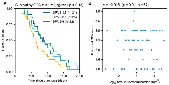
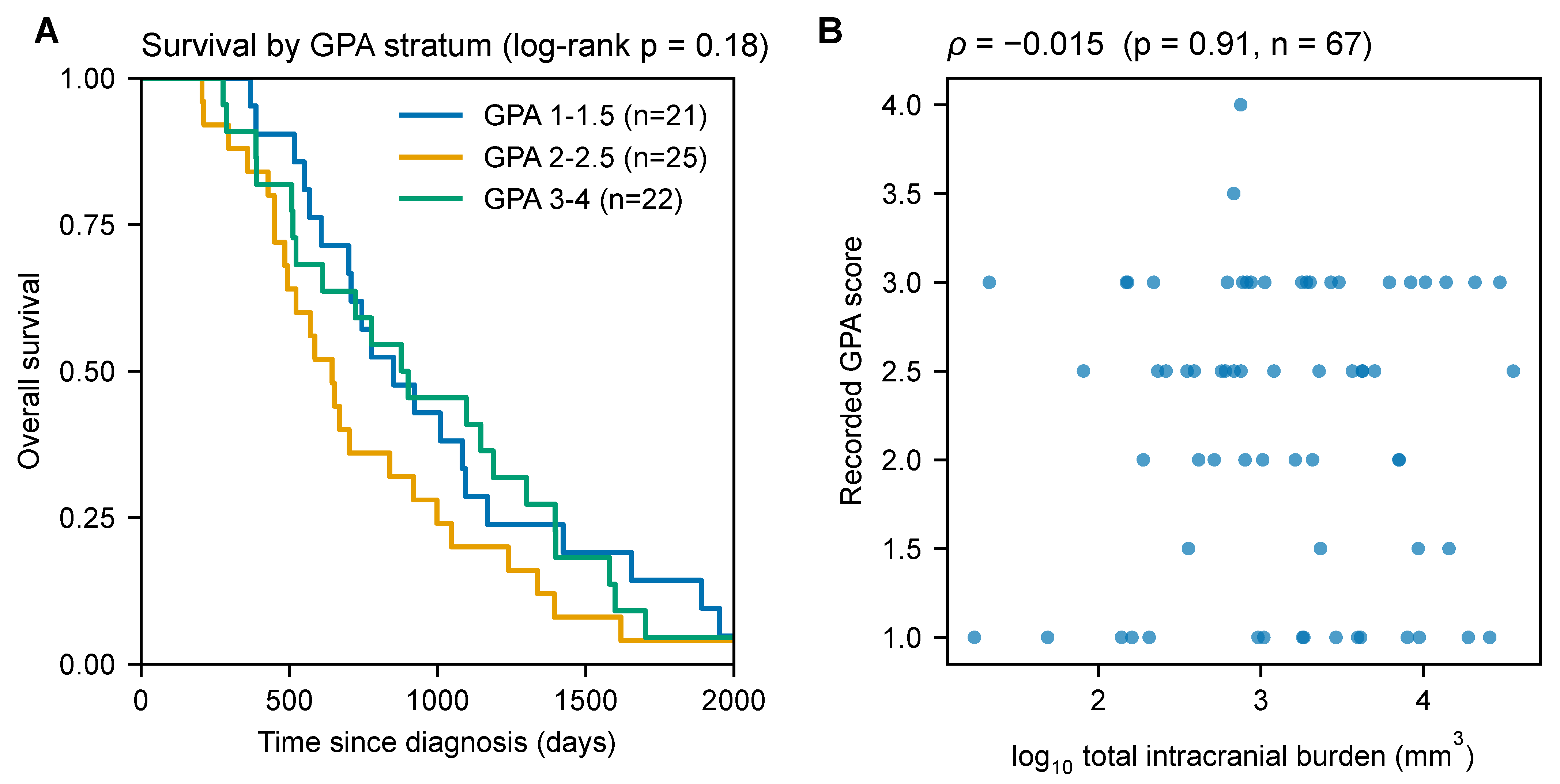
GPA did not significantly stratify survival in OpenBTAI (median survival 852, 645 and 878 days in the GPA 1–1.5, 2–2.5 and 3–4 strata; log-rank p = 0.18; Figure 4A), and the result was unchanged under four rules for choosing a patient’s GPA among conflicting lesion rows (p = 0.12–0.70); a median split gave p = 0.60. With 68 patients, all deceased, this is an absence of evidence and not evidence that GPA lacks prognostic value, which is established in much larger series [1]. GPA was uncorrelated with log intracranial burden ( = , p = 0.91) and lesion count ( = , p = 0.52) and correlated with age ( = , p = 0.018; Figure 4B).
Figure 4.
GPA and survival in OpenBTAI. (A) Kaplan–Meier curves by GPA stratum (n = 21, 25 and 22; median survival 852, 645 and 878 days; log-rank p = 0.18). (B) GPA versus total intracranial burden at first record ( = , p = 0.91, n = 67).
The radiomics read-out of GPA ( = 0.42, p = 0.006) persisted after removing age, lesion count and burden (partial 0.40–0.42; Appendix B), after permuting GPA only within primary tumor type (p = 0.006), and under the four GPA-row rules ( 0.35–0.45, p ≤ 0.02). Because KPS and extracranial status are not recorded, the read-out may reflect imaging correlates of unrecorded components, and a readable index is not necessarily a prognostic one.
Cause of death was usable for 68 patients: 52 (76%, 95% CI 65–85%) involved systemic illness (codes 2 or 3) and 8 (12%) isolated brain progression. This is a retrospective record without adjudication. Radiomics did not predict the recorded cause under any binary grouping of the four codes (all p ≥ 0.23; Benjamini–Hochberg [35] q = 1; Supplement S4), nor did clinical and treatment variables (cause-specific Cox, C = 0.48, p = 0.62).
3.4. Endpoint Definitions and Family-Wise Error
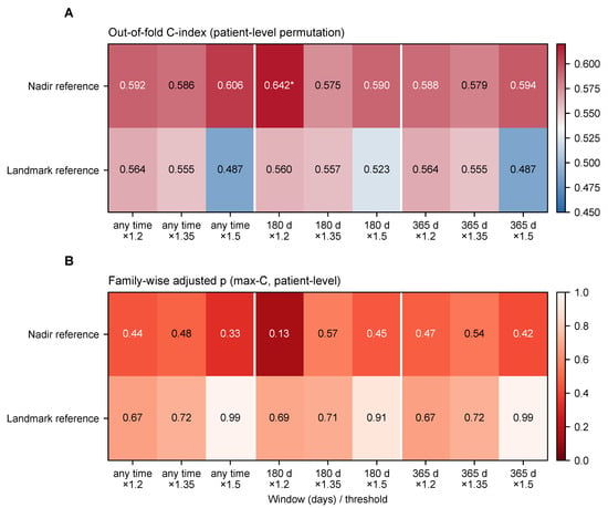
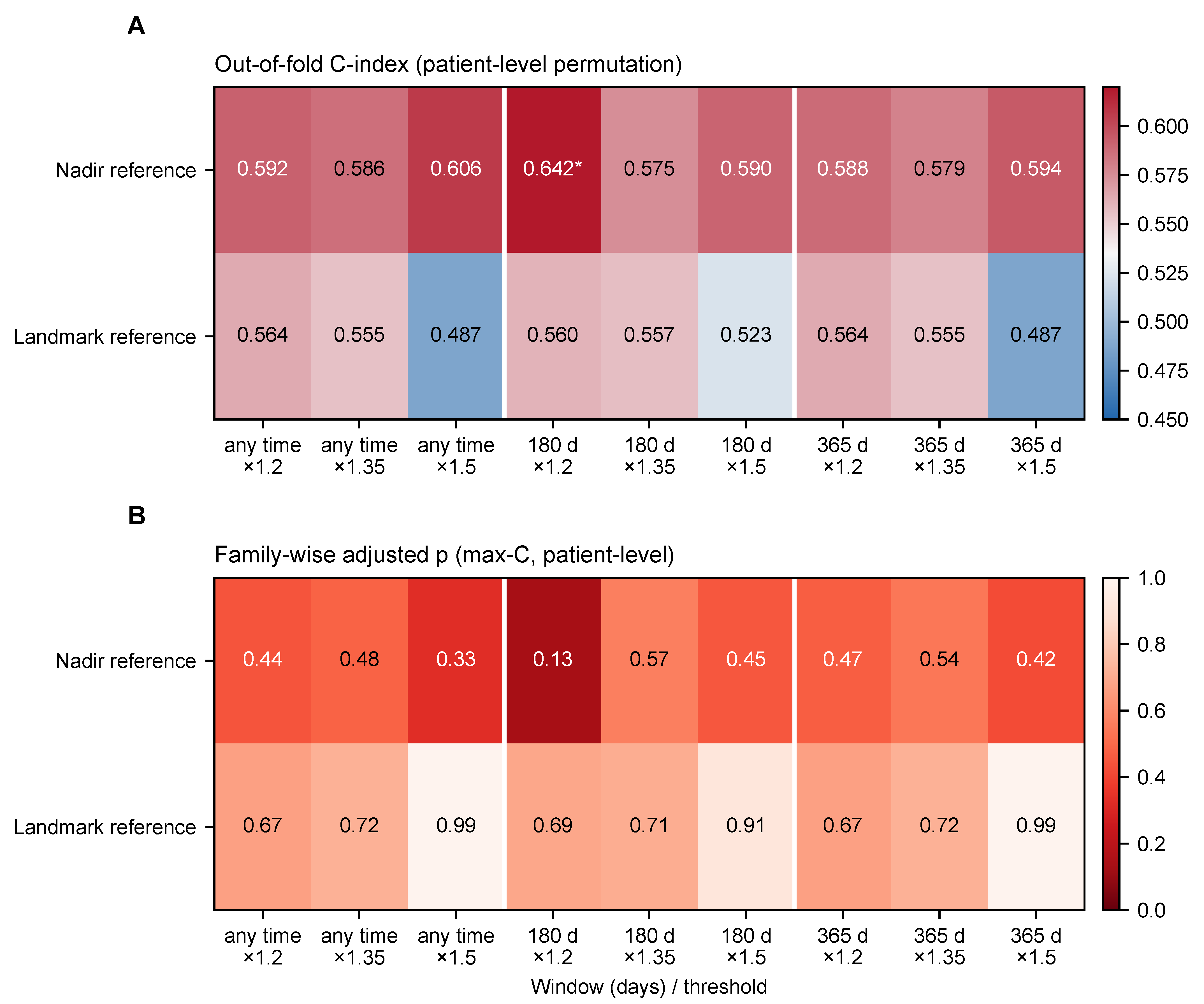
Across the 18 definitions of lesion progression in OpenBTAI, the cross-validated C-index ranged from 0.49 to 0.64. With patient-level permutation, one definition reached p < 0.05 (nadir reference, 180-day window, ×1.2; C = 0.64, p = 0.021); with lesion-level permutation, which ignores the clustering of lesions within patients, three did (smallest p = 0.009). After Westfall–Young correction, none were significant: the adjusted p of the best definition was 0.13 (max-C) or 0.16 (min-p) at patient level, and 0.07 or 0.10 at lesion level (Figure 5; Supplement S9). The three lesion-level hits all used the nadir reference, whose reference value comes from follow-up after the landmark; no definition in the landmark family, whose reference is fixed at the first post-treatment scan, approached significance (all p ≥ 0.11). Under the patient-level null, at least one of the 18 cells reached p < 0.05 in 31.5% of permutations and at least three in 11.7%, and the null C-indices of the cells were correlated (mean 0.40; range 0.13–0.77). A few nominally significant cells are, therefore, expected from noise, and the informative quantity is how far the best of 18 definitions falls from a family-wise threshold.
Figure 5.
Eighteen definitions of lesion progression. (A) Cross-validated C-index with patient-level permutation; an asterisk marks single-cell p < 0.05. (B) Westfall–Young adjusted p (max-C) at patient level; darker cells have smaller p. Rows: reference frame; columns: window (any time, 180 or 365 days) and growth threshold (×1.2, ×1.35 or ×1.5).
3.5. What the Null Results Can Exclude
Upper limits (observed C plus 1.96 SD) were 0.66 for the Yale candidate-variable Cox model, 0.54–0.58 for the graph model (0.537 with the seed SD, 0.575 with the permutation-null SD), 0.645 for OpenBTAI lesion progression and 0.585 for OpenBTAI survival (Table 3). They are rough guides and not exclusions, as the simulation shows.
Table 3.
Largest C-index compatible with the data for survival-type endpoints.
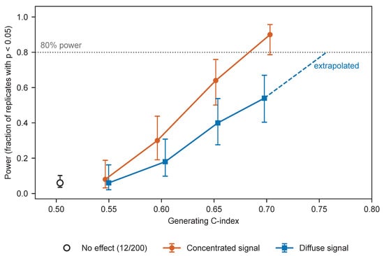
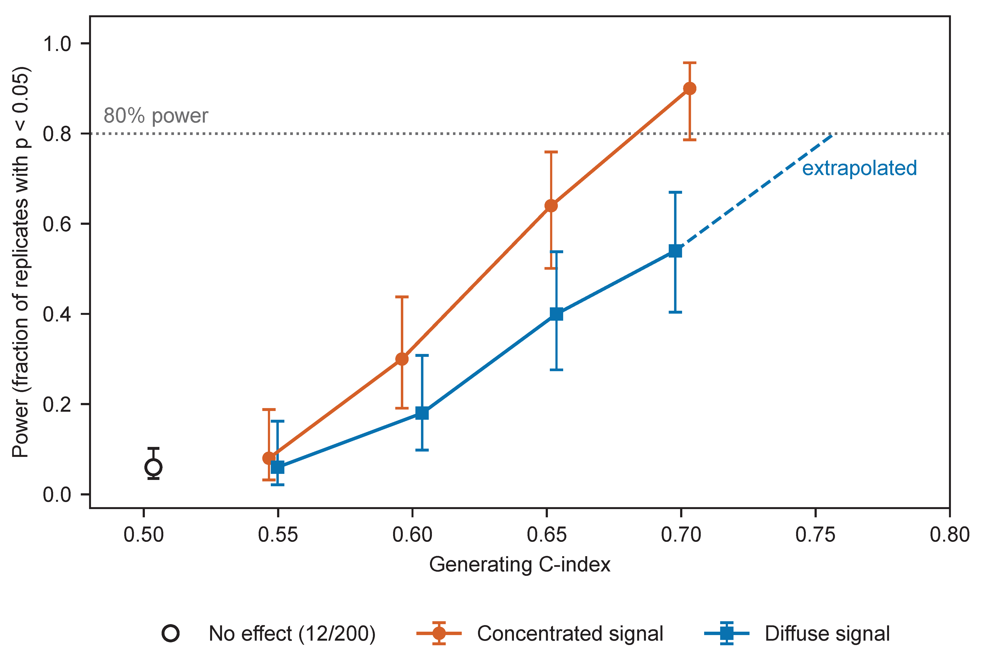
In the simulation, power at a generating C-index of about 0.60 was 0.30 when the signal lay in the leading principal components and 0.18 when it was dense across all 324 dimensions; at about 0.65 it was 0.64 and 0.40 (Figure 6). Eighty percent power was reached at a generating C-index of about 0.68 (concentrated) and, by extrapolation beyond the simulated grid, about 0.76 (dense). Cross-validated C-indices were 0.05–0.11 below the generating values. The SD under the alternative was on average 2% smaller than under the null (ratio 0.98; range 0.84–1.17), so the permutation-null approximation was not the main source of error; attenuation of the cross-validated C-index was. Under no effect, 12 of 200 replicates were significant (0.06; 95% CI 0.04–0.10). A check consisting of a positive control and a permutation test would, therefore, have declared an endpoint with a generating C-index of 0.65 not identifiable in 36–60% of replicates. Assuming that the SD scales with the inverse square root of the number of events, a difference of 0.10 in C-index would need roughly 235–490 events; this was not simulated directly. The simulation concerns the high-dimensional imaging-feature Cox model; low-dimensional clinical models lose less discrimination under cross-validation and are not covered.
Figure 6.
Power of the imaging survival pipeline in semi-synthetic data. Power versus generating C-index for a signal concentrated in the leading principal components and for a dense signal (Wilson 95% intervals; 50 replicates per setting); the open symbol is the no-effect setting (200 replicates). The dashed segment extrapolates beyond the simulated grid.
4. Discussion
4.1. Principal Findings
With lesion-centered embeddings, the pipeline recovered anatomical location and, modestly, primary tumor type; in OpenBTAI, it recovered quantities related to lesion size and the numeric GPA score; it did not recover brain age. Survival endpoints were null for clinical-variable and graph models, and an exploratory linear model on embeddings gave a weak signal (C ≈ 0.58) that PyRadiomics features did not reproduce. In simulation, the survival pipeline had 80% power only for generating C-indices of roughly 0.68–0.76. The results are, therefore, compatible with no signal and with moderate signals alike. An endpoint–cohort mismatch is one explanation among several; others are limited event counts, the absence of treatment information in Yale, outcome selection in OpenBTAI, and limited sensitivity of the imaging representations. Our data do not discriminate between them.
4.2. GPA
GPA was recoverable from imaging but did not significantly stratify survival and was uncorrelated with intracranial burden. A composite index dominated by components that are not brain-related could behave this way, but our data cannot show it: KPS and extracranial status are unrecorded, only deceased patients are included, and 68 patients give little power. Because OpenBTAI is selected on death, outcome-selection and spectrum bias [36] apply to the GPA result. The 76% share of deaths involving systemic illness is a descriptive statistic from a retrospective record with an unlabeled legend; the cause-of-death analysis is cause-specific and not a competing-risks analysis of a general population [37], and neither imaging features nor clinical variables predicted the recorded cause. The finding is a caution that a readable index is not a prognostic one, and a hypothesis for cohorts that record performance status and extracranial disease.
4.3. Lessons for Study Design
Four lessons emerged. First, extraction itself must be checked. Our first extraction centered patches on the wrong positions, yet the positive control was passed with both the misplaced and the corrected patches (balanced accuracy 0.604 and 0.596), so it could not reveal the error, and a brain-age association appeared that vanished once patches were lesion-centered. Second, power should be estimated by simulation with planted effects and not by extrapolating the permutation-null SD; cross-validated C-indices in a high-dimensional model lay 0.05–0.11 below the true discrimination. Third, endpoint definitions are a source of freedom: of 18 definitions, one to three reached nominal significance, and none survived family-wise correction. Fourth, single cross-validated numbers are unstable: fold construction moved one of our estimates by 0.05, and protocol choices such as the handling of censoring and the unit of scoring can move reported metrics by more than the effects sought (Appendix A). We, therefore, propose the following pre-flight checklist; apart from the simulation above, it has not been validated prospectively.
- Run positive controls of more than one kind, and state what each can and cannot certify.
- After feature extraction, assert that every crop contains its target, keep extraction logs and configuration, and check coordinate conventions visually on a few cases.
- Estimate power by simulation with planted effects in the real feature space, and read cross-validated metrics against the attenuation such simulations show.
- Fix the primary endpoint definition in writing; when several definitions are defensible, correct for the family.
- Report upper limits together with the power at those limits.
- Repeat cross-validation over partitions and seeds and report the spread.
- Check whether the cohort is selected on the outcome and which prognostic components and treatments are recorded.
- Plan for cohorts with several hundred events (our extrapolation: roughly 235–490 for a difference of 0.10 in C-index; not directly simulated).
4.4. Limitations
- OpenBTAI includes only deceased patients; survival distributions, GPA stratification and the mode-of-death result may not generalize.
- The sensitivity of the survival pipeline is limited. The simulation covers only the Yale feature space, two signal geometries and 50 replicates per setting; OpenBTAI and low-dimensional clinical models were not simulated.
- There was no external registration, and the planned endpoints rest on internal files; all exploratory analyses were designed after the first null results.
- Our first feature extraction contained a coordinate error, corrected during revision; no log of the first run was kept, and the cause was confirmed by reproducing the archived values.
- The controls recovered in OpenBTAI are size-related, and brain age was recovered in neither cohort.
- Treatment variables are not available in Yale, and KPS and extracranial status are not available in OpenBTAI; GPA and necrosis are recorded per lesion row.
- Cause of death is a retrospective record; the legend is unlabeled, one entry is truncated, and two patients carry conflicting codes.
- Both cohorts are single-institution sources with 74 and 75 deaths.
- Representations were limited to the encoder (native and resampled) and PyRadiomics in Yale and PyRadiomics in OpenBTAI, with light tuning only; foundation-model embeddings were not tested, and the three-channel encoder could not be applied to the single-sequence OpenBTAI data. Other segmentation backbones, such as an ensemble of residual U-Net and InceptionV4 modules for liver tumors [38], and multi-head-attention segmentation networks with radiomics-based survival ensembles for glioma [39], may yield different representations; neither was trained on brain metastasis MRI, and neither was tested here.
- The exploratory linear model was examined in many variants and is unconfirmed.
- The same-side edge feature of the graph model refers to the volume midline and not to the anatomical midline.
4.5. Future Work
Future work should test the GPA hypothesis in cohorts that record KPS and extracranial disease, evaluate foundation-model embeddings, and apply the checklist above, with an externally time-stamped registration, to cohorts with several hundred events.
5. Conclusions
On two public brain metastasis cohorts, lesion-centered imaging features recovered anatomical location and, modestly, primary tumor type; in OpenBTAI, radiomics recovered lesion size and the numeric value of a prognostic index. The survival models we evaluated were null, apart from an exploratory linear model with a weak and unconfirmed signal. Simulation shows that the survival pipeline would detect only strong effects, so these results do not exclude moderate ones, and they do not discriminate between an endpoint–cohort mismatch, limited event counts and limited sensitivity of the pipeline. In one cohort selected on death, GPA did not stratify survival, and most recorded deaths involved systemic illness, which we report descriptively. A coordinate error in our first feature extraction, found and corrected during revision, illustrates why extraction logs and visual checks belong in any pre-flight checklist.
Supplementary Materials
The following supporting information can be downloaded at https://www.mdpi.com/article/10.3390/jimaging12110560/s1. Supplement S1: implementation details, pretraining and segmentation quality (Figure S2), including the two versions of the clinical table, the positive-control label and the bootstrap intervals of Figure 3; Supplement S2: hyperparameter sensitivity and nested tuning; Supplement S3: the 46 exploratory tests with Benjamini–Hochberg correction; Supplement S4: cause of death, GPA row rules and necrosis definitions; Supplement S5: alternative representations and the six-class per-class recall; Supplement S6: sample-size flow (Figure S4); Supplement S7: first extraction, patch audit and centroid-axis audit (Figures S1 and S3); Supplement S8: additional OpenBTAI controls, including the three location axes; Supplement S9: the 18 endpoint definitions with patient-level and lesion-level p-values.
Author Contributions
Conceptualization, X.B. and J.W.; methodology, X.B. and J.W.; software, X.B.; validation, X.B., J.W. and X.Z.; formal analysis, X.B.; investigation, X.B. and J.W.; resources, X.Z. and J.W.; data curation, X.B.; writing—original draft preparation, X.B.; writing—review and editing, J.W., X.Z. and X.B.; visualization, X.B. and J.W.; supervision, J.W. and X.Z.; project administration, J.W.; funding acquisition, X.Z. All authors have read and agreed to the published version of the manuscript.
Funding
This research was funded by the National Key Research and Development Program of China, grant number 2024YFC2417802, and the Doctoral Research Start-up Foundation of Liaoning Province, grant number 2026-BS-0488.
Institutional Review Board Statement
Ethical review and approval were waived for this study due to it is a secondary analysis of publicly available, fully de-identified datasets (Yale/BraTS-MET, OpenBTAI/MOLAB, and UCSF-BMSR for encoder pretraining), and no new human subject data were collected. The original data collections were approved by their respective institutional review boards: Yale University (protocol 2000029055, approved 1 October 2020) [14] and the participating institutions of the OpenBTAI study [15].
Informed Consent Statement
Patient consent was waived due to the retrospective nature of the study and the exclusive use of publicly available, fully de-identified data. For Yale/BraTS-MET, the Yale University Institutional Review Board waived participant consent and approved open publication of the data [14]; in OpenBTAI/MOLAB, all included subjects are deceased [15].
Data Availability Statement
The evaluated cohorts are publicly accessible. Yale/BraTS-MET is available from The Cancer Imaging Archive (TCIA) as the Pretreat-MetsToBrain-Masks collection (https://doi.org/10.7937/6be1-r748; citation of the collection is required by TCIA). OpenBTAI/MOLAB is available from Figshare (https://doi.org/10.6084/m9.figshare.c.6194104.v1). The UCSF-BMSR dataset, used only for encoder pretraining, is available for non-commercial use under its own license (https://registry.opendata.aws/ucsf-bmsr/, accessed on 3 November 2026). Raw images and clinical tables are not redistributed by the authors and must be obtained from the original sources under their terms. All code, reproducibility protocols (including patient-grouped permutation test scripts, GNN nested cross-validation, and the 18-definition grid pipeline), and intermediate results are openly available at GitHub: https://github.com/lebron44768/BrainMet-Survival-Eval, accessed on 3 November 2026. The script for the external segmentation evaluation on the Yale cohort (evaluate_yale.py) is provided in the same repository (directory 06_external_dice/), together with the per-case Dice values it produced. The repository also contains the corrected and the first-extraction (misplaced-patch) embeddings with MD5 checksums, the centroid-axis audit, the revision analyses and the simulation code; the first-extraction embeddings are provided for transparency only and are not used in any result reported here.
Acknowledgments
The authors would like to thank the contributors of the Yale/BraTS-MET and OpenBTAI/MOLAB datasets for making their valuable clinical and imaging data publicly available. During the preparation of this manuscript, the authors used large language models for language translation and formatting, and an AI coding assistant to write and run parts of the analysis scripts during revision. The authors specified every analysis, checked every reported number against saved output, and take full responsibility for the content of this publication.
Conflicts of Interest
The authors declare no conflicts of interest.
Appendix A. Protocol-Element Sensitivity
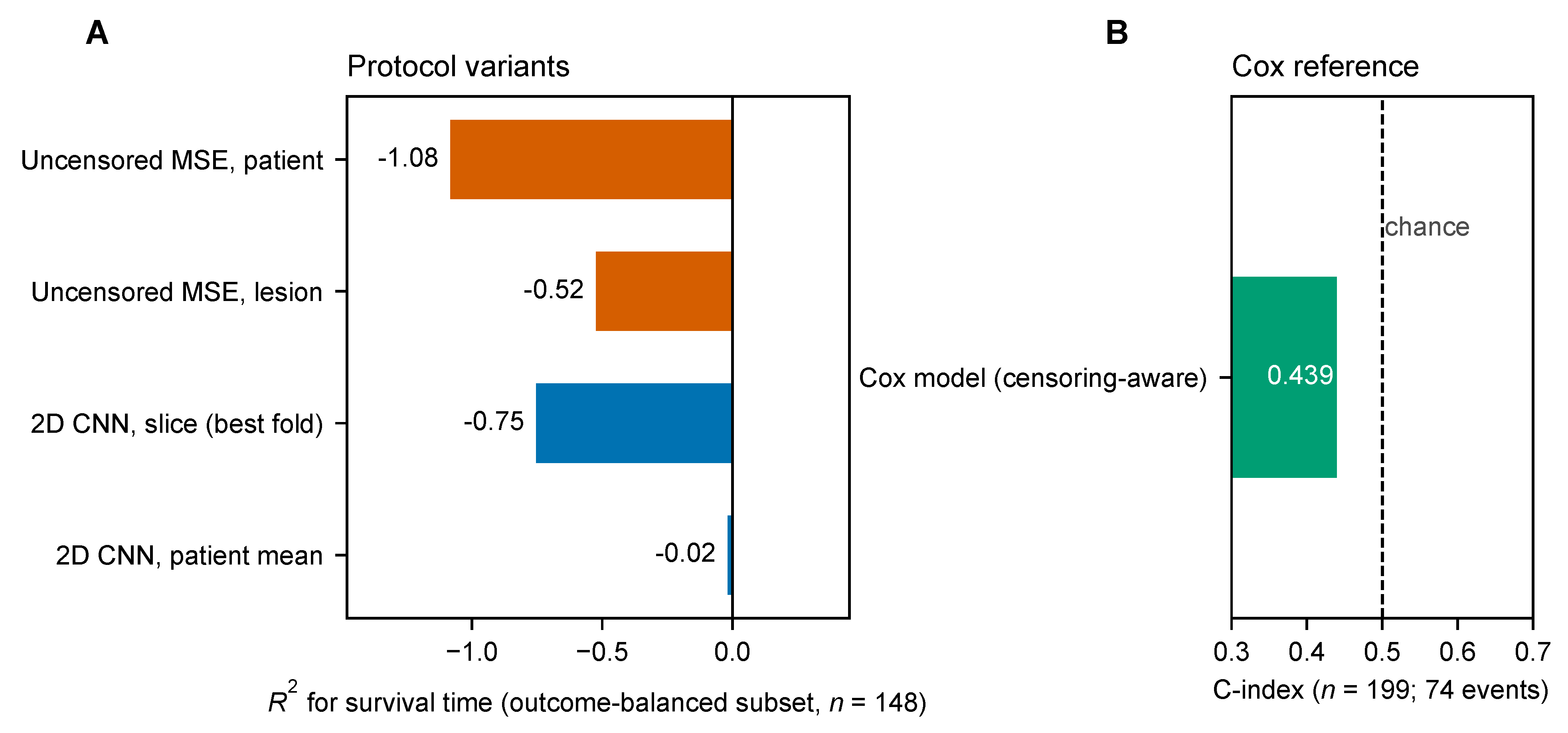
This analysis compared protocol variants on the Yale outcome-balanced subset () to show how design choices change the numerical value of a reported metric. The variants differed in censoring handling (with or without), scoring unit (patient level versus lesion-instance level), and the presence of a CNN branch. The analysis is not intended to reproduce any published result.
As shown in Figure A1, the uncensored MSE protocol, scored at the patient level, gave ; scored at the lesion-instance level instead, . A trained 2D CNN gave a best-fold slice-level , with a patient-level across-fold mean . These numbers illustrate how protocol elements (censoring treatment, scoring unit, and patient-level aggregation) substantially affect the numerical value of a reported metric. The censoring-aware reference in panel B uses all 199 patients rather than the 148-patient subset, because censored patients are retained in that analysis.
Figure A1.
Protocol-element sensitivity analysis. (A) for survival time of four protocol variants on the Yale outcome-balanced subset (): uncensored MSE at the patient and lesion-instance level, and a 2D CNN at the slice level (best fold) and at the patient level (mean over folds). (B) C-index of the censoring-aware Cox model on all 199 patients (74 events); the dashed line marks chance.
Appendix B. Additional Exploratory Data
Table A1 provides the full partial-correlation results for the GPA read-out under different covariate controls. Permutation p-values (1000 permutations; permutation of the GPA vector within primary tumor type, with the out-of-fold predictions held fixed) were computed for all controls.
Table A1.
GPA partial correlation under various measurable controls.
References
- Sperduto, P.W.; Kased, N.; Roberge, D.; Xu, Z.; Shanley, R.; Luo, X.; Sneed, P.K.; Chao, S.T.; Weil, R.J.; Suh, J.; et al. Summary report on the graded prognostic assessment: An accurate and facile diagnosis-specific tool to estimate survival for patients with brain metastases. J. Clin. Oncol. 2012, 30, 419–425. [Google Scholar] [CrossRef] [Scilit] [PubMed]
- Lipkova, J.; Chen, R.J.; Chen, B.; Lu, M.Y.; Barbieri, M.; Shao, D.; Vaidya, A.J.; Chen, C.; Zhuang, L.; Williamson, D.F.; et al. Artificial intelligence for multimodal data integration in oncology. Cancer Cell 2022, 40, 1095–1110. [Google Scholar] [CrossRef] [Scilit] [PubMed]
- Cui, C.; Yang, H.; Wang, Y.; Zhao, S.; Asad, Z.; Coburn, L.A.; Wilson, K.T.; Landman, B.A.; Huo, Y. Deep multimodal fusion of image and non-image data in disease diagnosis and prognosis: A review. Prog. Biomed. Eng. 2023, 5, 022001. [Google Scholar] [CrossRef] [Scilit] [PubMed]
- Kanakarajan, H.; De Baene, W.; Hanssens, P.; Sitskoorn, M. Predicting local control of brain metastases after stereotactic radiotherapy with clinical, radiomics and deep learning features. Radiat. Oncol. 2024, 19, 182. [Google Scholar] [CrossRef] [Scilit] [PubMed]
- Cho, S.J.; Cho, W.; Choi, D.; Sim, G.; Jeong, S.Y.; Baik, S.H.; Bae, Y.J.; Choi, B.S.; Kim, J.H.; Yoo, S.; et al. Prediction of treatment response after stereotactic radiosurgery of brain metastasis using deep learning and radiomics on longitudinal MRI data. Sci. Rep. 2024, 14, 11085. [Google Scholar] [CrossRef] [Scilit] [PubMed]
- Du, P.; Liu, X.; Shen, L.; Wu, X.; Chen, J.; Chen, L.; Cao, A.; Geng, D. Prediction of treatment response in patients with brain metastasis receiving stereotactic radiosurgery based on pre-treatment multimodal MRI radiomics and clinical risk factors: A machine learning model. Front. Oncol. 2023, 13, 1114194. [Google Scholar] [CrossRef] [Scilit] [PubMed]
- Keek, S.A.; Beuque, M.; Primakov, S.; Woodruff, H.C.; Chatterjee, A.; van Timmeren, J.E.; Vallières, M.; Hendriks, L.E.L.; Kraft, J.; Andratschke, N.; et al. Predicting Adverse Radiation Effects in Brain Tumors After Stereotactic Radiotherapy With Deep Learning and Handcrafted Radiomics. Front. Oncol. 2022, 12, 920393. [Google Scholar] [CrossRef] [Scilit] [PubMed]
- Zhao, J.; Vaios, E.; Calabrese, E.; Yang, Z.; Robertson, S.; Ginn, J.; Lu, K.; Yin, F.-F.; Reitman, Z.; Kirkpatrick, J.; et al. A Radiogenomic Deep Ensemble Learning Model for Identifying Radionecrosis Following Brain Metastases (BM) Stereotactic Radiosurgery in Patients with Non-small Cell Lung Cancer BM. Adv. Radiat. Oncol. 2025, 10, 101826. [Google Scholar] [CrossRef] [Scilit] [PubMed]
- Li, Y.; Lv, X.; Chen, C.; Yu, R.; Wang, B.; Wang, D.; Hou, D. A deep learning model integrating multisequence MRI to predict EGFR mutation subtype in brain metastases from non-small cell lung cancer. Eur. Radiol. Exp. 2024, 8, 2. [Google Scholar] [CrossRef] [Scilit] [PubMed]
- Habibi, M.A.; Rashidi, F.; Habibzadeh, A.; Mehrtabar, E.; Arshadi, M.R.; Mirjani, M.S. Prediction of the treatment response and local failure of patients with brain metastasis treated with stereotactic radiosurgery using machine learning: A systematic review and meta-analysis. Neurosurg. Rev. 2024, 47, 199. [Google Scholar] [CrossRef] [Scilit] [PubMed]
- Desai, S.P.; Hori, Y.S.; Kattaa, A.H.; Izhar, M.; Lam, F.C.; Reesh, D.A.; Tayag, A.; Ustrzynski, L.; Emrich, S.C.; Gu, X.; et al. Artificial intelligence (AI) uses in stereotactic radiosurgery (SRS): Outcome prediction with brain metastasis (BM)—A systematic review. J. Clin. Neurosci. 2026, 145, 111854. [Google Scholar] [CrossRef] [Scilit] [PubMed]
- Morelli, I.; Banini, M.; Greto, D.; Visani, L.; Garlatti, P.; Loi, M.; Aquilano, M.; Valzano, M.; Salvestrini, V.; Bertini, N.; et al. Integrating Radiomics and Artificial Intelligence (AI) in Stereotactic Body Radiotherapy (SBRT)/Stereotactic Radiosurgery (SRS): Predictive Tools for Tailored Cancer Care. Cancers 2025, 17, 2906. [Google Scholar] [CrossRef] [Scilit] [PubMed]
- Kim, H.Y.; Cho, S.J.; Sunwoo, L.; Baik, S.H.; Bae, Y.J.; Choi, B.S.; Jung, C.; Kim, J.H. Classification of true progression after radiotherapy of brain metastasis on MRI using artificial intelligence: A systematic review and meta-analysis. Neuro-Oncol. Adv. 2021, 3, vdab080. [Google Scholar] [CrossRef] [Scilit] [PubMed]
- Ramakrishnan, D.; Jekel, L.; Chadha, S.; Janas, A.; Moy, H.; Maleki, N.; Sala, M.; Kaur, M.; Petersen, G.C.; Merkaj, S.; et al. A Large Open Access Dataset of Brain Metastasis 3D Segmentations on MRI with Clinical and Imaging Information. Sci. Data 2024, 11, 254. [Google Scholar] [CrossRef] [Scilit] [PubMed]
- Ocaña-Tienda, B.; Pérez-Beteta, J.; Villanueva-García, J.D.; Romero-Rosales, J.A.; Molina-García, D.; Suter, Y.; Asenjo, B.; Albillo, D.; Ortiz de Mendivil, A.; Pérez-Romasanta, L.A.; et al. A Comprehensive Dataset of Annotated Brain Metastasis MR Images with Clinical and Radiomic Data. Sci. Data 2023, 10, 208. [Google Scholar] [CrossRef] [Scilit] [PubMed]
- Volovăţ, C.C.; Buzea, C.G.; Boboc, D.-I.; Ostafe, M.-R.; Agop, M.; Ochiuz, L.; Burlea, Ş.L.; Rusu, D.I.; Bujor, L.; Iancu, D.T.; et al. Hybrid Deep Learning for Survival Prediction in Brain Metastases Using Multimodal MRI and Clinical Data. Diagnostics 2025, 15, 1242. [Google Scholar] [CrossRef] [Scilit] [PubMed]
- Saeed, N.; Sobirov, I.; Majzoub, R.A.; Yaqub, M. TMSS: An End-to-End Transformer-based Multimodal Network for Segmentation and Survival Prediction. arXiv 2022, arXiv:2209.05036. [Google Scholar] [CrossRef] [Scilit]
- Gomaa, A.; Huang, Y.; Hagag, A.; Schmitter, C.; Höfler, D.; Weissmann, T.; Breininger, K.; Schmidt, M.; Stritzelberger, J.; Delev, D.; et al. Comprehensive multimodal deep learning survival prediction enabled by a transformer architecture: A multicenter study in glioblastoma. Neuro-Oncol. Adv. 2024, 6, vdae122. [Google Scholar] [CrossRef] [Scilit] [PubMed]
- Kim, S.Y. GNN-surv: Discrete-Time Survival Prediction Using Graph Neural Networks. Bioengineering 2023, 10, 1046. [Google Scholar] [CrossRef] [Scilit] [PubMed]
- Alzoubi, I.; Zhang, L.; Zheng, Y.; Loh, C.; Wang, X.; Graeber, M.B. PathoGraph: An Attention-Based Graph Neural Network Capable of Prognostication Based on CD276 Labelling of Malignant Glioma Cells. Cancers 2024, 16, 750. [Google Scholar] [CrossRef] [Scilit] [PubMed]
- Kazmierski, M.; Haibe-Kains, B. Lymph Node Graph Neural Networks for Cancer Metastasis Prediction. arXiv 2021, arXiv:2106.01711. [Google Scholar] [CrossRef] [Scilit]
- Campanella, G.; Häggström, I.; Kook, L.; Hothorn, T.; Fuchs, T.J. A Flexible Deep Learning Framework for Survival Analysis with Medical Data. In Proceedings of the Medical Image Computing and Computer Assisted Intervention–MICCAI 2025; Gee, J.C., Alexander, D.C., Hong, J., Iglesias, J.E., Sudre, C.H., Venkataraman, A., Golland, P., Kim, J.H., Park, J., Eds.; Springer Nature: Cham, Switzerland, 2026; Volume 15974, pp. 3–13. [Google Scholar] [CrossRef] [Scilit]
- Collins, G.S.; Moons, K.G.M.; Dhiman, P.; Riley, R.D.; Beam, A.L.; Van Calster, B.; Ghassemi, M.; Liu, X.; Reitsma, J.B.; van Smeden, M.; et al. TRIPOD+AI statement: Updated guidance for reporting clinical prediction models that use regression or machine learning methods. BMJ 2024, 385, e078378. [Google Scholar] [CrossRef] [Scilit] [PubMed]
- Wolff, R.F.; Moons, K.G.M.; Riley, R.D.; Whiting, P.F.; Westwood, M.; Collins, G.S.; Reitsma, J.B.; Kleijnen, J.; Mallett, S. PROBAST: A Tool to Assess the Risk of Bias and Applicability of Prediction Model Studies. Ann. Intern. Med. 2019, 170, 51–58. [Google Scholar] [CrossRef] [Scilit] [PubMed]
- Lambin, P.; Leijenaar, R.T.H.; Deist, T.M.; Peerlings, J.; de Jong, E.E.C.; van Timmeren, J.; Sanduleanu, S.; Larue, R.T.H.M.; Even, A.J.G.; Jochems, A.; et al. Radiomics: The bridge between medical imaging and personalized medicine. Nat. Rev. Clin. Oncol. 2017, 14, 749–762. [Google Scholar] [CrossRef] [Scilit] [PubMed]
- Mongan, J.; Moy, L.; Kahn, C.E., Jr. Checklist for Artificial Intelligence in Medical Imaging (CLAIM): A Guide for Authors and Reviewers. Radiol. Artif. Intell. 2020, 2, e200029. [Google Scholar] [CrossRef] [Scilit] [PubMed]
- Varma, S.; Simon, R. Bias in error estimation when using cross-validation for model selection. BMC Bioinform. 2006, 7, 91. [Google Scholar] [CrossRef] [Scilit] [PubMed]
- Cawley, G.C.; Talbot, N.L.C. On over-fitting in model selection and subsequent selection bias in performance evaluation. J. Mach. Learn. Res. 2010, 11, 2079–2107. [Google Scholar]
- Isensee, F.; Jaeger, P.F.; Kohl, S.A.A.; Petersen, J.; Maier-Hein, K.H. nnU-Net: A self-configuring method for deep learning-based biomedical image segmentation. Nat. Methods 2021, 18, 203–211. [Google Scholar] [CrossRef] [Scilit] [PubMed]
- Rudie, J.D.; Saluja, R.; Weiss, D.A.; Nedelec, P.; Calabrese, E.; Colby, J.B.; Laguna, B.; Mongan, J.; Braunstein, S.; Hess, C.P.; et al. The University of California San Francisco Brain Metastases Stereotactic Radiosurgery (UCSF-BMSR) MRI Dataset. Radiol. Artif. Intell. 2024, 6, e230126. [Google Scholar] [CrossRef] [Scilit] [PubMed]
- Westfall, P.H.; Young, S.S. Resampling-Based Multiple Testing: Examples and Methods for p-Value Adjustment; Wiley: New York, NY, USA, 1993. [Google Scholar]
- Lin, N.U.; Lee, E.Q.; Aoyama, H.; Barani, I.J.; Barboriak, D.P.; Baumert, B.G.; Bendszus, M.; Brown, P.D.; Camidge, D.R.; Chang, S.M.; et al. Response assessment criteria for brain metastases: Proposal from the RANO group. Lancet Oncol. 2015, 16, e270–e278. [Google Scholar] [CrossRef] [Scilit] [PubMed]
- Eisenhauer, E.A.; Therasse, P.; Bogaerts, J.; Schwartz, L.H.; Sargent, D.; Ford, R.; Dancey, J.; Arbuck, S.; Gwyther, S.; Mooney, M.; et al. New response evaluation criteria in solid tumours: Revised RECIST guideline (version 1.1). Eur. J. Cancer 2009, 45, 228–247. [Google Scholar] [CrossRef] [Scilit] [PubMed]
- Cole, J.H.; Franke, K. Predicting Age Using Neuroimaging: Innovative Brain Ageing Biomarkers. Trends Neurosci. 2017, 40, 681–690. [Google Scholar] [CrossRef] [Scilit] [PubMed]
- Benjamini, Y.; Hochberg, Y. Controlling the false discovery rate: A practical and powerful approach to multiple testing. J. R. Stat. Soc. Ser. B 1995, 57, 289–300. [Google Scholar] [CrossRef] [Scilit]
- Ransohoff, D.F.; Feinstein, A.R. Problems of spectrum and bias in evaluating the efficacy of diagnostic tests. N. Engl. J. Med. 1978, 299, 926–930. [Google Scholar] [CrossRef] [Scilit] [PubMed]
- Austin, P.C.; Lee, D.S.; Fine, J.P. Introduction to the Analysis of Survival Data in the Presence of Competing Risks. Circulation 2016, 133, 601–609. [Google Scholar] [CrossRef] [Scilit] [PubMed]
- Rahman, H.; Ben Aoun, N.; Naik Bukht, T.F.; Ahmad, S.; Tadeusiewicz, R.; Pławiak, P.; Hammad, M. Automatic liver tumor segmentation of CT and MRI volumes using ensemble ResUNet-InceptionV4 model. Inf. Sci. 2025, 704, 121966. [Google Scholar] [CrossRef] [Scilit]
- Rasool, N.; Bhat, J.I.; Ben Aoun, N.; Alharthi, A.; Wani, N.A.; Chopra, V.; Anwar, M.S. ResMHA-Net: Enhancing Glioma Segmentation and Survival Prediction Using a Novel Deep Learning Framework. Comput. Mater. Contin. 2024, 81, 887–911. [Google Scholar] [CrossRef] [Scilit]

Disclaimer/Publisher’s Note: The statements, opinions and data contained in all publications are solely those of the individual author(s) and contributor(s) and not of MDPI and/or the editor(s). MDPI and/or the editor(s) disclaim responsibility for any injury to people or property resulting from any ideas, methods, instructions or products referred to in the content. |
© 2026 by the authors. Licensee MDPI, Basel, Switzerland. This article is an open access article distributed under the terms and conditions of the Creative Commons Attribution (CC BY) license.