


Abstract
Fault diagnosis in grid-connected grid-forming hybrid energy storage station (GFM-HESS) systems is challenging because fault transients are jointly affected by converter control dynamics, multi-source electrical couplings, operating-condition variations, and measurement noise. To address these characteristics, this paper proposes a virtual synchronous generator (VSG)-constrained physics-informed heterogeneous temporal graph neural network (VSG-PI-HTGNN) for multi-class fault diagnosis. Based on VSG control characteristics and electrical relationships, 18-dimensional node-level features and eight-dimensional global physical features are constructed from ten monitored signals. These signals are further represented as a heterogeneous graph with five node types and eight predefined relation types, while node-type-specific transformations, heterogeneous graph convolution, learnable relation-scaling factors, and a primary–auxiliary dual-output framework are integrated for feature learning. A MATLAB/Simulink electromagnetic transient model is established to generate 3200 samples covering normal operation and nine fault conditions. At a signal-to-noise ratio (SNR) of 18 dB, the proposed model achieves 97.25% test accuracy and a macro-F1 score of 0.9727. Ablation results show that removing all physical information reduces the accuracy to 89.83%, while, under the unified experimental setting, the proposed model obtains higher values of the reported diagnostic metrics than the seven considered benchmark methods. Further evaluations show that the accuracy remains between 95.50% and 98.75% across SNR levels of 10–30 dB and reaches 95.38% with only 20% of the training data. Validation using an independently acquired hardware-in-the-loop (HIL) dataset further yields 92.75% accuracy and a macro-F1 score of 0.9282. Overall, these results indicate that the proposed method provides favorable diagnostic accuracy, noise robustness, data efficiency under limited-sample conditions, and simulation-to-HIL transferability under the evaluated conditions.
1. Introduction
With the increasing penetration of inverter-based renewable generation and the reduction in synchronous inertia, grid-forming converters (GFMCs) have received growing attention because of their capability to establish voltage and frequency references and provide inertia-like responses [1]. Hybrid energy storage systems (HESSs) combine storage technologies with complementary power, energy, and response characteristics and can provide flexible regulation over different time scales [2]. The integration of grid-forming control with HESSs provides a possible means of coordinating multiple storage units while maintaining grid-supporting capability [3]. As the application of grid-forming hybrid energy storage stations (GFM-HESSs) develops, fault diagnosis becomes relevant for identifying abnormal operating states and fault types and for supporting subsequent fault analysis and operational assessment.
Fault diagnosis of a GFM-HESS presents characteristics associated with converter control and multi-component coupling. The fault current of a GFMC is constrained by semiconductor current capability and is influenced by grid disturbances, control parameters, current-limiting actions, and grid conditions [4,5]. Moreover, a GFM-HESS involves interactions among multiple storage units, the DC bus, the GFMC, and the external grid. Therefore, DC-bus voltage, three-phase voltages and currents, frequency, and active/reactive power may exhibit coupled transient responses rather than independent variations. Diagnostic methods based mainly on individual signal amplitudes, fixed criteria, or directly learned raw time-series features may make limited use of these physical relationships, particularly under noisy or varying operating conditions [6]. Incorporating physical information and inter-variable relationships into data-driven models may therefore provide a useful direction for GFM-HESS fault classification.
Existing studies have explored grid-forming inverter fault detection using DC-link information, observer residuals, and adaptive thresholds [7,8,9]. For multi-class fault diagnosis, Mulinka et al. [10] develop a digital-twin framework for VSG-controlled grid-connected inverters and employ Bayesian optimization to improve diagnostic performance under limited data. The framework is subsequently extended by considering data quality and decision reliability [11]. These studies indicate that converter models, control information, and multi-source measurements can contribute to fault diagnosis. However, different electrical variables are generally treated as diagnostic inputs or model outputs, while their control-dependent relationships are not always explicitly represented.
Physics-informed learning provides another approach for incorporating prior knowledge into data-driven models. Ngo et al. [12] integrate physical equations with graph learning for power-system state estimation. Jabbari Zideh and Solanki [13] incorporate physical relationships into a convolutional autoencoder for anomaly detection, while Falas et al. [14] introduce physical constraints into neural-network-based state estimation. Related studies have shown the potential of physics-informed learning for improving model consistency and robustness [15]. Nevertheless, these methods mainly introduce circuit equations, state relationships, or physical constraints into estimation and anomaly-detection tasks. The use of VSG control dynamics and GFM-HESS-specific electrical relationships to construct class-discriminative fault features remains relatively limited.
Graph neural networks (GNNs) provide a suitable framework for representing relationships among multiple measurements or system components. Nguyen et al. [16] develop a spatial-temporal recurrent GNN for fault diagnosis in distribution systems, while Ngo et al. [17] employ deep graph learning to integrate electrical measurements and network information for fault detection and identification. These studies demonstrate the potential of graph-based information propagation for incorporating spatial and structural dependencies. However, most power-system GNNs are constructed primarily according to electrical-network topology and generally represent buses, branches, or similar entities using relatively uniform node and edge definitions.
Heterogeneous graph learning extends this framework by distinguishing different node categories and relation types. Chanda and Soltani [18] develop a heterogeneous graph-based multi-task model for fault-event diagnosis in smart grids. Heterogeneous graph representations have also been investigated for adaptive machine fault diagnosis [19], multi-sensor fusion in AC motor fault diagnosis [20], and multi-modal rotating-machinery fault diagnosis [21]. Liu et al. [22] further combine heterogeneous graph modeling with cross-modal information fusion for grid fault diagnosis. These studies suggest that heterogeneous graphs can provide a flexible representation of different data sources and relationships. Nevertheless, existing applications mainly focus on network topology, equipment states, or multimodal information, whereas heterogeneous relationships derived from VSG control and DC/AC electrical coupling in a GFM-HESS have received comparatively less attention.
Representative methods are compared in Table 1.
Table 1.
VSG-based node-level features.
Overall, existing studies provide useful foundations for physics-informed diagnosis and graph-based relational modeling. However, two aspects remain worthy of further investigation for GFM-HESS fault diagnosis. First, physical information in existing diagnostic or physics-informed models is commonly introduced as detection criteria, state equations, or model constraints, whereas the control-dependent transient characteristics of VSG-controlled GFMCs have not been sufficiently incorporated into multi-level fault feature representations. Second, existing graph-based methods mainly define graph structures according to network topology or general data associations, while the heterogeneous relationships among DC-bus voltage, three-phase voltages and currents, frequency, and power in a GFM-HESS remain relatively less explored. Combining physics-informed feature construction with heterogeneous relation modeling may therefore provide a suitable representation of GFM-HESS fault transients.
To address these issues, this paper develops a VSG-constrained Physics-Informed Heterogeneous Temporal Graph Neural Network (VSG-PI-HTGNN) for multi-class fault diagnosis of a grid-connected GFM-HESS. The main contributions are summarized as follows:
- (1)
- A dual-level physics-informed feature representation is developed based on the transient characteristics of monitored electrical variables and the control relationships of the GFMC. Unlike approaches that rely primarily on raw signals or general statistical descriptors, the proposed representation incorporates node-level transient information together with system-level physical information derived from VSG dynamics, sequence components, DC-bus behavior, and power relationships, thereby introducing control-related prior knowledge into fault feature construction.
- (2)
- A measurement-oriented heterogeneous physical graph is constructed to describe the coupling relationships among different electrical variables. Different measurement categories and control/electrical relations are represented using different node and edge types rather than being treated uniformly. Node-type-specific transformations and learnable relation-scaling factors further allow the contributions of different predefined relation types to be adjusted during graph information propagation.
- (3)
- A primary–auxiliary multi-task learning framework is combined with the physics-informed heterogeneous graph to improve the representation of different fault classes under noisy and limited-sample conditions. The proposed model is evaluated through simulation-based testing, noise-robustness and limited-sample analyses, component-level comparisons, and Sim-to-HIL transferability validation, providing complementary evaluations of diagnostic performance under different test conditions.
2. VSG-PI-HTGNN Model
2.1. Dual-Branch Physical Feature Extraction
2.1.1. VSG-Based Node-Level Feature Extraction
The core principle of the VSG control mechanism is to incorporate the rotor motion equation and the active power–frequency droop characteristic of a synchronous generator into inverter control. This enables the GFMC to emulate the inertia and damping behavior of a conventional synchronous generator, thereby providing frequency support to the grid. The fundamental swing equation can be expressed as:
where and denote the active power reference and the actual active power of the GFMC at time t, respectively. is the moment of inertia of the GFMC at time t. is the angular frequency deviation. and represent the rotational angular speed and the rated angular speed of the GFMC at time t, respectively. is the damping coefficient of the GFMC.
In addition to the aforementioned active power–frequency control loop, the VSG control strategy also includes the reactive power–voltage control loop and the inner voltage and current control loops. These control loops jointly affect the voltage, current, frequency, and power outputs of the GFMC. Consequently, different fault conditions induce distinct variations in the multi-source measurement signals, while the VSG control loops further influence the transient evolution of these signals during the fault process.
Based on the above analysis, the ten multi-source measurement signals in each data sample are not simply treated as homogeneous time-series inputs. Instead, according to their physical attributes, they are categorized into five node types: DC, current, voltage, frequency, and power nodes. For each node signal, 18-dimensional statistical features are extracted from the steady-state and transient windows to characterize its local dynamic variations during fault transients. The first six dimensions are basic statistical features shared by all node types, whereas the remaining twelve dimensions are type-specific features designed according to the VSG-related physical characteristics of each node type. The detailed feature definitions are provided in Table 2.
Table 2.
VSG-based node-level features.
Let the signal sequence of node v within the feature-extraction window be . The local features are defined as follows:
where Nw denotes the number of sampling points within the window. denotes the signal value of node v at the k-th sampling point. , , and denote the mean, standard deviation, peak value, and root-mean-square (RMS) value, respectively, of the signal within the feature-extraction window. By applying the steady-state and transient windows separately, the steady-state mean, transient mean, steady-state standard deviation, and transient standard deviation are obtained.
The local feature is defined as:
where denotes the normalized fluctuation feature of the signal at node v. denotes the rated value corresponding to . ε is a small positive constant introduced to avoid division by zero.
The local feature is defined as:
where denotes the normalized range feature of the signal at node v; and denote the maximum and minimum values, respectively, of within the feature-extraction window.
The local feature is defined as:
where denotes the abnormal-value ratio of the signal at node v within the feature-extraction window; for current and voltage nodes, it corresponds to the negative-sequence ratio. and denote the positive- and negative-sequence components, respectively, of the three-phase currents or voltages at the corresponding current or voltage node. denote the phase-A, phase-B, and phase-C signal values, respectively. is the indicator function, which equals 1 when the specified condition is satisfied and 0 otherwise. denotes the threshold for abnormality detection.
The local feature is defined as:
where denotes the limit-exceedance ratio of the signal at node v within the feature-extraction window. and denote the upper and lower safety limits, respectively, of .
The local features are defined as follows:
where , , and denote the skewness, kurtosis, and mean absolute difference, respectively, of the signal at node v within the feature-extraction window.
The local features are defined as follows:
where denotes the relative difference between the mean values of the first and second halves of the same feature-extraction window for the signal at node v, thereby characterizing the trend shift during the fault process. and denote the corresponding mean values of the first and second halves for the signal at node v, respectively. denotes the relative difference between the mean values of in the steady-state and transient feature-extraction windows, thereby characterizing the magnitude shift induced by the fault. and denote the mean values of in the steady-state and transient windows, respectively.
The local features are defined as follows:
where and denote the active-power and reactive-power deviation indices, respectively, of the GFMC output. and denote the reference values of the GFMC active and reactive power, respectively, within the feature-extraction window. and denote their corresponding mean values within the window, calculated in the same manner as in Equation (2). denotes the degree of correlation between the variation trends of active and reactive power within the feature-extraction window and characterizes the coupling between the active- and reactive-power responses. and denote the GFMC active and reactive power outputs, respectively, within the feature-extraction window.
2.1.2. Global Physical Feature Extraction
In addition to the node-level features, an 8-dimensional global physical feature vector is further extracted to characterize the overall operating state of the GFM-HESS. These features are constructed based on Kirchhoff’s laws, symmetrical component analysis, and the VSG swing equation, enabling the characterization of circuit constraint relationships and control dynamic responses at the system level.
Unlike node-level features, which focus on describing the variation characteristics of individual node signals, global physical features emphasize the overall physical consistency of the system. They can be incorporated into the model as physics-informed prior knowledge, providing supplementary constraints for subsequent feature learning. The detailed feature configuration is presented in Table 3.
Table 3.
Global physical features.
- where and denote the GFMC frequency and its rated value, respectively, within the feature-extraction window. denotes the deviation between the VSG rotor angular velocity and the rated angular velocity within the feature-extraction window. is the sampling interval. denote the three-phase currents at the PCC within the feature-extraction window, and denotes their mean value. denote the three-phase voltages at the PCC, and denotes their mean value. and denote the negative- and positive-sequence components of the three-phase PCC currents, respectively. and denote the actual and rated DC-bus voltages, respectively. denotes the covariance between the active and reactive power outputs of the GFM-HESS within the feature-extraction window, calculated according to Equation (20). and denote the standard deviations of the active and reactive power outputs of the GFM-HESS, respectively, within the feature-extraction window.
2.2. Heterogeneous Temporal Graph Neural Network Model
2.2.1. Heterogeneous Graph Construction
To characterize the physical coupling relationships among the multi-source measurements of the grid-connected GFM-HESS and to enhance the physical interpretability of information propagation, a heterogeneous graph model is constructed, as illustrated in Figure 1. The ten measured signals: DC-bus voltage, phase-A current, phase-B current, phase-C current, phase-A voltage, phase-B voltage, phase-C voltage, GFMC frequency, GFMC active power, and GFMC reactive power—are represented as ten graph nodes. According to their physical attributes, these nodes are categorized into five node types: DC, current, voltage, frequency, and power nodes. Based on the physical coupling relationships among these node types, eight relation types are defined. The eight relation types are established according to the following physical principles:
Figure 1.
Heterogeneous graph model.
- (1)
- Power-balance relationship: DC–power coupling based on the DC-side power-balance relationship;
- (2)
- Control-coupling relationship: frequency–power coupling associated with the active power–frequency control loop of the VSG;
- (3)
- Control-coupling relationship: voltage–power coupling associated with the reactive power–voltage control loop of the VSG;
- (4)
- Power-calculation relationship: voltage–power and current–power couplings derived from the power-calculation equations;
- (5)
- Same-phase electrical relationship: voltage–current coupling based on the electrical relationship between voltage and current of the corresponding phase;
- (6)
- AC/DC voltage-conversion relationship: DC–voltage coupling derived from the AC/DC conversion relationship of the GFMC;
- (7)
- Power-capacity relationship: intra-type coupling among power nodes based on the converter power-capacity constraint;
- (8)
- Same-type electrical relationship: intra-type coupling among electrical quantities of the same category based on the electromagnetic coupling among phases.
All edge weights are normalized, and the propagation strengths of different edge types are further adjusted by learnable scaling factors. To adaptively regulate the information propagation intensity of different relation types, a learnable parameter vector is introduced. For any target node n, the normalized propagation strength of its k-th edge is defined as the ratio of the product of the edge weight and the corresponding type-specific scaling factor to the sum over all incoming edges:
where is the normalized propagation strength of the k-th edge. denotes the neighbor set of node . and are the raw weight and edge type of the j-th edge, respectively. is the learnable scaling factor for the -th edge type. The scaling factor is shared by all edges belonging to the same relation type and is jointly optimized with the remaining network parameters through backpropagation. It does not modify the predefined physical connectivity or introduce additional nonphysical edges. Instead, it adjusts the relative contribution of different physically defined relation types during neighborhood aggregation. For a given target node, a larger scaling factor increases the contribution of the corresponding relation type to the aggregated message, while the normalization operation maintains the relative balance among all incoming information paths. Therefore, this module functions as a relation-level gating mechanism that combines the fixed physical graph prior with data-driven feature learning.
This parameterization preserves the predefined physical coupling structure while allowing the model to identify the relative importance of different control and electrical coupling paths from the fault data, thereby facilitating the extraction of robust fault representations.
2.2.2. Graph Neural Network Layer Design
The network architecture is illustrated in Figure 2 and comprises a node-type-specific transformation module, three heterogeneous graph convolution layers with residual connections, a fully connected classification block, and a dual-output design.
Figure 2.
Heterogeneous temporal graph neural network layer.
- (1)
- Node-Type-Specific Transformation
To address the heterogeneity in dimensional units and numerical distributions across different node types, a type-specific linear projection is first applied:
where is the raw feature matrix of the nodes, with N denoting the number of nodes and 26 representing the feature dimension of each node (i.e., 18-dimensional node-level VSG features plus 8-dimensional global physical feature). is the dedicated weight matrix for the -th node type. is the corresponding bias vector. is the rectified linear unit activation function. 5 independent parameter sets are assigned to the 5 node types, enabling each set to learn an appropriate representation scale for the corresponding type of physical quantity. After transformation, the features of all nodes are mapped into a unified 26-dimensional space, producing the output .
- (2)
- Heterogeneous Graph Convolution Layer
The node feature matrix after the type-specific transformation is passed through a three-layer heterogeneous graph convolutional network. The three convolution layers share the same structure, while each maintains its own independent parameters. The computation in each convolution layer consists of four steps: weighted neighbor aggregation, message transformation, node update, and residual connection.
where is the feature representation of node n after aggregating neighbor information. denotes the set of neighboring source nodes of node (i.e., all source nodes m for which an edge m→n exists). is the normalized propagation strength. is the feature vector of node m output from the l-1-th convolution layer. is the transformed message feature aggregated from neighboring nodes. is the shared weight matrix of the l-th convolution layer. is the shared bias vector of the l-th convolution layer. is the intermediate feature of node of the l-th convolution layer. is the step coefficient controlling the strength of neighbor information injection. is the final output of the l-th convolution layer. is the residual coefficient.
- (3)
- Fully Connected Classification Layer
After graph convolution, the features are flattened into and subsequently fed into a three-layer fully connected network for feature compression and classification. Each layer sequentially performs a linear transformation, batch normalization (BN), ReLU activation, and dropout regularization:
where denote the intermediate features obtained after the linear transformation and batch normalization in the fully connected classification layer, respectively. denote the activated features after ReLU activation and Dropout regularization, respectively. p is the dropout probability used for regularization. Batch normalization standardizes each feature dimension to stabilize the activation distribution during training. denote the weight matrix and bias vector of the l-th layer, respectively, with dimensions given by:
- (4)
- Dual-output Design
To strengthen the supervisory constraint on the shared feature representation during training and reduce the risk of overfitting associated with a single classification branch, a dual-output architecture is adopted in this study. On top of the shared features from the final layer, dual outputs, namely a primary classifier and an auxiliary classifier, are connected in parallel:
where and are the outputs of the primary classifier and the auxiliary classifier, respectively. The auxiliary classifier provides gradient signals only during training, and only the output of the primary classifier is used during inference. and are the weight matrices of the primary and auxiliary classifiers, respectively. and are the corresponding bias vectors.
2.2.3. Multi-Task Learning and Training Strategy
An auxiliary classifier is introduced to establish a multi-task learning framework. This design regularizes the shared feature representation and improves the generalization capability of the model. The overall loss function contains three terms: the cross-entropy loss of the primary classifier, the cross-entropy loss of the auxiliary classifier, and an L2 weight decay regularization term:
where denotes the total loss. and denote the cross-entropy losses of the primary and auxiliary classifiers for the i-th sample, respectively. For a single sample, the cross-entropy loss is defined as , where is the ground-truth class label. is the raw Logits value for the k-th class. The batch loss is obtained by averaging over the N samples in the mini-batch. is the weighting coefficient of the auxiliary task and controls the gradient contribution of the auxiliary branch. is the weight decay coefficient. denotes the set of all trainable parameters. denotes the squared L2 norm of all trainable parameters.
Model parameters are updated using the Adam optimizer [23]. The learning rate is scheduled with a cosine annealing warm-restart strategy:
where and are the first and second-moment estimates, respectively, and and are their bias-corrected forms. and are the exponential decay coefficients for the first and second moments, respectively. denotes the model parameters at the t-th step. is the gradient of the loss function with respect to . is a small positive constant introduced for numerical stability. is the learning rate at the t-th step. is the learning rate at e-th epoch. is the minimum learning rate and denotes the modulo operation.
2.3. Overall Fault Diagnosis Procedure
The overall fault diagnosis procedure for the grid-connected GFM-HESS system, based on the proposed VSG-PI-HTGNN model, is illustrated in Figure 3.
Figure 3.
Fault diagnosis flowchart of the grid-connected GFM-HESS system based on the VSG-PI-HTGNN model.
The specific procedure is as follows:
- (1)
- The operational data of the grid-connected GFM-HESS are first collected and divided into training, validation, and test sets according to the noise-seed isolation strategy described in Section 3.2, thereby reducing the influence of noise-pattern leakage on the evaluation of model generalization;
- (2)
- Gaussian white noise with an SNR of 18 dB is independently added to the training, validation, and test sets to emulate measurement noise in practical environments and evaluate the diagnostic performance of the model under noisy conditions;
- (3)
- Node-level feature extraction, global physical feature concatenation, and heterogeneous graph sample construction are performed separately for each data subset to generate the model inputs;
- (4)
- The VSG-PI-HTGNN model is initialized, in which the heterogeneous graph structure is used to represent different physical nodes and their coupling relationships within the GFM-HESS;
- (5)
- The model is trained using the graph samples in the training set, while the validation accuracy and validation loss are calculated using the validation set to determine whether the early-stopping criterion is satisfied;
- (6)
- If the early-stopping criterion is not satisfied, the model parameters are continuously updated based on the training loss. Otherwise, the model parameters corresponding to the best validation performance are retained;
- (7)
- Finally, the test-set samples are fed into the trained VSG-PI-HTGNN model with the best validation performance to perform fault diagnosis and fault-type classification, thereby obtaining the final fault classification results.
3. Scenario Settings and Data Processing
3.1. Modeling of the Grid-Connected Grid-Forming Hybrid Energy Storage Station
3.1.1. System Topology
Field fault data from GFM-HESS are difficult to obtain because actual fault events are infrequent, operating conditions vary considerably, and intentional fault injection is restricted by equipment safety requirements. Therefore, a MATLAB/Simulink electromagnetic transient model is developed to simulate the dynamic responses of the GFM-HESS under normal and various fault conditions and to generate sufficient fault data under controllable and repeatable settings. The system topology, rated parameters, and operating boundaries of the model are determined with reference to the engineering specifications of the New Energy Storage Research Demonstration Base in Guangdong Province, China. No field fault records from the demonstration project are used for model training. The 3200 samples used for training, validation, and simulation-based testing are generated using the electromagnetic transient model described in Section 3.2.
In the grid-connected GFM-HESS system, the DC side integrates four typical energy storage technologies in addition to photovoltaics (PV): lithium-ion batteries (BAT), supercapacitors (SCP), flywheel energy storage systems (FES), and an integrated hydrogen energy storage (IHES) system. The IHES consists of a hydrogen fuel cell (HFC), a hydrogen electrolyzer (HEL), and a hydrogen storage tank (HST). The system is further equipped with corresponding grid-forming converters (GFMCs) employing the virtual synchronous generator (VSG) control strategy, as well as an energy management system (EMS). The overall system topology is shown in Figure 4.
Figure 4.
Topological structure of the grid-connected GFM-HESS system.
3.1.2. System Parameter Configuration
The PV unit, SCP, FES, BAT, and IHES are connected to the 1500 V DC bus through their respective power converters. The aggregated DC power is then converted into 690 V/50 Hz AC power by the GFMC. Subsequently, the AC power is delivered to the utility grid through a 2 km transmission line and a 690 V/10 kV transformer. This configuration reproduces the topology of the demonstration project and the detailed system parameters are listed in Table 4.
Table 4.
Parameters of the grid-connected GFM-HESS system.
3.2. Experimental Environment and Data Generation
3.2.1. Experimental Environment
All experiments were conducted on a Windows 11 operating system. The hardware platform was equipped with a 13-th Gen Intel(R) Core(TM) i7-13700 processor operating at 2.10 GHz and 32 GB RAM. The deep learning model was implemented in MATLAB R2022b. The dataset was generated in MATLAB R2022b/Simulink. Specifically, the grid-connected GFM-HESS system shown in Figure 4 was established, and batch simulations were performed using stratified random sampling.
3.2.2. Data Acquisition
The duration of each simulation was set to 2.00 s, and the sampling frequency was 10 kHz. All faults were imposed at 1.00 s. For each simulation case, time-series data from ten monitoring channels were extracted over the interval from 0.90 s to 1.10 s to construct a multivariate time-series sample. These channels include the DC-side bus voltage, the AC-side three-phase currents, the AC-side three-phase voltages, the AC-side frequency, the AC-side active power, and the AC-side reactive power of the GFMC.
The dataset includes ten operating conditions, namely the normal condition F0 and fault conditions F1–F9. For the normal condition F0, 80 base scenarios were generated using stratified randomization. For each fault condition from F1 to F9, the fault parameter combinations were coupled with 20 base scenarios, resulting in 720 fault scenarios. Therefore, a total of 800 base scenarios were obtained. Four independent noise realizations were then superimposed on each scenario, yielding a final dataset of 3200 samples. The randomization settings for the base scenarios under the normal condition F0 are summarized in Table 5. The variable parameter settings for fault conditions F1–F9 are given in Table 6.
Table 5.
Generation settings of base scenarios.
Table 6.
Scenario generation for different operating conditions.
To eliminate dimensional inconsistency while preserving the discriminative information of the transient process, features were extracted from two critical time windows. The steady-state window corresponds to 40.0–47.5% of the signal duration and captures the stable operating state before fault occurrence. The transient window corresponds to 50.0–53.0% of the signal duration and captures the abrupt dynamic variation at fault inception.
3.2.3. Data Preprocessing
In the main experiments, Gaussian white noise with a signal-to-noise ratio (SNR) of 18 dB was added to all time-series data to simulate a typical industrial noise environment. Subsequently, 18-dimensional VSG node features and 8-dimensional global physical features were extracted for each channel. As a result, each sample was represented as a feature graph with 10 nodes and 26-dimensional features per node.
In addition, a dataset partition strategy based on noise-seed isolation was adopted. Each sample was tagged with the noise seed used during data generation. According to this identifier, 1600 samples generated with seeds 1 and 2 were assigned to the training set, 800 samples generated with seed 3 were used as the validation set, and 800 samples generated with seed 4 were reserved for the test set. This strategy fundamentally prevents overlap of perturbed samples generated under the same noise pattern across different subsets. It therefore eliminates noise-pattern leakage and ensures that the test set is composed entirely of noise conditions unseen during training.
On this basis, the samples within each subset were randomly shuffled, and the random seed was fixed to guarantee strict reproducibility of the experimental results. This partition strategy makes the model evaluation more consistent with practical diagnostic scenarios involving unknown noise interference. It also provides a more reliable assessment of model generalization capability and robustness.
3.3. Configuration of the VSG-PI-HTGNN Model and Evaluation Framework
3.3.1. Network Architecture and Hyperparameter Settings
The proposed VSG-PI-HTGNN model, illustrated in Figure 1, adopts a heterogeneous graph structure with 10 physical nodes and 8 edge types. The graph network consists of three GCN convolution layers with hidden dimensions of 96, 72, and 48, respectively. Neighborhood information is then aggregated through residual connections. The resulting representations are fed into three fully connected layers for classification.
Model training is performed using a cosine annealing learning-rate schedule, with the initial learning rate set to 4 × 10⁻⁴. The batch size and dropout rate are set to 32 and 0.30, respectively. The auxiliary-classifier loss weight is set to 0.25. In addition, the weight decay coefficient and gradient clipping threshold are set to 2 × 10⁻⁴ and 1.5, respectively. The early-stopping patience is fixed at 80 epochs. To improve the reliability of the reported results, three independent training runs are conducted using different random seeds, namely seed42, seed123, and seed456.
3.3.2. Evaluation Metrics
The following metrics were used to comprehensively evaluate model performance: Accuracy (Acc), Macro-Precision (P), Macro-Recall (R), Macro-F1 Score (F1), Cohen’s Kappa coefficient (κ), and Matthews Correlation Coefficient (MCC). Class-wise metrics were aggregated using macro averaging. The κ coefficient measures the degree of agreement beyond random classification. MCC, extended from binary to multiclass classification, provides a balanced evaluation by jointly considering all entries of the confusion matrix.
4. Simulation Experiments and Results Analysis
4.1. Analysis of Model Training and Test Performance
4.1.1. Training Process and Convergence Behavior
Figure 5 shows that the VSG-PI-HTGNN model converges stably under different random seeds. The training loss decreases rapidly within the first 60 epochs and then gradually stabilizes. The validation accuracy reaches saturation after approximately 60 epochs and ultimately exceeds 95% in all runs. Under the early-stopping mechanism, training terminates at around epoch 150, and the highest validation accuracy reaches 97.62%.
Figure 5.
Training results of the VSG-PI-HTGNN model under different random seeds.
As reported in Table 7, the test accuracies obtained with random seeds seed42, seed123, and seed456 are 97.25%, 97.00%, and 96.88%, respectively. The mean test accuracy is 97.00% ± 0.25%, and the difference between the maximum and minimum values is only 0.37%. These results demonstrate good stability and reproducibility of the proposed model.
Table 7.
Test accuracy of the VSG-PI-HTGNN model under different random seeds.
Furthermore, Table 8 presents the test results under different training-set proportions. When the training-set proportion is 20%, the model already achieves a test accuracy of 95.38% and an F1-score of 0.9540. As the proportion increases to 60%, the test accuracy and F1-score improve to 97.00% and 0.9700, respectively, which are already close to the performance obtained with the full dataset. With 100% of the training data, the highest accuracy and F1-score reach 97.25% and 0.9727, respectively. These results indicate that the proposed model has high data efficiency and can maintain strong diagnostic performance even under limited-sample conditions.
Table 8.
Test accuracy and F1-score of the VSG-PI-HTGNN model under different training-set proportions.
4.1.2. Overall Test Performance
Using the model parameters corresponding to the optimal validation seed, seed42, under a noise level of SNR = 18 dB, the overall fault diagnosis performance of the VSG-PI-HTGNN model on the test set is summarized in Table 9. All evaluation metrics are approximately 0.97, which is substantially higher than the expected performance of a random classifier. This result indicates a high degree of agreement between the model predictions and the true labels, demonstrating strong classification accuracy and reliability.
Table 9.
Overall fault diagnosis performance of the VSG-PI-HTGNN model.
4.1.3. Test Performance Under Different Operating Conditions
Figure 6 shows the normalized confusion matrix for all operating conditions. The results indicate high recall across most classes. Specifically, the recall values for conditions F0, F1, and F2 are 0.93, 0.84, and 0.96, respectively, whereas all conditions from F3 to F9 achieve a recall of 1.00.
Figure 6.
Normalized confusion matrix for all classes.
The main confusion occurs between F0 and F1. Approximately 6% of the F0 samples are misclassified as F1, while 16% of the F1 samples are misclassified as F0. This is mainly because, at the initial stage of the fault and under relatively large short-circuit impedance, F1 exhibits only slight reductions in DC bus voltage and small current increments. As a result, part of its feature distribution overlaps with that of F0. In addition, about 4% of the F2 samples are misclassified as F0, whereas no misclassification occurs between F2 and conditions F3–F9. Overall, the model achieves completely correct identification for conditions F3–F9, demonstrating strong classification capability.
In addition, Table 10 summarizes the precision (P), recall (R), and F1-score for the 10 operating conditions. The F1-scores of all conditions exceed 0.87, indicating consistently strong class-wise diagnostic performance. For conditions F3–F9, all three metrics reach 1.00, which confirms perfect identification for these fault categories. For condition F0, the recall is higher than the precision, suggesting that samples of this class are more susceptible to false-positive assignment than to false-negative omission. In contrast, conditions F1 and F2 exhibit higher precision than recall, indicating a certain tendency toward missed detection.
Table 10.
Class-wise performance metrics under different operating conditions.
4.1.4. Feature Space and Discriminability
Figure 7 compares the two-dimensional t-SNE projections of the raw signal features and the features produced by the VSG-PI-HTGNN model. In the raw feature space, the class distributions are relatively scattered. A clear overlap is observed between F0 and F1, and the cluster boundaries among F6, F7, and F8 are closely spaced. These observations indicate limited separability of the raw features. After processing by VSG-PI-HTGNN, the class clusters become more compact, and the inter-cluster distances increase markedly. Overall separability is therefore significantly improved. This result demonstrates that the proposed model can effectively enhance fault discriminability through physical feature extraction and heterogeneous graph-based information fusion. Nevertheless, a certain degree of overlap still remains among F0, F1, and F2, which is consistent with the test accuracy of 97.25%.
Figure 7.
Two-dimensional t-SNE projections of the raw signal features and the output features from the VSG-PI-HTGNN model.
The above results indicate that the VSG-PI-HTGNN model achieves relatively balanced recognition performance across different operating conditions. The integration of dual-branch physical features and heterogeneous graph convolution effectively improves both the discriminative capability of the model and the separability of the learned feature space.
4.1.5. Analysis of the Learnable Relation-Scaling Mechanism
To further analyze the contribution of the learnable relation-scaling mechanism, a controlled comparison is conducted between the proposed model and a fixed-scaling variant. In the fixed-scaling variant, the scaling factors of all relation types are fixed at one, whereas the physical graph topology, input features, network architecture, data partition, hyperparameter settings, and random seed remain unchanged. Therefore, the only difference between the two models is whether the relative propagation strengths of different relation types are adaptively learned from the training data.
The comparison is conducted using seed42 under the default noise condition of SNR = 18 dB. As shown in Table 11, the test accuracy with learnable relation-scaling factors is 97.25%, compared with 96.72% for the fixed-scaling variant, corresponding to a difference of 0.53%. Because the predefined physical connectivity remains unchanged in both settings, the observed difference is associated with the adaptive adjustment of the relative contributions of different physically defined relation types during neighborhood aggregation rather than with changes in graph connectivity.
Table 11.
Effect of the learnable relation-scaling mechanism on diagnostic performance.
These results suggest that assigning identical propagation strengths to all relation types may not fully reflect their different contributions to fault-feature extraction. The learnable relation-scaling mechanism allows relation-dependent information propagation to be adjusted according to the training data while preserving the predefined physical graph structure.
4.2. Comparative Analysis of Noise Robustness
4.2.1. Experimental Design
To evaluate the robustness of the VSG-PI-HTGNN model under different noise intensities, additive white Gaussian noise was injected into the original noise-free signals according to predefined signal-to-noise ratio (SNR) levels. Six noise levels were considered, namely 10, 15, 18, 20, 25, and 30 dB, among which 18 dB was used as the default noise setting in the main experiments. For each SNR level, the model was trained independently using the same feature extraction scheme, network architecture, and hyperparameter configuration as those adopted in the main experiment. An early stopping strategy was applied, with a patience of 80 epochs. The optimal validation seed, seed42, was used throughout the experiments. For each noise condition, the best validation accuracy, test accuracy, F1-score, and early stopping epoch were recorded to assess the convergence behavior and noise robustness of the model.
4.2.2. Experimental Results
Figure 8 presents the experimental results under different SNR conditions. The model maintains high performance across all noise levels. At SNR = 10 dB, the test accuracy and F1-score still reach 95.50% and 0.9555, respectively. Under the default noise level of 18 dB, the test accuracy and F1-score are 97.25% and 0.9727, respectively. As the SNR further increases, the model performance improves gradually. At 25 dB and 30 dB, the test accuracy reaches 98.12% and 98.75%, with corresponding F1-scores of 0.9813 and 0.9876, respectively.
Figure 8.
Diagnostic performance under different noise levels.
Overall, both test accuracy and F1-score increase monotonically with increasing SNR and become relatively stable after 18–20 dB. Across the wide noise range of 10–30 dB, the fluctuation in test accuracy is only 3.25%, which demonstrates strong noise robustness of the proposed model. This robustness can be mainly attributed to the noise-suppression capability of the VSG-based physical features and the weighted multi-channel information fusion enabled by heterogeneous graph convolution.
4.3. Ablation Experiments
4.3.1. Experimental Design
To verify the effectiveness of the core components in the proposed VSG-PI-HTGNN model, five study cases were designed for the ablation analysis. The input features and graph structure configurations of these cases are listed in Table 12. All cases were conducted under the same data partition, network architecture, hyperparameter setting, noise level of SNR = 18 dB, and the optimal validation seed, seed42, in order to ensure a fair comparison.
Table 12.
Input feature and graph structure configurations of the ablation cases.
4.3.2. Experimental Results
Under the model setting corresponding to the optimal validation seed, seed42, and the noise level of SNR = 18 dB, the ablation results for the core components of the VSG-PI-HTGNN model are presented in Table 13, and the training loss curves are shown in Figure 9. The full model, Case1, achieves the best performance, with a test accuracy, precision, recall, and F1-score of 97.25%, 0.9740, 0.9725, and 0.9727, respectively.
Table 13.
Results of the ablation study.
Figure 9.
Training loss curves of the ablation experiments.
After removing the heterogeneous graph structure, the test accuracy of Case 4 decreases from 97.25% to 96.38%, representing the largest accuracy reduction among the partial ablation cases. This controlled comparison suggests that heterogeneous relation modeling contributes to the diagnostic representation under the present experimental setting. For Case 3, where the VSG-based node features are removed, the test accuracy decreases to 96.58% and the F1-score decreases to 0.9636. For Case 2, where the global physical information is removed, the test accuracy is 96.67%. Although the performance degradation is relatively small, the early-stopping epoch increases markedly, suggesting that the global physical constraints may contribute to more stable and efficient model training.
After removing all physical information, the test accuracy of Case5 decreases to 89.83%, and the F1-score falls to 0.9067. Compared with the full model, the reductions reach 7.42% and 0.0660, respectively. These results suggest that the heterogeneous graph structure, VSG-based node features, and global physical constraints each contribute to the diagnostic performance of the model. In particular, the larger performance reduction observed after removing all physical information indicates the importance of incorporating the overall physical prior into the diagnostic representation.
4.4. Comparative Experiments
4.4.1. Experimental Design
To compare the diagnostic performance of the proposed method with representative benchmark methods, eight comparative cases were designed. The input features and model architectures of all cases are summarized in Table 14. The comparison methods cover three categories.
Table 14.
Input feature and model architecture configurations of the comparative cases.
The first category consists of deep sequential models, including the one-dimensional convolutional neural network (1D-CNN) and the bidirectional long short-term memory network (BiLSTM). Both models take segmented temporal statistical features as input and learn temporal patterns automatically.
The second category includes graph neural network variants, namely the homogeneous graph convolutional network (GCN), the inductive graph model based on sampling and aggregation (GraphSAGE), the physics-guided graph convolutional network (PhyGCN), and the physics-guided long short-term memory network (Phy-LSTM). These models adopt different input features and graph structures, so as to examine the independent contributions of physical information and heterogeneous graph modeling.
The third category is a traditional machine learning method, namely the support vector machine (SVM) based on a nearest-centroid classification strategy. It uses manually designed physical features for classification and serves as a non-deep-learning baseline.
All cases were evaluated under the same data partition, network architecture, hyperparameter setting, noise level of SNR = 18 dB, and the optimal validation seed, seed42, to ensure a fair comparison.
4.4.2. Experimental Results
Under the model setting corresponding to the optimal validation seed, seed42, and the noise level of SNR = 18 dB, the comparative results are presented in Table 15. The proposed VSG-PI-HTGNN obtains a test accuracy of 97.25% and an F1-score of 0.9727.
Table 15.
Results of the comparative experiments.
The corresponding test accuracies of 1D-CNN and BiLSTM are 92.12% and 90.88%, respectively. Among the graph-based methods, GCN, GraphSAGE, and PhyGCN achieve test accuracies of 89.83%, 90.92%, and 91.29%, respectively, while Phy-LSTM achieves 93.08%. The SVM obtains a test accuracy of 75.88% and an F1-score of 0.7885.
Under this unified experimental configuration, the proposed model obtains higher values of accuracy, precision, recall, and F1-score than the considered benchmark methods. These controlled comparisons support the contribution of combining physics-informed feature construction with heterogeneous relation modeling under the present dataset and experimental settings. Because repeated multi-seed experiments are not conducted for all baseline methods, the observed between-model differences are not interpreted as evidence of statistical significance or universal superiority.
4.5. Sim-to-HIL Transferability Validation
4.5.1. HIL Platform and Real-Time Data Acquisition
To further evaluate the generalization capability of the proposed method under real-time operating conditions, a hardware-in-the-loop (HIL) platform is established, as shown in Figure 10. The platform consists of a host computer, an RT-LAB OP5600 real-time simulator (OPAL-RT Technologies, Inc., Montréal, QC, Canada), a TMS320F28335 digital signal processor (DSP) (Texas Instruments Incorporated, Dallas, TX, USA), and signal-conditioning and data-acquisition interfaces. The main circuit of the grid-connected GFM-HESS, the AC grid, fault modules, and measurement components operate in real time on the OP5600, whereas the VSG, virtual impedance, and energy management strategy are implemented on the DSP. The measured voltage and current signals are transmitted to the DSP, and the resulting modulation commands are fed back to the OP5600, thereby forming a closed-loop HIL system.
Figure 10.
The HIL platform.
It should be noted that the VSG-PI-HTGNN diagnostic network is not deployed on the OP5600 or DSP and does not participate in the real-time HIL control loop. The HIL platform is used for real-time execution of the GFM-HESS plant and control system and for acquisition of the corresponding electrical signals. After each HIL test, the acquired signals are transferred to the host computer, where the diagnostic processing, including feature extraction, heterogeneous graph construction, and VSG-PI-HTGNN inference, is performed offline. Therefore, the present HIL experiment evaluates the transferability of the simulation-trained diagnostic model to HIL-acquired data rather than the real-time implementation of the diagnostic network.
Consistent with the offline simulation settings, the real-time model uses a fixed step size of 1 μs, while the powergui module operates in discrete mode with the same sampling time. The monitored variables include the DC-bus voltage, three-phase AC currents, three-phase AC voltages, frequency, active power, and reactive power. The data-acquisition frequency is set to 10 kHz, and the interval from 0.90 to 1.10 s is extracted from each test to construct a diagnostic sample.
The HIL tests cover the normal condition F0 and fault conditions F1–F9. Each test lasts 2.00 s, with the fault applied at 1.00 s and maintained until the end of the test. Representative oscilloscope waveforms for the F4 symmetric voltage sag and F5 asymmetric voltage sag are shown in Figure 11. Owing to space limitations, only these two representative conditions are presented because they respectively characterize the system responses under balanced and unbalanced voltage disturbances.
Figure 11.
Representative oscilloscope waveforms under F4 and F5 fault conditions.
4.5.2. Sim-to-HIL Transferability Test Protocol
The VSG-PI-HTGNN model used in this experiment is trained exclusively on the MATLAB/Simulink dataset. No HIL samples are used for model training, hyperparameter selection, or model fine-tuning. The trained model is directly evaluated on an independently acquired HIL dataset. This protocol evaluates whether the diagnostic representations learned from the simulation data, together with the embedded physical features and heterogeneous coupling relationships, remain applicable to independently acquired data from the HIL environment.
4.5.3. Experimental Results
Table 16 compares the diagnostic performance of the proposed model on the MATLAB/Simulink test dataset and the independently acquired HIL dataset. The HIL dataset contains 800 samples covering the normal condition F0 and fault conditions F1–F9, with 80 samples collected for each operating condition. During the HIL tests, the electrical signals are generated and acquired in real time from the HIL platform. After data acquisition, the diagnostic samples are transferred to the host computer, where feature extraction, heterogeneous graph construction, and VSG-PI-HTGNN inference are performed offline. The trained model, hyperparameters, and classification settings remain unchanged during this evaluation, and no HIL samples are used for model fine-tuning.
Table 16.
Diagnostic performance on the MATLAB/Simulink and HIL test datasets.
As shown in Table 16, the proposed model achieves a test accuracy of 92.75%, a macro-F1 score of 0.9282, a Cohen’s kappa coefficient of 0.9194, and an MCC of 0.9200 on the HIL dataset. Compared with the MATLAB/Simulink test dataset, the test accuracy decreases by 4.50%. This performance reduction may be associated with differences between the offline simulation and HIL-acquired data, including real-time numerical execution of the plant and controller, hardware-interface delays, signal quantization, and measurement noise. Nevertheless, the model retains a test accuracy above 90% on the independently acquired HIL dataset.
These results indicate that the diagnostic representation learned from the simulation data retains a degree of transferability to HIL-acquired data. Because the diagnostic inference is performed offline on the host computer rather than being embedded in the real-time HIL control loop, the present experiment should be interpreted as a Sim-to-HIL transferability validation rather than as a real-time implementation of the VSG-PI-HTGNN diagnostic network.
5. Discussion
5.1. Computational Complexity and Scalability
The computational complexity of the proposed VSG-PI-HTGNN is mainly associated with node-type-specific feature transformation, heterogeneous graph convolution, and fully connected classification. Unlike topology-oriented GNNs in which graph nodes generally correspond to buses or physical devices, the graph adopted in this study is constructed from monitored electrical variables. The current graph contains 10 physical nodes belonging to five node types and eight predefined relation types. Therefore, its graph size is relatively small and does not increase directly with the number of buses in the external power network.
For a graph convolution layer l, let N and E denote the numbers of nodes and edges, respectively, and let dl−1 and dl denote the input and output feature dimensions. The main computational operations consist of neighbor aggregation and feature transformation, which can be approximately expressed as O(Edl−1 + Ndl−1dl). The additional learnable relation-scaling operation assigns only one trainable coefficient to each predefined relation type and therefore introduces limited additional computation relative to the graph convolution itself.
To further quantify the computational requirements of the proposed model, the number of trainable parameters and the average inference time are evaluated. The VSG-PI-HTGNN contains 42,580 trainable parameters. The inference-time evaluation is conducted on the same host computer used for the diagnostic experiments, equipped with a 13th-Gen Intel(R) Core(TM) i7-13700 processor operating at 2.10 GHz and 32 GB RAM, with the model implemented in MATLAB R2022b. The average inference time is 4.83 ms per sample. These results indicate that the computational burden of the current model is relatively limited for the post-event fault diagnosis task considered in this study. However, since the diagnostic inference in the present HIL validation is performed offline on the host computer rather than being embedded in the real-time HIL control loop, the reported inference time should be interpreted as a quantitative characterization of the current host-computer implementation and as a reference for potential future online deployment, rather than as evidence of real-time implementation of the diagnostic network.
The measurement-oriented graph structure also provides a certain degree of scalability with respect to the external network configuration. If the external grid topology changes while the monitored variables and the corresponding physical relationships remain unchanged, the number of graph nodes does not necessarily increase. In contrast, if additional storage units, measurement channels, or control variables are introduced, the heterogeneous graph can be extended by adding the corresponding node types and physically meaningful relations. However, substantial changes in the measurement configuration or converter control structure may alter the physical relationships represented by the graph and may therefore require graph reconstruction or model adaptation. Thus, the proposed architecture is scalable in terms of measurement-oriented graph extension, whereas its applicability to substantially different GFM-HESS configurations still requires further validation.
5.2. Model Interpretability
The interpretability of the proposed model mainly originates from two aspects: physics-informed feature construction and physically predefined heterogeneous relations. At the feature level, the input representation is not constructed solely from generic statistical descriptors. The node-level features incorporate transient characteristics associated with VSG dynamics, while the global physical features describe system-level relationships involving sequence components, DC-bus behavior, frequency variation, and active/reactive power. Therefore, part of the diagnostic representation retains an explicit correspondence with measurable electrical quantities and control-related physical characteristics.
At the graph level, the connections among different measurement nodes are predefined according to control and electrical relationships rather than determined using unconstrained fully connected associations. The heterogeneous graph distinguishes different types of physical quantities and relation paths, including the coupling between active power and frequency, reactive power and voltage, DC-bus voltage and power balance, and same-phase voltage and current. The graph structure therefore provides a physically interpretable basis for information propagation among different measurements.
The ablation results further support the contribution of these physics-informed components. Removing all physical information reduces the test accuracy from 97.25% to 89.83%, corresponding to a decrease of 7.42%. Removing the heterogeneous graph structure while retaining the physical features results in an accuracy of 96.38%. These results suggest that both physics-informed feature construction and heterogeneous relation modeling contribute to the diagnostic representation, although their contributions are not identical.
In addition, the learnable relation-scaling mechanism provides further insight into relation-dependent information propagation. When all relation-type scaling factors are fixed at one while the remaining model settings are unchanged, the test accuracy decreases from 97.25% to 96.72%, and the F1-score decreases from 0.9727 to 0.9678. Since the predefined graph connectivity remains unchanged in this comparison, the difference is associated with the adaptive adjustment of the relative propagation strengths of different physical relation types rather than with changes in graph topology. The learned scaling factors should not be interpreted as strict causal importance scores; instead, they provide an indication of how the heterogeneous graph adjusts the contributions of different predefined physical relations during feature aggregation.
5.3. Generalization and Statistical Reliability
The generalization capability of the proposed method is evaluated from several complementary perspectives rather than from a single test condition. First, noise-seed isolation is adopted during dataset partitioning, so that samples generated using the same noise realization are not distributed across the training, validation, and test sets. This setting reduces the possibility that the reported performance is associated with repeated noise patterns across different subsets. Second, the noise-robustness experiments cover SNR levels from 10 to 30 dB. The test accuracy varies from 95.50% at 10 dB to 98.75% at 30 dB, with an overall variation of 3.25%. Third, the limited-sample experiments show that the model achieves a test accuracy of 95.38% when only 20% of the training data are used, and the accuracy gradually increases as more training samples are introduced. These results indicate that the proposed representation maintains relatively stable diagnostic performance under variations in noise intensity and training-data availability.
The influence of training randomness is further examined using three independent random seeds. The test accuracies obtained with seed42, seed123, and seed456 are 97.25%, 97.00%, and 96.88%, respectively, and the variation among the three runs is relatively small. These repeated experiments provide additional evidence that the reported performance is not dependent on a single initialization. Nevertheless, the comparative and ablation experiments are conducted using the same optimal validation seed to maintain consistent experimental settings. Therefore, the performance differences among different model architectures should primarily be interpreted as controlled comparative results under the present dataset and experimental configuration, rather than as formal claims of statistical significance across repeated independent trials.
The Sim-to-HIL evaluation further examines the applicability of the learned diagnostic representation outside the offline MATLAB/Simulink data environment. In the HIL tests, the GFM-HESS plant and control system operate in real time and the corresponding electrical signals are acquired from the HIL platform, whereas the diagnostic inference is subsequently performed offline on the host computer. Therefore, this experiment evaluates the transferability of the simulation-trained model to independently acquired HIL data rather than the real-time implementation of the VSG-PI-HTGNN. The observed performance differences may reflect the effects of real-time plant and controller execution, hardware interfaces, signal quantization, and measurement noise in the HIL data-acquisition process.
However, robustness to noise, training-data variation, and simulation-to-HIL differences does not necessarily imply generalization to arbitrary GFM-HESS configurations. The current simulation and HIL datasets are based on the same basic system structure and control principle. Variations in storage-device combinations, converter parameters, measurement locations, control strategies, or external network structures may modify the fault-feature distributions and physical relationships represented by the heterogeneous graph. Therefore, cross-configuration generalization remains an aspect requiring further investigation.
5.4. Limitations and Future Work
Although the results indicate the applicability of the proposed VSG-PI-HTGNN under the considered operating conditions, several limitations remain. First, the model is trained primarily using fault samples generated from an electromagnetic transient simulation model. The HIL tests introduce real-time plant and controller execution as well as signal-acquisition effects, but they do not fully represent the variability encountered in field operation. Moreover, the diagnostic inference in the present HIL validation is performed offline on the host computer rather than being embedded in the real-time HIL control loop. Therefore, the current HIL experiment evaluates Sim-to-HIL transferability rather than real-time implementation of the diagnostic network. Future work will further investigate online deployment and execution performance on embedded or real-time diagnostic platforms. Further validation using experimental-platform data and field fault records, when available, would also provide a broader assessment of the proposed method.
Second, the heterogeneous graph is constructed according to the monitored variables and physical relationships of the VSG-controlled GFM-HESS considered in this study. Although the graph can be extended by introducing additional node and relation types, substantial changes in storage configuration, control strategy, or measurement arrangement may require corresponding modification of the graph structure and model parameters. Future work can investigate graph adaptation, transfer learning, and domain adaptation methods to improve diagnostic adaptability across different system configurations.
Third, the present work focuses on fault-type classification and does not further estimate fault location or fault severity. Extending the multi-task framework to incorporate fault localization and severity assessment may provide additional information for post-event analysis. In addition, incremental learning could be considered to update the diagnostic model when new operating conditions or previously unseen fault samples become available.
Finally, the present comparison mainly evaluates diagnostic performance under a unified experimental configuration. Although repeated training with three independent random seeds is conducted for the proposed model, repeated multi-seed experiments are not performed for all baseline methods. Therefore, the reported between-model differences should be interpreted as controlled comparative results under the present dataset and experimental settings rather than as formal evidence of statistical significance. Repeated multi-seed comparisons across all baseline methods, together with more extensive cross-configuration tests, would allow a more comprehensive statistical assessment of the observed performance differences in future work.
6. Conclusions
This paper develops a VSG-PI-HTGNN for multi-class fault diagnosis in grid-connected GFM-HESS systems by integrating control-related physical information with heterogeneous relational learning. Rather than treating the ten monitored electrical signals as homogeneous time-series inputs, the proposed method constructs node-level features according to their physical attributes and supplements them with global physical information associated with VSG dynamics and system-level electrical relationships. A measurement-oriented heterogeneous graph is further established to represent the couplings among DC-bus voltage, three-phase voltages and currents, frequency, and active/reactive power. This representation enables fault characteristics to be learned from both individual measurement responses and their physically defined interactions.
Under the default SNR of 18 dB, the proposed model achieves a test accuracy of 97.25% and a macro-F1 score of 0.9727. The ablation results provide further insight into the contributions of the proposed components. Removing all physical information reduces the test accuracy to 89.83%, whereas replacing the heterogeneous graph with a homogeneous graph results in an accuracy of 96.38%. Moreover, fixing all relation-scaling factors to one reduces the accuracy from 97.25% to 96.72%, suggesting that adaptive adjustment of relation-dependent propagation contributes to the heterogeneous feature aggregation while preserving the predefined physical graph structure. The model also exhibits relatively stable performance across SNR levels of 10–30 dB and under reduced training-data conditions. In the controlled comparative experiments conducted under the same data partition and experimental settings, the proposed model obtains higher values of the reported diagnostic metrics than the considered 1D-CNN, BiLSTM, GCN, GraphSAGE, PhyGCN, Phy-LSTM, and SVM baselines. These between-model differences are interpreted as controlled comparative results under the present experimental configuration rather than as formal evidence of statistical significance.
The Sim-to-HIL evaluation provides an additional assessment beyond offline simulation. The proposed model achieves an accuracy of 92.75% and a macro-F1 score of 0.9282 on the independently acquired HIL dataset, indicating that the diagnostic representation learned from simulation retains a degree of transferability to HIL-acquired data. In the present validation, the GFM-HESS plant and controller operate in real time on the HIL platform, whereas diagnostic inference is subsequently performed offline on the host computer. Therefore, the HIL results should be interpreted as evidence of Sim-to-HIL transferability rather than as a real-time implementation of the VSG-PI-HTGNN diagnostic network.
The present results are obtained for a specific GFM-HESS configuration and control structure, and therefore do not establish generalization to arbitrary storage configurations, converter controls, measurement arrangements, or external grid topologies. In addition, the current task focuses on fault-type classification rather than fault localization or severity assessment. Future work will investigate graph adaptation, transfer learning, and domain adaptation for different system configurations, together with fault localization, severity assessment, incremental learning, online deployment and execution-performance evaluation on embedded or real-time diagnostic platforms, and validation using broader experimental or field fault datasets.
Author Contributions
Conceptualization, Z.L. and J.S.; methodology, Z.L. and J.Z.; software, Z.L. and T.W.; validation, Z.L., J.Z. and T.W.; formal analysis, Z.L.; investigation, Z.L.; resources, J.S. and S.L.; data curation, Z.L.; writing—original draft preparation, Z.L.; writing—review and editing, Z.L., J.Z. and J.S.; visualization, Z.L.; supervision, J.S. and S.L.; project administration, J.S.; funding acquisition, J.S. and S.L. All authors have read and agreed to the published version of the manuscript.
Funding
This research was funded by the Guangdong S&T Program, grant number 2023B0909060004; the National Science and Technology Major Project of China, grant number 2024ZD0800700. The APC was funded by Jie Shu.
Data Availability Statement
The data presented in this study are available on request from the corresponding author due to ongoing intellectual property protection related to an unfinished national-level major project. As required by the project’s funding agency, the data cannot be disclosed until five years after the completion of the project.
Conflicts of Interest
The authors declare no conflicts of interest.
References
- Rosso, R.; Wang, X.; Liserre, M.; Lu, X.; Engelken, S. Grid-Forming Converters: Control Approaches, Grid-Synchronization, and Future Trends—A Review. IEEE Open J. Ind. Appl. 2021, 2, 93–109. [Google Scholar] [CrossRef] [Scilit]
- Fang, Z.; Shek, J.K.H.; Sun, W. A Review of Grid-Connected Hybrid Energy Storage Systems: Sizing Configurations, Control Strategies, and Future Directions. J. Energy Storage 2025, 118, 116226. [Google Scholar] [CrossRef] [Scilit]
- Li, G.; Zhang, Y.; Shi, Y.; Wang, Z.; Zhou, B. Distributed Coordinated Control Strategy for Grid-Forming-Type Hybrid Energy Storage Systems. Sustainability 2025, 17, 1436. [Google Scholar] [CrossRef] [Scilit]
- Baeckeland, N.; Chatterjee, D.; Lu, M.; Johnson, B.; Seo, G.-S. Overcurrent Limiting in Grid-Forming Inverters: A Comprehensive Review and Discussion. IEEE Trans. Power Electron. 2024, 39, 14493–14517. [Google Scholar] [CrossRef] [Scilit]
- Deng, M.; Liu, Y.; Hong, Y.; Sun, Z. Study on the Grid Supporting Effects for GFM Energy Storage System in Distribution Networks under Grid Faults. Energy Rep. 2024, 12, 5801–5813. [Google Scholar] [CrossRef] [Scilit]
- Razick, F.R.M.; Musilek, P. Deep Learning for Short-Circuit Fault Diagnostics in Power Distribution Grids: A Comprehensive Review. Computers 2026, 15, 76. [Google Scholar] [CrossRef] [Scilit]
- Verbe, S.C.; Shigenobu, R.; Takahashi, A.; Taoka, H.; Ito, M. Fault Detection and Synchronization Control in Hybrid DC/AC Microgrids Using Grid-Forming Inverter DC-Link Controller. Energy Rep. 2024, 12, 1449–1463. [Google Scholar] [CrossRef] [Scilit]
- Intriago, G.; Intriago, A.; Konstantinou, C.; Zhang, Y. A Novel Observer-Centric Approach for Detecting Faults in Islanded AC Microgrids With Uncertainties. IEEE Syst. J. 2024, 18, 1236–1247. [Google Scholar] [CrossRef] [Scilit]
- Intriago, G.; Zhang, Y. Adaptive Fault Detection for Grid-Forming Inverters. IEEE Access 2024, 12, 57004–57016. [Google Scholar] [CrossRef] [Scilit]
- Mulinka, P.; Sahoo, S.; Kalalas, C.; Nardelli, P.H.J. Optimizing a Digital Twin for Fault Diagnosis in Grid Connected Inverters—A Bayesian Approach. In Proceedings of the 2022 IEEE Energy Conversion Congress and Exposition (ECCE), Detroit, MI, USA, 9–13 October 2022; pp. 1–6. [Google Scholar]
- Mulinka, P.; Christou, I.T.; Sahoo, S.; Kalalas, C.; Nardelli, P.H.J. Toward High-Fidelity and Trustworthy Digital Twins for Fault Diagnosis in Grid Connected Inverters. IEEE Trans. Dependable Secur. Comput. 2026, 23, 2387–2399. [Google Scholar] [CrossRef] [Scilit]
- Ngo, Q.-H.; Nguyen, B.L.H.; Vu, T.V.; Zhang, J.; Ngo, T. Physics-Informed Graphical Neural Network for Power System State Estimation. Appl. Energy 2024, 358, 122602. [Google Scholar] [CrossRef] [Scilit]
- Zideh, M.J.; Solanki, S.K. Multivariate Physics-Informed Convolutional Autoencoder for Anomaly Detection in Power Distribution Systems with Widespread Deployment of Distributed Energy Resources. Sustain. Energy Grids Netw. 2025, 44, 102022. [Google Scholar] [CrossRef] [Scilit]
- Falas, S.; Asprou, M.; Konstantinou, C.; Michael, M.K. Robust Power System State Estimation Using Physics-Informed Neural Networks. IEEE Trans. Ind. Inform. 2025, 21, 8057–8067. [Google Scholar] [CrossRef] [Scilit]
- Xu, X.; Qiang, K.; Wu, J.; Xuan, L.; Lu, Y.; Ma, W.; Zhang, J. Physics-Informed Neural Networks for Power Systems: A Systematic Review. Sustain. Energy Grids Netw. 2026, 46, 102261. [Google Scholar] [CrossRef] [Scilit]
- Nguyen, B.L.H.; Vu, T.V.; Nguyen, T.-T.; Panwar, M.; Hovsapian, R. Spatial-Temporal Recurrent Graph Neural Networks for Fault Diagnostics in Power Distribution Systems. IEEE Access 2023, 11, 46039–46050. [Google Scholar] [CrossRef] [Scilit]
- Ngo, Q.-H.; Nguyen, B.L.H.; Zhang, J.; Schoder, K.; Ginn, H.; Vu, T. Deep Graph Neural Network for Fault Detection and Identification in Distribution Systems. Electr. Power Syst. Res. 2025, 247, 111721. [Google Scholar] [CrossRef] [Scilit]
- Chanda, D.; Soltani, N.Y. A Heterogeneous Graph-Based Multi-Task Learning for Fault Event Diagnosis in Smart Grid. IEEE Trans. Power Syst. 2025, 40, 1427–1438. [Google Scholar] [CrossRef] [Scilit]
- Radtke, M.-P.; Huber, M.F.; Bock, J. Encoding Machine Phase Information into Heterogeneous Graphs for Adaptive Fault Diagnosis. In Proceedings of the 2024 IEEE 29th International Conference on Emerging Technologies and Factory Automation (ETFA), Padova, Italy, 10–13 September 2024; pp. 1–8. [Google Scholar]
- Liao, Y.; Li, W.; Lian, G.; Li, J. Heterogeneous Multi-Sensor Fusion for AC Motor Fault Diagnosis via Graph Neural Networks. Electronics 2025, 14, 2005. [Google Scholar] [CrossRef] [Scilit]
- Han, X.; Cao, Y.; Hu, P.; Feng, W. Multi-Modal and Multi-Condition Fault Diagnosis of Rotating Machinery via a Heterogeneous Graph Learning Framework. Inf. Fusion 2026, 130, 104106. [Google Scholar] [CrossRef] [Scilit]
- Liu, J.; Duan, Z.; Liu, H. A Grid Fault Diagnosis Framework Based on Adaptive Integrated Decomposition and Cross-Modal Attention Fusion. Neural Netw. 2024, 178, 106400. [Google Scholar] [CrossRef] [Scilit]
- Xiao, N.C.; Hu, X.Y.; Liu, X.; Toh, K.C. Adam-family Methods for Nonsmooth Optimization with Convergence Guarantees. J. Mach. Learn. Res. 2024, 25, 1–53. [Google Scholar]
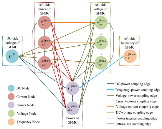
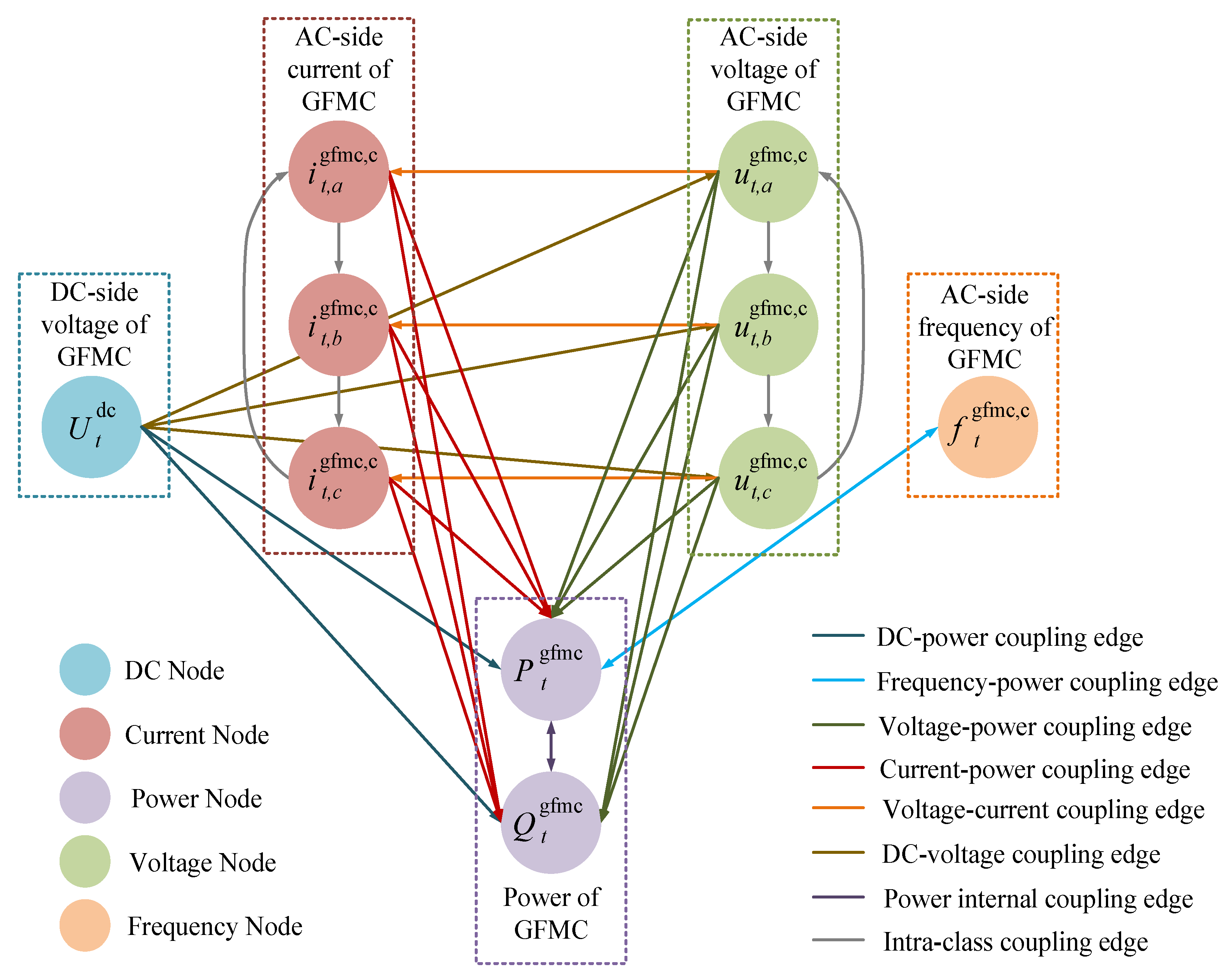
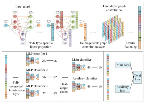
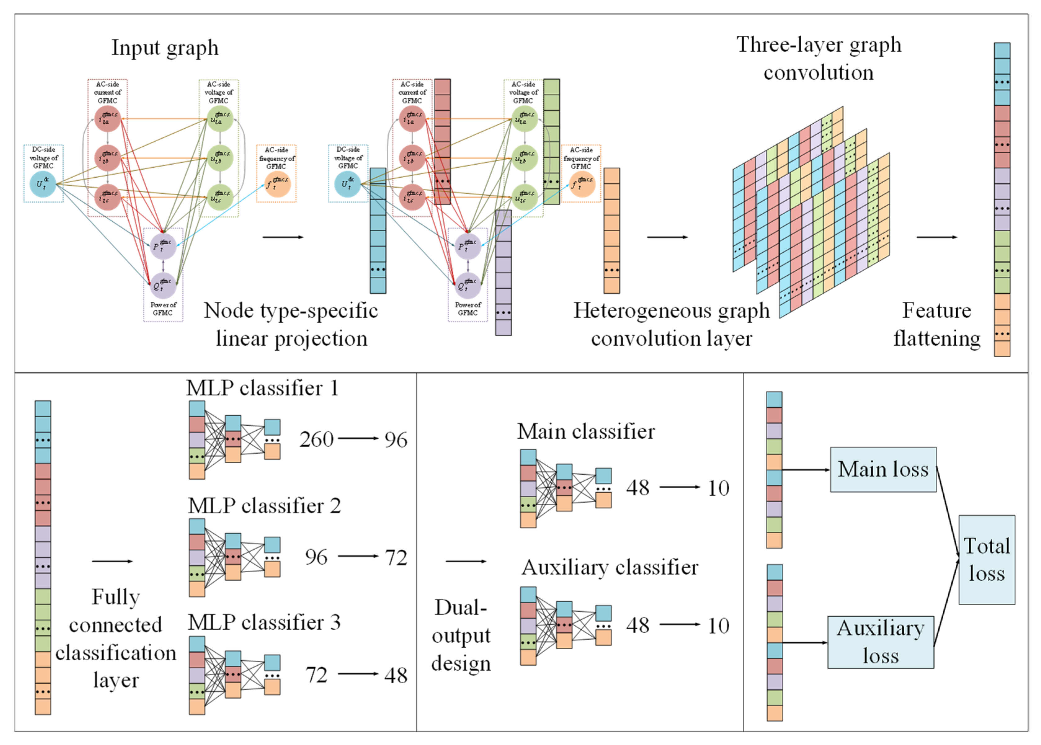
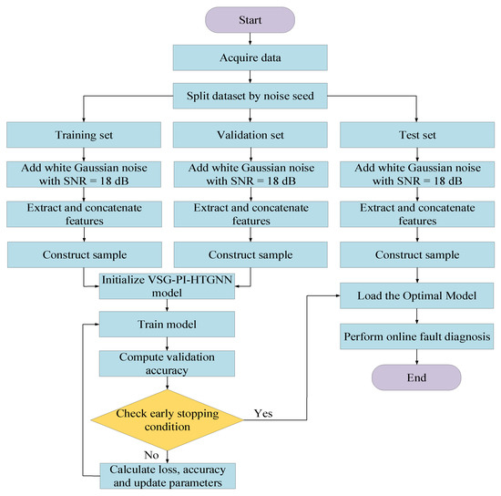
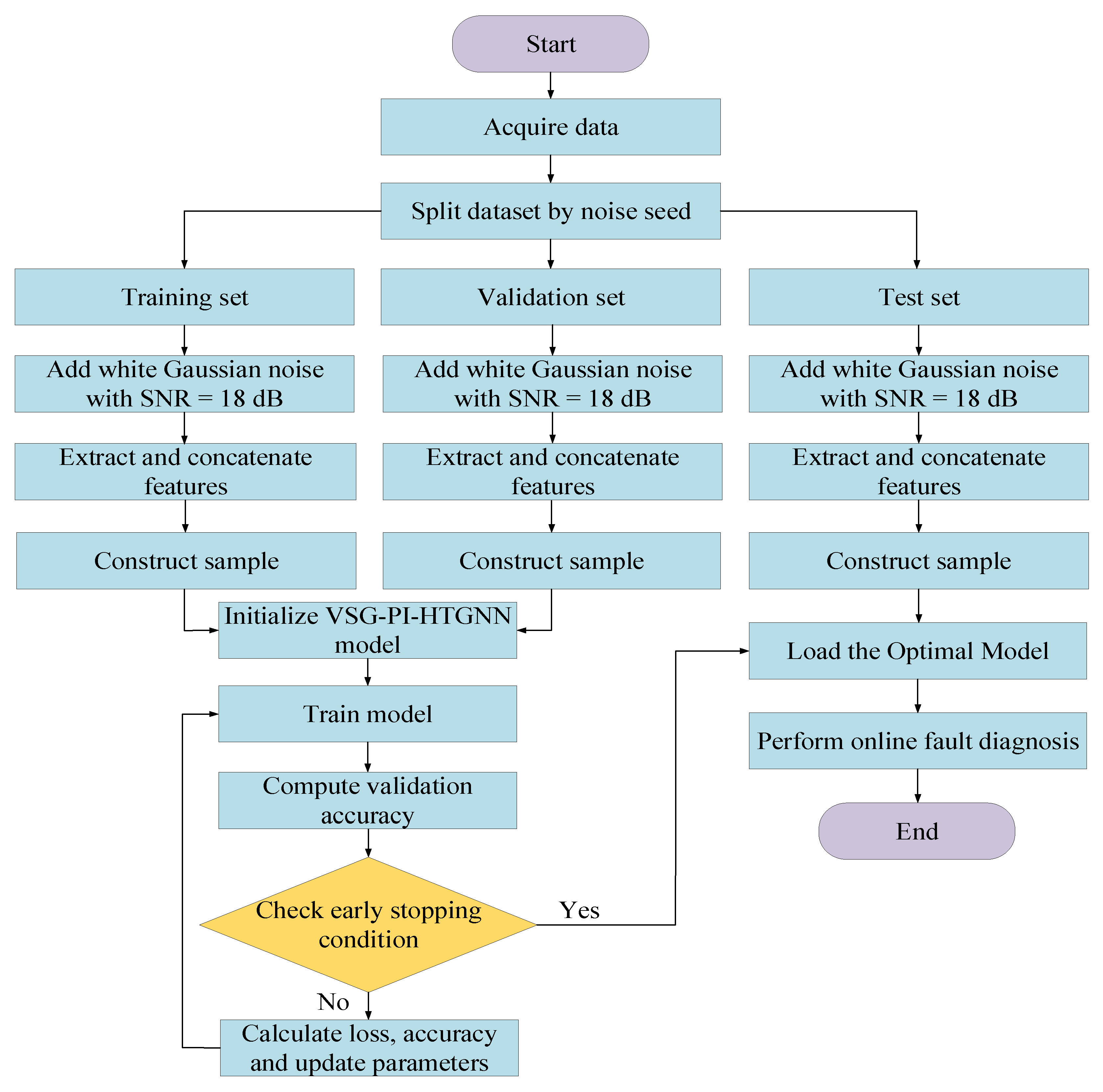
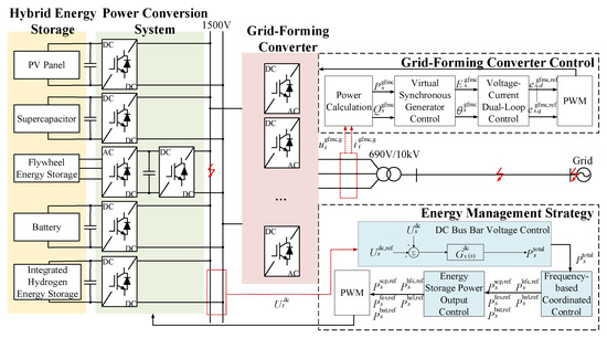
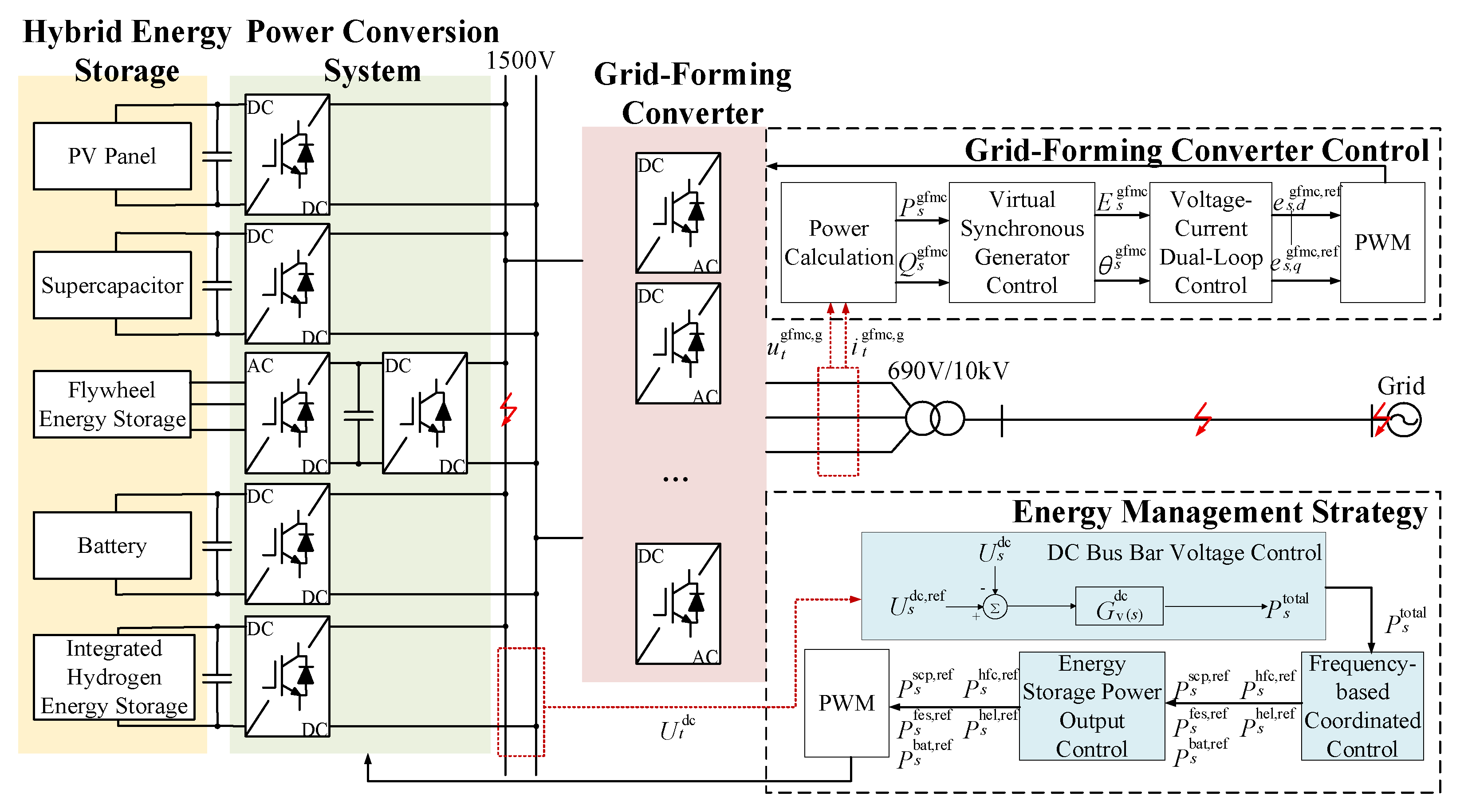
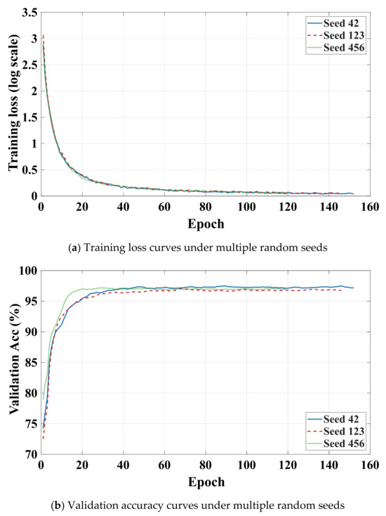
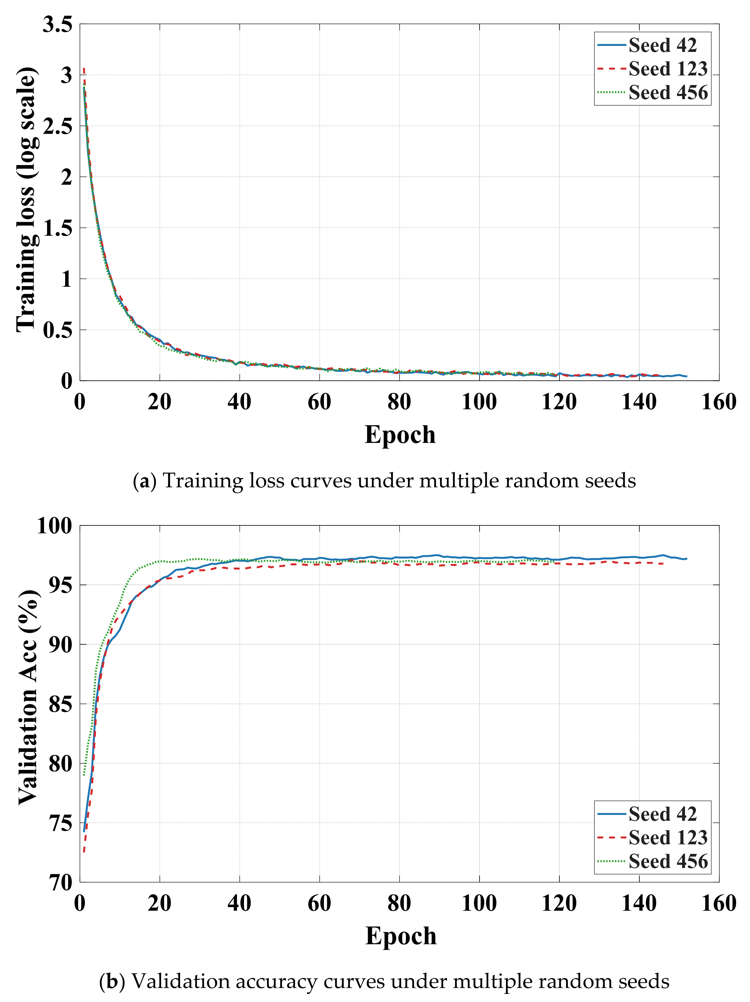
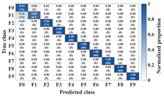
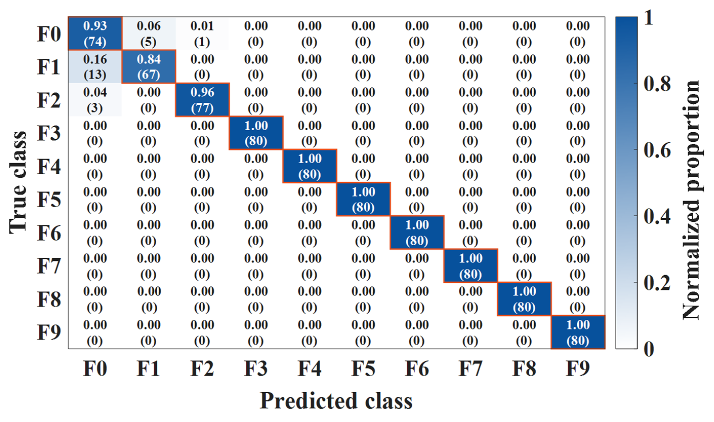
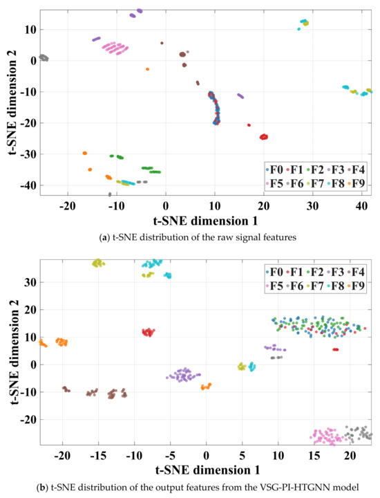
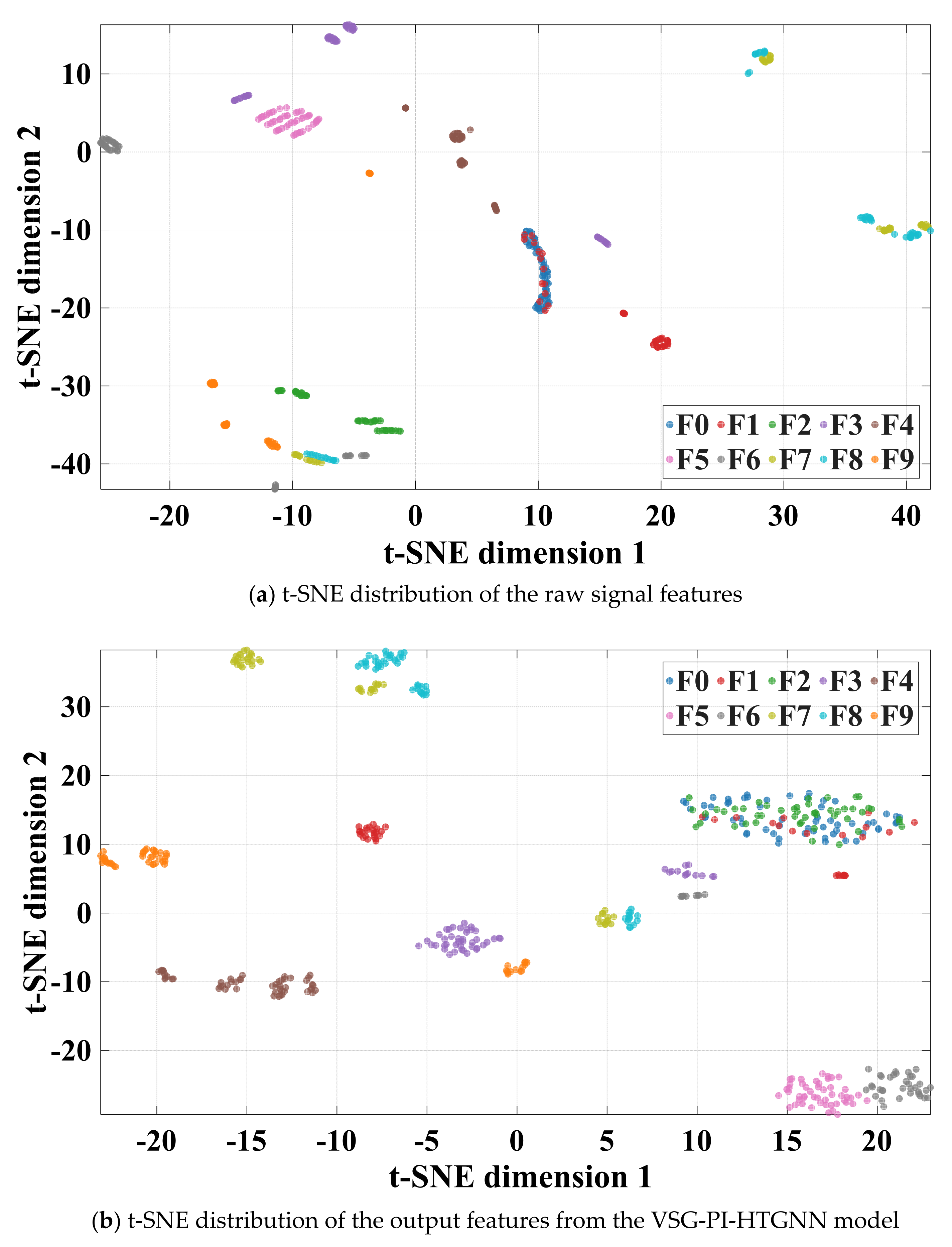
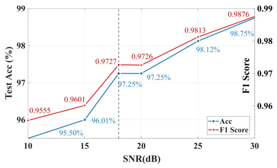
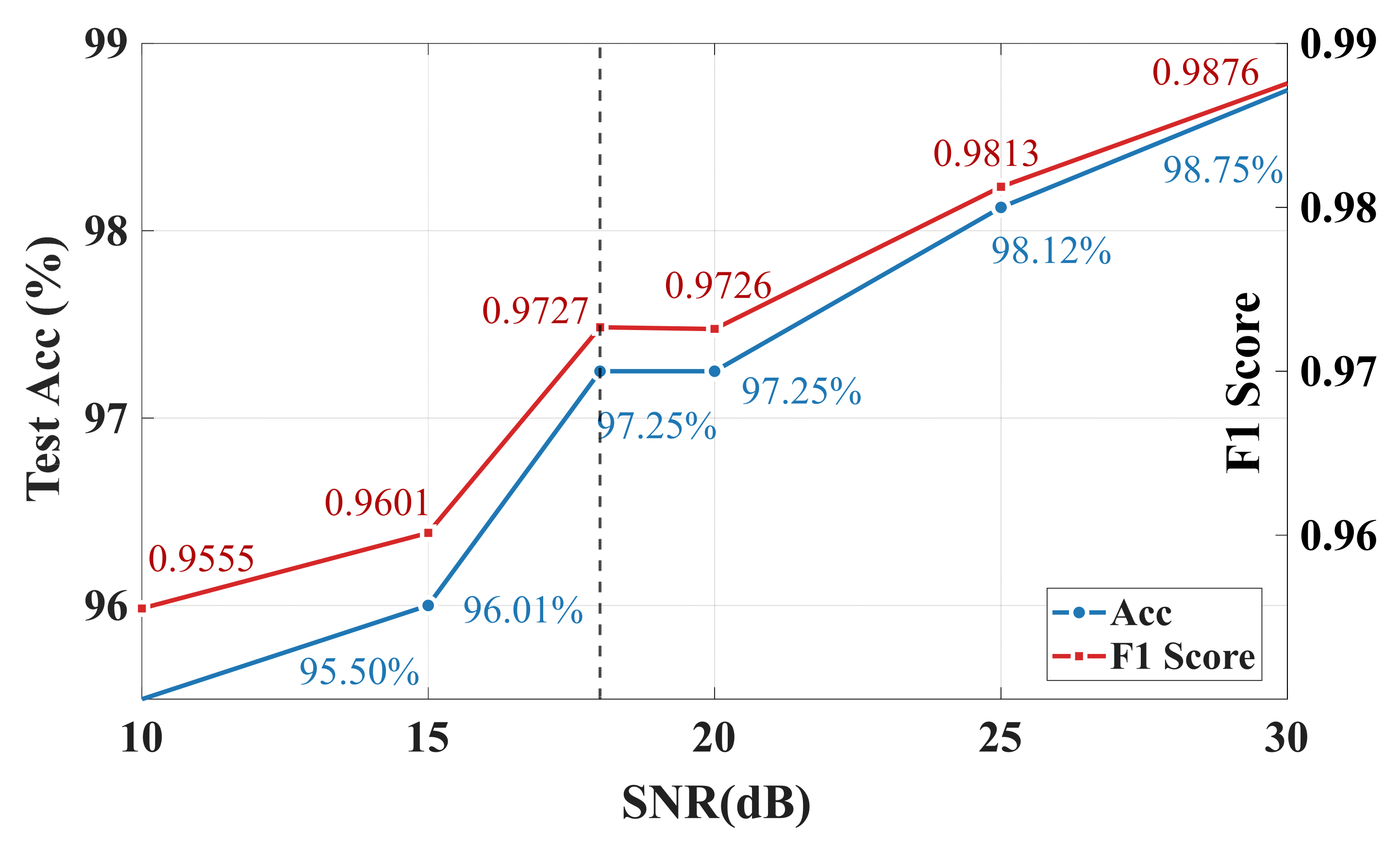
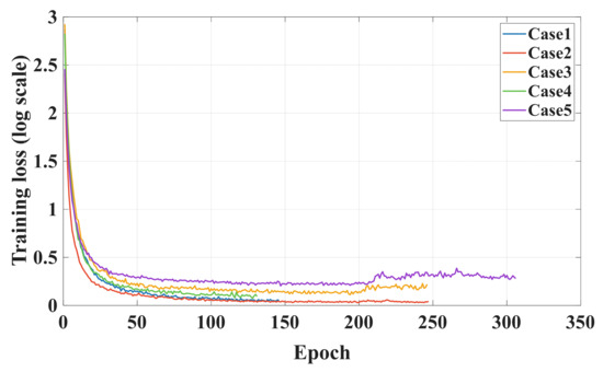
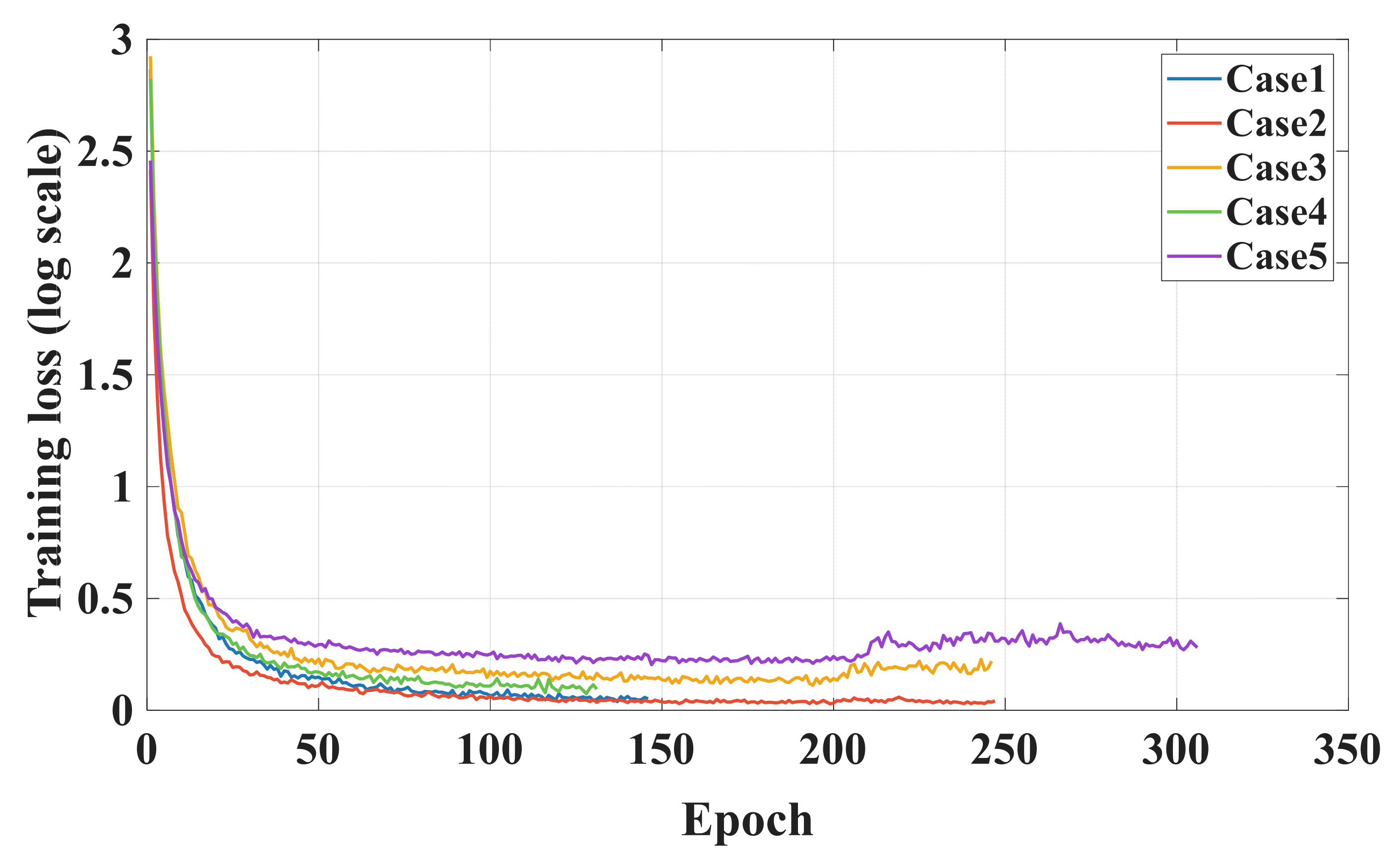
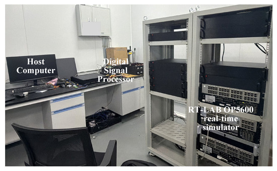
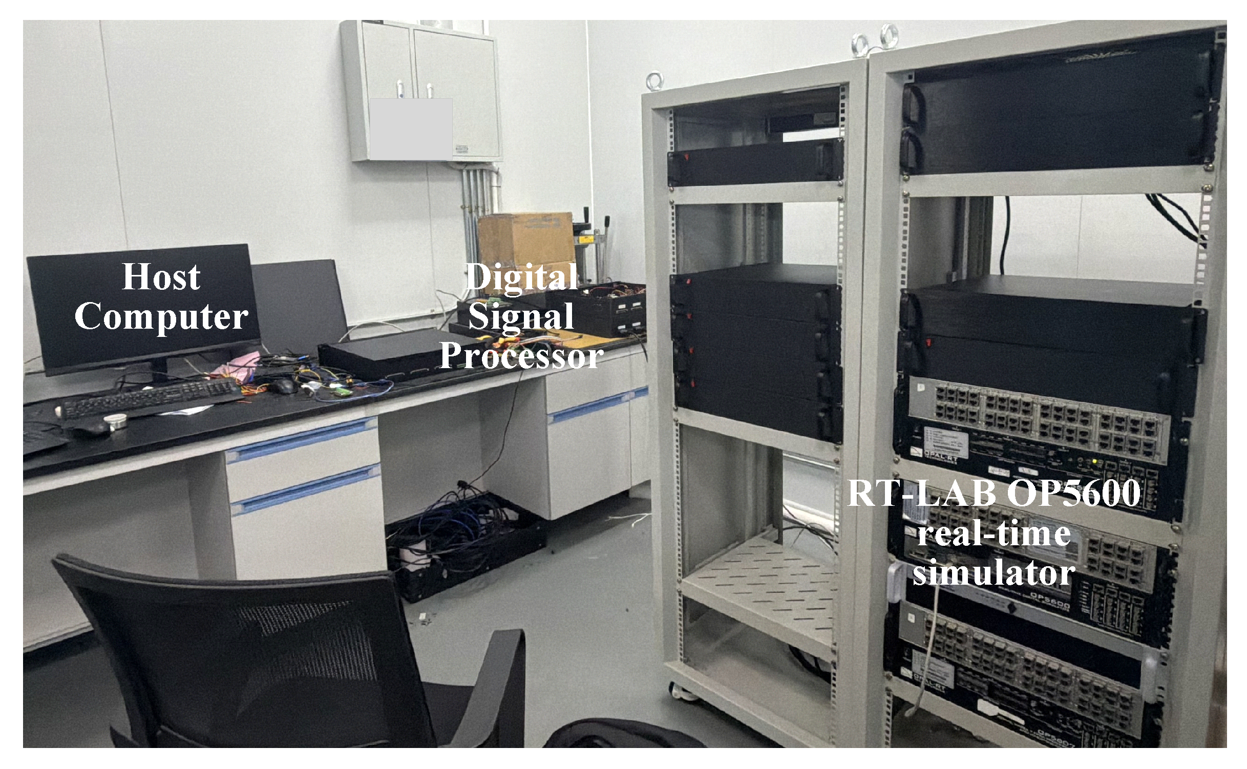
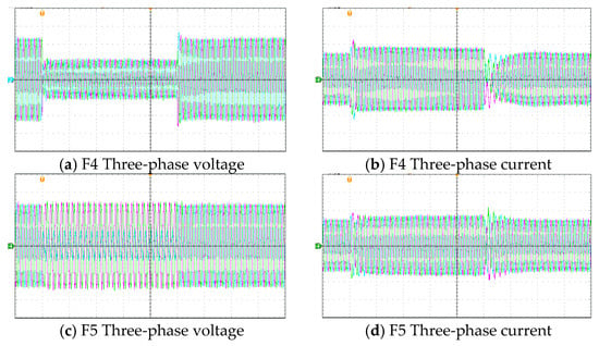
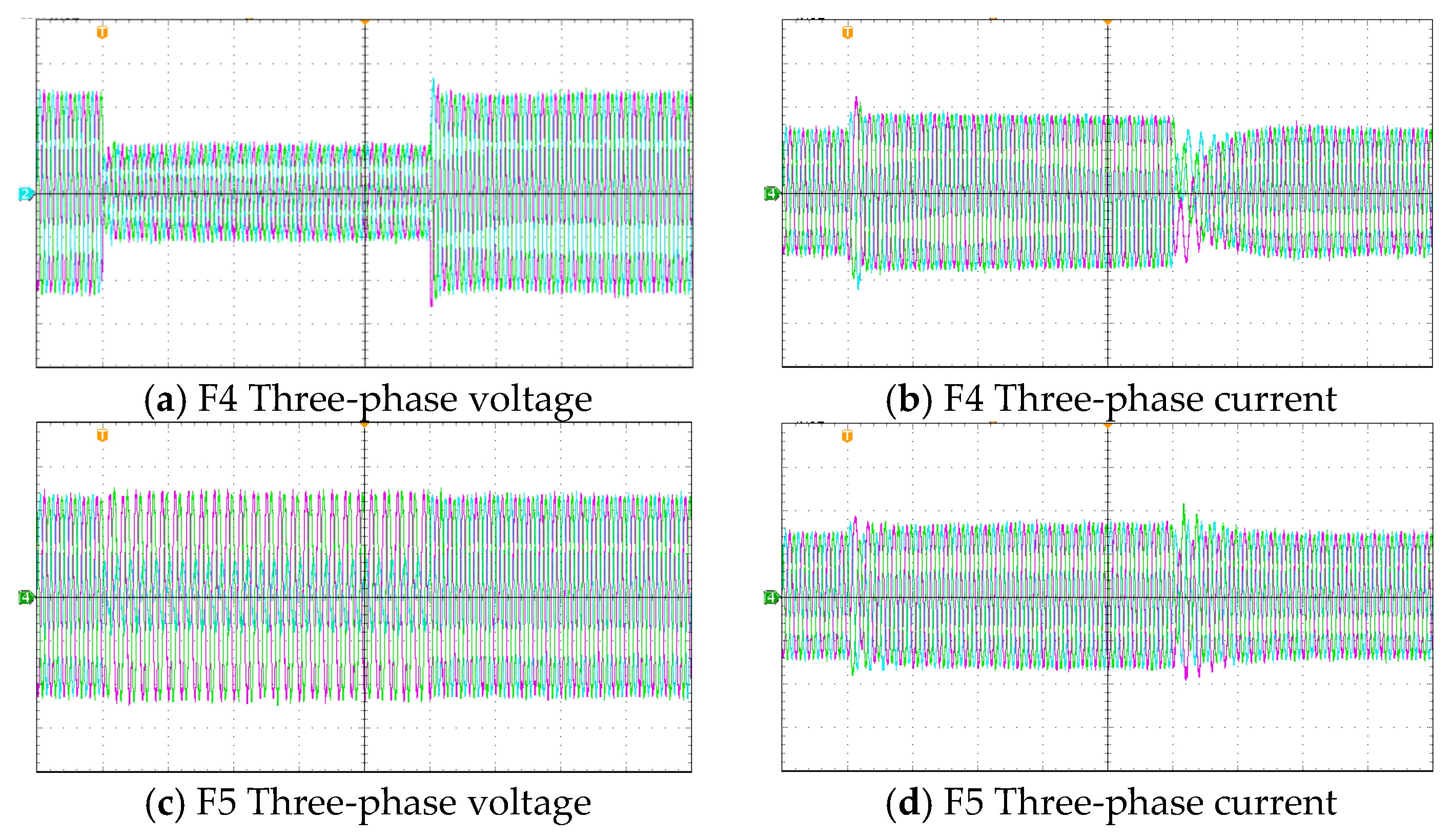

Disclaimer/Publisher’s Note: The statements, opinions and data contained in all publications are solely those of the individual author(s) and contributor(s) and not of MDPI and/or the editor(s). MDPI and/or the editor(s) disclaim responsibility for any injury to people or property resulting from any ideas, methods, instructions or products referred to in the content. |
© 2026 by the authors. Licensee MDPI, Basel, Switzerland. This article is an open access article distributed under the terms and conditions of the Creative Commons Attribution (CC BY) license.