Whole-Rock Mineral Component Identification in Shale SEM Images Using a DAM-Transformer and Analysis of NMR Response Characteristics

Abstract

Pixel-level identification of whole-rock mineral components in shale scanning electron microscopy (SEM) images is essential for characterizing shale-reservoir microstructures and quantifying mineral contents. Existing mineral identification algorithms generally cannot identify all whole-rock mineral components within a unified framework. Their overall accuracy is also limited by class imbalance, and fine-grained minerals and mineral boundaries remain difficult to segment in complex lithological backgrounds. To address these limitations, shale samples from the Lianggaoshan Formation in the Sichuan Basin were investigated, and a dynamic attention Transformer (DAM-Transformer) was developed for whole-rock mineral component identification in shale SEM images. The proposed method (1) integrates the matrix and associated minerals into a unified segmentation framework; (2) employs a hybrid loss function tailored to the feature distribution of shale SEM images to mitigate class imbalance and improve training stability and model generalizability; and (3) introduces a dynamic attention mechanism that adaptively optimizes window attention weights, focuses on mineral target regions, enhances boundary detail features, and suppresses background noise. The DAM-Transformer achieved a pixel-level mean accuracy (mAcc) of 78.12% across ten mineral classes, outperforming Mask2Former, FCN, UPerNet, DeepLabV3+, and other benchmark methods by 1.51–8.92%. Visual comparisons further demonstrated that the proposed method preserves the continuity of major mineral regions and substantially improves the identification of fine-grained minerals and complex mineral boundaries. In addition, application analysis of shale plug samples showed that the mineral contents identified by the DAM-Transformer exhibited clear response relationships with saturation–centrifugation NMR parameters, providing quantitative support for interpreting shale pore structure, fluid occurrence, and reservoir properties.

1. Introduction

The mineral composition of shale is a key indicator of reservoir lithology, pore structure, and reservoir storage capacity; consequently, its accurate identification is critical for detailed reservoir evaluation and sweet-spot selection [1]. However, clay minerals, quartz, feldspars, carbonate minerals, organic matter, and other components that coexist within shale exhibit substantial differences in particle size and commonly show indistinct local boundaries against complex matrix backgrounds [2,3,4]. Conventional manual identification and image processing methods rely heavily on expert experience, are time-consuming, and cannot consistently provide pixel-level mineral distribution information [5,6]. An intelligent segmentation method is therefore required to support the quantitative evaluation and microscale characterization of shale reservoirs.

In recent years, deep learning has been widely applied to mineral image recognition and digital rock segmentation. Li et al. [7] applied machine learning to mineral classification in SEM-EDS images, and Chen et al. [8] developed a deep learning method for mineral characterization segmentation in shale SEM images. Bihani et al. [9] developed MudrockNet for the automatic segmentation of pores and grains in mudrock SEM images. Yin et al. [10] proposed Paw-Net for fine-grained shale SEM images and subsequently introduced a semi-supervised strategy to improve performance when labeled data are limited [11]. Yasin et al. [12] applied Attention U-Net to pore structure analysis in organic-rich shale. For simultaneous multi-component identification, Li et al. [13] established a multi-component digital rock model of shale by combining CT and QEMSCAN images, Sun et al. [14] used Res-UNet for multi-mineral modeling, and Liang et al. [15] and Wang et al. [16] investigated multi-mineral segmentation in rock micro-CT images. Niu et al. [17], Karimpouli and Tahmasebi [18], Phan et al. [19], Cao et al. [20], and Alqahtani et al. [21] improved digital rock image processing workflows by reducing operator bias, applying autoencoders, performing three-dimensional segmentation, using multi-task learning, and enhancing super-resolution, respectively. For thin-section and mineral grain images, Saxena et al. [22], Filippo et al. [23], and Latif et al. [24] demonstrated the effectiveness of deep learning for mineral boundary extraction and component identification. More recently, Dong et al. [25] applied a hybrid attention mechanism to sandstone image analysis, Zheng et al. [26] used a dual-modal Vision Transformer for thin-section grain segmentation, and Koeshidayatullah et al. [27] explored attention mechanisms for quantitative petrography. Hassan et al. [28] and Knaup et al. [29] extended deep learning applications to mineral thin sections and shale microstructure identification. Recent segmentation studies have introduced more Transformer-based and foundation-model-based architectures. SegFormer combines a hierarchical Transformer encoder with a lightweight MLP decoder for efficient semantic segmentation [30], Mask2Former uses masked attention for universal image segmentation [31], and SAM provides a promptable foundation model for general image segmentation [32]. In addition, recent high-resolution Transformer architectures and large-scale visual backbones, such as HRFormer [33] and InternImage [34], have provided new strategies for preserving fine spatial details and improving dense prediction performance. For geological image analysis, Ren et al. [35] proposed a multi-channel-attention Transformer for rock thin-section image segmentation, while Fan et al. [36] developed a foundation model for rock thin-section image analysis. These studies show that image segmentation is moving toward Transformer-based representation learning and foundation models. Nevertheless, three major challenges remain. First, many methods focus on pores and matrices, specific minerals, or a limited number of components and therefore cannot simultaneously identify multiple shale minerals within a unified framework. Second, large differences in pixel abundance and particle scale cause models to favor dominant classes, limiting their mean identification performance for fine-grained minerals. Third, complex matrices, similar textures, and indistinct boundaries impair mineral region integrity and detail recognition, requiring the joint use of regional context and local boundary information.

To address the large number of mineral classes, scale variation, minority class scarcity, and boundary interference from complex shale matrices, this study proposes a dynamic attention Transformer (DAM-Transformer) for whole-rock mineral component identification in SEM images of Lianggaoshan Formation shale from the Sichuan Basin. The proposed method (1) integrates matrix and associated minerals into a unified segmentation framework; (2) uses a hybrid loss function adapted to the feature distribution of shale SEM images to mitigate class imbalance and improve training stability and model generalizability; and (3) introduces a dynamic attention mechanism that adaptively optimizes window attention weights, focuses on mineral targets, strengthens boundary detail features, and suppresses background noise. The DAM-Transformer achieved an mAcc of 78.12%, a mean intersection over union (mIoU) of 69.27%, and a mean Dice coefficient (mDice) of 84.07%, representing average improvements of 5.54, 3.64, and 3.86 percentage points, respectively, over FCN, UPerNet, DeepLabV3+, PSPNet, Mask2Former, and SegFormer. Visual comparisons showed that the DAM-Transformer preserves the continuity of major mineral regions and improves the identification of fine-grained minerals and complex boundaries. The proposed method provides technical support for mineral content quantification and shale reservoir microstructure analysis.

2. Methods

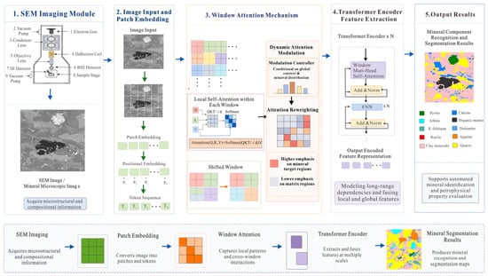
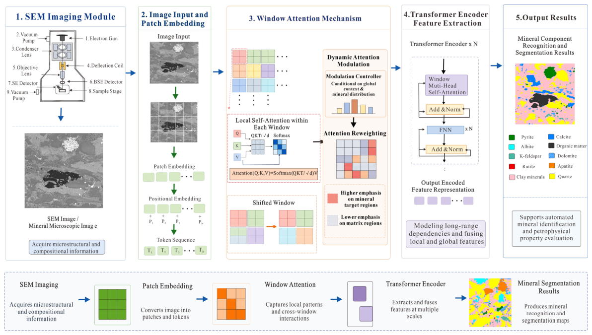
Figure 1 presents the overall architecture of the DAM-Transformer for whole-rock mineral component identification in shale SEM images. The architecture builds on the original Transformer framework [37] and shifted-window attention strategy. The architecture comprises an SEM imaging module, an image input and patch-embedding module, a window attention module, a Transformer encoder feature extraction module, and a mineral segmentation output module. The SEM imaging module acquires information on the microstructure and mineral distribution of shale samples. The image input and patch-embedding module convert continuous images into feature sequences with spatial position information. The window attention module extracts local textures, grain edges, and cross-window correlations. The Transformer encoder deeply integrates local features and establishes contextual relationships among different mineral regions. Finally, the output module generates pixel-level mineral classifications from the encoded features, enabling automatic identification and spatial localization of whole-rock mineral components.

Figure 1. Overall framework of the model.

(1)

After patch embedding and positional encoding, a shale SEM image is transformed into a structured feature sequence for whole-rock mineral identification. The input image is divided into fixed-size patches; each patch is linearly mapped to a feature vector and combined with positional encoding to retain spatial relationships among mineral grains. Unlike conventional approaches that primarily identify a single mineral or a subset of components, the DAM-Transformer incorporates pyrite, calcite, albite, organic matter, K-feldspar, dolomite, rutile, apatite, clay minerals, and quartz within a unified segmentation system. This framework simultaneously identifies matrix and associated minerals in the same image while maintaining spatial correspondence with the original image, thereby providing a more complete representation of the shale mineral composition and distribution.

(2)

The dynamic attention mechanism adaptively modifies window attention weights to improve the differential representation of complex matrix backgrounds and local mineral features. After the feature sequence enters the window attention module, correlations among patches are calculated within local windows, and shifted windows establish information exchange between adjacent regions. The dynamic attention mechanism then adjusts the attention weights according to global context and mineral distribution features. Attention is moderately dispersed over extensive matrix regions to capture more complete background information, whereas it is concentrated on mineral targets to enhance key features such as grain edges, fine-grained textures, and complex boundaries. This mechanism reduces background noise interference and improves the identification of small-scale minerals, irregular regions, and indistinct boundaries.

To clarify the difference between DAM and the standard shifted-window attention used in the Swin Transformer, standard window attention is mainly determined by the similarity among query, key, and value features, together with a relative position bias. This bias is primarily related to spatial position and cannot adaptively change according to mineral composition, matrix complexity, or boundary characteristics in different SEM images. Therefore, the DAM-Transformer introduces a dynamic modulation term generated from the input feature map into the window attention calculation:

$$DAM(Q,K,V)=Softmax\left({\displaystyle \frac{Q{K}^T}{\sqrt{d}}}+B+\alpha D(X)\right)V$$

(1)

where D(X) is the dynamic attention bias generated from the input feature map, and α is a learnable scaling factor. Compared with the standard Swin attention, DAM does not simply use shifted windows; instead, it incorporates a sample-dependent dynamic bias into the attention operation. This allows the model to adaptively adjust the attention distribution according to mineral texture, particle scale, and matrix background. The mechanism enables more dispersed attention over extensive matrix regions and more concentrated attention over fine-grained minerals and blurred boundaries, making it more suitable for shale SEM images with complex mineral assemblages, class imbalances, and indistinct mineral boundaries.

(3)

The Transformer encoder and hybrid loss function jointly improve feature integration, training stability, and generalization. The locally attended feature sequence is passed to a multi-layer Transformer encoder, in which each layer contains multi-head self-attention, a feed-forward neural network, residual connections, and normalization operations to integrate local details with global semantic information. A classification layer maps the encoded features to class probabilities for each pixel and generates the whole-rock mineral segmentation map. Because shale minerals differ substantially in abundance and particle scale, a hybrid loss function adapted to the feature distribution of shale images jointly constrains class balance, region fitting, and boundary identification during training. This design reduces the dominance of extensive clay mineral and quartz regions, improves feature learning for low-abundance minerals, and decreases feature-fitting bias.

The hybrid loss function was further formulated to provide explicit constraints on pixel-wise classification, region-level overlap, and hard-to-classify mineral pixels. It is defined as

$$L={\lambda }_{ce}{L}_{wce}+{\lambda }_{dice}{L}_{dice}+{\lambda }_{focal}{L}_{focal}$$

(2)

where L_wce, L_dice, and L_focal are the weighted cross-entropy loss, Dice loss, and focal loss, respectively, and λ_ce, λ_dice, and λ_focal are the respective weighting coefficients of the three loss terms. In this study, these coefficients were set to 0.4, 0.4, and 0.2, respectively, in order to balance pixel-level classification accuracy, mineral region integrity, and minority class recognition.

The weighted cross-entropy loss is expressed as

$$L_{wce}=-{\displaystyle \frac{1}{N}}{\displaystyle \sum _{p=1}^N{\displaystyle \sum _{c=1}^C{w}_c}}{y}_{p,c}\log ({\widehat{y}}_{p,c}+\epsilon )$$

(3)

where N is the total number of pixels, C is the number of mineral classes, y_p,c is the ground truth label of pixel p for class c, ${\widehat{y}}_{p,c}$ is the predicted probability, and ε is a small constant used to avoid numerical instability. The class weight w_c was calculated according to the inverse pixel frequency of each mineral class as follows:

$$w_c={\displaystyle \frac{C{(f_c+\epsilon )}^{-1}}{{\displaystyle \sum _{k=1}^C{(f_k+\epsilon )}^{-1}}}}$$

(4)

where f_c is the pixel frequency of the cth mineral class. This weighting strategy assigns higher weights to low-abundance minerals and reduces the dominance of extensive classes, such as clay minerals and quartz, during model training.

The Dice loss was used to constrain the spatial overlap between the predicted mineral regions and the ground truth annotations, defined as follows:

$$L_{dice}=1-{\displaystyle \frac{1}{C}}{\displaystyle \sum _{c=1}^C\frac{2{\displaystyle \sum _{p=1}^N{y}_{p,c}}{\widehat{y}}_{p,c}+\epsilon }{{\displaystyle {\displaystyle \sum _{p=1}^N}{y}_{p,c}}+{\displaystyle {\displaystyle \sum _{p=1}^N}{\widehat{y}}_{p,c}}+\epsilon }}$$

(5)

This term improves region-level consistency and helps to maintain the continuity of mineral boundaries. The focal loss is expressed as

$$L_{focal}=-{\displaystyle \frac{1}{N}}{\displaystyle \sum _{p=1}^N{\displaystyle \sum _{c=1}^C{w}_c}}{y}_{p,c}{(1-{\widehat{y}}_{p,c})}^{\gamma }\log ({\widehat{y}}_{p,c}+\epsilon )$$

(6)

where γ is the focusing parameter. In this study, γ = 2 was used to enhance the contribution of hard-to-classify pixels, including fine-grained minerals, locally mixed mineral regions, and blurred boundaries.

The sensitivity of the hybrid loss mainly depends on the relative contribution of the three loss terms. A larger weighted cross-entropy term improves minority class sensitivity but may introduce local noise along mineral boundaries. A larger Dice term enhances region-level consistency but may weaken the learning of very small mineral targets. A larger focal term increases the contribution of difficult pixels but may overemphasize uncertain boundary areas. Therefore, the adopted weighting combination provides a compromise among overall segmentation accuracy, regional consistency, and minority mineral recognition. The ablation results support this effect. Compared with the baseline Transformer, the DAM-Transformer improved the mIoU, mAcc, and mDice of all ten mineral classes, with particularly evident improvements for low-abundance or difficult-to-identify minerals such as rutile, apatite, and K-feldspar. This indicates that the hybrid loss function and dynamic attention mechanism can enhance the recognition of minority minerals and complex boundaries.

3. Research Preparation

3.1. Instrumentation and Experimental Workflow

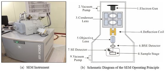
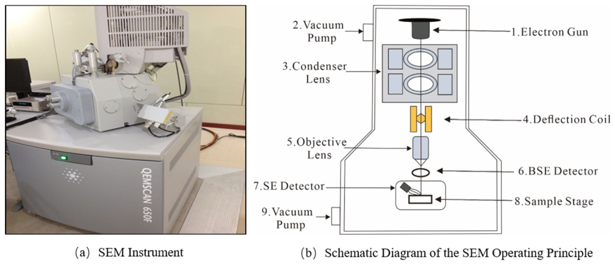
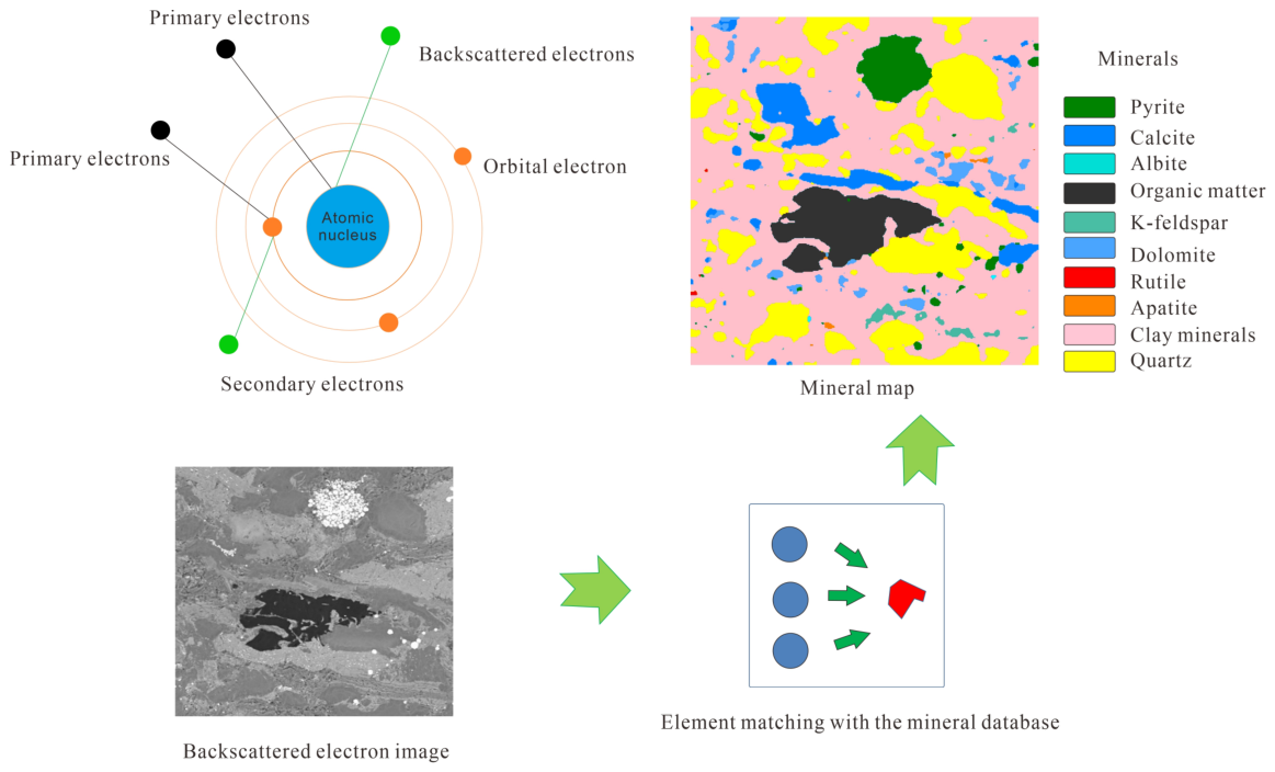
In scanning electron microscopy, signals generated by the interaction between a focused electron beam and the sample surface can be used to characterize rock microstructures and mineral components. After emission from the electron gun, the electron beam is focused by the condenser and objective lenses and scans the sample surface point by point under the control of deflection coils. Interactions between the electron beam and sample atoms generate secondary electrons, backscattered electrons, and characteristic X-rays (Figure 2). Secondary electrons primarily reveal the surface morphology, whereas the backscattered electron intensity depends on the mean atomic number of a mineral and can therefore distinguish different mineral regions. Characteristic X-rays indicate elemental composition and provide a basis for mineral identification.

Figure 2. Scanning electron microscopy (SEM): (a) SEM instrument; (b) schematic diagram of the SEM op-erating principle.

A QEMSCAN 650F (Thermo Fisher Scientific Inc., Waltham, MA, USA) automated mineral analysis system was used for microscopic scanning and mineral composition identification of the shale samples. First, backscattered electron images were acquired from the prepared samples to characterize the spatial distributions of mineral grains, pores, and fractures. Characteristic X-ray spectra were then collected at individual pixel locations to obtain the corresponding elemental combination features. Finally, the elemental compositions and backscattered electron grayscale values were matched against a mineral database to automatically classify quartz, feldspars, calcite, clay minerals, pyrite, and other components and to generate spatially resolved mineral distribution maps (Figure 3). This workflow simultaneously provides mineral type, grain morphology, and spatial distribution information for constructing the dataset used in subsequent intelligent identification.

Figure 3. Experiment workflow.

3.2. Data Sources and Preprocessing

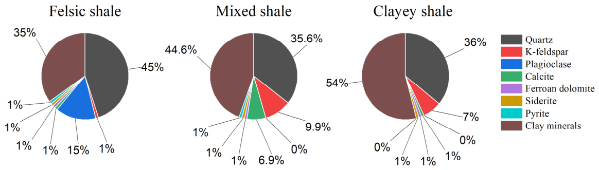
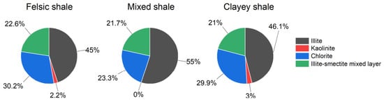
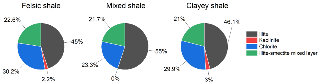
The experimental data comprised microscopic images and QEMSCAN mineral analysis results obtained from Lianggaoshan Formation shale samples in the Sichuan Basin. The samples were classified based on mineral composition as felsic, mixed, or clayey shale. Felsic shale was dominated by quartz (approximately 46%), with clay minerals and plagioclase accounting for approximately 35% and 15%, respectively. Mixed shale contained approximately 45% clay minerals, 36% quartz, 10% plagioclase, and 7% calcite. Clayey shale had the highest clay mineral content, at approximately 54% (Figure 4). The clay mineral assemblage mainly comprised illite, chlorite, and mixed-layer illite/smectite; illite accounted for approximately 46.37–55.00%, whereas the kaolinite content was low (Figure 5). These results demonstrate marked compositional differences among lithofacies and a pronounced class imbalance in the dataset.

Figure 4. Mineral composition of the whole rock of Pingye 1 well shale.

Figure 5. Mineral composition of Pingye 1 well shale clay (average content).

Representative microscopic fields of view were selected from 40 samples to construct a dataset of 740 original images and corresponding semantic labels. According to the QEMSCAN identification results, pixels were assigned to ten classes: pyrite, calcite, albite, organic matter, K-feldspar, dolomite, rutile, apatite, clay minerals, and quartz (Table 1). All images and annotation maps were resized to 384 × 384 pixels, and synchronized cropping and resizing were applied to maintain exact spatial correspondence. To avoid relying on a single random split, a five-fold repeated random validation strategy was adopted. In each run, the 740 images were divided into training and testing subsets, with 80% used for model training and 20% reserved for independent testing. Five independent partitions were generated using different random seeds. In each run, the DAM-Transformer and all benchmark models used the same training/testing split, input size, training settings, and evaluation metrics. The final results were averaged across the five runs and are reported as the mean ± standard deviation.

Table 1. QEMSCAN mineral content analysis of shale samples.

Mineral Component	Minimum Content/%	Maximum Content/%	Average Content/%
Quartz	18.69	47.40	30.27
Albite	0.00	5.88	0.90
K-feldspar	0.00	3.01	0.82
Calcite	0.06	12.11	4.38
Dolomite	0.04	5.55	1.32
Apatite	0.03	1.91	0.42
Clay minerals	46.31	77.88	59.21
Rutile	0.12	1.08	0.40
Pyrite	0.00	3.79	1.37
Organic matter	0.01	4.80	0.94

Although no external mineralogical dataset was introduced in this study, the QEMSCAN dataset was divided into independent training and testing subsets before model training. The training set was only used for parameter learning, whereas the testing set was kept completely separate and was not involved in model optimization, weight updating, or data augmentation. Therefore, the test results provide an independent internal validation of the DAM-Transformer within the available QEMSCAN dataset. This design reduces information leakage between training and testing samples and allows the segmentation performance to be evaluated on unseen SEM images from the same mineralogical dataset.

In addition, the DAM-Transformer was not trained entirely from scratch on the limited shale SEM dataset. Before being applied to the mineral identification task in this study, the Transformer-based segmentation backbone was initialized using pretrained weights from a related semantic segmentation model. This pretraining strategy provided the model with prior feature representation ability for extracting edges, textures, local structures, and region-level semantic information. The shale SEM dataset was then used for task-specific fine-tuning, allowing the model to adapt the pretrained representation to mineral grains, matrix backgrounds, and complex mineral boundaries. Therefore, although the dataset contains only 40 shale samples and 740 images, the use of pretrained Transformer segmentation features, synchronized data augmentation, and an independent training–test split helped to reduce the risk of overfitting and improved the stability of the model training.

3.3. Evaluation Metrics

The model performance was evaluated using mean accuracy (mAcc), mean intersection over union (mIoU), and mean Dice coefficient (mDice). Suppose that there are C mineral component classes in the shale core images, n_ij is the number of pixels whose ground truth class is the ith class and whose predicted class is the jth class, and n_ii is the number of pixels correctly identified as the ith mineral component by the model.

mAcc [38] is the mean classwise accuracy. It reduces the influence of extensive classes, such as quartz and clay minerals, on the overall evaluation. A higher mAcc indicates a more balanced identification across mineral classes and is calculated as follows:

$$\mathrm{mAcc}={\displaystyle \frac{1}{C}}{\displaystyle \sum _{i=1}^C\frac{n_{ii}}{{\displaystyle \sum _{j=1}^C{n}_{ij}}}}$$

(7)

where C is the total number of mineral classes, $n_{ii}$ is the number of pixels whose ground truth and predicted classes are both i, and ${\displaystyle \sum _{j=1}^C{n}_{ij}}$ is the total number of ground truth pixels belonging to class i. mAcc ranges from 0 to 1, with values closer to 1 indicating stronger mean identification performance across mineral classes.

mIoU [39] is the mean intersection-over-union value between the predicted and ground truth regions of each class. It accounts for both false negatives and false positives and therefore evaluates mineral region extent and boundaries. A higher mIoU indicates greater overlap between predicted and ground truth regions and is calculated as follows:

$$\mathrm{mIoU}={\displaystyle \frac{1}{C}}{\displaystyle \sum _{i=1}^C\frac{n_{ii}}{{\displaystyle {\displaystyle \sum _{j=1}^C}{n}_{ij}}+{\displaystyle {\displaystyle \sum _{j=1}^C}{n}_{ji}}-n_{ii}}}$$

(8)

where $n_{ii}$ is the number of pixels in the intersection between the predicted region and the ground truth region for the ith mineral component, ${\displaystyle \sum _{j=1}^C{n}_{ij}}$ represents the total number of pixels whose ground truth category belongs to the ith mineral component, and ${\displaystyle \sum _{j=1}^C{n}_{ji}}$ represents the total number of pixels predicted as the ith mineral component by the model. ${\displaystyle {\displaystyle \sum _{j=1}^C}{n}_{ij}}+{\displaystyle {\displaystyle \sum _{j=1}^C}{n}_{ji}}-n_{ii}$ is the number of pixels in the union between the predicted region and the ground truth region. The mIoU value ranges from 0 to 1. A larger mIoU indicates a higher degree of overlap between the predicted results and the ground truth annotations, suggesting better mineral component segmentation performance.

mDice [40] is the mean Dice coefficient between the predicted and ground truth regions of each class. Because it is sensitive to changes in regional overlap, it provides a complementary evaluation of small-scale minerals and complex boundaries. A higher mDice indicates greater agreement between the prediction and annotation and is calculated as follows:

$$\mathrm{mDice}={\displaystyle \frac{1}{C}}{\displaystyle \sum _{i=1}^C\frac{2n_{ii}}{{\displaystyle {\displaystyle \sum _{j=1}^C}{n}_{ij}}+{\displaystyle {\displaystyle \sum _{j=1}^C}{n}_{ji}}}}$$

(9)

where $n_{ii}$ is the number of pixels in the intersection between the predicted region and the ground truth region for the ith mineral component, ${\displaystyle \sum _{j=1}^C{n}_{ij}}$ represents the total number of pixels whose ground truth category belongs to the ith mineral component, and ${\displaystyle \sum _{j=1}^C{n}_{ji}}$ represents the total number of pixels predicted as the ith mineral component by the model. The mDice value ranges from 0 to 1. A value closer to 1 indicates a higher consistency between the predicted region and the ground truth annotation, suggesting more accurate mineral component segmentation.

3.4. Training Environment and Parameter Settings

The hardware and software configurations used to train and test the DAM-Transformer are summarized in Table 2, including the deep learning framework, programming language, operating system, GPU, CPU, and memory capacity.

Table 2. Network model training environment.

Training Environment	Training Environment Configuration
Operating System	Windows 11
GPU	NVIDIA GeForce RTX 3090
CPU	Core i9-12900K
Memory	64 GB
Programming Language	Python3.10
Deep Learning Framework	PyTorch 2.4.0
CUDA	11.8
Integrated Development Environment	PyCharm 2023.1

To improve reproducibility, the detailed network and training settings are provided here. The input image size was set to 384 × 384 pixels, the patch size was set to 4 × 4, and the initial embedding dimension was set to 96. The Transformer encoder contained four stages, with encoder depths of [2, 2, 6, 2] and attention heads of [3, 6, 12, 24]. The window size was set to 8 × 8. Shifted-window attention was implemented by shifting the window by half the window size in alternating blocks, enabling information exchange between neighboring windows while maintaining computational efficiency. The MLP expansion ratio was set to 4, and dropout was used to reduce overfitting.

The model was trained using the AdamW optimizer. The initial learning rate was set to 1.0 × 10⁻⁴. The batch size was set to 8, the maximum number of epochs was 150, and the weight decay was set to 1.0 × 10⁻⁴. To increase data diversity and reduce overfitting, synchronized data augmentation was applied to images and labels. All models were trained and tested under the same settings to ensure a fair comparison.

4. Results and Discussion

To systematically evaluate the effectiveness of the DAM-Transformer, it was compared with Mask2Former [31], Transformer [41], FCN [42], UperNet [43], DeepLabV3+ [44], PSPNet [45], and SegFormer [30] using identical data splits, input dimensions, and training environments. In addition, an ablation study comparing the DAM-Transformer with the baseline Transformer was conducted to evaluate the contributions of the dynamic attention mechanism and hybrid loss function to mineral identification performance. The experiments assessed training convergence, overall evaluation metrics, ablation study results, and visual mineral segmentation performance.

4.1. Comparison of Training Processes

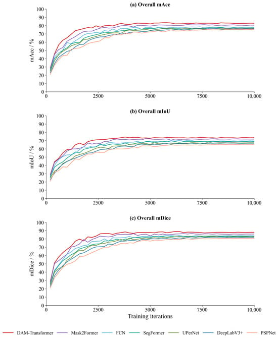
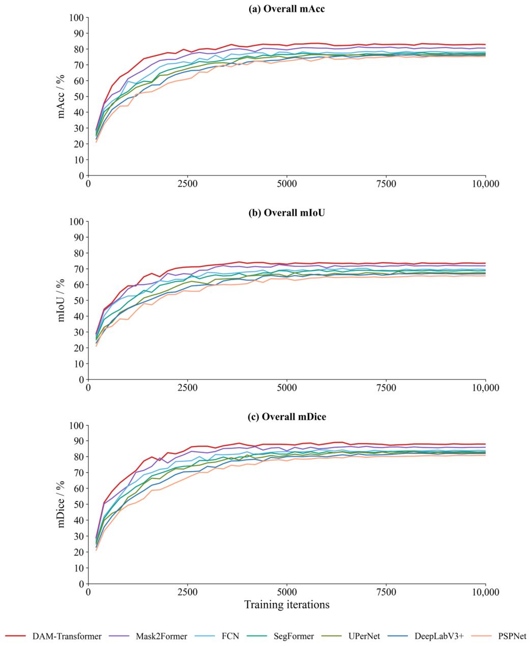
Figure 6 presents the validation-set mAcc, mIoU, and mDice curves of the evaluated algorithms during training. Overall, all models showed rapid increases in the three metrics in the early training stage, indicating that they can quickly learn the basic differences between mineral grains and the matrix background within a limited number of iterations. As the number of training iterations increased, the curves gradually became stable, suggesting that the model performances have generally converged. Among all evaluated methods, DAM-Transformer showed the fastest improvement and the highest convergence level for all three metrics. In particular, after approximately 3000 iterations, its performance advantage became stable, and it consistently maintained the best performance during the subsequent training stage. In contrast, Mask2Former, FCN, SegFormer, UPerNet, DeepLabV3+, and PSPNet also gradually converged, but their final convergence levels were lower than that of DAM-Transformer, and some models still exhibited slight fluctuations in the middle and late training stages.

Figure 6. Comparison of overall algorithm evaluation metrics during training.

Regarding individual metrics, DAM-Transformer obtained the highest mAcc, indicating strong recognition of both dominant and low-abundance mineral components. Its mIoU remained the highest and most stable in the middle and late training stages, suggesting better preservation of mineral region extent and boundary continuity. The mDice curve further confirmed stronger agreement between predicted regions and ground truth annotations. Overall, the dynamic attention mechanism enhances the model’s focus on key mineral regions and complex boundaries, while the hybrid loss function reduces the effect of class imbalance, thereby improving training stability and mineral identification accuracy.

4.2. Comparison of Evaluation Metrics

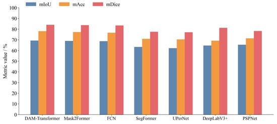
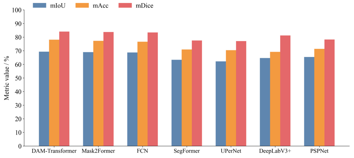
Figure 7 and Table 3 summarize the overall evaluation results of the seven models. To strengthen the statistical reliability of the comparison, each model was evaluated through repeated runs, and the results are reported as the mean ± standard deviation in Table 3. The small standard deviations indicate that the model performance only fluctuated slightly across repeated evaluations, supporting the stability and reliability of the observed results under the same experimental settings. DAM-Transformer achieved the best overall performance across all evaluation metrics, with an mAcc of 78.13%, mIoU of 69.29%, and mDice of 84.27%. Compared with Mask2Former, FCN, UPerNet, DeepLabV3+, PSPNet, and SegFormer, DAM-Transformer improved mAcc by 1.12, 1.44, 7.71, 9.03, 6.77, and 7.23 percentage points, respectively. The corresponding improvements in mIoU were 0.15, 0.47, 6.92, 4.62, 3.87, and 5.95 percentage points, while the mDice improvements were 0.58, 1.15, 7.00, 2.97, 5.92, and 6.74 percentage points, respectively.

Figure 7. Comparison of overall evaluation metrics of different models.

Table 3. Comparison of overall evaluation metrics of different models.

Model	mAcc/%	mIoU/%	mDice/%
DAM-Transformer	78.12 ± 0.0020	69.27 ± 0.0321	84.07 ± 0.0225
Mask2Former	77.01 ± 0.0202	69.14 ± 0.0213	83.69 ± 0.0240
FCN	76.69 ± 0.0110	68.82 ± 0.0402	83.12 ± 0.0215
UPerNet	70.42 ± 0.0122	62.37 ± 0.0431	77.27 ± 0.0312
DeepLabV3+	69.10 ± 0.0420	64.67 ± 0.0150	81.30 ± 0.0220
PSPNet	71.36 ± 0.0214	65.42 ± 0.0181	78.35 ± 0.0240
SegFormer	70.90 ± 0.0312	63.34 ± 0.0012	77.53 ± 0.0104

Note: The underlined model represents the proposed DAM-Transformer model developed in this study.

Among the benchmark models, Mask2Former and FCN achieved the most competitive overall performance, especially in terms of mIoU and mDice, indicating that mask-query-based attention segmentation and convolutional feature extraction can effectively capture mineral region information in shale SEM images. DeepLabV3+ also showed a relatively strong mDice value, suggesting that its multi-scale contextual modeling contributes to improved consistency in mineral region segmentation. Nevertheless, DAM-Transformer consistently achieved the highest values for mAcc, mIoU, and mDice. Relative to the average results of the six benchmark methods, DAM-Transformer improved mAcc, mIoU, and mDice by 5.54, 3.64, and 3.86 percentage points, respectively. These results demonstrate that the proposed DAM-Transformer improves class-balanced identification, mineral region overlap accuracy, and prediction region consistency, showing better adaptability to fine-grained minerals, complex boundaries, and class imbalance in shale SEM images.

Under a unified input size, the computational complexity and inference efficiency of different models were compared (Table 4). PSPNet, SegFormer, FCN, UPerNet, and DeepLabV3+ showed high inference throughput, with FPS values of 78.80–91.46 img/s and per-image inference times of 10.9–13.5 ms. DAM-Transformer had 250.97 M parameters, a peak GPU memory usage of 1124.69 MB, an inference time of 51.599 ms, and FPS value of 19.38, reflecting the computational cost introduced by dynamic attention and complex feature interaction. The computational cost of DAM-Transformer is well matched with its performance improvement. It achieved the highest mAcc, mIoU, and mDice values of 78.12%, 69.27%, and 84.07%, respectively, outperforming the average of the six benchmark models by 5.54, 3.64, and 3.86 percentage points. In particular, the improvement in mIoU indicates better preservation of mineral region integrity and boundary consistency, as well as stronger recognition of fine-grained minerals under class-imbalanced conditions. From an application perspective, the inference time of DAM-Transformer was only 51.599 ms per SEM image, which is far shorter than the several hours typically required for QEMSCAN, NMR, or conventional petrophysical experiments. Therefore, DAM-Transformer provides high mineral identification accuracy and stable segmentation performance while maintaining practical application efficiency, making it suitable for shale reservoir micro-characterization and quantitative whole-rock mineral identification.

Table 4. Computational complexity and inference efficiency of different benchmark models.

Model	Params/M	FLOPs/G	Inference Time/ms	FPS/Img s−1	Peak GPU Memory/MB
DAM-Transformer	250.97	35.07	51.599	19.38	1124.69
Mask2Former	215.45	35.07	53.166	18.81	988.03
FCN	49.49	57.07	11.490	87.03	311.47
UperNet	66.41	12.86	11.720	85.32	312.81
DeepLabV3+	43.58	57.07	12.691	78.80	288.47
PSPNet	48.97	57.07	10.933	91.46	308.25
SegFormer	52.45	55.49	13.523	89.23	398.21

4.3. Ablation Study

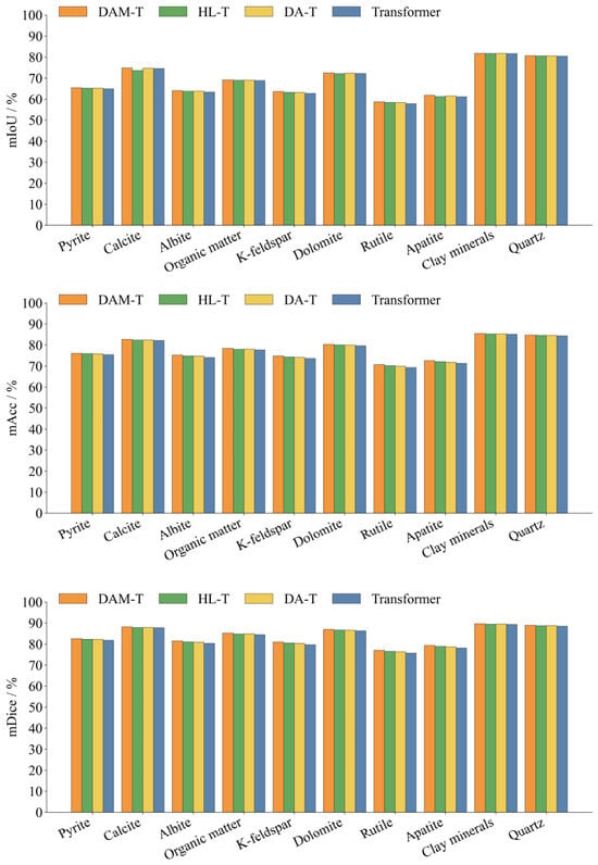
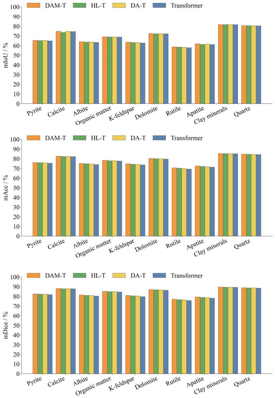
To evaluate the individual and combined contributions of the dynamic attention mechanism and hybrid loss function, an ablation study was conducted using four model variants: the baseline Transformer, Transformer with the dynamic-attention mechanism (DA-T), Transformer trained with the hybrid loss function (HL-T), and complete model integrating both modules (DAM-T) (Table 5; Figure 8). The ablation results are reported as the mean ± standard deviation, which indicate the stability of repeated evaluations for each model variant. Across the ten mineral classes, the standard deviations of mIoU, mAcc, and mDice remained small for DAM-T, HL-T, DA-T, and the baseline Transformer, suggesting that the performance differences among the ablation variants were stable rather than being caused by random fluctuations. Compared with the baseline Transformer, DA-T improved the average mIoU, mAcc, and mDice by 0.26, 0.41, and 0.41 percentage points, respectively, indicating that dynamic attention enhances the representation of local mineral textures, fine-grained targets, and irregular boundaries. The improvements of DA-T were particularly evident for rutile, albite, and K-feldspar, whose mIoU values increased by 0.48, 0.45, and 0.41 percentage points, respectively.

Table 5. Ablation study results.

Mineral Components	mIoU/%				mAcc/%				mDice/%
	DAM-T	HL-T	DA-T	Transformer	DAM-T	HL-T	DA-T	Transformer	DAM-T	HL-T	DA-T	Transformer
Pyrite	65.39 ± 0.521	65.24 ± 0.520	65.18 ± 0.526	64.97 ± 0.521	76.10 ± 0.512	75.95 ± 0.510	75.82 ± 0.515	75.40 ± 0.531	82.60 ± 0.523	82.33 ± 0.512	82.25 ± 0.410	81.84 ± 0.423
Calcite	74.75 ± 0.510	73.16 ± 0.423	74.23 ± 0.415	74.57 ± 0.422	82.70 ± 0.442	82.38 ± 0.421	82.45 ± 0.421	82.20 ± 0.340	88.20 ± 0.421	87.92 ± 0.410	87.98 ± 0.511	87.74 ± 0.526
Albite	64.12 ± 0.512	63.75 ± 0.512	63.82 ± 0.511	63.37 ± 0.342	75.20 ± 0.540	74.83 ± 0.524	74.68 ± 0.326	74.10 ± 0.442	81.50 ± 0.642	81.04 ± 0.511	80.88 ± 0.321	80.34 ± 0.431
Organic matter	69.20 ± 0.421	68.69 ± 0.515	69.05 ± 0.614	68.81 ± 0.430	78.20 ± 0.629	78.02 ± 0.414	78.10 ± 0.431	77.70 ± 0.623	85.20 ± 0.323	84.86 ± 0.623	84.92 ± 0.524	84.54 ± 0.330
K-feldspar	63.12 ± 0.520	63.25 ± 0.512	63.11 ± 0.513	62.77 ± 0.521	74.80 ± 0.337	74.35 ± 0.331	74.18 ± 0.542	73.60 ± 0.421	81.00 ± 0.412	80.55 ± 0.321	80.35 ± 0.622	79.74 ± 0.421
Dolomite	72.50 ± 0.412	72.10 ± 0.513	72.35 ± 0.415	72.17 ± 0.622	80.14 ± 0.421	80.05 ± 0.416	79.98 ± 0.429	79.70 ± 0.226	87.00 ± 0.615	86.72 ± 0.430	86.65 ± 0.312	86.34 ± 0.525
Rutile	58.34 ± 0.514	58.40 ± 0.412	58.30 ± 0.311	57.80 ± 0.323	70.70 ± 0.520	70.20 ± 0.512	69.95 ± 0.512	69.30 ± 0.329	77.10 ± 0.321	76.58 ± 0.532	76.35 ± 0.415	75.74 ± 0.626
Apatite	61.87 ± 0.511	61.25 ± 0.311	61.52 ± 0.312	61.17 ± 0.420	72.60 ± 0.634	72.10 ± 0.441	71.85 ± 0.314	71.30 ± 0.531	79.40 ± 0.425	78.95 ± 0.425	78.70 ± 0.516	78.14 ± 0.421
Clay minerals	81.52 ± 0.312	81.72 ± 0.512	81.75 ± 0.413	81.62 ± 0.310	85.50 ± 0.436	85.32 ± 0.446	85.36 ± 0.412	85.20 ± 0.330	89.70 ± 0.521	89.48 ± 0.521	89.55 ± 0.519	89.34 ± 0.323
Quartz	80.70 ± 0.421	80.48 ± 0.615	80.65 ± 0.510	80.47 ± 0.413	84.80 ± 0.541	84.62 ± 0.537	84.65 ± 0.521	84.40 ± 0.532	89.00 ± 0.620	88.75 ± 0.620	88.80 ± 0.612	88.54 ± 0.412

Figure 8. Comparison of evaluation metrics for Transformer, DA-T, HL-T, and DAM-Transformer.

HL-T mainly improved class-balanced recognition and regional consistency. Compared with the baseline Transformer, HL-T increased the average mAcc and mDice by 0.49 percentage points, indicating that the hybrid loss function reduces the dominance of high-abundance minerals and improves the recognition stability of low-abundance components. Its improvement in mIoU was relatively limited, suggesting that this module mainly strengthens class-level learning.

The complete DAM-T achieved the best overall performance, improving the average mIoU, mAcc, and mDice by 0.48, 0.83, and 0.84 percentage points over the baseline Transformer, respectively. DAM-T obtained high mIoU values for clay minerals, quartz, and calcite, and also improved the recognition of low-abundance minerals such as rutile, apatite, and K-feldspar. These results demonstrate that dynamic attention and hybrid loss play complementary roles in improving mineral feature representation and class-balanced segmentation.

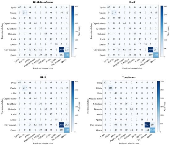
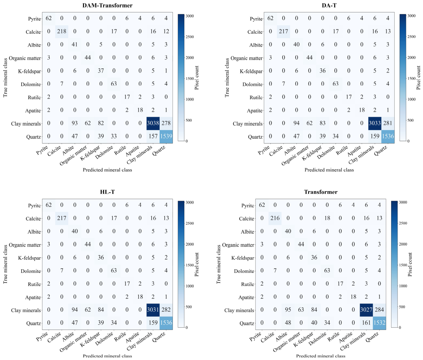
The confusion matrices of the four models are dominated by diagonal elements, indicating that most mineral pixels were correctly classified (Figure 9). Compared with the baseline Transformer, DA-T, HL-T, and DAM-Transformer all improved the recognition of major mineral classes, with the complete DAM-Transformer showing the most evident improvement. Specifically, DAM-Transformer increased the correctly classified pixels of clay minerals, quartz, and calcite to 3038, 1539, and 218, respectively, and also improved the identification of albite and K-feldspar. Misclassifications mainly occurred among clay minerals, quartz, albite, and K-feldspar, while some calcite pixels were misclassified as dolomite. These errors are related to similar SEM grayscale and texture features, as well as the intergrowth of fine-grained minerals with the matrix. Overall, dynamic attention helps reduce confusion in complex boundaries and fine-grained targets, while the hybrid loss function alleviates class imbalance bias. Their combination further improves the stability of mineral segmentation in complex shale SEM images.

Figure 9. Comparison of confusion matrices for Transformer, DA-T, HL-T, and DAM-Transformer.

To further evaluate the statistical significance of the performance improvement introduced by the DAM-Transformer, paired statistical analysis was conducted using the results from five repeated runs. The original Transformer was used as the baseline model, and each run of the DAM-Transformer was paired with the corresponding run of the Transformer under the same experimental setting. For each evaluation metric, the paired difference was calculated as follows:

$${\mathrm{d}}_{\mathrm{i}}=\mathrm{X}\{\mathrm{DAM},\mathrm{i}\}-\mathrm{X}\{\mathrm{Transformer},\mathrm{i}\}$$

(10)

where X{DAM,i and X{Transformer,i} are the metric values for DAM-Transformer and the original Transformer in the ith repeated run, respectively. The mean and standard deviation of the paired differences were calculated as follows:

$$\overline{d}={\displaystyle \frac{1}{n}}{\displaystyle \sum _{i=1}^n{d}_i}$$

(11)

$$s_d=\sqrt{{\displaystyle \frac{{\displaystyle \sum _{i=1}^n{(d_i-\overline{d})}^2}}{n-1}}}$$

(12)

where $\bar{d}$ is the mean paired difference, $s_d$ is the standard deviation of the paired differences, and n is the number of repeated runs. In this study, $n=5$. The paired t-test statistic was calculated as follows:

$$t={\displaystyle \frac{\overline{d}}{s_d/\sqrt{n}}}$$

(13)

where $t$ is the paired t-test statistic. The two-tailed p value was calculated as follows:

$$p=2\left[1-F_t\left(\left|t\right|,n-1\right)\right]$$

(14)

where $p$ is the two-tailed significance probability and $F_t$ is the cumulative distribution function of the t distribution with n − 1 degrees of freedom. In addition, Cohen’s d was calculated to quantify the effect size, defined as

$$d={\displaystyle \frac{\overline{d}}{s_d}}$$

(15)

where $d$ is Cohen’s d for paired samples. A larger absolute value of $d$ indicates a stronger effect size.

As shown in Table 6, the DAM-Transformer achieved higher mean values than the original Transformer for all three evaluation metrics. The mean improvements were 4.57 ± 0.48 percentage points for mIoU, 8.82 ± 0.69 percentage points for mAcc, and 5.97 ± 2.06 percentage points for mDice. The corresponding p values were 0.000029, 0.000009, and 0.002906, respectively, all of which are lower than 0.05. These results indicate that the improvements of the DAM-Transformer over the original Transformer were statistically significant. In addition, the Cohen’s d values were 9.527, 12.737, and 2.902 for mIoU, mAcc, and mDice, respectively, indicating large effect sizes. Therefore, the proposed DAM-Transformer not only improved the numerical performance but also produced statistically significant and substantial practical gains over the baseline Transformer.

Table 6. Paired t-test and Cohen’s d results comparing Transformer and DAM-Transformer.

Metric	Transformer Raw Data/%	Transformer Mean ± SD/%	DAM-Transformer Raw Data/%	DAM-Transformer Mean ± SD/%	p Value	Cohen’s d
mIoU	65.12, 64.79, 64.33, 65.14, 64.12	64.70 ± 0.46	69.23, 69.2485, 69.27, 69.2915, 69.31	69.27 ± 0.03	0.000029	9.527
mAcc	70.12, 69.79, 68.33, 69.14, 69.12	69.30 ± 0.69	78.1175, 78.1187, 78.1200, 78.1213, 78.1225	78.12 ± 0.002	0.000009	12.737
mDice	78.12, 74.79, 80.33, 79.14, 78.12	78.10 ± 2.06	84.04, 84.0594, 84.07, 84.08, 84.10	84.07 ± 0.02	0.002906	2.902

4.4. Visual Comparison of Segmentation Results

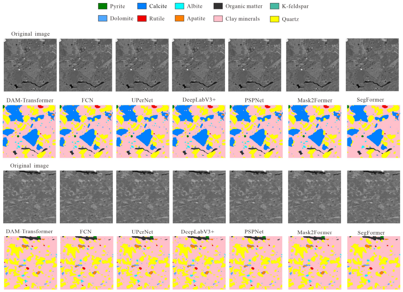
To compare the segmentation performance of the different methods, two samples containing all ten mineral classes in the ground truth annotations were selected for visual analysis. These samples included large clay mineral, quartz, and calcite regions, as well as small-scale pyrite, rutile, apatite, feldspar, and organic matter targets, enabling evaluation of multi-scale mineral identification and complex boundary delineation.

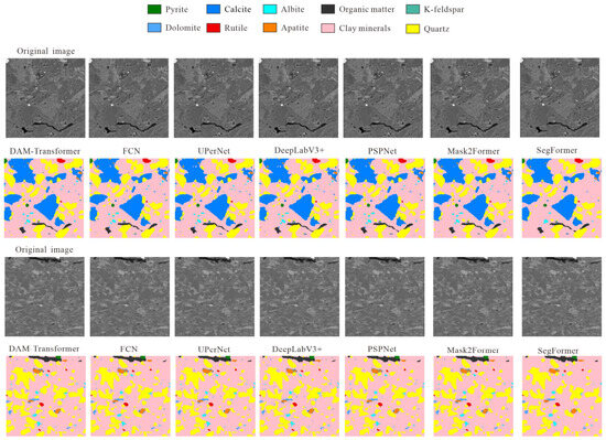
All methods produced broadly consistent segmentation maps for the dominant clay-mineral, quartz, and calcite regions, but clear differences appeared in the delineation of small mineral particles, fracture-like organic matter, boundary continuity, and local noise (Figure 10). The DAM-Transformer better preserved the outlines of large mineral regions while retaining scattered fine-grained minerals and narrow organic matter features. FCN tended to produce locally fragmented boundaries because of its reliance on convolutional local features. UPerNet improved the integrity of major regions through multi-scale feature fusion, but some confusion remained around fine-grained minerals. DeepLabV3+ and PSPNet recognized the main mineral distributions, but they more easily smoothed or omitted small and irregular targets. Mask2Former and SegFormer also captured the overall mineral pattern, but their predictions showed local deviations in minor minerals and boundary details. These visual comparisons indicate that the dynamic attention mechanism helps the DAM-Transformer adjust its receptive focus according to mineral texture and matrix background, thereby improving detail preservation in complex shale SEM images.

Figure 10. Comparison of visual identification results.

The generalization capability of DAM-Transformer mainly benefits from its mechanism-oriented design. The shifted-window attention structure extracts local textures, grain boundaries, mineral contact relationships, and matrix background features, while the shifted-window operation enables information exchange between adjacent regions. These features are not unique to shale but are also common in sandstone, carbonate rocks, and other sedimentary rocks. Therefore, DAM-Transformer can theoretically capture shared mineral texture and boundary features across different reservoir rocks.

In addition, the dynamic attention mechanism adaptively adjusts attention weights according to the input image features, allowing the model to focus on mineral regions, grain edges, pore–mineral contacts, and irregular boundaries. The hybrid loss function further reduces the dominance of high-abundance minerals and strengthens the recognition of fine-grained or low-abundance components. Therefore, under similar SEM imaging conditions, DAM-Transformer is expected to show good adaptability for mineral segmentation in sandstone, carbonate rocks, and other formations.

5. Application

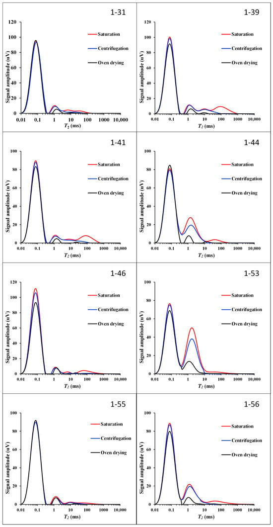
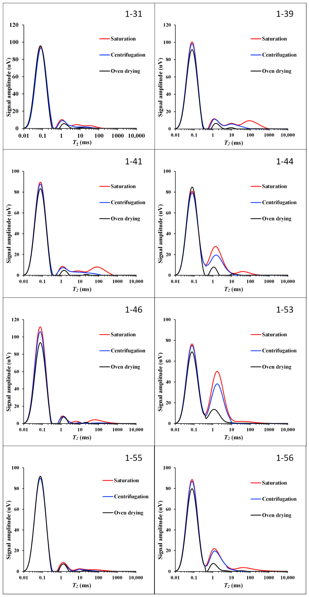
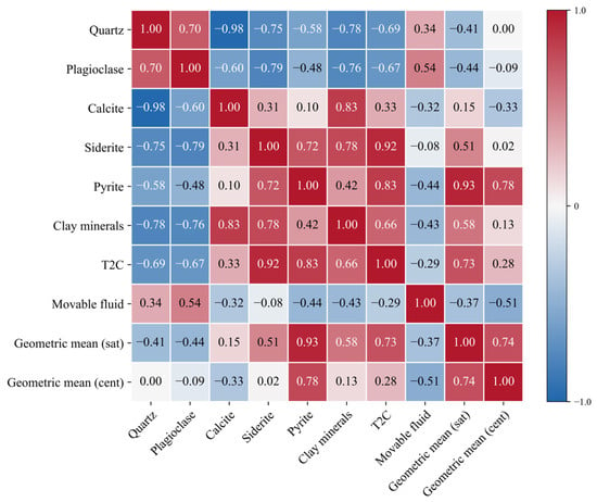
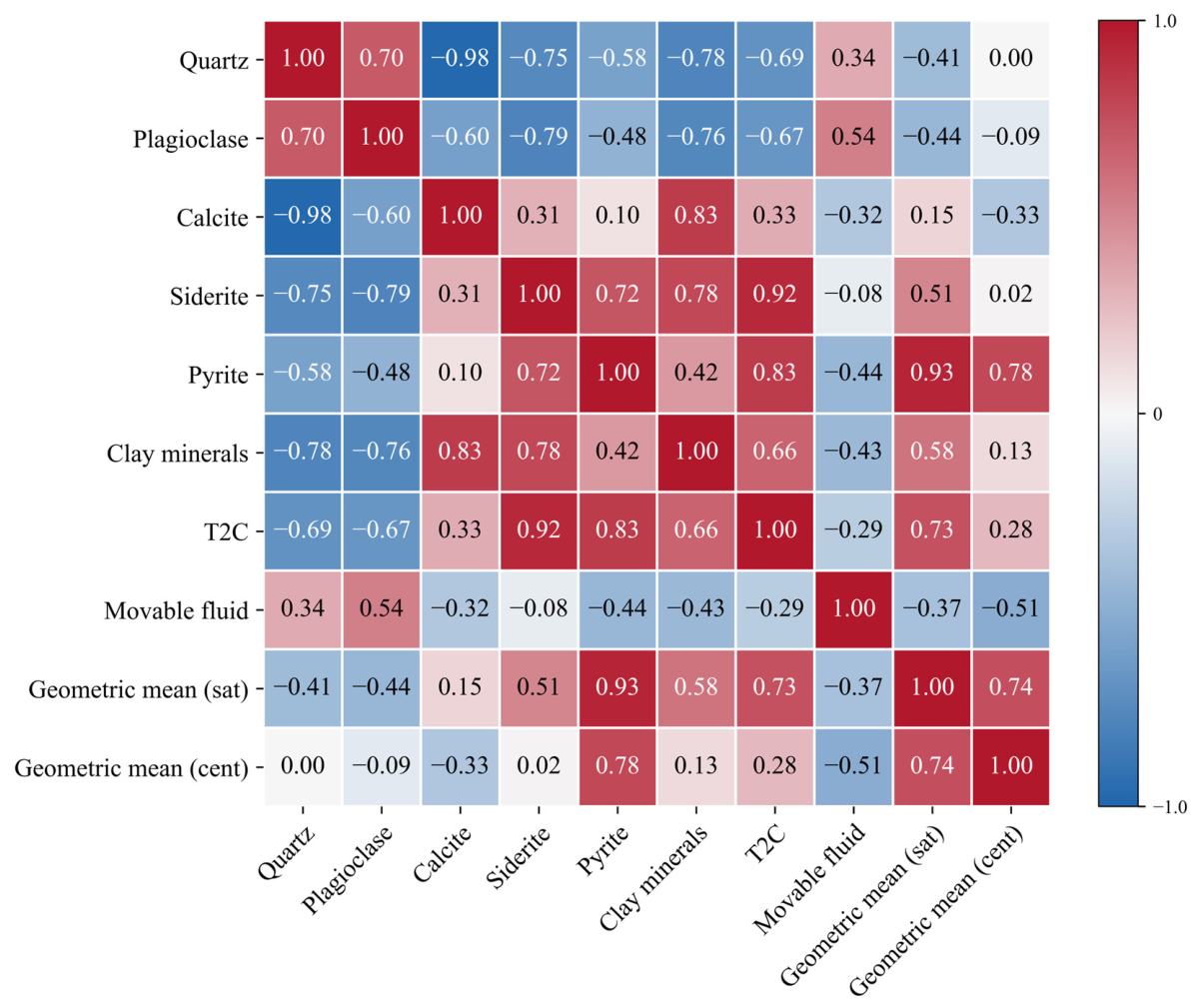
Based on DAM-Transformer mineral identification (Table 7) and saturation–centrifugation NMR parameters (Table 8) from eight shale samples (Figure 11), this study examined mineral–NMR relationships. The parameters included T2C (movable–bound fluid pore size boundary), movable fluid content, saturated geometric mean, and centrifuged geometric mean. The results showed that clay minerals, siderite, and pyrite generally correlated positively with T2C and geometric means, while quartz and plagioclase correlated negatively (Figure 12), indicating that mineral composition shapes pore structure, fluid occurrence, and residual fluid distribution.

Table 7. Mineral content of different samples.

Sample No.	Quartz (%)	Albite (%)	K-Feldspar (%)	Calcite (%)	Dolomite (%)	Apatite (%)	Clay Minerals (%)	Rutile (%)	Pyrite (%)	Organic Matter (%)
1-31	47.4	1.7	1.6	0.5	1.3	0.0	46.3	0.4	0.3	0.5
1-39	36.6	0.1	0.6	0.1	0.1	0.0	61.1	0.5	0.0	0.9
1-41	20.9	0.1	0.1	11.9	0.1	0.3	64.4	0.5	1.3	0.4
1-44	35.0	0.1	0.9	0.1	0.2	0.3	57.8	1.1	3.3	1.1
1-46	25.2	0.0	0.0	12.1	0.0	0.0	58.1	0.3	3.7	0.5
1-53	28.6	0.0	0.0	12.0	0.1	0.3	58.0	0.1	0.8	0.0
1-55	35.7	5.9	3.0	0.1	5.6	1.9	47.2	0.3	0.3	0.0
1-56	18.7	0.3	0.0	0.3	0.6	0.5	77.9	0.5	0.1	1.0

Table 8. One-dimensional NMR response characteristics of different samples.

Sample No.	T2C (ms)	Movable Fluid (%)	Gm (Sat)	Gm (Cent)
1-31	4.6	62.43	4.94	2.63
1-39	22	46.75	21.79	5.22
1-41	22	48.38	20.44	5.15
1-44	2	45.63	2.44	1.72
1-46	7.2	50.05	25.77	8.79
1-53	2	50.35	2.51	2.05
1-55	4.64	43.18	11.37	9.08
1-56	3.5	63.77	4.45	1.84

Figure 11. One dimensional NMR T2 spectra of different samples.

Figure 12. Heatmap of the correlations between mineral components and NMR parameters.

The results for quartz (T2C: −0.69; saturated geometric mean: −0.41) and plagioclase (−0.67 and −0.44) suggest that a higher felsic content lowers the T2 spectral center, likely as rigid grains dilute clay- or iron-mineral-related micropore contributions. Calcite showed weak positive correlations with T2C and saturated geometric mean (0.33 and 0.15) but negative correlations with movable fluid content and centrifuged geometric mean (−0.32 and −0.33), reflecting complex effects possibly tied to pore filling or cementation. Siderite showed the strongest T2C correlation (0.92) and a positive saturated geometric mean correlation (0.51), suggesting that it shifts the T2 spectrum toward longer relaxation times. Pyrite showed strong positive correlations with T2C and saturated and centrifuged geometric means (0.83, 0.93, and 0.78), making it most closely linked to NMR responses, possibly reflecting greater pore heterogeneity. Clay minerals correlated positively with T2C and saturated geometric mean (0.66, 0.58) but negatively with movable fluid content (−0.43), favoring bound fluid storage while reducing mobility. Organic matter showed weak correlations overall (T2C: 0.11; saturated geometric mean: −0.03; movable fluid: 0.22), indicating limited influence.

Because the mineral NMR correlation analysis was based on only eight shale plug samples, the inferred relationships should be treated as exploratory trends rather than definitive conclusions. Pearson correlation coefficients were evaluated alongside two-tailed significance tests, with 95% confidence intervals estimated via Fisher’s z transformation. With n = 8, there are only six degrees of freedom, meaning that only relatively strong correlations will reach significance and, thus, both the coefficient magnitude and statistical uncertainty must be considered.

Several correlations proved statistically meaningful: siderite with T2C (r = 0.92, p = 0.0012, 95% CI: 0.61–0.99), and pyrite with the saturated geometric mean (r = 0.93, p = 0.0008, 95% CI: 0.65–0.99), T2C (r = 0.83, p = 0.0108, 95% CI: 0.30–0.97), and the centrifuged geometric mean (r = 0.78, p = 0.0224, 95% CI: 0.17–0.96). These results indicate that iron-bearing minerals, especially siderite and pyrite, are closely linked to NMR responses. In contrast, the quartz–T2C (r = −0.69, p = 0.0582), plagioclase–T2C (r = −0.67, p = 0.0691), and clay–T2C (r = 0.66, p = 0.0749) correlations did not reach the 0.05 significance level and should only be viewed as potential trends.

The small sample size increases estimation uncertainty and sensitivity to individual samples. Thus, the reported mineral NMR relationships mainly reveal potential controlling trends, offering a quantitative basis for interpreting shale pore structure and fluid occurrence; future studies should increase the sample size and incorporate permeability, porosity, XRD, and other independent petrophysical measurements for validation. Regression modeling was not performed, as eight samples are insufficient to build a stable multivariate model involving multiple mineral components and NMR parameters; under such small-sample conditions, regression coefficients could be strongly skewed by individual samples, risking overinterpretation.

In summary, the influence of minerals on NMR parameters is mainly reflected in the following patterns: iron-bearing minerals and clay minerals enhance T2C and geometric mean responses, whereas clay minerals tend to suppress fluid mobility; felsic minerals generally reduce T2C and the saturated geometric mean. These results demonstrate that the mineral contents identified by the DAM-Transformer can provide a quantitative basis for interpreting differences in shale pore structure and fluid occurrence characteristics.

The influence of minerals on NMR responses depends not only on their abundance but also on the formation’s pore structure, connectivity, and fluid occurrence. T2C reflects the pore size boundary between movable and bound fluids, while the geometric mean characterizes the central tendency of the relaxation time distribution. Longer relaxation times generally indicate greater effective pore–throat contribution or improved connectivity, whereas shorter times relate to micropores, bound fluids, and isolated pores.

Clay minerals correlated positively with T2C and the saturated geometric mean but negatively with movable fluid content, suggesting that they promote micropore and bound fluid space development without necessarily improving connectivity. Their high specific surface area and layered structure enhance surface relaxation and fluid retention, boosting storage-related responses while reducing mobility (“improved storage, not flow capacity”). Iron-bearing minerals (siderite and pyrite) showed strong positive correlations with T2C and geometric means, likely linked to heterogeneous pore systems, mineral contact boundaries, or microfractures. Pyrite’s positive correlation with the centrifuged geometric mean suggests that there is residual fluid in relatively well-connected pores. In contrast, quartz and plagioclase correlated negatively with T2C and the saturated geometric mean, indicating that a higher felsic content does not necessarily enhance effective storage and may dilute the contribution of clay- or iron-mineral-associated pore systems.

Therefore, mineral effects on reservoir quality should be evaluated not just based on abundance; whether the mineral-associated pores are connected, whether the fluids are movable, and whether effective pore–throat pathways exist should be considered. Recent NMR studies support using such responses to characterize pore connectivity and fluid migration in porous media. For example, Hosseini [46] used borehole NMR to monitor raffinate flow and pore-connectivity evolution in heap-leach waste rock, offering a useful reference for linking NMR responses to connectivity and flow dynamics. The mineral NMR relationships identified here further support the interpretation of shale pore network connectivity and reservoir flow behaviors based on NMR responses.

6. Conclusions

• The DAM-Transformer enables whole-rock mineral component identification in shale SEM images. It simultaneously identifies matrix and associated minerals within a single SEM image and generates pixel-level mineral distribution maps, thereby achieving comprehensive mineral component coverage.
• The DAM-Transformer outperformed Mask2Former, FCN, UPerNet, DeepLabV3+, SegFormer, and PSPNet. It achieved an mAcc of 78.12%, mIoU of 69.27%, and mDice of 84.07%, representing average improvements of 5.54, 3.64, and 3.86 percentage points, respectively, over the benchmark methods.
• The dynamic attention mechanism and hybrid loss function jointly improve mineral identification performance. Dynamic attention adaptively distinguishes mineral targets from the matrix background, whereas the hybrid loss function reduces the dominance of extensive mineral classes during training. Together, they enhance the identification of fine-grained minerals, fracture-like organic matter, and complex boundaries.
• Clay minerals, siderite, and pyrite show relatively strong positive correlations with T2C and geometric mean values, whereas quartz and plagioclase are generally negatively correlated with T2C and the saturated geometric mean. This indicates that variations in mineral composition can influence shale pore structure, fluid occurrence state, and movable fluid characteristics.

References

- Hou, L.-H.; Wu, S.-T.; Jing, Z.-H.; Jiang, X.-H.; Yu, Z.-C.; Hua, G.-L.; Su, L.; Yu, C.; Liao, F.-R.; Tian, H. Effects of Types and Content of Clay Minerals on Reservoir Effectiveness for Lacustrine Organic Matter Rich Shale. Fuel 2022, 327, 125043. [Google Scholar] [CrossRef] [Scilit]
- Iqbal, M.A.; Rezaee, R.; Smith, G.; Ekundayo, J.M. Shale Lithofacies Controls on Porosity and Pore Structure: An Example from Ordovician Goldwyer Formation, Canning Basin, Western Australia. J. Nat. Gas. Sci. Eng. 2021, 89, 103888. [Google Scholar] [CrossRef] [Scilit]
- Chen, S.; Han, Y.; Fu, C.; Zhang, H.; Zhu, Y.; Zuo, Z. Micro and Nano-Size Pores of Clay Minerals in Shale Reservoirs: Implication for the Accumulation of Shale Gas. Sediment. Geol. 2016, 342, 180–190. [Google Scholar] [CrossRef] [Scilit]
- Kang, Y.; Zhu, R.; Liu, K.; Zhang, J.; Zhang, S. Detrital and Authigenic Clay Minerals in Shales: A Review on Their Identification and Applications. Heliyon 2024, 10, e39239. [Google Scholar] [CrossRef] [Scilit] [PubMed]
- Wu, Y.; Misra, S.; Sondergeld, C.; Curtis, M.; Jernigen, J. Machine Learning for Locating Organic Matter and Pores in Scanning Electron Microscopy Images of Organic-Rich Shales. Fuel 2019, 253, 662–676. [Google Scholar] [CrossRef] [Scilit]
- Liu, Y.; Wang, X.; Zhang, Z.; Deng, F. Deep Learning in Image Segmentation for Mineral Production: A Review. Comput. Geosci. 2023, 180, 105455. [Google Scholar] [CrossRef] [Scilit]
- Li, C.; Wang, D.; Kong, L. Application of Machine Learning Techniques in Mineral Classification for Scanning Electron Microscopy–Energy Dispersive X-Ray Spectroscopy (SEM-EDS) Images. J. Pet. Sci. Eng. 2021, 200, 108178. [Google Scholar] [CrossRef] [Scilit]
- Chen, Z.; Liu, X.; Yang, J.; Little, E.C.; Zhou, Y. Deep Learning-Based Method for SEM Image Segmentation in Mineral Characterization, an Example from Duvernay Shale Samples in Western Canada Sedimentary Basin. Comput. Geosci. 2020, 138, 104450. [Google Scholar] [CrossRef] [Scilit]
- Bihani, A.; Daigle, H.; Santos, J.E.; Landry, C.; Prodanović, M.; Milliken, K. MudrockNet: Semantic Segmentation of Mudrock SEM Images through Deep Learning. Comput. Geosci. 2022, 158, 104952. [Google Scholar] [CrossRef] [Scilit]
- Yin, B.; Hu, Q.; Zhu, Y.; Zhao, C.; Zhou, K. Paw-Net: Stacking Ensemble Deep Learning for Segmenting Scanning Electron Microscopy Images of Fine-Grained Shale Samples. Comput. Geosci. 2022, 168, 105218. [Google Scholar] [CrossRef] [Scilit]
- Yin, B.; Hu, Q.; Zhu, Y.; Zhou, K. Semi-Supervised Learning for Shale Image Segmentation with Fast Normalized Cut Loss. Geoenergy Sci. Eng. 2023, 229, 212039. [Google Scholar] [CrossRef] [Scilit]
- Yasin, Q.; Liu, B.; Sun, M.; Sohail, G.M.; Ismail, A.; Majdanski, M.; Golsanami, N.; Ma, Y.; Fu, X. Automatic Pore Structure Analysis in Organic-Rich Shale Using FIB-SEM and Attention U-Net. Fuel 2024, 358, 130161. [Google Scholar] [CrossRef] [Scilit]
- Li, B.; Nie, X.; Cai, J.; Zhou, X.; Wang, C.; Han, D. U-Net Model for Multi-Component Digital Rock Modeling of Shales Based on CT and QEMSCAN Images. J. Pet. Sci. Eng. 2022, 216, 110734. [Google Scholar] [CrossRef] [Scilit]
- Sun, P.; Ge, L.; Liu, Y.; Li, B.; Nie, X. Modeling of Multi-Mineral-Component Digital Core Based on Res-Unet. J. Geophys. Eng. 2023, 20, 483–493. [Google Scholar] [CrossRef] [Scilit]
- Liang, J.; Sun, Y.; Lebedev, M.; Gurevich, B.; Nzikou, M.; Vialle, S.; Glubokovskikh, S. Multi-Mineral Segmentation of Micro-Tomographic Images Using a Convolutional Neural Network. Comput. Geosci. 2022, 168, 105217. [Google Scholar] [CrossRef] [Scilit]
- Wang, Y.D.; Shabaninejad, M.; Armstrong, R.T.; Mostaghimi, P. Deep Neural Networks for Improving Physical Accuracy of 2D and 3D Multi-Mineral Segmentation of Rock Micro-CT Images. Appl. Soft Comput. 2021, 104, 107185. [Google Scholar] [CrossRef] [Scilit]
- Niu, Y.; Mostaghimi, P.; Shabaninejad, M.; Swietojanski, P.; Armstrong, R.T. Digital Rock Segmentation for Petrophysical Analysis with Reduced User Bias Using Convolutional Neural Networks. Water Resour. Res. 2020, 56, e2019WR026597. [Google Scholar] [CrossRef] [Scilit]
- Karimpouli, S.; Tahmasebi, P. Segmentation of Digital Rock Images Using Deep Convolutional Autoencoder Networks. Comput. Geosci. 2019, 126, 142–150. [Google Scholar] [CrossRef] [Scilit]
- Phan, J.; Ruspini, L.C.; Lindseth, F. Automatic Segmentation Tool for 3D Digital Rocks by Deep Learning. Sci. Rep. 2021, 11, 19123. [Google Scholar] [CrossRef] [Scilit] [PubMed]
- Cao, D.; Ji, S.; Cui, R.; Liu, Q. Multi-Task Learning for Digital Rock Segmentation and Characteristic Parameters Computation. J. Pet. Sci. Eng. 2022, 208, 109202. [Google Scholar] [CrossRef] [Scilit]
- Alqahtani, N.J.; Niu, Y.; Wang, Y.D.; Chung, T.; Lanetc, Z.; Zhuravljov, A.; Armstrong, R.T.; Mostaghimi, P. Super-Resolved Segmentation of X-Ray Images of Carbonate Rocks Using Deep Learning. Transp. Porous Media 2022, 143, 497–525. [Google Scholar] [CrossRef] [Scilit]
- Saxena, N.; Day-Stirrat, R.J.; Hows, A.; Hofmann, R. Application of Deep Learning for Semantic Segmentation of Sandstone Thin Sections. Comput. Geosci. 2021, 152, 104778. [Google Scholar] [CrossRef] [Scilit]
- Filippo, M.P.; Gomes, O.d.F.M.; da Costa, G.A.O.P.; Mota, G.L.A. Deep Learning Semantic Segmentation of Opaque and Non-Opaque Minerals from Epoxy Resin in Reflected Light Microscopy Images. Miner. Eng. 2021, 170, 107007. [Google Scholar] [CrossRef] [Scilit]
- Latif, G.; Bouchard, K.; Maitre, J.; Back, A.; Bédard, L.P. Deep-Learning-Based Automatic Mineral Grain Segmentation and Recognition. Minerals 2022, 12, 455. [Google Scholar] [CrossRef] [Scilit]
- Dong, L.; Gui, H.; Yu, X.; Zhang, X.; Xu, M. High-Accuracy Image Segmentation Based on Hybrid Attention Mechanism for Sandstone Analysis. Minerals 2024, 14, 544. [Google Scholar] [CrossRef] [Scilit]
- Zheng, D.; Hou, L.; Hu, X.; Hou, M.; Dong, K.; Hu, S.; Teng, R.; Ma, C. Sediment Grain Segmentation in Thin-Section Images Using Dual-Modal Vision Transformer. Comput. Geosci. 2024, 191, 105664. [Google Scholar] [CrossRef] [Scilit]
- Koeshidayatullah, A.; Ferreira-Chacua, I.; Li, W. Is Attention All Geosciences Need? Advancing Quantitative Petrography with Attention-Based Deep Learning. Comput. Geosci. 2023, 181, 105466. [Google Scholar] [CrossRef] [Scilit]
- Hassan, S.M.; Laban, N.; Abo Khashaba, S.M.; El-Shibiny, N.H.; Bashir, B.; Azer, M.K.; Drüppel, K.; Keshk, H.M. Semantic Segmentation of Some Rock-Forming Mineral Thin Sections Using Deep Learning Algorithms: A Case Study from the Nikeiba Area, South Eastern Desert, Egypt. Remote Sens. 2024, 16, 2276. [Google Scholar] [CrossRef] [Scilit]
- Knaup, A.; Jernigen, J.; Curtis, M.; Devegowda, D.; Sondergeld, C.; Rai, C. Application of Deep Learning to Shale Microstructure Classification. Mar. Pet. Geol. 2022, 144, 105842. [Google Scholar] [CrossRef] [Scilit]
- Xie, E.; Wang, W.; Yu, Z.; Anandkumar, A.; Alvarez, J.M.; Luo, P. SegFormer: Simple and Efficient Design for Semantic Segmentation with Transformers. Adv. Neural Inf. Process. Syst. 2021, 34, 12077–12090. [Google Scholar]
- Cheng, B.; Misra, I.; Schwing, A.G.; Kirillov, A.; Girdhar, R. Masked-Attention Mask Transformer for Universal Image Segmentation. In Proceedings of the IEEE/CVF Conference on Computer Vision and Pattern Recognition; IEEE: New York, NY, USA, 2022; pp. 1290–1299. [Google Scholar]
- Kirillov, A.; Mintun, E.; Ravi, N.; Mao, H.; Rolland, C.; Gustafson, L.; Xiao, T.; Whitehead, S.; Berg, A.C.; Lo, W.Y.; et al. Segment Anything. In Proceedings of the IEEE/CVF International Conference on Computer Vision; IEEE: New York, NY, USA, 2023; pp. 4015–4026. [Google Scholar]
- Yuan, Y.; Fu, R.; Huang, L.; Lin, W.; Zhang, C.; Chen, X.; Wang, J. HRFormer: High-Resolution Transformer for Dense Prediction. Adv. Neural Inf. Process. Syst. 2021, 34, 7281–7293. [Google Scholar]
- Wang, W.; Dai, J.; Chen, Z.; Huang, Z.; Li, Z.; Zhu, X.; Hu, X.; Lu, T.; Lu, L.; Li, H.; et al. InternImage: Exploring Large-Scale Vision Foundation Models with Deformable Convolutions. In Proceedings of the IEEE/CVF Conference on Computer Vision and Pattern Recognition; IEEE: New York, NY, USA, 2023; pp. 14408–14419. [Google Scholar]
- Ren, Y.; Li, X.; Bi, J.; Zhang, Y.; Su, Q.; Wang, W.; Li, H. Multi-Channel Attention Transformer for Rock Thin-Section Image Segmentation. J. Eng. Res. 2025, 13, 730–740. [Google Scholar] [CrossRef] [Scilit]
- Fan, J.; Yu, X.; Di, Y.; Lv, T.; Zhang, R.; Bao, J.; Liu, Y.; Li, L.; Pan, X. A Foundation Model for Rock Thin-Section Images Analysis. Commun. Eng. 2025, 5, 9. [Google Scholar] [CrossRef] [Scilit] [PubMed]
- Vaswani, A.; Shazeer, N.; Parmar, N.; Uszkoreit, J.; Jones, L.; Gomez, A.N.; Kaiser, Ł.; Polosukhin, I. Attention Is All You Need. Adv. Neural Inf. Process. Syst. 2017, 30, 5998–6008. [Google Scholar]
- Su, Z.; Zhou, G.; Luo, F.; Li, S.; Ma, K.-K. Semantic Segmentation of 3D Point Clouds Based on High Precision Range Search Network. Remote Sens. 2022, 14, 5649. [Google Scholar] [CrossRef] [Scilit]
- Jaccard, P. The Distribution of the Flora in the Alpine Zone. New Phytol. 1912, 11, 37–50. [Google Scholar] [CrossRef] [Scilit]
- Dice, L.R. Measures of the Amount of Ecologic Association Between Species. Ecology 1945, 26, 297–302. [Google Scholar] [CrossRef] [Scilit]
- Liu, Z.; Lin, Y.; Cao, Y.; Hu, H.; Wei, Y.; Zhang, Z.; Lin, S.; Guo, B. Swin Transformer: Hierarchical Vision Transformer Using Shifted Windows. In Proceedings of the IEEE/CVF International Conference on Computer Vision; IEEE: New York, NY, USA, 2021; pp. 10012–10022. [Google Scholar] [CrossRef] [Scilit]
- Long, J.; Shelhamer, E.; Darrell, T. Fully Convolutional Networks for Semantic Segmentation. In Proceedings of the IEEE Conference on Computer Vision and Pattern Recognition; IEEE: New York, NY, USA, 2015; pp. 3431–3440. [Google Scholar] [CrossRef] [Scilit]
- Xiao, T.; Liu, Y.; Zhou, B.; Jiang, Y.; Sun, J. Unified Perceptual Parsing for Scene Understanding. In Computer Vision—ECCV 2018; Springer: Berlin/Heidelberg, Germany, 2018; pp. 418–434. [Google Scholar] [CrossRef] [Scilit]
- Chen, L.-C.; Zhu, Y.; Papandreou, G.; Schroff, F.; Adam, H. Encoder-Decoder with Atrous Separable Convolution for Semantic Image Segmentation. In Computer Vision—ECCV 2018; Springer: Berlin/Heidelberg, Germany, 2018; pp. 801–818. [Google Scholar] [CrossRef] [Scilit]
- Zhao, H.; Shi, J.; Qi, X.; Wang, X.; Jia, J. Pyramid Scene Parsing Network. In Proceedings of the IEEE Conference on Computer Vision and Pattern Recognition; IEEE: New York, NY, USA, 2017; pp. 2881–2890. [Google Scholar] [CrossRef] [Scilit]
- Hosseini, M. In-situ Monitoring of Raffinate Flow and Pore Connectivity Evolution in Heap Leach Waste Rock Using Borehole Magnetic Resonance. Hydrometallurgy 2026, 244, 106806. [Google Scholar] [CrossRef] [Scilit]
Disclaimer/Publisher’s Note: The statements, opinions and data contained in all publications are solely those of the individual author(s) and contributor(s) and not of MDPI and/or the editor(s). MDPI and/or the editor(s) disclaim responsibility for any injury to people or property resulting from any ideas, methods, instructions or products referred to in the content. |
© 2026 by the authors. Licensee MDPI, Basel, Switzerland. This article is an open access article distributed under the terms and conditions of the Creative Commons Attribution (CC BY) license.