


Highlights
What are the main findings?
- •
- Sequential backward band selection (GPR-BAT) achieved accuracy comparable to PCA for N uptake and NNI using only two or three bands, while PCA performed better for AGB.
- •
- Key bands clustered in NIR for all traits, red-edge for N uptake and NNI, and blue for NNI, giving models more interpretable than PCA.
What are the implications of the main findings?
- •
- Band selection avoids acquiring the full hyperspectral cube, cutting data, computing, and cost barriers to on-farm N monitoring.
- •
- The selected spectral regions define two candidate multispectral sensors for precision N management to be validated with real sensors.
Abstract
Hyperspectral imaging adoption is hindered by high investment costs, and multicollinearity among contiguous bands requires dimensionality-reduction (DR) algorithms, raising concerns about cost-effectiveness for farmers. In this study, we propose a direct comparison between feature extraction and feature selection methods as DR strategies for monitoring the nitrogen (N) status of processing tomato. The hyperspectral reflectance (399–1001 nm) was monitored in a processing tomato experiment with four N levels alongside crop traits (aboveground biomass, AGB; N uptake; N nutrition index, NNI). Gaussian process regression (GPR) was trained in two DR scenarios, (i) feature extraction using principal component analysis (GPR-PCA) and (ii) feature selection, with a sequential backward band removal (band analysis tool, BAT, in ARTMO software (v3.30); GPR-BAT), to identify the most informative key bands. The GPR-PCA achieved the highest mean accuracy for AGB, whereas for N uptake and NNI GPR-BAT yielded comparable estimation performance. Selected bands were located in the NIR for all variables, in the red-edge for N uptake and NNI, and in the blue region for NNI, and were interpreted as candidate spectral regions. Based on the identified bands, two candidate multispectral sensor configurations were proposed for N monitoring: an AGB–NNI scenario (6 bands) and an AGB–N uptake scenario (5 bands). These findings suggest the potential of task-specific multispectral sensors for crop N monitoring, although NNI accuracy (RMSE ≈ 0.11 NNI units) remains insufficient for decisions close to the fertilization threshold.
1. Introduction
Nitrogen (N) fertilization represents one of the major environmental burdens in processing tomato cultivation [1] due to nitrate leaching into groundwater and the emission of nitrous oxide, a greenhouse gas (GHG) nearly 300 times more impactful than CO2. The N fertilizer supply chain is therefore a major source of GHG emissions, as shown by Menegat et al. [2], who attributed 10.6% of global agricultural GHG emissions to the N fertilizer sector, corresponding to 2.1% of total global emissions. Reducing N inputs is indeed critical to achieve a more sustainable and resilient agricultural sector, and digital agriculture is a direct strategy to optimize the use of mineral fertilizers and meet actual crop N demand. Monitoring crop N status with digital tools (e.g., chlorophyll meters, reflectance sensors) enables dynamic adjustment of fertilization using a speaking-plant approach [3], resulting in a reduction in N fertilizer use of up to 60% [4]. In recent decades, optical sensors have become increasingly popular for their rapid, large-scale, and non-destructive monitoring of crops, and among these, hyperspectral sensors are particularly relevant in the remote sensing community. By capturing reflectance across hundreds of narrow, contiguous spectral bands, hyperspectral imaging enables detection of subtle variations in crop biophysical traits, supporting precision agriculture applications [5].
Hyperspectral data have proven effective across multiple crop monitoring tasks. Cerasola et al. [6] used full-spectrum hyperspectral reflectance from processed tomato to retrieve biophysical traits (crop N uptake and biomass) in a machine learning framework and accurately estimated crop N demand (R2 = 0.86), reconstructing the critical N uptake curve. Similarly, Wang et al. [7] accurately estimated the leaf N content (LNC) employing the full hyperspectral spectrum in cereal crops. However, the main drawback of hyperspectral data is its very high dimensionality. Indeed, the adjacent narrow bands introduce redundancy by carrying similar information, which, if not addressed via dimensionality reduction (DR) techniques, may lead to suboptimal regression performance, often referred to as the curse of dimensionality [8]. Furthermore, end-users’ adoption is strongly hindered by the high investment costs of hyperspectral cameras [9]. Although open-access satellite missions (e.g., PRISMA, EnMAP, CHIME) provide free access, specialist skills in image post-processing and considerable computational and storage resources are still required. This conflicts with the limited digital literacy among EU farmers, which is a major barrier to the adoption of digital technologies [9]. The a priori preference for hyperspectral imaging has also been questioned by Matese et al. [10], especially when comparable performance can be achieved by multispectral, or even simple RGB sensors. Yet, in some cases, hyperspectral cameras were used to detect the nitrogen nutrition index (NNI) using only a few vegetation indices [11] or full-spectrum approaches [6,12], although multispectral sensors have also been shown to provide effective monitoring [13,14,15]. That said, in some instances, hyperspectral cameras are irreplaceable, as they provide highly informative data, enabling the detection of subtle changes that simpler multispectral sensors cannot. To this end, the early detection of Xylella fastidiosa before symptom appearance in olive trees [16] and the pre-symptomatic discrimination of early blight from late blight in potato [17] represent great examples.
Nowadays, DR can be achieved using two main approaches, feature extraction and feature selection [18], which encompass a wide range of algorithms. Briefly, feature extraction generates new variables by transforming the original bands, with principal component analysis (PCA) representing a widely used approach for high-dimensional data [19,20,21], excelling specifically when combined with machine learning algorithms [22]. PCA projects hyperspectral data onto a smaller set of uncorrelated principal components (PCs) [23], which can serve as input variables for estimating crop biophysical traits, thereby reducing noise and model complexity [22]. However, PCA reduces interpretability, because the contribution of individual bands to crop trait estimation is lost during the feature transformation [20,24]. Furthermore, since the transformation is applied to the full spectrum, acquiring the complete hyperspectral cube remains a prerequisite, leaving logistical and economic barriers unresolved, including data storage requirements and investment costs. From this perspective, working with a reduced set of task-optimized bands (e.g., multispectral sensors) may enable more efficient use of computational and economic resources, while ensuring equivalent estimation performance and accelerating post-processing workflows. In this perspective, feature selection methods, commonly categorized into filter, wrapper, and embedded approaches, identify a small subset of the most informative bands prior to model training. The original bands are preserved, avoiding any transformation that would limit model interpretability, though the band selection process itself may require considerable computational effort, depending on the algorithm employed [24]. For instance, Verrelst et al. [25] showed that hyperspectral data could be reduced to as few as nine and four bands to estimate leaf chlorophyll content and leaf area index (LAI), respectively, while Hassanzadeh et al. [26] employed feature selection in hyperspectral imaging to estimate bean yield, identifying just five decorrelated wavebands, with the goal of transferring their model to a low-cost multispectral system. Although the research community has acknowledged the benefits of more transparent and interpretable models, direct comparisons between feature extraction and selection approaches for crop trait retrieval remain limited, especially for N-related variables. To our knowledge, only Pascual-Venteo et al. [20] compared these two approaches using a PROSAIL-simulated dataset within a hybrid machine learning framework, finding that a model trained on 20 PCs outperformed a comparable model trained on the 20 best-ranked bands in retrieving several crop traits, including LAI. The authors noted, however, that the performance of both approaches could be further enhanced by individually optimizing the number of retained features.
Therefore, the objective of this study is to compare a feature extraction approach (PCA-based) with a feature selection approach based on the iterative least informative band removal [25], each under its individually optimized number of features, in monitoring crop N status by retrieving aboveground biomass (AGB), N uptake, and the NNI in processing tomato. Specifically, we aimed to: (i) compare the retrieval performance of Gaussian process regression (GPR) models based on the full spectrum, on principal component (GPR-PCA), and on the selected bands (GPR-BAT); (ii) identify the most informative spectral regions for each trait; (iii) evaluate candidate multispectral sensor configurations derived from the selected bands for N management.
2. Materials and Methods
2.1. Experimental Design and Crop Management
A plot-level field experiment was conducted from May to August 2023 at the experimental farm of the University of Bologna located in Cadriano in Northern Italy (44°32′58″ N, 11°24′37″ E; local climate Cfa according to the Köppen classification), where a processing tomato cultivar (K2206, ISI Sementi SpA, Fidenza, Italy) was transplanted in a single-row cropping system, with a distance between rows of 1 m, and a distance between plants in the same row of 0.36 m, resulting in a total of 27,778 plants ha−1. The experiment, described in detail in Cerasola et al. [6], is briefly summarized here. Four N fertilization levels were applied to the experimental plots, each 9 m × 5 m, arranged in a four-times-replicated complete randomized design, totaling 16 independent experimental units. The total crop N requirement was calculated using the N balance method [27], yielding 180 kg N ha−1, and N fertilizer was supplied via fertigation at 0, 20, 60, and 100% of total crop N requirements (0, 36, 108, and 180 kg N ha−1). Phosphorus was fully supplied at soil tillage at the rate of 80 kg P2O5 ha−1, while a total of 150 kg of K2O ha−1 was supplied through fertigation in three distinct moments along the growing season. Crop water requirements were met through drip irrigation, using the soil water balance method reported by Cerasola et al. [28].
2.2. Ground Data Measurements
At five growth stages (24, 30, 42, 49, and 55 days after transplant, DAT), aboveground crop traits (AGB, N uptake, and NNI) were monitored by sampling three plants, representing plant-level observation, per experimental unit (the 16 plots) at each date, for a total of 240 plants. Before plant collection, their coordinates were recorded for subsequent spatial referencing using a Topcon HiPer V GNSS system (Topcon Positioning Systems, Inc., Livermore, CA, USA, horizontal accuracy of 0.010 m and vertical accuracy of 0.015 m in RTK mode).
The fresh plant biomass was weighed with a precision scale. Each plant was oven-dried at 60 °C to a constant weight for dry plant biomass measurement. Subsequently, plant dry mass was converted to area-based AGB using the planting density. To determine the N uptake (kg N ha−1), the entire dried plants, including all plant organs (leaves, stems, and fruits), were ground into small pieces (2–5 mm), and a homogenized sub-sample was selected and further ball-milled into powder. Total N concentration (N%) was determined with a CHN elemental analyzer (Thermo Fisher, mod. EA 1110, Bremen, Germany). The N uptake was calculated as the product between the N concentration (%) and the dry mass per unit area (kg ha−1). The NNI was computed as the ratio of the N% monitored in the plant to the critical N%, derived from the AGB using the critical N dilution curve for processing tomato developed by Tei et al. [29]. The resulting crop traits measured at the plant level were finally averaged at the plot level.
2.3. Spectral Data Acquisition, Data Preprocessing, and Spectra Extraction Method
Spectral images were collected between 11:00 and 14:00 on the same day as ground data monitoring, when the sun was closest to the zenith during the growing season, in order to minimize shadowing and illumination effects, as previously demonstrated by Gianquinto et al. [15]. On each sampling date, all 16 plots were acquired with a single flight lasting approximately 8 min, given the small size of the experimental field (about 40 × 50 m), so that changes in solar zenith angle among plots were negligible. Images were captured at 40 m above the ground using the unmanned aerial vehicle (UAV) DJI Matrice 600 (DJI, Shenzhen, China) equipped with the hyperspectral camera Headwall Nano-Hyperspec® (Headwall Photonics Inc., Bolton, MA, USA). To minimize camera movement during flight, the camera was mounted on a stabilized Ronin MX Gimbal system (DJI, Shenzhen, China). The camera detected the incoming radiation between 399 and 1001 nm in 273 bands with a full width at half maximum (FWHM) of 6.6 nm, a sampling interval of 2.2 nm, and a ground sampling distance of 4 cm.
Spectral images were preprocessed as described in Cerasola et al. [6] using Headwall’s SpectralView software (Headwall Photonics Inc., Bolton, MA, USA), according to the sensor manual. Before each flight, the white and dark references were measured with the cap on the 12 mm lens (dark reference) and with a reference Spectralon® white panel (Labsphere, North Sutton, NH, USA) placed in the field of view of the sensor to obtain the gain and offset used for radiometric correction, and convert the digital numbers into radiance data. Reflectance was then calculated from radiance using a white calibration tarp placed on the soil within the imaged area during each flight, which accounted for the illumination conditions at the time of acquisition. Orthorectification was performed, and spatial alignment with the experimental plots was verified using QGIS.
The spectral signature of each plant was extracted from georeferenced raster images processed using custom Python software v3.11 (Python Software Foundation, Wilmington, DE, USA). The spatial coordinates of individual plants were first computed using the known plant spacing (1 m × 0.36 m) and the field boundary polygon, thereby generating a regular grid of theoretical plant positions within the study area. Observed plant coordinates, obtained from GNSS measurements, were then corrected using ground control points (GCPs), white panels in the field of view of the sensor georeferenced in the field before the flight, to account for systematic positional errors. The residual positional error after this correction, however, was not quantified. The corrected plant positions were subsequently matched to the theoretical grid by assigning each observation to the nearest plant position based on Euclidean distance, thereby minimizing residual spatial misalignment. Subsequently, a plant-specific bounding box was defined and sized according to the plant spacing, corresponding to the ground area allocated to a single plant (1 m × 0.36 m) and approximately 680 pixels at a ground sampling distance of 2.3 cm. Adjacent bounding boxes did not overlap, so that each pixel was assigned to a single plant. Although at later growth stages the canopies of neighboring plants could partially extend into the target bounding box, only the inner plants of the plot were sampled, excluding the borders. Therefore, neighboring plants belonged to the same plot and N treatment, and were expected to show similar canopy development and N status, preventing cross-contamination between treatments. Moreover, since spectra were averaged at the plot level (see below), the extracted signal represents the plot as an experimental unit rather than individual plants. The orientation of each bounding box was aligned with the crop row direction, determined from two reference plants with known coordinates. The line connecting these points defined the row direction, and the corresponding inclination angle was computed to rotate the bounding boxes. The bounding boxes were then used to clip the raster, and the median reflectance value for each wavelength was calculated within each bounding box. The extracted spectral signal intentionally included both vegetation and soil backgrounds, as no vegetation masking was applied, to reproduce mixed-pixel conditions and approximate the low spatial resolution of hyperspectral satellite observations. Consequently, the contribution of soil pixels was the highest during early growth stages and progressively decreased as canopy development progressed.
Of the 240 plant spectra theoretically available (16 plots × 3 plants × 5 sampling dates), 16 could not be extracted because the corresponding plots were partially cut at the edge of the hyperspectral image: one plant of treatment N0 at the second sampling date, and all plants of five plots at the fourth sampling date (belonging to all four N treatments). Since this depended on the image coverage rather than on plant characteristics, and all N treatments were affected, the excluded spectra were not expected to bias the analysis. Plant spectra from the same experimental unit (plot) and sampling date were then averaged, yielding 75 plot-level observations. In addition, eight bare-soil spectra were included in the AGB and N uptake datasets, with AGB and N uptake values set to zero, to represent non-vegetated conditions. Since NNI is a plant-based physiological index, bare-soil spectra were excluded from the NNI dataset. The final datasets, therefore, included 83 observations (75 plot-level + 8 bare-soil observations) for AGB and N uptake, and 75 vegetated plot-level observations for NNI. To assess whether bare-soil observations influenced the results, GPR-BAT was also retrained for AGB and N uptake, excluding bare-soil observations (n = 75), using the same selection criterion (Section 2.5). The selected spectral regions and accuracy were then compared with those obtained with bare soil included. The spectra were then smoothed using the Savitzky–Golay filter [30] in RStudio (version 4.2.0, Posit Software, PBC, Boston, MA, USA) with the signal package (polynomial order = 3, window size = 21 points), consistently with previous work on the same sensor and crop [6]. At the spectral edges, where a full 21-point window was not available, no padding was applied to avoid introducing artifacts from artificially extended values: as implemented by default in the sgolayfilt function of the signal package, the first and last ten bands were smoothed using the polynomial fitted to the first and last 21 measured bands. Smoothing was mainly required to reduce the high-frequency noise observed in the NIR region, while the third-order polynomial limited the distortion of the main spectral features of vegetation. Since adjacent wavelengths were already highly correlated, given the 2.2 nm sampling interval relative to the 6.6 nm FWHM, and smoothing tends to increase this correlation, the selected bands were interpreted as candidate spectral regions rather than specific wavelengths (Section 2.5).
2.4. Modeling and Validation Approach
Gaussian process regression (GPR, [31]) is a kernel-based and nonparametric Bayesian algorithm, and it was chosen in this paper as it was successfully adopted in previous studies for hyperspectral N-related variable monitoring [6,25,32,33,34] due to its excellent performance in modeling complex and nonlinear spectral data. GPR can capture the intricate functional relationship between input and output variables without making assumptions about their functional form. This algorithm has been primarily introduced in Earth observation studies as part of hybrid workflows that incorporate radiative transfer models [32,33], but it has also demonstrated strong performance in classic machine learning workflows [6]. In addition to its predictive performance, GPR’s Bayesian nature and probabilistic approach enable it to generate uncertainty estimates for the retrieved variable, a valuable metric for assessing the robustness and portability of a retrieval model under other conditions [35]. Given these properties, the GPR model was used as a benchmark algorithm after the two DR approaches were applied (feature extraction via PCA and feature selection via the Band Analysis Tool, further detailed in Section 2.5). GPR training and validation, as well as the DR method, were run with the Automated Radiative Transfer Models Operator (ARTMO) (https://artmotoolbox.com/, accessed on 26 October 2026) in MATLAB R2023a (The MathWorks, Inc., Natick, MA, USA). ARTMO includes a machine learning regression algorithm (MLRA) toolbox, allowing a variety of MLRAs to be selected and run via a graphical user interface, even in combination with multiple DR algorithms. In general, the performance of MLRAs depends on optimizing hyperparameters before model training, which is crucial for preventing overfitting and high prediction error. GPR models were implemented using a squared-exponential covariance function with automatic relevance determination (ARD; covSEardj), combined with an independent Gaussian noise covariance (covNoise). Each input feature was assigned a separate length scale (σB), and initial values were set to the half of the observed range of each training feature; initial signal variance was set to the variance of the training targets, and initial noise variance to one quarter of that variance. The σB and signal/noise standard deviations were parametrized in logarithmic space. Hyperparameters were estimated by minimizing the negative log marginal likelihood using a Polak–Ribière nonlinear conjugate-gradient optimizer with polynomial line searches and Wolfe–Powell conditions. Optimization was limited to 100 objective function evaluations and could stop earlier if no further progress was possible. No explicit finite lower or upper hyperparameter bounds were imposed by the inspected implementation. The ARD covariance function also applied diagonal numerical jitter equal to 10−6 times the signal variance. All analyses were performed in ARTMO v3.30 running in MATLAB R2023a. In GPR-BAT, bands were ranked at each iteration by the sum of their σB rankings across the cross-validation folds (option “Ranking” for band sorting), removing one band per iteration, starting with the full spectrum (i.e., no bands were removed a priori in the first iteration).
The validation process involved a 4-fold cross-validation technique to limit overfitting [36]. This technique randomly splits the dataset into k = 4 equal-sized subsets; k − 1 subsets are used as training sets, and the remaining subset is used for model validation. This process is repeated k times, with each subset used for training and validation. Plot-level observations were randomly allocated by the ARTMO toolbox to four folds of approximately equal size, without stratification or grouping, and the same random partition was used for all modeling approaches (GPR-Full bands, GPR-PCA, and GPR-BAT), ensuring a paired comparison between them. Since each observation corresponds to one plot at one sampling date, observations of the same plot collected at different sampling dates could be assigned to different folds. Although these observations differed markedly in canopy development and reflectance across sampling dates, they were not statistically independent because repeated measurements of the same plot shared its N treatment, replicate, and soil. Because the same plot could contribute observations to both training and validation folds, the validation set was not fully independent, and the absolute R2 and NRMSE values may be optimistic for predictions on new plots, whereas the paired comparison among approaches is less affected.
This resampling approach is particularly suited to small datasets, where holding out a single fixed test set would either sacrifice a substantial share of the calibration data or yield performance estimates strongly dependent on the specific partition; by averaging the error across folds, k-fold cross-validation mitigates this dependence and provides a more reliable accuracy estimate than a single train–test split. For this reason, k-fold cross-validation is an established validation strategy in studies addressing nitrogen-status retrieval from spectral imagery under limited dataset size [37,38,39]. As the dataset was collected within a single growing season, the cross-validated metrics reflect predictive performance within the sampled range of conditions and do not establish transferability across years and environments. It should be noted, however, that the aim of this work is not to certify the absolute accuracy of a single retrieval model, but to compare two hyperspectral dimensionality-reduction strategies (detailed in Section 2.5) for estimating nitrogen status under an identical evaluation protocol, i.e., on the same cross-validation folds. In GPR-BAT, bands were ranked using only the models trained on the training folds. However, the ranking was aggregated across folds, whose training sets include the validation observations of the other folds, and the numbers of PCs and bands were selected based on the same validation folds used to report accuracy. Since no nested cross-validation was performed, the reported accuracies are likely biased.
Fit validation statistics are averaged across the four validation subsets. In particular, the R2 and the relative root mean square error (NRMSE) are used as goodness-of-fit statistics.
where and are the observed and estimated variables, respectively, and and are the maximum and minimum values of the observed variable.
Additionally, the coefficient of variation (CV, %) provided along with the estimated variable from the GPR algorithm in the ARTMO toolbox is used to assess the uncertainty of the estimate.
where is the standard deviation estimated from the GPR algorithm of the i observation, and is the estimated variable of observation i.
All reported performance metrics and predictions refer to the validation folds (out-of-fold predictions); training performance is not reported, and no independent test set was available.
2.5. Dimensionality Reduction Techniques: The Two Approaches Compared
Two distinct DR strategies, namely feature extraction and feature selection, were compared using the hyperspectral dataset of processing tomato crop before training the GPR. The aim was to evaluate whether a limited set of optimally selected bands could achieve performance comparable to that of the widely adopted full-spectrum PCA approach. PCA is indeed a standard procedure in remote sensing and dimensionality-reduction tasks [6,19,20,21]. Furthermore, when combined with nonlinear machine learning algorithms, such as GPR, PCA was among the top-performing algorithms and reduced GPR uncertainty in the estimate [22]; therefore, it was chosen as a benchmark “feature extraction” algorithm. In PCA, the large number of spectral data is reduced to a restricted number of uncorrelated principal components (PCs) by applying a linear transformation to the original bands, which are used as input in the subsequent training stage of the GPR (GPR-PCA). The number of PCs that are included as input variables in GPR was selected as in Cerasola et al. [6]. First, GPR-PCA models were trained with increasing numbers of PCs (from 0, corresponding to the full spectrum without any reduction in the dimensionality, to 20), then the number of PCs was optimized following two sequential criteria: first, the minimum number of PCs explaining at least 99.5% of the spectral variance was identified. Then, starting from this number, the fold-averaged R2 and NRMSE curves were visually inspected: since the performance typically reached a plateau in which differences between consecutive numbers of PCs were small and likely due to random fluctuations, the number of PCs at which the performance plateau began was selected, i.e., the point beyond which additional PCs produced no consistent improvement in either metric. The resulting PCs were used as input data in a GPR algorithm to estimate AGB, N uptake, and NNI. The mathematical details of PCA are beyond the scope of this paper; we refer readers to Wold et al. [40] for further details.
In contrast, the “feature selection” strategy was implemented as a sequential backward band removal algorithm embedded in the Band Analysis Tool (BAT) of the ARTMO toolbox in MATLAB, as proposed by Verrelst et al. [25]. The BAT algorithm was used as a reference feature selection method, as it has been widely adopted in numerous studies [20,34,41,42,43,44]. The GPR-BAT procedure is essentially a sequential backward band-removal algorithm, a wrapper feature-selection method that uses the output of a regression algorithm to guide band selection and identify the most informative bands for crop trait retrieval [25]. In GPR-BAT, the correlation length σB for each spectral band of the GPR kernel function is used as an importance measure: the lower the σB, the higher the importance. At each iteration, the σB values of the GPR models trained on the training folds are ranked and aggregated across folds (Section 2.4), and the least informative bands, i.e., the bands with the highest aggregated rank, are removed. At each step, a new GPR model is automatically trained and validated using the remaining bands, and this process continues until only one band remains (Figure 1). For further details, the reader is referred to Verrelst et al. [25] and Pascual-Venteo et al. [20]. The same plateau criterion defined above for PCs’ selection was also adopted for GPR-BAT, without the variance threshold: the number of bands at which the plateau began along the sequential removal was selected, i.e., the point beyond which retaining additional bands produced no consistent improvement in either R2 or NRMSE. R2 and NRMSE indicated the same number of bands for all variables under both dimensionality reduction approaches. To assess whether the selection of bands at the spectral edges was driven by their lower signal-to-noise ratio, GPR-BAT was also repeated for all variables after excluding the first and last ten bands (i.e., using the 421–979 nm range), with the same data partition and selection criterion.
Figure 1.
Workflow of the analysis with the two DR approaches.
As a sensitivity check, the selection of both PCs and bands was compared with a quantitative one-standard-deviation (one-SD) rule, applied in three steps. First, the best model was identified separately for each metric, i.e., the model with the highest fold-averaged R2 and the model with the lowest fold-averaged NRMSE. Second, a threshold was derived for each metric from the best model and its fold-SD: the best R2 minus its SD, and the best NRMSE plus its SD. Third, among the models that met both thresholds, the one with the fewest features was selected and compared against the visual inspection criterion. For PCA, only the numbers of PCs explaining at least 99.5% of the variance were considered.
As a baseline, a GPR model trained on all available bands (GPR-Full bands) was also included for comparison.
To assess the stability of spectral region relevance across data partitions, the σB of the full-spectrum model (273 bands), corresponding to the first iteration of the GPR-BAT procedure, was extracted for each of the four cross-validation folds. Within each fold, wavelengths were ranked by increasing σB, and the ten most relevant bands with the lowest σB were identified. The selection frequency of each wavelength was then computed as the number of folds in which it ranked within the top ten (0–4), following the approach of Perich et al. [41]. Wavelengths were finally grouped into spectral regions (blue: 400–500 nm; red-edge: 700–750 nm; NIR: 750–1000 nm) to evaluate their stability and relevance. Since this analysis was based on the full-spectrum model, it assessed the stability of band relevance at the first iteration of GPR-BAT, and not the stability of the final bands selected by the sequential procedure. It was therefore used to identify the spectral regions consistently relevant across partitions, and the correspondence between the final bands and these regions was not intended to validate their stability.
3. Results
3.1. Dimensionality Reduction and Selection of Relevant Bands
The effect of the number of principal components on model performance is shown in Figure 2a,c. The relationship between the number of PCs and model performance was trait-dependent, with contrasting patterns among AGB, N uptake, and NNI. For NNI, increasing the number of PCs generally reduced model performance, as indicated by lower R2 and higher NRMSE values, with performance peaking at 5–10 PCs (Figure 2a,c). We therefore selected 5 PCs that maintained high performance while limiting model complexity. Conversely, for N uptake and AGB, the opposite trend was observed: model performance improved as the number of PCs increased, achieving stable top-performances at 12 PCs (Figure 2a,c). The one-SD rule confirmed the selected numbers of PCs for all variables.
Figure 2.
Performance of GPR validation models (R2 and NRMSE) as a function of the DR approach adopted: GPR-PCA (a,c), and in the sequential backward band removal GPR-BAT approach (b,d). In panels a and c, the vertical dashed lines indicate the minimum threshold (99.5%) of cumulative variance explained by the PCs. R2 and NRMSE are cross-validated metrics, averaged across the four validation folds.
The sequential backward band removal (GPR-BAT) identified compact subsets of informative wavelengths for all target variables. The optimal GPR-BAT models retained 3 bands for AGB and NNI, and 2 bands for N uptake, with both metrics giving the same optimum (Figure 3). The one-SD rule confirmed the selected number of bands for N uptake and NNI. For AGB, it indicated two bands (869 and 1001 nm) instead of three. In this case, the two metrics diverged: R2 indicated two bands, whereas NRMSE indicated one, owing to the large fold-SD of NRMSE (±3.16%), although the one-band model had a markedly lower R2 (0.795). The model with the smallest number of features meeting both the R2 and NRMSE thresholds included two bands, with slightly lower fold-averaged accuracy than the three-band model (R2 = 0.854 vs. 0.868; NRMSE = 12.80% vs. 12.10%; Table S1). The two criteria, therefore, led to very similar models. During the backward elimination process, model performance followed a consistent pattern: it improved or remained stable as redundant bands were removed, reached an optimum with a limited number of wavelengths, and then decreased sharply when further band removal discarded informative spectral regions (Figure 2b,d). This response was particularly evident for AGB and N uptake, where performance improvements became apparent once fewer than approximately 150 bands were retained. Conversely, when more than 150 bands were retained, band elimination produced little or no improvement, suggesting that a large portion of the hyperspectral dataset contained redundant information for trait retrieval.
Figure 3.
Position in the spectrum of the bands identified by the GPR-BAT sequential backward band removal for each N-related variable. The black and grey spectra correspond to nitrogen-sufficient and nitrogen-deficient plants, respectively. The identified optimal bands are as follows: NNI = 402, 711, 966 nm; N uptake = 747, 778 nm; AGB = 869, 942, 1001 nm.
The bands identified by the GPR-BAT are reported in Supplementary Table S1 and further indicated in Figure 3. The selected bands were located in the NIR (750–1000 nm) for all variables and in the red-edge (700–750 nm) for N uptake and NNI (Figure 3). The selection of these regions confirms their relevance for crop trait retrieval, although the exact wavelengths should be interpreted with caution because adjacent selected bands may carry redundant information and vary across datasets.
For NNI, the blue region (402 nm) was additionally relevant (Figure 3).
The stability of band relevance at the first iteration of GPR-BAT (273 bands) differed markedly among variables (Figure 4). For AGB, NIR was the dominant region in all folds across three recurrent sub-regions (765–784, 939–957, and 997–1001 nm) (Figure 4a). For N uptake, relevance was confined to the red-edge and NIR, with a recurrent red-edge window (718–742 nm) and two distant NIR sub-regions, one centered at ~778 nm and one at the upper end of the spectrum (935–1001 nm, Figure 4b). For NNI, relevant wavelengths formed narrow windows in the blue (402–415 nm), red-edge (709–716 nm), and NIR (966–973 nm) regions, the blue and red-edge windows being consistently relevant across all partitions (Figure 4c).
Figure 4.
Fold-wise relevance of wavelengths in the full-spectrum GPR model for (a) aboveground biomass (AGB), (b) N uptake, and (c) nitrogen nutrition index (NNI). In each of the four cross-validation folds, the 273 wavelengths were ranked according to their length scale (σ), and the ten most relevant bands (lowest σ) were identified. Bars show the selection frequency of each wavelength, i.e., the number of folds in which it ranked within the top ten (since a 4-fold cross-validation was adopted, 4 is the maximum frequency). Red vertical lines mark the bands retained in the final GPR-BAT subsets. Shaded areas indicate the blue (400–500 nm), red-edge (700–750 nm), and near-infrared (750–1000 nm) regions.
The final bands retained by GPR-BAT after the sequential removal only partially corresponded to these windows. For AGB, 1001 nm matched the most recurrent sub-region within the NIR, 942 nm fell within a minor NIR cluster (939–957 nm), and 869 nm was not among the most relevant bands at the first iteration. For N uptake, 778 nm fell within the NIR sub-region centered at ~778 nm, while 747 nm lay at the margin of the red-edge window. For NNI, all three selected bands (402, 711, and 966 nm) fell within the identified windows.
When the first and last ten bands were excluded, the main spectral regions were retained, with similar accuracy (Table S4). For NNI, the blue region was retained through inner bands (428 and 444 nm), within the window identified in Figure 4c, together with the same red-edge band (711 nm) and a NIR band (846 nm). For AGB, the far-NIR region was retained through an inner band (975 nm), together with the NIR window at ~778 nm and two bands in the visible region (585 and 618 nm). For N uptake, the red-edge and NIR regions were retained (729, 782, 818, 869, and 891 nm).
3.2. Models’ Performance
The distribution of the field-monitored variables was explored in Figure 5. While in AGB and N uptake the data were denser at lower levels of the variable, with median values of 1.96 t ha−1 and 32.4 kg N ha−1, respectively (Figure 5a,b), the NNI was more concentrated at central values of the distribution (Figure 5c, median 0.80).
Figure 5.
Violin plots of the distribution of field-monitored variables: AGB ((a), n = 83), N uptake ((b), n = 83), NNI ((c), n = 75). AGB and N uptake included 8 bare-soil observations. The black horizontal lines indicate the medians of the distributions, and the width of the plot represents the density of the data distribution.
The comparison among GPR models is shown in Figure 6. The full-band model yielded the lowest accuracy for AGB and N uptake, showing greater dispersion and a more pronounced funnel-shaped distribution, suggesting heteroscedastic errors. For NNI, its performance was lower than that of the GPR-BAT approach, but within the fold-to-fold variability (R2 = 0.555 ± 0.070 vs. 0.592 ± 0.123; Figure 6). For NNI, all models showed moderate accuracy (R2 = 0.555–0.615), corresponding to an RMSE of 0.107 ± 0.015, 0.113 ± 0.011, and 0.115 ± 0.009 NNI units for GPR-PCA, GPR-Full bands, and GPR-BAT, respectively.
Figure 6.
Models’ performance with the two dimensionality reduction approaches (PCA and BAT) and without any dimensionality reduction (Full bands). The red dashed line represents the fitted line through the measured and estimated data, and the solid black line is the 1:1 bisector. Estimated values are out-of-fold predictions from the 4-fold cross-validation. R2 and NRMSE were averaged across the four validation folds, while the values after ± indicate the standard deviation of the metrics across the four folds, indicating the variability of performance among data partitions.
When considering the two dimensionality reduction approaches, GPR-PCA showed the highest mean accuracy across all variables, although the magnitude of the difference relative to GPR-BAT varied. For AGB, the difference was more pronounced, and GPR-PCA exhibited lower variability in performance across folds, as indicated by the standard deviations associated with R2 and NRMSE (Figure 6). Conversely, although GPR-PCA maintained higher mean performance for N uptake and NNI, the differences relative to GPR-BAT were smaller than the fold-to-fold variability. When GPR-BAT was retrained excluding bare-soil observations, the selected bands remained in the same spectral regions (Table S2): the NIR for AGB (873, 955, and 1001 nm without soil, vs. 869, 942, and 1001 nm with soil) and the red-edge and NIR for N uptake (740, 782, and 818 nm without soil, vs. 747 and 778 nm with soil). For N uptake, one additional NIR band (818 nm) was retained, as it was already included in the three-band subset of the original selection (Table S1). Accuracy remained comparable (R2 = 0.898 ± 0.031 for AGB and 0.889 ± 0.054 for N uptake), indicating that bare-soil observations did not drive the selection of the spectral regions or inflate the reported accuracy.
The GPR algorithms enable uncertainty estimation, either via the standard deviation or the coefficient of variation (CV), both of which are directly provided by the ARTMO software along with the estimated variable. We plotted the CV of each GPR estimate, along with the estimated variable (Figure 7). Within each panel, we also plotted the distribution of the CV over the agronomically relevant range to assess the potential agronomic application of these models. For example, Tei et al. [29] recommended adopting the critical nitrogen uptake curve when AGB exceeds 1.2 t ha−1, corresponding to approximately 45 kg N ha−1. Furthermore, the NNI is usually used to identify the moment when N fertilization is triggered at NNI < 0.9; therefore, it is unlikely to observe very low NNI values (e.g., NNI < 0.8) under real farming conditions. Regardless of the retrieved variable, the CV shows a clear hyperbolic-like shape pattern with extremely high values at the lowest level of the estimated variables. This pattern is partly expected because CV is calculated as the ratio of the predicted standard deviation to the estimated value; therefore, very small predicted values can inflate CV even when the absolute uncertainty is moderate.
Figure 7.
Distribution of the coefficient of variation (CV, %) of the estimated variable ((a), AGB; (b), N uptake; (c), NNI) in the agronomically relevant range. The inset in each panel shows the distribution of the CV across the entire available dataset. In the inset, the pink square on the x-axis indicates the agronomically relevant range. CV values are the out-of-fold predictions from the 4-fold cross-validation.
Figure 7 shows that, in the agronomically relevant range, the GPR-PCA generally showed the lowest CV for AGB and N uptake, mostly below 20% for the three target variables, while GPR-BAT showed higher uncertainty, achieving 40% for N uptake (Figure 7b) or even 50% for AGB (Figure 7a). For NNI, although GPR-BAT showed a slightly higher CV than PCA at the lower end of the agronomically relevant range (CV around 20% vs. 13% at NNI = 0.8), it converged to an uncertainty level comparable to PCA (10%; Figure 7c). To assess whether the GPR standard deviation reflected the actual prediction error, its correlation with the absolute error of the out-of-fold predictions was evaluated (Table S3). For AGB and N uptake, a moderate positive correlation was observed in the full-band and GPR-PCA models (p < 0.001, Table S3), whereas GPR-BAT showed a nearly constant standard deviation across observations and was unrelated to the absolute error (Table S3). For NNI, no significant correlation was found for any model (Table S3). It should be noted that these CV values express the model’s internal confidence given the training data, rather than a validated measure of prediction error.
These uncertainty levels suggest that, despite acceptable validation metrics, the operational use of AGB and N uptake retrievals should be approached cautiously.
As recommended by Cerasola et al. [6], the optimal N rate can be calculated using either AGB and N uptake or AGB and NNI. These results suggest that a candidate multispectral sensor could be designed to support the separate retrieval of AGB and NNI, or of AGB and N uptake, from a common spectral configuration. Based on the findings of this paper, we propose two multispectral sensor configurations for task-specific nitrogen management. However, these proposed configurations should be considered preliminary, as their robustness and transferability need to be tested using independent datasets collected across different seasons, cultivars, soil backgrounds, and acquisition conditions. We combined the spectral bands identified as optimal for estimating AGB and N uptake (AGB-N uptake sensor scenario, 5 bands) or AGB and NNI (AGB-NNI sensor scenario, 6 bands), using the GPR-BAT approach.
In the AGB–NNI configuration, NNI estimation showed a slightly higher mean accuracy than the NNI-specific GPR-BAT model in Figure 6 (R2 = 0.626 vs. 0.592; NRMSE = 17.64% vs. 18.45%; Table 1 and Figure 6, respectively), with a notable reduction in fold-to-fold variability (SD of R2 = 0.074 vs. 0.123), whereas AGB estimation showed a lower mean accuracy and higher variability (R2 = 0.818 ± 0.132 vs. 0.868 ± 0.056; Table 1 and Figure 6, respectively) compared to the AGB-specific GPR-BAT model. In both cases, however, the differences in mean accuracy were smaller than the fold-to-fold variability. In the AGB–N uptake configuration, N uptake estimation remained virtually unchanged (R2 = 0.886 vs. 0.885), while AGB estimation tended to improve (R2 = 0.917 ± 0.032 vs. 0.868 ± 0.056; NRMSE = 9.47 ± 2.03% vs. 12.10 ± 3.16%), approaching the accuracy of GPR-PCA (R2 = 0.941 ± 0.017; Figure 6). Although this gain was of the same order as the fold-to-fold variability, the per-fold comparison on the same partition showed a lower NRMSE in all four folds (10.77, 10.63, 10.05, and 6.45% vs. 13.72, 14.24, 13.02, and 7.42%, i.e., 1.0–3.6 percentage points lower). This accuracy was not reached by any subset of the GPR-BAT sequence (Figure 2b,d; Supplementary Table S1).
Table 1.
Regression performances reporting R2 and the normalized root mean squared error (NRMSE) of the hypothetical multispectral sensors under two different scenarios: AGB-NNI and AGB-N uptake. For each configuration, the common set of bands was used to train separate GPR models for each trait. R2 and NRMSE were computed as the average of four validation folds ± standard deviation across the four validation folds.
4. Discussion
Precision N monitoring is rapidly advancing, driven by technological innovation and the integration of artificial intelligence and machine learning into agriculture. However, digital literacy, ease of use, and affordability of the technology are crucial determinants in shaping the digital transformation of the agricultural sector [45]. When comparable performance can be achieved, simpler optical sensing technologies, such as multispectral sensors, should be preferred over more complex and expensive alternatives, such as hyperspectral sensors [10].
Our study confirms that using numerous narrow hyperspectral bands to retrieve crop traits can reduce estimation accuracy due to the curse of dimensionality when DR algorithms are not applied, as observed for AGB and N uptake (Figure 6). The strong multicollinearity among adjacent narrow bands supports the need to reduce redundant spectral information, consistent with the observation of Salimi et al. [46]. PCA, although widely used for dimensionality reduction, requires acquiring the full hyperspectral data cube before spectral information can be transformed into principal components. In our study, GPR-BAT achieved performance comparable to GPR-PCA for N uptake and NNI using only two or three bands (Figure 3 and Figure 6), whereas for AGB, GPR-PCA showed higher mean accuracy and lower variability in retrieval performance across folds (Figure 6). This suggests that, for N-related traits, a few well-chosen bands can retain most of the relevant spectral information, whereas for biomass, the relevant information, being more distributed across the NIR region (Figure 4a), is better captured by principal components summarizing the whole spectrum. This supports the potential of task-specific multispectral configurations for N monitoring in processing tomato, although validation with real multispectral sensors is still required.
Our findings are partly consistent with those of Pascual-Venteo et al. [20], who reported superior PCA performance compared with GPR band ranking. In our study, GPR-PCA also achieved the highest mean accuracy across all variables, although the difference from GPR-BAT was larger only for AGB, whereas N uptake and NNI showed comparable performance between the two approaches. The smaller gap observed here may stem from differences in methodology: first, their comparison was based on a fixed number of inputs, namely 20 PCs and the 20 most relevant bands, to ensure a balanced comparison between the two approaches, while in our study we selected individually the optimal number of features (PCs and spectral bands); and second, their training dataset was simulated with the PROSAIL model in a hybrid RTM-machine learning workflow, whereas our study used field-collected data with inherently higher noise.
Moreover, since principal components are constructed by maximizing the total spectral variance independently of the target variable [22], they are linear combinations of all bands and lack a direct physical interpretation. Conversely, the supervised nature of the BAT tends to converge toward physically meaningful spectral regions, as evidenced by our results (Figure 4). The analysis of the stability of band relevance (Figure 4) provides further support for interpreting the selected bands in terms of spectral regions rather than individual wavelengths. At the full-spectrum level, relevance was shared across adjacent and highly correlated wavelengths and varied among folds, as the GPR length scales depend on the samples included in each training partition [25]. A partial mismatch between the most relevant bands at the first iteration and the final GPR-BAT subset (Figure 4) is therefore expected, since relevance is progressively redistributed as bands are removed during the sequential procedure [25]. For AGB, the NIR was the dominant region (Figure 4a), but relevance was distributed across several NIR sub-regions rather than concentrated in a single window, suggesting that biomass-related information spreads across the NIR plateau. This is consistent with the higher accuracy of GPR-PCA for this variable (Figure 6).
The relevance of the red-edge and NIR bands for N uptake and the NIR band for biomass is well established. For instance, Nigon et al. [47] identified 740 nm and 870 nm as informative bands for maize N uptake, and Zhang et al. [48] reported bands in the red-edge (715–751 nm) and NIR (833, 893, 940, and 971 nm) as informative for sugar beet biomass. NIR reflectance is strongly associated with leaf water content, and thus with overall biomass [49], and is further enhanced by light upward scattering from internal leaf structures [50]. Conversely, red-edge reflectance is strongly governed by chlorophyll absorption [51] and is therefore affected by the overall amount of chlorophyll in the sensor’s field of view (e.g., leaf chlorophyll concentration and the surface of photosynthetic tissues [52]). Therefore, both crop canopy cover and leaf chlorophyll content, related to N concentration, influence red-edge reflectance. The consistency of the red-edge and NIR regions across different crop species, including maize [47], sugar beet [48], and potato [34,53], suggests that the spectral regions identified in this study might have broader applicability beyond tomato. Overall, these results indicate that the proposed bands should be regarded as candidate spectral regions, while individual wavelengths require confirmation on independent datasets from different growing seasons and locations.
The relevance of the blue region for NNI is consistent with Yin et al. [34], who reported blue bands as sensitive indicators of potato plant N concentration, and is physiologically meaningful, as these wavelengths correspond to the peak absorption of chlorophyll [54]. However, carotenoids also absorb in this region [55], and their accumulation in tomato fruit during ripening could confound N status diagnosis once the fruit changes color. This may explain the inconsistency with Gianquinto et al. [15], who found green-band indices more informative for N status diagnosis in processing tomato in the presence of red fruit, whereas our data were collected only up to the green-fruit enlargement stage. The relevance of the blue region may therefore be stage-dependent, and green wavelengths may provide a more stable signal during ripening, a hypothesis that requires validation with data collected at that stage. Since bare-soil spectra were excluded from the NNI dataset, the relevance of the blue region (Figure 4c) is unlikely to reflect a simple discrimination between soil and vegetation samples. However, as no vegetation masking was applied, we hypothesize that blue reflectance may also reflect the fraction of exposed soil [56], which could be higher in N-deficient plots due to their reduced canopy development, and at early growth stages. Future research should test this hypothesis by comparing the relevance of the blue region in vegetation-masked and unmasked spectra, or by accounting for independent canopy-cover measurements, to disentangle the structural and N-related components of the blue signal. Such a structural signal, although potentially agronomically meaningful, would not be specific to N status and could be influenced by soil type and color, other stresses reducing canopy development, and crop phenology. Together with the lower signal-to-noise ratio of this region [57], these factors should be considered when transferring these results to operational use.
We further evaluated the reliability of the GPR estimates using their CV (Figure 7). The hyperbolic-like CV pattern partly reflects the mathematical formulation of CV, which increases when predicted values are small, although the high CV values at early growth stages could also indicate reduced prediction reliability, likely exacerbated by soil background effects at low canopy cover [58]. Within the agronomically relevant ranges, the CV decreased substantially: GPR-PCA showed the lowest CV, mostly below 20%, whereas GPR-BAT showed higher values. For NNI, CV values in the agronomically relevant range converged to about 10% for all approaches, with GPR-BAT showing slightly higher values at the lower end of the range (Figure 7c), remaining within the 20% threshold previously proposed as acceptable in similar retrieval applications [35], although higher thresholds have also been suggested (50%; [59]). The relatively low CV of NNI, despite its lowest R2, can be explained by the narrower distribution of NNI values (0.4–1.15; Figure 5), resulting from the normalization of plant N concentration relative to the critical N concentration [29]: since the GPR uncertainty depends on the dispersion of the training data, narrower ranges lead to lower estimated standard deviations. Moreover, the GPR standard deviation was only moderately correlated with the absolute prediction error for the full-band and GPR-PCA models of AGB and N uptake, and unrelated to it for GPR-BAT and NNI (Table S3). For GPR-BAT, the nearly constant standard deviation implies that its CV pattern primarily reflects dividing a nearly constant value by increasing estimates, consistent with the homoscedastic noise assumption of standard GPR, which is often violated in Earth observation retrieval problems [60]. Therefore, a lower CV indicates greater confidence in the model’s estimates, but not necessarily more reliable predictions. Before supporting operational decision-making, the calibration of GPR uncertainty against observed errors should be assessed, with consideration of variational heteroscedastic GPR (VHGPR), which allows the noise variance to vary across the input space and has proven to be a competitive alternative to standard GPR for vegetation trait retrieval [60,61]. In addition, the NNI retrieval error of about 0.11 NNI units (RMSE = 0.107–0.115 across models) is comparable to the width of the decision range around the fertilization threshold (NNI 0.8–0.9). The current NNI retrievals could therefore clearly distinguish between deficient and sufficient conditions, but could not reliably resolve values close to the threshold.
To explore the feasibility of multispectral approaches, we grouped the bands selected by the GPR-BAT algorithm into two sensor scenarios, AGB–NNI and AGB–N uptake, corresponding to the approaches previously compared by Cerasola et al. [6] for initializing the critical N uptake curve and calculating the optimal N rate for processing tomato. These combined band sets generally maintained performance close to that of the trait-specific GPR-BAT models, with slight decreases for some traits and improvements for others (Table 1 and Figure 6). In the AGB–NNI configuration, NNI estimation showed a slightly higher mean accuracy and became markedly more stable across the folds, whereas AGB estimation showed a lower mean accuracy and higher variability (Table 1 and Figure 6); in both cases, however, the differences in mean accuracy were smaller than the fold-to-fold variability (Table 1 and Figure 6): if this sensor configuration is chosen, the end-user should prefer to use only the AGB-specific bands for the retrieval.
In the AGB-N uptake sensor configuration, the estimation performance for N uptake was maintained at a level comparable to the specific GPR-BAT model (Figure 6 and Table 1), while the mean accuracy of AGB tended to improve (R2 = 0.917 ± 0.032, Table 1 vs. 0.868 ± 0.056, Figure 6). Although modest and within the range of fold-to-fold variability, this tendency was consistent across all four folds. Notably, the five-band subset retained by GPR-BAT for AGB (705, 778, 869, 942, and 1001 nm see Supplementary Table S1) differed from the AGB-N uptake configuration by a single band (705 vs. 747 nm), but reached a lower mean accuracy (R2 = 0.808 ± 0.156; NRMSE = 14.32% ± 5.43) mainly due to a markedly lower accuracy in a single fold (NRMSE = 22.45% vs. 11.1–11.9% in the other three folds). Although wrapper methods evaluate feature subsets based on model performance, sequential backward elimination does not exhaustively test all possible interactions among bands and may still miss optimal band combinations [18]. We hypothesize that this tendency reflects complementary information between red-edge and NIR bands that path-dependent selection may miss. Testing this hypothesis would require a broader subset search (e.g., a genetic algorithm search), which was beyond the scope of this study.
Previously, Yin et al. [34] comprehensively evaluated 20 feature selection algorithms to estimate plant N concentration (closely related to the NNI), including the GPR-BAT tested in this study, which ranked among the best-performing algorithms. The best results, however, were achieved with a hybrid filter feature selection method [34]. Future work should explore alternative feature selection techniques that explicitly account for inter-band interactions to further improve band choice. Nevertheless, it should be acknowledged that the proposed sensor configurations were derived from hyperspectral data and do not account for the specific optical characteristics of real multispectral sensors, such as bandwidth, spectral response functions, and signal-to-noise ratio; therefore, these bands should be considered as representative of candidate spectral regions rather than as a final design for a multispectral sensor. In particular, the selected edge bands (402 nm for NNI and 1001 nm for AGB) lie at the limits of the sensor range, where the signal-to-noise ratio may be lower; since a band-specific characterization of the sensor noise was not available, the robustness of the selected spectral regions was assessed through a sensitivity analysis excluding the edge bands [62]. When the edge bands were excluded, GPR-BAT retained the main spectral regions using inner bands (Table S4), with accuracy similar to that of models based on the full spectral range (Table S4 and Figure 6). For NNI, these included the blue bands at 428 and 444 nm, which fell within the window identified by the fold-wise analysis (Figure 4c); for AGB, the far-NIR band at 975 nm, together with the NIR window at ~778 nm, which was also retained until the last iterations of the original GPR-BAT sequence (Table S1) and selected for N uptake. For AGB, two bands in the visible region (585 and 618 nm) were also included when the truncated spectral range was used (Table S4), further illustrating the path-dependent nature of sequential backward elimination, in which removing bands at the start alters the whole elimination path. Therefore, the relevance of the main spectral regions did not depend on the inclusion of edge bands, although inner bands should be preferred in sensor design. Validation with dedicated multispectral sensors remains a necessary step before operational deployment.
We highlight, however, that the main limitation of this work is its single-year, single-location design, which warrants further evaluation of the model’s spatiotemporal portability with independent datasets, and the limited number of independent experimental units (16 plots per 5 growth stages). Moreover, cross-validation was not grouped by plot, so that repeated observations of the same plot at different dates could appear in both training and validation folds, and the validation was not fully independent, requiring further validations with independent datasets; in addition, the numbers of PCs and bands were selected and evaluated on the same folds without a nested cross-validation. Therefore, absolute accuracies, particularly those of GPR-BAT and of the sensor configurations, are likely optimistic.
An overview of the main findings of this work is reported in Table 2.
Table 2.
Overview of the main characteristics and results of the two dimensionality reduction approaches compared. Fold-SD indicates the standard deviation of R2 calculated across the four folds.
5. Conclusions
Monitoring crop N status using hyperspectral cameras necessitates reducing the dimensionality of narrow bands, entailing high computational effort, large data storage, and high investment costs. These barriers limit the widespread adoption of hyperspectral technology in commercial farming, where simpler and more affordable sensing solutions are needed. While common dimensionality reduction using PCA requires capturing the entire hypercube before transforming spectral bands into principal components, feature selection can identify a minimal set of task-optimized bands that achieves retrieval accuracy comparable to PCA for N-related traits. This opens a pathway toward the design of task-specific multispectral sensors for crop N monitoring, pending validation with real sensors and on additional growing seasons. The key findings are summarized below.
Retrieving crop N variables by selecting the most informative bands using sequential backward band removal (GPR-BAT) achieves performance comparable to PCA-based dimensionality reduction for N uptake and NNI using only two or three bands, respectively, although NNI accuracy was moderate for all approaches (R2 ≤ 0.62; RMSE ≈ 0.11 NNI units). For AGB, whose spectral information is distributed across the NIR region, PCA showed higher mean accuracy, although band selection still explains most of the AGB variability (R2 = 0.868 with only three bands). As these accuracies were obtained without nested cross-validation, they are likely optimistic and should be confirmed on independent datasets. Therefore, band selection may reduce data volume, processing requirements, and sensor complexity. Unlike PCA, which reduces the direct physical interpretability of individual bands due to the spectral transformation, the selected task-relevant bands, located in the NIR for biomass, in the NIR and red-edge for N uptake, and in the NIR, red-edge and blue regions for NNI, are consistent with the known physiological role of these spectral regions (e.g., relationship with chlorophyll absorption, canopy cover, and canopy water content), making these models more transparent and interpretable than PCA-based ones. However, the analysis of the stability of band relevance across k-fold validation indicated that the selected bands should be regarded as markers of candidate spectral regions rather than as unique optimal bands.
Based on the bands identified by the GPR-BAT, two candidate multispectral sensor configurations were proposed: an AGB–NNI (6 bands) and an AGB–N uptake (5 bands). Both configurations generally maintained the retrieval performance of the individual GPR-BAT models. AGB estimation tended to improve under the AGB-N uptake configuration, suggesting, as a hypothesis to be tested with a more extensive search of band combinations, that the GPR-BAT may overlook band complementarities. Validation with dedicated multispectral sensors remains a necessary step before operational deployment.
Supplementary Materials
The following supporting information can be downloaded at https://www.mdpi.com/article/10.3390/horticulturae12111339/s1, Table S1: Regression performance of the last 10 iterations in the GPR-BAT approach and identification of the optimal bands of each iteration. R2 and NRMSE values are averaged across the four validation folds and reported ± the standard deviation; Table S2: Regression performance of AGB and N uptake of the last 10 iterations in the GPR-BAT approach with the removal of soil (n = 75) and identification of the optimal bands of each iteration. R2 and NRMSE values are averaged across the four validation folds and reported ± the standard deviation; Table S3: Spearman correlation coefficient (ρ) between the GPR standard deviation (σ) and the absolute prediction error (|measured − estimated|) of the out-of-fold predictions obtained from the 4-fold cross-validation, for each model and target variable (p-values in brackets; n = 83 for AGB and N uptake, n = 75 for NNI). A positive correlation indicates that observations with higher model-based uncertainty also showed larger prediction errors; *** indicate significant for p < 0.001 and ns indicates not significant; Table S4: Bands selected with GPR-BAT models after the truncation of the first and last 10 bands of the spectrum (421–979 nm). R2 and NRMSE (%) are averaged across the four validation folds and reported ± the standard deviation.
Author Contributions
Conceptualization, V.A.C.; methodology, V.A.C.; software, V.A.C., M.P., L.M. and J.V.; validation, S.B. and J.V.; formal analysis, V.A.C. and S.B.; investigation, V.A.C. and A.P.; resources, S.B. and A.P.; data curation, V.A.C., M.P. and A.P.; writing—original draft preparation, V.A.C.; writing—review and editing, all authors; visualization, V.A.C.; supervision, G.G.; project administration, F.O. and G.P.; funding acquisition, F.O. and S.B. All authors have read and agreed to the published version of the manuscript.
Funding
The research leading to this publication has received funding from the European Union’s PRIMA Program under the project FrontAg Nexus, grant agreement number 2242 [Call 2022 Section 1 NEXUS WEFE IA]. This manuscript reflects only the authors’ views and opinions; neither the European Union nor the European Commission can be considered responsible for them.
Data Availability Statement
The original contributions presented in this study are included in the article and Supplementary Materials. The raw data supporting the conclusions of this article will be made available by the authors, without undue reservation. Further inquiries can be directed to the corresponding author.
Acknowledgments
During the preparation of this manuscript/study, the authors used Claude (Opus 4.8) for the purposes of grammar check and improvement of readability. The authors have reviewed and edited the output and take full responsibility for the content of this publication.
Conflicts of Interest
Antonio Persichetti is employed by Archetipo SRL (Padua, Italy). The authors, including A.P., declare no conflicts of interest.
Abbreviations
The following abbreviations are used in this manuscript:
| AGB | Aboveground biomass |
| ARTMO | Automated Radiative Transfer Model Operator |
| BAT | Band analysis tool |
| CV | Coefficient of variation |
| DAT | Days after transplant |
| DR | Dimensionality reduction |
| FWHM | Full width at half maximum |
| GCPs | Ground control points |
| GHG | Greenhouse gas |
| GPR | Gaussian process regression |
| GSD | Ground sampling distance |
| LAI | Leaf area index |
| LNC | Leaf nitrogen concentration |
| MLRA | Machine learning regression algorithm |
| NIR | Near-infrared |
| NRMSE | Normalized root mean square error |
| PCA | Principal component analysis |
| PCs | Principal components |
| R2 | Coefficient of determination |
| RGB | Red–green–blue |
| RMSE | Root mean square error |
| RTK | Real-time kinematic |
| RTM | Radiative transfer model |
| UAV | Unmanned aerial vehicle |
References
- Ronga, D.; Gallingani, T.; Zaccardelli, M.; Perrone, D.; Francia, E.; Milc, J.; Pecchioni, N. Carbon footprint and energetic analysis of tomato production in the organic vs the conventional cropping systems in Southern Italy. J. Clean. Prod. 2019, 220, 836–845. [Google Scholar] [CrossRef] [Scilit]
- Menegat, S.; Ledo, A.; Tirado, R. Greenhouse gas emissions from global production and use of nitrogen synthetic fertilisers in agriculture. Sci. Rep. 2022, 12, 14490. [Google Scholar] [CrossRef] [Scilit] [PubMed]
- Gianquinto, G.; Fecondini, M.; Mezzetti, M.; Orsini, F. Steering nitrogen fertilisation by means of portable chlorophyll meter reduces nitrogen input and improves quality of fertigated cantaloupe (Cucumis melo L. var. cantalupensis Naud.). J. Sci. Food Agric. 2010, 90, 482–493. [Google Scholar] [CrossRef] [Scilit] [PubMed]
- Cerasola, V.A.; Bona, S.; Borsato, D.; Gavioli, L.; Moretti, G.; Manfrini, L.; Pennisi, G.; Orsini, F.; Buscaroli, E.; Sambo, P.; et al. Exploring dynamic nitrogen (N) fertigation guided by multispectral sensors: A sustainable optimization of N fertilization in processing tomato. Sci. Hortic. 2025, 345, 114124. [Google Scholar] [CrossRef] [Scilit]
- Yu, H.; Kong, B.; Hou, Y.; Xu, X.; Chen, T.; Liu, X. A critical review on applications of hyperspectral remote sensing in crop monitoring. Exp. Agric. 2022, 58, e26. [Google Scholar] [CrossRef] [Scilit]
- Cerasola, V.A.; Orsini, F.; Pennisi, G.; Moretti, G.; Bona, S.; Mirone, F.; Verrelst, J.; Berger, K.; Gianquinto, G. Hyperspectral imaging for precision nitrogen management: A comparative exploration of two methodological approaches to estimate optimal nitrogen rate in processing tomato. Smart Agric. Technol. 2025, 10, 100802. [Google Scholar] [CrossRef] [Scilit]
- Wang, D.; Struik, P.C.; Liang, L.; Yin, X. Estimating leaf and canopy nitrogen contents in major field crops across the growing season from hyperspectral images using nonparametric regression. Comput. Electron. Agric. 2025, 233, 110147. [Google Scholar] [CrossRef] [Scilit]
- Hughes, G. On the mean accuracy of statistical pattern recognizers. IEEE Trans. Inf. Theory 1968, 14, 55–63. [Google Scholar] [CrossRef] [Scilit]
- Tur Cardona, J.; Ciaian, P.; Antonioli, F.; Fellmann, T.; Rocciola, F.; Ierardi, I.; Crimeni, R.; Anastasiou, E. The state of Digitalisation in EU Agriculture—Insights from Farm Surveys; Publications Office of the European Union: Luxembourg, 2025; Available online: https://data.europa.eu/doi/10.2760/4688498 (accessed on 26 October 2026).
- Matese, A.; Czarnecki, J.M.P.; Samiappan, S.; Moorhead, R. Are unmanned aerial vehicle-based hyperspectral imaging and machine learning advancing crop science? Trends Plant Sci. 2024, 29, 196–209. [Google Scholar] [CrossRef] [Scilit] [PubMed]
- Cilia, C.; Panigada, C.; Rossini, M.; Meroni, M.; Busetto, L.; Amaducci, S.; Boschetti, M.; Picchi, V.; Colombo, R. Nitrogen status assessment for variable rate fertilization in maize through hyperspectral imagery. Remote Sens. 2014, 6, 6549–6565. [Google Scholar] [CrossRef] [Scilit]
- Yu, F.; Bai, J.; Jin, Z.; Zhang, H.; Yang, J.; Xu, T. Estimating the rice nitrogen nutrition index based on hyperspectral transform technology. Front. Plant Sci. 2023, 14, 1118098. [Google Scholar] [CrossRef] [Scilit] [PubMed]
- Gianquinto, G.; Orsini, F.; Fecondini, M.; Mezzetti, M.; Sambo, P.; Bona, S. A methodological approach for defining spectral indices for assessing tomato nitrogen status and yield. Eur. J. Agron. 2011, 35, 135–143. [Google Scholar] [CrossRef] [Scilit]
- Padilla, F.M.; Peña-Fleitas, M.T.; Gallardo, M.; Thompson, R.B. Threshold values of canopy reflectance indices and chlorophyll meter readings for optimal nitrogen nutrition of tomato. Ann. Appl. Biol. 2015, 166, 271–285. [Google Scholar] [CrossRef] [Scilit]
- Gianquinto, G.; Orsini, F.; Pennisi, G.; Bona, S. Sources of variation in assessing canopy reflectance of processing tomato by means of multispectral radiometry. Sensors 2019, 19, 4730. [Google Scholar] [CrossRef] [Scilit] [PubMed]
- Zarco-Tejada, P.J.; Camino, C.; Beck, P.S.A.; Calderon, R.; Hornero, A.; Hernández-Clemente, R.; Kattenborn, T.; Montes-Borrego, M.; Susca, L.; Morelli, M.; et al. Previsual symptoms of Xylella fastidiosa infection revealed in spectral plant-trait alterations. Nat. Plants 2018, 4, 432–439. [Google Scholar] [CrossRef] [Scilit] [PubMed]
- Gold, K.M.; Townsend, P.A.; Chlus, A.; Herrmann, I.; Couture, J.J.; Larson, E.R.; Gevens, A.J. Hyperspectral measurements enable pre-symptomatic detection and differentiation of contrasting physiological effects of late blight and early blight in potato. Remote Sens. 2020, 12, 286. [Google Scholar] [CrossRef] [Scilit]
- Vaddi, R.; Kumar, B.P.; Manoharan, P.; Agilandeeswari, L.; Sangeetha, V. Strategies for dimensionality reduction in hyperspectral remote sensing: A comprehensive overview. Egypt. J. Remote Sens. Space Sci. 2024, 27, 82–92. [Google Scholar] [CrossRef] [Scilit]
- Li, H.; Cui, J.; Zhang, X.; Han, Y.; Cao, L. Dimensionality reduction and classification of hyperspectral remote sensing image feature extraction. Remote Sens. 2022, 14, 4579. [Google Scholar] [CrossRef] [Scilit]
- Pascual-Venteo, A.B.; Portalés, E.; Berger, K.; Tagliabue, G.; Garcia, J.L.; Pérez-Suay, A.; Rivera-Caicedo, J.P.; Verrelst, J. Prototyping crop traits retrieval models for CHIME: Dimensionality reduction strategies applied to PRISMA data. Remote Sens. 2022, 14, 2448. [Google Scholar] [CrossRef] [Scilit] [PubMed]
- Pham, H.T.; Awange, J.; Kuhn, M. Evaluation of three feature dimension reduction techniques for machine learning-based crop yield prediction models. Sensors 2022, 22, 6609. [Google Scholar] [CrossRef] [Scilit] [PubMed]
- Rivera-Caicedo, J.P.; Verrelst, J.; Muñoz-Marí, J.; Camps-Valls, G.; Moreno, J. Hyperspectral dimensionality reduction for biophysical variable statistical retrieval. ISPRS J. Photogramm. Remote Sens. 2017, 132, 88–101. [Google Scholar] [CrossRef] [Scilit]
- Abdelbaki, A.; Udelhoven, T. A review of hybrid approaches for quantitative assessment of crop traits using optical remote sensing: Research trends and future directions. Remote Sens. 2022, 14, 3515. [Google Scholar] [CrossRef] [Scilit]
- Jia, W.; Sun, M.; Lian, J.; Hou, S. Feature dimensionality reduction: A review. Complex Intell. Syst. 2022, 8, 2663–2693. [Google Scholar] [CrossRef] [Scilit]
- Verrelst, J.; Rivera, J.P.; Gitelson, A.; Delegido, J.; Moreno, J.; Camps-Valls, G. Spectral band selection for vegetation properties retrieval using Gaussian processes regression. Int. J. Appl. Earth Obs. Geoinf. 2016, 52, 554–567. [Google Scholar] [CrossRef] [Scilit]
- Hassanzadeh, A.; Zhang, F.; van Aardt, J.; Murphy, S.P.; Pethybridge, S.J. Broadacre crop yield estimation using imaging spectroscopy from unmanned aerial systems (UAS): A field-based case study with snap bean. Remote Sens. 2021, 13, 3241. [Google Scholar] [CrossRef] [Scilit]
- Gianquinto, G.; Muñoz, P.; Pardossi, A.; Ramazzotti, S.; Savvas, D. Soil fertility and plant nutrition. In Good Agricultural Practices for Greenhouse Vegetable Crops; Baudoin, W., Castilla, N., Qaryouti, M., Eds.; Principles for Mediterranean Climate Areas; FAO Publications: Rome, Italy, 2013; pp. 205–269. [Google Scholar]
- Cerasola, V.A.; Perlotti, L.; Pennisi, G.; Orsini, F.; Gianquinto, G. Potential use of superabsorbent polymer on drought-stressed processing tomato (Solanum lycopersicum L.) in a Mediterranean climate. Horticulturae 2022, 8, 718. [Google Scholar] [CrossRef] [Scilit]
- Tei, F.; Benincasa, P.; Guiducci, M. Critical nitrogen concentration in processing tomato. Eur. J. Agron. 2002, 18, 45–55. [Google Scholar] [CrossRef] [Scilit]
- Savitzky, A.; Golay, M.J. Smoothing and differentiation of data by simplified least squares procedures. Anal. Chem. 1964, 36, 1627–1639. [Google Scholar] [CrossRef] [Scilit]
- Rasmussen, C.E.; Williams, C.K.I. Gaussian Processes for Machine Learning; The MIT Press: Cambridge, MA, USA, 2006. [Google Scholar]
- Berger, K.; Verrelst, J.; Féret, J.B.; Hank, T.; Wocher, M.; Mauser, W.; Camps-Valls, G. Retrieval of aboveground crop nitrogen content with a hybrid machine learning method. Int. J. Appl. Earth Obs. Geoinf. 2020, 92, 102174. [Google Scholar] [CrossRef] [Scilit] [PubMed]
- Wocher, M.; Berger, K.; Verrelst, J.; Hank, T. Retrieval of carbon content and biomass from hyperspectral imagery over cultivated areas. ISPRS J. Photogramm. Remote Sens. 2022, 193, 104–114. [Google Scholar] [CrossRef] [Scilit] [PubMed]
- Yin, H.; Yang, H.; Hu, Y.; Li, F.; Yu, K. Improving the transferability of potato nitrogen concentration estimation models based on hybrid feature selection and Gaussian process regression. Eur. J. Agron. 2025, 168, 127611. [Google Scholar] [CrossRef] [Scilit]
- Verrelst, J.; Rivera, J.P.; Moreno, J.; Camps-Valls, G. Gaussian processes uncertainty estimates in experimental Sentinel-2 LAI and leaf chlorophyll content retrieval. ISPRS J. Photogramm. Remote Sens. 2013, 86, 157–167. [Google Scholar] [CrossRef] [Scilit]
- Snee, R.D. Validation of regression models: Methods and examples. Technometrics 1977, 19, 415–428. [Google Scholar] [CrossRef] [Scilit]
- Marcone, A.; Impollonia, G.; Croci, M.; Blandinières, H.; Amaducci, S. Estimation of above ground biomass, biophysical and quality parameters of spinach (Spinacia oleracea L.) using Sentinel-2 to support the supply chain. Sci. Hortic. 2024, 325, 112641. [Google Scholar] [CrossRef] [Scilit]
- Martínez-Sifuentes, A.R.; Trucíos-Caciano, R.; López-Hernández, N.A.; Miguel-Valle, E.; Estrada-Ávalos, J. Spectral Index-Based Estimation of Total Nitrogen in Forage Maize: A Comparative Analysis of Machine Learning Algorithms. Nitrogen 2024, 5, 468–482. [Google Scholar] [CrossRef] [Scilit]
- Zhou, B.; Guo, T.; Wang, Q.; Zhang, S.; Mu, H.; He, H.; Ren, T.; Liu, S.; Lu, J. In-season variable rate nitrogen topdressing recommendation and validation for winter oilseed rape cultivation supported by UAV multispectral imagery. Ind. Crops Prod. 2026, 242, 122928. [Google Scholar] [CrossRef] [Scilit]
- Wold, S.; Esbensen, K.; Geladi, P. Principal component analysis. Chemom. Intell. Lab. Syst. 1987, 2, 37–52. [Google Scholar] [CrossRef] [Scilit]
- Perich, G.; Aasen, H.; Verrelst, J.; Argento, F.; Walter, A.; Liebisch, F. Crop nitrogen retrieval methods for simulated sentinel-2 data using in-field spectrometer data. Remote Sens. 2021, 13, 2404. [Google Scholar] [CrossRef] [Scilit] [PubMed]
- Liu, Y.; Feng, H.; Yue, J.; Fan, Y.; Jin, X.; Zhao, Y.; Song, X.; Long, H.; Yang, G. Estimation of potato above-ground biomass using UAV-based hyperspectral images and machine-learning regression. Remote Sens. 2022, 14, 5449. [Google Scholar] [CrossRef] [Scilit]
- Ekwe, M.C.; Adeluyi, O.; Verrelst, J.; Kross, A.; Odiji, C.A. Estimating rainfed groundnut’s leaf area index using Sentinel-2 based on Machine Learning Regression Algorithms and Empirical Models. Precis. Agric. 2024, 25, 1404–1428. [Google Scholar] [CrossRef] [Scilit]
- Qiu, S.; Zhu, X.; Zhang, Q.; Tao, X.; Zhou, K. Enhanced estimation of crown-level leaf dry biomass of Ginkgo saplings based on multi-height UAV imagery and digital aerial photogrammetry point cloud data. Forests 2024, 15, 1720. [Google Scholar] [CrossRef] [Scilit]
- Dibbern, T.; Romani, L.A.S.; Massruhá, S.M.F.S. Main drivers and barriers to the adoption of Digital Agriculture technologies. Smart Agric. Technol. 2024, 8, 100459. [Google Scholar] [CrossRef] [Scilit]
- Salimi, A.; Ziaii, M.; Amiri, A.; Zadeh, M.H.; Karimpouli, S.; Moradkhani, M. Using a Feature Subset Selection method and Support Vector Machine to address curse of dimensionality and redundancy in Hyperion hyperspectral data classification. Egypt. J. Remote Sens. Space Sci. 2018, 21, 27–36. [Google Scholar] [CrossRef] [Scilit]
- Nigon, T.J.; Yang, C.; Dias Paiao, G.; Mulla, D.J.; Knight, J.F.; Fernández, F.G. Prediction of early season nitrogen uptake in maize using high-resolution aerial hyperspectral imagery. Remote Sens. 2020, 12, 1234. [Google Scholar] [CrossRef] [Scilit]
- Zhang, J.; Tian, H.; Wang, D.; Li, H.; Mouazen, A.M. A novel approach for estimation of above-ground biomass of sugar beet based on wavelength selection and optimized support vector machine. Remote Sens. 2020, 12, 620. [Google Scholar] [CrossRef] [Scilit]
- Clevers, J.G.; Kooistra, L.; Schaepman, M.E. Estimating canopy water content using hyperspectral remote sensing data. Int. J. Appl. Earth Obs. Geoinf. 2010, 12, 119–125. [Google Scholar] [CrossRef] [Scilit]
- Knipling, E.B. Physical and physiological basis for the reflectance of visible and near-infrared radiation from vegetation. Remote Sens. Environ. 1970, 1, 155–159. [Google Scholar] [CrossRef] [Scilit]
- Delegido, J.; Verrelst, J.; Meza, C.M.; Rivera, J.P.; Alonso, L.; Moreno, J. A red-edge spectral index for remote sensing estimation of green LAI over agroecosystems. Eur. J. Agron. 2013, 46, 42–52. [Google Scholar] [CrossRef] [Scilit]
- Filella, I.; Serrano, L.; Serra, J.; Penuelas, J. Evaluating wheat nitrogen status with canopy reflectance indices and discriminant analysis. Crop Sci. 1995, 35, 1400–1405. [Google Scholar] [CrossRef] [Scilit]
- Liu, Y.; Fan, Y.; Feng, H.; Chen, R.; Bian, M.; Ma, Y.; Yue, J.; Yang, G. Estimating potato above-ground biomass based on vegetation indices and texture features constructed from sensitive bands of UAV hyperspectral imagery. Comput. Electron. Agric. 2024, 220, 108918. [Google Scholar] [CrossRef] [Scilit]
- Blackburn, G.A. Hyperspectral remote sensing of plant pigments. J. Exp. Bot. 2007, 58, 855–867. [Google Scholar] [CrossRef] [Scilit] [PubMed]
- Hashimoto, H.; Uragami, C.; Cogdell, R.J. Carotenoids and photosynthesis. In Carotenoids in Nature: Biosynthesis, Regulation and Function; Springer: Cham, Switzerland, 2016; pp. 111–139. [Google Scholar]
- Prudnikova, E.; Savin, I.; Vindeker, G.; Grubina, P.; Shishkonakova, E.; Sharychev, D. Influence of soil background on spectral reflectance of winter wheat crop canopy. Remote Sens. 2019, 11, 1932. [Google Scholar] [CrossRef] [Scilit]
- Mahlein, A.K.; Hammersley, S.; Oerke, E.C.; Dehne, H.W.; Goldbach, H.; Grieve, B. Supplemental blue LED lighting array to improve the signal quality in hyperspectral imaging of plants. Sensors 2015, 15, 12834–12840. [Google Scholar] [CrossRef] [Scilit] [PubMed]
- Jiang, H.; Wei, X.; Chen, Z.; Zhu, M.; Yao, Y.; Zhang, X.; Jia, K. Influence of different soil reflectance schemes on the retrieval of vegetation LAI and FVC from PROSAIL in agriculture region. Comput. Electron. Agric. 2023, 212, 108165. [Google Scholar] [CrossRef] [Scilit]
- Amin, E.; Verrelst, J.; Rivera-Caicedo, J.P.; Pasqualotto, N.; Delegido, J.; Verdú, A.R.; Moreno, J. The Sensagri Sentinel-2 Lai Green and Brown product: From algorithm development towards operational mapping. In Proceedings of the IGARSS 2018—2018 IEEE International Geoscience and Remote Sensing Symposium; IEEE: Piscataway, NJ, USA, 2018; pp. 1822–1825. [Google Scholar] [CrossRef] [Scilit]
- Estévez, J.; Berger, K.; Vicent, J.; Rivera-Caicedo, J.P.; Wocher, M.; Verrelst, J. Top-of-atmosphere retrieval of multiple crop traits using variational heteroscedastic Gaussian processes within a hybrid workflow. Remote Sens. 2021, 13, 1589. [Google Scholar] [CrossRef] [Scilit] [PubMed]
- Lázaro-Gredilla, M.; Titsias, M.K.; Verrelst, J.; Camps-Valls, G. Retrieval of biophysical parameters with heteroscedastic Gaussian processes. IEEE Geosci. Remote Sens. Lett. 2014, 11, 838–842. [Google Scholar] [CrossRef] [Scilit]
- Li, J.; Ge, Y.; Puntel, L.A.; Heeren, D.M.; Bai, G.; Balboa, G.R.; Gamon, J.A.; Arkebauer, T.J.; Shi, Y. Integrating UAV hyperspectral data and radiative transfer model simulation to quantitatively estimate maize leaf and canopy nitrogen content. Int. J. Appl. Earth Obs. Geoinf. 2024, 129, 103817. [Google Scholar] [CrossRef] [Scilit]
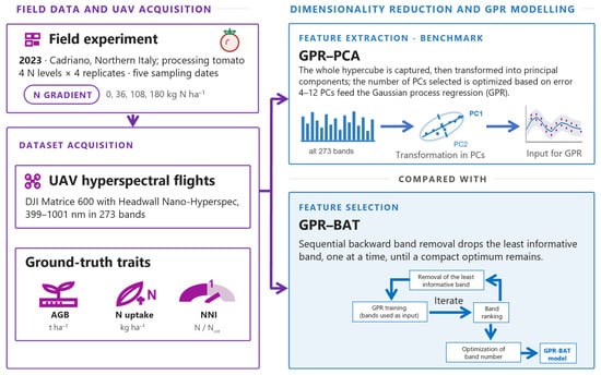
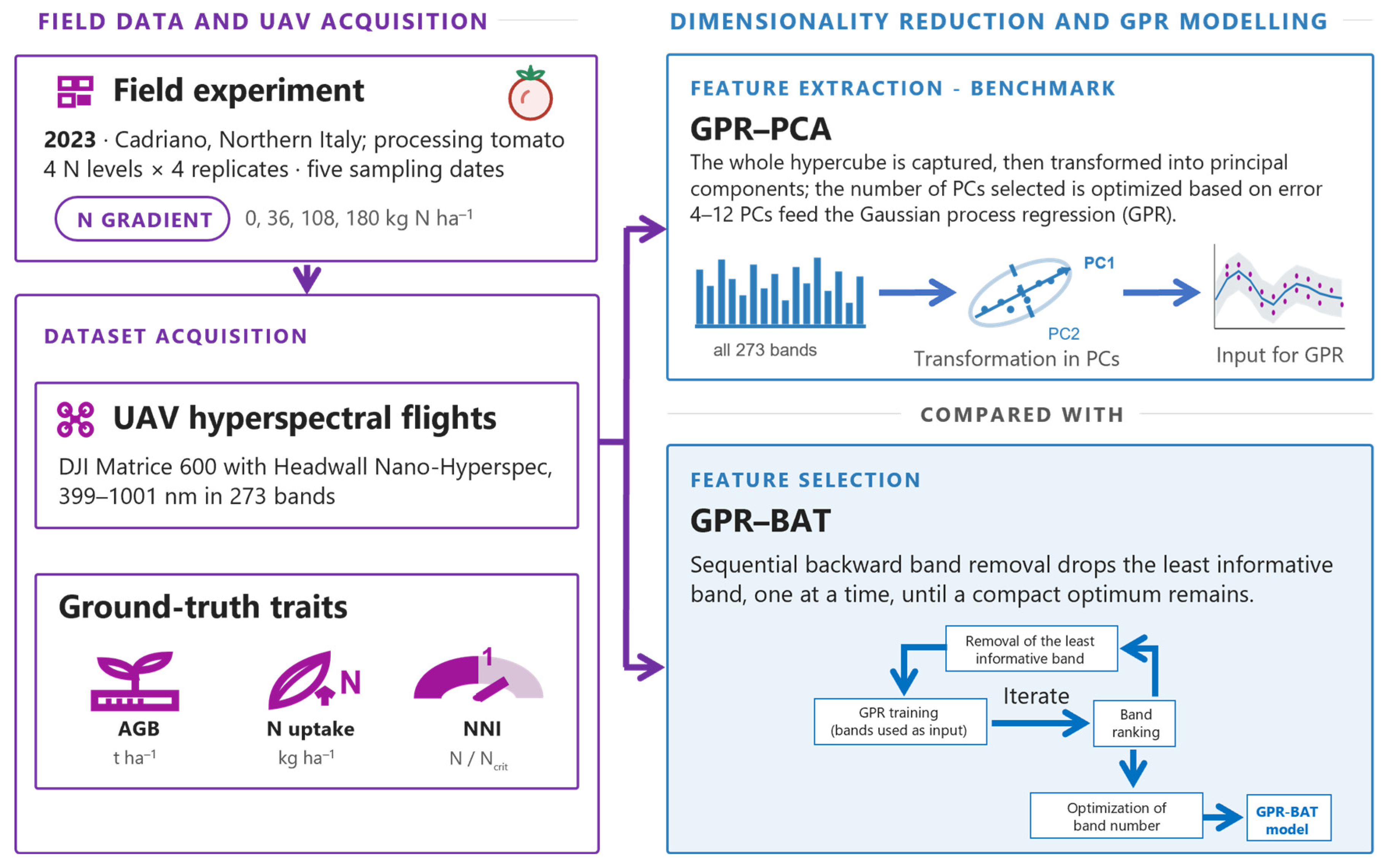
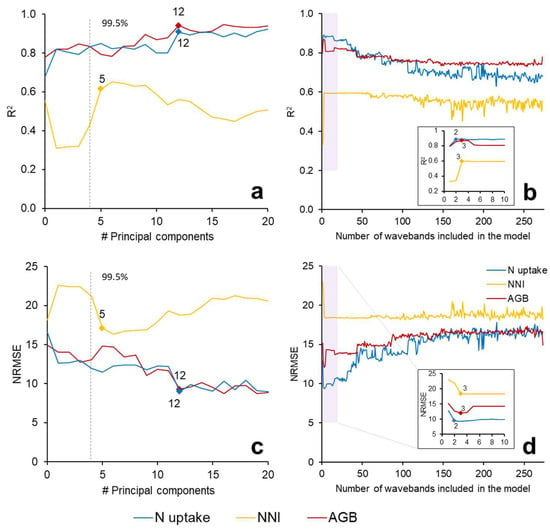
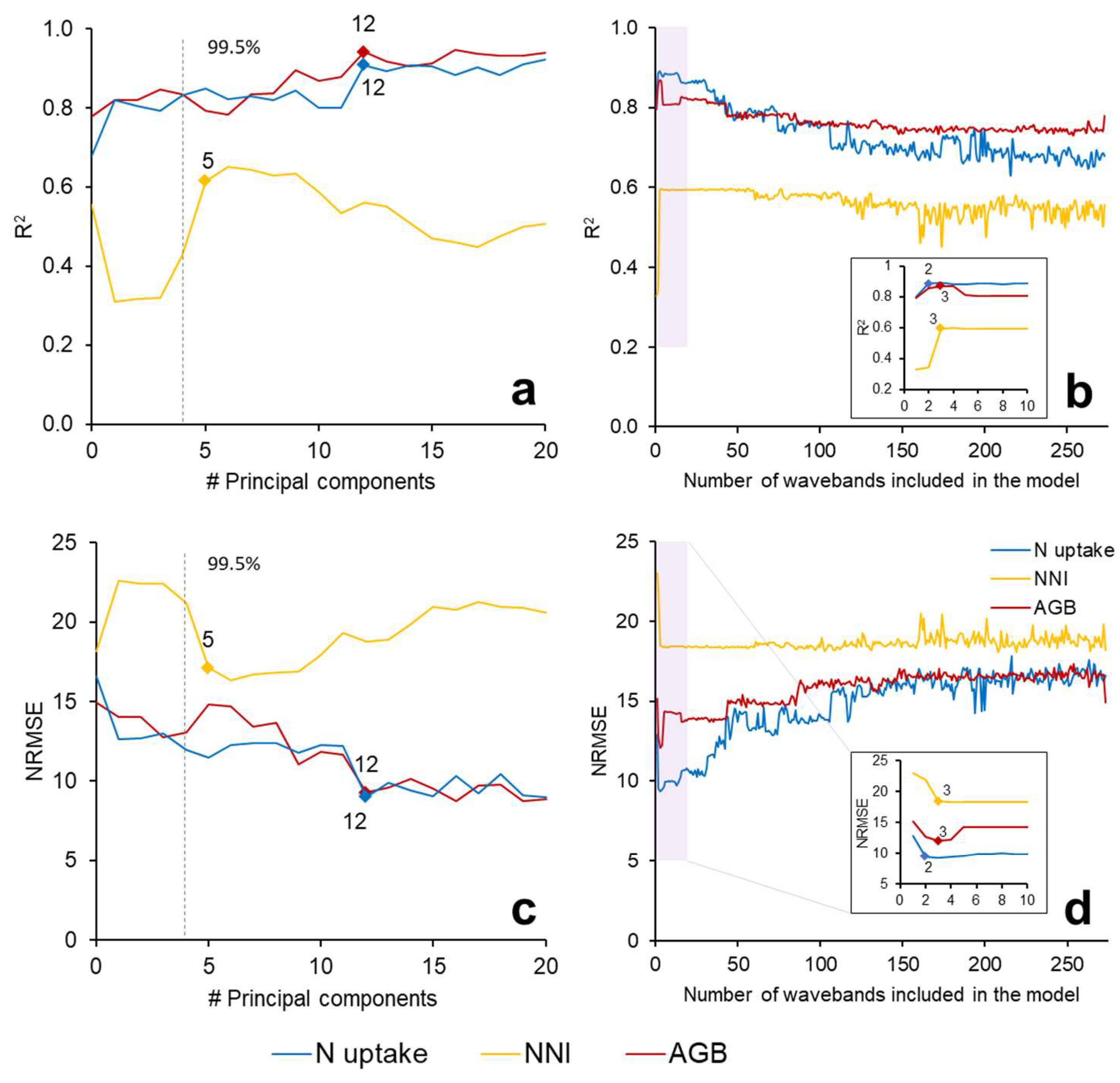
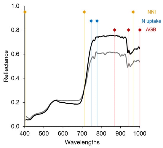
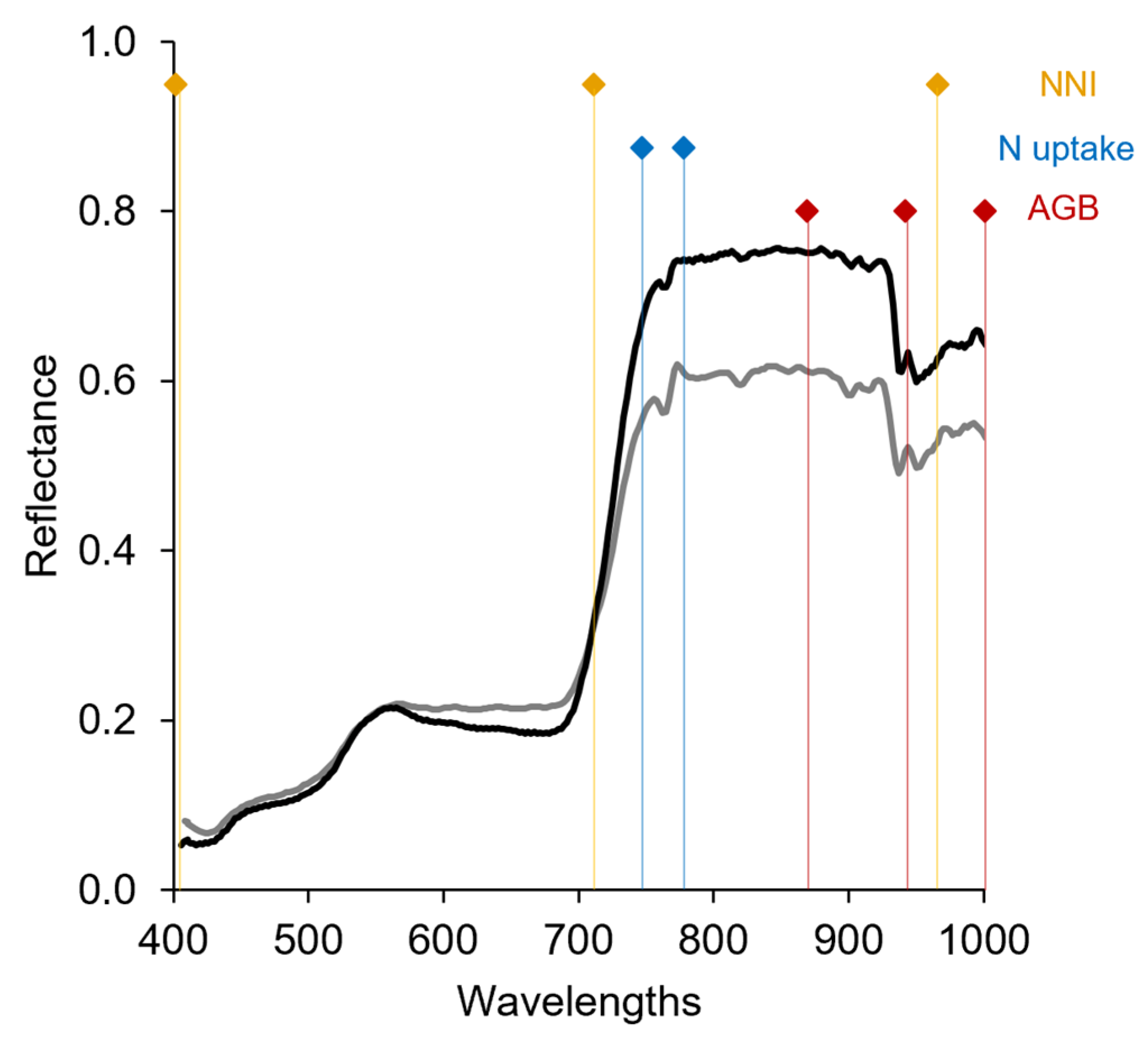
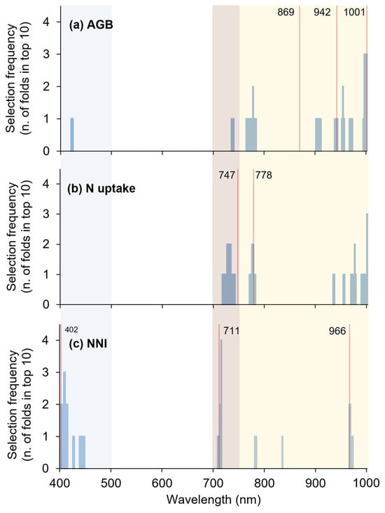
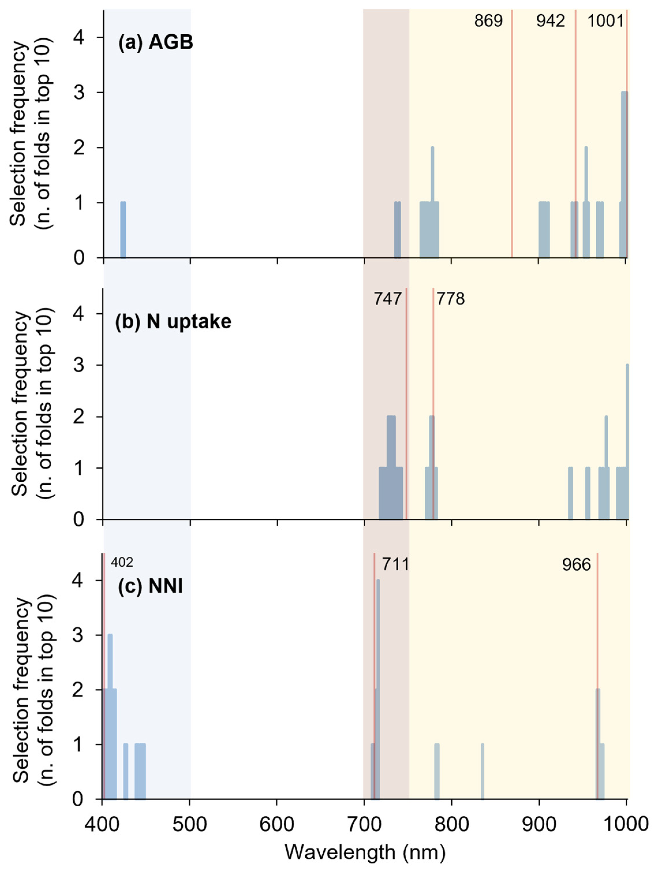
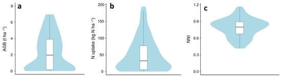
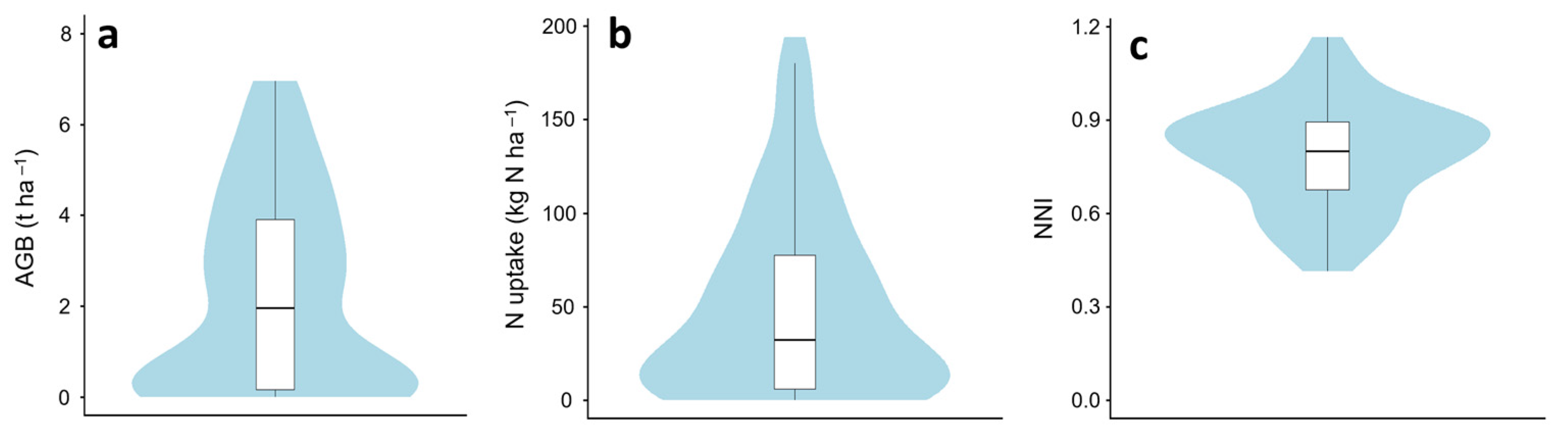
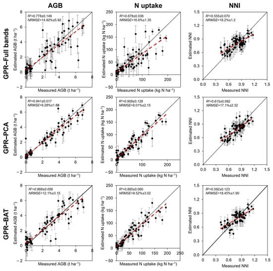
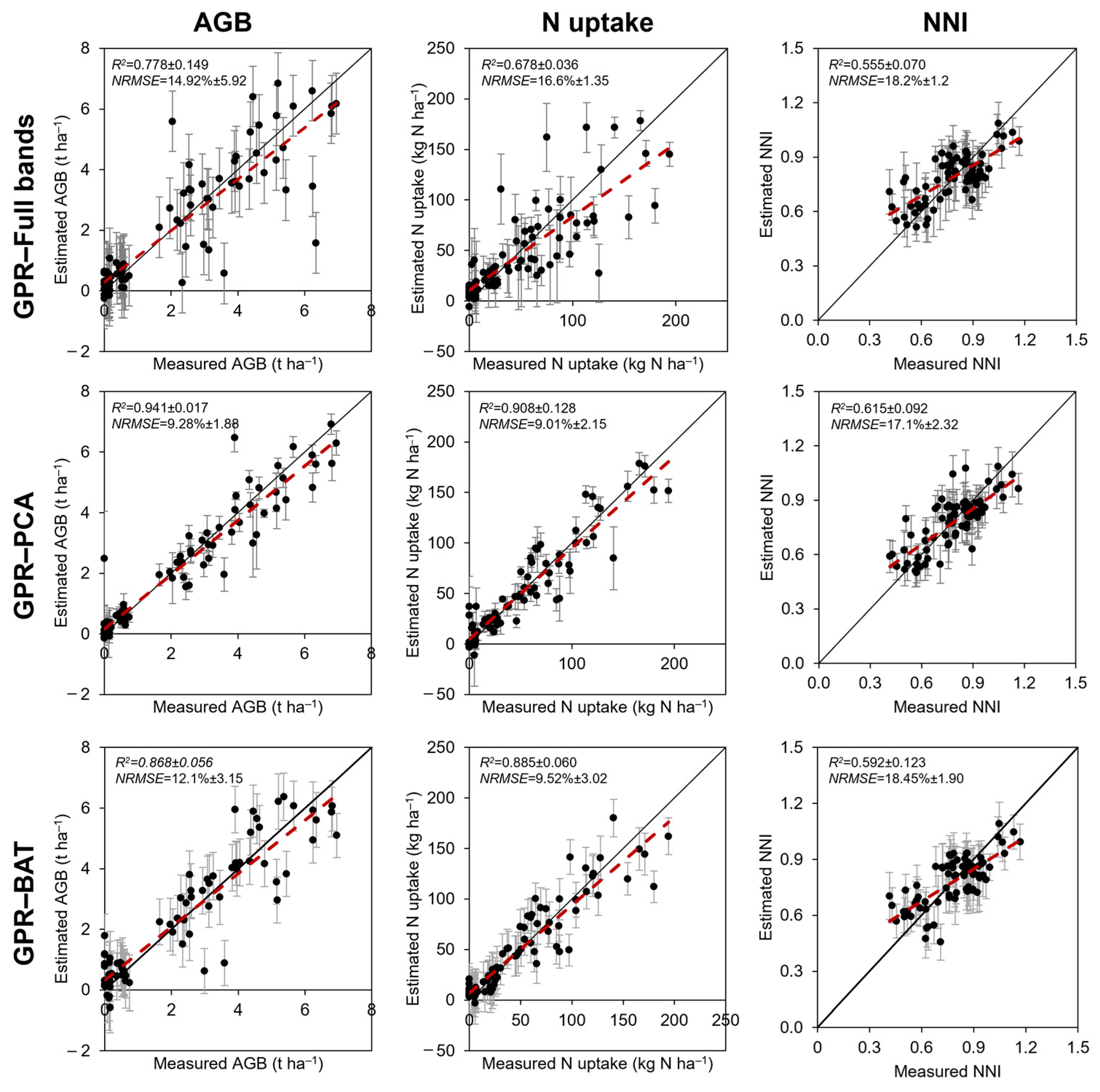
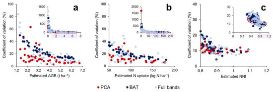

Disclaimer/Publisher’s Note: The statements, opinions and data contained in all publications are solely those of the individual author(s) and contributor(s) and not of MDPI and/or the editor(s). MDPI and/or the editor(s) disclaim responsibility for any injury to people or property resulting from any ideas, methods, instructions or products referred to in the content. |
© 2026 by the authors. Licensee MDPI, Basel, Switzerland. This article is an open access article distributed under the terms and conditions of the Creative Commons Attribution (CC BY) license.