Solutions of the Newtonian Plane Couette Flow with Dynamic Wall Slip Using Machine Learning Methods

Abstract

This study presents a comparative investigation of Physics-Informed Neural Networks (PINNs) and data-driven Deep Operator Networks (DeepONets) for predicting the evolution of plane Newtonian Couette flow with dynamic wall slip. First, a PINN framework is employed to solve flow for selected physical parameters. Subsequently, we develop a data-driven DeepONet, trained on high-fidelity numerical data, to learn the continuous solution operator across a broad range of slip boundary conditions and upper wall velocities. PINN achieves a relative $L_2$ error of 0.083% for the specific case considered. On the other hand, DeepONet shows a mean relative error of 0.340% on the standard test set and performs well when tested with a deterministic harmonic forcing outside the GRF-based forcing distribution used for training. While PINN gives accuracy for a specific configuration, the trained DeepONet can be reused for different boundary forcings and slip parameters without needing to be retrained. The compatibility of physics-based and data-driven models is highlighted. The results also demonstrate that DeepONet is a very effective surrogate model for quick parametric studies and the real-time prediction of fluid dynamics.

1. Introduction

This work concerns the use of Physics-Informed Neural Networks (PINNs) and data-driven Deep Operator Networks (DeepONets) for solving a one-dimensional flow problem with time-dependent boundary conditions, i.e., the plane Newtonian Couette flow with dynamic wall slip.

Although classical numerical methods, such as finite difference, finite element, and Crank–Nicolson schemes, can deliver accurate and stable solutions for such problems, their computational cost increases significantly when repeated simulations are required. This limitation becomes especially pronounced in parametric studies, uncertainty quantification, optimization, and real-time flow control, where the governing equations must be solved repeatedly for varying boundary conditions and material parameters. The challenge is further exacerbated when the wall motion is time-dependent and when slip takes place, introducing additional parameters, such as the slip coefficient and the slip relaxation parameter [1,2].

In recent years, scientific machine learning (SciML) has shown great potential as an alternative approach for solving problems of CFD. This method uses data and physics for modeling, prediction, and control of complex flow systems [3,4]. By learning representations of the underlying flow dynamics, neural network models can provide rapid predictions once trained, often at a lower computational cost than that of repeatedly solving the governing equations with conventional numerical methods. Consequently, machine learning has attracted increasing attention in fluid mechanics for applications, such as flow modeling and prediction, turbulence modeling, flow-field representation, optimization, active flow control, and surrogate modeling for repeated evaluations [5,6,7,8].

Among SciML approaches, PINNs have attracted considerable attention as a mesh-free method of solving partial differential equations (PDEs) [9]. PINNs are a class of neural networks incorporating physics laws into the training procedure of the neural networks, which are formulated in the form of PDEs or other governing equations. Unlike traditional neural networks that depend only on datasets, PINNs include these physics principles as constraints in the loss functions such that the solutions satisfy not only the dataset but also physics laws, including conservations law, boundary conditions, and/or dynamic equations. This approach allows PINNs to achieve high-precision predictions of unknown physical quantities using little or even no data and are therefore suitable for solving forward and inverse problems in the fields of science and engineering in the absence of mesh or labeled datasets [10,11,12]. The major shortcoming of PINNs, however, is their inability to generalize to different parameters: each new boundary condition or parameter set typically requires retraining or fine-tuning, which limits their scalability for real-time or multi-query applications.

To address this limitation, recent research has been paying increasing attention to the neural operator learning that attempts to approximate mappings between infinite-dimensional function spaces instead of pointwise solutions. Neural operators are specifically designed to approximate solution operators of PDEs, making them well suited for fluid dynamics problems where both inputs and outputs are continuous fields rather than finite-dimensional vectors [13,14,15]. Within this class of models, DeepONets [14,16] provide a theoretically grounded framework for learning nonlinear operators. DeepONets exhibit discretization invariance and strong generalization capabilities, making them particularly well suited for parametric PDEs with variable boundary and initial conditions.

Further advances have incorporated physical constraints into operator learning frameworks, resulting in physics-informed DeepONets. The latter benefit from combining the flexibility of operator learning with the robustness and physical consistency of physics-informed learning, greatly lowering data needs as well as boosting extrapolation abilities [17,18,19]. Recent studies have demonstrated the effectiveness of such models for heat conduction [18], advection–diffusion–reaction systems [20], and other parametric PDEs under complex and time-dependent boundary conditions, achieving orders of magnitude speedups compared with classical numerical solvers.

Motivated by these developments, the present work investigates the Newtonian plane Couette flow with linear dynamic wall slip, a problem that introduces both time-dependent boundary forcing and parametric slip behavior.

The classical no-slip assumption that fluid particles stick to solid boundaries has been conveniently employed in theoretical and computational fluid mechanics. However, it is well established that the no-slip condition is violated in many flows of industrial interest, as well as in viscometric flows, and in microfluidic applications [1,21,22], and may be exhibited not only by complex fluids but also by Newtonian ones [23]. It is well documented that wall slip may affect the stability of polymer melt extrusion, enhancing or, in certain cases, suppressing instability [21,22]. It may also lead to inaccurate rheological parameter estimates in viscometric flows [24] and is routinely exhibited by Newtonian fluids in micro- and nano-fluidic devices [23]. The various proposed mechanisms of wall slip and the different phenomenological models are discussed in the reviews of Hatzikiriakos [1,25] and Malkin and Patlazhan [22].

Navier [26] was the first to propose a linear slip law expressing the slip velocity, i.e., the relative velocity of the adjacent fluid particles to that of the wall (which may be moving), $v_s$, as a function of the (local) wall shear stress, ${\mathsf{\tau }}_s$,

$$v_s={\displaystyle \frac{1}{\beta }}{\mathsf{\tau }}_s$$

(1)

where $\beta$ is the slip coefficient. This varies with the temperature and the pressure [21,22] and depends on the fluid properties (e.g., molecular weight and distribution) and the properties of the wall–fluid interface. When $\beta \to \infty$, the standard no-slip condition is obtained ($v_s=0$). Nonlinear extensions of the Navier slip law (1), e.g., the power-law slip model, have been proposed [1,22]. Equation (1) and these extensions are static, i.e., they work well at steady state but fail to capture any memory effects, such as transient overshoots and slip velocity relaxation. Pearson and Petrie [27] generalized Equation (1) by adding a time-derivative term with a slip relaxation parameter, $\mathsf{\lambda }$, resulting in a ‘retarded’ slip law,

$$v_s+\lambda {\displaystyle \frac{\partial v_s}{\partial t}}={\displaystyle \frac{1}{\beta }}{\mathsf{\tau }}_s$$

(2)

where $t$ is the time. Equation (2) reduces to the static Navier-slip law (1) when $\lambda =0$ or in steady-state flow. As $\lambda$ increases, memory effects become significant and the evolution of the slip velocity lags variations in wall shear stress. Memory effects have been observed in experiments on molten polymer [28,29]. Dynamic wall slip has also been reported in the molecular dynamic simulations of Thalakkottor and Mohseni [30] for both gas and simple liquid flows near oscillating walls. Kazatchkov and Hatzikirakos [31] and Malkin and Patlazhan [22] pointed out that retarded wall slip becomes relevant at high shear rates. Since reaching a steady state in the presence of dynamic wall slip may take very long times, special attention is required to obtain reliable estimates of the rheological parameters in transient rheometric experiments.

The implications of dynamic wall slip have been demonstrated in various recent analytical and numerical studies on transient one- and two-dimensional Newtonian Couette and Poiseuille flows [32,33,34]. The central result, in all flow configurations, is that wall slip generally damps the flow development and this damping is enhanced as the slip relaxation parameter is increased, in good agreement with experimental observations [28,29]. In particular, the plane Couette flow is a prototype viscometric flow, but it is also widely used to study viscous shear-driven flow dynamics and wall–fluid interactions [35]. Its simplicity allows rigorous theoretical analysis while capturing essential physical mechanisms relevant to rheological and microfluidic applications.

These characteristics also make the problem a suitable setting for examining different SciML approaches under time-dependent boundary forcing and dynamic wall slip. Although the PINN is well suited to solve individual configurations accurately, each new boundary condition or parameter set generally requires retraining. The main objective here is not to replace conventional numerical methods for a single one-dimensional flow problem, but to examine the advantages of operator learning when repeated solutions are required for varying boundary forcing and slip parameters. Accordingly, this study compares an instance-specific PINN formulation with a data-driven DeepONet for the prediction of the velocity field.

Specifically, a PINN is employed to solve a representative moderate slip case, while a Balanced DeepONet is trained to learn the solution operator across a wide range of slip coefficients, slip relaxation parameters, and upper wall velocity functions. It should be noted that the above comparison highlights the basic trade-off between physics-guided optimization and operator learning approaches that enable rapid generalized predictions across different settings.

By addressing dynamic boundary motion and slip relaxation within an operator learning framework, this work extends the applicability of DeepONets to unsteady viscous flows with complex wall dynamics. The results have shown how neural operator models can be used as efficient surrogate models for repeated parametric flow evaluations, while also providing insights into the complementary roles of PINNs and DeepONets in scientific machine learning for fluid mechanics.

The rest of this paper is organized as follows: Section 2 provides theoretical foundations, recalling the main equations governing the Newtonian plane Couette flow with dynamic wall slip, along with the PINN and DeepONet formulations for parametric boundary conditions. Section 3 presents the results and discussion, beginning with the application of the PINN model to specific Couette flow cases. This is followed by an evaluation of the data-driven DeepONet framework, i.e., its ability to map varying boundary forcing functions and slip parameters to spatio-temporal velocity fields. Subsequently, a comparative analysis of the two frameworks in terms of accuracy and efficiency is performed. Finally, Section 4 summarizes the key findings of this study and discusses some ideas for future work.

2. Formulations

2.1. The Newtonian Plane Couette Flow with Dynamic Wall Slip

The physical problem considered is the time-dependent, incompressible Newtonian plane Couette flow between two infinite parallel plates separated by a distance $d$. Initially, at $t=0$, the fluid is at rest everywhere. At time $t>0$, the upper plate ($y=d$) moves in the $x$-direction with a given velocity $V_{0}f\left(t\right)$, while the lower plate ($y=0$) remains fixed. For a Newtonian fluid with constant density $\rho$ and dynamic viscosity $\mu$, the $x$-momentum equation reduces to the one-dimensional diffusion equation:

$$\rho {\displaystyle \frac{\partial v}{\partial t}}=\mu {\displaystyle \frac{{\partial }^{2}v}{\partial y^2}}, t\ge 0, 0\le y\le d$$

(3)

Dynamic wall slip following Equation (2) is assumed to occur only along the fixed plate, whereas the classical no-slip condition applies at the moving plate. Thus, the boundary conditions for the velocity $v(y,t)$ read:

$$v\left(0,t\right)+\lambda {\displaystyle \frac{\partial v}{\partial t}}\left(0,t\right)={\displaystyle \frac{\mu }{\beta }}{\displaystyle \frac{\partial v}{\partial y}}\left(0,t\right), t>0$$

(4)

At the fixed lower plate, a linear dynamic slip law is employed, which generalizes the classical Navier slip condition by incorporating a relaxation term. This dynamic slip law accounts for the time-dependent response of the fluid–wall interface and takes the form [35]:

$$v(d,t)=V_{0}f\left(t\right),t>0$$

(5)

Since the fluid is initially at rest, the initial condition is

$$v\left(y,0\right)=0, 0\le y\le d$$

(6)

To nondimensionalize the problem of Equations (3)–(6), we scale lengths by $d$, time by the diffusion time scale $d^2\rho /\mu$, and the velocity by the characteristic velocity $V_0$ of the moving plate. For simplicity, we retain the same symbols for the dimensionless variables. The dimensionless form of the initial boundary value problem becomes:

$${\displaystyle \frac{\partial v}{\partial t}}={\displaystyle \frac{{\partial }^{2}v}{\partial y^2}}, t>0, 0\le y\le 1$$

(7)

subject to the boundary conditions:

$$v\left(0,t\right)+{\Lambda }_s{\displaystyle \frac{\partial v}{\partial t}}\left(0,t\right)={\displaystyle \frac{1}{B}}{\displaystyle \frac{\partial v}{\partial y}}\left(0,t\right), t>0$$

(8)

$$v\left(1,t\right)=f\left(t\right), t>0$$

(9)

and the initial condition:

$$v\left(y,0\right)=0, 0\le y\le 1$$

(10)

Two dimensionless parameters emerge from the nondimensionalization process: the slip number,

$$B\equiv {\displaystyle \frac{\beta d}{\mu }}$$

(11)

and the slip relaxation number

$${\Lambda }_s\equiv {\displaystyle \frac{\lambda \mu }{\rho d^2}}$$

(12)

The slip number $B$ quantifies the ease of slip at the interface, with larger values indicating weaker slip (approaching no-slip as $B\to \mathrm{\infty }$) and smaller values indicating stronger slip. The dimensionless slip relaxation number ${\Lambda }_s$ characterizes the temporal memory effect of the dynamic slip law, representing the ratio of the slip relaxation time scale to the diffusion time scale. When ${\Lambda }_s=0$, the static Navier slip condition is recovered [1].

The initial boundary value problem described by Equations (7)–(10) was solved by Abou Hasan et al. [35] using an efficient numerical method based on weighted average finite differences (WAFD). Their study considered three distinct cases of motion for the moving plate at $y=1$: constant speed, oscillatory speed, and single-period sinusoidal speed. The WAFD scheme with a weighting factor $\theta =0.5$ corresponds to the well-known Crank–Nicolson (CN) implicit scheme. In the present work, we adopt this method to generate numerical reference solutions for both training and evaluation purposes.

2.2. Physics-Informed Neural Network (PINN)

Initially, the Newtonian plane Couette flow with linear dynamic wall slip is solved for the special case of ${\Lambda }_s=0.5,$ $B=1$ (moderate slip) and $f\left(t\right)=\sin \left(4\pi t\right)$ (sinusoidal upper speed) using the Physics-Informed Neural Network (PINN) framework [9].

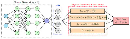
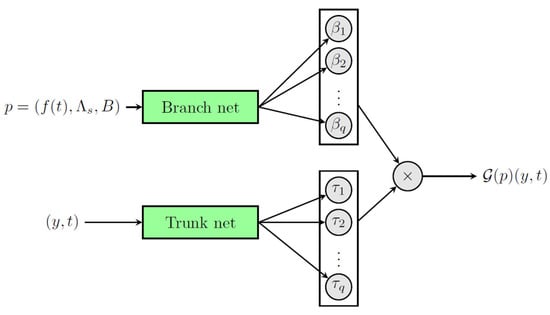
The unknown velocity field $v\left(y,t\right)$ is approximated by a fully connected feed-forward neural network $v_{\theta }(y,t)$, parameterized by $\theta$. In this case, $\theta$ represents all trainable parameters, which include the weights and bias terms optimized during training. The network takes the spatial and temporal coordinates $\left(y,t\right)$ as inputs and outputs the predicted velocity (Figure 1). Multiple hidden layers with nonlinear activation functions (e.g., hyperbolic tangent) are employed to ensure sufficient representational capacity for smooth solutions of parabolic differential equation. Spatial and temporal derivatives required by the governing equation and boundary conditions are computed via automatic differentiation (AD), which provides machine precision accuracy and avoids numerical discretization errors.

Figure 1. Schematic of the Physics-Informed Neural Network (PINN) architecture used to approximate the velocity field $v(y,t)$.

The PINN model is trained by minimizing a composite loss function defined as [9]

$$\mathcal{L}=w_{pde}{\mathcal{L}}_{pde}+w_{bc0}{\mathcal{L}}_{bc0}+w_{bc1}{\mathcal{L}}_{bc1}+{w_{ic}\mathcal{L}}_{ic},$$

(13)

where each term ${\mathcal{L}}_i$ enforces a specific physical constraint with a corresponding weight $w_i$.

The residual of the governing equation is given by

$${\mathcal{L}}_{pde}={\displaystyle \frac{1}{N_{pde}}}{\displaystyle \sum _{i=1}^{N_{pde}}}{\left({\displaystyle \frac{\partial v_{\theta }}{\partial t}}(y_i,t_i)-{\displaystyle \frac{{\partial }^2{v}_{\theta }}{\partial y^2}}(y_i,t_i)\right)}^2$$

(14)

evaluated at $N_{pde}$ collocation points randomly sampled within the spatio-temporal domain.

The initial condition loss, defined as

$${\mathcal{L}}_{ic}={\displaystyle \frac{1}{N_{ic}}}{\displaystyle \sum _{i=1}^{N_{ic}}}{\left(v_{\theta }(y_i,0)\right)}^2$$

(15)

quantifies the residuals of the initial condition on $N_{ic}$ points. The boundary condition loss consists of two parts:

$${\mathcal{L}}_{bc0}={\displaystyle \frac{1}{N_{bc}}}{\displaystyle \sum _{i=1}^{N_{bc}}}{\left[v_{\theta }\left(0,t_i\right)+{\Lambda }_s{\displaystyle \frac{\partial v_{\theta }}{\partial t}}\left(0,t_i\right)-{\displaystyle \frac{1}{B}}{\displaystyle \frac{\partial v_{\theta }}{\partial y}}\left(0,t_i\right)\right]}^2$$

(16)

and

$${\mathcal{L}}_{bc1}={\displaystyle \frac{1}{N_{bc}}}{\displaystyle \sum _{i=1}^{N_{bc}}}{\left[v_{\theta }\left(1,t_i\right)-\sin \left(4\pi t_i\right)\right]}^2,$$

(17)

where $N_{bc}$ is the total number of sampled points in time. Notice that all loss terms are a function of the network weight and bias parameters, denoted by $\theta =(w_i,b_i)$. These parameters are optimized using gradient-based optimization algorithms. An adaptive optimizer (Adam) [36] is employed first to achieve rapid convergence, followed by a quasi-Newton method (L-BFGS) [37] to further reduce the loss and improve solution accuracy.

The PINN methodology offers a flexible and robust framework for solving time-dependent flow problems with non-standard boundary conditions, such as linear dynamic wall slip. The resulting model provides a continuous, differentiable approximation of the velocity field over the entire space–time domain, making it well suited for parametric studies and further theoretical analysis.

2.3. Deep Operator Network (DeepONet) Formulation for Parametric Boundary Conditions

The DeepONet framework, first introduced by Lu et al. [16], offers an excellent way to learn nonlinear operators mapping between the infinite-dimensional function spaces. This research further explores the DeepONet architecture to solve the problem of the parametric plane Couette flow as explained in Section 2.1. In contrast with the traditional PINNs solving the PDE for a given set of input parameters, the DeepONet learns the mapping of the inputs (including functions and scalars) to the output (velocity field solution). This method has significant advantages when applied to the current case study because the solution depends on the time-varying upper plate velocity function $f\left(t\right)$ and two dimensionless numbers, $B$ and ${\Lambda }_s$.

We define the parameter space $\mathcal{P}$ consisting of elements $p=(f,{\Lambda }_s,B)$, where $f\in \mathcal{F}$ is a function in an infinite-dimensional function space representing the upper plate velocity and ${\Lambda }_s$, $B$ are positive scalar parameters. For every possible parameter combination in the set $\mathcal{P}$, there exists a unique solution $v=v\left(p\right)(y,t)$ of the initial boundary value problem defined by Equations (7)–(10). Consequently, we can define the solution operator $\mathcal{G}:\mathcal{P}\to \mathcal{S}$, where $\mathcal{S}$ is the solution space of velocity fields, such that

$$\mathcal{G}\left(p\right)(y,t)=v\left(p\right)(y,t)$$

(18)

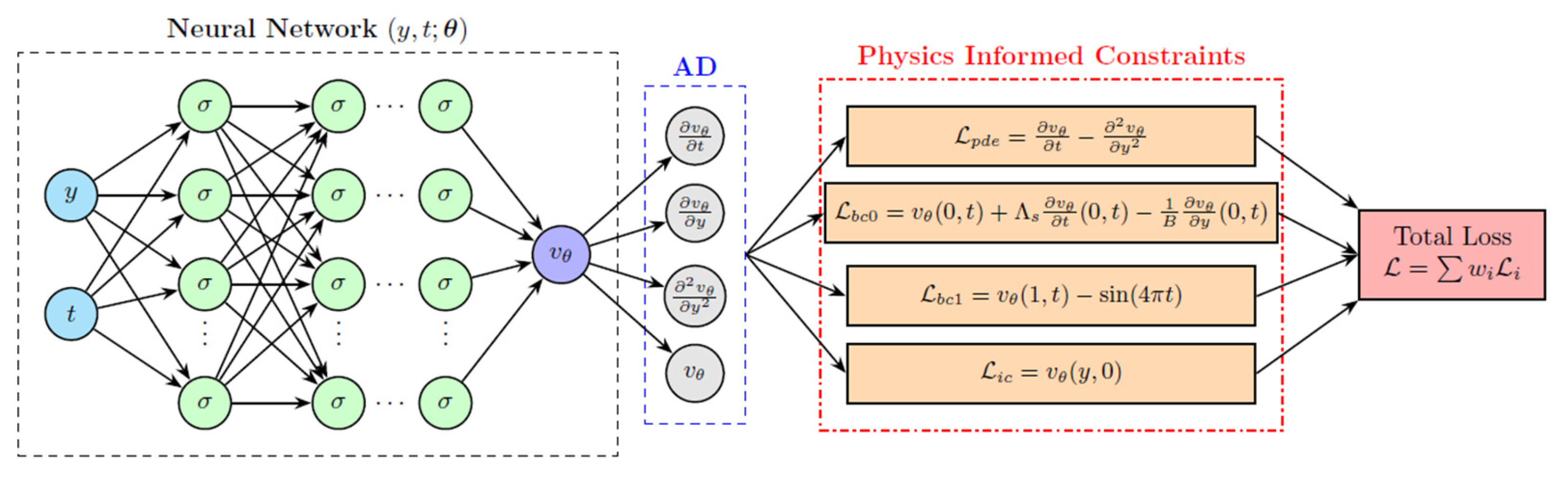
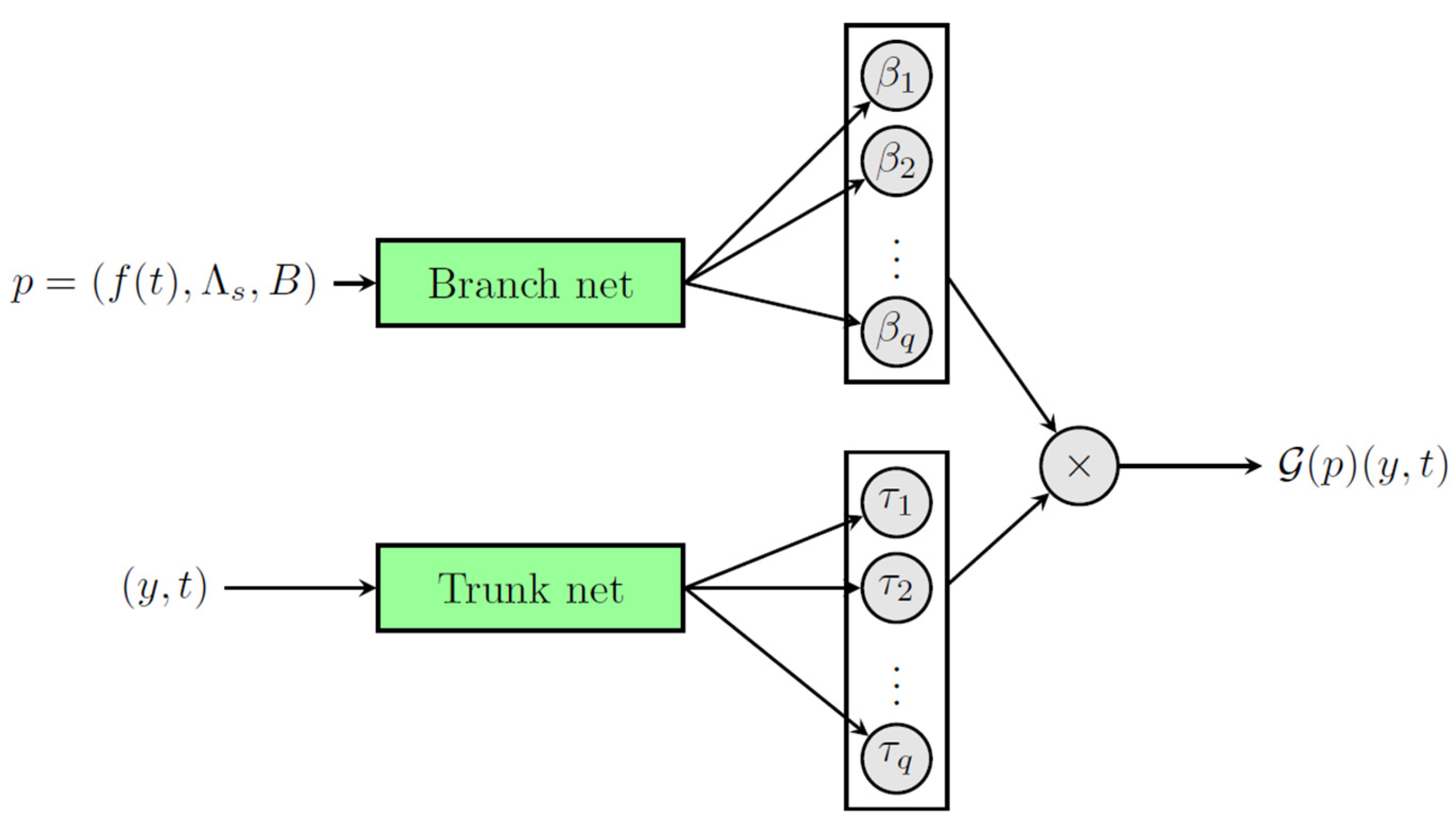
The DeepONet architecture is intended to approximate the operator $\mathcal{G}$ by taking the parameter configuration $p$ and the space–time coordinates $(y,t)$ as input and giving the output as the predicted velocity $\widehat{v}(y,t)$. The architecture, illustrated in Figure 2, comprises two main sub-networks: a branch network and a trunk network.

Figure 2. Schematic representation of the Deep Operator Network (DeepONet) architecture.

The role of the branch network is to process all parameters of the input describing the problem at a particular instance. In our formulation, these include:

^1. 

The function input $f\left(t\right)$: In practice, the continuous function $f\left(t\right)$ is represented by its values at $m$ discrete sensor points in the time domain, denoted as $\left[f\left(t_1\right),f\left(t_2\right),...,f\left(t_m\right)\right]$. These sensor points are typically chosen to cover the time interval of interest $\left[0,T\right]$.

^2. 

The scalar parameters: The slip relaxation number ${\Lambda }_s$ and the slip number $B$ are appended to the discretized function values, forming a composite input vector of dimension $m+2$:

$$\mathrm{Branch} \mathrm{input}=\left[f\right(t_1),f(t_2),...,f(t_m),{\Lambda }_s,B]$$

The branch network, being a fully connected feed-forward neural network, gets this input and outputs a latent representation vector, $\left[{\beta }_1, {\beta }_2,\dots , {\beta }_q\right]$, of dimension $q$ [16]. This vector can be interpreted as the coefficients for a set of learned basis functions that encode the influence of the input parameters on the solution.

The trunk network takes as input the spatio-temporal coordinates $\left(y,t\right)$ at which the solution is evaluated. For the plane Couette flow problem, $y\in \left[\mathrm{0,1}\right]$ is the dimensionless distance from the fixed lower plate, and $t\in [0,T]$ is the dimensionless time. The trunk network is also a fully connected neural network that generates a $q$-dimensional vector $\left[{\tau }_1, {\tau }_2,\dots , {\tau }_q\right]$, which can be interpreted as a set of $q$ basis functions evaluated at $\left(y,t\right)$.

The final output of the DeepONet is the dot product of the branch and trunk network outputs, optionally with an added bias term:

$$\widehat{\mathcal{G}}\left(p\right)\left(y,t\right)={\displaystyle \sum _{k=1}^q}{\beta }_k\left(p\right)\cdot {\tau }_k\left(y,t\right)+b_0,$$

(19)

where $b_0$ is a trainable bias parameter. This is an elegant way to let the network approximate the solution using a linear combination of nonlinear functions (the basis, learned by the trunk network), where the coefficients are nonlinear functions of the parameters (learned by the branch network).

It should be noted that the unstacked DeepONet architecture employed here (see Figure 1), which consists of distinct branch and trunk networks and their outputs combined via dot product, has been demonstrated by Lu et al. [16] to have better performance than stacked models with lower computational cost.

The DeepONet framework possesses a clear advantage over conventional numerical solvers and standard PINNs for this problem. In fact, once trained on a sufficiently representative set of parameter values, it can very quickly evaluate the velocity field $v\left(y,t\right)$ for any new combination of the upper plate velocity function $f\left(t\right)$, the slip relaxation number ${\Lambda }_s$, and the slip number $B$ within the parameter ranges considered in this study. These predictions are obtained without retraining the model or re-solving the governing equations. Thus, DeepONet enables one to efficiently use the model as a surrogate in many-query calculations, such as uncertainty quantification, sensitivity analysis, and real-time control.

2.4. Verification of the Numerical Reference Solution

The Crank–Nicolson solution employed for dataset generation and model evaluation was verified through grid- and time-step refinement for the representative case $B=1$, ${\Lambda }_s=0.5$, and $f\left(t\right)=\mathrm{s}\mathrm{i}\mathrm{n}\left(4\pi t\right)$. Spatial refinement from 100 to 200 and subsequently to 400 grid points reduced the relative difference between successive solutions from $2.23\times {10}^{-4}$ to $1.10\times {10}^{-4}$. Temporal refinement over the corresponding resolutions reduced the successive relative difference from $8.87\times {10}^{-4}$ to $2.52\times {10}^{-4}$, with an observed temporal convergence rate of approximately 1.8. Most importantly, the relative $L_2$ difference between the $200\times 200$ resolution used for the numerical dataset and that for $400\times 400$ one was only $2.73\times {10}^{-4}$(0.0273%). These results confirm that the adopted discretization provides a sufficiently resolved numerical reference for evaluating the machine learning predictions.

3. Results and Discussion

3.1. PINN

In this section, we use the PINN model described in Section 2.1 for solving the specific case of the Newtonian plane Couette flow (e.g., $B=1,$ ${\Lambda }_s=0.5,$ $f\left(t\right)=\sin \left(4\pi t\right)$). In order to get the velocity field $v(y,t)$, a neural network with four hidden layers, each consisting of $90$ neurons, was employed. The hyperbolic tangent activation function was applied to all layers. The training of the PINN model was conducted using random points from the space–time domain $\left[\mathrm{0,1}]\times [\mathrm{0,1}\right]$. In particular, $N_{pde}={10}^4$ interior points were used to enforce the PDE residual, while $N_{ic}=3000$ and $N_{bc}=3000$ points were used to impose the initial and boundary conditions, respectively. The training process uses the MSE loss function (13), which considers all terms proportionally to their weights. The residuals of the differential equation and boundary condition at $y=0$ are weighted by $w_{pde}=w_{bc0}=1$, while the errors associated with the initial and boundary condition at $y=1$ are weighted by ${ w}_{ic}=w_{bc1}=10$. Different training configurations were tested, with the weights giving the best results. The optimization was carried out in two stages: first, the Adam optimizer was applied for $\mathrm{10,000}$ iterations at a learning rate of ${10}^{-4}$, and then L-BFGS optimization was performed for up to $4000$ iterations to refine the solution.

The accuracy of the model was evaluated using the relative $L_2$ error metric

$$Rel L_2={\displaystyle \frac{{\Vert {\mathit{v}}_{\mathit{p}\mathit{r}\mathit{e}\mathit{d}}-v_{ref}\Vert }_2}{{\Vert v_{ref}\Vert }_2}}$$

(20)

which measures the global discrepancy between the predicted velocity field ${\mathit{v}}_{\mathit{p}\mathit{r}\mathit{e}\mathit{d}}$ and the reference solution $v_{ref}$ obtained from the CN solver.

To determine the effect of stochastic initialization and sampling, the procedure was performed five times with different seeds. For each run, the training time was recorded and the relative $L_{2 }$ error was computed against the numerical reference solution (CN) on a uniform $200\times 200$ evaluation grid. The results corresponding to the mean and standard deviation across all runs are given in Table 1.

Table 1. Statistical performance of the proposed PINN architecture across five independent runs.

Metric	Mean Value	Standard Deviation	Best Achievement
Rel. ${\mathit{L}}_2$ Error (%)	$0.083$	$0.006$	$0.075$
Training Time (min)	$46.83$	$7.3$	$38.20$

The presented results have demonstrated consistent accuracy, with a mean relative $L_2$ error of $0.083\%$ and a small standard deviation of $0.006\%$, reflecting the consistency of the developed model. The best run achieved an error of $0.075\%.$ The average training time was $46.83$ minutes, with some variability across runs due to differences in optimization convergence. The results obtained confirm that the proposed PINN approach allows generating reliable and accurate solutions for the oscillatory Couette flow problem, while maintaining consistent performance across multiple independent training runs.

Throughout the subsequent analyses, the results and the visualizations presented below correspond to the representative models from the group that have achieved median test set performance, thus ensuring that the reported efficiency and accuracy are indicative of the typical model behavior rather than an outlier.

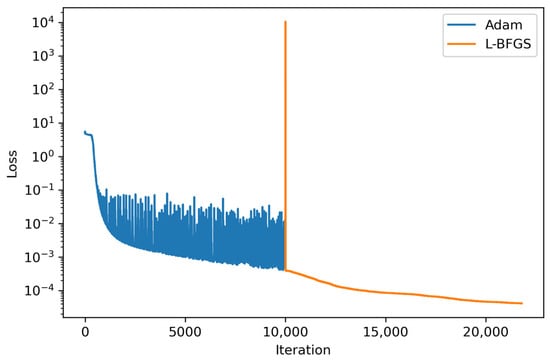
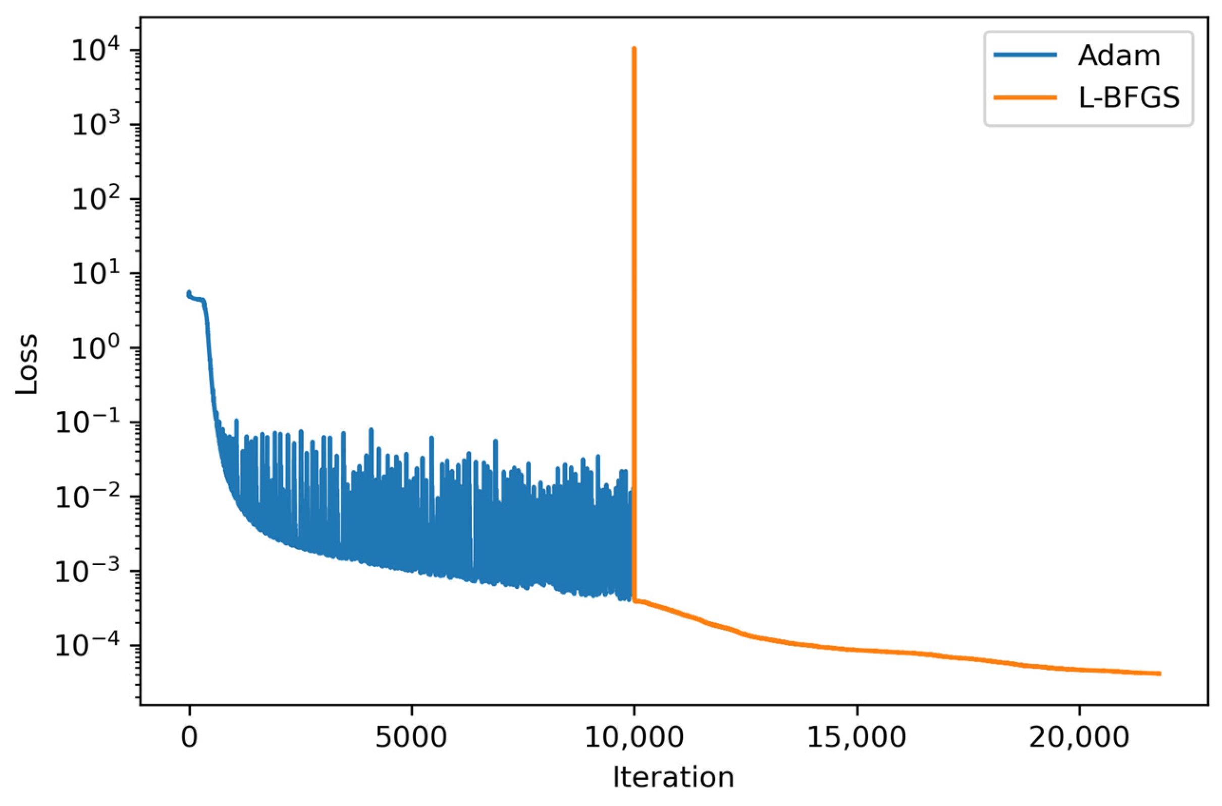
Figure 3 illustrates the training convergence of the proposed PINN model, which shows the two-stage optimization strategy mentioned above. In the initial Adam stage, there is a rapid drop of the loss function by several orders of magnitude within the first few thousands of iterations, meaning the efficient learning of the physics constraints at the first stage of the process. After approximately $\mathrm{10,000}$ iterations, the loss gradually stabilizes around ${10}^{-4}$, meaning that the optimizer converges to a plateau characteristic of first order optimization methods. At this point, the L-BFGS optimizer is applied to further minimize the residual loss. There is a noticeable rise in the loss at the moment of switching to the next optimizer, which is a common feature of changing the optimization procedure. Subsequently, L-BFGS provides significant improvement in convergence and reduces the loss by another order to get the value ${10}^{-5}$. This behavior is in agreement with previous results where the advantage of second order optimizers in achieving higher accuracy was shown for PINNs after the initial Adam training phase [38,39].

Figure 3. Training convergence of the PINN model showing the evolution of the total loss function.

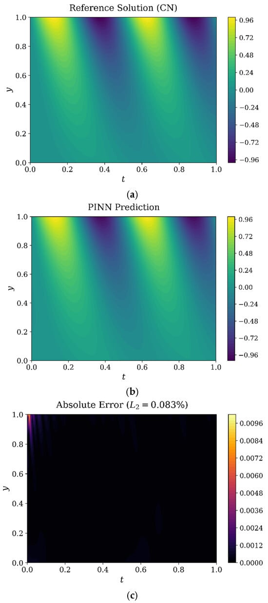
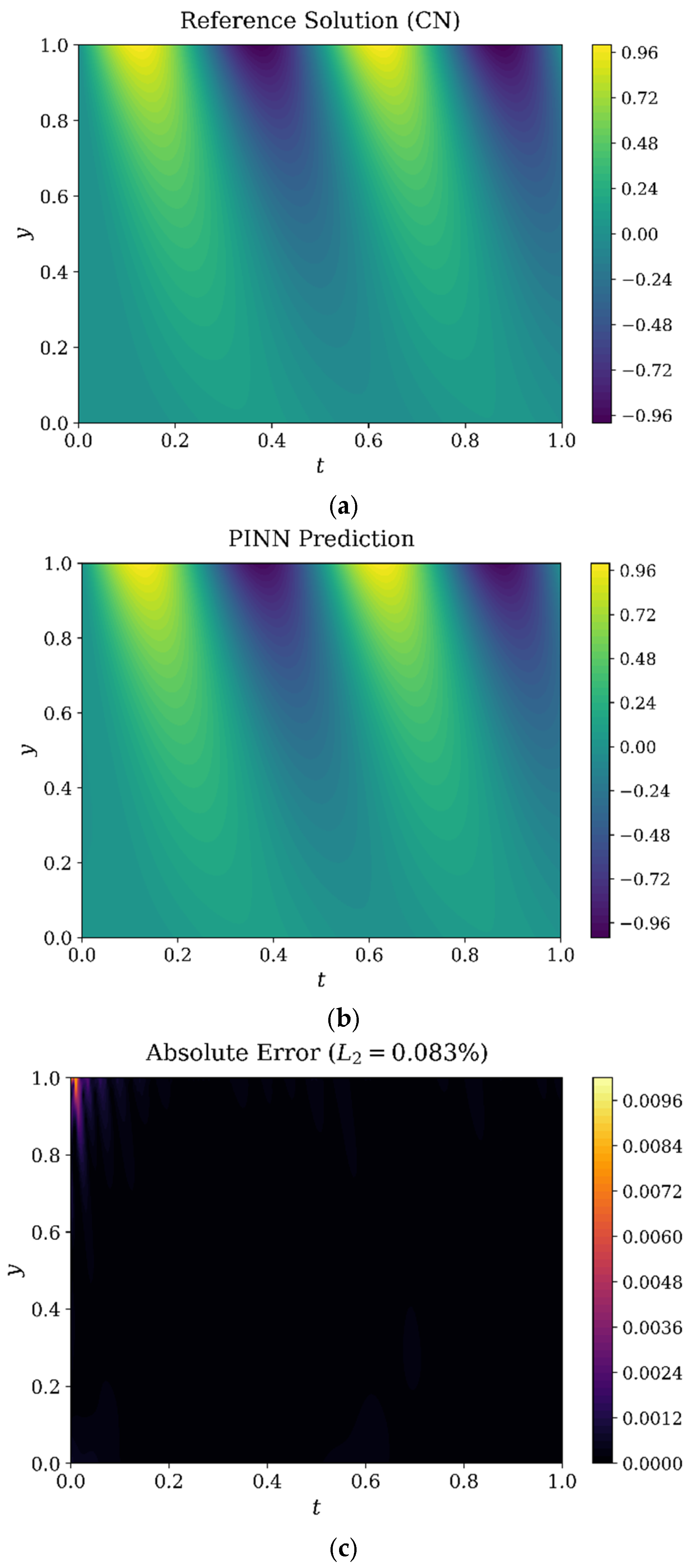
Figure 4 presents a comparison between the velocity field predicted by the proposed physics-informed neural network and the reference solution obtained using the CN numerical solver. The spatio-temporal evolution of the velocity field is shown over the entire computational domain $(y,t)\in \left[\mathrm{0,1}\right]\times \left[\mathrm{0,1}\right]$. As shown in the first two contour plots, the PINN prediction is in excellent agreement with the reference CN solution. The model accurately captures the characteristic oscillatory behavior induced by the time-dependent boundary condition imposed at the upper plate. In particular, the spatial decay of the oscillations from the upper boundary toward the lower wall is faithfully reproduced, demonstrating that the PINN successfully learns the underlying diffusion dynamics governing the system.

Figure 4. Results for oscillatory Couette flow with $B=1$, ${\Lambda }_s=0.5$ and $f\left(t\right)=\mathit{sin}\left(4\pi t\right)$: (a) numerical (CN) velocity; (b) PINN velocity prediction; (c) absolute $L_2$ error.

The absolute error depicted in Figure 4c, also highlights the accuracy of the proposed approach. The error remains very low across most of the domain, with only slightly larger deviations observed near the upper boundary, where the oscillatory forcing introduces sharper gradients. The magnitude of the error stays mostly under ${10}^{-3}$, and the global relative $L_2$ error of the velocity field is $0.083\%.$ These results indicate that PINN provides an accurate approximation of the reference numerical solution.

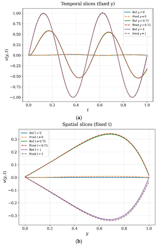
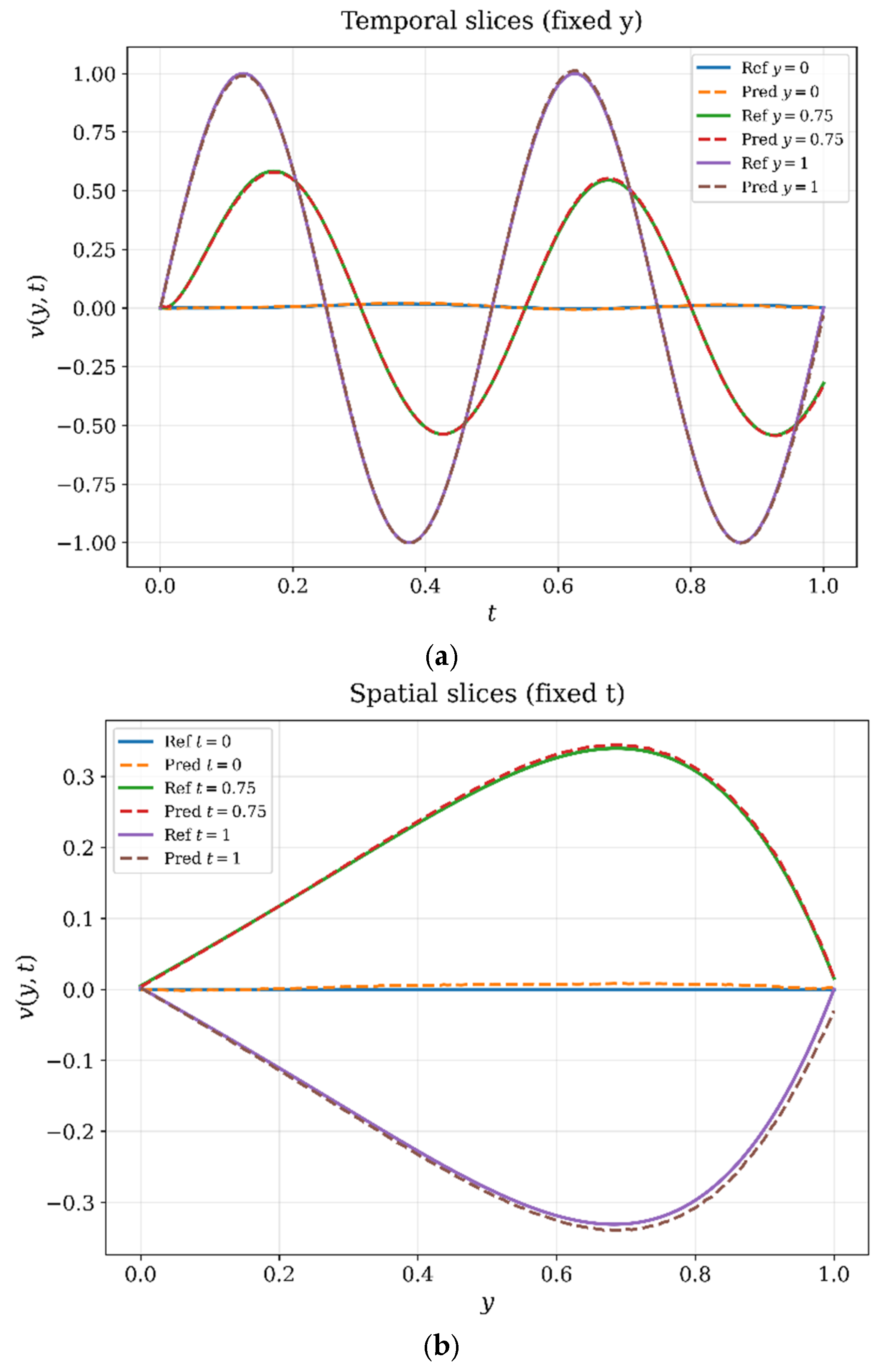
Further validation on the accuracy of the proposed PINN model is conducted using the slices of the velocity field in both the temporal and spatial dimensions illustrated in Figure 5. These slices provide a more detailed pointwise validation of the predicted solution against the reference numerical results.

Figure 5. Comparison of the PINN predictions (dashed) with the reference solution (solid) with $B=1$, ${\Lambda }_s=0.5$ and $f\left(t\right)=\mathit{sin}\left(4\pi t\right)$: (a) temporal slices of the velocity field at fixed spatial positions $y$; (b) spatial velocity profiles across the channel at selected time instances.

For the temporal slices (fixed $y$), the velocity evolution over time is examined at selected spatial locations within the channel. From the comparison, one can see that the results obtained from the PINN approach approximate the oscillatory characteristics of the numerical reference solution very well. It should be noted that not only the amplitude but also the phase of the oscillation is correctly predicted by the network.

Similarly, spatial slices (fixed $t$) are analyzed to evaluate the velocity distribution across the channel at specific time instances. There is a very good match between the predicted velocity field by the PINN algorithm and the reference solution for the entire spatial domain. The neural network accurately reproduces the smooth decay of the velocity profile from the oscillating upper boundary toward the stationary lower wall.

Thus, it can be concluded that the proposed PINN architecture successfully captures the spatio-temporal velocity field of oscillatory Couette flow. The almost perfect matching of the reference solution, which is found both in temporal and spatial sections, proves the effectiveness of the model to capture the underlying physics.

3.2. Data-Driven DeepONet

In this section, we apply the data-driven neural operator framework introduced in Section 2.3 to the Couette flow problem. A DeepONet is trained to learn the mapping from varying boundary forcing functions and slip parameters to the corresponding spatio-temporal velocity field.

3.2.1. Dataset Generation

The dataset was created through the numerical solution of the problem of Couette flow using the Crank–Nicolson method [35], implemented via GPU computation using the CuPy v14.0.0 library [40]. We produced a total of $\mathrm{10,000}$ unique simulations to ensure a miscellaneous representation of the fluid’s response. For each sample, the spatio-temporal velocity field $v\left(y, t\right)$ was evaluated on a uniform $200\times 200$ space–time grid. The overall dataset was split to $80\%$ for training, $10\%$ for testing and $10\%$ for validation.

The boundary forcing function $f\left(t\right)$, which corresponds to the moving wall velocity, was modeled as a Gaussian Random Field (GRF) [41] with a Radial Basis Function (RBF) kernel with a length scale parameter $l= 0.2$, guaranteeing smooth yet complex temporal behavior. The function f(t) was sampled at the same temporal grid points of 200.

The parametric ranges for the slip number ($B\in \left[0.1\right|100]$) and the slip relaxation number (${\Lambda }_s\in \left[0\right|0.5]$) were selected to encompass a broad range of interfacial slip and relaxation behavior. This specific interval allows the DeepONet to learn the transition from no-slip boundary conditions to significant interfacial velocity jumps, ensuring the model’s robustness across physically relevant fluid–solid interaction scenarios.

To further increase the robustness of the network in different physical regimes, the sampling of dimensionless parameters was performed using a hybrid scheme: the slip number $B$ was sampled logarithmically in the range $[0.1, 100]$ to cover three orders of magnitude of viscous dissipation, while the slip relaxation number ${\Lambda }_s$ was sampled linearly in $[0, 0.5]$. Notably, 20% of all ${\Lambda }_s$ were chosen to be zero to account for Navier slip conditions. Each numerical solution was stored as a compressed .npz file containing the discretized forcing function, the governing parameters, and the full velocity evolution field for training and validation.

3.2.2. Computational Implementation of DeepONet

The core of the proposed methodology is a DeepONet model, which is specifically optimized to handle the high-dimensional mapping from the boundary forcing functions and slip parameters to the resulting fluid flow response. Specifically, the proposed model, implemented in the TensorFlow 12/Keras 3 [42,43] framework, adopts a dual-pathway approach to decouple the input function representation from the spatio-temporal domain.

The branch network extracts the relevant features of the input data, including the boundary forcing function $f\left(t\right)$ and the slip parameters ${\Lambda }_s$ and $B$, and maps them into a latent representation. Its topology consists of four hidden layers, each containing $192$ neurons. Initially the standard Rectified Linear Unit (ReLU) was considered, but the numerical experiments indicated that it results in slower convergence and reduced accuracy in capturing the operator’s response. In contrast, the GELU [44] activation provides a smooth, non-monotonic response that proved superior for this specific task. The fact that its derivative is continuous is especially helpful because it allows the network to keep a stable and consistent flow of gradients, which is crucial for optimizing the network’s performance. This is important when you’re dealing with things that change continuously, like the way momentum spreads out in fluids.

In addition, the trunk network is responsible for processing the spatio-temporal coordinates ($y, t$). In the present implementation, the trunk’s topology is carefully balanced with that of the branch. This means it has four hidden layers of neurons of 192 neurons each. Equal width networks and setting the dimensionality of the latent space to $q=256$ guarantee that the basis functions obtained via the trunk have enough expressiveness to encode the complex structure of the extracted features. As before, the GELU activation function is used in each layer. This is important because it allows the trunk to work effectively with the branch and process the spatial and time information correctly.

We found that using four layers for each sub-network is a good balance between model capacity and generalization. It was observed through many preliminary experiments that such depth can provide sufficient non-linearity to represent the sharp velocity gradient at the boundaries, particularly when the slip number is high, while at the same time minimizing the risk of overfitting. This balanced depth-to-width ratio ensures that the network remains computationally efficient during both training and real-time inference, without compromising the spectral accuracy required for operator learning.

The last step in the architecture design is the interaction layer in which the two networks come together. This step is done using a dot product of their $q$ dimensional outputs from the latent space and then adding a trainable bias term for the final output velocity $v$. The inner product-based construction of the model enables efficient synthesis of the basis functions with the coefficients based on the input, effectively reproducing the solution to the partial differential equations across all the different parameters.

3.2.3. The Operator Validation Framework

A key component of the proposed methodology is the operator validation callback, which was developed to provide a more meaningful evaluation of the model than relying exclusively on the point-wise Mean Squared Error (MSE) loss. Although the network is trained by minimizing the standard MSE objective, its performance during validation is assessed using the relative $L_2$ error defined in Equation (20). Unlike the training loss, this metric evaluates the predictive accuracy of the operator over the complete solution field, making it more suitable for assessing the overall quality of the learned mapping.

This validation criterion is particularly useful because it is more sensitive to structural discrepancies in the predicted velocity field, allowing us to verify that the global flow behavior is accurately reproduced rather than simply matching individual data points.

To limit the additional computational cost while still monitoring the training process effectively, the operator-based validation is performed every 10 epochs. During each validation step, the model predicts the velocity field over the entire spatio-temporal domain for every sample in the validation dataset. Since evaluating the full grid requires substantial memory, the coordinate points are processed in batches of 4096, which keeps the memory usage manageable without affecting the accuracy of the evaluation.

The validation framework also includes a checkpointing mechanism that records the lowest relative $L_2$ error obtained during training. Whenever a new minimum validation error is achieved, the corresponding model weights are saved. As a result, the final model corresponds to the version that provides the best overall agreement with the underlying fluid dynamics rather than simply the lowest training loss.

3.2.4. Training Hyperparameters

A well-tuned configuration of hyperparameters enabled creating a high-performing model. The learning rate of ${10}^{-4}$ was kept constant for the whole training period to ensure that a steady exploration of a complex loss domain happened to avoid premature convergence to suboptimal minima. For training, a Monte Carlo method was used, where 4096 different spatio-temporal points were sampled at each iteration. In such a way, during 500 steps per epoch, the model sees a vast dataset of $2 \times {10}^6$ different points for each training epoch. Such a high density of sampling ensures that the neural operator is able to learn the continuity of the velocity field in the whole parametric space of upper wall velocity, slip, and slip relaxation numbers.

3.2.5. Predictive Accuracy and Convergence

To assess the consistency of the learning process, the DeepONet model was trained using five independent random seeds. Among the five independent training runs, the best model was defined as the run with the lowest relative $L_2$ error, while the median model corresponded to the run with the median relative $L_2$ error. Table 2 reports the mean and standard deviation of the operator errors obtained across these runs, together with the best performance. The model achieved a mean relative operator error of 0.355%, with a standard deviation of 0.030%, while the best performing run reached 0.297%. The small variation across the independent runs indicates consistent predictive performance with limited sensitivity to random initialization.

Table 2. Statistical performance of the proposed DeepONet architecture across five independent runs.

Metric	Mean Value	Standard Deviation	Best Achievement
Best Operator ${\mathit{L}}_2$ Error (%)	$0.355$	$0.03$	$0.297$
Training Time (min)	$256.65$	$14.91$	$238.61$

Similarly to the PINN, the DeepONet presented in the following analysis is obtained from the model with the median performance across the five independent runs.

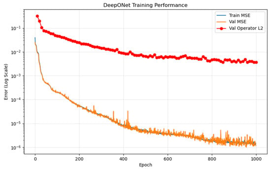
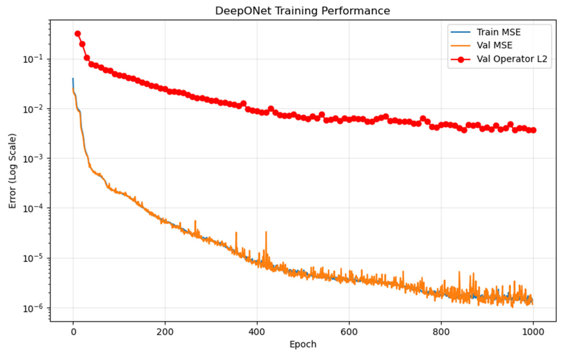
The performance of the DeepONet architecture during training is shown in Figure 6. We can see how the MSE and the operator $L_2$ error change over $1000$ epochs. Both the training and validation MSE decrease rapidly at first, going from approximately ${10}^{-1}$ to below ${10}^{-4}$ in just a few hundred epochs. This shows that the model is learning quickly and well. The fact that the training and validation losses are very similar suggests that the model is not overfitting and is generalizing well to new data. The use of the GELU activation function helps with this by making sure the gradients are smooth and easy to work with. The validation operator $L_2$ error also decreases steadily and stabilizes around $3.6\times {10}^{-3}$($\approx 0.36\%$), indicating that the network has successfully learned the underlying solution operator. In the later stages of training (approximately $600-1000$ epochs), the loss curves reach a refinement phase where the MSE approaches ${10}^{-6}$, with some small oscillations that are typical of stochastic optimization. Overall, these results demonstrate efficient and stable convergence of the DeepONet architecture.

Figure 6. Training history of the DeepONet model showing the evolution of the mean squared error (MSE) and the relative operator $L_2$ error over epochs. Both training and validation losses exhibit rapid convergence and remain closely aligned, indicating stable learning and strong generalization.

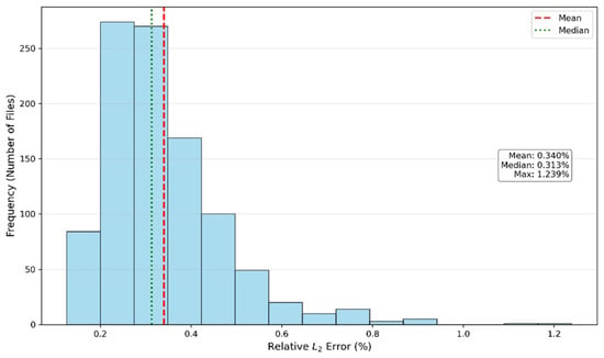
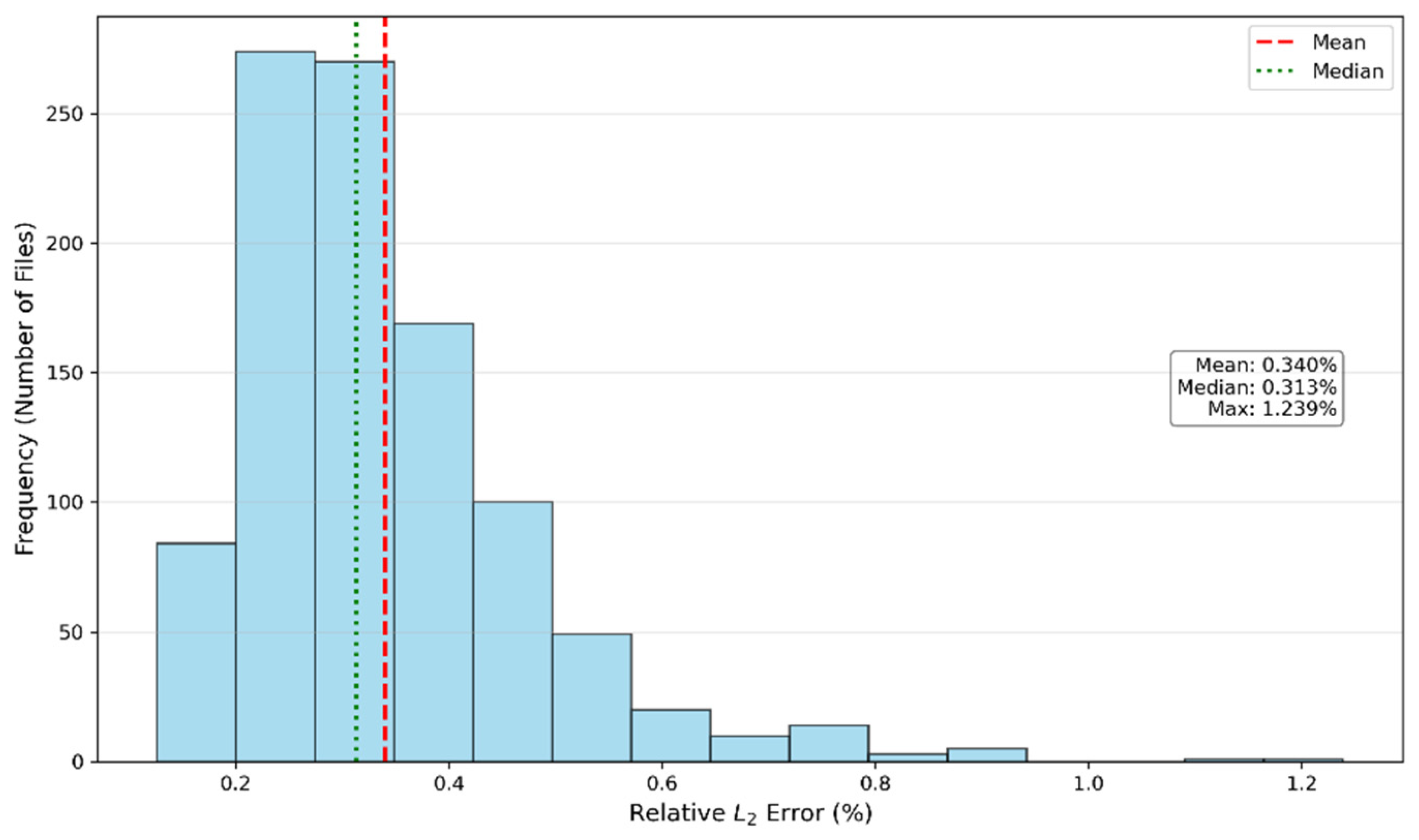
The predictive performance of the proposed DeepONet was validated against the unseen test dataset to assess its generalization capability. Figure 7 shows the distribution of the relative $L_2$ error on these samples. The high fidelity of this model can be observed by the relatively low mean error of $0.340\%$ and the median error of $0.313\%$. The error distribution is compactly concentrated, with most cases falling below $0.5\%$. Even at the tail of the distribution, the maximum recorded error is only $1.239\%$, indicating that the model provides consistent and reliable predictions across the entire parametric range of the test set.

Figure 7. Distribution of the relative $L_2$ error for DeepONet predictions on the unseen test set.

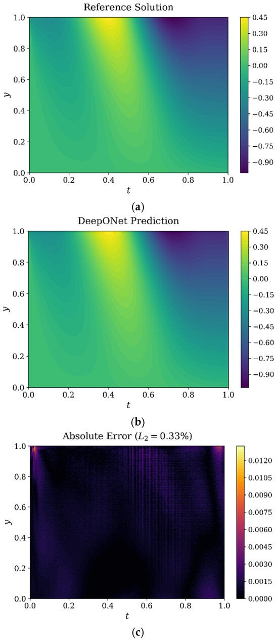
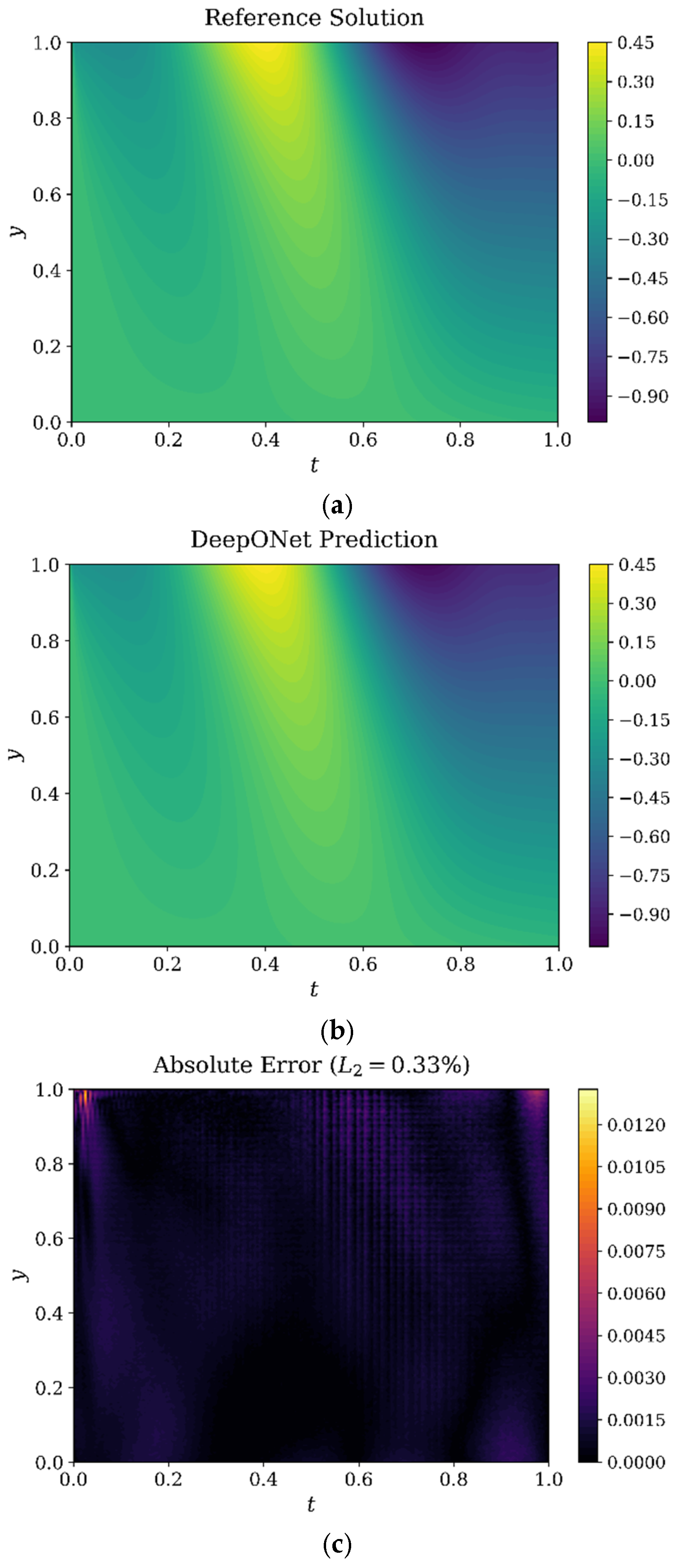
To visually demonstrate this performance, a representative sample from the unseen test set was analyzed in detail. Figure 8 presents a comparison between the reference solution and the DeepONet prediction for a representative sample from the unseen test dataset. The predicted solution closely matches the reference over the whole spatio-temporal domain and reproduces the amplitude and structure of the solution. The relative $L_2$ error is approximately $0.33\%$, which proves high predictive accuracy and good generalization ability of the learned operator. The absolute error map shows that the error remains very small over most of the domain and becomes larger in areas with steeper gradients. Similar behavior was reported by Wang et al. [17], who observed that neural operator approximations tend to exhibit higher local errors in regions with steep gradients and rapidly varying solution features. Temporal slices (fixed $y$) and spatial slices (fixed $t$) (see Figure 9) additionally prove the high coincidence between the reference and approximate solutions.

Figure 8. Results for a representative sample from the unseen test dataset with $B=11.16$ and ${\Lambda }_s=0.12$: (a) reference solution; (b) DeepONet prediction; (c) absolute $L_2$ error.

Figure 9. Comparison of the DeepONet predictions (dashed lines) with reference solutions (solid lines) with $B=11.16$ and ${\Lambda }_s=0.12$: (a) temporal slices $v\left(y,t\right)$ at fixed spatial locations; (b) spatial slices at fixed time instances.

To further evaluate the DeepONet predictions regarding the flow characteristics linked to the dynamic slip boundary condition, extra post-processing was carried out for 20 previously unseen test cases. Because the current DeepONet is trained in a purely data-driven way, the governing equation and its initial and boundary conditions are not directly enforced as residual terms during training. Still, the predicted velocity fields reproduce the behavior at the slipping wall with quite good accuracy. Specifically, the median relative errors in the slip velocity and the wall shear rate, when compared with the numerical reference solutions, were 1.45% and 2.89%, respectively. Additionally, the normalized residual of the dynamic slip boundary condition showed a median value of 6.09%. The deviations related to the set upper wall and initial conditions were also small, with median normalized values of 4.48% and 0.70%, respectively. These findings add to the global relative $L_2$ error analysis and show that the accuracy of the predicted velocity fields is also present in the boundary behavior of the flow. As expected for a data-driven model, quantities that involve derivatives are more sensitive to small local prediction errors.

3.2.6. Generalization Under a Distribution Shift in the Boundary Forcing Profile

To evaluate the robust generalization of the DeepONet, we introduce a distribution shift in the boundary forcing, replacing the stochastic Gaussian Random Field (GRF) input with a deterministic sinusoidal velocity profile $f\left(t\right)=\sin \left(4\pi t\right)$, while keeping the physical parameters ($B,{\Lambda }_s$) within their training bounds.

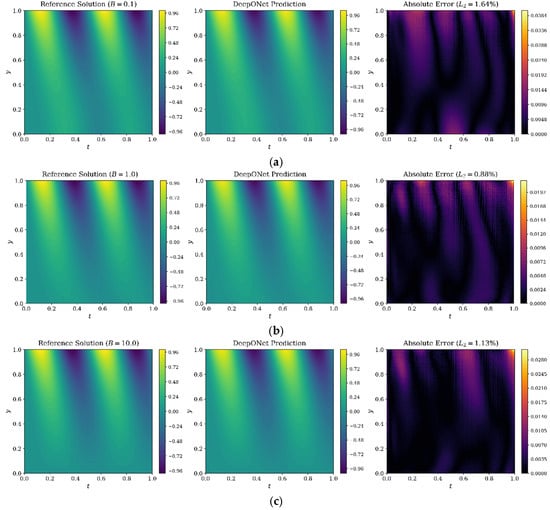
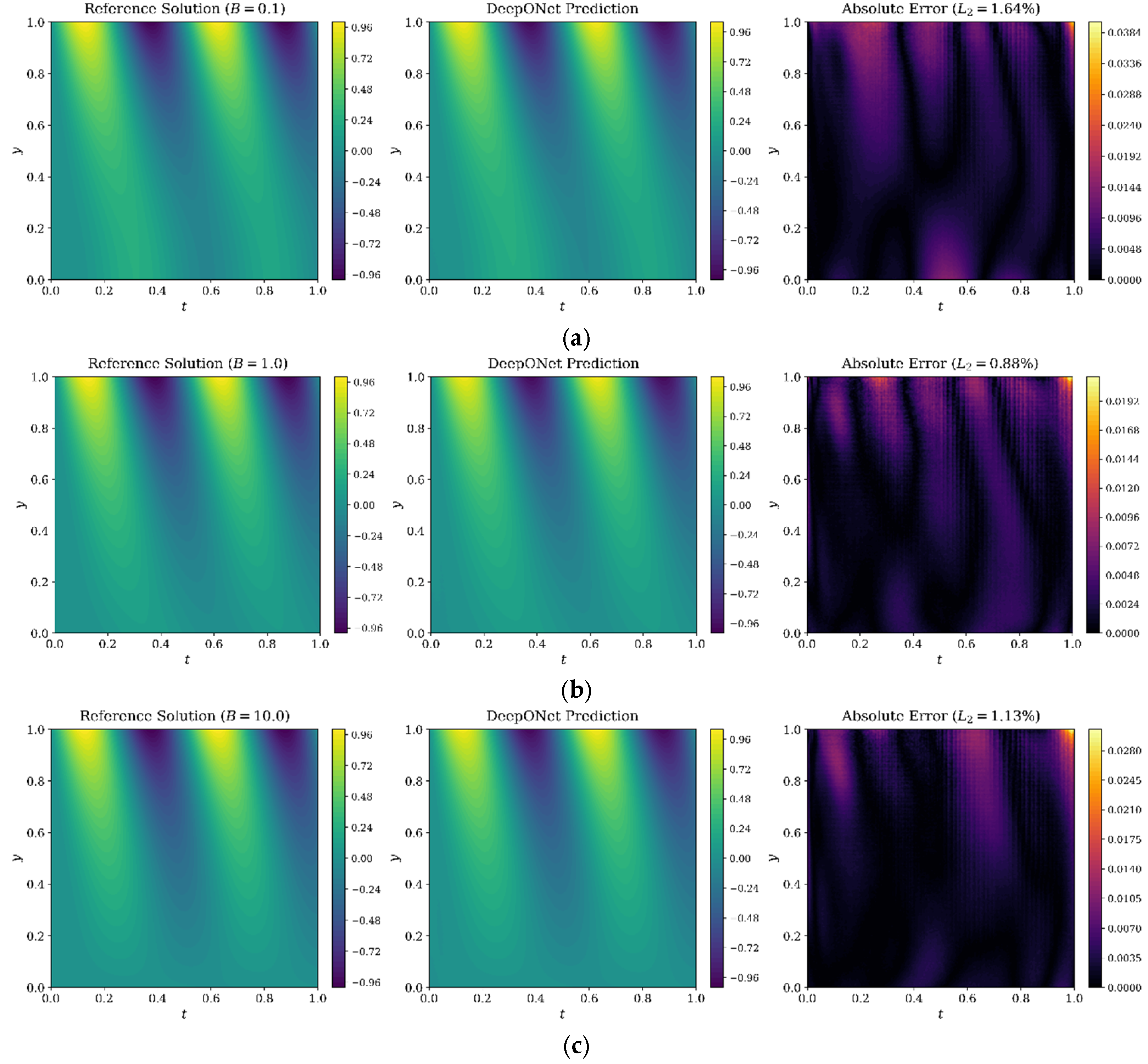
Figure 10 presents the comparative heatmaps for $B=0.1$, 1 and $10$ with ${\Lambda }_s=0.5$. The predicted results from DeepONet are in great agreement with the numerical solution at the reference solution over all the parameter domains. The relative $L_2$ error stays very low from $0.88\%$ to $1.64\%$. It is worth mentioning that the absolute error maps show that the accuracy of the model still holds true even for $B=0.1$, where the velocity gradients near the boundaries are most pronounced due to the slip conditions.

Figure 10. Generalization capability of DeepONet on unseen harmonic signals ($f\left(t\right)=sin\left(4\pi t\right)$). Comparative heatmaps for (a) $B = 0.1$, (b) $B = 1$, (c) $B = 10$ with ${\Lambda }_s=0.5$.

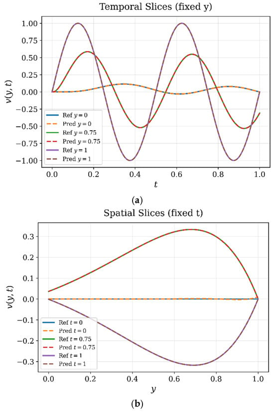
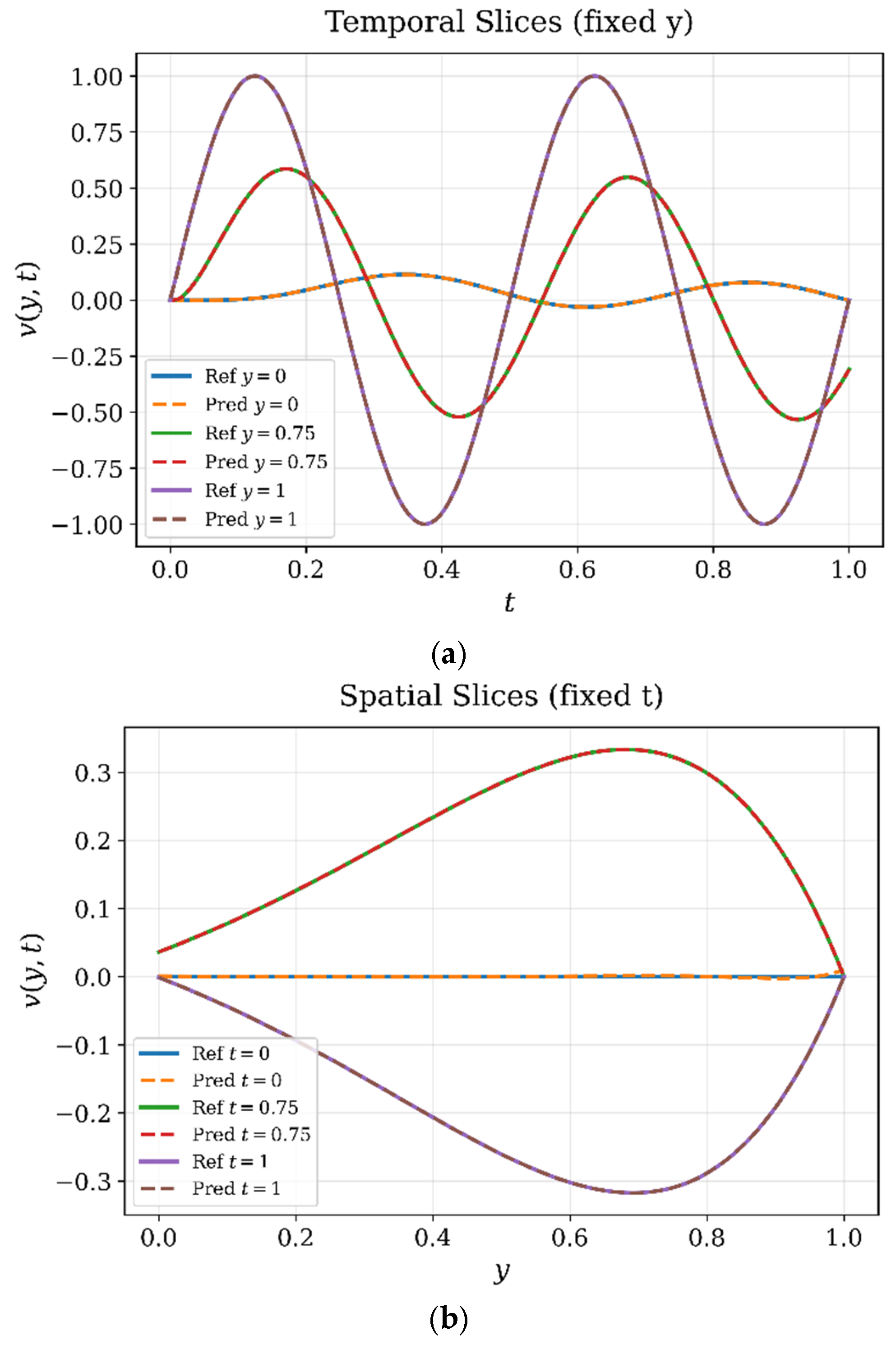
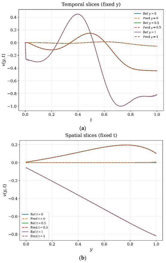
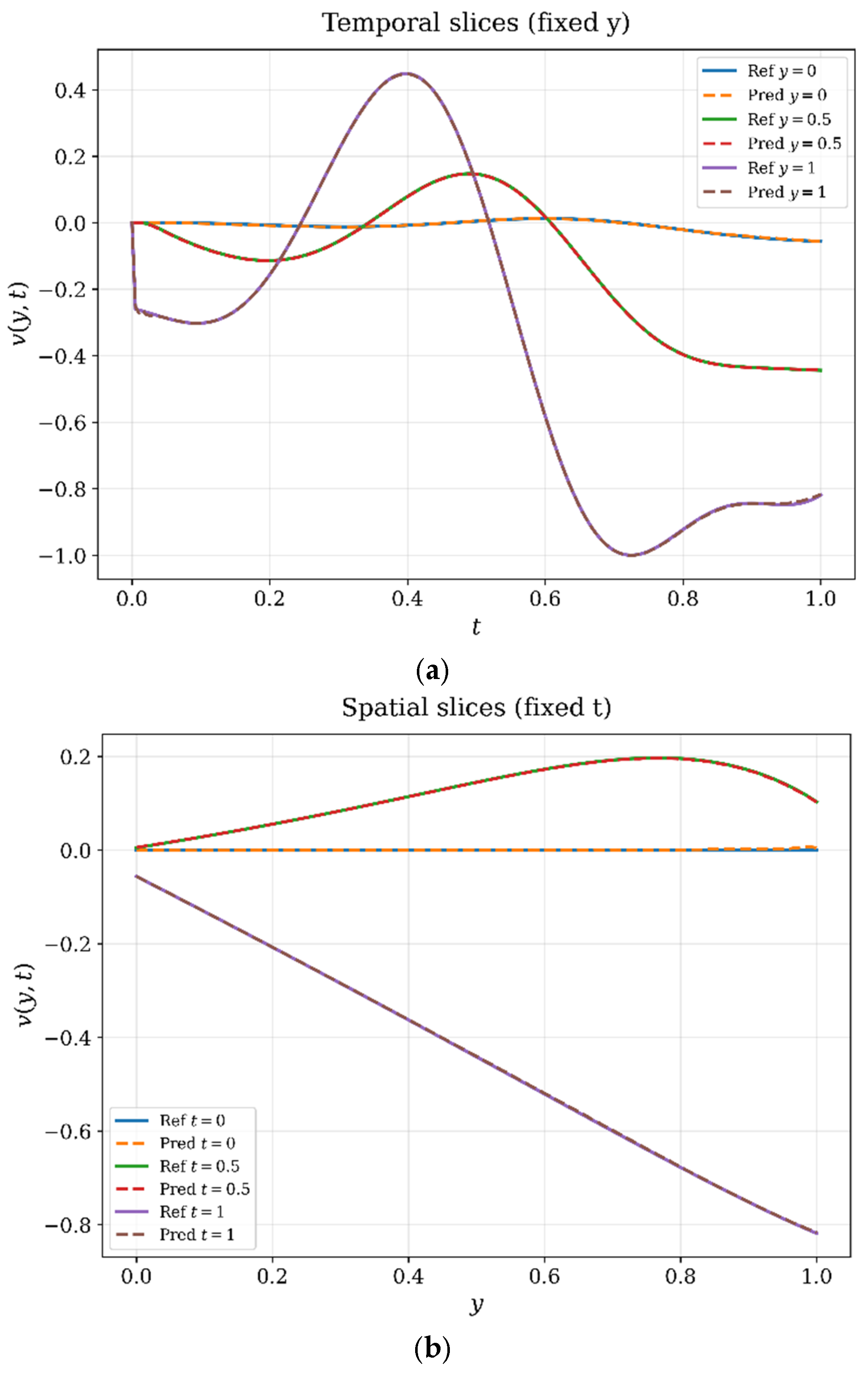
Further support for the structural consistency of the estimated velocity field comes from the spatial and temporal slices (Figure 11). Indeed, in the temporal slices (fixed $y$), the DeepONet reproduces the frequency and phase of the oscillating flow with great accuracy and follows the $4\pi t$ harmonic profile. Similarly, the spatial slices (fixed $t$) show near-perfect coincidence between the estimated and reference profiles (dashed vs. solid lines). Thus, it is evident that the DeepONet learned to recover the boundary layer dynamics at $y=0$ and $1$, indicating the successful learning of the physical constraints and the underlying operator of the oscillating fluid system.

Figure 11. Results for $B=10 and {\Lambda }_s=0.5$ demonstrating near-perfect alignment between the reference solution (solid lines) and DeepONet predictions (dashed lines): (a) temporal slices; (b) spatial slices.

These results indicate that the learned operator retains good predictive accuracy for the investigated harmonic boundary forcing, despite the change from the GRF-based forcing functions used during training.

3.3. Discussion

The PINN and DeepONet results show that these two learning methods are designed for fundamentally different tasks. PINN is trained to address a specific flow configuration, while DeepONet is built to learn the solution operator across a variety of boundary forcing functions and slip parameters. Therefore, their performance should be assessed based on these distinct learning objectives rather than by making a direct comparison between equivalent models.

In the case examined with PINN, a relative error of 0.083% was achieved. This high precision is expected, as PINNs function as mesh-free solvers optimized for a specific set of parameters and forcing functions, directly enforcing the underlying partial differential equations (PDEs) during training. However, this accuracy comes at a significant computational cost when multiple problem instances are considered. In contrast, DeepONet achieved a mean relative error of 0.340% on the standard test set. It serves as a reusable operator-based surrogate, allowing for instant predictions of the solution for any combination from the parametric space, without the need for additional training or solving the equations again.

Table 3 presents the performance data of all three methods. All timing measurements were carried out in a Google Colab environment. The Crank–Nicolson (CN) method was implemented using a tridiagonal solver, with matrix factorization reused throughout the time integration. Its execution time was recorded on a CPU. The inference times for both PINN and DeepONet were measured on an NVIDIA T4 GPU after warm-up and synchronization. Therefore, the times given should be seen as wall-clock measurements for the respective hardware, not as direct hardware-equivalent speedups.

Table 3. Predictive accuracy and representative wall-clock execution times for the three methods.

Method	Hardware	Rel. ${\mathit{L}}_2$ Error (%)	Representative Execution Time (ms)
CN	CPU	Reference	4.05
PINN	GPU	0.083 (specific case)	1.80
DeepONet	GPU	0.340 (test-set mean)	2.36

For the present problem, the optimized CN solver took about 4.05 ms per solution, compared with 1.80 ms for PINN and 2.36 ms for DeepONet. Thus, in the computational setup used in this study, the trained DeepONet provided predictions in approximately half the wall-clock time required by the optimized CN solver. More importantly, once trained, DeepONet can be applied repeatedly to different boundary forcing functions and slip parameters without retraining or re-solving the governing equations. This combination of low inference time and model reusability is the main computational advantage of the operator learning approach for repeated parametric evaluations.

4. Conclusions

In this work, we investigated Physics-Informed Neural Networks (PINNs) and data-driven Deep Operator Networks (DeepONets) for solving the Newtonian plane Couette flow with dynamic wall slip. The two approaches address different learning objectives: PINN provides an accurate solution for a specific flow configuration, whereas DeepONet learns a solution operator over a range of boundary forcing functions and slip parameters.

For the specific case considered in this study, PINN achieved a relative $L_2$ error of 0.083%. On the other hand, DeepONet achieved a mean relative $L_2$ error of 0.340% over the standard test set. In addition, DeepONet demonstrated high predictive accuracy for unseen GRF test samples and retained good accuracy when evaluated with a deterministic harmonic forcing not used in the GRF-based dataset.

The main advantage of DeepONet is its ability to perform repeated parametric evaluations. Although generating the training data and training the operator require an initial computational investment, the trained DeepONet provides rapid inference for new inputs without retraining. In the present computational setup, its representative inference time was 2.36 ms per solution, compared with 4.05 ms for the optimized Crank–Nicolson solver. Since the DeepONet and CN calculations were performed on GPU and CPU, respectively, these values represent device-specific wall-clock measurements rather than hardware-equivalent speedups. Together with its low inference time, the ability to evaluate different inputs without retraining makes DeepONet well suited for repeated parametric studies.

Overall, the results highlight the complementary roles of physics-informed solution learning and data-driven operator learning for transient flows with dynamic wall slip.

Future work will explore the integration of physics-informed losses within DeepONet architecture to further enhance its accuracy while maintaining its operational speed and the extension of the method to higher dimensional flows, e.g., transient Poiseuille flow in a square channel [15], or non-Newtonian channel flows of varying cross-section [45], reducing data requirements through hybrid training strategies.

References

- Hatzikiriakos, S.G. Wall Slip of Molten Polymers. Prog. Polym. Sci. 2012, 37, 624–643. [Google Scholar] [CrossRef] [Scilit]
- Lauga, E.; Brenner, M.; Stone, H. Microfluidics: The No-Slip Boundary Condition. In Springer Handbook of Experimental Fluid Mechanics; Tropea, C., Yarin, A.L., Foss, J.F., Eds.; Springer: Berlin/Heidelberg, Germany, 2007; pp. 1219–1240. [Google Scholar]
- Brunton, S.L. Applying Machine Learning to Study Fluid Mechanics. Acta Mech. Sin. 2021, 37, 1718–1726. [Google Scholar] [CrossRef] [Scilit]
- Wang, H.; Cao, Y.; Huang, Z.; Liu, Y.; Hu, P.; Luo, X.; Song, Z.; Zhao, W.; Liu, J.; Sun, J.; et al. Recent Advances on Machine Learning for Computational Fluid Dynamics: A Survey. arXiv 2024, arXiv:2408.12171. [Google Scholar]
- Li, Y.; Chang, J.; Kong, C.; Bao, W. Recent Progress of Machine Learning in Flow Modeling and Active Flow Control. Chin. J. Aeronaut. 2022, 35, 14–44. [Google Scholar] [CrossRef] [Scilit]
- Catsoulis, S.; Singh, J.-S.; Narayanan, C.; Lakehal, D. Integrating Supervised Learning and Applied Computational Multi-Fluid Dynamics. Int. J. Multiph. Flow 2022, 157, 104221. [Google Scholar] [CrossRef] [Scilit]
- Sun, X.; Cao, W.; Shan, X.; Liu, Y.; Zhang, W. A Generalized Framework for Integrating Machine Learning into Computational Fluid Dynamics. J. Comput. Sci. 2024, 82, 102404. [Google Scholar] [CrossRef] [Scilit]
- Zhang, C.; Zhou, Y.; Li, J.; Chu, S.; Qin, Q.; Huang, L. Data-Driven Prediction of Wave Response for a Modular Floating Solar Array. Ocean Eng. 2026, 349, 124192. [Google Scholar] [CrossRef] [Scilit]
- Raissi, M.; Perdikaris, P.; Karniadakis, G.E. Physics-Informed Neural Networks: A Deep Learning Framework for Solving Forward and Inverse Problems Involving Nonlinear Partial Differential Equations. J. Comput. Phys. 2019, 378, 686–707. [Google Scholar] [CrossRef] [Scilit]
- Cai, S.; Mao, Z.; Wang, Z.; Yin, M.; Karniadakis, G.E. Physics-Informed Neural Networks (PINNs) for Fluid Mechanics: A Review. Acta Mech. Sin. 2021, 37, 1727–1738. [Google Scholar] [CrossRef] [Scilit]
- Tao, Z.; Xu, K.; Liu, F. LSTM-PINN: An Hybrid Method for Prediction of Steady-State Electrohydrodynamic Flow. J. Comput. Phys. 2026, 548, 114586. [Google Scholar] [CrossRef] [Scilit]
- Ra, D.; Lee, J.; Lee, M.; Kwak, S.; Lee, S.; Lee, S. Physics-Informed Machine Learning across Manufacturing Processes: Recent Advances, Challenges, and Directions. J. Manuf. Syst. 2026, 85, 72–95. [Google Scholar] [CrossRef] [Scilit]
- Kovachki, N.; Li, Z.; Liu, B.; Azizzadenesheli, K.; Bhattacharya, K.; Stuart, A.; Anandkumar, A. Neural Operator: Learning Maps between Function Spaces with Applications to Pdes. J. Mach. Learn. Res. 2023, 24, 1–97. [Google Scholar]
- Li, H.; Miao, Y.; Khodaei, Z.S.; Aliabadi, M.H. An Architectural Analysis of DeepOnet and a General Extension of the Physics-Informed DeepOnet Model on Solving Nonlinear Parametric Partial Differential Equations. Neurocomputing 2025, 611, 128675. [Google Scholar] [CrossRef] [Scilit]
- Eshaghi, M.S.; Valizadeh, N.; Anitescu, C.; Wang, Y.; Zhuang, X.; Rabczuk, T. Multi-Head Neural Operator for Modelling Interfacial Dynamics. Int. J. Mech. Sci. 2026, 317, 111363. [Google Scholar] [CrossRef] [Scilit]
- Lu, L.; Jin, P.; Pang, G.; Zhang, Z.; Karniadakis, G.E. Learning Nonlinear Operators via DeepONet Based on the Universal Approximation Theorem of Operators. Nat. Mach. Intell. 2021, 3, 218–229. [Google Scholar] [CrossRef] [Scilit]
- Wang, S.; Wang, H.; Perdikaris, P. Learning the Solution Operator of Parametric Partial Differential Equations with Physics-Informed DeepONets. Sci. Adv. 2021, 7, eabi8605. [Google Scholar] [CrossRef] [Scilit] [PubMed]
- Koric, S.; Abueidda, D.W. Data-Driven and Physics-Informed Deep Learning Operators for Solution of Heat Conduction Equation with Parametric Heat Source. Int. J. Heat Mass Transf. 2023, 203, 123809. [Google Scholar] [CrossRef] [Scilit]
- Jiao, A.; Yan, Q.; Harlim, J.; Lu, L. Solving Forward and Inverse PDE Problems on Unknown Manifolds via Physics-Informed Neural Operators. arXiv 2024, arXiv:2407.05477. [Google Scholar]
- Belmonte, R.; Dieulot, J.-Y.; Galanti, M.; Van Sint Annaland, M. Physics-Informed Artificial Intelligence with Splines for Modeling Advection–Diffusion–Reaction under Dynamic Boundaries. Digit. Eng. 2026, 9, 100083. [Google Scholar] [CrossRef] [Scilit]
- Denn, M.M. Extrusion Instabilities and Wall Slip. Annu. Rev. Fluid Mech. 2001, 33, 265–287. [Google Scholar] [CrossRef] [Scilit]
- Malkin, A.Y.; Patlazhan, S.A. Wall Slip for Complex Liquids–Phenomenon and Its Causes. Adv. Colloid Interface Sci. 2018, 257, 42–57. [Google Scholar] [CrossRef] [Scilit] [PubMed]
- Neto, C.; Evans, D.R.; Bonaccurso, E.; Butt, H.-J.; Craig, V.S.J. Boundary Slip in Newtonian Liquids: A Review of Experimental Studies. Rep. Prog. Phys. 2005, 68, 2859–2897. [Google Scholar] [CrossRef] [Scilit]
- Abbasi Moud, A.; Piette, J.; Danesh, M.; Georgiou, G.C.; Hatzikiriakos, S.G. Apparent Slip in Colloidal Suspensions. J. Rheol. 2022, 66, 79–90. [Google Scholar] [CrossRef] [Scilit]
- Hatzikiriakos, S.G. Slip Mechanisms in Complex Fluid Flows. Soft Matter 2015, 11, 7851–7856. [Google Scholar] [CrossRef] [Scilit] [PubMed]
- Navier, C. Mémoire Sur Les Lois Du Mouvement Des Fluides. Mém. l’Acad. R. Sci. l’Institut Fr. 1823, 6, 389–440. [Google Scholar]
- Pearson, J.R.A.; Petrie, C.J.S. On the Melt-Flow Instability of Extruded Polymers. In Proceedings of the 4th International Rheological Congress, Providence, RI, USA, 26–30 August 1963; 3., pp. 265–282. [Google Scholar]
- Hatzikiriakos, S.G.; Kalogerakis, N. A Dynamic Slip Velocity Model for Molten Polymers Based on a Network Kinetic Theory. Rheol. Acta 1994, 33, 38–47. [Google Scholar] [CrossRef] [Scilit]
- Ebrahimi, M.; Konaganti, V.K.; Hatzikiriakos, S.G. Dynamic Slip of Polydisperse Linear Polymers Using Partitioned Plate. Phys. Fluids 2018, 30, 030601. [Google Scholar] [CrossRef] [Scilit]
- Thalakkottor, J.J.; Mohseni, K. Analysis of Boundary Slip in a Flow with an Oscillating Wall. Phys. Rev. E—Stat. Nonlinear Soft Matter Phys. 2013, 87, 033018. [Google Scholar] [CrossRef] [Scilit]
- Kazatchkov, I.B.; Hatzikiriakos, S.G. Relaxation Effects of Slip in Shear Flow of Linear Molten Polymers. Rheol. Acta 2010, 49, 267–274. [Google Scholar] [CrossRef] [Scilit]
- Kaoullas, G.; Georgiou, G.C. Start-up and Cessation Newtonian Poiseuille and Couette Flows with Dynamic Wall Slip. Meccanica 2015, 50, 1747–1760. [Google Scholar] [CrossRef] [Scilit]
- Farragui, M.E.; Souhar, O.; Georgiou, G.C. Newtonian Annular Poiseuille and Couette Flows with Dynamic Wall Slip. Eur. J. Mech.-B/Fluids 2024, 103, 136–144. [Google Scholar] [CrossRef] [Scilit]
- El Farragui, M.; Souhar, O.; Georgiou, G.C. Transient Newtonian Poiseuille Flow in a Square Channel with Dynamic Wall Slip. Phys. Fluids 2025, 37, 023144. [Google Scholar] [CrossRef] [Scilit]
- Abou Hasan, M.M.; Ahmed, E.A.A.; Ghaleb, A.F.; Abou-Dina, M.S.; Georgiou, G.C. Numerical Solution of the Newtonian Plane Couette Flow with Linear Dynamic Wall Slip. Fluids 2024, 9, 172. [Google Scholar] [CrossRef] [Scilit]
- Kingma, D.P.; Ba, J. Adam: A Method for Stochastic Optimization. arXiv 2014, arXiv:1412.6980v9. [Google Scholar]
- Liu, D.C.; Nocedal, J. On the Limited Memory BFGS Method for Large Scale Optimization. Math. Program. 1989, 45, 503–528. [Google Scholar] [CrossRef] [Scilit]
- Bora, A.; Dai, W.; Wilson, J.P.; Boyt, J.C. Neural Network Method for Solving Parabolic Two-Temperature Microscale Heat Conduction in Double-Layered Thin Films Exposed to Ultrashort-Pulsed Lasers. Int. J. Heat Mass Transf. 2021, 178, 121616. [Google Scholar] [CrossRef] [Scilit]
- Omrani, M.; Nematollahi, M.; Ghassemi, M. Modeling Interacting Convection Regimes with PINNs: Improving Vanilla Architecture Performance with Minimal Supervision. Int. Commun. Heat Mass Transf. 2026, 172, 110763. [Google Scholar] [CrossRef] [Scilit]
- Okuta, R.; Unno, Y.; Nishino, D.; Hido, S.; Loomis, C. CuPy: A NumPy-Compatible Library for NVIDIA GPU Calculations. In Proceedings of the Workshop on Machine Learning Systems (LearningSys); NeurIPS: Long Beach, CA, USA, 2017. [Google Scholar]
- Rasmussen, C.E.; Williams, C.K.I. Gaussian Processes for Machine Learning; The MIT Press: Cambridge, MA, USA, 2005. [Google Scholar]
- Abadi, M.; Agarwal, A.; Barham, P.; Brevdo, E.; Chen, Z.; Citro, C.; Corrado, G.S.; Davis, A.; Dean, J.; Devin, M.; et al. TensorFlow: Large-Scale Machine Learning on Heterogeneous Distributed Systems. arXiv 2016, arXiv:1603.04467. [Google Scholar]
- Chollet François et al, Keras 2015. Available online: https://github.com/keras-team/keras (accessed on 1 June 2026).
- Hendrycks, D.; Gimpel, K. Gaussian Error Linear Units (GELUs). arXiv 2016, arXiv:1606.08415. [Google Scholar]
- Garg, A.; Prasad, P. Yield–Stress Shear Thinning and Shear Thickening Fluid Flows in Deformable Channels. Phys. Scr. 2024, 99, 035240. [Google Scholar] [CrossRef] [Scilit]
Disclaimer/Publisher’s Note: The statements, opinions and data contained in all publications are solely those of the individual author(s) and contributor(s) and not of MDPI and/or the editor(s). MDPI and/or the editor(s) disclaim responsibility for any injury to people or property resulting from any ideas, methods, instructions or products referred to in the content. |
© 2026 by the authors. Licensee MDPI, Basel, Switzerland. This article is an open access article distributed under the terms and conditions of the Creative Commons Attribution (CC BY) license.