Wall-Resolved Large-Eddy Simulation of an Airfoil Using High-Order Spectral Element CFD Solver NEKO

Abstract

This study employs wall-resolved Sigma SGS Large-Eddy Simulation (WR-LES) of the Eppler 387 airfoil to evaluate the higher-order Spectral Element Method (SEM) CFD solver NEKO at a moderate Reynolds number of 10⁵ and an angle of attack of 4 degrees. 2.5D simulation is performed with a span of 10% chord length using a polynomial order of 3, resulting in 300,960 elements and approximately 19 million Gauss-Lobatto-Legendre (GLL) quadrature points. Aerodynamic force coefficients and pressure distribution along the airfoil are used to evaluate the SEM solver and to validate results against wind-tunnel experimental data from NASA Technical Memorandum 4062 and OpenFOAM 2D RANS (simpleFoam) simulations (k-$\omega$ SST, k-$\omega$ SST Langtry–Menter, and k-$\omega$ SST CND). NEKO predicts the pressure distribution in good agreement with the experimental results; however, the transition point is captured slightly downstream of the experimentally observed location. The solver predicts the lift coefficient matching experimental values up to the 3rd decimal place, but the drag is overestimated. This discrepancy may be attributed to the absence of inflow turbulence in the numerical setup, which is likely present in the wind-tunnel experiment. This study demonstrates both the potential and limitations of higher-order SEM solver NEKO for CFD simulation.

1. Introduction

Airfoil aerodynamics is strongly influenced by separated flow structures and turbulent wake dynamics. Capturing these complex phenomena requires accurate numerical approaches capable of resolving both near-wall features and turbulent structures. Aerodynamic performance of an airfoil depends on its geometric and operating parameters, which influence the resulting flow characteristics and aerodynamic forces. Modifying airfoil parameters such as thickness, chord length, span length, and the angle of attack can result in variations in lift and drag forces, wake formation, and flow separation and reattachment. To obtain insights into airfoil performance, wind tunnel experiments were commonly used in the past [1]. While these experiments provide real physical results, the process is expensive and time-consuming [2]. Consequently, Computational Fluid Dynamics (CFD) has become an alternative, offering detailed visualization and analysis of the flow. Unsteady and separated flows demand high-fidelity simulations such as Direct Numerical Simulations (DNS) and Wall-Resolved Large-Eddy Simulations (WRLES). Compared to WRLES, Wall-Modeled Large-Eddy Simulation (WMLES) uses a wall model to reduce near-wall grid requirements and is computationally less expensive [3]. Technological advancements in numerical techniques and computational power are further expanding CFD capabilities and applications [4,5].

At low Reynolds numbers, the flow over an airfoil is dominated by the laminar separation bubble (LSB). Laminar boundary layer separates, transitions to turbulence in the detached shear layer, and reattaches as a turbulent boundary layer. The size and position of this bubble largely determine the lift and drag; therefore, accurately reproducing these are the principal difficulty of these flows. These characteristics are highly sensitive to both the turbulence treatment and the disturbance environment [6,7]. Accurately resolving these complex transitional flow phenomena requires high-fidelity numerical approaches with sufficient spatial and temporal resolution, making high-order and spectral-element discretisations particularly attractive for wall-resolved large eddy simulations. Beck et al. [8] applied high-order discontinuous Galerkin spectral-element methods for transitional and turbulent flow simulations, and Tonicello et al. [9] applied a spectral-difference method with an explicit dynamic subgrid-scale model to transitional low-Reynolds-number airfoil flow. The predicted bubble is nonetheless sensitive to how the unresolved scales are treated, as shown by Garmann et al. [10] in comparing implicit LES with explicit subgrid-scale-model LES for low-Reynolds-number airfoils. For the Eppler 387 specifically, Gross et al. [6] performed large-eddy simulations at $Re={10}^5$ and found that introducing $1\%$ freestream turbulence advanced reattachment and reduced the length of the separated region, improving agreement with experiment. Wall-resolved LES of the Eppler 387 with an explicit subgrid-scale closure in a spectral-element solver such as NEKO has not previously been reported, which motivates the present study.

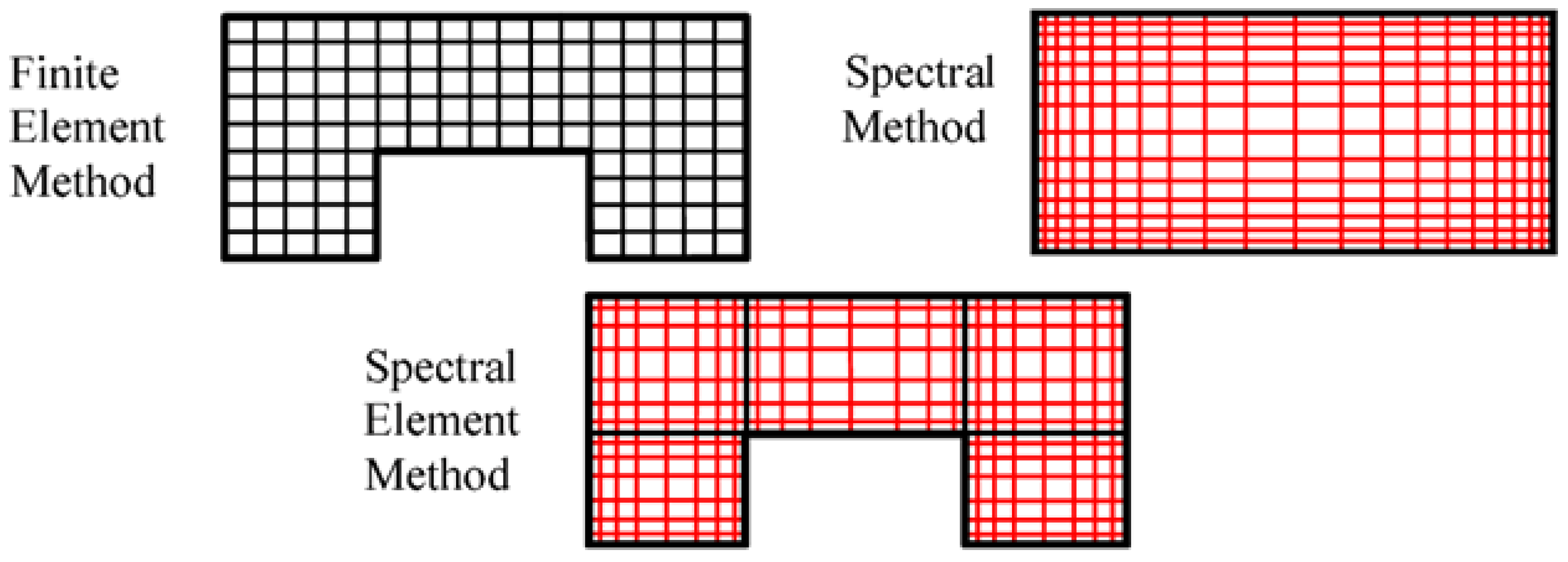
High-order numerical methods such as Spectral Element Method (SEM) have demonstrated advantages over traditional numerical methods [11] and show good agreement with experimental data [12]. SEM employs high-degree polynomial basis functions, such as Legendre or Chebyshev polynomials, enabling spectral convergence and exponential accuracy [13] while requiring fewer elements than the low-order methods. They perform well on coarser meshes and scale efficiently on parallel and GPU systems, though at higher memory and computational costs [14]. SEM efficiency is further enhanced by its compatibility with high-performance computing architectures, supporting large-scale simulations with substantial speedups [15]. SEM combines the geometric flexibility of the finite element method (FEM) with the exponential accuracy of spectral methods (Figure 1). Discretization in SEM relies on both h and p refinement, whereas h refinement is the only parameter in low-order mesh generation. SEM offers a high-order discretization strategy, enabling refinement through an increase in polynomial order without altering the underlying mesh. High-order methods are particularly sensitive to mesh quality and therefore require carefully structured and smooth grids. In this study, the mesh is generated using Gmsh, which provides precise control over the elements, while Nek5000’s mesh smoothening utility further enhances the quality through nodal displacement. Polynomial order selected for this simulation provides the required number of inner nodes (GLL) in the spanwise direction, consistent with other typical wall-resolved LES simulations  [3]. Results obtained with NEKO are cross-compared against OpenFOAM k–$\omega$ SST, k–$\omega$ SST Langtry–Menter, and k–$\omega$ SST–CND RANS models with simpleFoam solver, as well as experimental results, to establish a benchmark for numerical simulation.

NEKO, an incompressible SEM Navier–Stokes solver and an evolution of Nek5000, is a modern high-performance CFD code written in object-oriented Fortran. It optimizes memory management, supports multi-tier solver abstractions, and efficiently leverages diverse hardware architectures and accelerators for large-scale simulations [17]. NEKO’s underlying high-order solver has been verified and applied to turbulent flows in prior work: it has been verified against the Taylor–Green vortex benchmark through cross-comparison with Nek5000 and NekRS [17], and has been employed for large-scale direct numerical simulations [15]. The combination of higher-order spectral element schemes with wall-resolved LES enables effective capture of flow separation and scale resolution. Although WRLES imposes high computational cost constraints, parallelization through high-order methods helps to mitigate this drawback, motivating the use of HPC clusters for the present simulations. This work contributes to the understanding of scale resolved physics of high-order SEM in wall-resolved LES simulations of Eppler 387 airfoil using NEKO, thereby highlighting the potential benefits and limitations of the solver. The performance of NEKO’s newly implemented LES module is examined using the Sigma Sub-Grid Scale (SGS) model, with emphasis on its ability to resolve turbulence and calculate aerodynamic characteristics. Accuracy and performance are assessed to provide insight into the trade-off between resolution and computational cost, highlighting NEKO’s potential as a reliable tool for investigating aero–fluid dynamic problems.

2. Numerical Methods

The mass and momentum conservation equations provide a general framework for describing fluid flow. In this study, the flow under consideration has a Mach number below 0.3 and is hence treated as incompressible flow. As a result, density and viscosity remain constant, simplifying the governing equations. Consequently, the mass and momentum conservation equations are rewritten in their reduced form:

$${\displaystyle \frac{\partial u_i}{\partial x_i}}=0$$

(1)

$$\rho \left({\displaystyle \frac{\partial u_i}{\partial t}}+u_j{\displaystyle \frac{\partial u_i}{\partial x_j}}\right)=-{\displaystyle \frac{\partial p}{\partial x_i}}+\mu {\displaystyle \frac{{\partial }^2{u}_i}{\partial x_j\partial x_j}}+\rho f_i$$

(2)

Repeated indices imply summation, where $i,j=1,2,3$. Here, $u_i$ are the components of the velocity vector $\mathbf{u}$, p is the pressure, $\rho$ is the fluid density, $\mu$ is the dynamic viscosity, and $f_i$ are the components of the body-force vector $\mathbf{f}$.

2.1. WR-LES and SIGMA SGS Model

Turbulent energy cascade describes the transfer of kinetic energy from large, unstable eddies to smaller ones, continuing until the Kolmogorov scales are reached, where viscous effects dominate and turbulence dissipates as heat [18]. This multiscale nature of turbulence provides the physical basis for the LES approach, in which the larger, energy-containing scales are explicitly resolved, while the influence of the unresolved scales is modeled using subgrid-scale (SGS) models. The separation between resolved and unresolved scales is introduced through a spatial filtering operation characterized by a cutoff width [19]. This allows LES to capture the dominant turbulent physics at significantly lower computational cost than DNS. WR-LES employs extremely fine near-wall grids to resolve the viscous sublayer and buffer layer, enabling accurate prediction of attachment, separation, reattachment, and vortical structures. Unlike WM-LES, which introduces modeling uncertainty near the wall, WR-LES behaves similar to DNS in wall regions and as LES away from the wall.

When the viscosity is varying in space, for example in the LES model, the viscous stress tensor cannot be simplified and the following equations are solved in a coupled manner, the so-called stress formulation in NEKO:

$$\rho \left({\displaystyle \frac{\partial u_i}{\partial t}}+u_j{\displaystyle \frac{\partial u_i}{\partial x_j}}\right)=-{\displaystyle \frac{\partial p}{\partial x_i}}+{\displaystyle \frac{\partial }{\partial x_j}}\left({\mu }_{\mathrm{tot}}\left({\displaystyle \frac{\partial u_i}{\partial x_j}}+{\displaystyle \frac{\partial u_j}{\partial x_i}}\right)\right)+\rho f_i$$

(3)

where, ${\mu }_{\mathrm{tot}}=\mu +{\mu }_t$.

${\mu }_{\mathrm{tot}}$ is the total viscosity field, potentially including the contribution from the turbulence modelling. Repeated indices imply summation, where $i,j=1,2,3$.

In LES SGS modelling, turbulent viscosity, ${\nu }_t$ represents momentum transfer due to unresolved turbulence. Nicoud et al. [20] introduced the Sigma SGS model, in which the subgrid viscosity is defined based on the singular values of the velocity gradient tensor, rather than relying solely on the magnitude of the strain-rate tensor as in the Smagorinsky model—the simplest and most widely used SGS approach—which computes the eddy viscosity ${\nu }_t$ from the local strain rate and a characteristic length scale [21]. Since its introduction, the Sigma model has been assessed on canonical benchmark flows [20] and, within the same spectral-element framework applied in Nek5000-based wall-modeled LES of turbulent channel flow, flat-plate boundary layers, and flow over an airfoil at near-stall conditions [22]. Applications to airfoil laminar-separation–transition flows nonetheless remain limited, which further motivates the present study. By basing the viscosity formulation on the singular values of the velocity gradient tensor, the Sigma model becomes more sensitive to local flow characteristics and topologies, including shear layers, rotation-dominated regions, and vortical structures. These values come from simple operations on the velocity gradient tensor. We extract the eigenvalues, then the singular values and we calculate the Sigma value from the singular values.

$$\mathsf{\Sigma }={\displaystyle \frac{{\sigma }_3({\sigma }_1-{\sigma }_2)({\sigma }_2-{\sigma }_3)}{{\sigma }_1^2}}$$

(4)

The singular values ${\sigma }_1\ge {\sigma }_2\ge {\sigma }_3\ge 0$ of the resolved velocity-gradient tensor $\mathbf{g}$ are obtained as the ordered square roots of the eigenvalues of ${\mathbf{g}}^{\mathrm{T}}\mathbf{g}$. From these, the $\sigma$-model differential operator Σ is formed (Equation (4)), and the subgrid viscosity follows as,

$${\nu }_t={\left(C_{\sigma }\mathsf{\Delta }\right)}^2·\Sigma$$

(5)

where $C_{\sigma }$ is the model constant and Δ is the filter width. Since the singular values are ordered, all factors in Equation (4) are non-negative, ensuring that Σ—and consequently ${\nu }_t$—is non-negative by construction. In NEKO, Σ is evaluated only where ${\sigma }_1>0$, with a zero floor applied to avoid round-off issues in the degenerate limit ${\sigma }_1\to 0$. The operator vanishes identically for two-dimensional, two-component, pure-shear, solid-rotation, and axisymmetric/isotropic states, and decays cubically towards solid walls [20]. These properties make the model suitable for transitional and wall-bounded flows, as it introduces negligible subgrid dissipation in laminar or two-dimensional regions. Regarding limitations, the model is a static eddy-viscosity closure with a single fixed constant. Lacking a dynamic procedure, it cannot recalibrate that constant to the flow, and like other eddy-viscosity models it is purely dissipative and admits no backscatter. In wall-modeled, coarse-grid spectral-element simulations it has also been reported to provide insufficient near-wall dissipation, leading to spurious velocity-derivative oscillations [22]. This differs from the present wall-resolved setup, but it illustrates the model’s sensitivity to near-wall resolution.

2.2. SEM Solver NEKO

NEKO is a portable, high-order computational framework for spectral element simulations on hexahedral meshes, primarily developed for incompressible flow problems. It builds upon the well-established numerical foundations of Nek5000 and incorporates fast operator evaluation strategies originally proposed by Orszag [17]. Rather than being a direct modernization of Nek5000, NEKO represents a fundamental redesign that departs from the monolithic solver structure associated with the static memory paradigm of Fortran 77. Implemented in Fortran 2008, NEKO adopts a modern object-oriented design that enables layered abstractions within the solver architecture and facilitates execution across a wide range of hardware backends. To achieve high scalability on modern high-performance computing systems, NEKO adopts a fully matrix-free formulation based on efficient gather–scatter operations. Instead of explicitly assembling global stiffness matrices—which becomes increasingly expensive for higher polynomial orders—NEKO applies local element operators and enforces inter-element continuity. This approach minimizes memory overhead and enables efficient parallel execution. Solution projection [23] can be used to accelerate the iterative pressure and velocity solves. The solver projects the solution onto a space spanned by previous solutions, providing a high-quality initial guess for each subsequent time step and thereby reducing the number of iterations required for convergence.

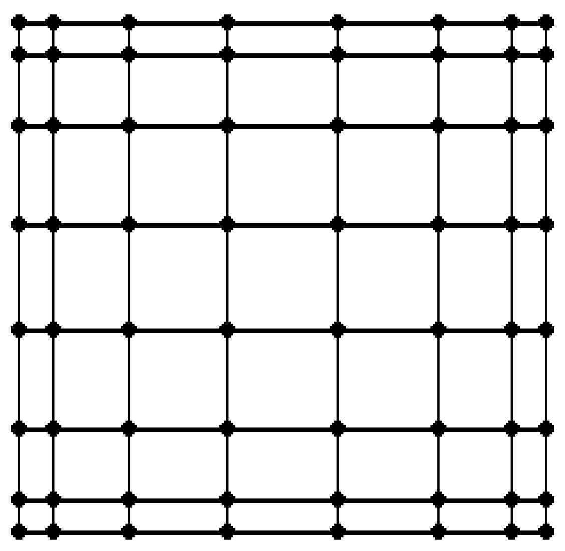
Spatial discretization employs Gauss–Lobatto–Legendre (GLL) points within each element (Figure 2). Time integration in NEKO combines implicit and explicit schemes. Viscous diffusion terms are treated implicitly using backward differentiation formulas (BDF), while the nonlinear advection terms are handled explicitly using Adams–Bashforth or extrapolation schemes, depending on the selected BDF order. NEKO employs the $P_N$–$P_N$ splitting methodology proposed by Karniadakis [24]. Unlike the classical $P_N$–$P_{N-2}$ approach introduced by Maday and Patera [25], which solves pressure on Gauss–Legendre points without boundary nodes, the $P_N$–$P_N$ formulation solves both pressure and velocity on the same GLL points. This avoids compatibility issues between function spaces and enables the use of a uniform polynomial degree for all solution variables [15]. However, the equal-order formulation also increases the computational cost of the pressure solve, as it results in a larger pressure system than the $P_N$–$P_{N-2}$ formulation. In NEKO, this additional cost is partly offset by its matrix-free operator evaluation and projection-based initial guesses, which keep the larger pressure solve tractable.

3. Computational Setup

This section outlines the computational methodology adopted for the numerical simulations performed using the high-order spectral element CFD solver NEKO. At the time of this study, NEKO version 0.9.2 was used. A newer major release, NEKO v1, is currently available on the NEKO Git repository and includes some additional features not considered in the present work.

A well-documented airfoil with available experimental data is required for solver validation. The Eppler 387 (E387) airfoil is selected for this purpose. Experimental data for this airfoil, including lift, drag, and surface pressure distributions, are taken from the study conducted in 1988 by McGhee, Walker, and Millard at the NASA Langley Research Center, and published as NASA Technical Memorandum 4062 [27]. Additionally, information regarding laminar separation, transition to turbulence, and turbulent reattachment characteristics was obtained from the study by [28]. This reference was used as a benchmark for validating the predicted flow features and characteristic locations observed in the present simulation.

The angle of attack was set to 4° with a polynomial order of 3 used for all NEKO simulations. A Reynolds number of ${10}^5$ is employed, as it allows faster turnaround with reduced computational cost while providing sufficient insight into grid resolution requirements and mesh-independence behavior. During mesh sensitivity study, smaller computational domains and relatively larger wall-normal non-dimensional distances ($y^{+}$) were considered. Study emphasized the importance of a sufficiently large domain to reduce boundary-induced artifacts and improved accuracy of aerodynamic coefficients, particularly lift. This process provides a broader understanding of the required numerical parameters and computational cost associated with key bottlenecks such as, high-order wall-resolved LES, and the absence of adaptive mesh refinement (AMR) and wall models. WR-LES resolves the near-wall flow in a manner similar to Direct Numerical Simulation (DNS), which significantly increases computational cost due to the fine resolution required in the boundary layer. In addition, the NEKO version used in this study does not support LES execution on GPUs, nor does it provide regional p-refinement or wall models for curved geometries. Consequently, increasing the polynomial order leads to a global increase in the number of Gauss–Lobatto–Legendre (GLL) points, resulting in an exponential growth in the total degrees of freedom (DOFs). In SEM, the total number of spectral collocation points in three dimensions can be approximated as

$$\mathrm{Total}\mathrm{collocation}\mathrm{points}\approx \left(\mathrm{Number}\mathrm{of}3\mathrm{D}\mathrm{elements}\right)\times {(N+1)}^3,$$

where $(N+1)$ represents the number of collocation points in each spatial direction within an element. Simulations involving several million collocation points are executed in parallel on HPC systems. All simulations were performed on AMD EPYC 9554 64-core CPU nodes, with 128 CPUs per node and 6 GB RAM per CPU, on the University of Oldenburg HPC cluster.

3.1. Geometry and Domain

The airfoil coordinates were obtained from the UIUC Airfoil Coordinate Database in .dat format [29] and subsequently converted into .msh, .re2, and .nmsh formats by using Gmsh, Nek5000, and NEKO, respectively. The coordinates were already normalized, providing a chord length of unity. The airfoil has a maximum thickness of 0.09 at 31% of the chord length and a maximum camber of 0.037 at 40% of the chord.

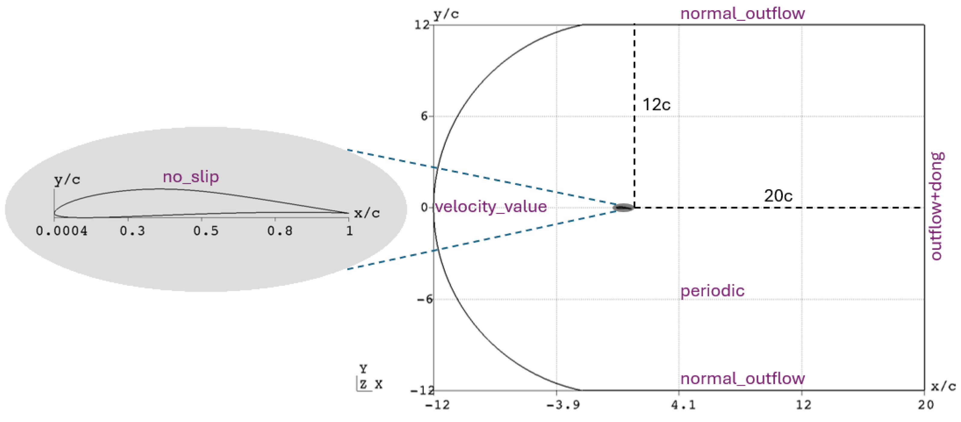
Figure 3 shows the airfoil within the computational domain along with the boundary conditions used. A 3 dimensional semi-circular C-shaped domain was employed for the simulation. This configuration allows downstream elements to be arranged in a structured manner and ensures high-resolution capture of vortex shedding and wake features. The downstream boundary is located 20 chord lengths from the airfoil, while the far-field boundaries and upstream boundary are placed 12 chord lengths away, providing a sufficiently large flow domain to minimize boundary effects.

After smoothing in Nek5000, the mesh was extruded to create six layers along the span of the airfoil. These layers correspond to 19 GLL nodes distributed along a span length of 0.1 m (10% of the chord), yielding a $z^{+}$ value near 45. These dimensions are consistent with high-fidelity DNS and WR-LES studies. Hosseini [30] used domain limits of 1c upstream, 5c downstream, 1c vertically on either side, and a spanwise extent of 0.1c for DNS at Re = 4 × ${10}^5$, while Vinuesa [31] recommended a minimum vertical domain size of 4c. For WR-LES of NACA 4412 at Re = $1.64\times {10}^6$, Frere et al.[3] showed that a 1% wall-resolved mesh produces results within 6–7% of experimental data. Kaltenbach and Choi [32] reported negligible influence of span variation between 2.5% and 5%, concluding that $z^{+}=15$–20 and $x^{+}\approx 60$ are sufficient to resolve near-wall structures.

3.2. Computational Mesh

A mesh-sensitivity study was carried out to assess the dependence of the predicted aerodynamic coefficients on grid resolution. Three grids, M1, M2, and M3, were considered, obtained by successively refining the wall-normal spacing such that the first collocation-point distance from the wall decreased from $y^{+}\approx 0.77$ (M1) to $y^{+}\approx 0.14$ (M3), with the total number of GLL points increasing correspondingly from 8.2 to 42.7 million (

Table 1. Mesh-sensitivity study for the NEKO WR-LES: lift and drag coefficients for three grids of increasing near-wall resolution, from M1 to M3, with the corresponding number of GLL points. The experimental reference values are $C_l=0.778$ and $C_d=0.023$ [27].

MESH	M1 (y+ 0.77)	M2 (y+ 0.37)	M3 (y+ 0.14)
GLL nodes	8.2 million	19.2 million	42.7 million
$C_l$	0.721	0.774	0.767
$C_d$	0.039	0.030	0.030

). The lift coefficient increases markedly from M1 to M2, after which it changes by only approximately 0.9% on the finest grid, M3, indicating that the lift prediction is relatively insensitive to further refinement beyond M2. The drag coefficient decreases from M1 to M2 and remains unchanged on M3, showing a similar convergence behaviour. On this basis, M2 was selected for the production simulations as the best compromise between accuracy and computational cost, since further refinement to M3 doubles the number of GLL points while producing only a negligible change in the aerodynamic coefficients.

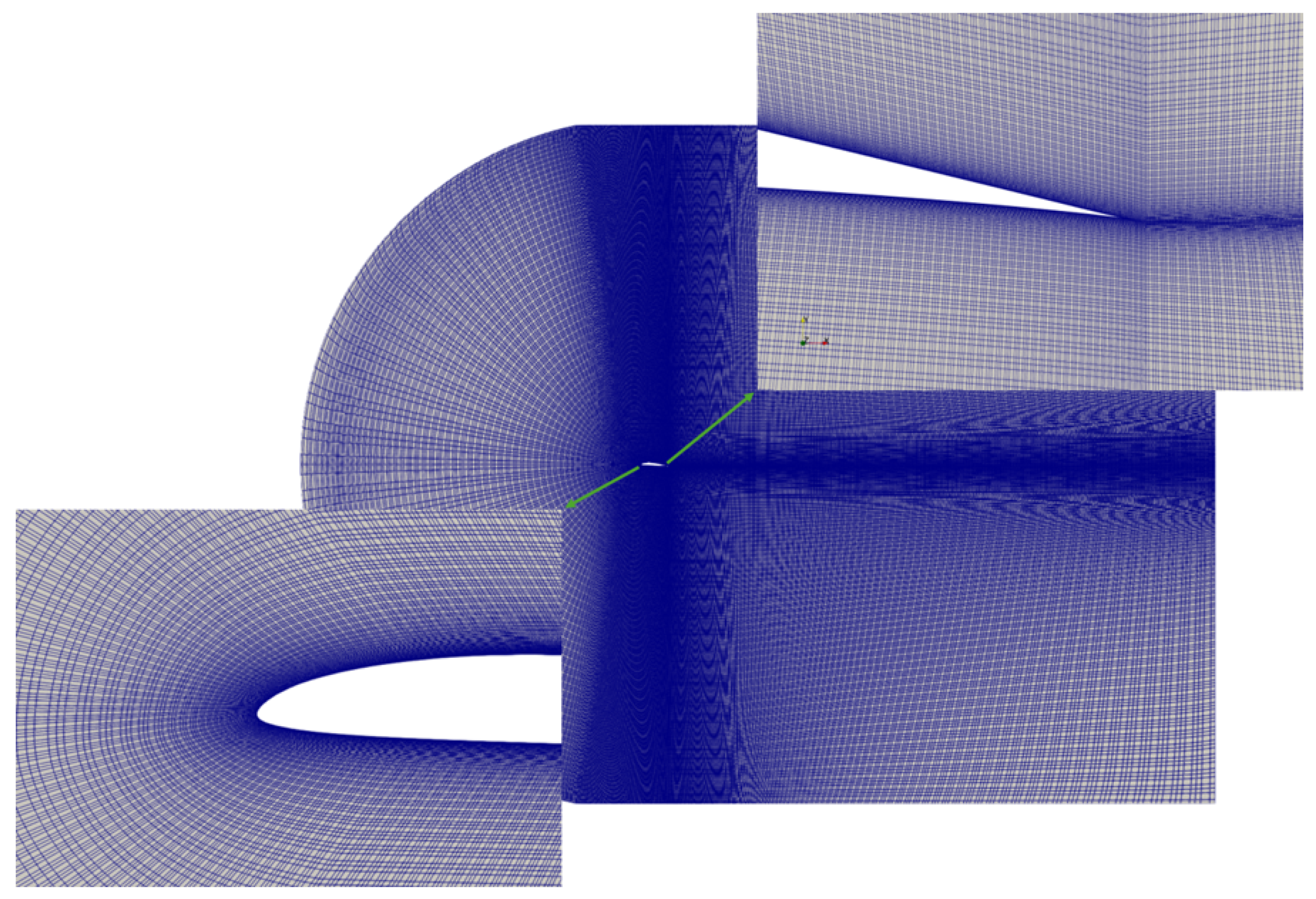
The mesh (Figure 4) was designed to satisfy wall-resolved LES requirements while ensuring high element quality. The first SEM element lies at a $y^{+}$ distance of 1.37, while the first collocation point is located at $y^{+}=0.37$, which represents the actual wall-unit distance used in the simulation. This demonstrates a key advantage of SEM, where wall-resolution requirements are met through collocation-point placement rather than the element size itself. Elements expand in the wall-normal direction using a growth ratio. The $x^{+}$ values are maintained below 5 in critical regions and below 35 elsewhere. Along the airfoil surface, 110 elements with polynomial order 3 yield 331 GLL nodes, ensuring good resolution of velocity and pressure fields.

Mesh generation was performed using Gmsh [33] with a programmable .geo file, which will facilitate the easy modification of mesh parameters. The multi-block design enables h-type refinement in critical regions with strong adverse gradients, and the wake, while allowing coarser resolution in the far-field. Two mesh-generation approaches were considered. The first involves directly creating a 3D mesh in Gmsh. The second approach employs Nek5000 to smooth and extrude a 2D mesh, improving element quality and nodal positions, which reduces the pressure-iteration cost.

The airfoil .dat file was converted to .geo format using a Python (v3.10.12) script. Two .msh files were then generated in Gmsh. A 2D mesh (version 2 binary, second-order elements) was imported into Nek5000 for smoothing and subsequent extrusion to obtain the final 3D mesh used in NEKO. In parallel, a 3D mesh (version 2 ASCII, first-order elements) was exported to OpenFOAM [34] for mesh quality assessment, as NEKO and Nek5000 currently lack dedicated mesh quality evaluation tools. It should be noted that the smoothed, second-order mesh produced by Nek5000 inherently exhibits higher element quality than what is reflected in the OpenFOAM-based checks. The mesh quality assessment indicated acceptable overall mesh characteristics, with low skewness (maximum value of 3.02), moderate non-orthogonality (average of $19.9°$), positive interpolation and volume ratio metrics. Although a few cells were flagged with low determinant values, these represent only a small fraction of the total mesh and are expected to have negligible influence on the solution accuracy after the subsequent smoothing procedure in Nek5000.

Mesh smoothing was performed in Nek5000 using the algorithm by Mittal and Fischer [35], combining Laplacian smoothing with optimization based on the Jacobian condition number [36]. The smoothmesh function adjusts node positions to minimize geometric distortions, preserve boundary layers, and maintain smooth transitions between elements. The 2D mesh was smoothed, extruded into 3D, and exported as a .re2 file, which was converted to .nmsh using NEKO’s rea2nbin utility. Periodic boundary information were preserved within the mesh here. The final mesh was selected based on a mesh independence study, in which the computational domain was progressively enlarged and the wall-normal resolution parameter ($y^{+}$) was reduced. These refinements led to a noticeable improvement in predictive accuracy, particularly for the lift coefficient.

3.3. NEKO Simulation Setup

NEKO simulations require a .nmsh mesh file and a .case file, which defines all simulation parameters. Optionally, a user-defined FORTRAN file (.f90) can be included to implement custom functions or modules, extending the functionality of the NEKO executable. Due to the high cost of WR-LES, simulations were executed on HPC clusters [37] using a SLURM sbatch script. The .case file [38], written in JSON format, specifies solver settings, polynomial and time orders, Reynolds number, inflow, initial & boundary conditions, convergence limits, solvers, preconditioners, and output frequencies. Checkpoints allow simulations to stop or restart at specified intervals. Projection spaces can be used to accelerate convergence. When only Reynolds number is specified, density is assumed to be 1 kg/m³ and viscosity is computed as $\mu =1/\mathrm{Re}$ as part of non-dimensionalisation in NEKO.

Simulations were run with a target CFL of $0.7\pm 0.1$, variable timestep, and a maximum timestep limit. Pressure converged within 50 iterations per timestep, indicating good numerical stability. Polynomial and time orders were both set to 3, with PnPn discretization at Re = ${10}^5$ and AOA = 4°. PnPn refers to the polynomial order used for both velocity and pressure fields being the same. Velocity and pressure solvers were coupled_cg and gmres, with Jacobi and HSMG preconditioners. Convergence criteria were $1.0\times {10}^{-7}$ for velocity and $1.0\times {10}^{-5}$ for pressure, with a maximum of 800 iterations. Uniform inflow velocity $(1,0,0)$ was prescribed at inlet. A zero-pressure outlet with the energy-stable outflow condition of Dong et al. [39] was applied. This DONG condition suppresses the uncontrolled influx of kinetic energy that can occur at outflow boundaries on severely truncated domains, preventing backflow-driven instabilities without a mesh sponge. Strong numerical oscillations can trigger instabilities. No-slip condition was imposed on the airfoil surface, normal outflow on top and bottom boundaries (Dirichlet for velocity parallel to the wall and homogeneous Neumann for the wall-normal component allowing disturbances to exit the domain smoothly), and periodic conditions in the spanwise direction. Boundary conditions were verified using bdry0.fld file.

NEKO’s simulation_components enabled computation of ${\lambda }_2$ fields (a standard vortex-identification criterion [40] used to detect and visualise vortex cores in the flow), aerodynamic forces, SGS models, and fluid statistics. It also assists in writing multiple SGS fields within the same simulation to compare turbulent viscosity fields. Turbulence statistics were written to stats0.f00000 and post-processed using NEKO utilities like scripts that average the fields in time and along the spanwise direction to obtain the mean quantities. The 2D mesh contained 50,160 elements, increasing to 300,960 elements after extrusion. With polynomial order 3, approximately 19 million collocation points were used. The simulation used 256 cores, distributed over two AMD EPYC 9554 64-core dual-socket nodes using the STORM partition, and ran for approximately 103 h.

3.4. OpenFOAM 2D RANS Simulation Setup

Validation against an established numerical solver like OpenFOAM provides a benchmark for the NEKO simulations. Two-dimensional steady-state simulations were performed using OpenFOAM solver - simpleFoam with three different RANS models: the k–$\omega$ Shear Stress Transport (KOSST) model, the k–$\omega$ SST Langtry–Menter (KOSSTLM) model, and the KOSSTCND model, which is the standard SST model augmented with a correction term for separated flows derived from machine learning.

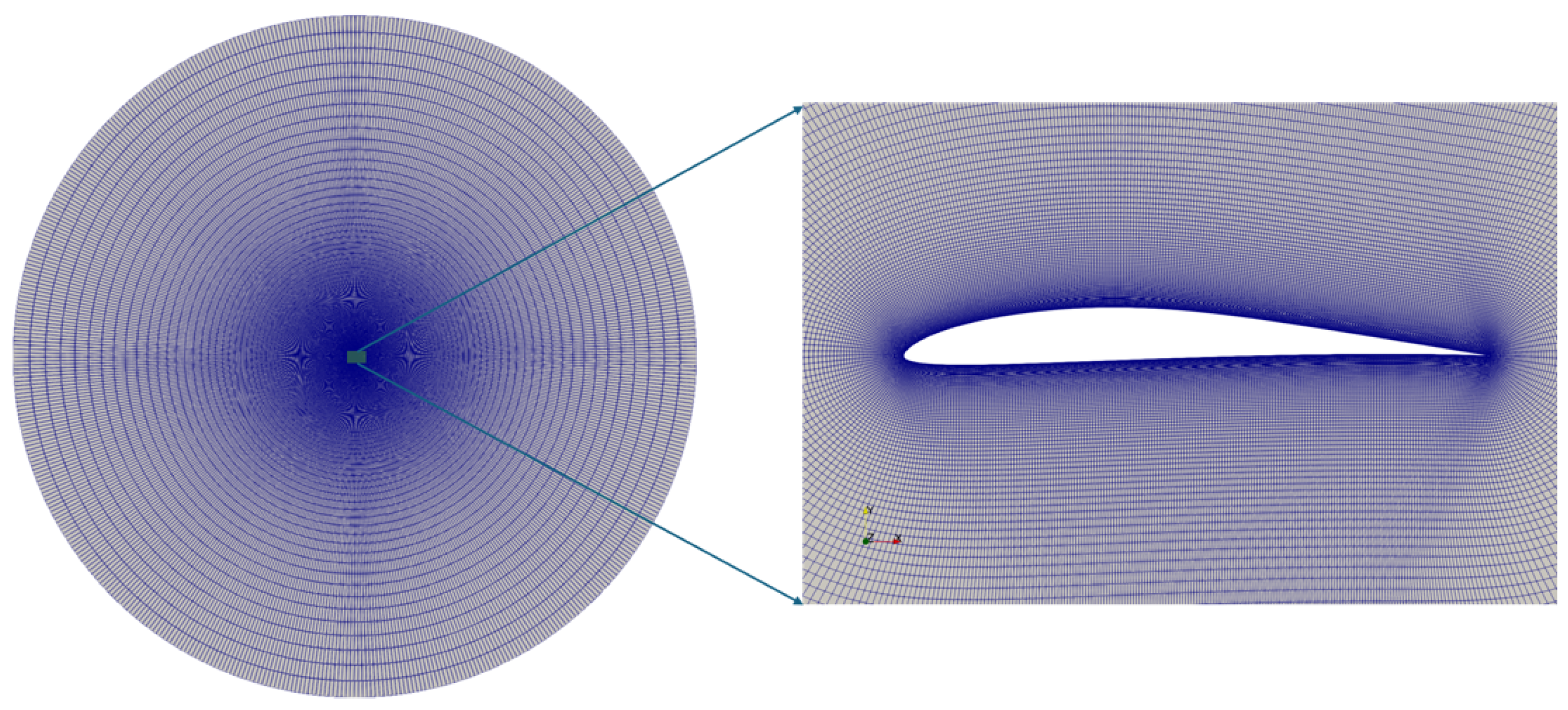
A 2D O-type mesh (Figure 5) with a radius of 300 chord lengths was used, providing sufficient domain size upstream, downstream, and in the far-field, effectively eliminating boundary effects on the airfoil surface. The total number of cells in the mesh was 130,580, with a $y^{+}$ value of 0.5 to accurately resolve the near-wall flow. Simulations employed a maximum CFL number of 0.2, with adaptive timesteps, and outputs were written with a precision of 16 digits. Numerical tolerances were set very low, with iterative solvers converging to $1\times {10}^{-10}$, ensuring high numerical accuracy in particular.

4. Results

To validate the numerical methodology, the aerodynamic force coefficients and the pressure distribution across the chord are compared with experimental results (Section 4.1). Although the reference experiment investigated multiple Reynolds numbers and angles of attack, the present numerical setup focuses on a Reynolds number of ${10}^5$ and an angle of attack of 4°. Unless stated otherwise, the NEKO quantities reported here are averaged both temporally over the converged interval and spatially along the spanwise direction; instantaneous quantities are explicitly labelled. Flow-field data were recorded at intervals throughout the 70 s simulation, and only the data obtained after convergence, were used for post-processing to extract the lift and drag forces and evaluate the pressure distribution along the airfoil. The NEKO solver computed aerodynamic forces on the airfoil surface, which were subsequently used to calculate the lift and drag coefficients, $C_l$ and $C_d$, plotted against simulation runtime. The planform area, defined as the product of the airfoil span and chord length, which represents the effective surface exposed to the incoming flow that contributes to lift and drag generation was used as the reference area for the calculations.

4.1. Force Coefficients and Pressure Distribution

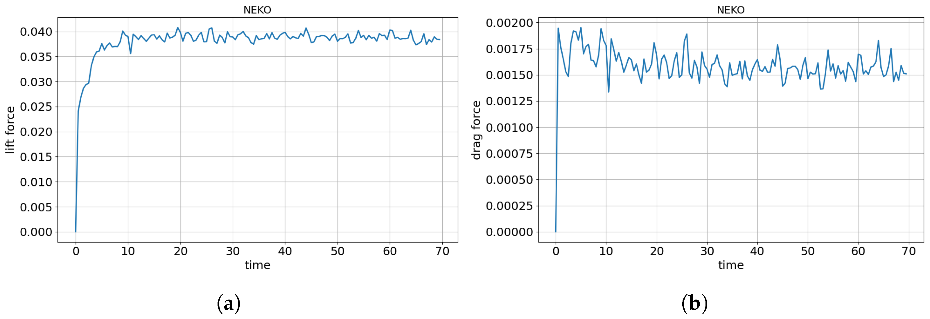
Figure 6 shows the time histories of the lift and drag forces. After an initial transient, both signals reach a statistically stationary state, fluctuating about a constant mean. Statistics were accumulated over 40–70 s to calculate the lift and drag coefficients. The running means plateau well within this interval, which spans multiple shedding cycles and confirms statistical convergence. The experimental lift coefficient ($C_l$) was 0.778, while NEKO predicted 0.774, resulting in a very small error of 0.51%. In contrast, the experimental drag coefficient ($C_d$) was 0.023, whereas NEKO yielded 0.030, a significant deviation.

Table 2. Comparison of experimental [27] and NEKO simulation results against OpenFOAM RANS models for lift and drag coefficients ($C_l$ and $C_d$).

Coefficient	Experimental	NEKO	KOSST	KOSSTLM	KOSSTCND
$C_l$	0.778	0.774	0.761	0.755	0.762
$C_d$	0.023	0.030	0.016	0.024	0.018

summarizes the comparison of NEKO results with experimental measurements and OpenFOAM simulations. All three RANS models underpredicted lift, producing lower values than NEKO. Regarding drag, two of the RANS models underestimated the coefficient, while the KOSSTLM model closely matched the experimental value. These results point to the trade-off between RANS models: a model that predicts lift more accurately is underpredicting drag, and vice versa in the case. For NEKO, even though the mesh independence study significantly improved the approximation for lift coefficient, the drag coefficient remains overpredicted, indicating further refinement—potentially in spanwise resolution or span length could enhance more agreement with experimental data. But this refinement will significantly increase the total GLL nodes making such simulation prohibitively expensive.

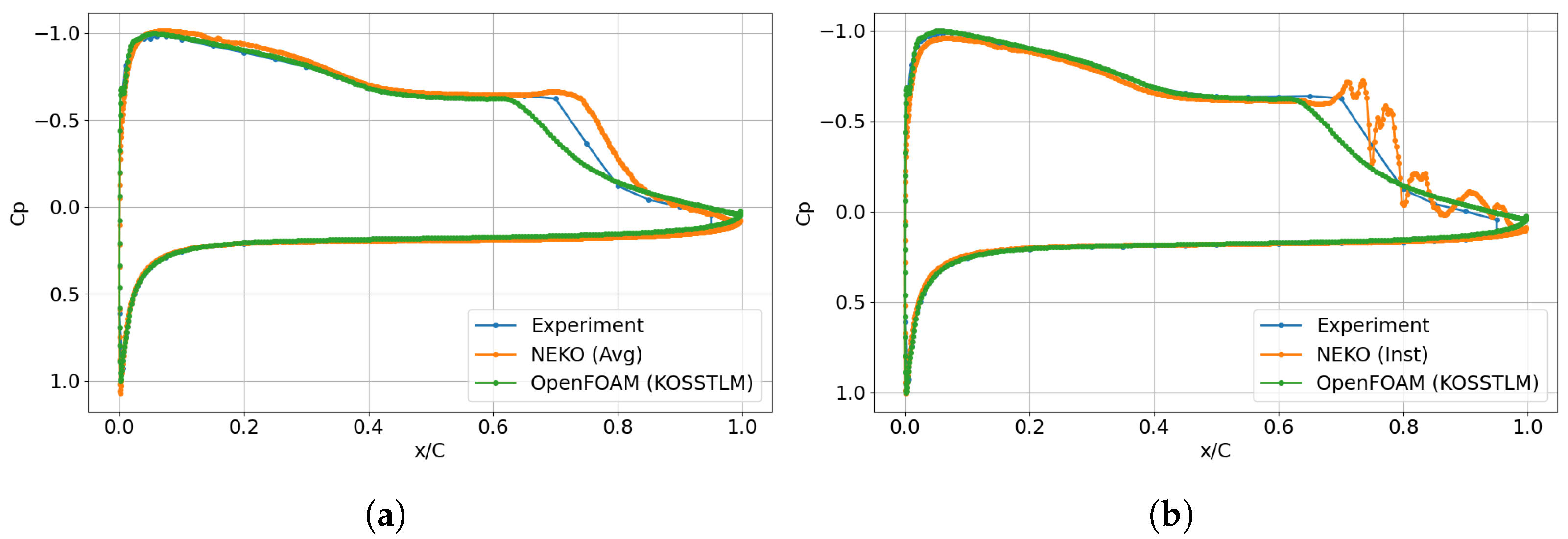
The flow fields obtained after the initial transients had decayed were extracted and time-averaged to obtain the temporal mean, thereby minimizing the influence of extreme oscillations in the transition region on the pressure coefficient ($C_p$). Figure 7a describes the pressure distribution coefficient, which was calculated using free-stream pressure as reference and plotted along the normalized chord length. The y-axis is inverted to follow standard airfoil conventions, with negative values indicating suction on the upper surface and positive values representing higher pressure on the lower surface. NEKO results (orange dotted line) show excellent agreement with experimental data (blue dotted line), comparable to OpenFOAM simulation KOSSTLM (green dotted line). Both solvers exhibit deviations in the transition region around $x/c\approx 0.7$. NEKO predicts the transition point farther downstream whereas OpenFOAM predicts it earlier compared to the experimental data. Despite these discrepancies, both solvers converge to similar pressure values near the trailing edge. Overall, the numerical solvers capture the experimental pressure distribution well over most of the chord, illustrating the challenges of accurately modeling laminar–turbulent transition and separation even with high-fidelity CFD. It is important to note that the NEKO time-averaged pressure distribution may carry a small error due to a bug in the average_fields_in_time utility at the time, which required post-normalization of fields. To verify this, instantaneous pressure distributions were examined (Figure 7b), showing excellent agreement with experimental data in the transition region, capturing the transition point and region more accurately. The oscillations downstream of the transition in instantaneous plots are associated with regime changes and localized pressure pockets from vortex shedding. A proper time-averaged representation would smooth these oscillations.

NEKO predicts lift coefficient accurately, showing only a 0.004 deviation from experiments, while drag is overpredicted. The drag discrepancy is likely linked to limited spanwise resolution. Another contributing factor is the absence of inflow turbulence in the simulation, unlike the wind tunnel experiment. The free-transition setup, without any turbulence inflow or generators, likely shifted the flow separation to the trailing edge, contributing to drag overprediction as well. Nevertheless, the close match in pressure distributions confirms that the solver captures the essential flow physics reliably. Further refinement of spanwise resolution and inflow conditions is expected to improve drag prediction.

4.2. Flow Fields

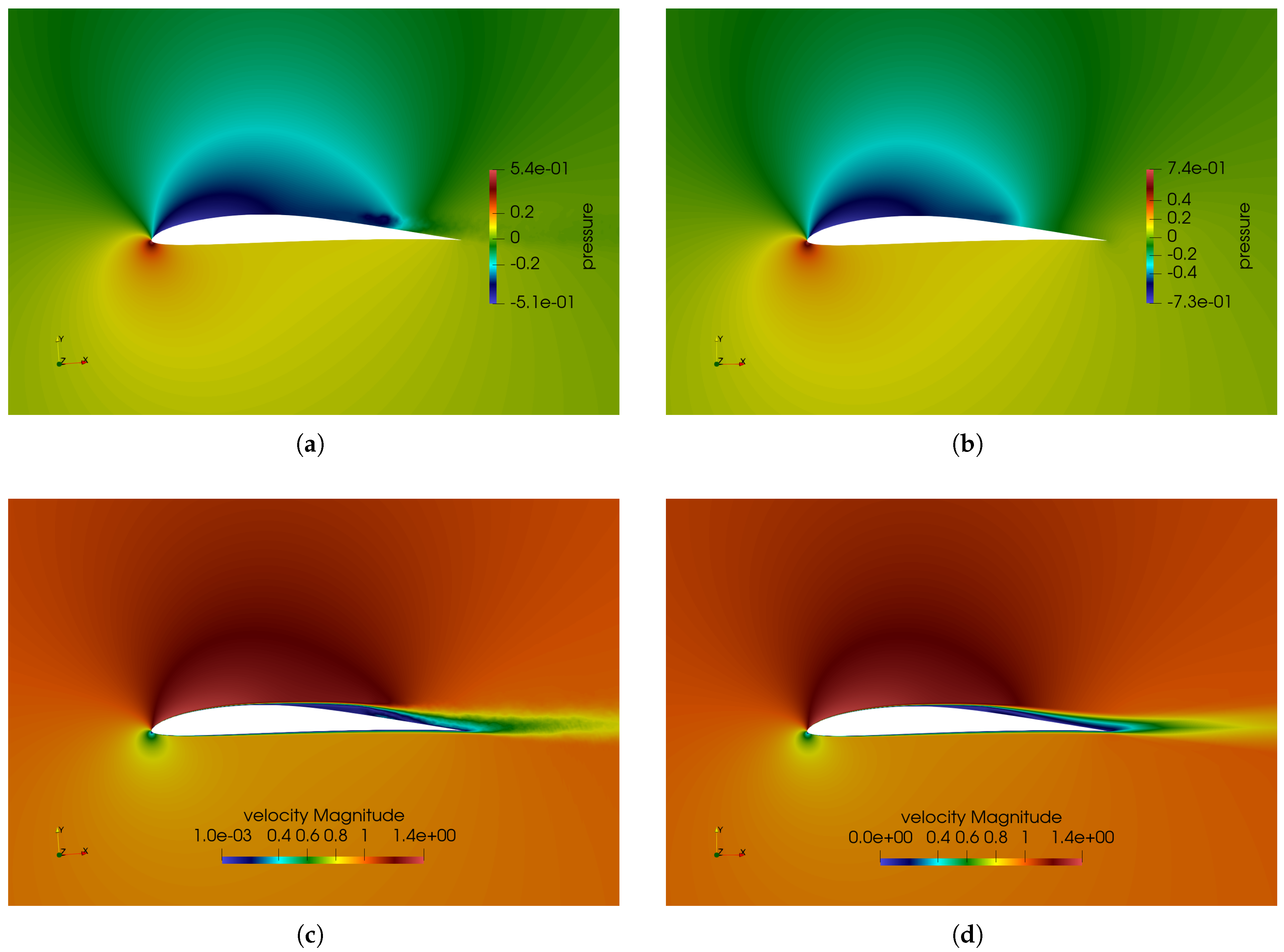
Figure 8, instantaneous flow fields from NEKO simulation provide a detailed picture of the aerodynamic behavior around the Eppler 387 airfoil. The velocity field reveals vortex shedding originating from the separated flow region following the collapse of the laminar separation bubble. Once separation occurs, the flow transitions to turbulence, generating unsteady vortices which arise from the instabilities in the separated shear layers. After separation, turbulent reattachment occurs on the suction side of the airfoil at aft chord, while the pressure side remains largely attached, exhibiting only a thin boundary layer. The polynomial order of 3 used in the NEKO simulation allows fine resolution of flow structures, capturing detailed features of the fields. The Sigma subgrid-scale (SGS) model regulates turbulent viscosity, influencing near-wall effects. Downstream of the separation, vortices weaken gradually broadening the wake and dissipating energy within the extended computational domain. Initial strong eddies induced numerical instabilities near the outlet, mitigated by the DONG outlet condition which prevented backflow and thereby improved numerical stability. The absence of distinct low-pressure regions further downstream suggests enhanced turbulent mixing and smaller, less coherent structures in the wake.

Comparison with OpenFOAM fields shows that the flow fields exhibit strong qualitative agreement, despite the fundamental differences in modeling approaches—RANS for OpenFOAM and LES for NEKO. To enable a like-for-like comparison, both datasets are considered as mean fields. The steady 2D RANS solution represents the Reynolds-averaged flow and is invariant in the spanwise direction, whereas the NEKO mean fields are obtained by averaging the unsteady three-dimensional LES both in time and along the spanwise direction. Thus, both datasets represent statistically two-dimensional, time- and spanwise-averaged mean fields.

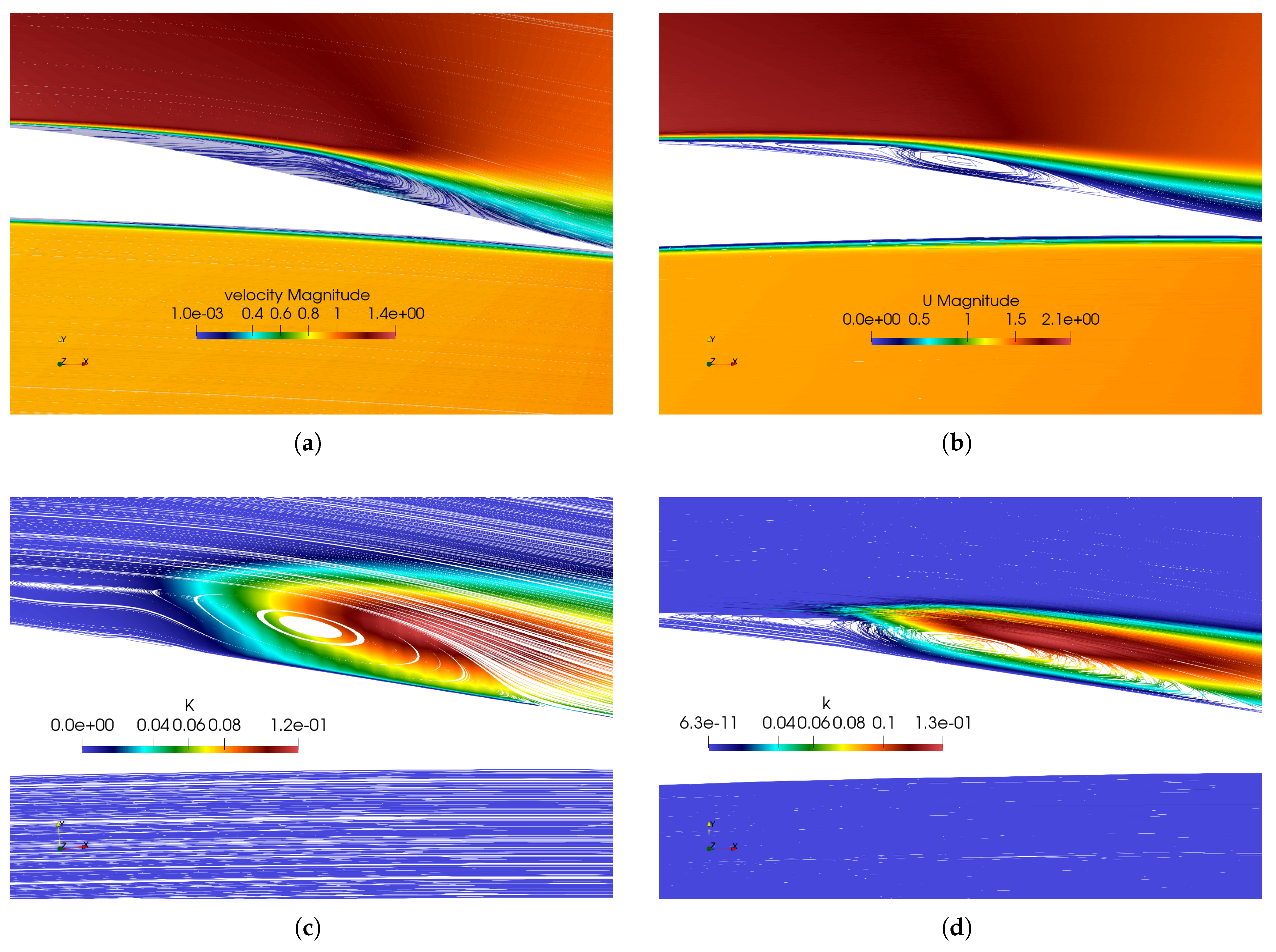
The stream tracers from both solvers exhibit similar flow topology, with comparable separation, transition, and reattachment regions, as shown in Figure 9. This quantitative comparison is summarized in

Table 3. Comparison of experimental [28] and NEKO results against OpenFOAM results for separation, transition and turbulent reattachment locations.

	Separation (x/c)	Transition (x/c)	Reattachment (x/c)
Experiment	0.386	0.694	0.795
NEKO	0.38	0.68	0.83
OpenFOAM	0.40	0.65	0.80

. A distinct stagnation point is observed near the leading edge on the pressure-side lower surface. NEKO and OpenFOAM predict the stagnation point at similar locations, with positions of 0.0016c and 0.0019c, respectively. The deviation of 0.0003c between the two predictions is negligible relative to the chord length. The experimental measurements of the separation point, recirculation region, transition onset, and reattachment location reported in [28] provide a reference for validating the simulation results. The predicted flow characteristics are consistent with the experimental observations for the airfoil at low Reynolds number. Compared with the literature values, NEKO predicts these characteristic flow locations more accurately than OpenFOAM. The approximate transition location in the OpenFOAM RANS solution was estimated from the distribution of turbulent kinetic energy (TKE). NEKO predicts slightly larger separation region (~45%c) with more abrupt reattachment, whereas OpenFOAM (~40%c) exhibits a gradual reattachment. The resolved turbulent kinetic energy from NEKO is compared with the modelled TKE from RANS in Figure 9c,d. The two fields show partial agreement in the region and the match is less tight than for the mean fields, as expected for second-order statistics. The resolved-versus-modelled distinction accounts for part of the difference. Note that the RANS field is fully modelled whereas the LES field is the resolved contribution; the subgrid part is small in this wall-resolved setup. Differences in inflow conditions between the solvers were accounted for by scaling the OpenFOAM fields for fair comparisons.

5. Conclusions

This study demonstrated the capability of the Spectral Element Method solver NEKO to perform wall-resolved large-eddy simulations of the Eppler 387 airfoil at a low Reynolds number of ${10}^5$. SEM offers advantages over traditional low-order numerical methods, including higher polynomial and temporal orders, spectral accuracy, and reduced numerical dispersion and dissipation. Despite the inherent challenges associated with WR-LES—particularly the high computational cost and the absence of region-based mesh refinement—the simulations successfully captured key aerodynamic features. Comparisons with experimental data and OpenFOAM RANS models showed that NEKO predicts lift and separation accurately and reproduces pressure and velocity flow fields in strong qualitative agreement with simpleFoam solver. While drag was overpredicted and transition was not fully captured compared to the experiment, these discrepancies are attributed to the absence of inflow turbulence from the wind tunnel and limitations in spanwise resolution, both of which were consistently reflected across the flow-field and coefficient analyses. In a nutshell, while the current NEKO results may not be fully optimal, the solver paves a promising new path in CFD through SEM, offering significant potential. It is important to note that NEKO and OpenFOAM differ fundamentally in their numerical approaches—SEM-based LES for NEKO and FVM RANS for OpenFOAM—as well as in the computational setups employed, including convergence criteria, maximum CFL, inflow conditions, $y^{+}$ values, spanwise resolution, and domain size. The results highlight the strength of SEM in resolving fine-scale unsteady structures using high-order polynomial discretization, even with comparatively coarser meshes enabled by Gauss–Lobatto–Legendre nodal distribution. Although NEKO provides promising results, the computational expense from the absence of adaptive mesh refinement and wall models presently make it practically unreasonable. By harnessing the spectral accuracy of the Spectral Method and the geometric flexibility of the Finite Element Method, the Spectral Element Method (SEM) offers immense potential for advancing CFD research.

References

1. Abbott, I.H.; von Doenhoff, A.E.; Stivers, L., Jr. Summary of Airfoil Data from Tests in the Langley Two-Dimensional Low-Turbulence Pressure Tunnel; NACA Technical Report 824; National Advisory Committee for Aeronautics: Langley Field, VA, USA, 1945.
2. Scotto di Perta, E.; Agizza, M.A.; Sorrentino, G.; Boccia, L.; Pindozzi, S. Study of aerodynamic performances of different wind tunnel configurations and air inlet velocities, using computational fluid dynamics (CFD). Comput. Electron. Agric. 2016, 125, 137–148. [Google Scholar] [CrossRef] [Scilit]
3. Frère, A.; Hillewaert, K.; Chatelain, P.; Winckelmans, G. High Reynolds Number Airfoil: From Wall-Resolved to Wall-Modeled LES. Flow Turbul. Combust. 2018, 101, 457–476. [Google Scholar] [CrossRef] [Scilit]
4. Lusher, D.J.; Zauner, M.; Sansica, A.; Hashimoto, A. Automatic Code-Generation to Enable High-Fidelity Simulations of Multi-Block Airfoils on GPUs. In Proceedings of the AIAA Scitech 2023 Forum 2023, National Harbor, MD, USA, 23–27 January 2023. [Google Scholar]
5. Kroll, N.; Leicht, T.; Hirsch, C.; Bass, F.; Johnston, C.; Sørensen, K.A.; Hillewaert, K. Results and Conclusions of the European Project IDIHOM on High-Order Methods for Industrial Aerodynamic Applications. In Proceedings of the 53rd AIAA Aerospace Sciences Meeting, Kissimmee, FL, USA, 5–9 January 2015. [Google Scholar]
6. Gross, A.; Marks, C.; Sondergaard, R. Laminar Separation Control for Eppler 387 Airfoil Based on Resolvent Analysis. AIAA J. 2024, 62, 1487–1502. [Google Scholar] [CrossRef] [Scilit]
7. Catalano, P.; de Rosa, D. Large Eddy Simulations and RANS Models for Airfoils at Low Reynolds Number. In AIAA AVIATION 2020 Forum; AIAA Paper 2020–2990; American Institute of Aeronautics and Astronautics: Reston, VA, USA, 2020. [Google Scholar]
8. Beck, A.D.; Bolemann, T.; Flad, D.; Frank, H.; Gassner, G.J.; Hindenlang, F.; Munz, C.-D. High-Order Discontinuous Galerkin Spectral Element Methods for Transitional and Turbulent Flow Simulations. Int. J. Numer. Methods Fluids 2014, 76, 522–548. [Google Scholar] [CrossRef] [Scilit]
9. Tonicello, N.; Lodato, G.; Vervisch, L. Analysis of High-Order Explicit LES Dynamic Modeling Applied to Airfoil Flows. Flow Turbul. Combust. 2022, 108, 77–104. [Google Scholar] [CrossRef] [Scilit]
10. Garmann, D.J.; Visbal, M.R.; Orkwis, P.D. Comparative Study of Implicit and Subgrid-Scale Model Large-Eddy Simulation Techniques for Low-Reynolds Number Airfoil Applications. Int. J. Numer. Methods Fluids 2013, 71, 1546–1565. [Google Scholar] [CrossRef] [Scilit]
11. Capuano, F.; Beratlis, N.; Zhang, F.; Peet, Y.; Squires, K.; Balaras, E. Cost vs Accuracy: DNS of Turbulent Flow over a Sphere Using Structured Immersed-Boundary, Unstructured Finite-Volume, and Spectral-Element Methods. Eur. J. Mech. B/Fluids 2023, 102, 91–102. [Google Scholar] [CrossRef] [Scilit]
12. Buscariolo, F.F.; Hoessler, J.; Moxey, D.; Jassim, A.; Gouder, K.; Basley, J.; Murai, Y.; Assi, G.R.; Sherwin, S.J. Spectral/HP Element Simulation of Flow Past a Formula One Front Wing: Validation Against Experiments. J. Wind Eng. Ind. Aerodyn. 2022, 221, 104832. [Google Scholar] [CrossRef] [Scilit]
13. Xu, H.; Cantwell, C.D.; Monteserin, C.; Eskilsson, C.; Engsig-Karup, A.P.; Sherwin, S.J. Spectral/HP Element Methods: Recent Developments, Applications, and Perspectives. J. Hydrodyn. 2018, 30, 1–22. [Google Scholar] [CrossRef] [Scilit]
14. Choi, J.J. Hybrid Spectral Difference/Embedded Finite Volume Method for Conservation Laws. J. Comput. Phys. 2015, 295, 285–306. [Google Scholar] [CrossRef] [Scilit]
15. Karp, M.; Massaro, D.; Jansson, N.; Hart, A.; Wahlgren, J.; Schlatter, P.; Markidis, S. Large-Scale Direct Numerical Simulations of Turbulence Using GPUs and Modern Fortran. Int. J. High Perform. Comput. Appl. 2023, 37, 487–502, Erratum in Int. J. High Perform. Comput. Appl. 2025, 39, 477. [Google Scholar] [CrossRef] [Scilit]
16. Kim, B.H. A Graphical Preprocessing Interface for Non-Conforming Spectral Element Solvers; Technical Report; Texas A&M University: College Station, TX, USA, 2006. [Google Scholar]
17. Jansson, N.; Karp, M.; Podobas, A.; Markidis, S.; Schlatter, P. Neko: A modern, portable, and scalable framework for high-fidelity computational fluid dynamics. Comput. Fluids 2024, 275, 106243. [Google Scholar] [CrossRef] [Scilit]
18. Pope, S.B. Turbulent Flows; Cambridge University Press: Cambridge, UK, 2000. [Google Scholar]
19. Leonard, A. Energy cascade in large-eddy simulations of turbulent fluid flows. Adv. Geophys. 1975, 18, 237–248. [Google Scholar] [CrossRef] [Scilit]
20. Nicoud, F.; Toda, H.B.; Cabrit, O.; Bose, S.; Lee, J. Using Singular Values to Build a Subgrid-Scale Model for Large Eddy Simulations. Phys. Fluids 2011, 23, 085106. [Google Scholar] [CrossRef] [Scilit]
21. Sagaut, P. Large Eddy Simulation for Incompressible Flows: An Introduction, 3rd ed.; Springer: Berlin/Heidelberg, Germany, 2006. [Google Scholar]
22. Mukha, T.; Parsani, M.; Schlatter, P. Wall-Modeled Large-Eddy Simulation Based on Spectral-Element Discretization. Phys. Fluids 2025, 37, 105158. [Google Scholar] [CrossRef] [Scilit]
23. Fischer, P.F. Projection Techniques for Iterative Solution of Ax=b with Successive Right-Hand Sides. Comput. Methods Appl. Mech. Eng. 1998, 163, 193–204. [Google Scholar] [CrossRef] [Scilit]
24. Karniadakis, G.E.; Israeli, M.; Orszag, S.A. High-Order Splitting Methods for the Incompressible Navier-Stokes Equations. J. Comput. Phys. 1991, 97, 414–443. [Google Scholar] [CrossRef] [Scilit]
25. Maday, Y.; Patera, A.T. Spectral Element Methods for the Incompressible Navier–Stokes Equations. In State-of-the-Art Surveys on Computational Mechanics; Noor, A.K., Oden, J.T., Eds.; ASME: New York, NY, USA, 1989; pp. 71–143. [Google Scholar]
26. Karp, M. Direct Numerical Simulation of Turbulence on Heterogenous Computer Systems: Architectures, Algorithms, and Applications. Ph.D. Thesis, KTH Royal Institute of Technology, Stockholm, Sweden, 2024. [Google Scholar]
27. McGhee, R.J.; Walker, B.S.; Millard, B.F. Experimental Results for the Eppler 387 Airfoil at Low Reynolds Numbers in the Langley Low-Turbulence Pressure Tunnel; NASA TM-4062; National Aeronautics and Space Administration, Langley Research Center: Hampton, VA, USA, 1988.
28. Cole, G.M.; Mueller, T.J. Experimental Measurements of the Laminar Separation Bubble on an Eppler 387 Airfoil at Low Reynolds Numbers; Final Report UNDAS-1419-FR; University of Notre Dame for NASA Langley Research Center: Hampton, VA, USA, 1990. [Google Scholar]
29. Selig, M.S. E387 (e387-il) Airfoil Coordinates. UIUC Airfoil Coordinates Database. Available online: https://m-selig.ae.illinois.edu/ads/coord/e387.dat (accessed on 5 February 2026).
30. Hosseini, S.; Vinuesa, R.; Schlatter, P.; Hanifi, A.; Henningson, D. Direct Numerical Simulation of the Flow Around a Wing Section at Moderate Reynolds Number. Int. J. Heat Fluid Flow 2016, 61, 117–128. [Google Scholar] [CrossRef] [Scilit]
31. Vinuesa, R.; Negi, P.; Hanifi, A.; Henningson, D.; Schlatter, P. High-Fidelity Simulations of the Flow Around Wings at High Reynolds Numbers. In Proceedings of the 10th International Symposium on Turbulence and Shear Flow Phenomena (TSFP), Chicago, IL, USA, 6–9 July 2017. [Google Scholar]
32. Kaltenbach, H.J.; Choi, H. Large-Eddy Simulation of Flow Around an Airfoil on a Structured Mesh; Annual Research Briefs; Center for Turbulence Research, Stanford University: Stanford, CA, USA, 1995. [Google Scholar]
33. Geuzaine, C.; Remacle, J.-F. Gmsh: A three-dimensional finite element mesh generator with built-in pre- and post-processing facilities. Int. J. Numer. Methods Eng. 2009, 79, 1309–1331. [Google Scholar] [CrossRef] [Scilit]
34. OpenFOAM. Available online: https://www.openfoam.com (accessed on 5 February 2026).
35. Mittal, K.; Fischer, P. Mesh smoothing for the spectral element method. J. Sci. Comput. 2019, 78, 1152–1173. [Google Scholar] [CrossRef] [Scilit]
36. Knupp, P. A method for hexahedral mesh shape optimization. Int. J. Numer. Methods Eng. 2003, 58, 319–332. [Google Scholar] [CrossRef] [Scilit]
37. HPC UOL—Carl von Ossietzky Universität Oldenburg. Available online: https://uol.de/fk5/wr/hochleistungsrechnen/hpc-facilities (accessed on 10 September 2026).
38. Neko 1.99.1. Available online: https://neko.readthedocs.io (accessed on 5 February 2026).
39. Dong, S.; Karniadakis, G.E.; Chryssostomidis, C. A Robust and Accurate Outflow Boundary Condition for Incompressible Flow Simulations on Severely-Truncated Unbounded Domains. J. Comput. Phys. 2014, 261, 83–105. [Google Scholar] [CrossRef] [Scilit]
40. Jeong, J.; Hussain, F. On the Identification of a Vortex. J. Fluid Mech. 1995, 285, 69–94. [Google Scholar] [CrossRef] [Scilit]
Figure 1. Spectral element method combining Finite element and Spectral method [16].
Fluids 11 00237 g001
Figure 2. 2D representation of a spectral element with GLL node distribution of order 7 (adapted from [26]).
Fluids 11 00237 g002
Figure 3. Eppler 387 airfoil [29] and computational domain with boundary conditions.
Fluids 11 00237 g003
Figure 4. 2D semi-circular C-shaped computational mesh with close-up view around the airfoil.
Fluids 11 00237 g004
Figure 5. OpenFOAM 2D O-mesh with close-up view around the airfoil.
Fluids 11 00237 g005
Figure 6. Time histories of (a) lift and (b) drag forces from NEKO.
Fluids 11 00237 g006
Figure 7. (a) Averaged NEKO and (b) instantaneous NEKO pressure coefficient (Cp) distribution, comparing against OpenFOAM and experimental data [27].
Fluids 11 00237 g007
Figure 8. Averaged (a) pressure field from NEKO, (b) pressure field from OpenFOAM, (c) velocity field from NEKO, and (d) velocity field from OpenFOAM.
Fluids 11 00237 g008
Figure 9. Streamlines: (a) averaged LES field from NEKO, (b) RANS field from OpenFOAM, (c) resolved turbulent kinetic energy (TKE) from NEKO, and (d) modelled TKE field from OpenFOAM.
Fluids 11 00237 g009