


Abstract
Reliable in-line estimation of slurry rheology could improve the safety and control of pipeline-transfer operations, particularly in radioactive-waste processing where frequent manual sampling is undesirable. This study presents SW-RheoPINN, a physics-informed inverse pipe-rheometry framework for estimating pipe-effective yield stress and plastic viscosity from short windows of pressure-drop, mass-flow-rate, density, and pipe-geometry measurements. The framework combines a permutation-invariant sensor-window encoder with an analytical Bingham pipe-flow backbone, radial momentum balance, a regularized constitutive relation, cross-sectional mass conservation, and a tightly bounded velocity-profile correction for limited model discrepancy. SW-RheoPINN was evaluated using 20 two-state kaolin–water flow-loop experiments comprising 40 hydraulic states. In matched-physics synthetic tests with 2% multiplicative mass-flow noise, yield-stress recovery improved from for two-state windows to and for three- and four-state windows, respectively; plastic-viscosity recovery improved from to and . For the experimental data, complete sensor-window reconstruction achieved a MAPE of 0.80% and . Because measured mass flow is an encoder input in this reconstruction, these metrics characterize inverse self-consistency rather than prospective prediction. A separate target-flow-withheld evaluation, in which the withheld mass flow was not supplied to the inverse model, achieved an RMSE of kg.s-1, , and a median absolute percentage error of 3.55%. Prediction was strongest for compositions with repeatable hydraulic behavior and degraded when nominally similar experiments occupied distinct response states. Ablation and sensitivity analyses showed that strongly resolved high-yield conditions were largely insensitive to composition-related regularization, Papanastasiou sharpness, and correction capacity, whereas low-yield estimates were more model dependent. Misspecified-physics tests further showed that small hydraulic residuals do not necessarily imply unbiased rheological parameters. The inferred pipe-effective yield stresses retained the broad composition-dependent trend observed by offline rheometry, although absolute cross-scale agreement was limited. These results support SW-RheoPINN as a physics-constrained inference and diagnostic framework for identifying both well-supported and weakly resolved rheological states from standard process measurements.
1. Introduction
The safe treatment of legacy nuclear waste depends on the ability to mobilize, mix, and transfer concentrated slurries through process equipment. At the Savannah River Site (SRS), radioactive sludge is retrieved, conditioned, transferred, and prepared as feed for the Defense Waste Processing Facility (DWPF). The hydraulic behavior of these streams is strongly influenced by rheology, and Bingham-type yield stress and plastic viscosity are commonly used to define acceptable mixing and pumping conditions [1,2]. Similar challenges arise in waste-retrieval and feed-delivery operations across the U.S. Department of Energy complex.
Waste-slurry rheology can change with solids concentration, particle interactions, chemical environment, shear history, and elapsed time. Consequently, a value obtained from an earlier laboratory sample may not represent the material currently entering a transfer line. Conventional rheological testing also requires sampling, transport, handling, and offline analysis. For radioactive materials, these steps can increase personnel exposure, generate secondary waste, delay operational decisions, and allow the sample structure to evolve before testing. These limitations have motivated the development of minimally intrusive methods for estimating yield stress directly from process measurements [3,4].
The flow loop used in this study was developed in support of this application. Kaolin–water slurry provides a controllable, nonradioactive material with yield-stress behavior suitable for waste-mixing and feed-delivery method development. Kaolin-based mixtures have therefore been used as non-Newtonian rheological simulants in DOE-related research [5]. Here, simulantrefers only to selected bulk hydraulic characteristics. Kaolin–water does not reproduce the complete chemistry, mineralogy, particle-size distribution, aging, or heterogeneity of actual radioactive waste. The present experiments are therefore intended for method development rather than as a complete surrogate for a particular waste batch.
Yield stress is commonly interpreted as the stress required to initiate or sustain flow in a structured material. However, it is not independent of the measurement protocol. Its reported value can depend on geometry, observation time, wall condition, deformation history, and the criterion used to identify yielding [6,7,8,9]. This dependence is especially important for clay-based slurries, whose structure may break down under shear and rebuild during rest. Preshear, rest time, ramp direction, and elapsed time after mixing can therefore influence the result. The distinction between static and dynamic yield stress reflects these different structural states [10].
Pipe-scale measurements introduce further complications. Wall slip can reduce the pressure gradient required to sustain flow and thereby lower the apparent viscosity or yield stress [11]. Shear-induced particle migration can create radial concentration gradients even when the slurry is initially well mixed [12,13]. Sedimentation, air entrainment, entrance losses, structural rebuilding, and developing flow may also cause the hydraulic response of a process line to differ from an offline rheometer result.
Pipeline measurements can also be influenced by the mechanical response of the conduit itself. Classical frequency-domain fluid–structure-interaction analysis has represented liquid-filled pipe systems using transfer matrices that include frictional, Poisson, and junction coupling [14]. Recent work has extended pipeline dynamics to thermal bifurcation and nonlinear vibration [15], spinning and hybrid meta-pipe band-gap behavior [16,17], periodic acoustic-black-hole vibration suppression [18], composite pipes conveying solid–liquid two-phase flow [19], and spectral-element models that accommodate multiple supports and accessories [20]. More recent studies have also considered nonlinear vortex-induced response and post-buckling under complex constraints [21], tunable piezoelectric metamaterial pipes [22], and vibration suppression of spatial marine pipelines using coupled fluid–structure models [23]. Collectively, these studies show that conduit motion, support conditions, and transient excitation can materially affect pipeline dynamics. The present work addresses a different operating regime: short quasi-steady measurement windows in a mechanically rigid laboratory flow loop. Pipe-wall dynamics are therefore not modeled, and the measured pressure drop is interpreted using a steady, fully developed Bingham-flow representation. Extension to transient or compliant pipeline systems would require coupling the inverse rheology formulation with an appropriate fluid–structure-interaction model.
For these reasons, we refer to the inferred quantity as the pipe-effective yield stress It represents the yield-stress parameter that provides the best explanation of the measured pressure–flow response within the adopted pipe-flow model. Offline dynamic rheometer measurements are used for comparison across measurement scales, but they are not treated as exact ground truth for the pipe-flow condition. From an operational perspective, the main question is not whether the slurry has one universal yield-stress value, but whether its current hydraulic behavior supports reliable transfer through the pipeline.
Pressure-driven pipe flow provides a practical basis for in-line rheological monitoring because pressure, flow rate, density, and geometry are already measured in many process systems. For steady, fully developed flow in a circular pipe, the pressure gradient determines the wall shear stress. Under a specified constitutive model, the resulting pressure–flow relationship can be inverted to estimate rheological parameters. For an ideal Bingham fluid, the Buckingham–Reiner relation connects pressure drop and flow rate to yield stress and plastic viscosity [24,25]. Related formulations have extended pipe-rheometer analysis to different flow regimes and Herschel–Bulkley behavior [26,27].
The main advantage of pressure-based pipe rheometry is its instrumental simplicity. Its limitation is that pressure and bulk flow provide only an integrated hydraulic response. Different combinations of yield stress, plastic viscosity, wall slip, and unmodeled losses can produce similar measurements. This ambiguity is particularly important when only two operating states are available or when the states span a narrow range of wall stress. Although two measurements can formally determine two Bingham parameters, the resulting solution may be highly sensitive to small sensor perturbations. A low flow-reconstruction error therefore does not necessarily demonstrate that the inferred parameters are unique or stable.
Spatially resolved techniques provide stronger rheological information. Ultrasonic velocity profiling, electrical-resistance tomography, and related methods can recover local velocity gradients, identify plug regions, and reveal transient or non-ideal behavior [28,29,30]. Their use, however, requires specialized instrumentation, suitable material properties, and additional calibration. Such systems may be difficult to deploy in an existing radioactive transfer line. Pressure-only and pressure–flow methods therefore remain attractive when the objective is to infer rheology using ordinary process sensors.
Industrial pipe-viscometer methods have estimated rheological parameters from pump rate, standpipe pressure, or differential pressure in drilling and process systems [31,32,33,34]. These studies demonstrate the feasibility of operational rheology estimation, but they generally assume a fixed constitutive form and report a best-fitting parameter set without clearly separating measurement uncertainty, parameter non-identifiability, and model-form inadequacy.
The closest experimental predecessor to the present work is the kaolin–water flow-loop investigation of Saha et al. [4]. That study developed and experimentally evaluated two approaches for real-time in-line monitoring of apparent yield stress: the Pressure Loss method and the Liquid Rise method. The study established the experimental feasibility of both monitoring concepts and provided the flow-loop measurements used in the present analysis.
These limitations are fundamentally related to inverse-problem identifiability. Yield stress mainly influences the size of the unyielded or weakly sheared core, whereas plastic viscosity controls the velocity gradient in the yielded region. Over a limited stress range, changes in these parameters can partially compensate for one another. A parameter pair may therefore reconstruct the measured flow accurately while remaining unstable to perturbations. Parameter-bound activation, Jacobian rank, information-matrix conditioning, restart sensitivity, and resampling variability are consequently important complements to residual-based goodness of fit.
Model discrepancy introduces a related difficulty. The analytical Bingham solution assumes homogeneous, steady, laminar, fully developed, no-slip flow. Real slurry measurements may violate several of these assumptions. If every deviation is forced into the inferred yield stress and plastic viscosity, the estimated parameters may absorb wall slip, entrance effects, particle redistribution, structural evolution, or other losses. Conversely, an unrestricted discrepancy model may fit the measurements while becoming confounded with the parameters of interest [35]. A useful inverse method must therefore retain the constitutive physics while allowing only limited and auditable departure from it.
Physics-informed neural networks (PINNs) provide a framework for combining sparse observations with governing equations, constitutive relations, boundary conditions, and conservation laws [36]. This is attractive for inverse rheology because the measurements alone may be weakly informative, whereas momentum balance and pipe-flow physics strongly constrain the admissible stress and velocity fields.
Previous rheology-informed neural networks have learned constitutive behavior from sparse rheometric data and solved coupled non-Newtonian flow equations [37,38]. Other physics-guided models have focused on forward prediction of Herschel–Bulkley or Bingham flow when the rheological parameters are known [39,40]. More recent inverse approaches have inferred constitutive behavior from spatially resolved velocity fields [41,42,43]. These studies demonstrate the value of embedded rheological physics, but their inputs typically include direct rheometric observations or local flow fields. The present problem is more weakly observed: the radial velocity profile is unknown, and only its cross-sectional integral is measured.
Data-driven estimation from global pressure and flow measurements has also been investigated using simulated microfluidic data [44]. However, synthetic microfluidic training does not directly address repeated experimental windows from yield-stress slurries, model discrepancy, transfer between compositions, or experiment-level uncertainty.
The preceding literature establishes three important foundations for the present study. First, classical pipe rheometry relates pressure drop and flow rate to constitutive parameters through analytical relations such as the Buckingham–Reiner equation. Second, advanced ultrasonic, tomographic, and velocimetric methods can recover local flow information and reveal departures from ideal pipe-flow behavior, although they require instrumentation that is not commonly available in process pipelines. Third, physics-informed learning has demonstrated that rheological parameters can be inferred when constitutive equations are combined with rheometric data or spatially resolved flow measurements.
A remaining challenge is considerably more restrictive: determining whether a small number of ordinary process measurements can support a defensible rheological inference. In the present flow loop, each experiment provides only two pressure–flow states, bulk density or specific gravity, and known pipe geometry. No radial velocity profile, local shear rate, or pipe-scale yield-stress label is available. Under these conditions, yield stress and plastic viscosity may compensate for one another and produce similar flow rates. The scientific problem is therefore not only to estimate the parameters, but also to determine when the available hydraulic variation is insufficient to identify them reliably.
SW-RheoPINN addresses this problem as a set-based inverse pipe-rheometry framework. A small pressure–flow window is first mapped to one experiment-level apparent yield stress and plastic viscosity. These parameters are then evaluated through a forward hydraulic reconstruction based on the analytical Bingham velocity profile, the radial momentum-balance stress distribution, the regularized constitutive relation, and the cross-sectional mass-flow integral. A smooth and tightly bounded correction permits limited departure from the ideal Bingham profile without allowing the neural component to replace the governing pipe-flow structure.
The principal contribution is therefore not the use of a neural network alone. It is the combination of sparse process-sensor inversion with an analytical pipe-flow backbone and explicit diagnostics of parameter support. Synthetic cases with known rheological parameters test recoverability under controlled Bingham physics. Held-window and leave-one-composition-out evaluations test whether the inverse relationship transfers beyond the experiments used for fitting. Buckingham–Reiner conditioning, parameter-bound activity, independent optimization restarts, bounded-correction magnitude, and experiment-cluster bootstrap resampling are then used to distinguish stable estimates from weakly identified or model-dependent results.
The objective of this study is to determine whether sparse pressure–flow windows from a kaolin–water slurry loop contain sufficient hydraulic information to estimate a process-relevant pipe-effective apparent yield stress. Equally important, the study examines whether the framework can identify conditions for which a single precise yield-stress value is not supported by the measurements. The intended output is therefore not an unqualified regression estimate, but a physics-constrained rheological interpretation accompanied by evidence describing its recoverability, transferability, uncertainty, and dependence on the assumed flow model.
Table 1 positions this contribution relative to classical pipe rheometry, in-line velocity-measurement methods, and recent physics-informed approaches to rheological inference. Prior work has established parameter recovery from controlled tube-flow data, direct rheometric observations, simulated pressure–flow responses, and spatially resolved velocity fields. The present study addresses the more data-limited experimental setting in which rheological parameters must be inferred from a small set of global pressure–flow measurements without an observed radial velocity field or pipe-scale parameter label.
Table 1.
Representative literature on nuclear-waste slurry rheology, pipe rheometry, in-line monitoring, and physics-informed rheological inference.
The supported outcome is an estimate of pipe-effective yield stress, not a universal intrinsic material property. The framework is intended to distinguish among conditions that are strongly supported by the measured hydraulics, conditions that are close to a weakly identifiable low-yield limit, and conditions for which repeated experiments indicate more than one hydraulic response state. This distinction is important for future waste-transfer monitoring because an in-line rheological estimate is operationally useful only when its degree of support from the current pressure–flow data is also understood.
The novelty of the present study lies in treating sparse pressure–flow measurements as an evidence-qualified inverse pipe-rheometry problem rather than as a sequence of independent curve fits. The proposed framework combines an order-invariant sensor-window encoder with the analytical Bingham pipe-flow solution, exact radial stress balance, cross-sectional mass conservation, and a tightly bounded velocity-profile correction. This structure preserves an interpretable theoretical backbone while allowing limited model discrepancy and learning across repeated experimental windows. Relative to a fixed analytical inversion, the principal advantage is not a guaranteed reduction in fitting error; it is the ability to provide experiment-level estimates together with transfer, restart, resampling, conditioning, and model-discrepancy diagnostics, and to reveal when repeated measurements do not support one stable Bingham parameter pair. To the authors’ knowledge, this combination has not previously been demonstrated for experimental in-line yield-stress estimation using only bulk pressure–flow process measurements.
The remainder of the paper describes the experimental loop, formulates the physics-constrained inverse architecture, presents the synthetic and experimental validation strategy, compares the inferred parameters with analytical and rheometer references, and discusses the limitations and implications for future waste-transfer monitoring.
2. Materials and Methods
2.1. Experimental Data and Analysis Scope
This study reanalyzes pressure–flow measurements obtained from the kaolin–water slurry experiments reported by Saha et al. [4]. The original facility was developed to evaluate two candidate approaches for real-time in-line estimation of apparent yield stress: the Pressure Loss method and the Liquid Rise method. Because the present study focuses on inverse pipe rheometry, SW-RheoPINN uses the pressure-drop, mass-flow-rate, density, and test-section geometry measurements from the Pressure Loss experiments. The Liquid Rise measurements are not used as inputs, training targets, or validation labels in the present inverse model.
The experimental facility consisted of a recirculating steel-pipe loop supplied from a continuously mixed slurry tank. A HP Dayton mixer (Dayton Electric Mfg. Co., Lake Forest, IL, USA), equipped with an approximately 6 in propeller was used to maintain suspension in the tank, and a centrifugal pump circulated the slurry through the loop. Flow rate and bulk density were measured in real time using a KROHNE OPTIMASS 1000 Coriolis meter (KROHNE Group, Beverly, MA, USA). Differential pressure across the horizontal Pressure Loss section was measured using an Omega PX-3005 differential-pressure transducer (Omega Engineering, Norwalk, CT, USA). The facility also contained vertical steel and clear-PVC sections instrumented with a Flowline radar level transmitter (Flowline Inc., Los Alamitos, CA, USA) for the Liquid Rise measurements. Pressure, flow-rate, density, and level measurements were acquired through the original LabVIEW 2006 (version 8.1; National Instruments, Austin, TX, USA) and MATLAB R2020a (version 9.8; MathWorks, Natick, MA, USA) monitoring system. Further details of the facility, slurry preparation, sensor arrangement, and operating procedure are provided by Saha et al. [4].
For each slurry condition, the material was mixed until a visually uniform suspension was obtained and then circulated through the loop. The flow condition was adjusted using the loop flow-control arrangement and allowed to stabilize before measurements were retained. For the Pressure Loss experiments, differential pressure and the corresponding Coriolis mass-flow and density measurements were collected at two distinct operating conditions for each experimental window. These paired hydraulic states are the measurements analyzed by SW-RheoPINN. Repeated samples associated with an operating state were represented by their sample median before inverse analysis to reduce sensitivity to short-duration fluctuations.
The pressure-loss test section was constructed from in nominal Schedule-40 pipe. The internal diameter D and pressure-tap spacing L used in the analysis are
where ( in) is the internal diameter of the Schedule-40 pressure-loss section and (15 in) is the pressure-tap spacing.
The main recirculating loop was approximately 20 ft long and was constructed primarily from 1-in nominal Schedule-40 steel pipe [4]. The dedicated pressure-loss section used 0.5-in nominal Schedule-40 pipe. Approximately 30 in of straight pipe was available upstream of the pressure taps, and the taps were separated by 15 in. With the internal bore of mm, these lengths correspond to approximately 48 and 24 pipe diameters, respectively. These dimensions provide useful development-length context, but they do not by themselves prove that every retained state was fully developed; that condition remains part of the adopted pipe-flow model.
Slurry density was calculated from the measured specific gravity as
with .
The analyzed dataset comprised four nominal compositions (SG 1.23, 1.25, 1.27, and 1.32), with five experimental windows at each composition. Each window contained two pressure–flow operating states, giving 20 windows and 40 hydraulic states in total. Across the retained measurements, SG ranged from 1.237887 to 1.326048, differential pressure from 1.612 to , and mass-flow rate from 0.0660 to .
The two original in-line measurement concepts have different physical limitations. The Pressure Loss method infers rheology from the relationship between pressure gradient and bulk flow and therefore requires the test section to be represented adequately by the assumed pipe-flow model. Its interpretation is most reliable for approximately steady, laminar, reasonably developed, and homogeneous flow. Wall slip, particle migration, sedimentation, developing-flow losses, or time-dependent structural changes can modify the measured pressure drop without representing a change in intrinsic Bingham parameters. The method is also sensitive to experimental design because yield stress and plastic viscosity are inferred jointly; two operating states that are too similar provide weak parameter separation and can amplify pressure- or flow-measurement uncertainty. These limitations motivate the identifiability, model-misspecification, correction-bound, and geometry-sensitivity analyses included in the present study.
The Liquid Rise method instead estimates an apparent resisting stress from the equilibrium height and pressure of slurry in a vertical column. It therefore depends directly on the accuracy of pressure, column-height, density, and vertical-pipe-diameter measurements and on the assumption that the measured bulk density represents the material within the column. Sedimentation, axial concentration gradients, wall slip, and thixotropic rebuilding during the settling period can alter the inferred value. Consequently, the Liquid Rise result is best interpreted as an apparent static or equilibrium yield-stress estimate under the particular column conditions rather than as a complete constitutive characterization. These differences are also why the Liquid Rise measurements were not treated as pipe-scale ground-truth labels for SW-RheoPINN.
2.2. Inverse Rheology Problem and Governing Pipe-Flow Physics
The objective was to estimate pipe effective yield stress and plastic viscosity from each pressure–flow sensor window. The inferred yield stress is referred to as a pipe-effective yield stress because it is the value required for the assumed pipe-flow model to reproduce the measured hydraulic response. It should not automatically be interpreted as identical to a yield stress obtained using a laboratory rheometer, because the two measurements involve different flow geometries, shear histories, spatial scales, and model assumptions.
For steady, axisymmetric, fully developed flow through a horizontal circular pipe, the axial momentum balance gives the wall shear-stress magnitude
where is the measured pressure-drop magnitude.
Let r denote radial distance from the pipe centerline, the pipe radius, and the dimensionless radial coordinate. The corresponding shear-stress distribution is
Equation (4) was imposed directly and was not learned from the data. Thus, the model retained the exact linear radial stress distribution required by the fully developed momentum balance.
The post-yield constitutive behavior was represented using the Papanastasiou regularization of a Bingham material [45],
where is the shear-rate magnitude, is the apparent yield stress, is the apparent plastic viscosity, and m is the regularization parameter. Increasing m produces a progressively sharper approximation to the ideal Bingham yield transition while preserving differentiability for numerical optimization.
The ideal Bingham velocity profile provided the analytical starting point for the model. Defining the plug ratio as
the axial velocity is
The first region is the central unyielded plug, whereas the second is the yielded annular region. Integrating the profile over the pipe cross-section gives the Buckingham–Reiner relation,
The condition , or equivalently , requires the wall stress to exceed the yield stress. If this condition is not satisfied, the ideal pressure-driven Bingham model predicts no flow.
2.3. SW-RheoPINN Framework
The overall physical and computational workflow is summarized in Figure 1. The figure emphasizes how a measured pressure–flow window is transformed into pipe-effective rheological parameters and then passed back through the governing pipe-flow physics. Because the complete framework also contains physics-based pretraining, model-discrepancy constraints, analytical benchmarking, and several post-fit qualification tests, a more detailed computational workflow is provided in Figure 2.
Figure 1.
Overview of the SW-RheoPINN workflow for inferring pipe-effective rheological parameters from pressure–flow sensor windows using physics-informed inverse modeling.
Figure 2.
Detailed SW-RheoPINN framework showing parameter inference, physics-based reconstruction, synthetic pretraining, analytical comparison, and post-fit validation. Solid arrows indicate the primary inference and physics-reconstruction workflow, whereas dashed arrows indicate auxiliary training and post-fit evaluation pathways.
2.3.1. Physical Workflow of SW-RheoPINN
SW-RheoPINN links parameter estimation directly to a physics-based reconstruction of the measured pipe flow. For each sensor window, the framework first combines the available operating states to estimate one pipe-effective Bingham yield stress and plastic viscosity. These parameters are then passed through the governing pipe-flow model to reconstruct the radial velocity distribution, constitutive response, and mass-flow rate. The complete workflow therefore connects the measured hydraulic conditions to rheological parameters and then back to the corresponding flow response.
In machine-learning terminology, the parameter-estimation stage is the encoder, while the flow-reconstruction stage is the physics decoder. In physical terms, the encoder combines the pressure, mass-flow, density, composition, and geometry information contained in the sensor window and returns
where is the learned inverse mapping and is the number of operating states in the window.
The estimated parameters are then evaluated through the forward pipe-flow reconstruction,
where denotes the physics decoder, is the reconstructed radial velocity profile, is the corresponding mass-flow rate, and measures consistency with the regularized Bingham constitutive relation.
The physics decoder is anchored in the axial momentum balance, the analytical Bingham velocity profile, the regularized constitutive equation, and cross-sectional mass conservation. A smooth, tightly bounded correction supplements the analytical profile where needed to represent modest departures from ideal Bingham behavior. In this way, the learned component retains limited flexibility while the overall solution remains governed by the underlying pipe-flow physics.
2.3.2. Inverse Mapping from a Sensor Window to Rheological Parameters
For operating state j, the encoder input vector was
Here, is the measured cross-sectionally averaged velocity. Logarithmic transformations were applied to strictly positive variables to reduce numerical scale differences between pressure, velocity, density, and geometry. Although D and L were constant in the present experiments, they were retained as inputs so that the framework can later be extended to other pipe geometries.
Each state was processed using the same multilayer perceptron. In this context, the multilayer perceptron is simply a nonlinear regression function that converts the hydraulic variables of one operating state into a set of intermediate descriptors. The same function was applied to every state so that initial and final measurements were interpreted consistently.
The state descriptors were then combined using their mean and maximum values. This operation, commonly termed pooling, allows all states in a window to contribute to one parameter estimate without making the result depend on the order in which the measurements are supplied [46]. Physically, the pooling operation combines the evidence provided by the different wall stresses and velocities in the window.
The pooled representation was supplemented with quantities that describe the hydraulic information available in the window: nominal SG, minimum wall stress, wall-stress span, normalized velocity span, and the number of states. The wall-stress and velocity spans are particularly relevant because parameter separation becomes difficult when all states occupy nearly the same operating condition.
The final parameter-estimation layer returned one apparent yield stress and one apparent plastic viscosity for the complete window. Positive and physically feasible values were enforced using bounded transformations,
The upper yield-stress bound ensured that every measured state remained within the flowing regime of the assumed Bingham model. The factor 0.97 provided a small numerical margin below the limiting condition .
Experiments performed at the same nominal composition were expected to have related, but not necessarily identical, rheological responses. This expectation was introduced using the partial-pooling term
where k indexes the nominal-SG groups and denotes the experimental windows within group k.
This term weakly discourages unrealistically large differences between nominally repeated experiments, but it does not force them to share one common parameter pair. It therefore permits experiment-to-experiment variation arising from slurry history, measurement uncertainty, or local non-ideal behavior. A separate weak one-sided penalty discouraged decreases in the composition-level mean log yield stress with increasing SG. Because this monotonicity condition was imposed only weakly, sufficiently strong hydraulic evidence could still produce local nonmonotonic estimates.
2.3.3. Physics Decoder and Radial Velocity Reconstruction
For a proposed pair , the physics decoder reconstructed the radial velocity profile and determined whether the resulting flow was consistent with the measured mass-flow rate and Bingham constitutive behavior.
The ideal Buckingham–Reiner velocity profile was used as the primary solution. A smooth and bounded multiplicative correction was then applied,
where is a dimensionless neural discrepancy function and is the maximum permitted logarithmic correction amplitude.
The reconstructed velocity is called a latent velocity field because it was not measured directly. However, it was strongly constrained by the analytical Bingham profile, the no-slip wall condition, the constitutive equation, and the measured cross-sectional mass flow. Thus, “latent” indicates an unobserved internal field, not an arbitrary or unconstrained velocity solution.
The factor forces the correction to vanish at the wall, thereby preserving the no-slip boundary condition already satisfied by the analytical profile. Dependence on preserves centerline symmetry. Before application of the wall envelope, the correction was bounded approximately between
Consequently, the neural component could modify the local analytical velocity by only a limited amount. Additional penalties on correction magnitude and radial roughness prevented it from replacing the underlying Bingham solution with an unrestricted empirical profile.
For a physically expected centerline-to-wall velocity distribution, the shear-rate magnitude was calculated as
The derivative was evaluated by automatic differentiation, which computes the derivative directly from the mathematical operations used to construct , rather than through radial finite differences. Positive outward velocity gradients were penalized because they would correspond to a nonphysical increase in axial velocity toward the pipe wall.
Constitutive consistency was evaluated using the dimensionless residual
The numerator compares the shear stress required by the axial momentum balance with the stress predicted by the regularized Bingham constitutive relation. The denominator makes this residual dimensionless and prevents states with the largest pressure drops from dominating solely because of their stress magnitude.
Finally, the reconstructed velocity field was integrated over the pipe cross-section to obtain the predicted mass-flow rate,
Equation (18) is the principal connection between the unmeasured radial velocity field and the measured Coriolis mass-flow rate. The inferred rheological parameters are therefore accepted only when they produce a velocity field whose integral agrees with the observed flow while also satisfying the constitutive and profile-shape constraints.
Cross-sectional mass matching is not the sole conservation constraint in the decoder. Under the assumed steady, incompressible, axisymmetric, and fully developed flow, the velocity field has the form with zero mean radial velocity, so the local continuity equation is satisfied by the adopted one-dimensional representation. The measured mass-flow rate then supplies an integral constraint on the admissible axial velocity field. Independently, the axial momentum balance is imposed through , and the constitutive residual requires the velocity gradient to generate the same shear stress. The no-slip wall condition and centerline symmetry are also built into the field representation. Thus, the decoder combines momentum balance, constitutive consistency, boundary and symmetry conditions, and the measured integral flow; it would require extension if radial or axial flow development, transient motion, or compressibility became important.
2.4. Model Calibration and Physics-Constrained Objective
2.4.1. Hydraulic Reconstruction and Constitutive Constraints
For operating state i, hydraulic reconstruction was measured using the logarithmic mass-flow residual
The logarithmic form measures relative rather than absolute flow error and prevents the high-flow states from dominating the objective. Each residual was standardized using the combined relative uncertainty in mass flow and density, with a minimum log-scale uncertainty of 0.025.
A Student-t likelihood with four degrees of freedom was used instead of a Gaussian likelihood [47]. This choice behaves approximately quadratically for small residuals but is less strongly affected by occasional large deviations. It is therefore suitable for flow-loop measurements that may contain transient fluctuations or minor deviations from the idealized steady-flow assumptions. The full observation and uncertainty model is provided in Supplementary Section S1.
The complete experimental objective was
The individual terms have the following physical or numerical roles:
- requires the integrated velocity profile to reproduce the measured mass flow.
- requires agreement between the radial momentum-balance stress and the regularized Bingham constitutive stress.
- penalizes velocity profiles that increase toward the wall.
- and keep the neural correction small and radially smooth.
- weakly shares information among repeated experiments at the same nominal composition.
- weakly discourages a decrease in composition-averaged yield stress with increasing SG.
- supplies broad regularization for plastic viscosity when the available hydraulic states do not strongly separate and .
- limits excessive encoder-weight magnitude and reduces numerical overfitting.
- retains the inverse behavior learned from synthetic Bingham flow during fitting to the relatively small experimental dataset.
The plastic-viscosity prior was centered at with a log-scale standard deviation of 2.5. This broad prior limits extreme or numerically unstable estimates but does not tightly prescribe the plastic viscosity.
The coefficients in Equation (20) were held fixed for the primary fit, cross-validation fits, and bootstrap refits. Consequently, differences among these evaluations resulted from changes in the available data rather than from fold-specific adjustment of the objective.
2.4.2. Synthetic Physics Pretraining and Physics Replay
Before fitting the experimental measurements, the inverse encoder was trained using synthetic Bingham pipe-flow windows for which and were known. This stage may be interpreted as calibrating an inverse virtual pipe rheometer using solutions generated from the governing analytical model.
The synthetic yield ratio covered
This range included low-yield conditions, for which the flow approaches a viscous response, and strongly plug-dominated conditions approaching the flow-feasibility limit. Specific gravity and wall stress were sampled over the experimental domain. Plastic viscosity was sampled log-uniformly between and . Pressure drop was calculated from wall stress and pipe geometry, and mass flow was generated from the Buckingham–Reiner relation with multiplicative lognormal measurement noise.
Pretraining used two-state windows and a mass-flow noise standard deviation of 0.02. This stage taught the encoder the general inverse relationship between pressure–flow variation and Bingham parameters before it encountered the limited experimental dataset.
During experimental fitting, a fixed bank of 256 independent three-state synthetic windows remained active through . This procedure is termed physics replay. It periodically requires the encoder to continue recovering known parameters from physically generated examples while it adapts to the experimental data. Its purpose is to reduce the risk that the inverse map drifts toward a hydraulically convenient but physically implausible solution when trained on only 20 experimental windows.
No rheometer measurements were used for synthetic pretraining, physics replay, parameter initialization, checkpoint selection, or any other stage of model fitting. The synthetic sampling distributions are reported in Supplementary Section S2 and Supplementary Table S2.
2.4.3. Optimization and Reported Estimator
The model was trained in double precision on a CUDA-capable GPU. Synthetic pretraining used 800 epochs. Experimental fitting then used 2400 AdamW continuation epochs, during which the Papanastasiou regularization parameter increased exponentially from to .
This continuation strategy initially presents the optimizer with a smooth constitutive transition and gradually approaches a sharper Bingham-like yield transition. After the continuation stage, 600 additional AdamW epochs were completed at the fixed value . Checkpoint selection began only during this fixed-m stage so that competing solutions were compared using the same constitutive sharpness. A final full-batch L-BFGS refinement used at most 120 iterations.
Neural-network optimization is not guaranteed to converge to the same solution from every initialization. Therefore, three independent restarts were performed using seeds 42, 1042, and 2042. The reported estimator was the restart with the lowest complete fixed-m objective. The same restart count, checkpoint rule, loss coefficients, and standard optimization profile were used for the primary fit, cross-validation folds, and bootstrap refits. The numerical framework was implemented in Python 3.11 using PyTorch 2.7.1. Automatic differentiation was used to evaluate radial velocity derivatives and the constitutive residual. The implementation comprised data preprocessing and experiment aggregation, the permutation-invariant sensor-window encoder, the conditional radial physics decoder, synthetic pretraining and replay, experimental optimization, and post-fit validation and uncertainty analysis. Computations were performed on a workstation equipped with an Intel Core i9-14900 processor, 32 GB of system memory, and an NVIDIA GeForce RTX 4070 Ti SUPER GPU with 16 GB of graphics memory. GPU acceleration was used through CUDA, and all model calculations were performed in double precision. The principal numerical and optimization settings are summarized in Table 2.
Table 2.
Principal SW-RheoPINN configuration used for the final analysis.
2.5. Classical Buckingham–Reiner Comparators
The analytical Buckingham–Reiner inversion was included because it is the classical closed-form pressure–flow relation for the same steady, laminar, fully developed Bingham pipe-flow assumptions that form the physical backbone of the proposed framework [24,25]. It uses the same measured pressure drop, flow rate, density, and pipe geometry as the proposed inverse framework, so it provides a physically matched and instrumentation-matched benchmark rather than an unrelated empirical baseline. It also provides a transparent test of whether the learned framework contributes information beyond a direct constitutive fit. When the sensor windows are well described by the ideal Bingham model and contain sufficient wall-stress variation, the two inversions should approach similar parameter estimates. Conversely, disagreement, poor Jacobian conditioning, or activation of parameter bounds can expose weak identifiability, between-window heterogeneity, or increased dependence on the bounded model-discrepancy term. The Buckingham–Reiner estimates were not used as training labels or targets; they were used only as independent analytical benchmarks and identifiability diagnostics.
For operating state j, the analytical mass-flow prediction was
where was calculated from Equation (8) using the measured wall stress and the fitted values of and .
Two bounded multi-start nonlinear least-squares fits were considered. Both minimized the discrepancy between measured and predicted log-mass-flow rates.
The window-wise Buckingham–Reiner fit estimated one – pair from the two states in each experimental window. Because two hydraulic observations were used to estimate two rheological parameters, this fit was nearly saturated. It was therefore used primarily to diagnose whether an individual two-state window contained sufficient variation to distinguish yield stress from plastic viscosity.
The composition-pooled Buckingham–Reiner fit estimated one parameter pair using all ten states associated with a nominal SG. This overdetermined fit was less sensitive to any single weakly separated window and was used as the primary analytical comparator.
The same positivity and flow-feasibility bounds used in SW-RheoPINN were applied to the analytical fits. Local identifiability was examined using the residual Jacobian , evaluated with respect to the rheological parameters. The rank of , the condition number of , and activation of parameter bounds were recorded. A rank-deficient or poorly conditioned Jacobian indicates that substantially different combinations of yield stress and plastic viscosity can produce nearly indistinguishable pressure–flow behavior.
2.6. Validation, Transfer Evaluation, and Uncertainty Analysis
The evaluation strategy was designed to distinguish three different questions: whether rheological parameters are recoverable under known physics, whether an inferred parameter pair is self-consistent with an observed pressure–flow window, and whether the resulting model can predict a hydraulic state whose flow measurement was not supplied to the inference procedure. Additional analyses examined sensitivity to model mismatch, composition-related regularization, constitutive regularization, correction capacity, pipe geometry, and experimental resampling. The complete evaluation strategy and the scientific purpose of each analysis are summarized in Table 3.
Table 3.
Evaluation strategy used for the SW-RheoPINN analysis.
2.6.1. Matched-Physics Synthetic Parameter Recovery
An independent synthetic test bank was used to evaluate inverse parameter recovery when the data were generated from the same Bingham pipe-flow physics used by the decoder. Synthetic windows contained two, three, or four operating states and were evaluated under multiple mass-flow noise levels. Because the yield stress and plastic viscosity were prescribed during generation, these tests directly measured parameter recoverability and the influence of hydraulic excitation.
The synthetic benchmark should therefore be interpreted as an identifiability test under matched physics rather than as evidence of robustness to constitutive-model error. Robustness to departures from Bingham behavior was examined separately using the misspecified-physics tests described below.
2.6.2. Inverse Hydraulic Reconstruction
For the primary experimental evaluation, each complete two-state sensor window was supplied to the inverse encoder. The resulting and values were passed through the physics decoder and the reconstructed mass-flow rates were compared with the measured values.
Because measured mass flow is included in the encoder input, agreement between measured and reconstructed flow is interpreted as inverse hydraulic reconstruction or self-consistency. A low reconstruction error demonstrates that the estimated parameters and latent velocity field are compatible with the observed pressure–flow window under the adopted physics, but does not by itself demonstrate prospective flow prediction or unbiased parameter recovery.
2.6.3. Held-Window and Leave-One-Composition-Out Reconstruction
Five-fold held-window evaluation was performed by withholding one complete experimental window from every nominal-SG group in each fold. The model was fitted using the remaining 16 windows and then applied to the four unseen windows. Each held window retained its measured pressure, mass flow, density, and geometry as inverse-model inputs. Accordingly, this analysis tests whether the learned inverse mapping transfers to experiments excluded from model fitting, rather than whether flow can be predicted without observing it.
A more demanding leave-one-composition-out analysis excluded all five windows from one nominal-SG group during fitting. The held composition was then processed using its own measured pressure–flow windows. Because measured mass flow again remained an encoder input, this evaluation is also described as inverse reconstruction rather than prospective prediction. Its purpose is to determine how strongly the learned inverse mapping depends on compositions represented during experimental calibration.
2.6.4. Prospective Target-Flow-Withheld Prediction
A separate prediction experiment was introduced specifically to remove the target flow measurement from the quantity being evaluated. Five stratified folds were used. In each fold, one complete experiment from every nominal-SG group was excluded from training. A reference Bingham parameter pair was then formed from the SW-RheoPINN estimates of the remaining training experiments at the same nominal composition.
For each held hydraulic state, its pressure, density, and pipe geometry were supplied to the forward physics model, whereas the measured mass-flow rate of that state was withheld completely. The resulting flow prediction therefore constitutes a prospective hydraulic test rather than inverse reconstruction.
A stricter supplementary stress test used only one observed hydraulic state from a held experiment to estimate both Bingham parameters and then predicted the second state. This test was included primarily to illustrate the identifiability limitation associated with attempting to determine two rheological parameters from one hydraulic condition.
2.6.5. Model-Misspecification Tests
The matched Bingham benchmark was supplemented with synthetic misspecified-physics cases. These included Herschel–Bulkley behavior with () and (), wall-slip contributions, mild and strong joint pressure–flow noise, systematic pipe-diameter bias, and time-varying rheological parameters across a sensor window.
For each case, SW-RheoPINN continued to interpret the measurements through its Bingham-based inverse model. Yield-stress error, hydraulic reconstruction error, bounded-correction usage, and replicate-based parameter coverage were recorded. These tests therefore quantify how apparently acceptable hydraulic reconstruction can coexist with biased rheological parameters when the assumed constitutive or experimental model is incomplete.
2.6.6. Ablation and Model-Form Sensitivity
Targeted ablations were used to determine whether the inferred rheological trends depended strongly on composition information or regularization. The tested variants removed explicit SG information, composition-level pooling, the monotonicity penalty, the plastic-viscosity prior, and synthetic physics replay. A hydraulics-only learned representation was also evaluated. Given the limited experimental dataset, model capacity was controlled through the compact network architecture, encoder-weight regularization, the bounded velocity correction, and synthetic physics replay.
Two additional sensitivity studies examined the physics decoder. The final Papanastasiou parameter was varied over (), 40, 80, and 160 s. Direct numerical solutions of the regularized one-dimensional constitutive problem were compared with the ideal Buckingham–Reiner velocity profile and the SW-RheoPINN latent profile. The bounded velocity-correction scale was independently varied over (), , , , and , and correction-bound activity was recorded for every experimental window.
2.6.7. Geometry Sensitivity and Experiment-Cluster Bootstrap
The analysis used the Schedule-40 internal bore () mm and pressure-tap spacing () mm throughout. Because the inferred pressure–flow relationship is sensitive to pipe geometry, a deterministic sensitivity analysis was first performed to quantify the effect of systematic dimensional bias. The internal diameter was perturbed by (−5%), (−2%), (−1%), (+1%), (+2%), and (+5%) relative to the nominal value, while the pressure-tap spacing was perturbed by (−2%) and (+2%). The complete inverse analysis was repeated for each geometry so that changes in the inferred yield stress, plastic viscosity, and hydraulic reconstruction could be evaluated directly.
Experimental uncertainty was evaluated separately using an experiment-cluster bootstrap. Complete two-state experimental windows were used as the resampling units so that the paired hydraulic states from each experiment remained together. Within each nominal-SG group, experimental windows were sampled with replacement to generate 100 bootstrap datasets. Differential pressure, mass flow, and density were additionally perturbed according to their prescribed measurement uncertainties.
Pipe geometry was treated as a shared test-section uncertainty rather than as independent measurement noise for individual hydraulic states. For each bootstrap replicate, one realization of the internal diameter and one realization of the pressure-tap spacing were sampled and applied consistently to all states in that replicate. Because traceable as-built dimensional uncertainties were not available, engineering uncertainty scales of 2% for the internal diameter and 0.25% for the pressure-tap spacing were adopted for sensitivity propagation. These values represent plausible dimensional variability rather than certified metrological standard uncertainties.
For the geometry-aware bootstrap, these assumed uncertainty scales were implemented as relative log-scale standard deviations. One realization of D and one realization of L were drawn for each bootstrap replicate and applied consistently to all hydraulic states because the same physical test section was used throughout the experiments.
Each bootstrap dataset was analyzed using the same SW-RheoPINN configuration as the primary estimator, including the pipe geometry, synthetic initialization and physics replay, fixed loss weights, three independent optimization restarts, fixed-(m) checkpoint selection, and final optimization procedure. For each nominal composition, the bootstrap distribution of the inferred pipe-effective yield stress and plastic viscosity was retained for uncertainty analysis. The median and the 2.5th and 97.5th percentiles were used to summarize the resulting distributions.
2.6.8. Offline Rheometry Comparison Protocol
The independent offline rheometer measurements were retained as a post-fit descriptive comparison. They were not used during synthetic pretraining, experimental fitting, initialization, checkpoint selection, hyperparameter selection, cross-validation, or bootstrap analysis.
The rheometer and pipe measurements represent different rheological scales. The rheometer characterizes a controlled specimen under a specified shear protocol, whereas SW-RheoPINN estimates the Bingham parameters that best represent the integrated pressure–flow response of the pipe section. Agreement is therefore interpreted primarily in terms of broad composition-dependent behavior rather than exact equivalence between the two numerical yield-stress values.
3. Results and Discussion
3.1. Optimization Stability and Physical Consistency
The three training restarts converged to complete fixed-m objective values of 0.3936, 0.2826, and 0.2879. The seed-1042 solution was selected because it produced the lowest final objective. The composition-median yield-stress coefficients of variation across restarts were 17.7%, 1.2%, 5.5%, and 0.065% for SG 1.23, 1.25, 1.27, and 1.32, respectively.
The difference among compositions is informative. SG 1.32 was essentially insensitive to initialization, whereas SG 1.23 showed substantially greater relative variability because its inferred yield stress lies close to the low-yield limit. SG 1.27 showed intermediate restart sensitivity, consistent with the two distinct hydraulic response groups identified within that composition.
Correction activity showed a similar hierarchy. At the nominal (), five of the 20 experimental windows were classified as correction-bound active: SG 1.23 experiments E04 and E05 and SG 1.25 experiments E03–E05. No SG 1.27 or SG 1.32 window was classified as bound-active. The high-SG response therefore remained much more closely described by the analytical Bingham backbone than the lower-SG conditions. The composition-level stability across independent optimization restarts is shown in Supplementary Figure S1.
3.2. Known-Parameter Recovery Under Matched Bingham Physics
The synthetic benchmark confirmed the importance of multiple hydraulic states for separating the two Bingham parameters. At 2% multiplicative mass-flow noise, two-state windows achieved for yield stress and for plastic viscosity. Increasing the window size to three states improved the corresponding values to 0.923 and 0.967, while four-state windows achieved 0.955 and 0.961.
The yield-stress RMSE decreased from 4.42 Pa for two-state windows to 2.37 Pa for three-state windows and 1.45 Pa for four-state windows. Thus, the principal benefit of additional states was not simply the availability of more samples, but the additional wall-stress variation available to separate yield stress from post-yield viscous resistance. The corresponding parameter-recovery metrics are summarized in Table 4.
Table 4.
Matched-physics parameter recovery at 2% multiplicative mass-flow noise using the pipe geometry.
The two-state case therefore contains useful inverse information, but the stronger three- and four-state results emphasize an important experimental-design requirement: reliable separation of and benefits from deliberately separated hydraulic operating conditions. The improvement in yield-stress recovery with increasing window size is shown in Figure 3.
Figure 3.
Known-parameter yield-stress recovery under matched Bingham pipe-flow physics at 2% multiplicative mass-flow noise: (a) two-state windows, and RMSE Pa; (b) three-state windows, and RMSE Pa; and (c) four-state windows, and RMSE Pa. Points represent synthetic test cases, the solid diagonal denotes exact 1:1 recovery, and the dashed diagonals indicate factor-of-two bounds. Increasing the number of hydraulically separated operating states improves recovery of the prescribed yield stress.
The measurement-aggregation and uncertainty model is provided in Supplementary Section S1 and Table S1.
3.3. Hydraulic Reconstruction and Prospective Prediction
SW-RheoPINN reconstructed the 40 measured hydraulic states with an RMSE of , a MAPE of , and . The window-wise Buckingham–Reiner inverse gave a MAPE of and , whereas the composition-pooled Buckingham–Reiner fit gave a MAPE of and .
Held-window inverse reconstruction remained strong, with an RMSE of , MAPE of , and . Leave-one-composition-out inverse reconstruction was considerably more difficult, giving an RMSE of , MAPE of , and .
These values should not be interpreted as prospective flow-prediction accuracy. In both held-window and leave-one-composition-out reconstruction, the measured mass flow of the evaluated window remains an encoder input. The metrics therefore quantify self-consistency and transfer of the inverse pressure–flow-to-rheology mapping. The hydraulic reconstruction results for the full, held-window, leave-one-composition-out, and analytical evaluations are summarized in Table 5.
Table 5.
Geometry hydraulic reconstruction metrics. Measured mass flow remains an encoder input for the SW-RheoPINN reconstruction evaluations.
The separate target-flow-withheld experiment provides the more relevant test of prospective hydraulic prediction. Across the 40 held states, SW-RheoPINN achieved an RMSE of , , and a median absolute percentage error of . The conventional MAPE was , primarily because a small number of very low-flow SG 1.27 states produced disproportionately large percentage errors.
Performance depended strongly on hydraulic repeatability. SG 1.23 and SG 1.25 achieved and , respectively, with median absolute percentage errors close to . Prediction degraded at SG 1.27, where experiments at the same nominal composition occupied distinct hydraulic response states. Consequently, composition-level information can support prediction when the hydraulic state is repeatable, but cannot anticipate an unobserved transition between distinct states. The measured-versus-predicted comparison for this prospective evaluation is shown in Figure 4.
Figure 4.
Prospective hydraulic prediction with the target-state mass-flow measurement withheld from the prediction procedure. SW-RheoPINN achieved an overall RMSE of 0.1084 kg s−1, , and a median absolute percentage error of 3.55%. Predictions were strongest for compositions with repeatable hydraulic responses, whereas larger errors occurred for SG 1.27, where repeated experiments exhibited distinct hydraulic response states.
The synthetic sampling distributions and training settings are reported in Supplementary Section S2 and Table S2. The stricter one-state identifiability stress test is reported in Supplementary Section S4 and Table S3.
3.4. Response to Model Misspecification
The matched Bingham stress test produced a median absolute yield-stress error of 11.0%. Departures from the assumed constitutive model increased parameter error. The median yield-stress error was 26.7% for Herschel–Bulkley and 32.2% for . Time-varying rheology produced median errors of 26.6% and 30.5% for the 10% and 20% drift cases, respectively. Stronger joint pressure–flow noise increased the median error to 17.6%. The tested wall-slip and diameter-bias cases produced smaller, but still non-negligible, changes.
A key result was that hydraulic reconstruction error did not increase in direct proportion to parameter error. Median hydraulic MAPE remained between approximately 8.8% and 14.6% across the tested cases, including scenarios with substantially biased rheological parameters. Therefore, a small hydraulic residual is necessary for internal consistency but is not sufficient evidence that the inferred rheological parameters are unbiased.
The bounded velocity correction also responded differently to different forms of mismatch. Some perturbations increased correction utilization, whereas others produced substantial parameter bias without an equally large correction response. The correction is therefore interpreted as one model-consistency diagnostic rather than as a unique detector of wall slip, non-Bingham rheology, or temporal drift.
The replicate-based percentile ranges were not nominally calibrated. Empirical yield-stress coverage ranged from approximately 10% to 70% across the misspecification cases and was 30% in the matched benchmark. These ranges are therefore interpreted as sensitivity intervals rather than formal 95% confidence intervals. Definitions of the controlled misspecification cases and the complete scenario-level results are provided in Supplementary Section S5, Figure S2, and Tables S4 and S5.
3.5. Ablation and Parameter-Support Diagnostics
The ablation study showed that experimental hydraulic reconstruction alone was relatively insensitive to several modeling choices. Removing explicit SG, composition pooling, the monotonicity penalty, or the plastic-viscosity prior retained reconstruction MAPEs of approximately , with remaining close to . A hydraulics-only learned representation produced similarly small changes in reconstruction error.
Parameter sensitivity, however, was not uniform across compositions. The SG 1.32 yield-stress estimate remained close to 48.5 Pa across the principal composition-related ablations, indicating that this high-yield state was strongly supported by the hydraulic measurements. The SG 1.23 and SG 1.27 estimates moved more substantially when explicit composition information or related regularization was removed. These results reinforce their interpretation as more weakly identified, model-conditioned states.
Synthetic replay had a particularly important role. Removing replay left experimental reconstruction essentially unchanged, with a MAPE of approximately , but known-parameter recovery deteriorated substantially. In the two-state -noise ablation benchmark, removing replay reduced from to and from to . Plastic-viscosity recovery also became negative in the three- and four-state no-replay tests.
The replay term therefore does not primarily improve the ability of the model to reconstruct measured flow. Instead, it helps prevent the encoder from drifting toward parameter combinations that reproduce the available experimental hydraulics while losing the inverse relationship to physically meaningful Bingham parameters. This result further demonstrates why reconstruction error cannot be used as the sole criterion for parameter validity. The complete ablation results are provided in Supplementary Section S6, Figure S3, and Table S6.
3.6. Composition-Dependent Pipe-Effective Yield Stress
The composition-median SW-RheoPINN yield stresses were 1.67, 6.39, 3.87, and 48.48 Pa for SG 1.23, 1.25, 1.27, and 1.32, respectively. The corresponding held-window medians were 1.09, 5.95, 3.72, and 48.00 Pa, while the leave-one-composition-out medians were 0.84, 6.57, 3.05, and 52.54 Pa. Figure 5 summarizes the composition-level SW-RheoPINN yield-stress estimates alongside the independent rheometer measurements, with geometry-aware bootstrap 2.5–97.5 percentile ranges shown for the SW-RheoPINN predictions. The corresponding numerical yield-stress estimates are reported in Table 6.
Figure 5.
SW-RheoPINN pipe-effective yield-stress estimates compared with independent rheometer measurements. Error bars indicate geometry-aware bootstrap 2.5–97.5 percentile ranges.
Table 6.
Composition-level pipe-effective yield-stress results.
3.6.1. SG 1.23: Weakly Identified Low-Yield Response
The primary estimate was 1.67 Pa. Although the magnitude remained small compared with the higher-SG conditions, this estimate showed the largest restart variability and the strongest sensitivity to composition-related ablations and correction capacity. SG 1.23 is therefore best interpreted as a low-yield hydraulic regime rather than as a precisely resolved intrinsic yield stress.
3.6.2. SG 1.25: Intermediate and Comparatively Stable Response
The primary estimate was 6.39 Pa, with held-window and leave-one-composition-out medians of 5.95 and 6.57 Pa, respectively. The estimate was also relatively insensitive to the Papanastasiou parameter. However, several SG 1.25 windows were correction-bound active at the nominal correction scale, indicating some remaining dependence on the allowed model discrepancy.
3.6.3. SG 1.27: Distinct Hydraulic Response States
The five experiment-level estimates were 2.97, 3.87, 20.27, 20.98, and 1.46 Pa. Thus, the separation into three lower-response and two higher-response experiments remained after correcting the pipe geometry. A single composition-pooled Buckingham–Reiner pair returned 19.53 Pa and therefore represented mainly the higher-resistance response rather than both observed groups.
This heterogeneity also explains the poor prospective performance of SG 1.27. A model trained on the remaining experiments cannot know in advance whether a new experiment at the same nominal SG will occupy the lower- or higher-resistance state. The result therefore demonstrates a limitation of composition-only transfer in the presence of the observed between-experiment hydraulic heterogeneity rather than merely a large residual in the inverse model.
3.6.4. SG 1.32: Strongly Supported High-Yield Response
SG 1.32 produced a composition median of 48.48 Pa. The held-window median was 48.00 Pa and the composition-pooled Buckingham–Reiner estimate was 48.49 Pa. Restart variability was only 0.065%, and the estimate remained essentially invariant under removal of explicit composition information, changes in Papanastasiou regularization, and changes in correction capacity.
The convergence of these independent diagnostics indicates that the SG 1.32 state is supported predominantly by the analytical hydraulic response rather than by neural discrepancy capacity or weak composition-based regularization.
3.7. Pipe-Effective Plastic Viscosity
The composition-median plastic viscosities were 0.03067, 0.02766, 0.02590, and 0.01056 Pa s for SG 1.23, 1.25, 1.27, and 1.32, respectively. The corresponding composition-pooled Buckingham–Reiner values were 0.03389, 0.02858, 0.01122, and 0.01076 Pa s.
The geometry therefore changes the numerical viscosity scale substantially relative to the original analysis, as expected from the strong diameter dependence of pressure-driven pipe flow. The close agreement between SW-RheoPINN and the analytical comparator at SG 1.23, 1.25, and especially 1.32 indicates that the estimated post-yield resistance scale is not determined solely by the neural correction.
At SG 1.27, the discrepancy between the composition median and the pooled Buckingham–Reiner value accompanies the two hydraulic response groups identified in the yield-stress analysis. Yield stress and plastic viscosity should therefore be interpreted jointly as the two parameters of a pipe-effective Bingham representation rather than as independent material trends.
The geometry-aware experiment-cluster bootstrap showed that the plastic-viscosity estimates were comparatively stable at the two lower concentrations, with 2.5–97.5 percentile ranges of 0.02598–0.03682 Pa s and 0.02458–0.03447 Pa s for SG 1.23 and 1.25, respectively. Wider ranges were obtained at SG 1.27 (0.00815–0.03225 Pa s) and SG 1.32 (0.00679–0.02108 Pa s), reflecting increased coupling between the inferred yield stress and plastic viscosity in these conditions.
3.8. Cross-Scale Comparison with Offline Rheometry
The SW-RheoPINN composition medians were 1.67, 6.39, 3.87, and 48.48 Pa, compared with offline rheometer values of 4.37, 6.72, 11.22, and 30.56 Pa. The Pearson correlation remained high at , indicating that the broad increase in yield-stress scale with slurry concentration was retained. Absolute cross-scale agreement, however, was limited, with an RMSE of 9.78 Pa and ().
With only four cross-scale comparison points, the correlation is therefore treated as descriptive rather than as independent validation of pipe-scale parameter accuracy. In particular, the high correlation should not be interpreted as evidence that a pipe-effective yield stress and a dynamic rheometer yield stress are numerically interchangeable.
The difference is consistent with the definition of pipe-effective yield stress. The rheometer value is obtained under a controlled laboratory shear protocol, whereas SW-RheoPINN returns the Bingham parameters that best describe the integrated pressure–flow behavior of the test section. Differences in wall condition, shear history, geometry, sampled volume, shear-rate range, and possible non-ideal pipe effects can therefore produce systematic offsets between the two measurement scales.
3.9. Papanastasiou Consistency and Correction-Bound Sensitivity
Varying the final Papanastasiou parameter from () to 160 s had little effect on the well-supported composition-level estimates. SG 1.32 remained between 48.46 and 48.48 Pa, SG 1.25 between 6.26 and 6.39 Pa, and SG 1.27 between 3.75 and 3.91 Pa. SG 1.23 showed a larger relative range of 1.28–1.70 Pa, consistent with its weakly identified low-yield condition.
A direct numerical solution of the regularized one-dimensional constitutive problem was also compared with the analytical ideal Bingham profile. At the final () s value, the two profiles were nearly indistinguishable. Representative normalized RMS differences in the yielded region were of order , while the corresponding near-plug differences were of order . Representative profiles for all four compositions are shown in Figure 6.
Figure 6.
Representative radial velocity-profile consistency at the final regularization value s for (a) SG 1.23, (b) SG 1.25, (c) SG 1.27, and (d) SG 1.32. Each panel compares the analytical ideal-Bingham profile, the direct numerical Papanastasiou solution, and the SW-RheoPINN latent velocity profile. The vertical dotted line marks the ideal-Bingham plug boundary, . The analytical ideal-Bingham and direct Papanastasiou profiles are nearly coincident under the representative conditions. Their distinct dashed and solid line styles are used to make this overlap visually apparent. Larger departures of the SW-RheoPINN profile at selected lower-SG conditions therefore cannot be attributed primarily to Papanastasiou regularization in the constitutive residual.
This comparison shows that the learned velocity correction is not primarily compensating for inconsistency between the ideal Bingham profile and the Papanastasiou regularization used in the constitutive residual. The larger learned corrections observed experimentally at lower SG instead reflect other sources of hydraulic/model discrepancy.
The correction-capacity analysis revealed a more important source of model dependence. At the nominal (), five of the 20 experimental windows were correction-bound active. Setting () changed the composition-median yield stresses from approximately 1.59, 6.14, 3.69, and 48.47 Pa to 0.36, 4.43, 2.11, and 48.45 Pa for increasing SG.
Thus, the numerical yield stresses at low and intermediate SG depend appreciably on the permitted discrepancy capacity. In contrast, SG 1.32 remained essentially unchanged over the full tested correction range. Increasing the correction scale beyond the nominal value produced much smaller changes than removing it entirely, indicating that () lies near a practical plateau for the better-supported conditions. The dependence of the inferred parameters and correction activity on is summarized in Figure 7.
Figure 7.
Sensitivity to the permitted velocity-profile correction scale . (a) Composition-median pipe-effective yield stress for SG 1.23, 1.25, 1.27, and 1.32 as is varied from 0 to 0.20. (b) Correction utilization and hydraulic reconstruction error: the solid blue line, referenced to the left vertical axis, shows the fraction of experimental windows classified as correction-bound active, whereas the dashed blue line, referenced to the right vertical axis, shows the reconstruction MAPE. At the nominal value , five of the 20 experimental windows were correction-bound active, all at SG 1.23 or SG 1.25. Low- and intermediate-SG yield-stress estimates show appreciable dependence on correction capacity, whereas the SG 1.32 estimate remains nearly unchanged across the tested range.
The correction term is consequently treated as a diagnostic and bounded model-discrepancy mechanism rather than as evidence of a measured radial velocity perturbation. Parameter estimates from windows that are correction-bound active should be interpreted with greater model-specification uncertainty.
Additional sensitivity to the Papanastasiou parameter and radial constitutive-residual diagnostics are provided in Supplementary Section S7 and Figures S4 and S5. Exact correction-scale results and the bound-active windows at the nominal are reported in Supplementary Section S8 and Tables S7 and S8.
3.10. Pipe-Geometry Sensitivity
The deterministic geometry study confirmed that pipe diameter is an important source of rheological uncertainty. For example, at SG 1.32, a systematic diameter perturbation moved the composition-median yield stress across approximately 46.0–50.9 Pa. Plastic viscosity showed an even stronger diameter response, consistent with the high-order dependence of pressure-driven flow on pipe diameter.
The tap-spacing perturbation produced smaller, but still measurable, changes. These results support treating (D) and (L) as shared test-section uncertainties in the bootstrap rather than assuming the nominal geometric values to be exact.
The pressure-loss section has a tap-spacing ratio of approximately . Together with the relatively small bore, this geometry makes the inferred response sensitive to dimensional error and potentially increases the relative importance of wall slip, particle migration, and developing-flow effects if they are present. The available upstream straight length provides additional flow-development distance, but fully developed no-slip Bingham flow is still treated as a modeling assumption rather than an experimentally proven condition for every state.
Experimental uncertainty enters the inverse problem through both wall stress and mean velocity. Pressure and diameter uncertainty alter the inferred wall stress, while mass-flow, density, and diameter uncertainty alter the cross-sectionally averaged velocity. With only two operating states, these perturbations can shift the inferred yield-stress and plastic-viscosity pair along a weakly identified direction. The experiment-cluster bootstrap therefore propagates state-level measurement uncertainty, experiment-to-experiment variability, and shared pipe-geometry uncertainty through complete model refits. This treatment is broader than optimizer-restart variability alone, but it is not a complete traceable metrological variance decomposition assigning a unique percentage of the output uncertainty to each sensor. The reported percentile ranges are therefore interpreted as experiment- and measurement-sensitivity intervals.
The complete geometry-sensitivity analysis and state-level flow-regime quantities are provided in Supplementary Section S9, Figure S6 and Table S9. The corresponding geometry-aware bootstrap distributions and numerical percentile summaries are provided in Supplementary Figure S7 and Table S10.
3.11. Implications for In-Line Pipe Rheology
The analysis clarifies both the capability and the appropriate scope of SW-RheoPINN. Complete two-state pressure–flow windows provide enough information to obtain hydraulically self-consistent pipe-effective Bingham parameters, but reconstruction accuracy alone is not evidence of prospective prediction or unique rheological recovery.
The matched synthetic analysis shows that parameter separation improves substantially when a third or fourth operating state is available. Conversely, the poor supplementary one-state prediction demonstrates that one hydraulic state does not provide sufficient independent information to determine two rheological parameters reliably. For future in-line implementations, deliberately acquiring several stable and sufficiently separated pressure–flow states is therefore more valuable than collecting repeated measurements at nearly identical conditions.
The prospective experiment provides a second practical insight. Flow prediction was strong when repeated experiments occupied a consistent hydraulic state, but degraded when SG 1.27 exhibited two distinct response groups. Nominal composition alone is therefore insufficient to predict an unobserved change in slurry state. For process monitoring, detecting such a state change may be as important as reporting a single yield-stress estimate.
The additional robustness studies also show that parameter support is condition dependent. The SG 1.32 high-yield state was stable across initialization, composition ablations, Papanastasiou sharpness, and velocity-correction capacity. In contrast, low- and intermediate-yield estimates were more sensitive to correction capacity, composition information, and model specification. Misspecified-physics tests further showed that similar hydraulic residuals can accompany substantially different parameter errors.
SW-RheoPINN should therefore be interpreted as a physics-constrained inverse rheology and diagnostic framework rather than as an unqualified predictor of an intrinsic material yield stress. Its most useful output is the combination of a pipe-effective parameter estimate with evidence describing how strongly that estimate is supported by the available hydraulics, model assumptions, correction activity, geometry, and operating-state diversity.
The analytical and physics-informed approaches should therefore be viewed as complementary rather than competing descriptions. A direct Buckingham–Reiner inversion is simpler and preferable when the ideal Bingham assumptions are adequate and the available operating points strongly constrain both rheological parameters. The proposed framework adds value when the measurements are sparse or heterogeneous because it can combine complete sensor windows, retain experiment-level structure, allow only bounded departure from the analytical profile, and report the stability of the inferred parameters under held-out evaluation, independent restarts, and experiment-cluster resampling. The practical advantage is consequently an evidence-qualified rheological estimate and an indication of when a single theoretical parameter pair is not an adequate summary of the observed hydraulic response.
Physics-informed training also introduces numerical limitations. The data, constitutive, field-regularization, and parameter-regularization terms act on different scales, while the increasingly sharp yield transition can make optimization progressively stiffer as the Papanastasiou parameter is increased. Residual scaling, gradual constitutive continuation, double precision, gradient clipping, independent restarts, and final quasi-Newton refinement were used to reduce this sensitivity. These measures improve numerical robustness but do not guarantee a unique inverse solution. More importantly, physics-informed optimization cannot recover physical mechanisms that are absent from the model. The misspecification and correction-capacity results show that a small hydraulic residual can coexist with biased rheological parameters. SW-RheoPINN should therefore be interpreted as model-conditioned inverse inference rather than as a universally valid constitutive estimator.
The present constraints are tied to short, quasi-steady measurement windows. In a long transfer line, startup and shutdown transients, pressure-wave propagation, pipe compliance or vibration, axial concentration evolution, sedimentation, thixotropic rebuilding, wall slip, secondary flow, and radial particle migration can make the stress and velocity fields dependent on axial position and time. Under those conditions, axisymmetry and the linear fully developed shear-stress distribution may no longer be adequate, and a fitted Bingham parameter pair may absorb mechanisms that are not intrinsic rheological properties. Extension to transient long-pipeline monitoring would therefore require time-resolved conservation equations and, where appropriate, coupling to concentration transport and fluid–structure interaction rather than only the present quasi-steady decoder.
4. Conclusions
This study developed a physics-informed inverse pipe-rheometry framework for estimating pipe-effective apparent yield stress and plastic viscosity from short pressure–flow sensor windows. The method combines an analytical Bingham-flow backbone with constrained learning, allowing limited departure from ideal behavior while preserving radial momentum balance, constitutive consistency, and cross-sectional mass conservation.
Synthetic tests showed that two operating states can recover the broad rheological response, while adding a third or fourth state markedly improves separation of yield stress and plastic viscosity. In the kaolin–water flow-loop experiments, the inferred parameters reproduced the measured hydraulic response closely and followed the overall composition-dependent trend observed by independent offline rheometry. The analysis also distinguished well-resolved conditions from weakly identified or multimodal hydraulic states instead of forcing every composition into one precise parameter estimate.
The main contribution is therefore not the replacement of classical pipe-flow theory, but its extension into an uncertainty-aware inverse monitoring framework. The present conclusions remain limited to the small experimental domain, the tested kaolin–water system, and the assumptions of a mechanically rigid pipe with quasi-steady, homogeneous, fully developed Bingham flow. Future work should evaluate broader operating windows and additional slurry systems, and should incorporate transient pipeline dynamics and fluid–structure interaction when pipe compliance or vibration can affect the measured pressure–flow response.
Supplementary Materials
The following supporting information can be downloaded at: https://www.mdpi.com/article/10.3390/fluids11090236/s1. The Supplementary Materials provide the complete measurement-aggregation and uncertainty model, synthetic-window generation, optimization-restart stability, prospective one-state identifiability stress test, model-misspecification and ablation analyses, Papanastasiou and constitutive-residual sensitivity, correction-bound activity, geometry sensitivity, flow-regime diagnostics, and geometry-aware experiment-cluster bootstrap analysis. Figure S1: Composition-level median yield-stress estimates from three independent corrected-geometry model restarts. The seed-1042 solution was selected because it produced the lowest complete objective at the final s setting. Figure S2: Sensitivity of SW-RheoPINN to controlled departures from the assumed Bingham pipe-flow model. Panel (a) shows median relative yield-stress error, while panel (b) compares hydraulic reconstruction error with correction-bound activity. Figure S3: Targeted ablation analysis of SW-RheoPINN. Bars show experimental mass-flow reconstruction MAPE, while the lines show known-parameter synthetic recovery for yield stress and plastic viscosity using two-state windows with 2% multiplicative mass-flow noise. Experimental reconstruction remains similar across the principal ablations, whereas removal of physics replay causes both synthetic parameter-recovery values to become negative. Figure S4: Sensitivity of composition-level SW-RheoPINN parameter estimates to the final Papanastasiou regularization parameter. Results are shown for , 40, 80, and 160 s. The SG 1.25, SG 1.27, and SG 1.32 yield-stress estimates vary only modestly over the tested range, while the low-yield SG 1.23 condition exhibits greater relative sensitivity. Figure S5: Representative dimensionless constitutive residuals across the pipe radius for the revised SW-RheoPINN solution. Residuals are examined separately in the near-plug and yielded portions of the reconstructed flow field. These profiles assess consistency between the radial momentum-balance stress and the regularized Bingham constitutive relation and are not a direct radial-velocity validation. Figure S6: Sensitivity of SW-RheoPINN yield-stress estimates to systematic bias in pipe diameter and pressure-tap spacing about the corrected Schedule-40 geometry. Figure S7: Geometry-aware bootstrap distributions of the inferred pipe-effective yield stress and apparent plastic viscosity across nominal slurry specific gravity. Each distribution contains 100 experiment-cluster bootstrap refits with simultaneous propagation of 2% relative uncertainty in pipe diameter and 0.25% relative uncertainty in pressure-tap spacing. The broad SG 1.27 distribution reflects alternative parameter combinations supported by different resampled experimental windows. Table S1: Instrumentation and uncertainty treatment used in the revised SW-RheoPINN analysis. Table S2: Synthetic-window settings used for pretraining, physics replay, and known-parameter testing. Table S3: Prospective prediction protocols. In both protocols, the target-state mass flow was withheld from the forward prediction. Table S4: Definition of the synthetic model-misspecification cases. Table S5: Summary of the model-misspecification benchmark. Coverage is the empirical fraction of baseline yield stresses contained within the replicate-derived 2.5th–97.5th percentile range. Table S6: Complete targeted ablation analysis. Panel A reports experimental hydraulic reconstruction and composition-median pipe-effective parameters. Panel B reports known-parameter synthetic recovery for two-state windows at 2% multiplicative mass-flow noise and the descriptive comparison with the four offline rheometer measurements. Table S7: Composition-median yield stress and hydraulic reconstruction as a function of the permitted correction scale . Table S8: Correction-bound-active windows at the nominal . Table S9: State-level hydraulic and flow-regime diagnostics using the corrected pipe geometry. Table S10: Geometry-aware bootstrap results for the composition-level pipe-effective yield stress and apparent plastic viscosity . Bootstrap medians and 2.5th–97.5th percentile ranges are based on 100 experiment-cluster bootstrap refits with simultaneous propagation of pipe-diameter and pressure-tap-spacing uncertainty. The Supplementary Materials use the experimental and instrumentation information reported by Saha et al. [4], the Omega PX3005 differential-pressure transmitter specifications [48], and the KROHNE OPTIMASS 1000 documentation [49]. The flow-regime analysis additionally uses the Bingham-flow transition relation reported by Swamee and Aggarwal [26].
Author Contributions
Conceptualization, M.M.R.; methodology, M.M.R.; software, M.M.R.; validation, M.M.R.; formal analysis, M.M.R.; investigation, M.M.R., A.S. and S.S.; resources, D.M.; data curation, M.M.R. and A.S.; writing—original draft preparation, M.M.R.; writing—review and editing, A.S., S.S., A.H., F.H., M.S.A.S. and D.M.; visualization, M.M.R.; supervision, D.M.; project administration, D.M.; funding acquisition, D.M. All authors have read and agreed to the published version of the manuscript.
Funding
This research was funded by the U.S. Department of Energy Minority Serving Institution Partnership Program (MSIPP) under SRNS Task Order Agreement No. 0000456316.
Institutional Review Board Statement
Not applicable.
Informed Consent Statement
Not applicable.
Data Availability Statement
The processed data, model outputs, and source code supporting the findings of this study are available from the corresponding author upon reasonable request, subject to review and approval by the U.S. Department of Energy.
Acknowledgments
The authors gratefully acknowledge the Florida International University Applied Research Center for providing access to the laboratory facilities, flow-loop equipment, and instrumentation used in this study. The authors also thank the center’s research and technical staff for their assistance with experimental setup, data acquisition, equipment operation, and general laboratory support. During preparation of this manuscript, the authors used an AI-assisted language model to support organization, and language editing. The authors independently verified the analysis, numerical results, citations, and scientific interpretation, reviewed and edited the output, and take full responsibility for the content of this publication.
Conflicts of Interest
The authors declare no conflicts of interest.
Abbreviations
The following abbreviations are used in this manuscript:
| BR | Buckingham–Reiner |
| CV | Cross-validation |
| DOE | U.S. Department of Energy |
| DWPF | Defense Waste Processing Facility |
| LOCO | Leave-one-composition-out |
| MAPE | Mean absolute percentage error |
| MSIPP | Minority Serving Institution Partnership Program |
| PINN | Physics-informed neural network |
| RMSE | Root-mean-square error |
| SG | Specific gravity |
| SRS | Savannah River Site |
| SW-RheoPINN | Sensor-Window Rheology Physics-Informed Neural Network |
References
- Fellinger, T.L.; Howard, S.J.; Lee, M.C.; Galloway, R.H. Investigation of Rheological Impacts on the Defense Waste Processing Facility’s Sludge Slurry Feed as Insoluble Solids and Wash Endpoints Are Adjusted. In Proceedings of the Waste Management 2006 Conference, Tucson, AZ, USA, 26 February–2 March 2006. [Google Scholar]
- Koopman, D.C. Review of Rheology Models for Hanford Waste Blending; Technical Report SRNL-STI-2013-00423; Savannah River National Laboratory: Aiken, SC, USA, 2013. [Google Scholar]
- Baharanchi, A.A.; Saha, A.; Cintas, B.; McDaniel, D.; Poirier, M. Development of Methods for In-Line Monitoring of Yield Stress during the Transfer of Radioactive Waste. In Proceedings of the Waste Management Conference 2020, Phoenix, AZ, USA, 8–12 March 2020. Paper 20435 OSTI ID 23030538. [Google Scholar]
- Saha, A.; Poirier, M.; McDaniel, D. Development of Methods for Real-Time In-Line Monitoring of Yield Stress for Non-Newtonian Fluid Using Pressure Drop and Liquid Rise Method during the Transfer of Radioactive Waste. Fluids 2026, 11, 120. [Google Scholar] [CrossRef] [Scilit]
- Gauglitz, P.A.; Tran, D.N.; Buchmiller, W.C. Simulant Development for Hanford Double-Shell Tank Mixing and Waste Feed Delivery Testing; Technical Report PNNL-21791, Revision 0; Pacific Northwest National Laboratory: Richland, WA, USA, 2012. [Google Scholar]
- Barnes, H.A.; Walters, K. The Yield Stress Myth? Rheol. Acta 1985, 24, 323–326. [Google Scholar] [CrossRef] [Scilit]
- Barnes, H.A. The Yield Stress—A Review or “Panta Rhei”—Everything Flows? J. Non-Newton. Fluid Mech. 1999, 81, 133–178. [Google Scholar] [CrossRef] [Scilit]
- Coussot, P. Yield Stress Fluid Flows: A Review of Experimental Data. J. Non-Newton. Fluid Mech. 2014, 211, 31–49. [Google Scholar] [CrossRef] [Scilit]
- Bonn, D.; Denn, M.M.; Berthier, L.; Divoux, T.; Manneville, S. Yield Stress Materials in Soft Condensed Matter. Rev. Mod. Phys. 2017, 89, 035005. [Google Scholar] [CrossRef] [Scilit]
- Møller, P.C.F.; Mewis, J.; Bonn, D. Yield Stress and Thixotropy: On the Difficulty of Measuring Yield Stresses in Practice. Soft Matter 2006, 2, 274–283. [Google Scholar] [CrossRef] [Scilit] [PubMed]
- Barnes, H.A. A Review of the Slip (Wall Depletion) of Polymer Solutions, Emulsions and Particle Suspensions in Viscometers: Its Cause, Character, and Cure. J. Non-Newton. Fluid Mech. 1995, 56, 221–251. [Google Scholar] [CrossRef] [Scilit]
- Leighton, D.; Acrivos, A. The Shear-Induced Migration of Particles in Concentrated Suspensions. J. Fluid Mech. 1987, 181, 415–439. [Google Scholar] [CrossRef] [Scilit]
- Phillips, R.J.; Armstrong, R.C.; Brown, R.A.; Graham, A.L.; Abbott, J.R. A Constitutive Equation for Concentrated Suspensions That Accounts for Shear-Induced Particle Migration. Phys. Fluids A Fluid Dyn. 1992, 4, 30–40. [Google Scholar] [CrossRef] [Scilit]
- Li, Q.S.; Yang, K.; Zhang, L.; Zhang, N. Frequency domain analysis of fluid–structure interaction in liquid-filled pipe systems by transfer matrix method. Int. J. Mech. Sci. 2002, 44, 2067–2087. [Google Scholar] [CrossRef] [Scilit]
- Mao, X.Y.; Gao, S.Y.; Ding, H.; Chen, L.Q. Static bifurcation and nonlinear vibration of pipes conveying fluid in thermal environment. Ocean Eng. 2023, 278, 114418. [Google Scholar] [CrossRef] [Scilit]
- Liang, F.; Chen, Y.; Guan, D.; Li, J. Low-frequency band gap characteristics of a novel spinning metamaterial pipe with Timoshenko model. J. Sound Vib. 2022, 541, 117316. [Google Scholar] [CrossRef] [Scilit]
- Liang, F.; Chen, Y.; Kou, H.; Qian, Y. Hybrid Bragg-locally resonant bandgap behaviors of a new class of motional two-dimensional meta-structure. Eur. J. Mech.-A/Solids 2023, 97, 104832. [Google Scholar] [CrossRef] [Scilit]
- Bu, Y.; Tang, Y.; Ding, Q. Novel vibration self-suppression of periodic pipes conveying fluid based on acoustic black hole effect. J. Sound Vib. 2023, 567, 118077. [Google Scholar] [CrossRef] [Scilit]
- Wang, Y.X.; Tang, Y.; Yang, T.Z. Nonlinear mechanic analysis of a composite pipe conveying solid-liquid two-phase flow. Appl. Ocean Res. 2024, 144, 103905. [Google Scholar] [CrossRef] [Scilit]
- Bu, Y.; Tang, Y.; Yang, T.; Ding, Q. Enhanced dynamic modeling of pipes conveying fluid with multiple constraints and accessories based on spectral element method. Mech. Syst. Signal Process. 2025, 237, 113097. [Google Scholar] [CrossRef] [Scilit]
- Tang, Y.; Zhang, X.; Zhen, Y. Nonlinear vortex-induced dynamics and post-buckling analysis of fluid-conveying pipelines with complex constraint. Appl. Math. Model. 2025, 148, 116244. [Google Scholar] [CrossRef] [Scilit]
- Lu, Q.; Song, H.; Du, R.; Ma, W.; Liu, C. Vibration suppression characteristics of piezoelectric metamaterial pipe conveying fluid based on shunt circuits. J. Fluids Struct. 2026, 140, 104474. [Google Scholar] [CrossRef] [Scilit]
- Tang, Y.; Li, S.; Jia, S.; Bu, Y.; Yang, T. Vibration suppression of L-shaped pipelines conveying fluid based on multi-directional bandgap generation. Ocean Eng. 2026, 352, 124520. [Google Scholar] [CrossRef] [Scilit]
- Buckingham, E. On Plastic Flow through Capillary Tubes. Proc. Am. Soc. Test. Mater. 1921, 21, 1154–1156. [Google Scholar]
- Reiner, M. Über die Strömung einer elastischen Flüssigkeit durch eine Kapillare. Kolloid-Zeitschrift 1926, 39, 80–87. [Google Scholar] [CrossRef] [Scilit]
- Swamee, P.K.; Aggarwal, N. Explicit Equations for Laminar Flow of Bingham Plastic Fluids. J. Pet. Sci. Eng. 2011, 76, 178–184. [Google Scholar] [CrossRef] [Scilit]
- Magnon, E.; Cayeux, E. Precise Method to Estimate the Herschel–Bulkley Parameters from Pipe Rheometer Measurements. Fluids 2021, 6, 157. [Google Scholar] [CrossRef] [Scilit]
- Wiklund, J.; Shahram, I.; Stading, M. Methodology for In-Line Rheology by Ultrasound Doppler Velocity Profiling and Pressure Difference Techniques. Chem. Eng. Sci. 2007, 62, 4277–4293. [Google Scholar] [CrossRef] [Scilit]
- Machin, T.D.; Wei, H.Y.; Greenwood, R.W.; Simmons, M.J.H. In-Pipe Rheology and Mixing Characterisation Using Electrical Resistance Sensing. Chem. Eng. Sci. 2018, 187, 327–341. [Google Scholar] [CrossRef] [Scilit]
- Tasaka, Y.; Yoshida, T.; Murai, Y. Nonintrusive In-Line Rheometry Using Ultrasonic Velocity Profiling. Ind. Eng. Chem. Res. 2021, 60, 11535–11543. [Google Scholar] [CrossRef] [Scilit]
- Maglione, R.; Robotti, G.; Romagnoli, R. In-Situ Rheological Characterization of Drilling Mud. SPE J. 2000, 5, 377–386. [Google Scholar] [CrossRef] [Scilit]
- Karimi Vajargah, A.; van Oort, E. Determination of Drilling Fluid Rheology under Downhole Conditions by Using Real-Time Distributed Pressure Data. J. Nat. Gas Sci. Eng. 2015, 24, 400–411. [Google Scholar] [CrossRef] [Scilit]
- Liu, N.; Gao, H.; Xu, Y.; Chai, X.; Hu, Y.; Duan, L. Design and Use of an Online Drilling Fluid Pipe Viscometer. Flow Meas. Instrum. 2022, 87, 102224. [Google Scholar] [CrossRef] [Scilit]
- Zou, J.; Ni, Y.; Liang, H. Real-Time Measurement Method of Drilling Fluid Rheological Parameters Based on Multi-Objective Inversion. Measurement 2023, 223, 113706. [Google Scholar] [CrossRef] [Scilit]
- Kennedy, M.C.; O’Hagan, A. Bayesian Calibration of Computer Models. J. R. Stat. Soc. Ser. B (Stat. Methodol.) 2001, 63, 425–464. [Google Scholar] [CrossRef] [Scilit]
- Raissi, M.; Perdikaris, P.; Karniadakis, G.E. Physics-Informed Neural Networks: A Deep Learning Framework for Solving Forward and Inverse Problems Involving Nonlinear Partial Differential Equations. J. Comput. Phys. 2019, 378, 686–707. [Google Scholar] [CrossRef] [Scilit]
- Mahmoudabadbozchelou, M.; Jamali, S. Rheology-Informed Neural Networks (RhINNs) for Forward and Inverse Metamodelling of Complex Fluids. Sci. Rep. 2021, 11, 12015. [Google Scholar] [CrossRef] [Scilit] [PubMed]
- Mahmoudabadbozchelou, M.; Karniadakis, G.E.; Jamali, S. nn-PINNs: Non-Newtonian Physics-Informed Neural Networks for Complex Fluid Modeling. Soft Matter 2022, 18, 172–185. [Google Scholar] [CrossRef] [Scilit] [PubMed]
- Kumar, A.; Ridha, S.; Narahari, M.; Ilyas, S.U. Physics-Guided Deep Neural Network to Characterize Non-Newtonian Fluid Flow for Optimal Use of Energy Resources. Expert Syst. Appl. 2021, 183, 115409. [Google Scholar] [CrossRef] [Scilit]
- Zhang, J. Physics-Informed Neural Networks for Bingham Fluid Flow Simulation Coupled with an Augmented Lagrange Method. AppliedMath 2023, 3, 525–551. [Google Scholar] [CrossRef] [Scilit]
- Thakur, S.; Raissi, M.; Ardekani, A.M. ViscoelasticNet: A Physics-Informed Neural Network Framework for Stress Discovery and Model Selection. J. Non-Newton. Fluid Mech. 2024, 330, 105265. [Google Scholar] [CrossRef] [Scilit]
- Kontogiannis, A.; Hodgkinson, R.; Reynolds, S.; Manchester, E.L. Learning Rheological Parameters of Non-Newtonian Fluids from Velocimetry Data. J. Fluid Mech. 2025, 1011, R3. [Google Scholar] [CrossRef] [Scilit]
- Lardy, M.; Tlili, S.; Gsell, S. Inferring Viscoplastic Models from Velocity Fields: A Physics-Informed Neural Network Approach. J. Non-Newton. Fluid Mech. 2025, 346, 105512. [Google Scholar] [CrossRef] [Scilit]
- Sandubete-López, J.; Risco-Martín, J.L.; McMillan, A.H.; Besada-Portas, E. Methodology for Online Estimation of Rheological Parameters in Polymer Melts Using Deep Learning and Microfluidics. In Proceedings of the 2024 Winter Simulation Conference; IEEE: Piscataway, NJ, USA, 2024; pp. 2178–2189. [Google Scholar] [CrossRef] [Scilit]
- Papanastasiou, T.C. Flows of Materials with Yield. J. Rheol. 1987, 31, 385–404. [Google Scholar] [CrossRef] [Scilit]
- Zaheer, M.; Kottur, S.; Ravanbakhsh, S.; Póczos, B.; Salakhutdinov, R.; Smola, A.J. Deep Sets. In Proceedings of the Advances in Neural Information Processing Systems 30 (NIPS 2017), Long Beach, CA, USA, 4–9 December 2017; pp. 3391–3401. [Google Scholar]
- Lange, K.L.; Little, R.J.A.; Taylor, J.M.G. Robust Statistical Modeling Using the t Distribution. J. Am. Stat. Assoc. 1989, 84, 881–896. [Google Scholar] [CrossRef] [Scilit]
- Omega Engineering. PX3005-DIFF Rangeable Differential Pressure Transmitter with Display: Product Specifications; Omega Engineering: Norwalk, CT, USA; Available online: https://www.omega.com/en-us/pressure-measurement/pressure-transducers/px3005 (accessed on 17 July 2026).
- KROHNE Messtechnik GmbH. OPTIMASS 1000 Coriolis Mass Flowmeter: Installation and Operating Instructions; KROHNE Messtechnik GmbH: Duisburg, Germany, 2015. [Google Scholar]
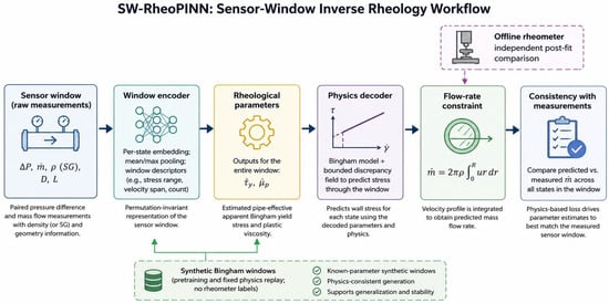
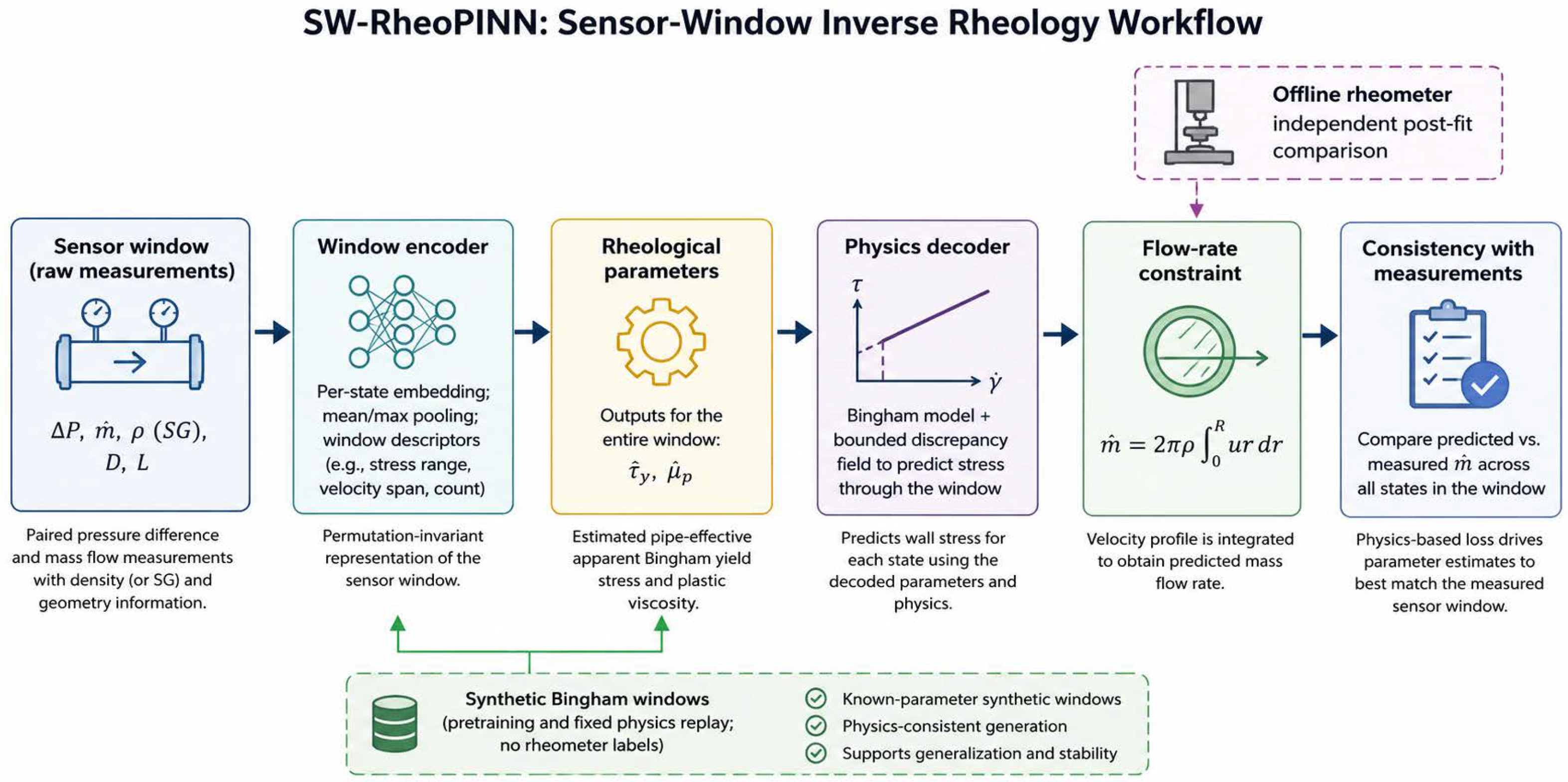
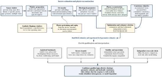
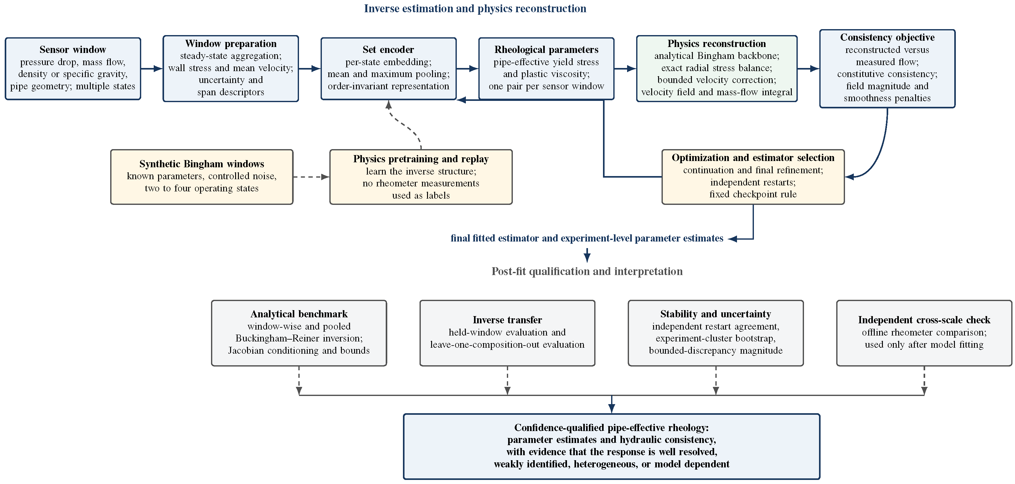
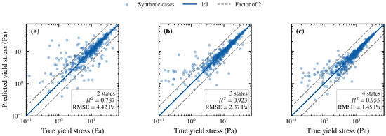
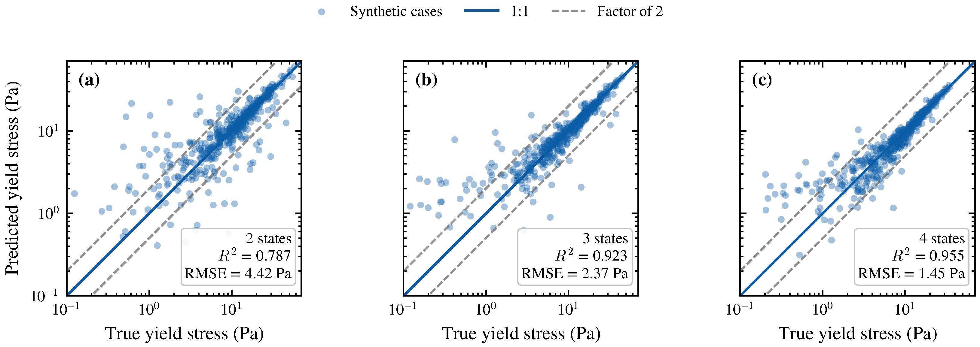
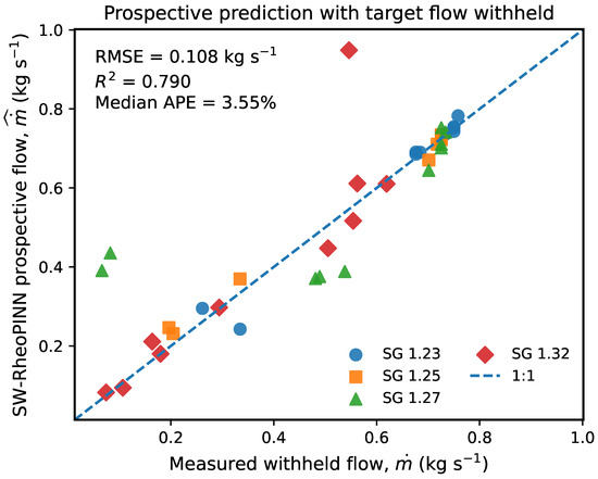
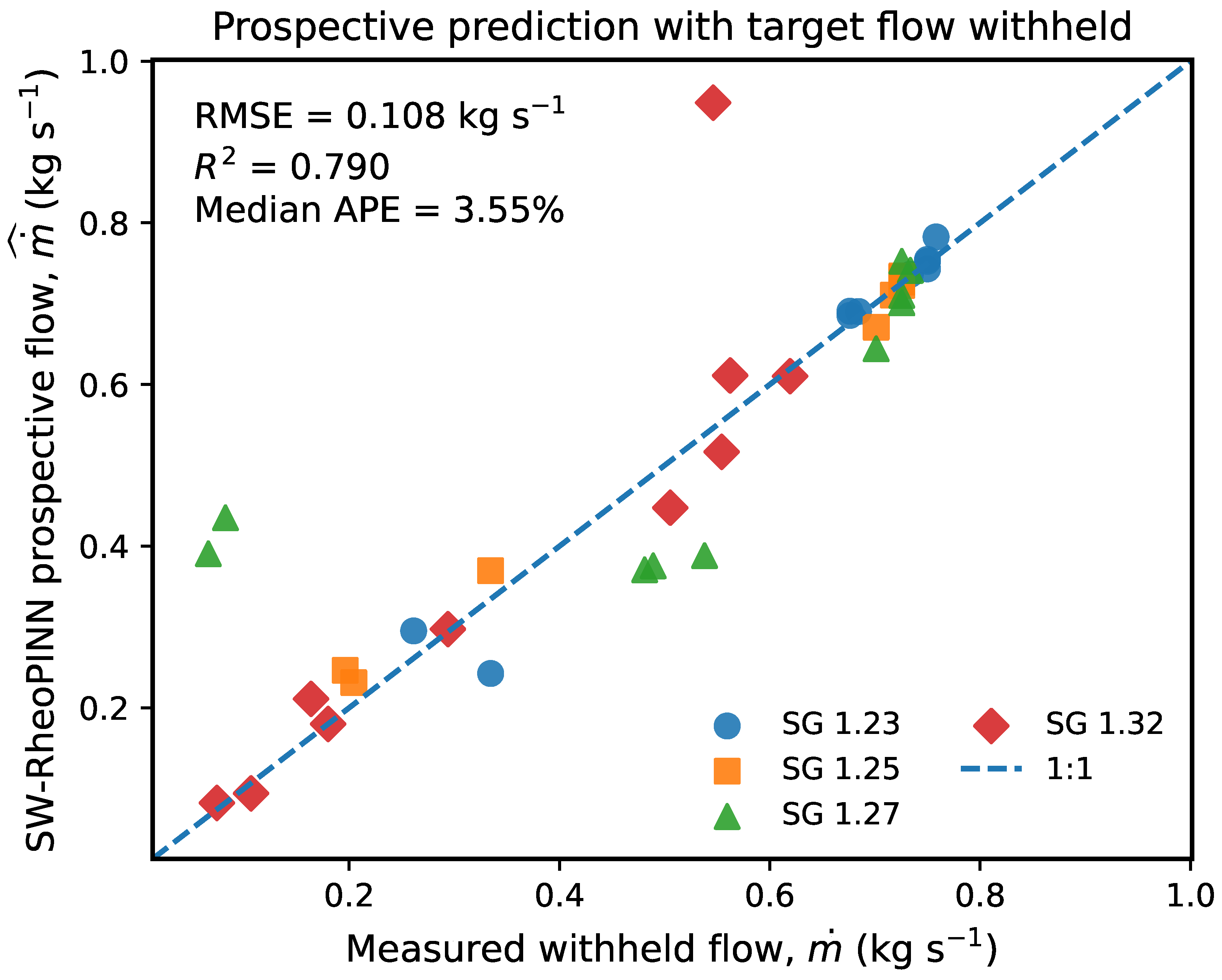
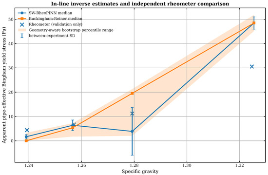
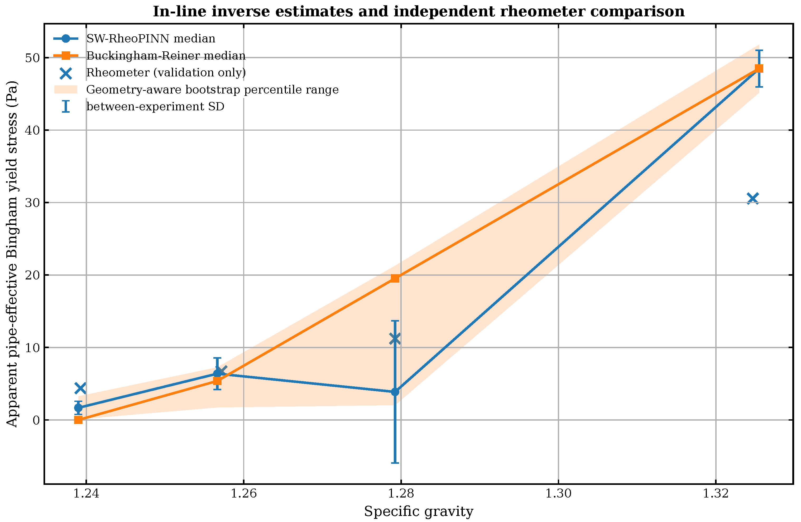
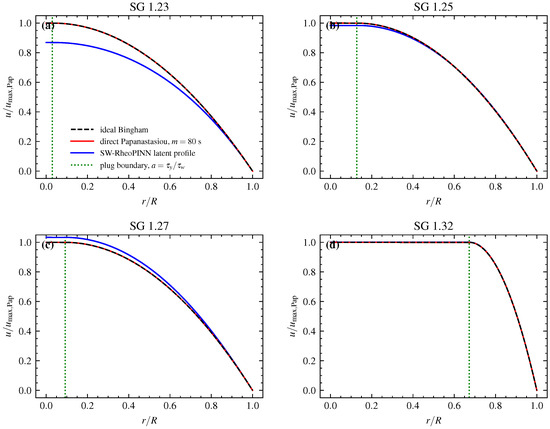
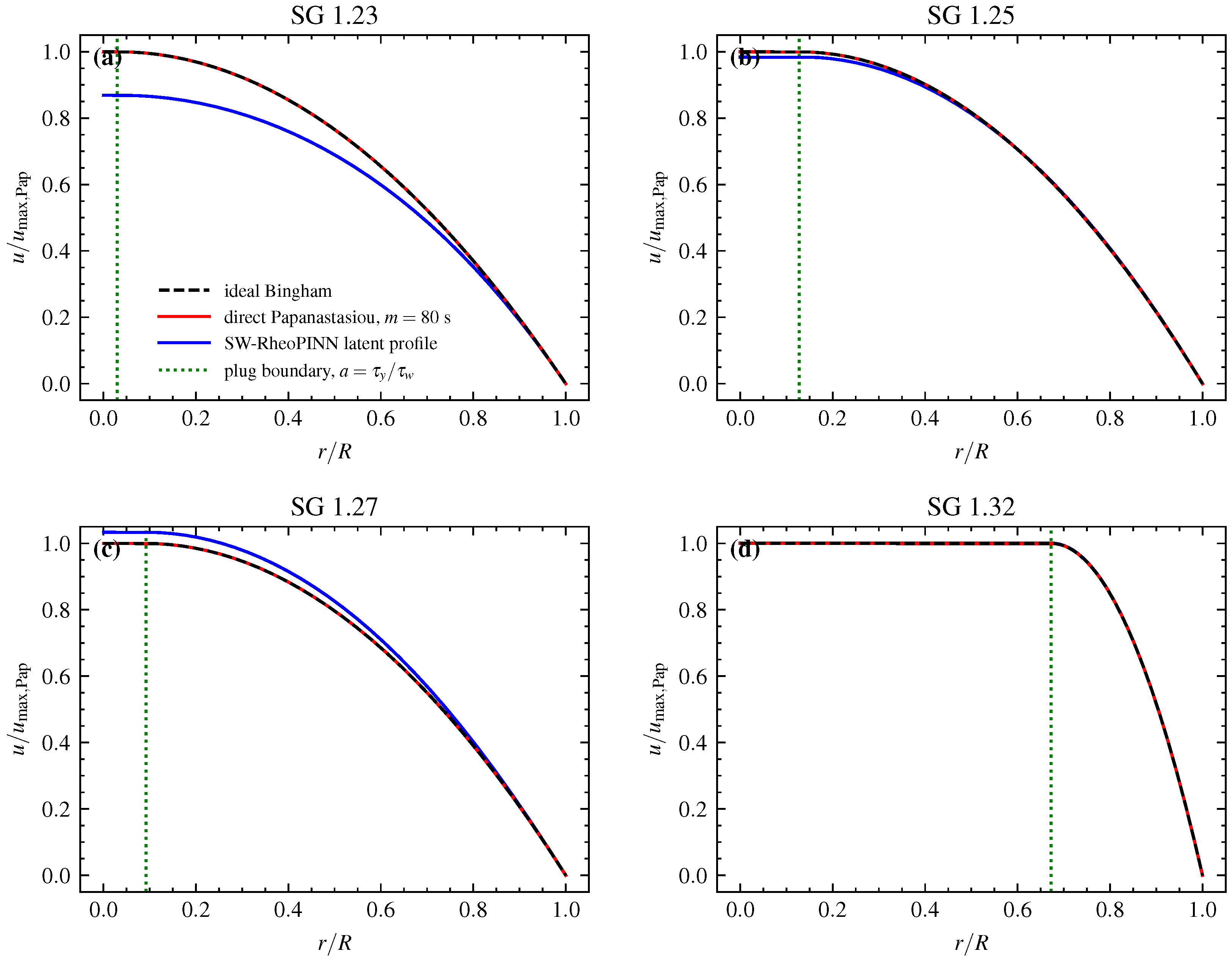
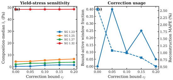
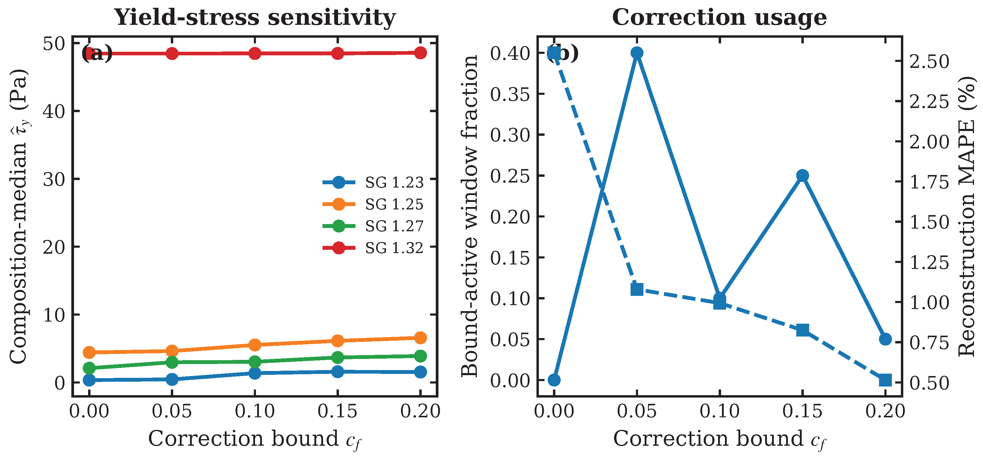

Disclaimer/Publisher’s Note: The statements, opinions and data contained in all publications are solely those of the individual author(s) and contributor(s) and not of MDPI and/or the editor(s). MDPI and/or the editor(s) disclaim responsibility for any injury to people or property resulting from any ideas, methods, instructions or products referred to in the content. |
© 2026 by the authors. Licensee MDPI, Basel, Switzerland. This article is an open access article distributed under the terms and conditions of the Creative Commons Attribution (CC BY) license.