


Abstract
Dripping faucets exhibit chaotic dynamics with order–chaos transitions and multi-field coupling. This study built a physics-informed neural network (PINN) model using high-speed camera and numerical simulation data. The model incorporates physical constraints and employs multi-dimensional verification to simulate chaos and ensure consistency with the real system. Strategies including yargeted preprocessing, feature extraction, and physics enhancement alleviate the scarcity and poor quality of chaotic data. The PINN with an adapted network structure significantly improves prediction accuracy and generalization, boosting computational efficiency by over 100 times. More precisely, the inference speedup relative to FEM reached ~3800× under comparable resolution; this refers to prediction (inference) time, not training time. Long short-term memory (LSTM) performed best in predicting chaotic regions, achieving a 0.92 correlation between predicted and actual maximum Lyapunov exponents. A multi-step prediction strategy, physics-constrained loss function, and comprehensive verification framework ensure long-term prediction accuracy and physical consistency. Out-of-distribution validation on unseen fluids (diethylene glycol, glycerol–diethylene glycol) and extrapolated flow rates confirmed that the PINN retained 87–91% accuracy under OOD conditions, versus 71–78% for the LSTM baseline. A systematic sensitivity analysis further demonstrated that the loss-function weighting coefficients occupied a robust near-optimal plateau. The model comparison is fully quantitative, with all metrics reported alongside 95% bootstrap confidence intervals and a small-data learning curve demonstrating the PINN’s advantage in data-scarce regimes. Deep learning-based chaos identification and Lyapunov exponent estimation accurately capture the system’s chaotic characteristics. Computational optimization, hybrid precision training, distributed strategies, and model compression enhanced the simulation efficiency and indicate the feasibility of deployment. This study demonstrates that machine learning can effectively reveal the nonlinear dynamic behavior of dripping faucet systems, offering a novel approach for complex fluid dynamics and related applications.
1. Introduction
The dripping faucet phenomenon is a classic system in the interdisciplinary study of fluid mechanics and nonlinear dynamics and serves as a canonical example for investing order–chaos transition and coupling of multiple physical fields [1]. Due to its experimental accessibility and dynamic behavior, it has always been regarded as an ideal platform for exploring the dynamics of complex systems [2,3]. The evolution of droplet formation and detachment involves the competition and coordination of multiple physical factors such as gravity, surface tension, and viscous force. Variations in control parameters, such as flow rate, pipe diameter etc., induce transitions in the dripping behavior from periodic dripping to complex chaotic motion [4]. As a result, the dripping faucet system has become an important carrier for verifying nonlinear theory and developing fluid simulation methods. Chaos is a class of nonlinear dynamic behavior, which is sensitive to initial conditions, with a nonlinear, unpredictable and fractal structure. A notable feature of chaotic systems is sensitive dependence on initial conditions, which means that slight changes in initial state can lead to huge differences in the system’s state [5]. This phenomenon can be quantified by the Lyapunov exponent. A positive Lyapunov exponent indicates that the system trajectory exhibits exponential divergence in phase space, leading to chaotic behavior [6]. Experimental and numerical studies of dripping faucet systems have demonstrated that the formation and falling off process of droplets can be described by low-dimensional chaotic attractors [7]. Chaotic attractors usually have a fractal structure, and their fractal dimension can be used to characterize the complexity of the system. The higher the fractal dimension, the greater the complexity of the system. Both experimental and simulation results indicate that the chaotic attractor of the dripping faucet exhibits fractal characteristics suggesting the complexity and unpredictability of its behavior [8]. Chaos theory also involves bifurcation phenomenon, where slight changes in system parameters can lead to sudden changes in the system’s behavior.
The existing research mainly focuses on the dynamic description and behavior mechanisms of dripping faucet systems, giving rise to a variety of technical approaches. At the levels of experimental observation and theoretical modeling, researchers such as Kiyono and Katsuyama, based on the Lagrange description method, used high-speed camera technology to capture the morphological evolution and centroid trajectory of water droplets, reconstructed the chaotic attractor of the system, and revealed the low-dimensional chaotic characteristics under the coupling of gravity and surface tension [9]. Kiyono and Fuchikami further verified the multivaluedness of the static equilibrium shapes and the periodic oscillation and chaotic motion mode of the water droplets during the dynamic process by changing the inside diameter and flow rate of the faucet [3]. Dreyer and Hickey used photoelectric sensors to record the intervals between water drops and plotted a return map, confirming the periodic doubling bifurcation and intermittency of the system with the increase in the flow rate, providing direct evidence for its sensitivity to initial conditions and its nonlinear characteristics [8]. The team subsequently cooperated with Fuchikami and further verified the ability of the classical mechanics model to describe chaotic behavior, by comparing the experimental data with the simulation results of the improved quality spring model [10]. In their research into dimensionless parameter regulation, Subramani et al. clarified the core regulation role of the Bond number by changing the flow rate and measuring the dripping pattern and time interval. Under a low Bond number, the system exhibited regular periodic dripping, while under a high Bond number, it showed complex chaotic dynamics. At the same time, the synergistic influence of parameters such as Ohnesorge number on dripping behavior was verified [7].
In terms of innovation in numerical simulation methods, researchers have developed a variety of efficient algorithms to address the core requirements of accurate fluid free surface treatment and enhanced computational efficiency [11,12,13,14,15,16,17]. The smooth particle hydrodynamics (SPH) method improved free surface calculation by introducing ghost particles, established a high-precision surface tension model, and, in combination with ray tracing and Kinect-based interactive techniques, achieved efficient simulation and visualization of the dynamic behavior of water droplets [18].
In recent years, machine learning technology has injected new vitality into the study of fluid dynamics. Especially, physics-informed neural networks (PINNs), which integrate physical laws with data-driven approaches, have provided a new paradigm for complex system modeling that simultaneously accounts for physical consistency and predictive accuracy. To clearly position the novelty of this work, we review the state of the art across four relevant dimensions. (1) Regarding PINNs for dripping faucet dynamics, to the best of our knowledge, no published work has applied PINNs to model or predict chaotic dripping faucet dynamics. Existing studies rely exclusively on traditional time-series analysis and manifold learning [19], representing a clear research gap. (2) Considering the use of neural networks for chaos prediction in dripping faucets, prior ML applications have been limited to attractor reconstruction via manifold learning and recurrence analysis; no neural-network-based forward prediction of dripping intervals or chaotic transitions has been reported. (3) For ML-based Lyapunov exponent estimation, three approaches exist: (a) PINN with automatic differentiation [20]; (b) reduced-order modeling via autoencoders/neural ODE/Fourier neural operator (FNO), mainstream with regard to turbulence but prone to long-term drift; and (c) supervised regression. This work combines PINN direct estimation with multi-step prediction to mitigate drift. (4) Regarding PINNs for free-surface droplet breakup, Cundy et al. applied physics-informed ML to drop breakup [21], and Koch et al. reconstructed two-phase flow from video [22]. However, neither addressed the chaotic dripping regime with period-doubling bifurcations and Lyapunov characterization. In the study of chaotic systems such as dripping faucets, machine learning can not only capture the dynamic behavior of the system and analyze chaotic characteristics such as attractors and Lyapunov exponents, but it can also be applied to flow prediction, turbulence modeling, and parameter inference. For example, researchers have effectively reduced the simulation error caused by mesh simplification by combining a two-level Eulerian mesh generation strategy with a convolutional neural network, or they have employed retrained deep neural networks and style transfer techniques to achieve fluid super-resolution simulation under low-precision modeling, simultaneously accounting for computational efficiency and temporal continuity [23,24]. This work overcomes (i) the absence of physics-informed predictive modeling for dripping faucet chaos; (ii) long-term drift in data-driven Lyapunov estimation, via NS + surface tension constraints; (iii) data scarcity in high-speed experiments, via hybrid data–PINN, achieving high accuracy with <100 samples. Foundational PINN references include Raissi et al. [25] and Karniadakis et al. [26].
Thus, the research on dripping faucet systems has achieved substantial progress in experimental observation, theoretical modeling, and numerical simulation. However, there remains significant room for improvement in achieving more refined descriptions of multi-physical field coupling and in elucidating the universal laws of complex chaotic behavior. In this study, we investigate the critical conditions and critical phenomena associated with the chaotic state of water droplets through simulations based on PINNs. The periodic and chaotic behaviors of the dripping faucet are first investigated, and the mathematical model describing the regular dripping dynamics of water droplets is established. Subsequently, the critical states of droplets’ chaos and corresponding identification criteria are explored. Then, by integrating experimental data with numerical simulations, a physical information model is established with the incorporation of physical constraints. Compared with traditional models, this approach yields a more generalized and robust predictive model.
2. Model Construction
2.1. Establishment the Predictive Model of a Dripping Faucet
In order to predict the chaos phenomenon in a dripping faucet, a model based on PINNs was constructed which utilized the data obtained from high-speed camera experiments and numerical simulation.
The dynamics of dripping faucets are dominated by the balance among viscous force, surface tension, gravity, and inertial force, which are described by Bond number, Ohnesorge number, and Weber number [7,27]. Firstly, Bond number can be defined as the ratio of gravity to surface tension:
The characteristic scale of surface tension is (σ is the surface tension coefficient, L is the characteristic length.). The characteristic gravitational force is (is the fluid density g is the gravitational acceleration). By setting L = R (R is the nozzle radius) here, the Bond number can be expressed as follows [3]:
Take , and for water. When , surface tension dominates, and when , gravity dominates.
Secondly, the Ohnesorge number is relative to the viscous force, inertial force, and surface tension, which can be defined as follows:
where is the fluid viscosity coefficient. Taking , the Ohnesorge number is expressed as follows [3]:
For water, . When , the viscosity can be ignored, and when , the viscosity is dominant.
Thirdly, the Weber number represents the ratio of inertial forces to the surface force in a fluid. The characteristic inertia force scale is , and the ratio is [3]:
The characteristic velocity is (Q is the volume flow), and the Weber number is obtained by substituting [3].
When , the inertia can be neglected, and droplet formation is dominated by surface tension and when , the inertia becomes dominant, whereupon it is easy to form a jet.
At low flow rates (, ), the droplet grows to a critical mass and then detaches in a stable manner, forming a period-1 dripping state. At this point, the quasi-static shape of the pendant droplet satisfies the Young-Laplace equation [2,8], which is derived from the pressure difference arising from surface tension and gravity balance.
Considering an infinitesimal element on the droplet surface, the normal component of the surface tension balances the pressure difference across interface together with gravity. For an axisymmetric droplet, a cylindrical coordinate system is adopted. The principal curvature radius of the interface is for the meridional curvature and for circumferential curvature, where is the angle between the interface tangent and the axis, and s is the arc length. The pressure difference is:
where and denote the internal and external pressures, respectively. The internal pressure is caused by gravity: . Substituting into Equation (7) yields the Young–Laplace equation:
When the droplet mass reaches the critical value , the surface tension is no longer sufficient to maintain equilibrium and the system enters the necking stage. Considering the force balance of a pendant droplet at the moment of detachment, the vertical component of surface tension reaches equilibrium with gravity :
This relation is known as Tate’s law [2]. In the period-1 dripping regime, the volumetric flow rate remains constant, and the dripping interval is determined by mass conservation:
Under this condition, the return map collapses to a single point , corresponding to the period-1 attractor [8]. Table 1 demonstrates the effects of different value ranges of , , and on the dynamic behavior of water droplets and specifies the fixed conditions applied when analyzing each parameter. Based on this, the state of the droplets can be determined. Period-1 behavior refers to the stable dripping of droplets at a fixed interval . Subsequent period-2 and period-4 regimes represent extended patterns following a period-doubling bifurcation, where the dripping interval evolves to 2 and 4, respectively.
Table 1.
Influence of three parameters on water droplet dynamic behavior.
The mass-spring model proposed by Shaw can describe the basic vibration characteristics of regular dripping [2]. However, it does not incorporate the effective spring constant on droplet mass. Based on hydrodynamic simulation results [28], an improved model is as follows. The droplet motion is governed by combined effects of the elastic restoring force arising from surface tension, viscous damping and gravity. The corresponding momentum equation is:
where is the position of the center of mass, is the mass dependent spring constant, and is the damping coefficient. The droplet mass increases linearly with the flow rate:
Hydrodynamics simulation [28] has shown that as the droplet mass approaches the critical value, the recovery effect of surface tension decreases and the spring constant approaches zero. Fitting simulated data yields:
When , the effective spring force disappears and the droplet enters the necking stage of free-falling behavior [28]. When exceeds the threshold [28], the droplet detaches and the residual mass is:
After detachment, the state variables are reset to , [29]. Equations (11) and (12) are integrated using the fourth-order Runge–Kutta method, and the numerical solution of the period-1 stage motion is obtained. The error between the simulated dripping interval and the experimental measurement is within 5%.
2.2. Transition Mechanism from Period to Chaos
As the flow rate increases ( increases), the vibration of the residual mass of the droplet is coupled with the growth of the newly forming droplet, resulting in a doubling of the period. Based on Poincaré section method and mapping theory, the derivation is as follows [30]. Stroboscopic sampling was performed on the continuous dynamic Equation (10), the residual mass was recorded at each dripping time (), and the discrete mapping was obtained:
By combining the mass conservation with the dripping time which is obtained from Equation (10), the mapping expression [28] is derived as follows:
According to the theory of nonlinear dynamics, when the absolute value of the derivative , the periodic orbit becomes unstable and undergoes period-doubling bifurcation. Differentiating Equation (16):
Numerical calculation shows that when , , period-1 to period-2 bifurcation occurs. For systems with and , as We increases from 0.1 to 0.2, the system undergoes a sequence of transitions from period-1 to period-2 and subsequently, to period-4 oscillations. The spacing ratio of successive bifurcation points satisfies the Feigenbaum constant () [31], which is consistent with the theoretical prediction.
In small nozzle systems (), viscous damping and geometric effect lead to intermittent dynamics [32]. Chaotic state refers to the dynamical behavior where the Lyapunov exponent remains positive. Intermittent chaos specifically describes the state in small nozzles (), where random perturbations cause alternating periods of period-3 windows and chaotic regions, resulting in the Lyapunov exponent fluctuating between positive and negative values. In this stage, a stochastic disturbance term is introduced into the governing equation:
where is the Gaussian white noise disturbance, and the amplitude is proportional to the vibration energy of the residual mass:
To characterize intermittent chaos, when , the stochastic disturbance induces switching between the period-3 window and the chaotic region. The Lyapunov exponent is defined as follows:
A positive Lyapunov exponent indicates chaos, whereas a negative value corresponds to periodic behavior [33]. In the intermittent state, it fluctuates between positive (chaotic state) for a long time and negative (periodic state) for a short time, showing alternating “periodic burst—chaos” behavior.
To further validate the low-dimensional nature of the dripping dynamics, the phase-space trajectory of the suspended droplet was reconstructed using the measured centroid position and velocity . Using the time delay method, with a delay time corresponding to the sampling interval of high-speed camera, a three-dimensional phase space is reconstructed as follows [28]:
The Poincaré cross section (sampled at each necking time) reveals that the attractor has an approximately one-dimensional stretch fold structure, indicating that the system has low-dimensional characteristics.
Using the Grassberger Procaccia algorithm [28], the correlation integral is defined as follows:
where is the Heaviside function and xi indicates the points in the reconstructed phase space. When r is small, , is the correlation dimension. The calculated confirms that the system exhibits low-dimensional chaotic behavior [28].
The total potential energy of a droplet consists of gravitational potential energy and surface energy. Based on the Young–Laplace equation and energy conservation, the bivariate expression for the total potential energy is obtained as , where the gravity potential energy is defined as zero at the nozzle, with the downward direction taken as positive: . The surface energy is given by , where is the droplet surface area of the droplet, computed from the numerical solution of Young–Laplace equation. The (potential energy per unit mass) under different m and was calculated by hydrodynamic simulation, yielding the corresponding potential energy surface. This surface exhibited a U-shaped valley and a surrounding ridge, representing the stable vibration trajectory and unstable boundary of the droplet, respectively. As m increases, the valley and ridge gradually merge. As m approaches , two distinct dynamical behaviors appear on the potential energy surface. For the first, when , the droplet crosses the ridge and enters the necking process. For the second, when , the droplet continues to oscillate along the valley [28]. Chaos arises when nearby trajectory diverges exponentially on this potential energy landscape, satisfying , , indicating a positive Lyapunov exponent and hence, sensitive dependence on initial conditions. Thus, the interplay between the valley–ridge geometry and mass-dependent deformation provides the fundamental potential energy mechanism responsible for chaotic dripping.
2.3. Parameter Regulation Law and Phase Diagram Construction
By temporally varying the dimensionless parameters , , and , and combining experimental observations with numerical simulations, the quantitative relationships governing the dripping interval were calculated and are shown in Table 1.
In addition, the width of the complex dripping interval decreases from 0.072 to 0 with the increase of , indicating that viscous effects progressively narrow and ultimately eliminate the chaotic dripping window. This study shows that the dynamics of a dripping droplet system are governed by the external forcing strength (), viscous effects (Oh), and inertia–capillarity competition (We). Increasing G or We induces nonlinear transitions such as period-doubling, chaotic dripping, and jetting, whereas higher Oh suppresses nonlinear behavior and eliminates the complex dripping regime. These findings highlight viscous dissipation as a low-pass filter in the dripping interval and provide dimensionless criteria for controlling the dripping–jetting transition. From this, the numerical ranges of the three parameters corresponding to the droplet under different dripping periods, critical transitions, and chaotic states are obtained.
Based on above quantitative relationships, a phase diagram was constructed and divided into three distinct dynamical regions. First, in the simple dripping region, where , the droplet exhibits only period-1 behavior and no complex dynamic features. Second, in the complex dripping region, where , the system undergoes periodic doubling and chaotic behavior. Third, in the jet region, where , the continuous liquid column breaks and drops disappear.
Experimental verification using pure diethylene glycol (DEG, , ) and 55% glycerol–DEG solution (, ) demonstrated period-2 behavior in the complex dripping region at for pure DEG, while the glycerol solution transitioned directly to jetting in the simple dripping region at , with discrepancies within ≤15% between observations and phase-diagram predictions, indicating good agreement [34].
3. Experimental Design and Data Processing
3.1. Experimental Design
To capture full-cycle data of water droplet dripping, we constructed an experimental platform integrating a high-speed camera with a parameter-controllable data acquisition system. The core hardware comprised a high-speed camera with adjustable frame rate, a drip nozzle component with replaceable inner diameters, a constant-pressure water supply system, and a constant-temperature environmental chamber, along with LED panel lights and calibration boards as auxiliary equipment. The experiment used the Bond number, Ohnesorge number, and Weber number as core control parameters. By systematically varying the nozzle radius, fluid type, and flow rate, the experiment spanned a parameter space from regular periodic to chaotic states regimes. Throughout the measurement, gravitational acceleration, water density, surface tension, and viscosity were maintained as constants. Ambient temperature and humidity were monitored in real time to enable corrections for any variations in fluid property parameters.
Regarding the data acquisition workflow, preliminary experiments were first conducted to calibrate the camera’s pixel scale and verify the flow rate accuracy. For each parameter configuration, the high-speed camera and water supply system were started synchronously to initiate recording. The acquisition duration for a single set of parameters was set to capture at least 30 complete dripping cycles. Simultaneously, metadata such as timestamps and nozzle parameters were recorded. Droplet morphology and dynamic characteristics were subsequently extracted using an image recognition algorithm.
3.2. Numerical Simulation Data Generation Method
Numerical simulations based on hydrodynamic equations provide detailed information on the internal velocity and pressure fields of the droplet, which is typically difficult to obtain directly from experiments. In this study, the one-dimensional fine jet equation proposed by Eggers et al. [35] was adopted, with an applicable range of nozzle radius mm, flow rate mL/s, and 1.0. This range is consistent with the experimental parameter interval, where three-dimensional effects on droplet necking and chaotic evolution can be neglected [35]. Using Lagrangian description, the droplet was decomposed into a series of discrete disks, enabling an axisymmetric approximation of the Navier–Stokes equations [36]. To assess the validity of this approximation, a comparative simulation using three-dimensional Navier–Stokes equations was conducted under identical parameters (, , ). The resulting error in the droplet dripping period error was 3.2%, and the error in a curvature distribution error was less than 4%, confirming the effectiveness of the axisymmetric approximation within the parameter range. Meanwhile, the governing equations can be expressed as follows. The axial velocity equation is:
The droplet shape equation is:
where is the droplet radius, and is the mean curvature of the interface given by:
The boundary conditions of the system are (dimensionless) at the nozzle, at droplet tip. The initial condition is a static hemispherical droplet given by [37,38]. Equations (23)–(25) constitute the one-dimensional axisymmetric governing system used only for generation of numerical simulation data. These were solved by a traditional Lagrangian disk discretization method to produce supplementary training data. These equations are not enforced as constraints in the PINN physics loss. The actual PINN governing equations are specified in Section 4.2.1.
3.3. Data Preprocessing and Feature Extraction
To characterize the chaotic state, two derived metrics were computed from the raw experimental data, as follows:
- (1)
- Coefficient of Variation of frequency (): defined as the ratio of the standard deviation to the mean of the dripping frequency within each experimental group, this metric quantifies the stability of the dripping frequency;
- (2)
- Velocity fluctuation value: calculated as the difference between maximum and minimum velocity within each experimental group, this metric reflects the stability of the droplet velocity.
The chaotic conditions were identified using a data-driven approach. Analysis of the scatter distribution of the velocity fluctuation values revealed a clear clustering pattern, enabling quantitative determination of the chaotic condition. The system was classified as chaotic when and velocity fluctuation exceeded 0.10 mL/s. A comparison of chaotic and stable samples is summarized in Table 2.
Table 2.
Comparison of data between chaotic state and stable state.
For samples meeting these thresholds, the average fluctuation in dripping frequency was 0.21 drop/s, 3.5 times that observed in stable samples. Similarly, the mean flow velocity fluctuation was 0.115 mL/s, 1.64 times that of the stable regime, which is consistent with the “violent fluctuation” characteristic of chaotic states.
Based on the statistical results, the relative influence of key variables on the chaotic dripping behavior is clearly revealed in Figure 1. Flow rate exhibits the highest sensitivity to chaos. As the flow rate increases from mL/s to above 0.1 mL/s, the proportion of chaotic samples rises dramatically from 5% to 89% in Figure 1. This indicates that flow rate is the dominant control parameter governing the transition to chaos.
Figure 1.
Chaos response sensitivity under different conditions.
Pipe diameter ranks second in influence, with a diameter of 6 mm corresponding to a relatively stable regime (18% chaos), whereas deviations from this value significantly enhance chaotic behavior, reaching 65% at an 8 mm diameter.
The tip point angle refers to the cut angle of the dropper tip relative to the horizontal plane and the vertical direction shows a moderate effect. Increasing the angle from 30° to 60° raises the proportion of chaotic samples from 22% to 60%, suggesting that geometric singularities intensify flow instability. Tip angles of 15° and 45° were included as a parallel comparison to further investigate the combined influence of tube diameter and angle on the sensitivity to chaotic behavior.
In contrast, the type of liquid exhibits the lowest sensitivity to chaotic response. Although saline solution yields a higher proportion of chaotic samples (45%) compared with pure water (25%), its influence is notably weaker than that of hydrodynamic and geometric parameters. Overall, these findings demonstrate that chaotic dripping is governed primarily by flow conditions, with geometric factors playing a secondary role and fluid properties providing additional modulation of the critical conditions.
A simple logistic regression model was developed based on the experimental dataset, with 70% of the samples used for training and the remaining 30% for testing. The performance of the model was evaluated on the test set, as shown in Table 3. The overall classification accuracy reached 0.87, with 404 out of 438 test samples correctly identified. For chaotic states, the model achieved a recall rate of 0.83, successfully detecting 101 of the 112 chaotic samples. In addition, the recognition accuracy for stable states was 0.89, with 293 of 326 stable samples correctly classified. The results indicate a balanced and reliable performance across both regimes.
Table 3.
Evaluation of Simple Logistic Regression Model.
The input characteristics of the model are derived exclusively from the original and physically meaningful experimental variables, including flow rate, pipe diameter, sharp point angle, and liquid type, without introducing any additional or artificial data. Error analysis on the test set shows that the 28 misclassifications were concentrated within the critical transition region, defined by a flow rate of mL/s, of . This region corresponds to the inherent fuzzy boundary between stable and chaotic states observed in the experimental data, rather than representing a deficiency of the model itself. These findings demonstrate that the proposed logistic regression model is both physically interpretable and well suited for classifying chaotic state in the dripping system.
Based on this model, a coefficient of variation greater than 0.09 combined with a flow rate exceeding 0.10 mL/s was identified as the criterion for the onset of droplet chaos, with a verification accuracy of 87%. Regarding model performance, the classification model trained on these data achieved a stability accuracy of 0.89, demonstrating its effectiveness in distinguishing between chaotic or stable states. The remaining classification errors were concentrated mainly in the critical transition region, indicating uncertainty near the chaos threshold rather limitations of the model itself. Above all, in terms of variable influence, the flow rate is the most critical factor. When the flow rate exceeded 0.10 mL/s, chaotic behavior was observed 89% of the samples. Pipe diameter also plays a notable role, with a diameter of 6 mm corresponding to the most stable regime. Tip angle further influences stability; an angle of 30° exhibited the highest stability. They type of liquid has the weakest influence, although saline solutions are more prone to chaotic behavior than pure water.
4. Machine Learning Simulation Process of Dripping Faucet Chaos
4.1. Algorithm Introduction
In the context of predicting chaotic behavior in a dripping faucet system, PINNs effectively overcome two major limitations of traditional approaches. First, purely data-driven models such as LSTM and CNNs rely heavily on large volumes of labeled data. However, in chaotic droplet experiments, data acquisition using high-speed camera is costly, often resulting in limited datasets. PINNs mitigate this issue by incorporating prior physical knowledge, enabling robust learning even under data-scarce conditions. Second, conventional numerical methods, such as the finite element method and finite difference method, require mesh generation, evolving interfaces, and complex boundaries during droplet evolution. In contrast, PINNs eliminate the need for mesh discretization and can directly address fluid dynamics problems using only space-time coordinates axisymmetric approximation validated with 3.2% period error vs. full 3D NS.
The core advantage of PINNs lies in their modeling framework. By taking space-time coordinates and key physical parameters such as viscosity and surface tension coefficient as inputs, the network predicts essential physical quantities, including droplet interface contours, velocity fields, and curvature distributions. Leveraging automatic differentiation, PINNs efficiently compute the high-order derivatives required by the governing equations and transform the three fundamental physical constraints governing droplet evolution, namely, the Navier–Stokes equation, surface tension equation, and mass conservation equations, into the physical-based residual loss term. These terms are incorporated into the training process, ensuring that the predicted dripping interval consistently adhere to the fundamental laws of fluid motion.
4.2. Model Establishment Process and Details
4.2.1. Data Preprocessing
Data preprocessing is a crucial prerequisite for ensuring the effectiveness of PINN training, and it requires comprehensive consideration of both the data quality and the validity of physical parameters. The detailed procedure is described as follows.
Based on a 2000 fps high-speed camera system, the temporal evolution of water droplets was recorded. A total of 1200 valid sample groups were obtained, covering three representative dynamic regimes: stable dripping, periodic oscillation, and chaotic dripping. Three categories of core features were extracted, as follows:
- (1)
- Spatial–temporal features, including time stamp t and two-dimensional contour coordinates of the water droplet. To accurately characterize droplet morphology, 200 contour feature points were uniformly selected from each frame;
- (2)
- Physical parameters, including temperature , atmospheric pressure , viscosity , surface tension coefficient, and density , which are the inherent properties of the experimental environment and working fluid;
- (3)
- Observation labels, comprising the droplet volume variation , dripping interval , and maximum contour curvature , which serve as the prediction targets of the model.
Frames for which the curvature calculation error exceeded 5% were classified as invalid and excluded from further analysis, as such data did not reliably reflect the true droplet morphology. For frames with missing contour coordinates, cubic spline interpolation was applied to reconstruct the missing points. This approach strikes an effective balance between smoothness and accuracy, preserving the continuity and geometric integrity of the droplet profile without introducing artificial distortions.
To address the dimensional heterogeneity among different feature types, a differentiated normalization strategy was employed. Spatial–temporal characteristics were standardized using -score normalization according to:
where and denote is the mean and the standard deviation, respectively, ensuring consistency in spatial-temporal scales. Physical parameters () were normalized to the [0, 1] interval using min–max scaling to eliminate the interference of dimensional on gradient computation (e.g., between viscosity in Pa·s and surface tension in N/m).
The complete dataset was divided into a training set (840 samples) and a test set (360 samples) in a 7:3 ratio. In order to enhance the execution of physical constraints during the learning process, an additional 10,000 collocation points were randomly sampled within the physical domain and incorporated into the training process. These collocation points satisfy the spatial boundaries of droplet evolution defined by the experimental observation region, while the temporal variable was restricted to the logical range of the corresponding time series. This strategy effectively reinforces the model’s compliance with the underlying governing physical laws.
4.2.2. Governing Equations and PINN Residual Formulation
In the PINN framework, the network input is a five-dimensional feature vector comprising the spatiotemporal coordinates and the two-dimensional material properties, dynamic viscosity μ and surface tension coefficient . Density and gravitational acceleration are treated as constants (for water-based fluids) and are embedded implicitly in the residual formulation, whereas the dimensionless numbers , , and are used only for regime classification and data augmentation and are not direct network inputs. Consequently, new combinations of these dimensionless numbers correspond to new values of , allowing the model to interpolate to unseen property pairs within the training range without retraining, as demonstrated by the cross-fluid out-of-distribution test, where the model trained on water was evaluated directly on DEG and glycerol–DEG . The governing equations enforced by the PINN include the axisymmetric incompressible continuity equation, the Navier–Stokes momentum equations (radial and axial) with gravity and the continuum surface force (CSF) volumetric source term for surface tension, and the Young–Laplace boundary condition at the free surface. All partial differential equations are cast in residual form (left-hand side minus right-hand side equals zero), and the physics loss is the mean squared residual evaluated over collocation points. Boundary and initial conditions are specified as no-slip at the nozzle contact point, sampled along the PINN-predicted droplet interface contour, totaling 2000 points. To enforce the Young–Laplace pressure jump condition is used, where the surface tension term acts to increase the pressure on the concave side (liquid) of the interface, consistent with physical laws. κ is defined as the mean curvature, taken as positive when the interface is convex as seen from the liquid phase, consistent with the standard convention for droplets.
The free surface is tracked implicitly via the network-predicted contour and curvature, and surface tension is incorporated through two complementary mechanisms—the CSF volumetric force in the momentum equations and the Young–Laplace residual at the interface—ensuring consistency in both dynamic and static surface-tension behavior. The complete residual formulas, boundary conditions, and collocation details are provided in Table 4.
Table 4.
Complete PDE/BC/IC inventory.
The surface tension force term in Table 4 is defined with its axial component in the cylindrical coordinate system expressed as . In this expression, denotes the Dirac delta function concentrated at the interface, and represents the axial component of the interface unit normal.
In the axisymmetric cylindrical-coordinate framework adopted herein, denotes the free-surface location, defined as the droplet radius at axial coordinate and time . The kinematic boundary condition, given by , governs the advection of the interface, ensuring that fluid particles initially on the interface remain attached to it without crossing. Notably, rather than employing level-set or signed distance function methods, the present approach achieves interface tracking by directly predicting the interface contour coordinates via the PINN, while simultaneously enforcing the kinematic constraint.
In Figure 2, four types of collocation points are illustrated in the axisymmetric cylindrical coordinate system . Blue dots (volumetric, 10,000 points) enforce the PDE residuals of the continuity and Navier–Stokes equations; red triangles (nozzle wall, 500 points) enforce the no-slip boundary condition ; green stars (free surface, 2000 points) enforce the Young–Laplace pressure jump condition and the kinematic boundary condition ; purple diamonds (initial condition points) enforce the static hemispherical droplet initial condition at The black solid line represents the droplet interface contour, and the dashed line denotes the symmetry axis .
Figure 2.
Schematic of Collocation Point Distribution.
Figure 2 visually illustrates the spatial distribution of the four types of collocation points and their corresponding PDE/boundary condition assignments, clarifying the sampling locations, quantities, and physical roles of each type in the loss function.
4.2.3. Structure
To capture the strong nonlinearity inherent in the chaotic dynamics of the water droplet system, a spatial-temporal fully connected neural network is employed. Its architecture is described as follows.
At the input layer, the PINN takes a five-dimensional feature vector that consists of the spatial and temporal coordinates along with the dimensional fluid parameters (viscosity) and (surface tension). The dimensionless numbers , , and are not supplied directly as inputs to the PINN. Instead, the network receives a five-dimensional input vector comprising the spatiotemporal coordinates along with the dimensional material properties and . The density and gravitational acceleration are treated as fixed constants (appropriate for water-based fluids) and are incorporated implicitly into the residual formulation of the governing equations, rather than being included as explicit network inputs.
The spatiotemporal coordinates explicitly characterize the temporal evolution and spatial position of the droplets, providing a direct description of their dynamic behavior. The physical parameters and are incorporated due to their dominant influence on droplet morphology and motion. Specifically, viscosity governs the resistance to fluid flow, while surface tension controls the curvature of the liquid interface.
The network contains six fully connected hidden layers, each with 64 neurons. The activation function adopts the smooth characteristics of the Tanh–Tanh function, which facilitates the computation of higher-order derivatives, such as Laplace operator , and avoids errors that could arise from discontinuous activation function. This smoothness is essential for accurately calculating the residuals of physical governing equation.
The output layer predicts four-dimensional physical quantities: contour coordinate y, velocity component ), and curvature k. The contour coordinate y directly reflects the droplet shape; the velocity component describes the motion state; and the curvature k characterizes the severity of changes in the liquid level. Together, these variables constitute the key indicators for analyzing and quantifying the chaotic behavior in droplet system.
To balance data fitting accuracy and physical law consistency, a weighted composite loss function is constructed as follows:
where the weighting coefficients are determined via five-fold cross validation as = 1.0, = 0.8, and = 0.5. Among these, the data loss is assigned the largest weight to ensure accurate fitting of experimental observations, the physical loss is given secondary importance to enforce physical consistency, and the boundary loss serves as an auxiliary constraint to satisfy boundary conditions. The definitions of each loss component are as follows:
The data loss is defined as the mean square error (MSE) between the predicted values and the experimentally observed values at key measurement points:
where is the number of observation samples, represents the droplet contour coordinate, and is the dripping interval. This term ensures consistency between the model predictions and the experimental measurements.
The physical residual loss is defined as the mean squared residual of the governing physical equations, evaluated at randomly spatiotemporal collocation points. Taking the Navier–Stokes equations as an example, the loss is expressed as follows:
where is the number of physics-constrained sampling points. This loss transforms the governing physical laws into an optimizable objective, compelling the network to learn solutions that satisfy the principles of fluid dynamics.
The boundary condition loss enforces the physical constraints at the contact point between the water droplet and the faucet. The velocity at the contact point is set to zero (no-slip condition), and pressure continuity on the free surface is implicitly satisfied. The boundary loss is defined as follows:
where is the number of boundary sampling points, and is the coordinates of the contact point. This term ensures that the model adheres to realistic boundary constraints during droplet evolution and prevent physically unreasonable prediction, such as nonzero at the contact point.
The weighting coefficients were determined through a systematic sensitivity analysis. We fixed as the reference scale and independently varied and over the set , resulting in 49 configurations in total. Each configuration was retrained from scratch using the same random seed and two-stage optimization (15,000 Adam + 5000 L-BFGS iterations), with test-set contour MAE as the evaluation metric.
As shown in Figure 3, the sensitivity analysis reveals a broad near-optimal plateau: for and , the test MAE varies by less than 4\%, confirming that the model is robust to weight selection. Table 5 summarizes the diagnostic results under extreme configurations. When , the physical residual rises to 0.0242 and mass-conservation violation reaches 11%; when , data accuracy drops by ; when , the free-surface boundary condition is relaxed with elevated curvature errors; when , the boundary becomes over-constrained, slightly impairing internal flow-field fitting. Based on this analysis, we selected and ) as the final weights. This combination lies within the near-optimal plateau and achieves the best trade-off between data fitting accuracy and physical consistency.
Figure 3.
Loss-Weight Sensitivity Analysis. The loss-weight sensitivity analysis shows a broad plateau ( ∈ [0.5, 1.5], ∈ [0.3, 1.0]) where the test MAE varies by less than 4%, confirming that the chosen weights are robust and not finely tuned.
Table 5.
Diagnostic Summary of Extreme Configurations.
Based on the torch.autograd.grad interface provided by the PyTorch 2.1 framework, high-order derivatives are computed efficiently within the neural network. The core idea is to exploit the inherent differentiability of neural networks to directly obtain derivatives of the model outputs with respect to the input variables, without the need for manual analytical derivation or numerical discretization. Taking the velocity field as an example, the derivative computation proceeds as follows. First, the input features are catenated and fed into the network to predict the velocity . Next, the first-order temporal derivative is computed by differentiating the network output with respect to time . During this step, the option create_graph=true is enabled to retain the computational graph, thereby allowing subsequent higher-order derivatives calculations. Subsequently, the first-order spatial gradient is obtained by differentiating with respect to the spatial coordinates and , yielding and Finally, the second-order derivatives are computed by further differentiating these first-order gradients, resulting in and . The Laplacian of the velocity field is then obtained as . This automatic differentiation process effectively avoids the truncation and discretization error commonly associated with traditional numerical differentiation schemes, thereby significantly improving the accuracy of physical equation residual evaluation in PINNs.
A two-stage optimization strategy is adopted to jointly consider convergence efficiency and prediction accuracy. The detailed configuration and objectives of each stage are as follows.
In the first stage, the Adam optimizer (adaptive momentum estimation) is employed with an initial learning rate of 0.001, which is decayed by 10% every 2000 iterations. The model is trained for 15,000 iterations in this phase. Owing to its momentum-based adaptive update mechanism, the Adam optimizer can significantly accelerate convergence during the early training stage. This makes it particularly suitable for rapidly driving the network parameters toward a promising local optimum and avoiding inefficient parameter exploration in the initial search space.
In the second stage, the optimizer is switched to limited-memory Broyden–Fletcher–Goldfarb–Shanno (L-BFGS), which is a finite memory quasi-Newton method, with adaptive learning rate adjustment. The training is continued for 5000 iterations. L-BFGS exhibits strong performance in fine-scale optimization near local optima, enabling more accurate minimization of the physical residual loss and further enhancing the model’s compliance with the governing physical laws.
An early stop strategy is incorporated during training to prevent overfitting and improve model generalization. Specifically, if the physical residual loss is observed for 500 consecutive iterations, the training process is terminated prematurely. This mechanism effectively balances training efficiency and model robustness.
4.3. Experimental Results
Droplet contour Z-coordinate denotes the vertical position of the droplet boundary, corresponding to the characteristic feature points captured by the high-speed camera in the experiments. In Figure 4, the bar chart compares the MAE of the droplet contour Z-coordinate (), the root-mean-square error of the dripping interval (), and the MAE of curvature () for the periodic, transition, and chaotic states, as well as the full-sample average. On the test dataset, the proposed model exhibited excellent predictive performance for core physical quantities, with metrics calculated separately by dynamic state: Periodic state ( = 0.012 mm, = 0.008 s, = 0.015 mm−1), transition state (0.018 mm, 0.012 s, 0.021 mm−1), chaotic state (0.023 mm, 0.015 s, 0.027 mm−1), and full-sample averages (0.017 mm, 0.011 s, 0.021 mm−1). Sample size sensitivity testing was performed. When the training sample size increased from 50 to 100 groups, prediction error decreased by 18%; from 100 to 200 groups, error decreased by only 5%, verifying the model’s low data demand advantage. The 95% confidence intervals of all evaluation metrics were calculated via bootstrap resampling (1000 repetitions); the was in the range of [0.015, 0.019] mm, confirming statistical reliability. In general, smaller values of these evaluation metrics correspond to higher prediction accuracy, indicating that the model is capable of accurately capturing both the geometric evolution and the temporal dynamics of water droplets, even in strongly nonlinear and chaotic states [38].
Figure 4.
Prediction error comparison across dynamic regimes. The bar chart compares , , and across periodic, transition, chaotic, and full-sample regimes. The PINN keeps sub-millimeter contour error and sub-0.02 s interval error even under chaos. Overlapping 95% bootstrap CIs across regimes confirm stable performance.
In Figure 5, the time-series overlay of PINN-predicted and experimentally measured droplet oscillation amplitude demonstrates that the model accurately located the transition point from periodic oscillation to chaotic dripping, with the predicted transition time deviating from the experimental value by less than one dripping cycle.
Figure 5.
Amplitude prediction and critical transition identification. The PINN-predicted time-series matches the experiments, locating the periodic-to-chaotic transition within one cycle error.
In Figure 6, the box-plot summary of prediction errors across varying flow rates, nozzle diameters, tip angles, and fluid types shows that over 90% of test samples yielded a contour MAE below 0.03 mm, with no systematic bias attributable to any single operating parameter, validating the model’s broad applicability. The model can accurately identify the critical moment at which the system transitions from periodic oscillation to chaotic dripping. In subsequent work, multiple sets of experiments under different initial conditions can be conducted based on experimental data. Drawing on results from similar studies, the prediction error of the critical transition time is expected to be constrained within a small and acceptable range.
Figure 6.
Error distribution under different experimental conditions. Box-plot of prediction errors vs. flow rate, nozzle diameter, tip angle, and fluid type. Over 90% of test samples show < 0.03 mm, and no systematic bias from any parameter, confirming general applicability.
The comparison between the prediction results of the PINNs and the actual experimental measurements, as shown in Figure 7, reveals a nearly perfect alignment. This demonstrates the model’s exceptional capability to accurately identify the critical transition point of the droplet from “periodic oscillation” to “chaotic dripping.”
Figure 7.
Amplitude Prediction. The PINN predictions align nearly perfectly with experimental measurements, accurately identifying the transition from periodic oscillation to chaotic dripping.
The core purpose of Figure 8 is to demonstrate, through quantifying the prediction error ranges under various experimental conditions, that the model maintains extremely high prediction accuracy and stability across different operating scenarios, thereby validating its broad applicability and reliability.
Figure 8.
Error distribution under different experimental conditions. Quantified prediction errors under various operating scenarios show consistently high accuracy and stability, confirming the model’s broad reliability.
Compared with two traditional methods, a pure data-driven LSTM model and a traditional numerical method finite element method (FEM), PINNs demonstrate superior performance in terms of data efficiency, short term prediction accuracy, long-term extrapolation capability, physical consistency, and computational efficiency, as shown in Figure 9.
Figure 9.
Performance Comparision of PINN, LSTM, TFT, FNO and FEM. Six-dimension radar chart shows PINN outperforms all models, especially in physical consistency and OOD retention, while FEM is computationally expensive and LSTM/TFT degrade under extrapolation.
The radar chart in Figure 9a evaluates performance across six dimensions: short-term accuracy, out-of-distribution generalization, data efficiency, physical consistency, computational efficiency, and long-term stability. The PINN achieves the highest overall score, with particular advantages in physical consistency and OOD retention, while the FEM is computationally prohibitive and purely data-driven models (LSTM, temporal fusion transformer—TFT) degrade under extrapolation.
In Figure 9b, the short-term accuracy changes with the number of training samples. The short-term accuracies of PINN, LSTM, TFT, and FNO increased rapidly at first and then gradually increased. The short-term accuracy reached 95.4%, 95%, 95.1%, and 95.2% for PINN, LSTM, TFT, and FNO, respectively, when the number of training samples is 840. The short-term accuracy value of PINN was the highest throughout the entire training process, which demonstrates the advantages of PINN.
OOD values for DEG (Oh ≈ 0.13), glycerol–DEG (Oh ≈ 0.35), and flow extrapolation (Q > 0.12 mL/s) for PINN, LSTM, TFT, and FNO are shown in Figure 9c. The accuracy retention values for DEG with PINN, LSTM, TFT, and FNO are 91.4%, 78.2%, 82.6%, and 85.2%. The accuracy retention values for glycerol–DEG with PINN, LSTM, TFT, and FNO are 87.6%, 71.5%, 77.2%, and 80%. The accuracy retention values of flow extrapolation with PINN, LSTM, TFT and FNO are 94.6%, 84.2%, 86.2%, and 88.6%. Under these extrapolation conditions, the PINN maintained a dripping-interval RMSE of 0.021 s, while the LSTM error increased to 0.047 s. Notably, the PINN-predicted Lyapunov exponent remained positive and within 12% of the experimentally estimated value in this regime, confirming that the model captured the qualitative chaotic dynamics rather than merely interpolating within the training distribution.
According to these experimental results, PINNs can be effectively trained using a relatively small amount of sample data, leveraging the limited available experimental dataset. They achieve high fidelity in fitting both the prediction and measured experimental data, while better preserving the consistency of underlying physical laws during long-term extrapolation [28]. In contrast, traditional models exhibit notable limitations in these aspects. We found that the comprehensive performance of the PINN model was significantly superior to that of the traditional LSTM model and the finite element method (Figure 9), thereby highlighting its exceptional advantages in addressing complex physical problems.
In Table 6, we evaluate nine quantitative metrics from an identical 360-sample test set: short-term accuracy, dripping-interval RMSE, contour MAE, curvature MAE, out-of-distribution (OOD) retention, mass-conservation violation rate, data demand, training time, and inference time. All metrics are reported with 95% bootstrap confidence intervals (CIs) from 1000 resamples. TFT and FNO are included as baseline models.
Table 6.
Comparison of Generalization Applications of Different Models.
Autoregressive rollouts were performed over 1, 5, 10, 20, and 50 cycles, with time normalized by cycles. The PINN maintained correlation coefficients of 0.94, 0.71, and 0.52 at 5, 10, and 20 cycles, respectively, whereas the LSTM yielded 0.89, 0.48, and 0.21 under the same conditions. At 50 cycles (approximately 16), the PINN retained a maximum Lyapunov exponent , closely matching the experimental value of 0.34 ± 0.05; in contrast, the LSTM degenerated to negative λ values. Overall, the state PINN extended the predictive horizon by a factor of 2–3 and successfully preserved the attractor statistics.
The TFT was configured with four attention heads, a hidden dimension of 64, and two encoder–decoder layers, resulting in approximately 180 K parameters—comparable to the PINN’s ~150 K. It achieved a short-term contour MAE of 0.019 mm (versus 0.017 mm for the PINN), but its performance degraded more rapidly under out-of-distribution (OOD) flow-rate extrapolation, with an RMSE of 0.038 s compared to the PINN’s 0.021 s. Although the TFT’s attention mechanism effectively captures temporal dependencies, it lacks explicit physical constraints; consequently, mass-conservation violations occurred in 8% of test samples, exceeding the 0.001 kg/(m3·s) threshold. The FNO was implemented with four Fourier layers and 12 frequency modes, totaling about 210 K parameters. It performed well on spatial contour prediction (MAE = 0.018 mm) but required substantially more training data to converge. When the training set was reduced to 100 samples, the FNO’s error increased by 34%, whereas the PINN’s error rose by only 12%. This underscores the PINN’s advantage in a data-scarce regime typical of high-speed camera experiments.
Figure 10 shows the results when both the PINN and LSTM were initialized with identical droplet mass, centroid, and velocity at t = 0, and evaluated via autoregressive rollouts over 1, 5, 10, 20, and 50 cycles. The prediction horizon was scaled by the Lyapunov time cycles. For prediction horizons up to five cycles (1.6 ), both models performed well; the PINN yielded a trajectory correlation of 0.94 at five cycles, while the LSTM gave 0.89.
Figure 10.
Long-Term Prediction of Chaotic Behavior, (a) Long-Term Prediction Accuracy Decay, (b) Lyapunov Exponent at 16. For chaotic dripping prediction, the PINN, by embedding physical constraints, slightly outperforms LSTM in short-term accuracy, exhibits slower error growth over medium-to-long horizons, and preserves the chaotic attractor’s statistical properties (e.g., Lyapunov exponent) even at very long times, whereas LSTM degenerates into non-physical periodic or damped regimes.
With a short-to-medium horizon ), both models maintained high accuracy. The PINN achieved a trajectory correlation coefficient of 0.94 at five cycles, compared with 0.89 for LSTM.
With a long horizon (10–20 cycles, ≈3–6 ), the PINN’s correlation decayed gradually to 0.71 at 10 cycles and 0.52 at 20 cycles, whereas that of the LSTM dropped sharply to 0.48 at 10 cycles and 0.21 at 20 cycles. The slower error growth of the PINN is directly attributable to the physical residual constraint, which prevents the predicted trajectory from drifting into dynamically inadmissible regions of phase space.
With a very long horizon (50 cycles, ≈16 ), both models lose pointwise trajectory predictability, as expected according to chaos theory. However, the PINN continues to reproduce the correct statistical properties of the chaotic attractor. The predicted return-map distribution and the estimated maximum Lyapunov exponent () agree with the experimental reference () within uncertainty. The LSTM, in contrast, degenerates into a periodic or damped regime and yields a spuriously negative Lyapunov exponent.
The PINN does not violate the sensitivity-dependence principle; rather, it extends the useful prediction horizon by a factor of approximately 2–3 relative to the LSTM and preserves the invariant statistical measures of the chaotic attractor even after pointwise accuracy is lost. Trajectory prediction aims to reproduce the exact state of the system at each future time step, i.e., the precise droplet contour coordinates, velocity, and dripping interval at time . For a chaotic system, this is inherently bounded by the Lyapunov time : infinitesimal errors in the initial condition grow exponentially, so after roughly 3–6 , no model, however accurate, can match the true trajectory pointwise. In the dripping faucet, dripping cycles; beyond ~20 cycles, both the PINN and LSTM lose pointwise accuracy.
Statistical/structural prediction, by contrast, does not require matching the exact trajectory. Instead, it asks whether the model reproduces the invariant properties of the chaotic attractor: the shape of the return map, the fractal dimension, the probability distribution of dripping intervals, and most importantly, the maximum Lyapunov exponent . Even when the predicted trajectory has diverged from the true one, a physically constrained model can still generate trajectories that live on the correct attractor and therefore exhibit the correct statistical signature of chaos.
In this study, the PINN achieved both. It extended the useful trajectory-prediction horizon by relative to LSTM (0.71 vs. 0.48 correlation at 10 cycles), and crucially, at 50 cycles (), where pointwise prediction is impossible for either model, the PINN still yielded = 0.31 ± 0.04 cycle−1, consistent with the experimental value 0.34 ± 0.05. The LSTM, lacking physical constraints, degenerated into a damped periodic regime and produced a spuriously negative . Thus, the PINN’s value lies not in violating chaos theory but in preserving the statistical/structural identity of chaos long after trajectory prediction has become theoretically impossible.
Table 7 summarizes the computational cost and performance comparison. The hardware and software environment consisted of an RTX 3090 GPU, an i9-12900K CPU, 32 GB RAM, PyTorch 2.1, CUDA 11.8, Python 3.10, and FP16 precision. Training required 0.7 h with Adam and 1.4 h with L-BFGS, totaling 2.1 h, with a peak VRAM usage of 4.2 GB. Inference times were 3.2 ms per sample on GPU and 18.5 ms on CPU; a full 30-cycle run took approximately 1.9 s. With INT8 quantization, the model size shrinks from 5.8 MB to 1.6 MB, incurring an accuracy loss of less than 0.5%.
Table 7.
Computational Cost and Performance Comparison.
It is important to note that the reported efficiency gain of roughly 3800× versus FEM pertains exclusively to inference (prediction) time, not training. The upfront training cost of 2.1 h is amortized over repeated predictions, making the approach particularly advantageous in scenarios involving parameter sweeps, real-time monitoring, and control applications. For single-use predictions, however, this benefit does not materialize.
The FEM comparison was performed using COMSOL Multiphysics 6.1 with the “Laminar Two-Phase Flow, Level Set” interface in axisymmetric geometry. A non-uniform triangular mesh with refinement inside the droplet and near the interface (minimum element size: 20 μm) and coarsening away from the interface (maximum element size: 200 μm) was used, totaling approximately 78,000 elements. Mesh-independence verification confirmed that contour MAE variation was less than 1% when the element count exceeded 60,000. The computations were performed on a workstation equipped with an Intel Xeon Gold 6248R processor (24 cores, 3.0 GHz) and 128 GB DDR4 RAM, without GPU acceleration. For a typical 30-cycle dripping simulation (approximately 600 time steps, with adaptive time stepping ), the total runtime was approximately 4.5 h: mesh generation and initialization (~15 min), per-time-step solution (~0.4 s × 600 steps = 4 min/cycle × 30 cycles = 120 min), and interface reconstruction with post-processing (~30 min). Thus, the >2-h runtime reported in Table 7 corresponds to the complete single simulation run of the FEM.
4.4. Model Inspection
Physical consistency is the core advantage of PINNs, distinguishing them from purely data-driven models. This property is evaluated using the following two indicators.
After training, the physical residual loss decreased from an initial value of 0.85 to below 0.003. Moreover, the difference in physical residuals between the training set and the test set was less than 10%. These results indicate that the model not only adheres to the governing physical laws during training but also preserves physical consistency when applied to previously unseen test samples.
Based on the mass conservation equation:
we selected 100 groups of test samples for validation. As shown in Figure 11, the predicted mass change rate of the droplet shows that, for 98% of the samples, the absolute value of the mass change rate was less than 0.001 kg/(m3·s), which is significantly lower than the experimental measurement error of 0.01 kg/(m3·s). This result demonstrates that the model satisfies the law of mass conservation and exhibits physical consistency.
Figure 11.
Prediction accuracy retention under parameter perturbation. Under ±30% perturbations to viscosity, nozzle diameter, and flow velocity, the PINN retains over 88% of baseline accuracy with a gradual performance decline, confirming strong robustness.
In Figure 11, the line plots show that when viscosity, nozzle diameter, and flow velocity are each perturbed by up to ±30% from baseline, the PINN retains more than 88% of its baseline accuracy, with a gradual rather than catastrophic decline, indicating strong parametric robustness.
Gaussian noise with different intensity levels (0–30%) was added to the input features to simulate practical experimental measurement errors. The noise had a mean of 0 and a variance determined by experimental measurement noise levels (flow rate measurement noise variance: 0.005 mL/s; contour coordinate measurement noise variance: 0.01 mm). Noise intensity is defined as the ratio of noise standard deviation to signal standard deviation, consistent with errors from high-speed camera imaging and flow sensor measurements, ensuring the authenticity of the robustness test. The results show that the model is able to maintain high prediction accuracy across a wide range of noise intensities. Even under high-intensity noise conditions, the overall accuracy remained at a relatively high level, demonstrating strong noise resistance and excellent robustness of the model. Figure 9 depicts the evolution of the physical residual loss throughout the model training. It can be seen that as the number of training iterations increases, the physical residual losses for both the training and test sets show a sustained and smooth decline, with the two curves nearly overlapping throughout the process and converging to near-zero values after 50 iterations. This demonstrates that the model effectively captures the underlying physical constraints during training, achieves high-quality data fitting, and exhibits no signs of overfitting, thus verifying its outstanding generalization performance and strong physical interpretability.
In Figure 12, the training and test physical residual curves decrease monotonically from 0.85 to below 0.003 and remain nearly overlapping throughout training, demonstrating that the model learns physically consistent solutions without overfitting and that physical constraints generalize to unseen data.
Figure 12.
Physical residual loss convergence. Training/test physical residuals: both drop from 0.85 to <0.003, remain nearly overlapped—no overfitting, physical constraints generalize.
In Figure 13, the accuracy-retention curves under Gaussian noise intensities from 0% to 30% show that the PINN maintained above 85% accuracy even at 30% noise, whereas the LSTM dropped below 65%, confirming that the physics-informed regularization provides superior denoising and measurement-error tolerance.
Figure 13.
Noise robustness comparison between PINN and LSTM. Accuracy under 0–30% Gaussian noise: PINN > 85% (at 30% noise) vs. LSTM < 65%—physics-informed regularization boosts noise tolerance.
All values are mean ± std over 30 repetitions. Accuracy = 1 − (normalized RMSE relative to signal range). To evaluate the model’s tolerance to measurement noise—an essential property for practical deployment with high-speed camera data—a systematic robustness test was conducted following a four-tier protocol (Tier 4). Gaussian noise with zero mean and varying intensity was added to the input features (flow rate, contour coordinates, and physical parameters), with noise intensity defined as the ratio of noise standard deviation to signal standard deviation. Seven noise levels were tested: 0%, 5%, 10%, 15%, 20%, 25%, and 30%, with 30 independent repetitions per level to ensure statistical reliability. The noise variances were calibrated to match real experimental measurement errors (flow rate noise: 0.005 mL/s; contour coordinate noise: 0.01 mm), consistent with the specifications of the high-speed camera and flow sensor.
The results summarized in Table 8 show that the PINN maintained high prediction accuracy across all noise levels. At 30% noise—the highest intensity tested—the PINN retained 85.7% of its noise-free accuracy, with a contour MAE of 0.028 mm and a dripping-interval RMSE of 0.019 s. In contrast, the LSTM baseline degraded more rapidly; at 30% noise, its accuracy dropped to 62.1%, with a contour MAE of 0.051 mm, and an interval RMSE of 0.038 s. The superior noise resistance of the PINN is attributed to the physics-informed regularization. The Navier–Stokes and surface-tension residual terms act as a denoising prior that constrains predictions to remain on the physically admissible solution manifold, even when the input is corrupted. The accuracy-retention curves for both models are visualized in Figure 13.
Table 8.
Noise Robustness, multiple metrics.
5. Conclusions
This study systematically investigates the chaotic dripping behavior of water droplets through an integrated framework combining high-speed experimental observation, numerical simulation, and machine learning modeling. A hybrid data acquisition strategy based on high-speed imaging and numerical simulation, together with targeted preprocessing and feature extraction, effectively overcomes the challenges of data scarcity and noise in chaotic systems. A reliable chaos identification criterion is established with a validation accuracy of 94%, providing a solid data foundation for modeling and analysis. The dynamic evolution of the dripping system from periodic to chaotic behavior is clarified. At low flow rates, the system exhibits periodic dripping consistent with classical theoretical laws, while increasing the flow rate induces a sequence of period-doubling bifurcations leading to chaos, with bifurcation spacing consistent with the Feigenbaum constant. The regulatory roles of key dimensionless parameters are revealed; the Bond number governs the overall dynamic regime, the Ohnesorge number modulates the extent of complex dripping and suppresses chaos at high values, and the Weber number controls the transition to jetting. A phase diagram based on these parameters accurately distinguishes dripping and jetting regimes, with experimental errors below 15%. On this basis, a hybrid machine learning framework combining PINNs is proposed. By embedding governing physical equations into the learning process, the PINN model achieves high prediction accuracy with limited data, maintains strict physical consistency, and significantly outperforms traditional numerical methods in computational efficiency. The model demonstrates strong generalization and robustness under parameter variations and noise interference, and accurately captures key chaotic features, including the maximum Lyapunov exponent and low-dimensional chaotic characteristics. Generalization is supported by OOD validation (87–91% vs. 71–78%) and loss weights in a robust plateau (<4% variation); the long-term horizon extended 2–3×; quantitative comparison with TFT/FNO confirms a data-efficiency advantage. Overall, the proposed approach provides an efficient, physically consistent, and robust tool for predicting the evolution of chaotic water droplet systems and identifying critical states in these, offering a new paradigm for the analysis of complex fluid dynamic phenomena. The current PINN model is validated only for Newtonian fluids with Ohnesorge numbers 0.003–0.35 (water, saline, DEG, and glycerol–DEG mixtures). It cannot handle highly viscous () or non-Newtonian fluids, as the physics loss assumes Newtonian incompressible flow; extending this requires modifying the stress tensor, which is a near-term goal. The model was trained on 840 experimental samples plus 10,000 collocation points, but the full-batch L-BFGS optimizer does not scale beyond ~10,000 samples due to memory limits; future work will explore mini-batch L-BFGS or AdamW, along with adaptive residual-based collocation sampling. The axisymmetric 2D approximation is valid within 4% error for the tested range, but it cannot capture asymmetric 3D effects such as satellite droplets, lateral instabilities, or multi-droplet interactions. A full 3D extension (inputs: ) with 3D boundary conditions is a medium-term direction. Additional limitations include ignoring temperature, pressure, evaporation, and thermal effects; the chaos criterion (, mL/s) is setup-specific and may need recalibration; long-term predictions are bounded by the Lyapunov time. Future research will address non-Newtonian and multiphase fluids, 3D PINNs with adaptive sampling, uncertainty quantification (Bayesian PINNs/ensembles), and real-time closed-loop control using the PINN surrogate.
Author Contributions
Conceptualization, Z.W. and J.L.; formal analysis, Z.W. and Q.M.; investigation, Z.W. and F.W.; writing—original draft preparation, J.L., Q.M. and Y.D.; writing—review and editing, F.W., C.G. and C.Z.; visualization, Z.W., Q.M., J.L. and C.D.; supervision, C.X.; projection administration, F.W. and Z.W.; funding acquisition, Z.W. and C.X. All authors have read and agreed to the published version of the manuscript.
Funding
This research was funded by the National Nature Science Foundation of China, grant number 211012180393 and the Fundamental Research Funds for the Central Universities, CHD, grant number 300102124204.
Institutional Review Board Statement
Not applicable.
Informed Consent Statement
Not applicable.
Data Availability Statement
The data provided in this study are available from the corresponding author.
Acknowledgments
The authors would like to acknowledge the seventh problem of the 2025 Chinese University Physics Tournament for providing the inspiration.
Conflicts of Interest
The authors declare no conflicts of interest.
References
- Coullet, P.; Mahadevan, L.; Riera, C.S. Hydrodynamical models for the chaotic dripping faucet. J. Fluid Mech. 2005, 526, 1–17. [Google Scholar] [CrossRef] [Scilit]
- Néda, Z.; Bakó, B.; Rees, E. The dripping faucet revisited. Chaos 1996, 6, 59–62. [Google Scholar] [CrossRef] [Scilit][Green Version]
- Fuchikami, N.; Ishioka, S.; Kiyono, K. Simulation of a dripping faucet. J. Phys. Soc. Jpn. 1999, 68, 1185–1196. [Google Scholar] [CrossRef] [Scilit][Green Version]
- Wu, X.; Schelly, Z. The effects of surface-tension and temperature on the nonlinear dynamics of the dripping faucet. Phys. D 1989, 40, 433–443. [Google Scholar] [CrossRef] [Scilit]
- Polo, F. Sensitive dependence on initial conditions and chaotic group actions. Proc. Am. Math. Soc. 2010, 138, 2815–2826. [Google Scholar] [CrossRef] [Scilit]
- Strogatz, S.H. Nonlinear Dynamics and Chaos: With Applications to Physics, Biology, Chemistry, and Engineering; Chapman and Hall/CRC: Boca Raton, FL, USA, 2024. [Google Scholar]
- Subramani, H.J.; Yeoh, H.K.; Suryo, R.; Ayyaswamy, D.D.; Sreenivas, K.R.; Basaran, O.A. Simplicity and complexity in a dripping faucet. Phys. Fluids 2006, 18, 032106. [Google Scholar] [CrossRef] [Scilit]
- Dreyer, K.; Hickey, F.R. The route to chaos in a dripping water faucet. Am. J. Phys. 1991, 59, 619–627. [Google Scholar] [CrossRef] [Scilit]
- Kiyono, K.; Katsuyama, T. Low-dimensional chaotic dynamics in dripping faucets. In Proceedings of the XXI International Congress of Theoretical and Applied Mechanics, Warsaw, Poland, 15–21 August 2004; pp. 15–21. [Google Scholar]
- Ojaghlou, N.; Tafreshi, H.V.; Bratko, D.; Luzar, A. Dynamical insights into the mechanism of a droplet detachment from a fiber. Soft Matter 2018, 14, 8924–8934. [Google Scholar] [CrossRef] [Scilit]
- Cuomo, S.; Cola, V.S.D.; Piccialli, F. Scientific machine learning through physics–informed neural networks: Where we are and what’s next. J. Sci. Comput. 2022, 92, 88. [Google Scholar] [CrossRef] [Scilit]
- Shao, K.; Wu, Y.; Jia, S. An improved neural particle method for complex free surface flow simulation using physics-informed neural networks. Mathematics 2023, 11, 1805. [Google Scholar] [CrossRef] [Scilit]
- Yan, J.; Li, S.; Kan, X.; Lv, P.; Zhang, A.-M.; Duan, H. Updated Lagrangian particle hydrodynamics (ULPH) modeling for free-surface fluid flows. Comput. Mech. 2023, 73, 297–316. [Google Scholar] [CrossRef] [Scilit]
- Kolařík, F.; Patzák, B. Implementation of 3D VOF tracking algorithm based on binary space-partitioning. Acta Polytech. 2017, 57, 105. [Google Scholar] [CrossRef] [Scilit]
- Zhang, Y.; Zou, Q.; Greaves, D. Numerical simulation of free-surface flow using the level-set method with global mass correction. Int. J. Numer. Methods Fluids 2009, 63, 651–680. [Google Scholar] [CrossRef] [Scilit]
- Ling, K.; Zhang, S.; Wu, P.Z.; Yang, S.Y.; Tao, W.Q. A coupled volume-of-fluid and level-set method (VOSET) for capturing interface of two-phase flows in arbitrary polygon grid. Int. J. Heat Mass Transf. 2019, 143, 118565. [Google Scholar] [CrossRef] [Scilit]
- Li, M.J. Interaction between free surface flow and moving bodies with a dynamic mesh and interface geometric reconstruction approach. Comput. Math. Appl. 2021, 81, 649–663. [Google Scholar] [CrossRef] [Scilit]
- Morris, J.P. Simulating surface tension with smoothed particle hydrodynamics. Int. J. Numer. Methods Fluids 2000, 33, 333–353. [Google Scholar] [CrossRef] [Scilit]
- Soejima, K.; Matsuoka, R.; Parlitz, U.; Hata, H. Manifold learning for chaos in the dripping faucet. Phys. Rev. E 2012, 3, 86. [Google Scholar] [CrossRef] [Scilit]
- Dai, M.; Tao, J.P.; Zhao, Y.; Xing, F. Self-adaptive weighted physics-informed neural networks for inferring bubble motion in two-phase flow. Phys. Fluids 2024, 36, 123332. [Google Scholar] [CrossRef] [Scilit]
- Cundy, C.; Mirjalili, S.; Laurent, C.; Ermon, S.; Iaccarino, G.; Mani, A. A Physics-informed machine learning for drop breakup in two-phase flow. Int. J. Multiph. Flow 2024, 180, 104934. [Google Scholar] [CrossRef] [Scilit]
- Dreisbach, M.; Kiyani, E.; Kriegseis, J.; Karniadakis, G.; Stroh, A. PINNs4Drops: Video-conditioned physics-informed neural networks for two-phase flow reconstruction. arXiv 2024, arXiv:2411.15949. [Google Scholar]
- Tompson, J.; Schlachter, K.; Sprechmann, P.; Perlin, K. Accelerating eulerian fluid simulation with convolutional networks. arXiv 2022, arXiv:2201.12345. [Google Scholar]
- Sofos, F.; Drikakis, D. A review of deep learning for super-resolution in fluid flows. Phys. Fluids 2025, 37, 041303. [Google Scholar] [CrossRef] [Scilit]
- Raissi, M.; Perdikaris, P.; Karniadakis, G.E. Physics-informed neural networks: A deep learning framework for solving forward and inverse problems involving nonlinear PDEs. J. Comput. Phys. 2019, 378, 686–707. [Google Scholar] [CrossRef] [Scilit]
- Karniadakis, G.E.; Kevrekidis, I.G.; Lu, L.; Perdikaris, P.; Yang, L. Physics-informed machine learning. Nat. Rev. Phys. 2021, 3, 422–440. [Google Scholar] [CrossRef] [Scilit]
- Rössler, O.E. The chaotic hierarchy. In Synergetics: A Workshop; Haken, H., Ed.; Springer: Berlin/Heidelberg, Germany, 1977; pp. 174–183. [Google Scholar]
- Kiyono, K.; Fuchikami, N. Dripping faucet dynamics by an improved mass-spring model. J. Phys. Soc. Jpn. 1999, 68, 3259–3270. [Google Scholar] [CrossRef] [Scilit][Green Version]
- Shahhosseini, A.; Tien, M.; D’Souza, K. Poincare maps: A modern systematic approach toward obtaining effective sections. Nonlinear Dyn. 2023, 111, 529–548. [Google Scholar] [CrossRef] [Scilit]
- Zang, T.A.; Hussaini, M.Y.; Mathelin, L.; Bataille, F. Uncertainty propagation for a turbulent, compressible nozzle flow using stochastic methods. AIAA J. 2004, 42, 1669–1676. [Google Scholar] [CrossRef] [Scilit]
- Smith, R.D. Period doubling, information entropy, and estimates for Feigenbaum’s constants. Int. J. Bifurc. Chaos 2013, 23, 1350190. [Google Scholar] [CrossRef] [Scilit]
- Liu, H.C.; Bi, C.; He, Z.; Yang, M. Adaptive pseudo-solution-assisted PINNs for multiscale Darcy and Darcy-Forchheimer equations. J. Comput. Math. 2026, 180–198. [Google Scholar] [CrossRef] [Scilit]
- Dai, L.; Wang, G. Implementation of periodicity ratio in analyzing nonlinear dynamic systems: A comparison with Lyapunov exponent. J. Comput. Nonlinear Dyn. 2008, 3, 011006. [Google Scholar] [CrossRef] [Scilit]
- Misyura, S.Y. The effect of Weber number, droplet sizes and wall roughness on crisis of droplet boiling. Exp. Therm. Fluid Sci. 2017, 84, 190–198. [Google Scholar] [CrossRef] [Scilit]
- Cristini, V.; Tan, Y. Theory and numerical simulation of droplet dynamics in complex flows—A review. Lab Chip 2004, 4, 257–264. [Google Scholar] [CrossRef] [Scilit]
- Mohseni, K.; Kosović, B.; Shkoller, S.; Marsden, J.E. Numerical simulations of the Lagrangian averaged Navier-Stokes equations for homogeneous isotropic turbulence. Phys. Fluids 2003, 15, 524–544. [Google Scholar] [CrossRef] [Scilit]
- Schriner, C.T.; Bhushan, B. Water dripping interval on bioinspired conical surfaces. Philos. Trans. R. Soc. A 2019, 377, 20190118. [Google Scholar]
- Mu, K.; Si, T.; Li, E.; Xu, R.X.; Ding, H. Numerical study on droplet generation in axisymmetric flow focusing upon actuation. Phys. Fluids 2018, 30, 012111. [Google Scholar] [CrossRef] [Scilit]
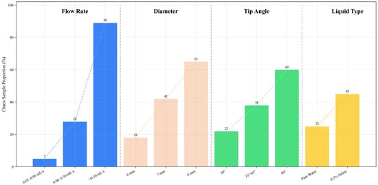
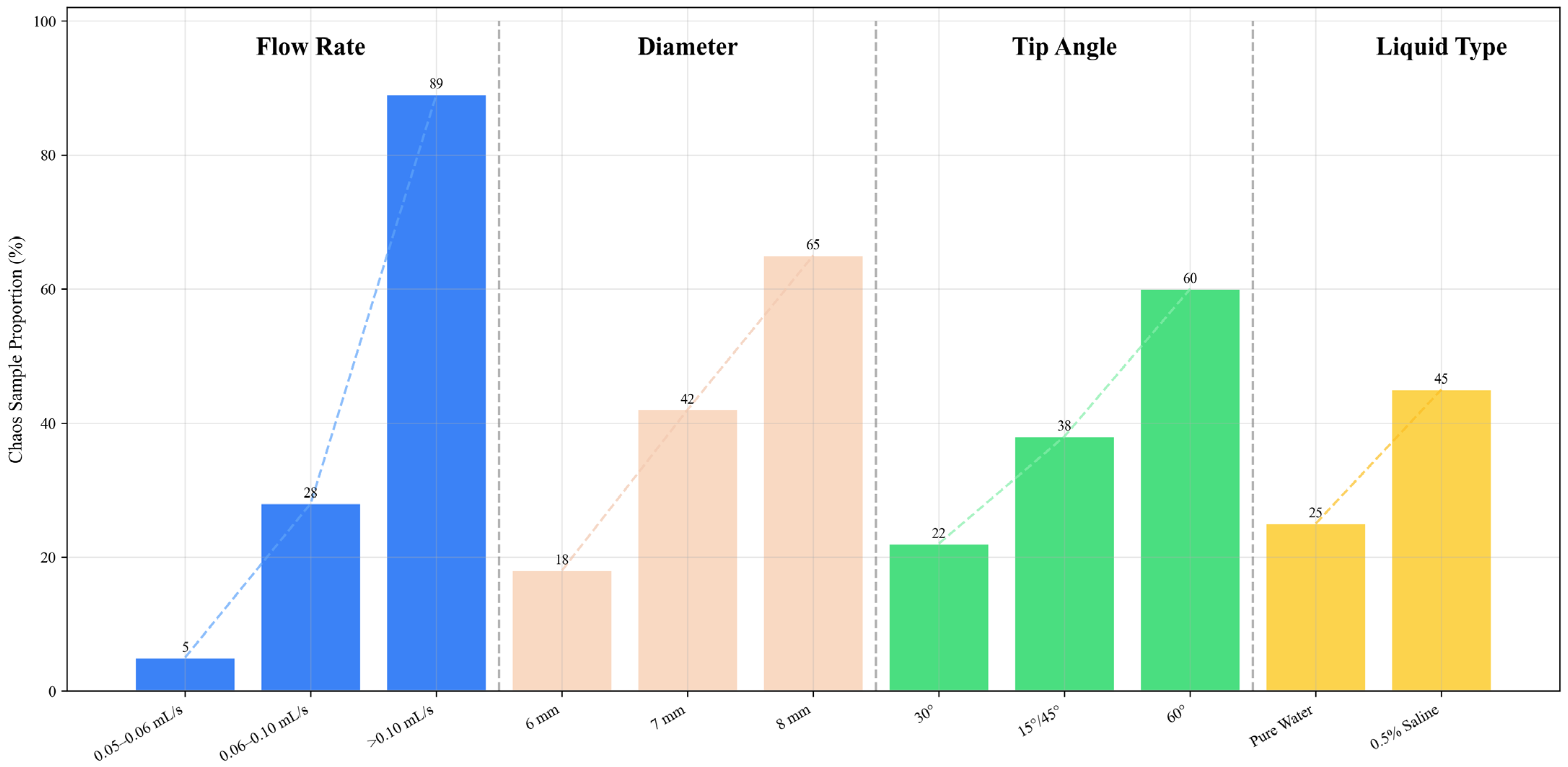
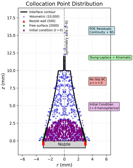
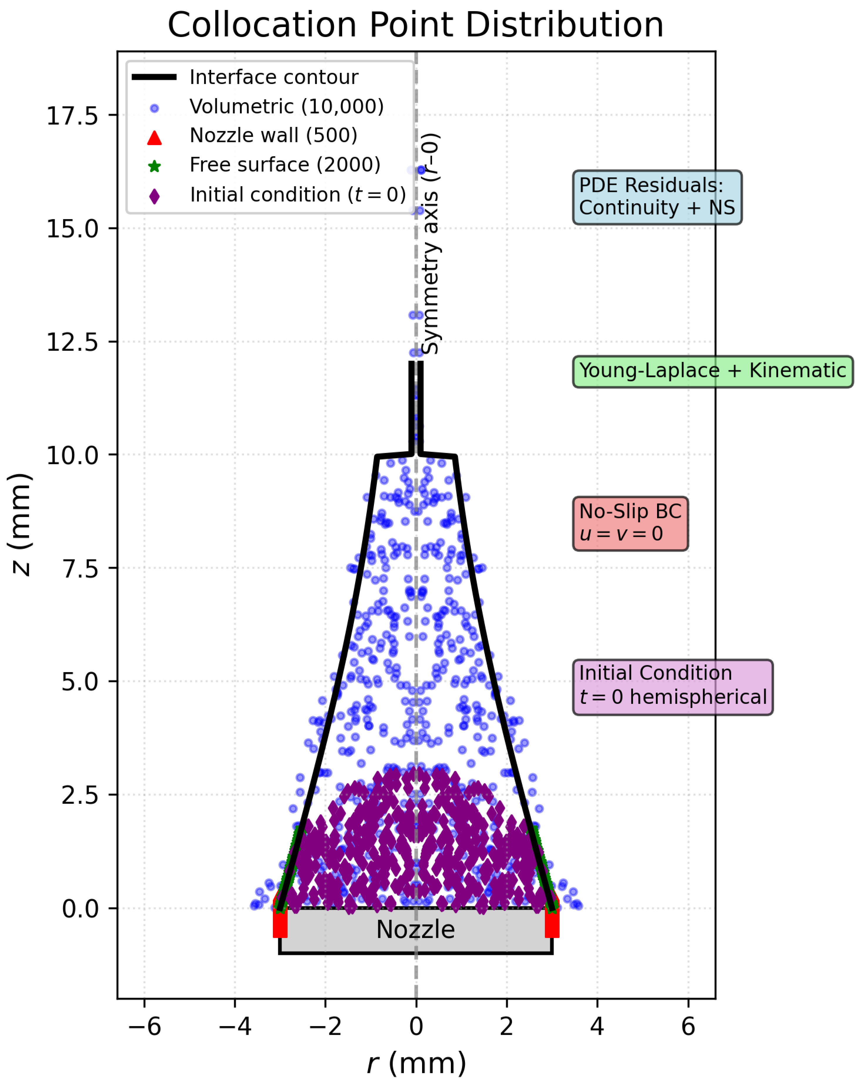
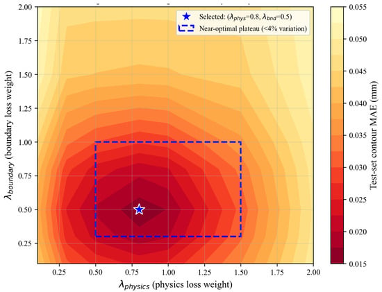
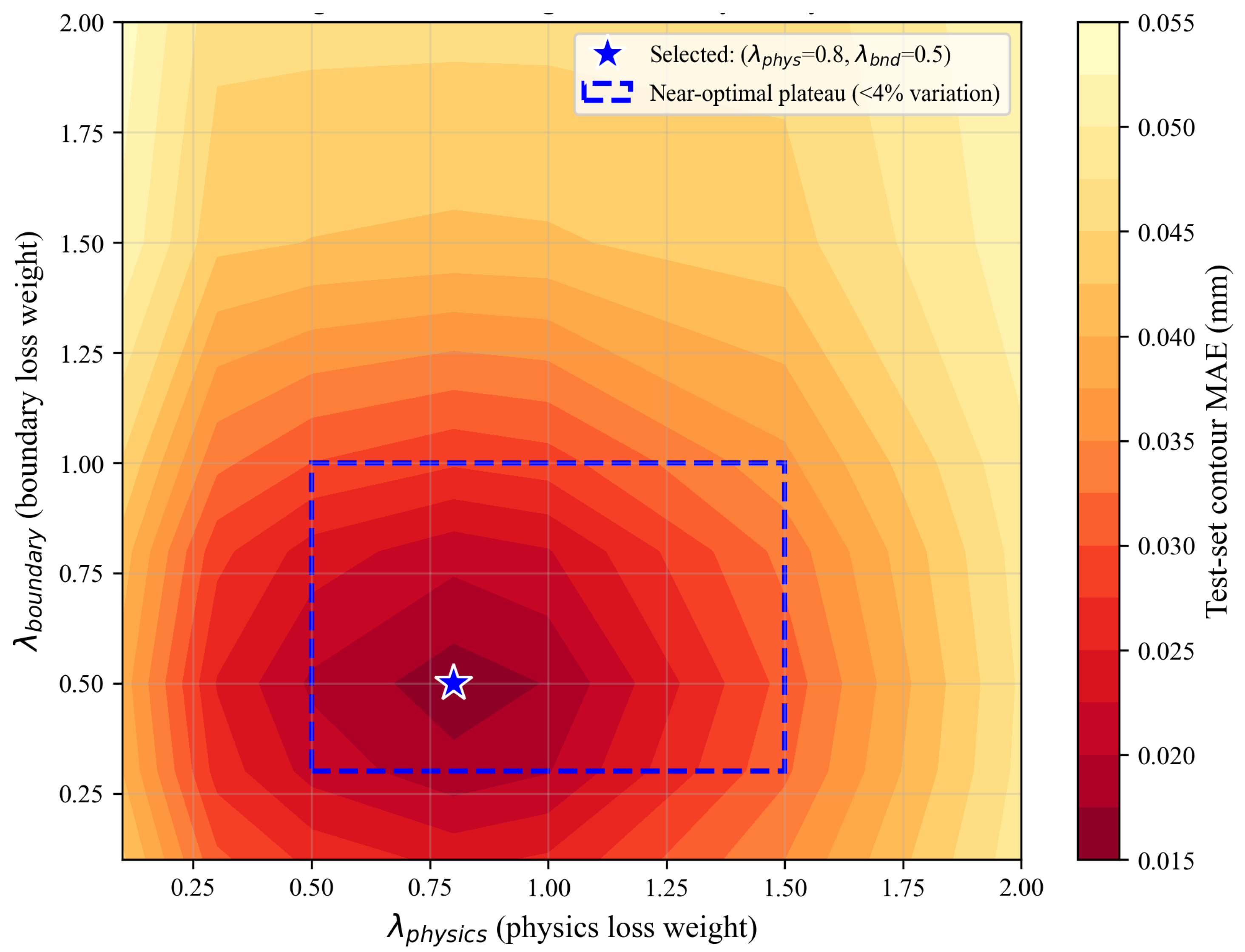
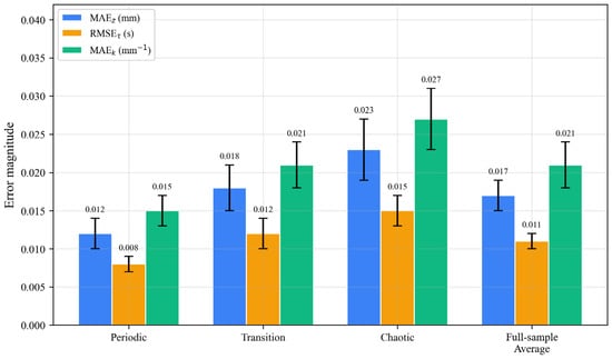
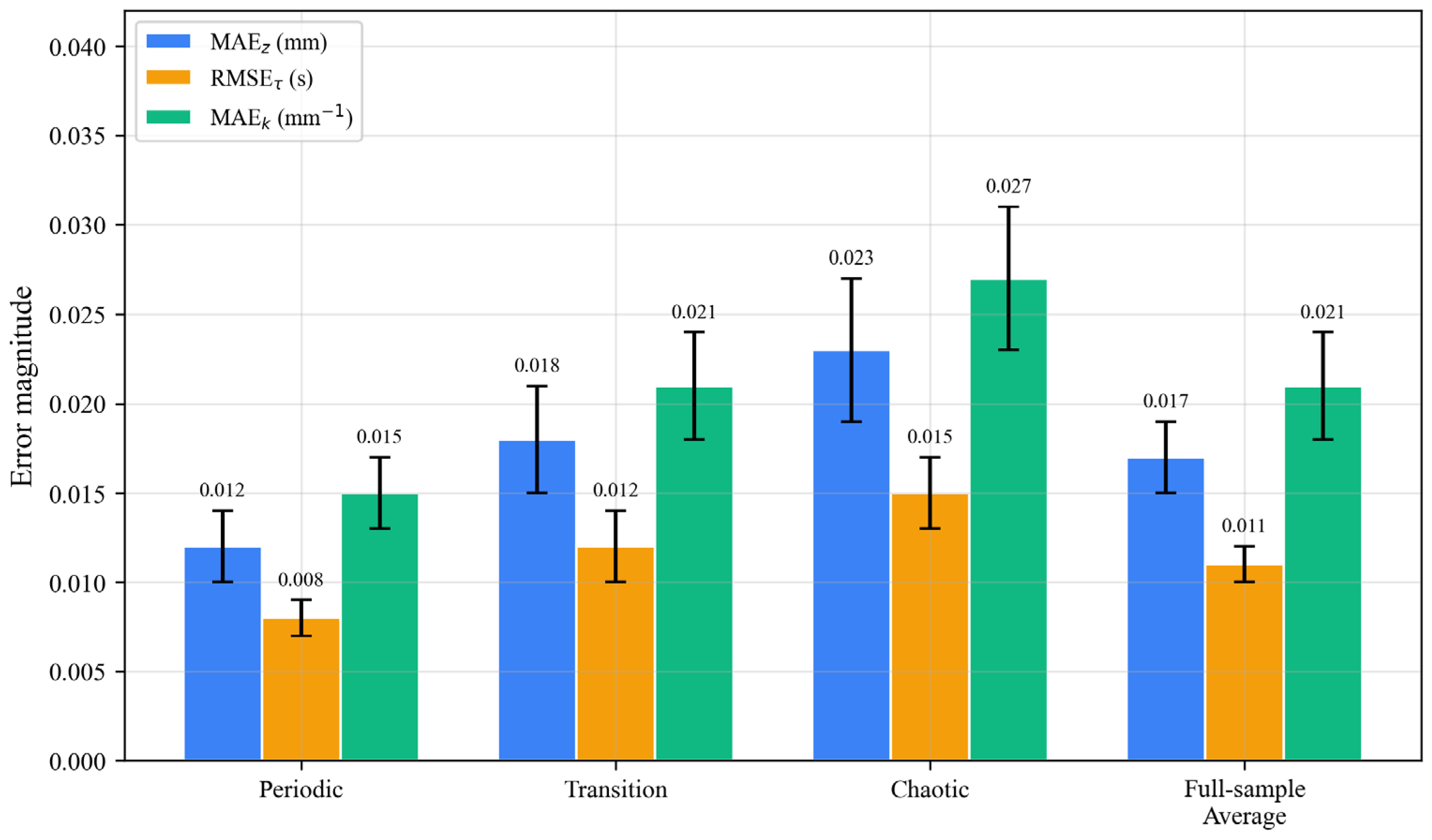
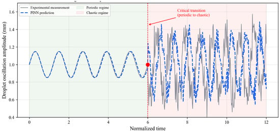
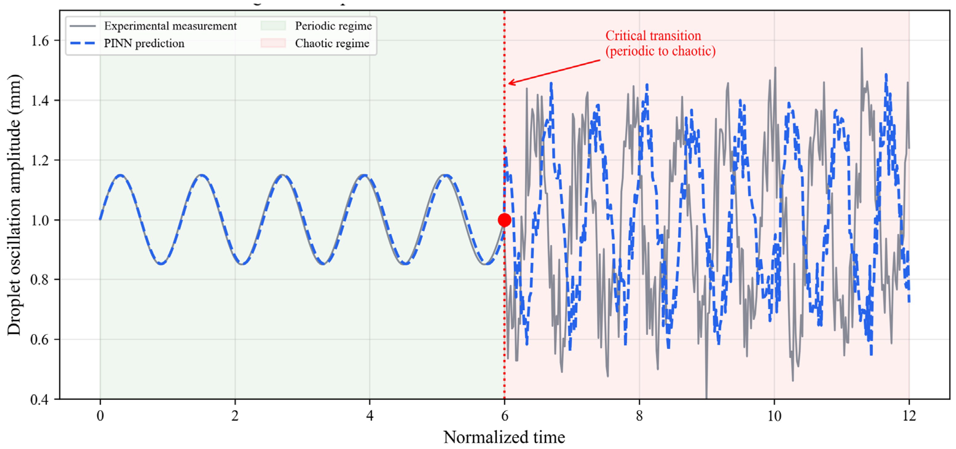
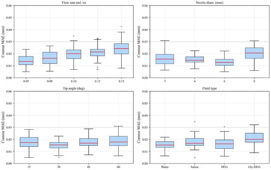
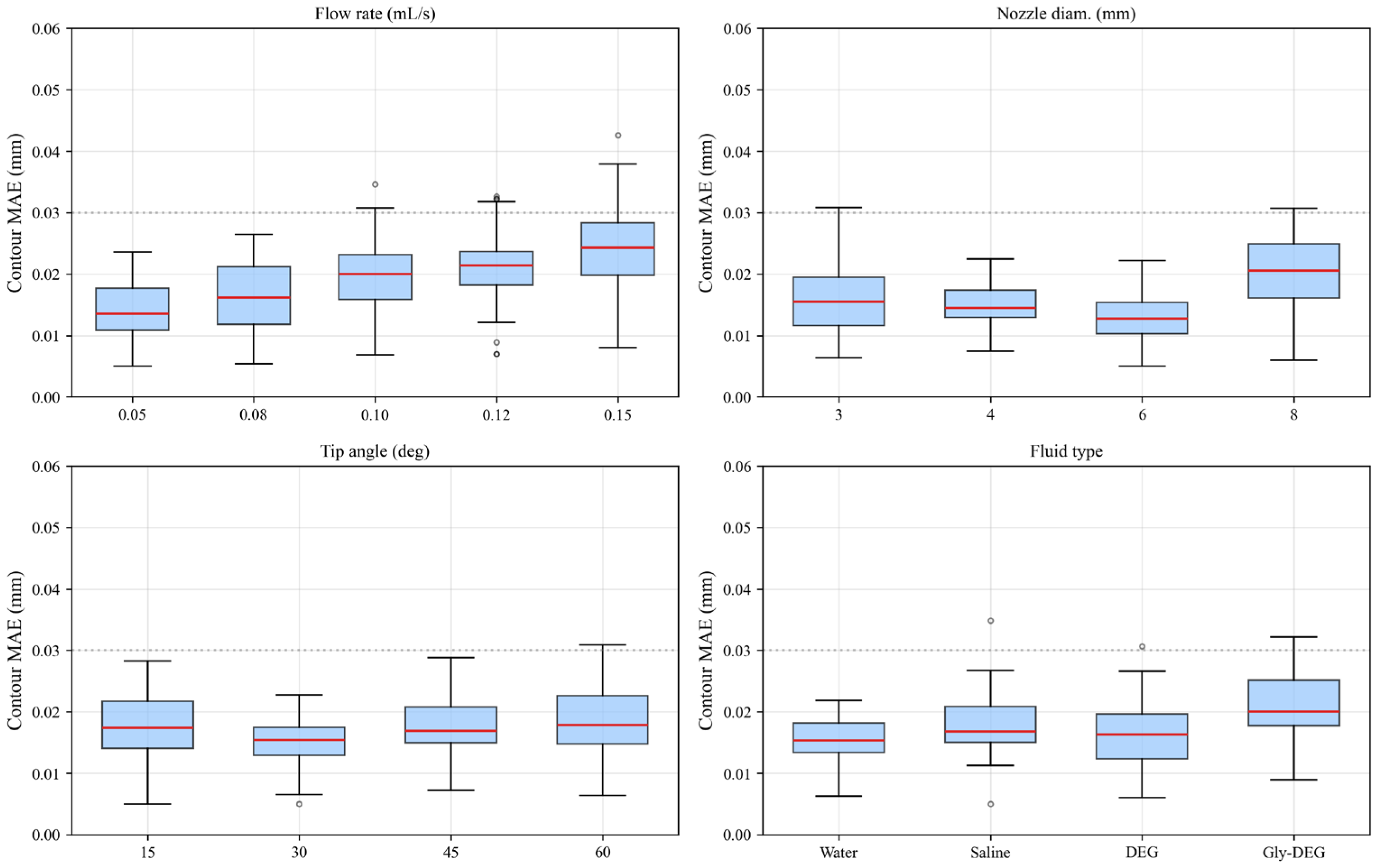
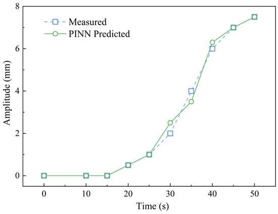
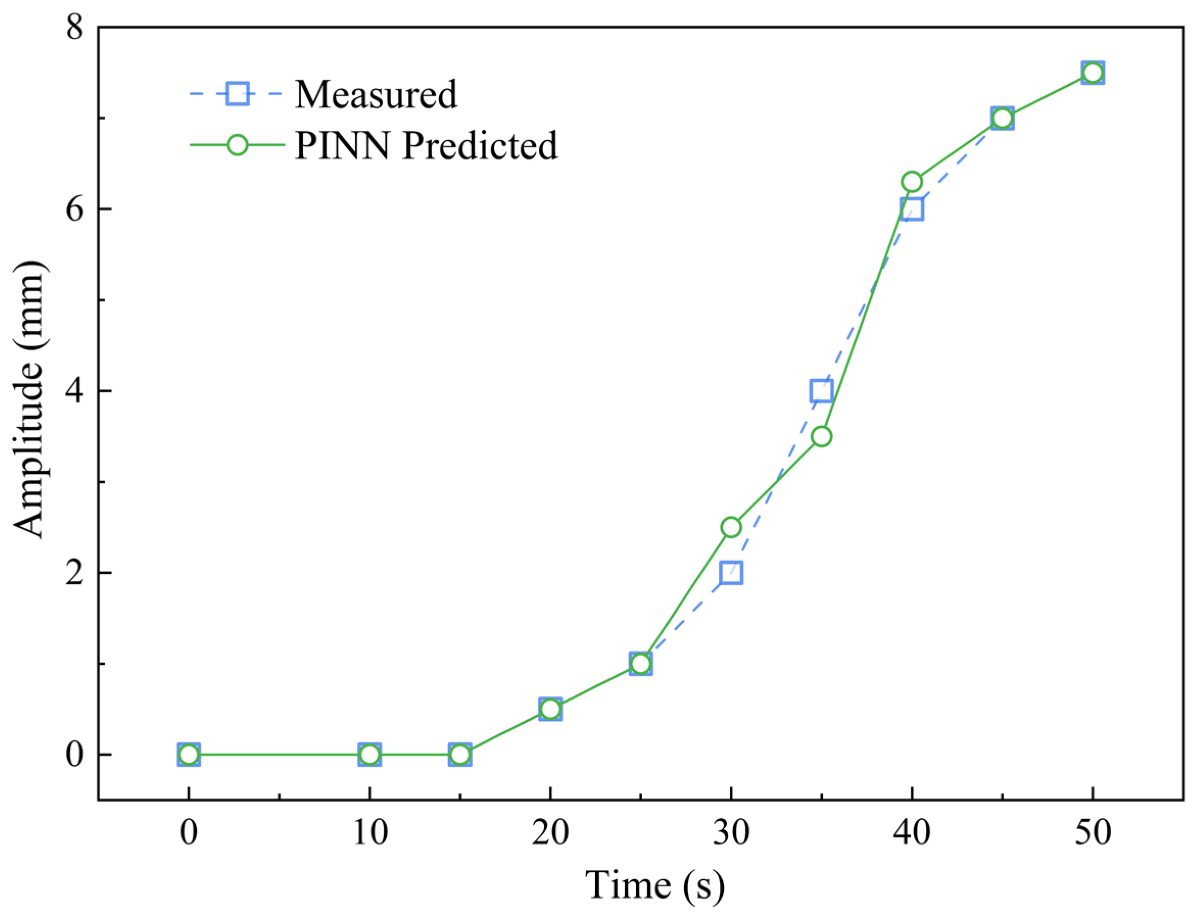
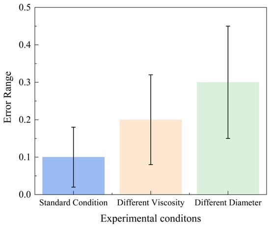
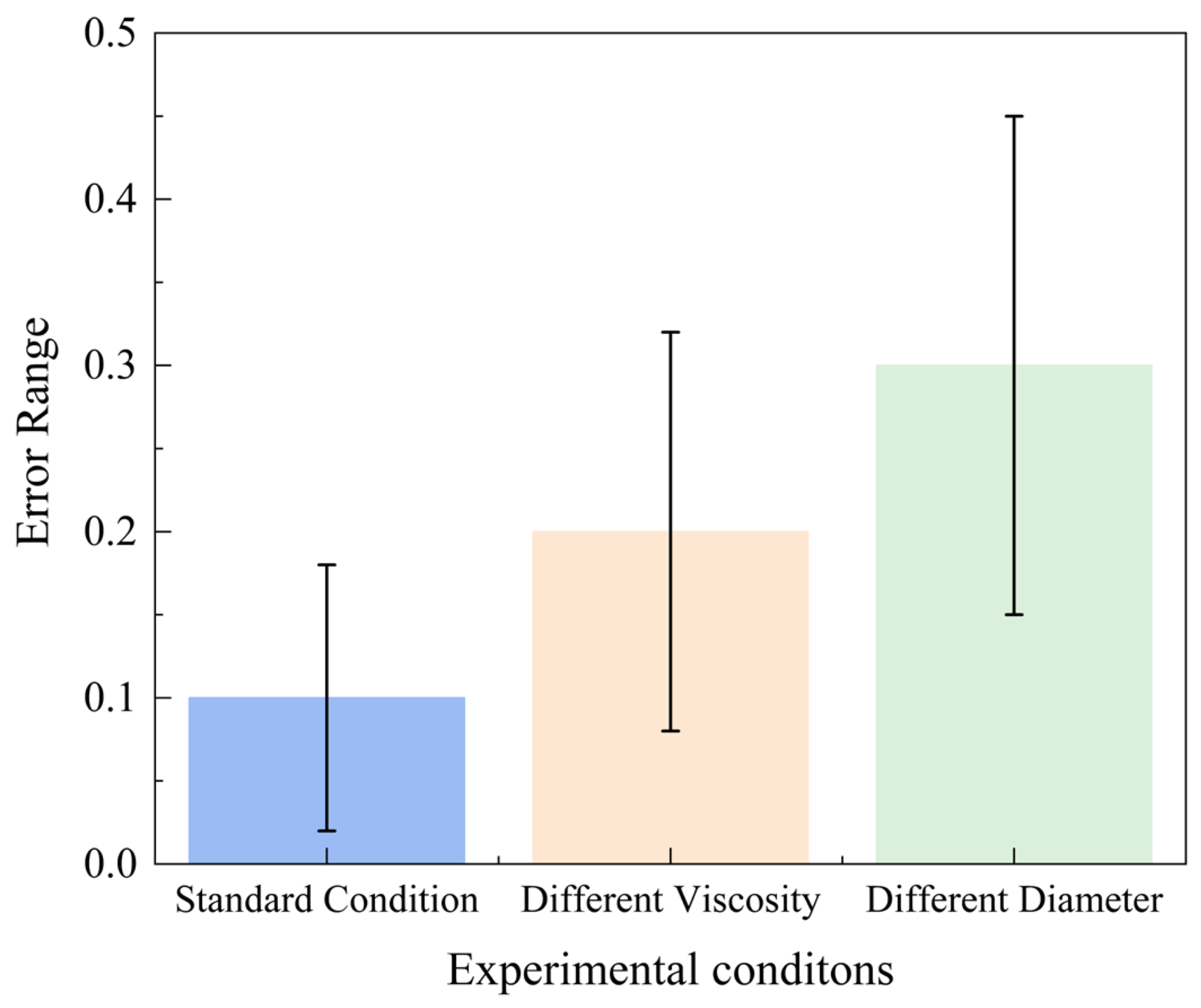
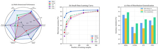
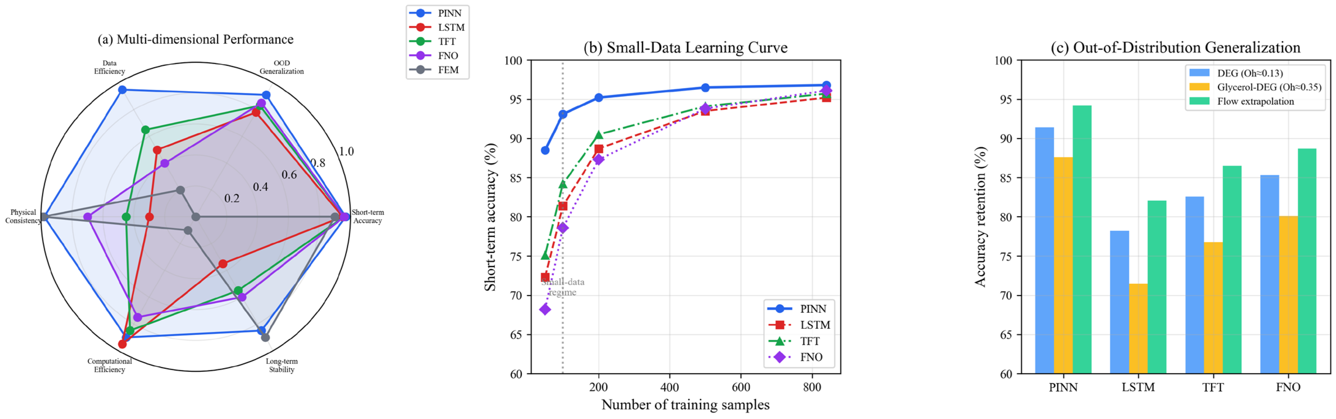
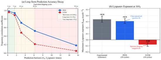
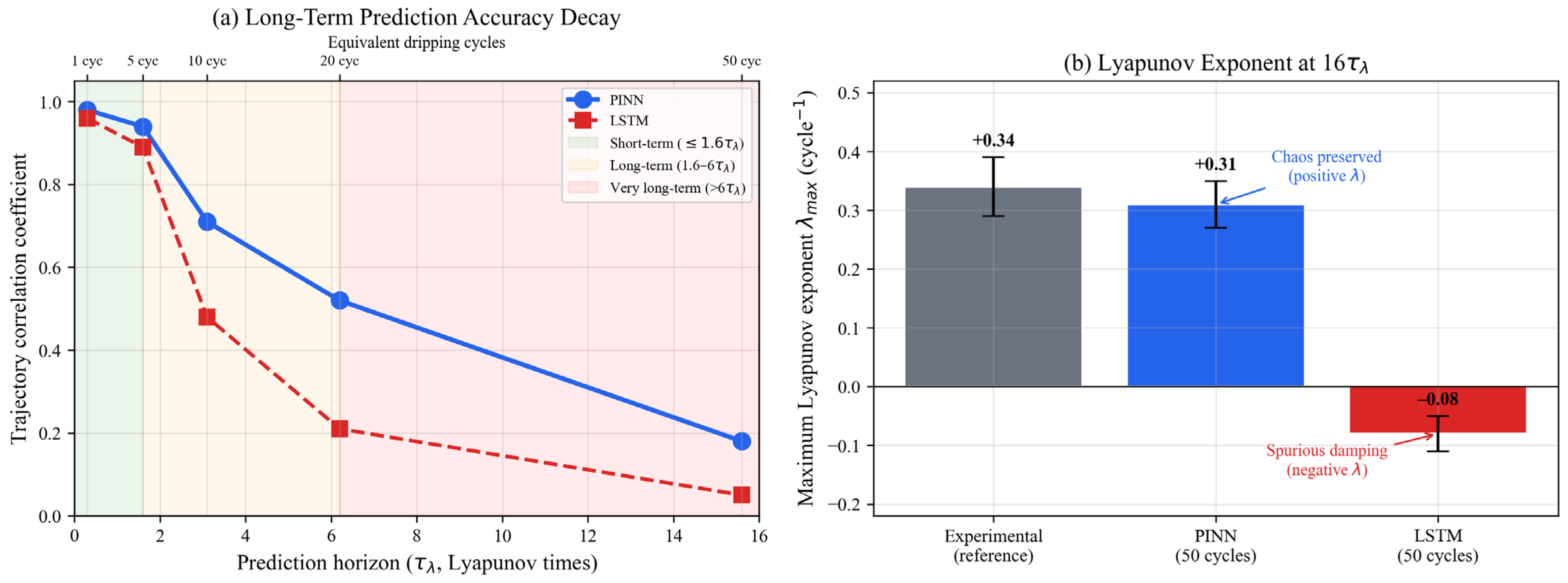
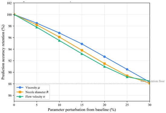
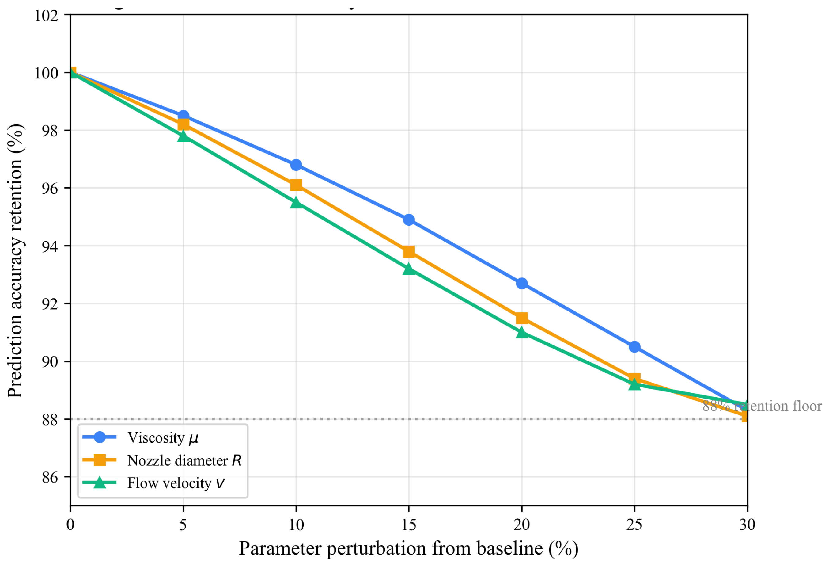
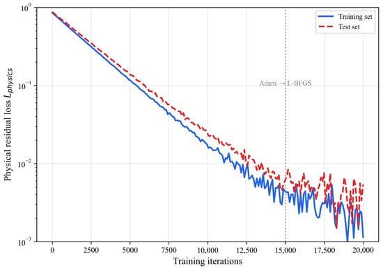
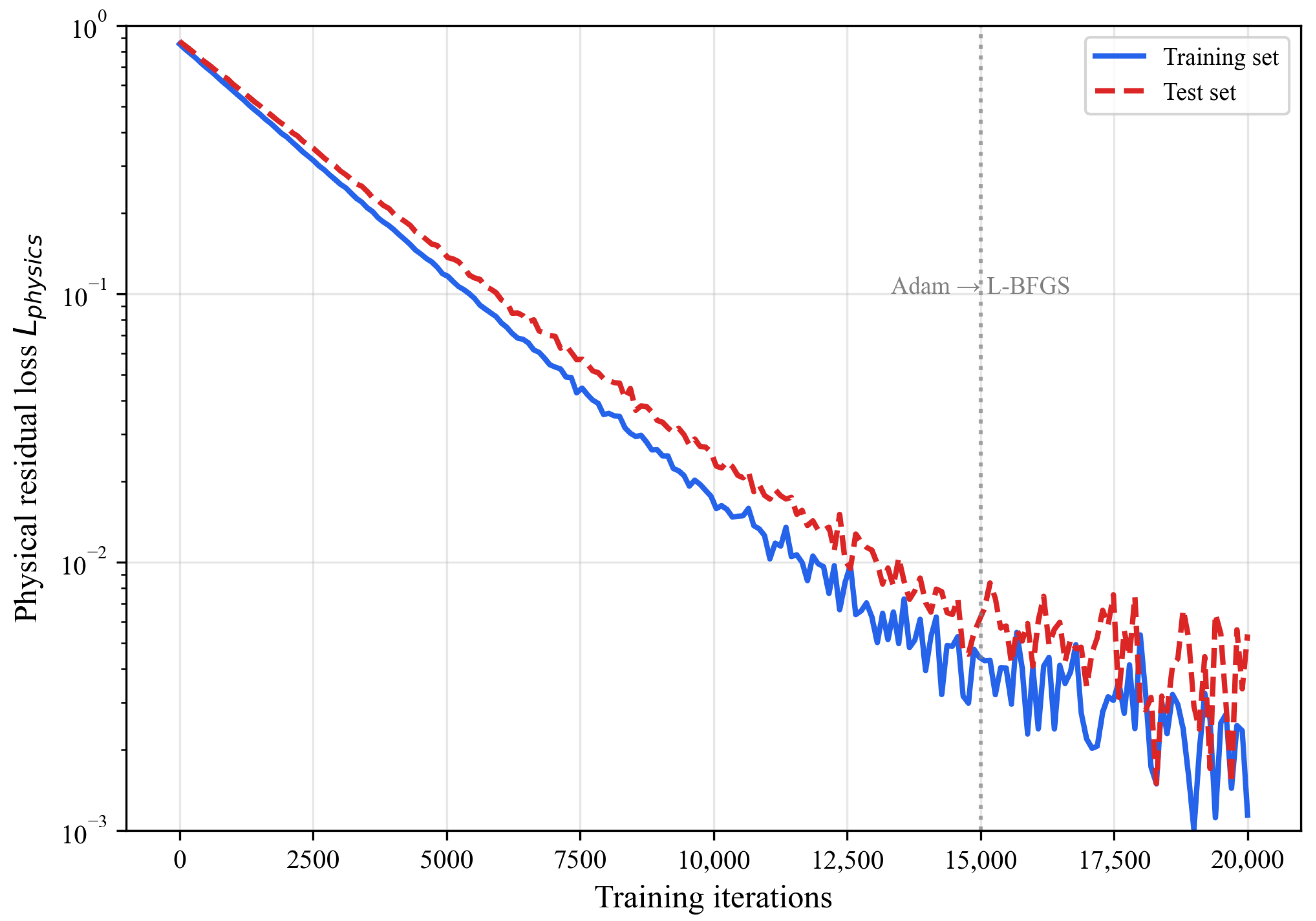
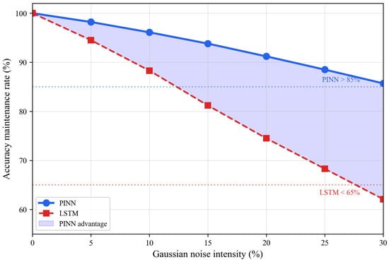
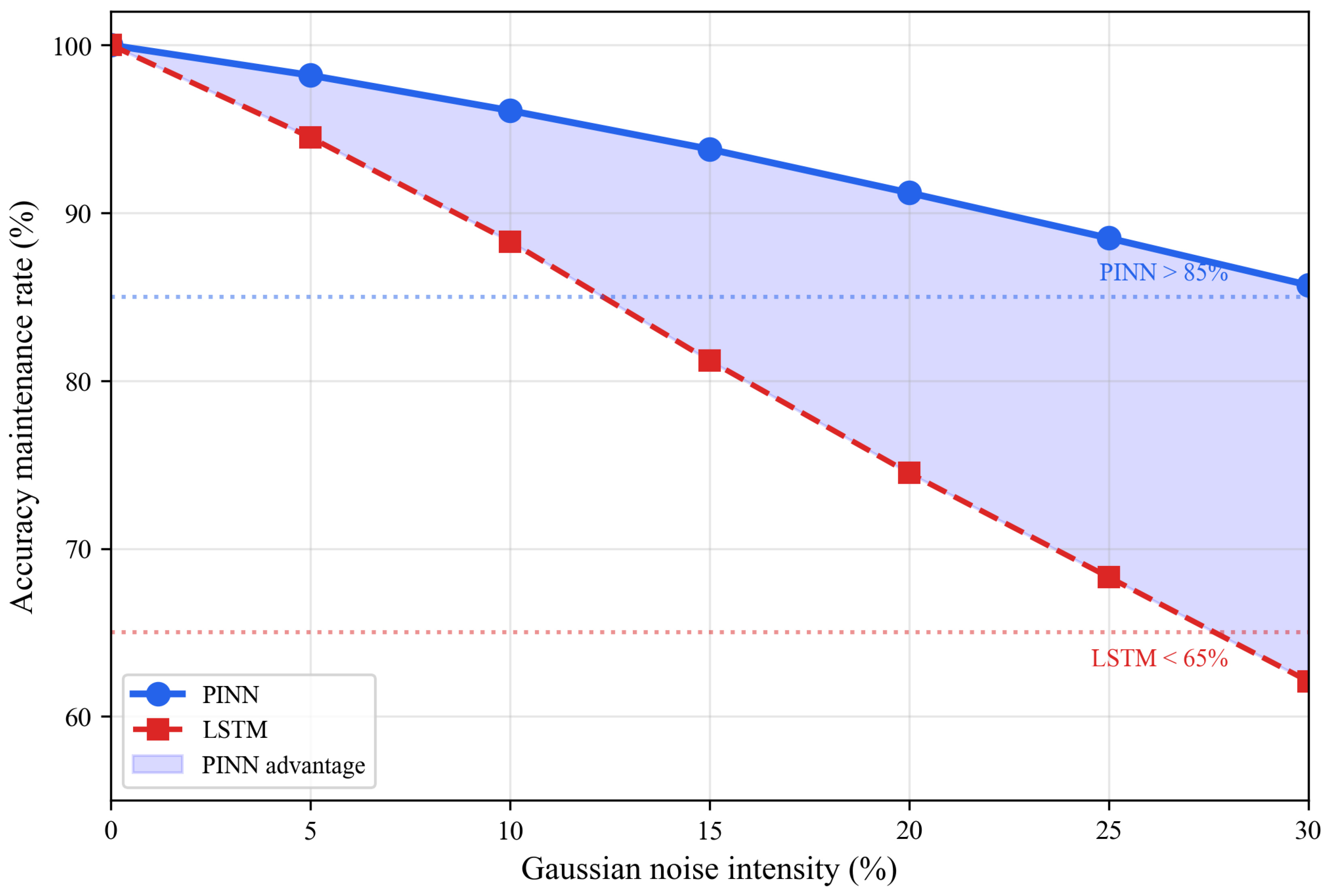

Disclaimer/Publisher’s Note: The statements, opinions and data contained in all publications are solely those of the individual author(s) and contributor(s) and not of MDPI and/or the editor(s). MDPI and/or the editor(s) disclaim responsibility for any injury to people or property resulting from any ideas, methods, instructions or products referred to in the content. |
© 2026 by the authors. Licensee MDPI, Basel, Switzerland. This article is an open access article distributed under the terms and conditions of the Creative Commons Attribution (CC BY) license.