


Abstract
Fully compressible two-phase flow configurations present many challenges for numerical modelling, requiring the development of Real Fluid Models (RFMs) able to simulate flows in subcritical, transcritical and supercritical regimes. Such an RFM has been recently developed at IFPEN based on physical properties lookup tables, mainly for binary and ternary chemical systems. This paper proposes an Artificial Neural Network (ANN) approach to overcome the limitations of lookup tables of thermodynamic properties and to apply RFM to multi-species combustion. A methodology for generating an optimized data set by combining a vapor–liquid equilibrium (VLE) thermodynamic solver and the in situ adaptive tabulation (ISAT) method is developed. It aims to improve the neural network training process for two-phase combustion simulations where many species are present. This ANN methodology has been implemented in the CONVERGE CFD solver and validated using a mixing layer (LOX/GH2) benchmark from the literature relevant to rocket conditions, and an academic gaseous (H2/O2) case relevant to hydrogen combustion. The results show that this ANN approach makes H2 combustion simulation possible when coupled to the RFM framework and using a 10-species kinetic mechanism.
Keywords:
neural network; ISAT; subcritical; supercritical; transcritical flow; real fluid model; VLE; combustion 1. Introduction
Today, injection and combustion of liquid and gaseous fuels such as hydrogen (H2), ammonia (NH3) and (CH4) at supercritical pressures is a frequently used technique to improve the efficiency of energy systems and address environmental constraints. This requires the development of fully compressible two-phase flow solvers able to simulate flows simultaneously in subcritical, transcritical and supercritical regimes. This article focuses on the extension of the IFPEN’s Real Fluid Model (RFM) [1,2,3,4,5] to high-fidelity simulations of multi-component two-phase combustion. In principle, the use of the RFM framework for the computation of the required physical properties in a CFD solver can be done through different methods such as direct coupling to vapor–liquid equilibrium (VLE) solvers, lookup tabulation, or using an Artificial Neural Network (ANN) model. Direct VLE coupling method can be very expensive in terms of CPU cost [1,2], while tabulation may require large memory allocations, making the RFM framework difficult to apply to combustion, for instance, as the number of chemical species increases. ANNs have emerged as a highly effective technique for classification and response prediction, surpassing traditional linear methods like regression analysis. Their superior prediction abilities have been extensively demonstrated, leading to successful applications in various domains of engineering and science [6,7,8,9]. Indeed, there are already numerous attempts in the literature to solve similar problems using ANNs. A comprehensive exploration of the integration of ANN models within the RFM approach for efficiently simulating complex thermodynamic functions in CFD code for a non-evaporating binary mixture under transcritical conditions has been carried out in [8]. This work has highlighted the vast potential of ANNs in the field of multiphase flow and suggests numerous avenues for further extending their application to multi-component systems. More recently, a computational framework that integrates ANN with in situ adaptive tabulation (ISAT) to accelerate and stabilize VLE modeling within CFD simulations has been proposed by [7].
It has been already demonstrated in a previous communication [6,8,9] that ANNs are suitable and efficient for CFD simulation of the cryogenic LOX/GH2 mixing layer in the RFM framework.
In this work, an improved ANN method, capable of handling dozens of chemical species and radicals produced during combustion, is proposed. A key challenge is the generation of a thermodynamic database that enables a fine-tuned description of the neural networks. As with all ANN training processes, the dataset is the most critical input and must be carefully selected. To accomplish this, an ISAT-based sorting tree [7,10] has been employed. In this study, the proposed RFM-ANN model is applied to the CFD simulation of gas combustion (H2/O2) in a 0D-like case using a 10-species mechanism. The paper is structured as follows: Section 2 provides a brief overview of the equations governing the RFM. Section 3 details the database generation process using ISAT. Section 4 presents the ANN design methods. Then, two validation cases have been simulated. Section 5 includes the comparison of different results obtained by the CFD simulation of a mixing layer of a binary (LOX/GH2/) 2D benchmark case proposed by [11]. Finally, Section 6 discusses the results of gaseous (H2/O2) combustion simulations, followed by the conclusions in Section 7.
2. The RFM Governing Equations
The diffused interface two-phase flow model adopted in the current work is a four-equation model that is fully compressible and considers multi-component in both phases under the assumptions of thermal and mechanical equilibrium as follows:
where is the viscous stress tensor, is the density, is the velocity, is the pressure, is the specific internal energy, and is the temperature. In addition, are the mass fraction and specific enthalpy of species , respectively. The thermal conductivity and the dynamic viscosity cover laminar and turbulent contributions. The laminar contribution of is computed by Chung et al. [12] correlations. The turbulent conductivity is calculated using a given turbulent Prandtl number and the turbulent viscosity is given by the adopted turbulence model. The laminar and turbulent mass diffusion coefficients are estimated using a given Schmidt number. Finally, and are respectively the species and energy chemical source terms provided by the kinetics solver SAGE in CONVERGE v4.1 (see Section I.2 in [13] for discussion on combustion modeling).
Originally, for binary or ternary systems, the RFM is closed by a thermodynamic equilibrium tabulation method [3,4,5]. The thermodynamic table is generated using the in-house IFPEN CARNOT library [5] based on VLE calculations coupled with a real-fluid equation of state (EoS), such as Peng–Robinson (PR-EoS) and Soave–Redlich–Kwong (SRK-EoS) [4,5]. The thermodynamic and transport properties of the mixture, such as the density , the specific internal energy , the heat capacities (Cp, Cv), the speed of sound (Cs), the thermal conductivity, and the dynamic viscosity are calculated as a function of temperature (T), pressure (P), and mass fraction of the species in the mixture (Yk), and stored into a table.
In addition, the RFM has initially employed a lookup procedure using a multilinear interpolation on a regularly structured discretization of temperature, pressure and mass fractions [5]. However, for cases involving more than three species, the size of the generated table became prohibitively large, leading to excessive memory consumption and computational overhead. To overcome these limitations, an Artificial Neural Network (ANN)-based methodology is proposed as an alternative to the traditional tabulation approach. This ANN framework should enable efficient and scalable CFD combustion simulations, even for cases involving a large number of species, by significantly reducing storage requirements while maintaining the thermodynamic and transport properties accuracy, and computational robustness and efficiency. A typical ANN framework employing an in situ adaptive tabulation (ISAT)-based sorting tree [10] is described in the following sections.
3. Data Base Generation Using an ISAT Method
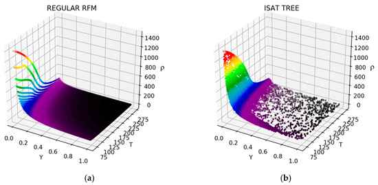
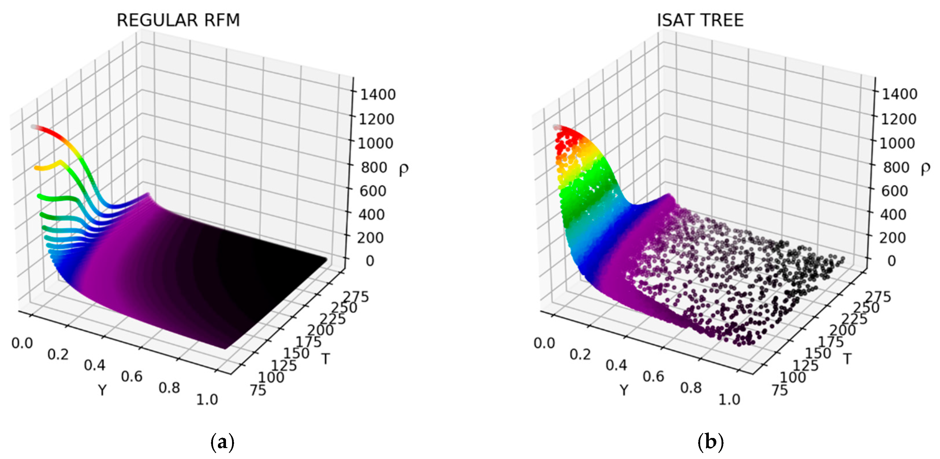
To generate the database for the initial binary (O2/H2) system of interest in this study, CARNOT v10.9 [14] was first used to generate a structured regular table for the system (O2/H2) in the same way as for the tabulation method used previously in [5], for instance. The density in the plane P = 105 bar of this regular database is depicted in Figure 1a. It can be observed in this figure that many points describe the same vapor density solution, and that in areas where density increases rapidly (near to liquid–vapor phase boundary), the description will be fragmentary and less refined. We therefore need to adopt a physically more appropriate strategy for generating training databases. The proposed new strategy is based on the use of the ISAT method [10] to optimize the size of the database and identify and better refine high-gradient density regions, as shown in Figure 1b. This method has the advantage of being able to sort the data on the fly in a binary tree construction.
Figure 1.
(a) Regular data generation vs. (b) ISAT data generation (isobar scatterplot for P = 105 bar). (ρ) is the mixture density colored by its magnitude, Y the mass fraction of H2.
The function used for the ISAT sorting tree may be written as Z = CARNOT(X), where X is the input vector (P, T, Yk) and Z is the output vector (ρ, e, Cv, Cp, Cs, λ, μ) obtained using the in-house CARNOT library.
We will set Xmin and Xmax, the lower and upper limits between which the values of X will be tested, this means that we limit the pressure between two minimum and maximum values, and the same applies to temperature and mass fraction. For example, for the case of two species, H2/O2, we have a pressure range of 90–110 bar, a temperature range of 70–270 K, and a H2 mass fraction ranging from 0 to 1.
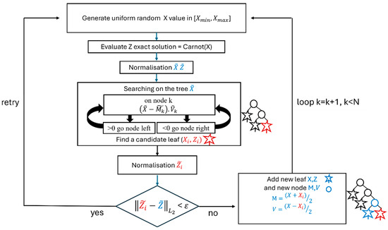
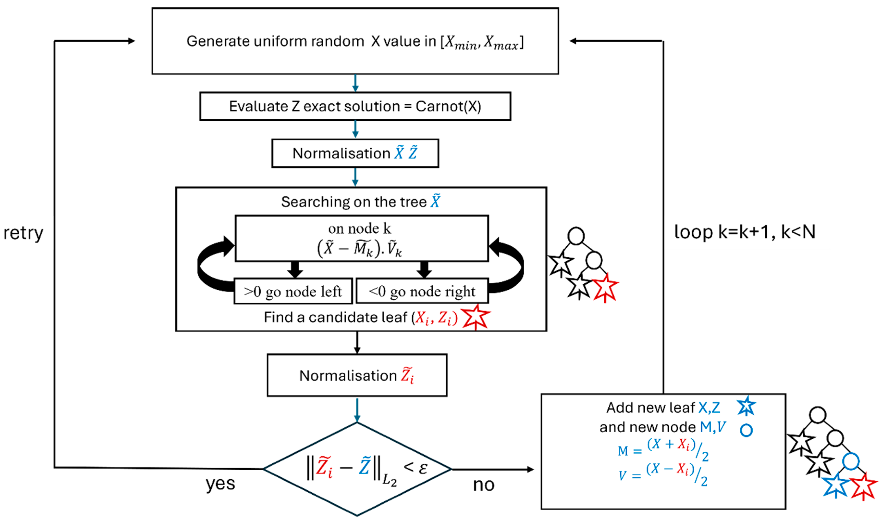
The first step is to normalize X and Z. This normalization involves defining a vector representing an average value, allowing quantities that may not initially be of the same order of magnitude (such as temperature, pressure, and mass fraction, for example) to be combined consistently.
Next, the tree is traversed by performing an elementary scalar product, which determines whether to move to the right or left branch. This process continues until the leaf node closest to X is reached. At this leaf node, the quantities Xᵢ and Zᵢ are retrieved.
The L2-norm difference between the normalized Z and normalized Zᵢ is then computed. If this value is smaller than the ε parameter, the pair (X, Z) is considered redundant and is not added to the database. Otherwise, the pair is deemed relevant and stored in a new leaf. When a new leaf is created, the previously found leaf (, ) is moved and both leaves are connected through a node storing the midpoint M = (X + Xi)/2 is stored along with a vector V = (X − Xi)/2 (which will facilitate traversal down the tree via the dot product, see Figure 2).
Figure 2.
ISAT procedure to sort the database.
This process is iterative, and new (X, Z) pairs are generated until a sufficiently large and complete database is obtained. In practice, between 5 and 10 million input values are tested, with only about 10% of the data retained using this method, in order to obtain a representative sampling of the fluid behavior.
Note that normalizing the Z components is essential for properly sorting the Z values. For example, by reducing the normalizing factor such that , the discretization of is refined. This is a key aspect for achieving a more reliable neural network capable of making finer predictions (see Figure 1).
Therefore, by using such an ISAT method, one can immediately observe in Figure 1 that the density (ρ) is described with higher resolution in regions of large gradient values, whereas flatter regions (plateaux) require fewer data points in the sorted database. In this context, the number of points required to define the training database was reduced by more than 50%, from 1,030,301 points which is (101 × 101 × 101) points in the regular database to 557,277 points in the ISAT-sorted database.
4. Artificial Neural Network Generation
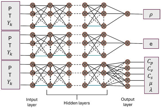
The architecture of the ANN model was systematically optimized using the OPTUNA software v3.3.0 (see [15] for example). This powerful hyperparameter optimization tool allowed us to explore a wide range of network configurations and identify the most suitable architecture for our specific problem. By leveraging OPTUNA’s automated search capabilities, we were able to fine-tune key parameters such as the number of layers, the number of neurons per layer, the activation functions, and the learning rate. This approach ensured that our ANN models achieved optimal performance while maintaining computational efficiency. Initially, we employed a single ANN model to predict various thermodynamic properties, required by computational fluid dynamics (CFD) simulations. While this approach proved successful for certain parameters, it was insufficient for others, particularly density (ρ) and specific internal energy (e). These two parameters play a crucial role in ensuring numerical stability and convergence in CFD simulations as they are closely related to mass and energy conservation (see Equations (1) and (3)), making their accurate prediction essential.
The limitations of the single ANN model led us to explore alternative strategies to enhance the predictive capabilities of our neural network framework. To facilitate the development of a more robust neural model, we implemented a hybrid solver capable of running both the RFM tabulation model and the RFM-ANN model simultaneously. This hybrid approach allowed us to systematically assess and control the error introduced by the ANN predictions in the CFD computations. By comparing ANN-generated results with those obtained using the tabulation model, we were able to identify discrepancies and redefine our ANN accordingly. This validation step was critical in ensuring that the ANN models did not introduce numerical errors that could compromise the accuracy of the CFD simulations. Through extensive error analysis, we realized that a single ANN structure was unable to provide uniformly high accuracy across all target parameters. Some properties exhibited higher sensitivity to neural network approximations, which led to greater discrepancies in their predicted values, followed by the CFD solver crash. As a result, we determined that it was more effective to decompose the ANN output space into three distinct sets, each handled by a separate neural network. This multi-network approach allowed for specialized training and optimization of each ANN, ensuring that the predictions remained as accurate as possible while maintaining computational efficiency. Dividing the outputs into three separate networks not only reduced overall prediction errors but also enhanced the stability and robustness of CFD simulations, leading to better numerical convergence. This multi-network methodology highlights the importance of tailoring ANN architectures to the specific requirements of CFD applications, ensuring both accuracy and computational efficiency in large-scale simulations.
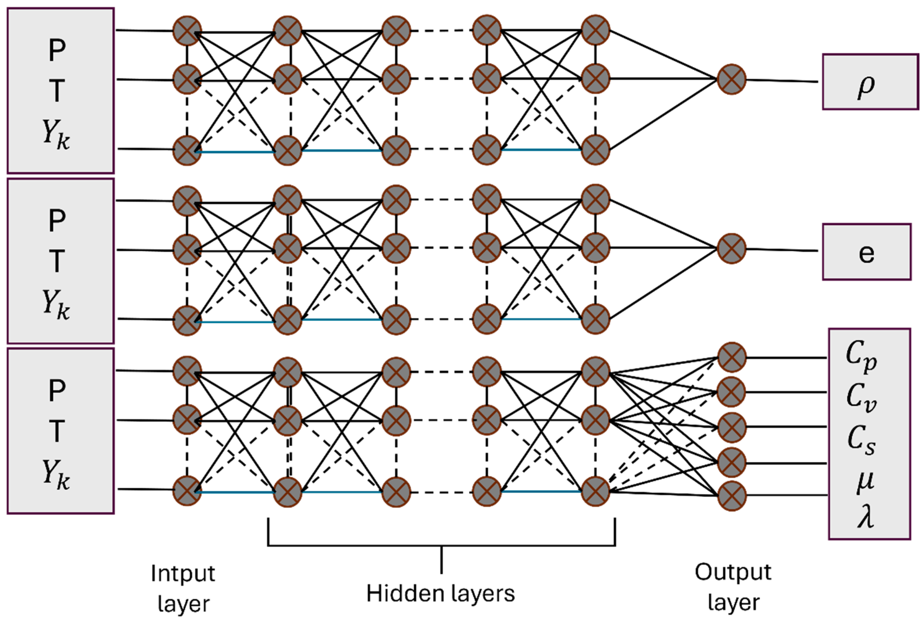
Thus, the first two ANNs are dedicated to predicting the two most critical parameters for CFD simulations: density (ρ) and specific internal energy (e), as depicted in Figure 3. These physical properties are essential for ensuring numerical stability and convergence, making their accurate estimation a priority, as their conservation is required by Equations (1) and (3). The third neural network is responsible for predicting the remaining thermodynamic (Cv, Cp, Cs), and transport properties (λ, μ), as illustrated schematically in Figure 3. By allocating separate networks to different parameter groups, we optimized each ANN’s learning process to focus on a specific subset of variables. This specialization allowed for more precise predictions, as each network could be fine-tuned to the unique characteristics and sensitivities of its respective parameters. Moreover, this multi-network approach helped mitigate potential sources of numerical error that may arise when attempting to train a single ANN to handle a wide range of parameters with varying degrees of complexity. The tailored structure improved generalization across different CFD conditions while maintaining computational efficiency, ultimately leading to more reliable and stable simulation outcomes.
Figure 3.
Multi-network optimized ANN design using three dedicated models for the density (ρ), specific internal energy (e) and all other properties.
For training the neural networks, the mean squared error (MSE) is used as the loss metric. Training is performed sequentially for 1000 epochs, followed by batch training for 3000 epochs. The training is carried out on a single computing node of the supercomputer (2 × 64 cores, AMD Genoa 9534, Advanced Micro Devices, Inc. (AMD), Santa Clara, CA, USA) using TensorFlow v2.15.
5. LOX/GH2 Shear Layer Benchmark
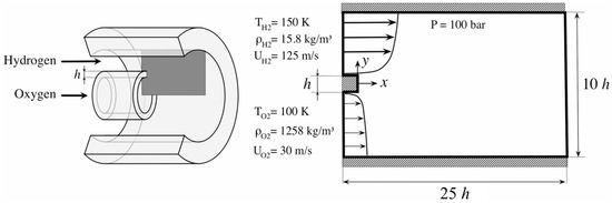
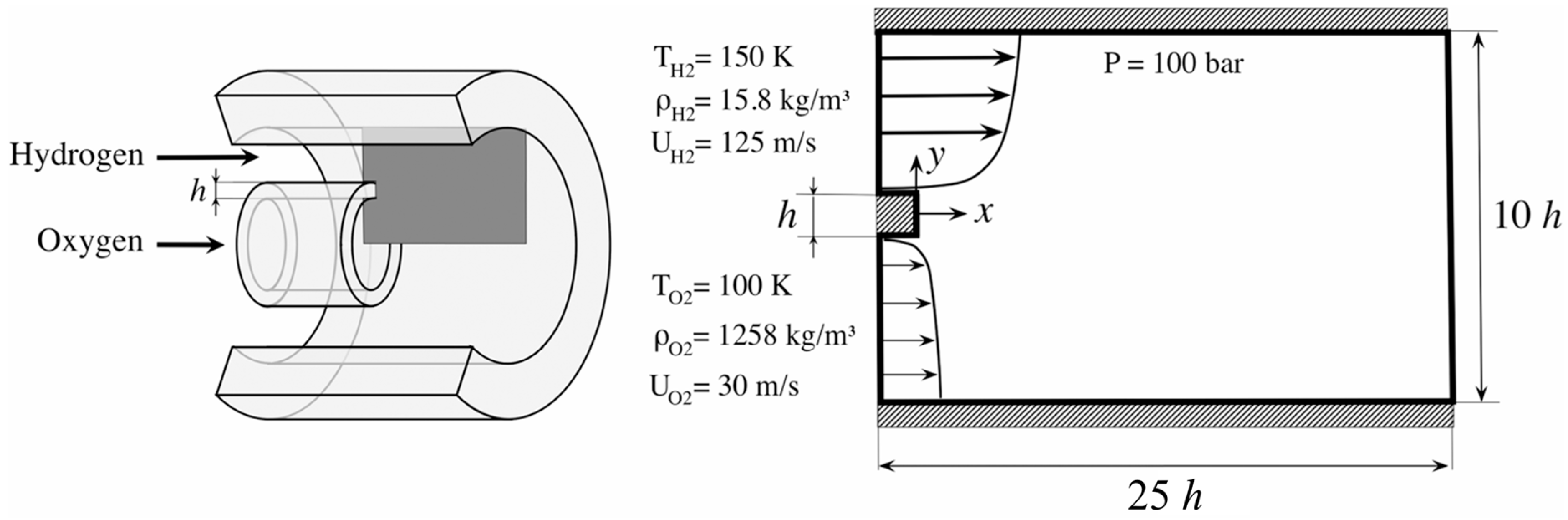
In this section, we present the validation of the proposed ANN methodology based on the CFD simulation of a binary (LOX/GH2) shear layer benchmark proposed by [11]. The boundary conditions and the computational domain are shown in Figure 4. The thermodynamic and injection conditions are realistic in relation to actual rocket devices. No velocity fluctuation is imposed on the inlet planes, and the velocity profiles follow a (1/7)-power law. Initially, these profiles are mapped along the whole computational domain. The nozzle lip separator is represented by an adiabatic wall condition. Static pressure is imposed at the outlet without any sponge layer. The upper and lower limits of the two-dimensional (2D) domain are given symmetry boundary conditions.
Figure 4.
LOX/GH2 shear layer benchmark. (Left) Zoom on the nozzle highlighting the 2D computational domain. (Right) Computational domain with boundary and initial conditions. This figure is adapted from [11].
As a first approach, we used an RFM tabulation of thermodynamic and transport properties and compared the simulation results with those obtained using the proposed ANN.
For the ANN methodology, we used two approaches: the first involved training neural networks using regular tabulation as a database, and for the second, we used the optimized database resulting from ISAT sorting, as illustrated in Figure 1. We used the OPTUNA tool to define the architecture and the size the neural networks as shown in Table 1.
Table 1.
Neural Network description.
An in-house NNICE v1.0 inference tool [16] is used to integrate ANN into the CFD solver. It allows to optimize prediction response times in the context of MLP (multi-layer perceptron) neural networks.
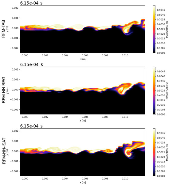
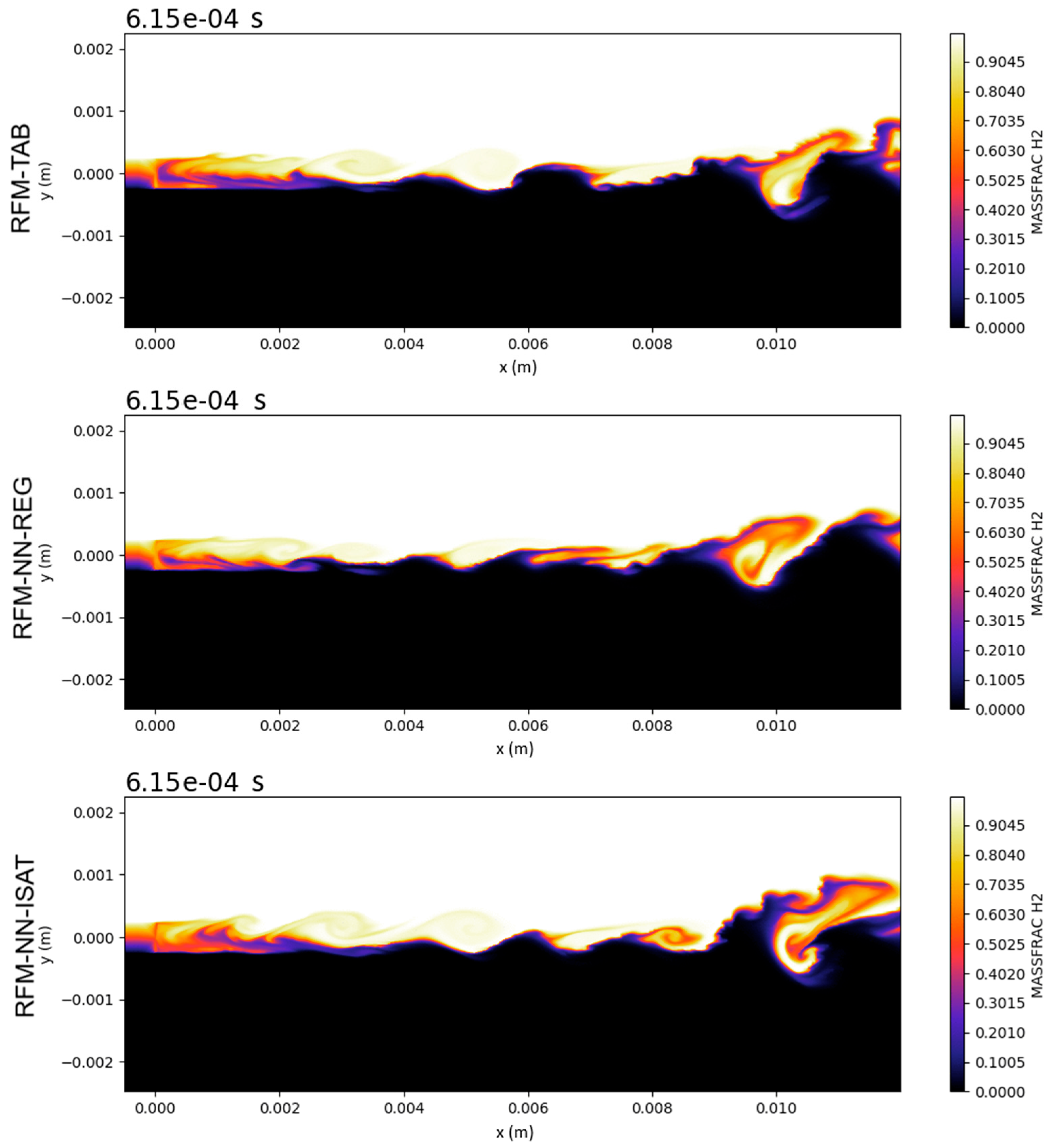
The first results are shown in Figure 5, where we present the H2 mass fraction during the simulation for the three kinds of simulation, RFM-TAB for RFM with regular tabular interpolation, RFM-NN-REG for RFM with Neural Network train with regular table and RFM-NN-ISAT for RFM with Neural Network train with ISAT-generated database.
Figure 5.
LOX/GH2 shear layer benchmark. Instantaneous H2 mass fraction view at t = 615 µs for the three types of simulations: RFM-TAB for RFM with regular tabular interpolation, RFM-NN-REG for RFM with Neural Network train with regular table and RFM-NN-ISAT for RFM with Neural Network train with ISAT-generated database.
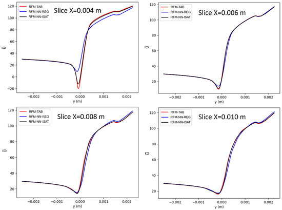
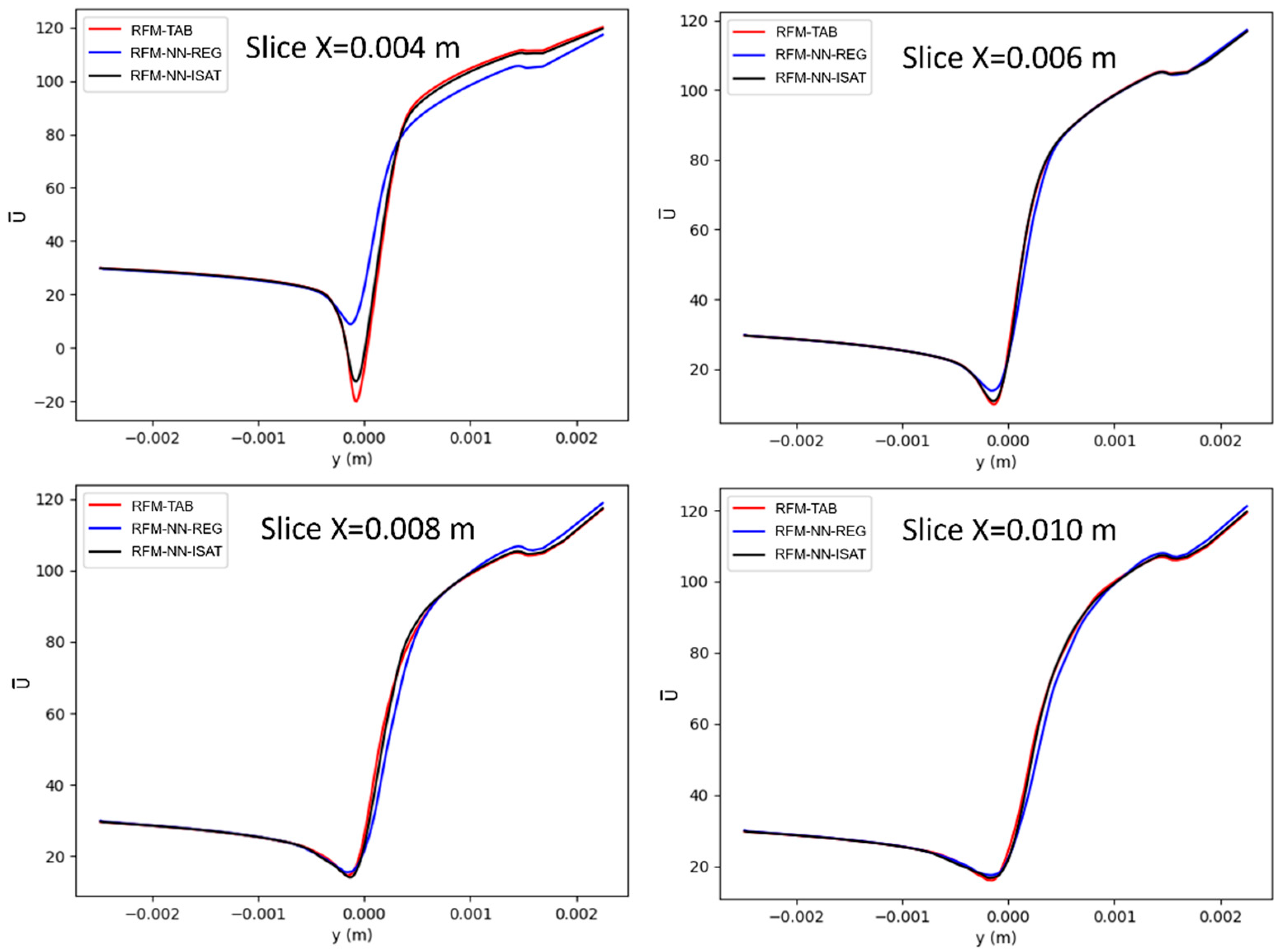
For more detailed comparison purposes, in Figure 6, the velocity U has been averaged over time (denoted ) starting from the middle of the simulation (when the flow had passed through the simulation box between the inlet and outlet several times), for the three kinds of simulation.
Figure 6.
LOX/GH2 shear layer benchmark. Average speed () values obtained by the different approaches in different slices. Refer to Figure 5 for the slice position.
Similar behavior between the reference case, RFM-TAB, and the RFM-NN-ISAT simulation may be noted. This is particularly true for cut plans, but also for snapshot images (see Figure 5 and Figure 6).
We were unable to perform a run with direct coupling to the CARNOT solver (too CPU-intensive), so the reference we consider here is the RFM_TAB run, since here we interpolate the quantities from Carnot directly. Based at Figure 6 ( Slice X = 0.004 m), we observe a good match between the RFM-TAB simulation and the RFM-NN-ISAT simulation, much better than that of RFM-NN-REG, the comparison may seem subjective due to their very similar behavior. It is also important to note that this approach is necessary if we want to include more species to describe the mixture, particularly if we aim to achieve combustion including a high number of species. Indeed, as discussed in the Introduction, for more than three species, it is no longer possible to define a regular table as it would be too large.
This allows us to consider the approach of sorting training data using an ISAT tree structure as a better approach than RFM-NN-REG.
6. H2/O2 Combustion Test Case
To demonstrate the feasibility of a RFM simulation with combustion, the proposed RFM-NN-ISAT is used in this section. To do so, a homogeneous reactor is considered with an initial gas mixture and thermodynamic conditions that allow auto-ignition of the mixture (initial conditions temperature at 1200 K, pressure at 10,325 Pa, , , ). The selected test case is a 0D homogeneous gaseous (H2/O2) mixture, using a detailed 10-species kinetic scheme [17]. As the mixture is homogeneous and quiescent, no turbulence/chemistry interaction takes place. This is why the SAGE detailed chemistry solver available in CONVERGE CFD v4.1 [13] is used to compute reaction rates between H2 and O2 using local conditions and the fundamental principles of chemical kinetics. Given the simplicity of this 0D case configuration, which comprises only eight computational cells, it is possible to use direct coupling with the CARNOT library [14] for the VLE model, followed by calculations of thermodynamic and transport properties. This enables us to carry out a comparative analysis by simulating the gaseous (H2/O2) combustion process using two different approaches: (1) a reference simulation using the SAGE combustion model directly coupled with the CARNOT library; and (2) simulations using the SAGE combustion model coupled with the RFM-NN-ISAT framework.
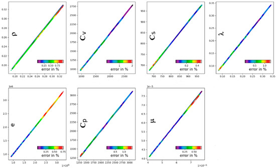
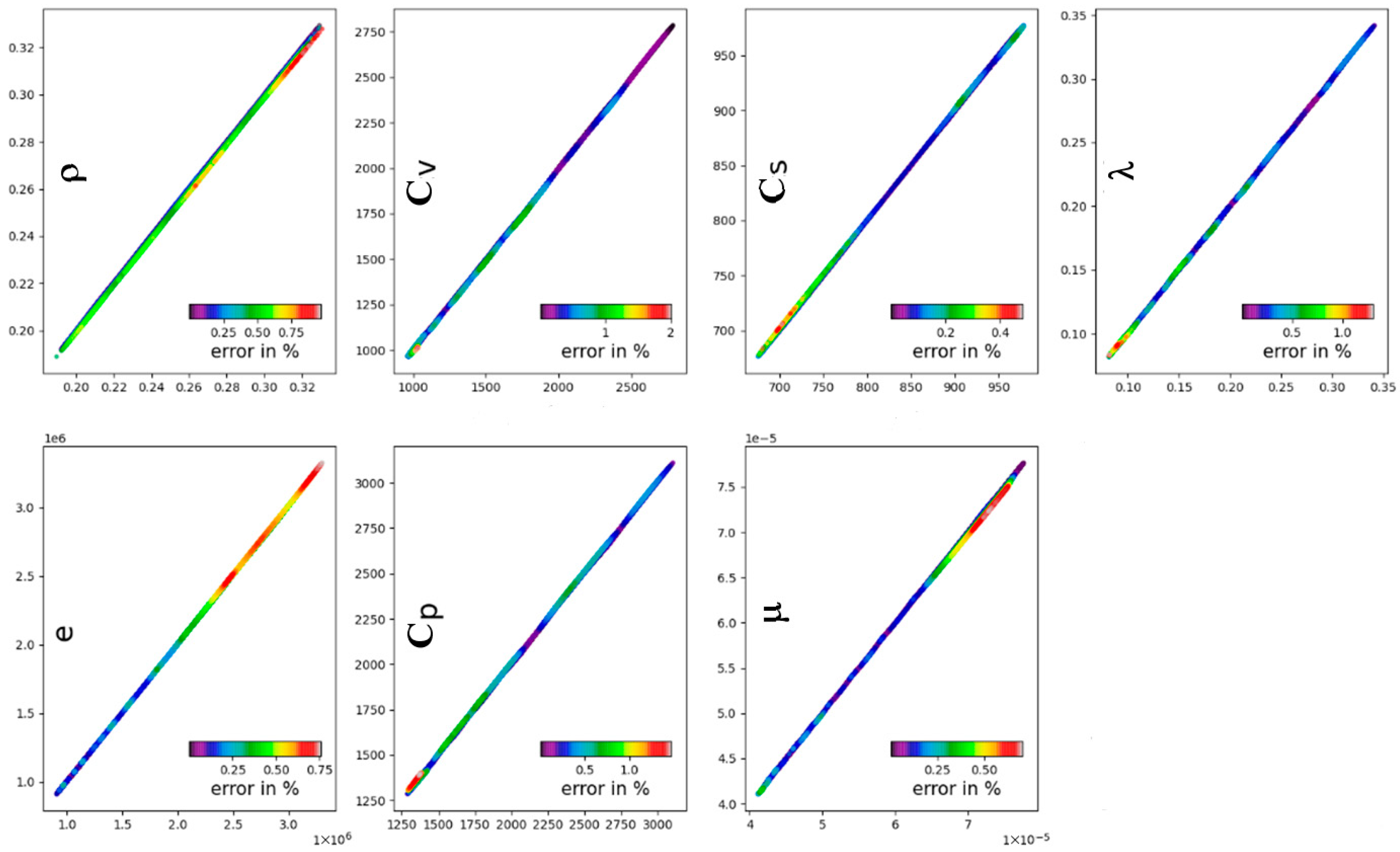
To prepare these simulations, we therefore trained the three neural networks described above (Figure 3 and Table 2). To validate the approach, we tested the neural networks on a range of operations relatively close to the optimal solution (with more than 250,000 test values) to compare the ideal results obtained from the above reference simulation using CARNOT and those predicted by the three neural networks. The comparison is illustrated in Figure 7, which shows that the relative error is very small and that this approach is ready for use in the CFD simulation code.
Table 2.
Multi-Neural Network description.
Figure 7.
CARNOT versus ANN prediction results, colored by relative error.
Using the OPTUNA tool, the neural network architecture and size are defined, as shown in Table 2.
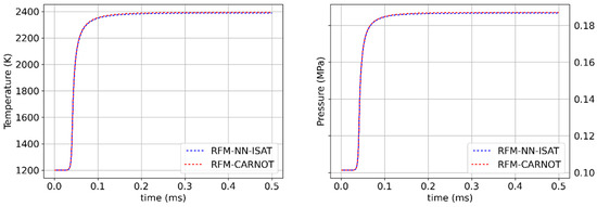
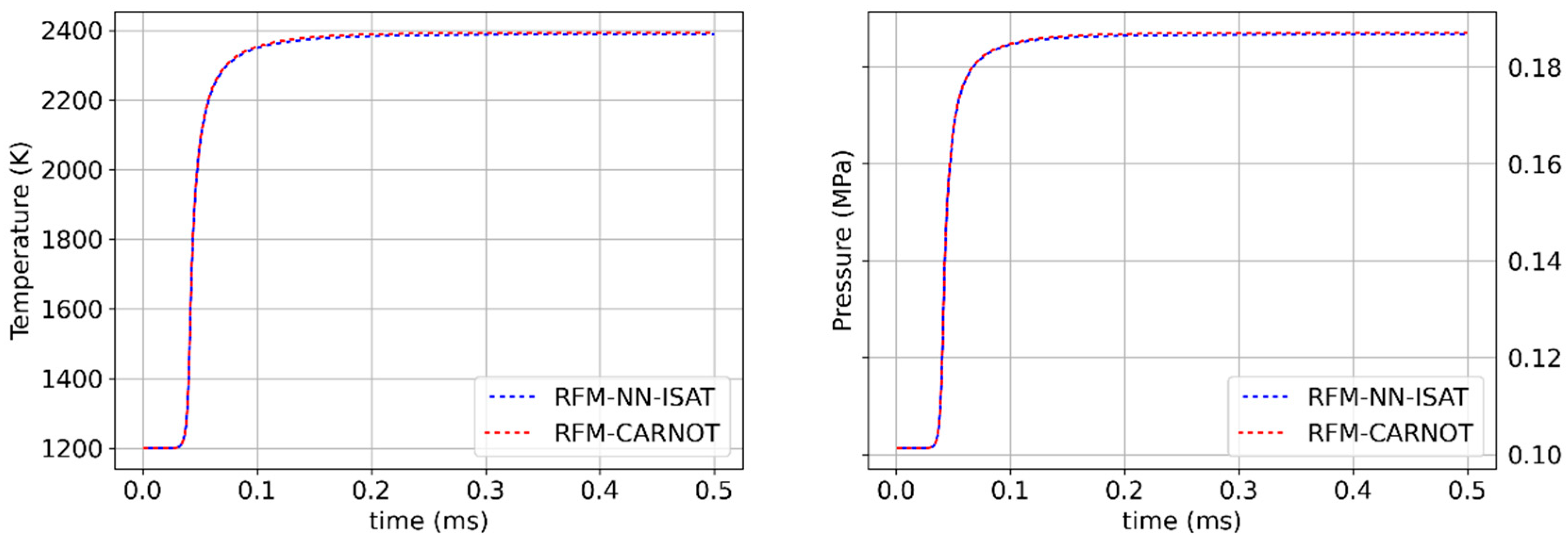
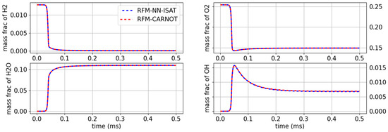
By conducting these methodology comparisons, we aim to assess the accuracy and computational efficiency of the neural network method relative to both a high-fidelity chemistry solver and a direct physics-based approach. Figure 8 and Figure 9 illustrate the pressure, temperature and species mass fractions histories obtained using both methods. As observed in these figures, the RFM-NN-ISAT approach successfully models combustion in the RFM framework. Table 3 presents the execution times, highlighting a significant reduction (20 time less) in computational time when using the RFM-NN-ISAT approach compared to the RFM-CARNOT reference case where RFM is coupled directly to CARNOT using a VLE algorithm for the property’s evaluation. This demonstrates the efficiency gains achieved through the RFM-NN-ISAT neural network-based approach.
Figure 8.
(Left) Temperature and (Right) pressure evolution, with the RFM-NN-ISAT and with the RFM-CARNOT.
Figure 9.
Mass fraction evolution for H2/O2/H2O and OH, with the RFM-NN-ISAT and with the RFM-CARNOT.
Table 3.
Simulation runtime comparison.
Looking ahead, future implementations will leverage GPU-based inference to further accelerate ANN computations, drastically reducing the CONVERGE solver time run and enhancing overall performance.
7. Conclusions
In this paper, we presented an innovative multi-species real fluid modeling methodology using a multi-neural network approach for the simulation of fully compressible two-phase flows with combustion. The integration of the proposed ANN methodology into the CONVERGE CFD solver has significantly improved the accuracy and efficiency of the H2/O2 combustion simulations while drastically reducing computational costs (20 times less) compared to a VLE algorithm for the property’s evaluation using the CARNOT library. The use of ISAT for optimized database generation played a key role in enhancing the performance of the RFM-ANN model by targeting high-gradient thermodynamic regions while minimizing redundant data. Furthermore, multi-neural network approach has revealed an increased robustness and stability of the simulations, highlighting the importance of accurately predicting the density and internal energy in a density-based solver. The results obtained from the combustion of H2/O2 demonstrate that our approach effectively captures changes in thermodynamic properties and species mass fractions during combustion, whilst offering an efficient alternative which, in our view, performs even better than conventional tabulation methods, particularly for simulations involving numerous components. These advancements pave the way for more complex studies considering realistic two-phase combustion configurations. Ultimately, this methodology could be extended to other applications in combustion and fluid dynamics, enabling faster and more accurate modeling of thermodynamic phenomena in complex multi-species environments.
Author Contributions
Conceptualization, B.D. and J.B.; Methodology, B.D. and O.C.; Software, B.D.; Validation, C.H.; Formal analysis, C.H. and O.C.; Investigation, C.H.; Data curation, B.D. and O.C.; Writing—original draft, B.D.; Writing—review & editing, B.D., O.C. and J.B.; Supervision, C.H. and J.B.; Project administration, J.B.; Funding acquisition, J.B. All authors have read and agreed to the published version of the manuscript.
Funding
This research received no external funding.
Institutional Review Board Statement
Not applicable.
Informed Consent Statement
Not applicable.
Data Availability Statement
The original contributions presented in this study are included in the article. Further inquiries can be directed to the corresponding author.
Conflicts of Interest
The authors declare no conflict of interest.
Nomenclature
The following abbreviations are used in this manuscript:
| Symbol | Description | SI Unit |
| ANN | Artificial Neural Network | - |
| CARNOT(X) | Thermodynamic VLE solver | - |
| CFD | Computational fluid dynamics | - |
| CPU | Computer processing unit | s |
| GH2 | Gaseous hydrogen | - |
| ISAT | In Situ Adaptive Tabulation | - |
| LOX | Liquid oxygen | - |
| RFM | Real Fluid Modeling framework | - |
| VLE | Vapor–Liquid Equilibrium | - |
| X | ANN input vector (P, T, Yk) | - |
| Xmin | Lower limit input vector (Pmin, Tmin, Ykmin) | - |
| Xmax | Upper limit input vector (Pmax, Tmax, Ykmax) | - |
| Z | ANN output vector (ρ, e, Cv, Cp, Cs, λ, μ) | - |
| Cp | Specific heat capacity at constant pressure | J·kg−1·K−1 |
| Cv | Specific heat capacity at constant volume | J·kg−1·K−1 |
| Cs | Speed of sound | m·s−1 |
| e | Specific internal energy | J·kg−1 |
| hk | Specific enthalpy of species k | J·kg−1 |
| p, P | Pressure | Pa |
| T | Temperature | K |
| u | Velocity vector | m·s−1 |
| Yk | Mass fraction of species k | - |
| λ | Thermal conductivity | W·m−1·K−1 |
| μ | Dynamic viscosity | Pa·s |
| τ | Viscous stress tensor | Pa |
| ρ | Mixture density | kg·m−3 |
References
- Yang, S.; Yi, P.; Habchi, C. Real-fluid injection modeling and LES simulation of the ECN Spray A injector using a fully compressible two-phase flow approach. Int. J. Multiph. Flow 2020, 122, 103145. [Google Scholar] [CrossRef] [Scilit]
- Yi, P.; Yang, S.; Habchi, C.; Lugo, R. A multicomponent real-fluid fully compressible four-equation model for two-phase flow with phase change. Phys. Fluids 2019, 31, 026102. [Google Scholar] [CrossRef] [Scilit]
- Jafari, S.; Gaballa, H.; Habchi, C.; De Hemptinne, J.-C.; Mougin, P. Exploring the Interaction between Phase Separation and Turbulent Fluid Dynamics in Multi-Species Supercritical Jets using a Tabulated Real-Fluid Model. J. Supercrit. Fluids 2022, 184, 105557. [Google Scholar] [CrossRef] [Scilit]
- Jafari, S.; Gaballa, H.; Habchi, C.; de Hemptinne, J.-C. Towards Understanding the Structure of Subcritical and Transcritical Liquid-Gas Interfaces Using a Tabulated Real Fluid Modeling Approach. Energies 2021, 14, 5621. [Google Scholar] [CrossRef] [Scilit]
- Gaballa, H.; Habchi, C.; de Hemptinne, J.-C. Modeling and LES of high-pressure liquid injection under evaporating and non-evaporating conditions by a real fluid model and surface density approach. Int. J. Multiph. Flow 2023, 160, 104372. [Google Scholar] [CrossRef] [Scilit]
- Delhom, B.; Faney, T.; Mcginn, P.; Habchi, C.; Bohbot, J. Development of a multi-species real fluid modelling approach using a machine learning method. In Proceedings of the ILASS Europe 2023, 32nd European Conference on Liquid Atomization & Spray Systems, Napoli, Italy, 4–7 September 2023. [Google Scholar]
- Srinivasan, N.; Yang, S. Neural Network Aided Adaptive Tabulation with Dynamic Load Balancing for Vapor-Liquid Equilibrium Modeling of Transcritical Multiphase Flows. In Proceedings of the AIAA SCITECH 2026 Forum, Orlando, FL, USA, 12–16 January 2026. [Google Scholar]
- Sahranavardfard, N.; Aubagnac-Karkar, D.; Costante, G.; Rahantamialisoa, F.N.; Habchi, C.; Battistoni, M. Computation of Real-Fluid Thermophysical Properties Using a Neural Network Approach Implemented in OpenFOAM. Fluids 2024, 9, 56. [Google Scholar] [CrossRef] [Scilit]
- Delhom, B.; Habchi, C.; Colin, O.; Bohbot, J. Development of a multi-species real fluid modelling approach using a machine learning method, application to combustion. In Proceedings of the 1st International Symposium on AI and Fluid Mechanics, Chania, Greece, 27–30 May 2025; Paper No [S.16-P.4]. [Google Scholar]
- Pope, S.B. Computationally efficient implementation of combustion chemistry using in situ adaptive tabulation. Combust. Theory Model. 1997, 1, 41–63. [Google Scholar] [CrossRef] [Scilit]
- Ruiz, A.M.; Lacaze, G.; Oefelein, J.C.; Mari, R.; Cuenot, B.; Selle, L.; Poinsot, T. Numerical benchmark for high-Reynolds-number supercritical flows with large density gradients. AIAA J. 2015, 54, 1445–1460. [Google Scholar] [CrossRef] [Scilit]
- Chung, T.H.; Ajlan, M.; Lee, L.L.; Starling, K. Generalized multiparameter correlation for nonpolar and polar fluid transport properties. Ind. Eng. Chem. Res. 1988, 27, 671–679. [Google Scholar] [CrossRef] [Scilit]
- Richards, K.J.; Senecal, P.K.; Pomraning, E. CONVERGE, version 4.1; Convergent Science: Madison, WI, USA, 2025.
- de Hemptinne, J.-C.; Ferrando, N.; Hajiw-Riberaud, M.; Lachet, V.; Maghsoodloo, S.; Mougin, P.; Ngo, T.D.; Pigeon, L.; Yanes, J.R.; Wender, R. CARNOT: A thermodynamic library for energy industries. Sci. Technol. Energy Transit. 2023, 78, 30. [Google Scholar] [CrossRef] [Scilit]
- Akiba, T.; Sano, S.; Yanase, T.; Ohta, T.; Koyama, M. Optuna: A Next-Generation Hyperparameter Optimization Framework. In Proceedings of the 25th ACM SIGKDD International Conference on Knowledge Discovery & Data Mining, Anchorage, Alaska, 4–8 August 2019; pp. 2623–2631. [Google Scholar]
- Aubagnac-Karkar, D.; Mehl, C. NNICE, v1.0. 2023. Available online: https://github.com/aubagnacd/NNICE (accessed on 3 February 2026).
- Burke, M.P.; Chaos, M.; Ju, Y.; Dryer, F.L.; Klippenstein, S.J. Comprehensive H2/O2 kinetic model for high-pressure combustion. Int. J. Chem. Kinet. 2012, 44, 444–474. [Google Scholar] [CrossRef] [Scilit]

Disclaimer/Publisher’s Note: The statements, opinions and data contained in all publications are solely those of the individual author(s) and contributor(s) and not of MDPI and/or the editor(s). MDPI and/or the editor(s) disclaim responsibility for any injury to people or property resulting from any ideas, methods, instructions or products referred to in the content. |
© 2026 by the authors. Licensee MDPI, Basel, Switzerland. This article is an open access article distributed under the terms and conditions of the Creative Commons Attribution (CC BY) license.