Experimentally Validated Discrete Phase Model for PM_2.5 and PM₁₀ with Numerical Transport Mapping

Abstract

Indoor exposure to particulate matter (PM) depends on ventilation-driven transport, yet sensor placement in real rooms is often based on limited point data. This study develops and experimentally validates a transient CFD framework, using RANS airflow coupled with Lagrangian discrete phase tracking, to map PM_2.5 and PM₁₀ in a full-scale 2.0 × 3.0 × 2.5 m bedroom with a fixed, non-oscillating pedestal fan and an open window. Airflow was verified by grid independence and validated against 10-point velocity measurements (RMSE = 0.108 m·s⁻¹). Incense experiments (≈31 min burn) provided PM time series over the first 60 min at 16 locations on two heights; emission rate, burning time, and air-change rate (1.96–5.39 ACH) were calibrated so that accepted models achieved aggregate R² > 0.90. Spatial mapping on a 0.5 m grid shows that PM behavior is governed primarily by airflow-defined accumulation pockets rather than by source proximity alone. A near-source region consistently captured strong early-time peaks, whereas remote low-exchange pockets remained elevated during the decay phase. For PM_2.5, the most persistent hotspot is a ceiling-adjacent recirculation pocket, while for PM₁₀, gravitational settling shifted the dominant hotspots toward floor-layer, low-velocity regions. An exposure score combining normalized peak and time-averaged concentrations, interpreted together with particle-track persistence metrics, distinguished transiently traversed regions from true retention pockets. The results show that sensor placement should follow the monitoring objective: near-source regions are more responsive to peak events, ceiling pockets are more suitable for persistent PM_2.5 monitoring, and floor hotspots are more critical for PM₁₀. No single fixed sensor location adequately represents both particle sizes in the present bedroom and ventilation configuration.

1. Introduction

Human exposure to air pollutants is largely determined indoors, where many sources are present and ventilation and airflow organization control dilution and transport. Indoor combustion and consumer activities can create short, high-magnitude concentration events (including those linked to incense products), while ventilation can both dilute and redistribute contaminants depending on boundary conditions and flow paths [1,2,3,4]. CO₂ remains a practical operational indicator for ventilation adequacy, but its interpretation depends on where and how it is measured, and natural ventilation feasibility can be constrained by outdoor air quality conditions [5,6]. Field monitoring combined with modeling also shows that “smart” ventilation strategies can shift indoor air quality (IAQ) metrics while exposing limitations when indoor sources are not well-characterized [7].

A central technical issue is that indoor pollutant fields are often non-uniform. They are typically driven by stratification, jets, recirculation, and room geometry, so a single “representative” height or location is hard to justify. Validated studies report meaningful vertical gradients in classroom CO₂ and height-dependent exposure differences across pollutants (e.g., ozone versus PM_2.5), and similar height-plane effects appear in field-plus-computational-fluid-dynamics (CFD) kitchen studies [8,9,10]. CFD coupled with office measurements also shows that vent configuration can redistribute CO₂ and particle fields and create dead or stagnant regions [11]. More advanced room-scale modeling further indicates that ventilation strategy can alter exposure pathways and that sparse sampling can miss local peaks [12].

Because pollutant fields are spatially non-uniform, a fixed sensor’s reading depends strongly on where it is installed. Placement therefore determines what the measurement represents. Exposure studies show that breathing-zone concentrations can exceed readings from fixed monitors, and that the best stationary location depends on the pollutant and occupant state (e.g., sitting vs. standing; static vs. moving), with PM often easier to infer than CO₂ [13,14]. Across many indoor activities (including incense), exhaust-duct and ceiling-center PM signals can track peak events similarly, though agreement can weaken during decay [15]. Office incense tests likewise show that the location that best tracks the breathing-zone mean can change with the ventilation configuration [16]. Air-cleaning and airflow interventions reinforce the same point: Airflow interactions can create dead zones and uneven zone performance that averages can hide [17]. Related IAQ studies also use hybrid CFD–multizone modeling in mechanically ventilated confined spaces and show that heating, ventilation, and air conditioning (HVAC) intake/inlet design can change PM ingestion and energy demand [18,19]. Together, these studies show that PM distributions, and the effectiveness of control measures, are driven by ventilation configuration and airflow structure.

In practice, deployments often rely on only one or a few sensors, so the location must match the monitoring objective. When sensor count is constrained, placement becomes a trade-off between capturing episodic peaks and representing longer-term exposure. Long-term office datasets show sparse sensors can capture trends, but peak-event detection needs denser placement and much shorter sampling, with HVAC type and room size strongly affecting CO₂ event risk [20]. Optimization studies further show that “optimal” layouts depend on season, ventilation mode, and occupancy, while experimental evaluations highlight conflicts when multiple IAQ metrics share a sensor package [21,22,23]. Prior studies also show that indoor pollutant fields can vary with height and ventilation configuration [8,24], that the representativeness of a fixed sensor depends on how well it reflects breathing-zone exposure and can vary with pollutant and occupant activity [14], that monitoring design must distinguish between temporal trend tracking and high-concentration event detection [20], and that single-point CO₂ measurements can introduce uncertainty when used to infer far-field exposure under spatially varying ventilation flows [25].

However, these studies stop short of providing a direct workflow for converting validated transient PM transport in a specific room into explicit sensor-placement guidance. In practice, the most suitable location can differ depending on whether the priority is sustained concentration, short-duration peaks, or overall representativeness of room conditions. This study addresses that need by applying an experimentally validated transient CFD framework to PM_2.5 and PM₁₀ transport in a full-scale bedroom and by converting the resulting spatial–temporal fields into an objective-based sensor-placement assessment of candidate monitoring regions. These regions are then evaluated using an exposure score that combines peak and time-averaged concentration, while particle-track persistence metrics are used to interpret whether highly ranked regions reflect broad particle reach or prolonged local retention. Through this approach, the study provides a physics-based basis for identifying monitoring locations that are more suitable for persistent exposure assessment and those that are more responsive to strong local PM events. Section 2 describes the experimental setup, numerical model, calibration procedure, and post-processing framework for spatial mapping and exposure metrics. Section 3 presents the validated PM_2.5 and PM₁₀ distributions, discusses the resulting exposure score maps, and examines their implications for sensor placement in the bedroom. Section 4 summarizes the main findings and outlines how the approach can be extended to other room geometries and ventilation strategies.

2. Materials and Methods

2.1. Case-Study Room and Numerical Model

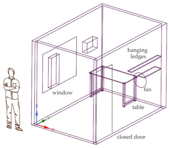
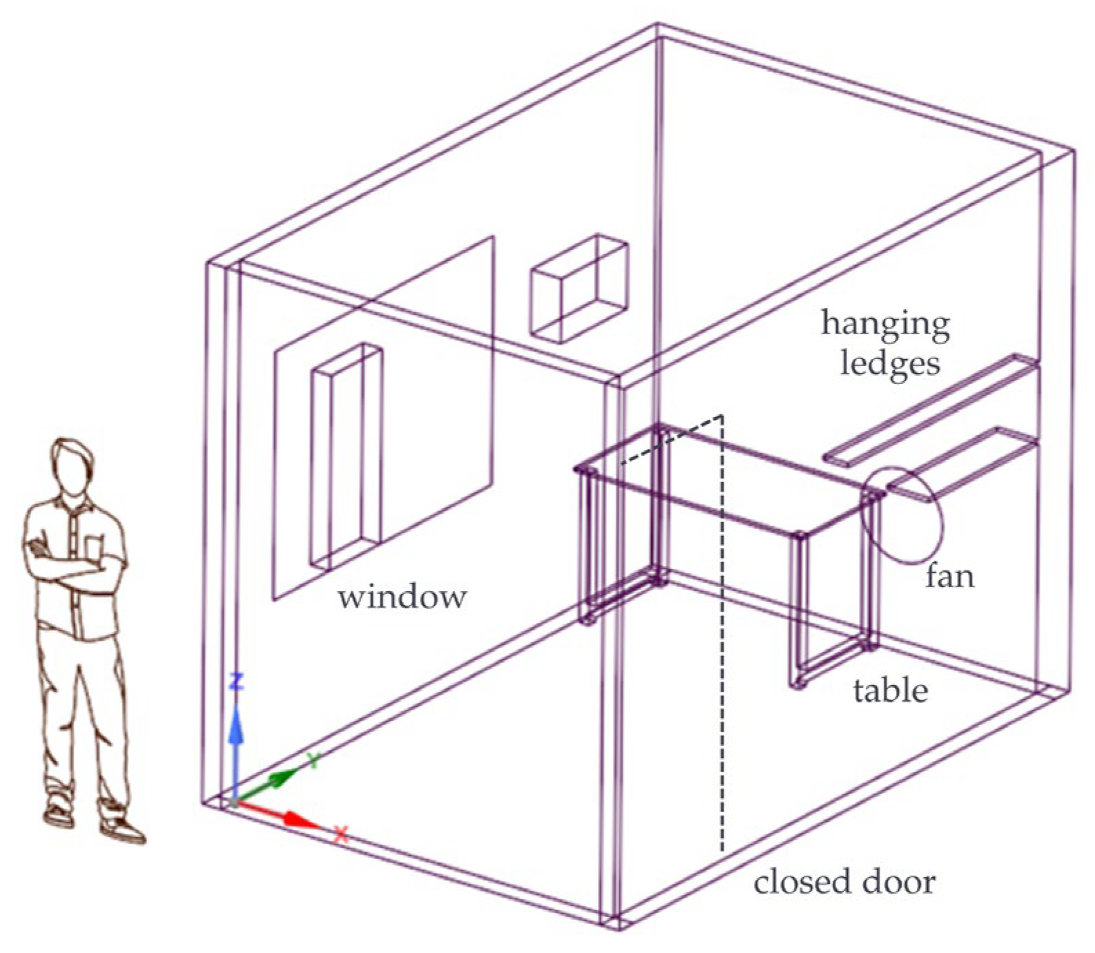
The PM case study is conducted in an unused bedroom converted into a stockroom. The room has internal dimensions of 2.0 m (length) by 3.0 m (width) by 2.5 m (height). It contains only a table and a fixed, non-oscillating pedestal fan, which serves as the sole mechanical ventilation device. The bedroom includes an operable window on one wall and a door with a gap at the bottom of the opposite wall. The window provides air exchange with the outdoor environment and introduces a natural ventilation component that interacts with the fan-induced flow. The combination of fan-driven circulation and window-driven exchange allows assessment of how external air supply influences the dispersion and removal of PM_2.5 and PM₁₀ in a small residential room. Figure 1 shows the three-dimensional geometry of the bedroom.

Figure 1. 3D geometry of the bedroom, including the fan and other fixtures. The dashed line indicates the closed door.

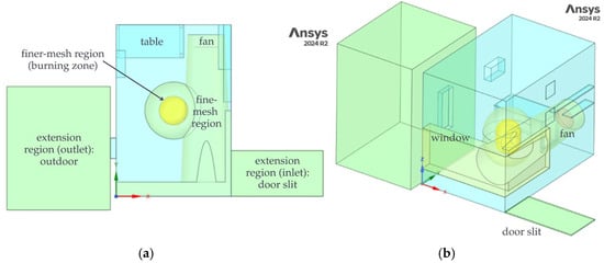
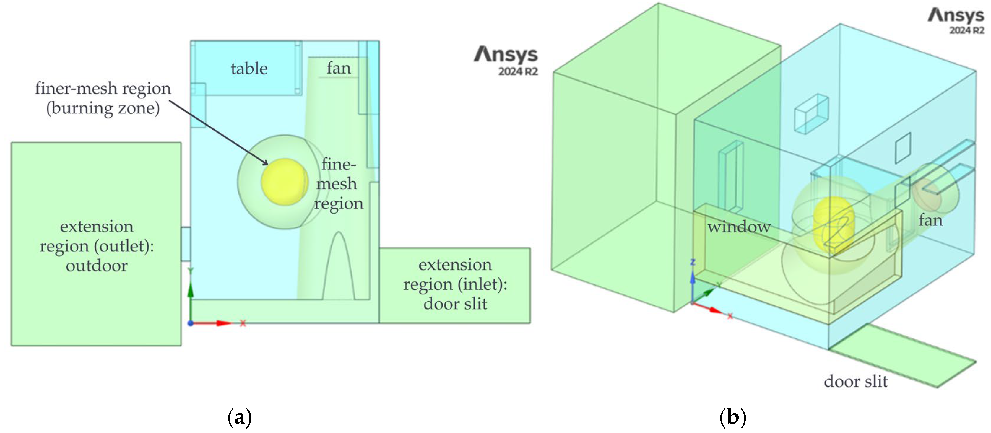
The computational domain, displayed in Figure 2, reproduces this indoor environment while retaining features that significantly affect airflow and particle transport. The main room volume represents the physical enclosure, including walls, floor, and ceiling. The table and pedestal fan are modeled explicitly as flow obstructions, whereas smaller objects are omitted to reduce mesh size. To control mesh refinement near key flow and pollutant sources, the room is partitioned into multiple subdomains. The main room volume acts as a coarse region. A nested subdomain surrounding the fan and incense source defines a fine-mesh region, and a smaller inner subdomain encloses the burning zone of the incense stick, where the highest particle gradients are expected. Additional flow-extension volumes are attached to the door gap and window opening. These extensions allow the flow to develop before entering or leaving the main room and reduce numerical artifacts at the physical openings. Shared topology is imposed across all subdomains so that interfaces between the main, fine, and extension regions are conformal. The geometry is created using Ansys SpaceClaim 2024 R2 (Ansys Inc., Canonsburg, PA, USA).

Figure 2. Computational domain: (a) top view, (b) isometric view.

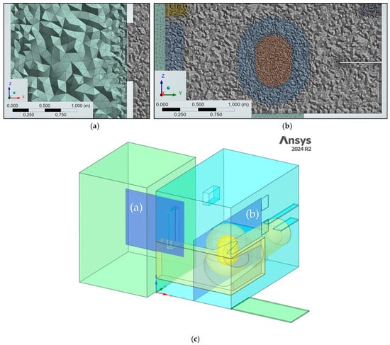
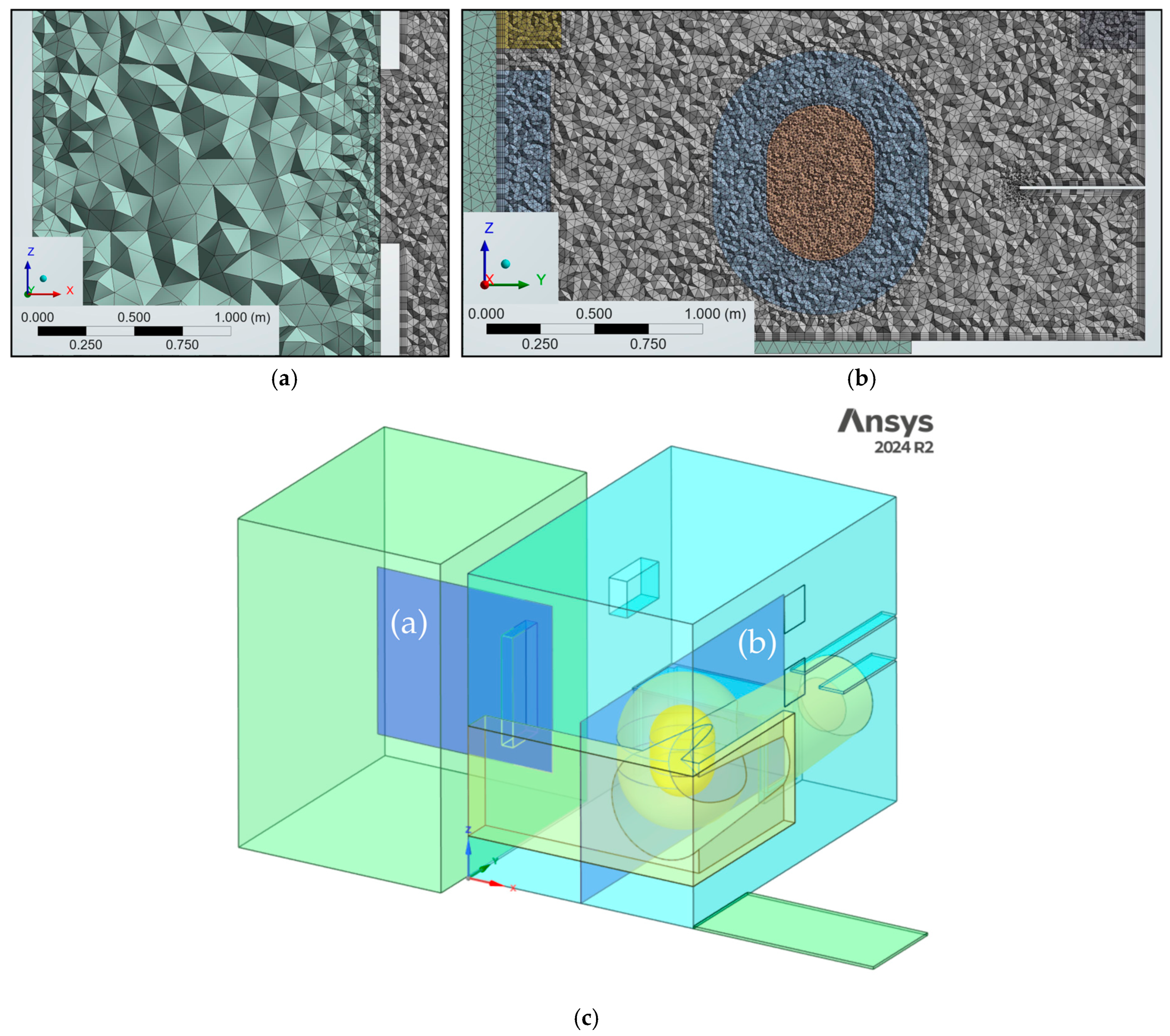
Meshing is performed in Ansys Meshing 2024 R2 (Ansys Inc., Canonsburg, PA, USA) using a hybrid unstructured grid. The base room region uses a uniform body size of 75 mm, while the fine and finer subdomains surrounding the fan and incense use body sizes of 25 mm and 15 mm, respectively. The fan surface is meshed with a target face size of 10 mm, and the door gap extension uses body sizes of 4 mm to resolve the narrow opening. Inflation layers are generated on all solid walls with an initial thickness of 5 mm to resolve near-wall velocity and turbulence gradients, which is needed to capture recirculation and deposition-relevant flow features. The resulting mesh, in Figure 3, contains approximately 4.5 million cells. A grid-independence study for the airflow solution is described in Section 2.3; further refinement beyond this mesh produces negligible changes in the validation quantities, so it is adopted for all subsequent simulations.

Figure 3. Mesh slices: (a) XZ plane at the center of the window opening, (b) YZ plane at the center of the finer-mesh region, and (c) location of the slices shown in (a) and (b) within the computational domain.

Airflow in the bedroom is modeled as an incompressible, Newtonian fluid governed by the Reynolds-averaged Navier–Stokes equations and the continuity equation. A pressure-based solver is used, appropriate for the low-Mach indoor-flow conditions considered. Turbulence is represented using the realizable k−ε model, selected because of its demonstrated performance in indoor airflow applications with recirculation, separation, and buoyancy-influenced mixing. The model provides improved handling of strain and rotation compared with the standard k−ε formulation while remaining computationally efficient. Spatial discretization for momentum and turbulence equations employ second-order upwind schemes, and gradients are evaluated using a least-squares method. Pressure–velocity coupling is achieved with a pressure-based segregated algorithm, and all residuals are reduced below 10⁻⁵ before a time step is accepted as converged. These settings are applied consistently to both the airflow-only and particle-laden simulations. All CFD simulations are performed using the finite-volume solver ANSYS Fluent 2024 R2 (Ansys Inc., Canonsburg, PA, USA).

The boundary conditions for the airflow simulation are summarized in Table 1. Air enters the bedroom through the door gap, modeled as a mass-flow inlet, and exits through the window-side extension, defined as an outflow boundary so that the total discharge is determined by the inlet and internal pressure field. In the CFD model, this door gap is the only explicit mass-flow inlet and the window-side extension is the outlet, providing a simple, well-defined inlet–outlet pair that idealizes the experimental configuration and does not imply that all real inflow occurs exclusively through the gap. The pedestal fan is represented by a fan boundary condition that imposes a prescribed pressure jump across the fan disk, aligned with the fan axis. In the external extension domain beyond the window, vertical faces are treated as symmetry planes and horizontal faces as slip walls, approximating an unobstructed outdoor environment. All faces corresponding to the room envelope and furniture surfaces are modeled as no-slip walls.

Table 1. Boundary conditions for airflow-only simulation.

Boundary	Face/s	Type	Settings	Value
inlet	door gap	mass-flow inlet	mass-flow rate [kg/s]	0.0196
			turbulence intensity [%]	3
			hydraulic diameter [m]	0.039
outlet	parallel to window face	outflow	flow rate weighting	1
fan	fan	fan	pressure jump (constant) [Pa]	2.5
			fan axis	(0, −1, 0)
			fan origin	(1.58, 2.61, 0.84)
			fan hub radius [m]	0.055
			tangential/radial velocity profile [m/s]	0
symmetry	perpendicular vertical faces at the window extension	symmetry
wall	perpendicular horizontal faces at the window extension	wall	shear condition	slip
	room, furniture		shear condition	no-slip

The airflow is solved using a transient RANS formulation. A second-order implicit time discretization is used to improve temporal accuracy in capturing the fan-driven jet and its interaction with the window opening. The simulation is advanced for 800 time steps with a step size Δt = 3 s and a maximum of 20 inner iterations per time step. This duration is sufficient for the velocity readings at all probe locations to stabilize, and time averaging for validation is performed over this quasi-steady period.

Particulate pollutant transport (PM_2.5 and PM₁₀) is modeled using a Lagrangian discrete phase model (DPM), which tracks particle trajectories within the continuous air phase. Particle trajectories are advanced with a particle time step of 0.05 s using high-resolution tracking, a step length factor of 5, and a maximum of 10⁸ tracking steps to avoid premature termination of long-lived trajectories. Spherical anthracite particles are used as an inert surrogate for both PM_2.5 and PM₁₀, with a material density of 1550 kg·m⁻³. Evaporation, break-up, and chemical reactions are neglected. Gravitational acceleration is enabled (g = 9.81 m·s⁻² in the −z direction) so particle motion includes gravitational settling in addition to drag and turbulent dispersion. The DPM includes the Saffman lift to capture shear-induced lateral forces in regions with strong velocity gradients, a stochastic collision model to account for inter-particle collisions in locally dense regions, and inelastic wall collisions modeled with constant coefficients of restitution 0.9 in the normal direction and 0.9 in the tangential direction. The restitution-coefficient assumption is consistent with values used in prior particle transport simulations and reported sensitivity checks [26,27,28,29].

Ten sequential injection points are used to represent the progressive downward motion of the burning zone along the incense stick. The injection coordinates and activation intervals are summarized in Table 2. The injections are arranged so that only one is active at any given time, each operating for one tenth of the total burning time, t_b. In this way, the effective source descended as the incense length decreased. Injection velocity is set to 0 m·s⁻¹, representing a stationary source without directed jet momentum. Monodisperse particles are used for each size fraction, with diameters d_p = 2.5 × 10⁻⁶ m for PM_2.5 and d_p = 1.0 × 10⁻⁵ m for PM₁₀. The actual size distribution of incense smoke could not be characterized experimentally; these values therefore represent nominal diameters for each regulatory size class. For each sampling volume defined below, the tracked particle mass within the control volume is converted into a volume-averaged concentration, yielding time-dependent PM_2.5 and PM₁₀ histories directly comparable with the experimental sensor records.

Table 2. Injection location and activation time.

Injection	Coordinates	Start Time, s	Stop Time, s
inj-01	(1, 1.5, 0.84)	0	tb/10
inj-02	(1, 1.5, 0.818)	tb/10	2tb/10
inj-03	(1, 1.5, 0.796)	2tb/10	3tb/10
inj-04	(1, 1.5, 0.774)	3tb/10	4tb/10
inj-05	(1, 1.5, 0.752)	4tb/10	5tb/10
inj-06	(1, 1.5, 0.73)	5tb/10	6tb/10
inj-07	(1, 1.5, 0.708)	6tb/10	7tb/10
inj-08	(1, 1.5, 0.686)	7tb/10	8tb/10
inj-09	(1, 1.5, 0.664)	8tb/10	9tb/10
inj-10	(1, 1.5, 0.642)	9tb/10	tb

Buoyancy is included by solving the energy equation and applying the Boussinesq approximation with a reference density of ρ₀ = 1.177 kg∙m⁻³ at T₀ = 300 K and thermal expansion coefficient β = 1/300 K⁻¹. To represent the buoyant plume generated by the burning tip without explicitly modeling combustion or imposing a point heat source at the tip, a localized volumetric thermal forcing is prescribed in a near-source control volume surrounding the active injection location. Cylindrical volumes of radius r = 0.03 m and height h = 0.06 m are defined around the injection points and are separated to the finer mesh using cell registers. Because adjacent cylinders overlap, the union of these cylinders is partitioned into 19 non-overlapping regions to prevent double counting of heat addition in shared cells. A user-defined function (UDF) applies the volumetric energy source only to the currently active region(s), synchronized with the sequential injection schedule. The forcing is implemented so that the total heat input is conserved by distributing a constant heat rate, Q, over the active region volume V_active(t), in Equation (1).

$$S_E\left(t\right)=Q/V_{\mathrm{active}}\left(t\right)$$

(1)

For the DPM simulations, the airflow geometry is augmented with 0.30 m × 0.30 m × 0.30 m sampling volumes centered at each experimental probe location, shown in Figure 4. These “virtual sensor” boxes are used to compute volume-averaged PM concentrations representative of the sensor locations, because the DPM does not directly provide point concentrations. The underlying airflow mesh is retained, but the additional boxes required local remeshing. Boxes that did not intersect walls are meshed with structured hexahedral elements, whereas those intersecting walls used unstructured tetrahedra to remain compatible with the existing inflation layers. The total cell count increased from 4.5 to 4.8 million cells.

Figure 4. Computational domain with sampling volumes.

2.2. Experimental Measurements

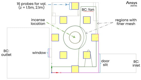
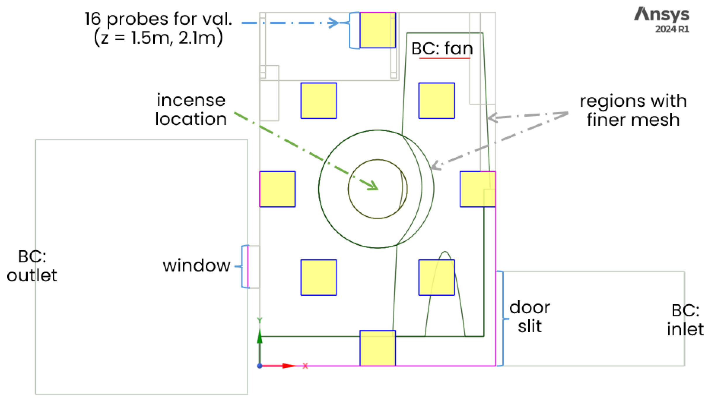
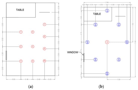
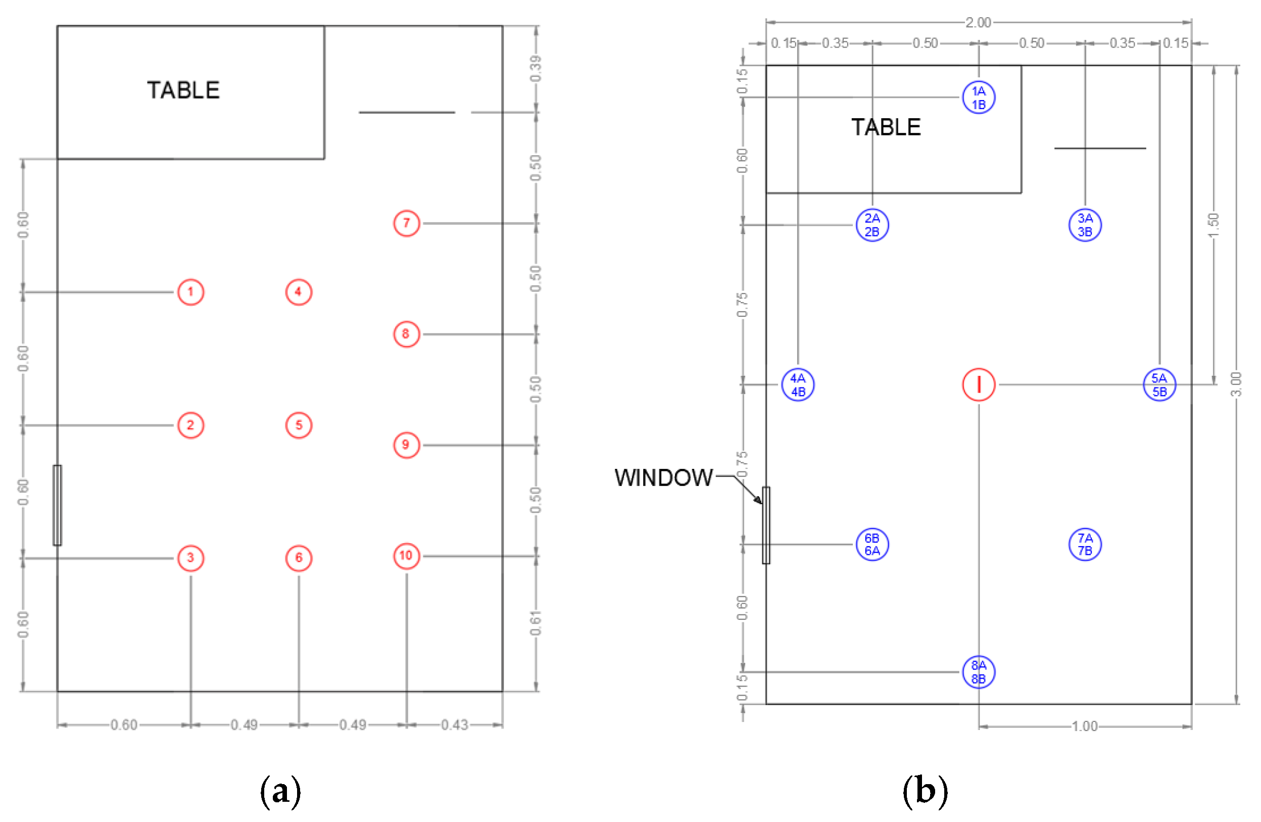
Air velocity measurements are taken to validate the airflow solution. Ten probe locations, corresponding to virtual monitoring points in the CFD model, are positioned at a height of z = 0.84 m, approximately at fan mid-height. The probes form a 3 × 4 grid, as seen in Figure 5a, that captures the main recirculation region in front of the fan and the downstream zone towards the window. This layout ensures that both the core of the fan jet and the surrounding recirculation zones are sampled.

Figure 5. Probing locations for (a) airflow and (b) PM measurements. Numbers indicate the probe IDs.

Particulate matter experiments are performed using two incense sticks as a combined source of PM_2.5 and PM₁₀. To reduce source variability across trials, all runs use incense sticks from the same product pack, the same two-stick configuration, and the same burn-start sequence before measurements begin. The incense sticks are placed at the center of the room, with the burnable tip at z = 0.84 m. A single Aeroqual SH PM optical particle sensor is used to measure PM_2.5 and PM₁₀ concentrations. In Figure 5b, sixteen probe locations are defined at two heights, z = 1.5 and 2.1 m, arranged as two diamonds covering the main occupied region. Because only one sensor is available, multiple experimental runs are conducted; in each run, the sensor is relocated to a new probe location until all 16 positions at both heights have been measured. During each trial, the incense burns for approximately 31 min and the sensor logs concentrations for 120 min; only the first 60 min are used for calibration and validation, capturing the build-up phase and the decay after the source extinguishes.

2.3. Model Calibration, Validation, and Spatiotemporal Mapping

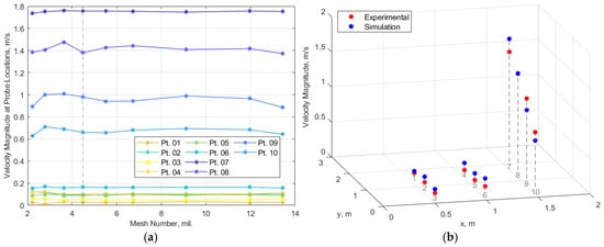
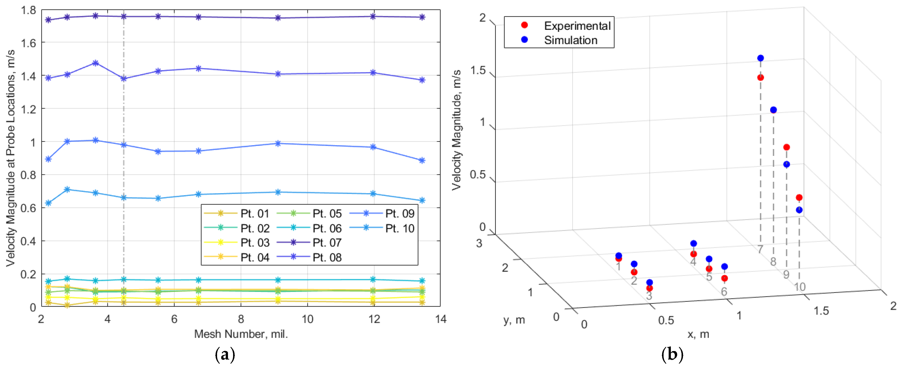
A mesh-independence study is conducted for the bedroom by progressively refining the unstructured grid and monitoring velocity predictions at the probe locations. Shown in Figure 6a, velocity magnitudes at the ten probes are plotted against total cell count. Beyond 4.5 million cells, further refinement produces negligible changes in predicted velocities at all probes. This mesh is therefore selected as the reference grid and is reused in all subsequent airflow–particle simulations. Using the same mesh for both verification and pollutant simulations ensures that the verified spatial resolution directly underpins the PM dispersion results.

Figure 6. Airflow verification and validation through (a) grid-independence study and (b) simulation validation.

Airflow validation is then performed by comparing simulated and measured air velocities at the bedroom probes, displayed in Figure 6b. The comparison is visualized as a 3D plot where red markers denote experimental data, and blue markers denote simulation results at the same locations. Agreement is quantified using the root-mean-square error (RMSE) of velocity magnitude across all probes. For the bedroom, the RMSE is 0.108 m·s⁻¹, which is substantially lower than the characteristic mean velocities in the fan jet. This indicates good consistency between the CFD predictions and measurements. Residual discrepancies are attributed to unsteady fan operation, and simplifications in the computational model, such as the idealized fan boundary condition and the omission of small geometric details. Given the grid-independence check and probe validation, the airflow solution is used as the input field for DPM tracking and PM mapping.

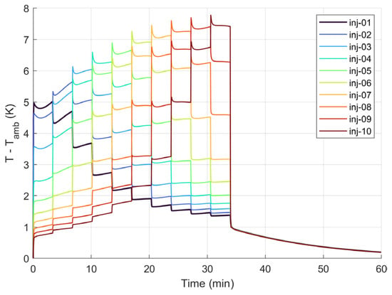
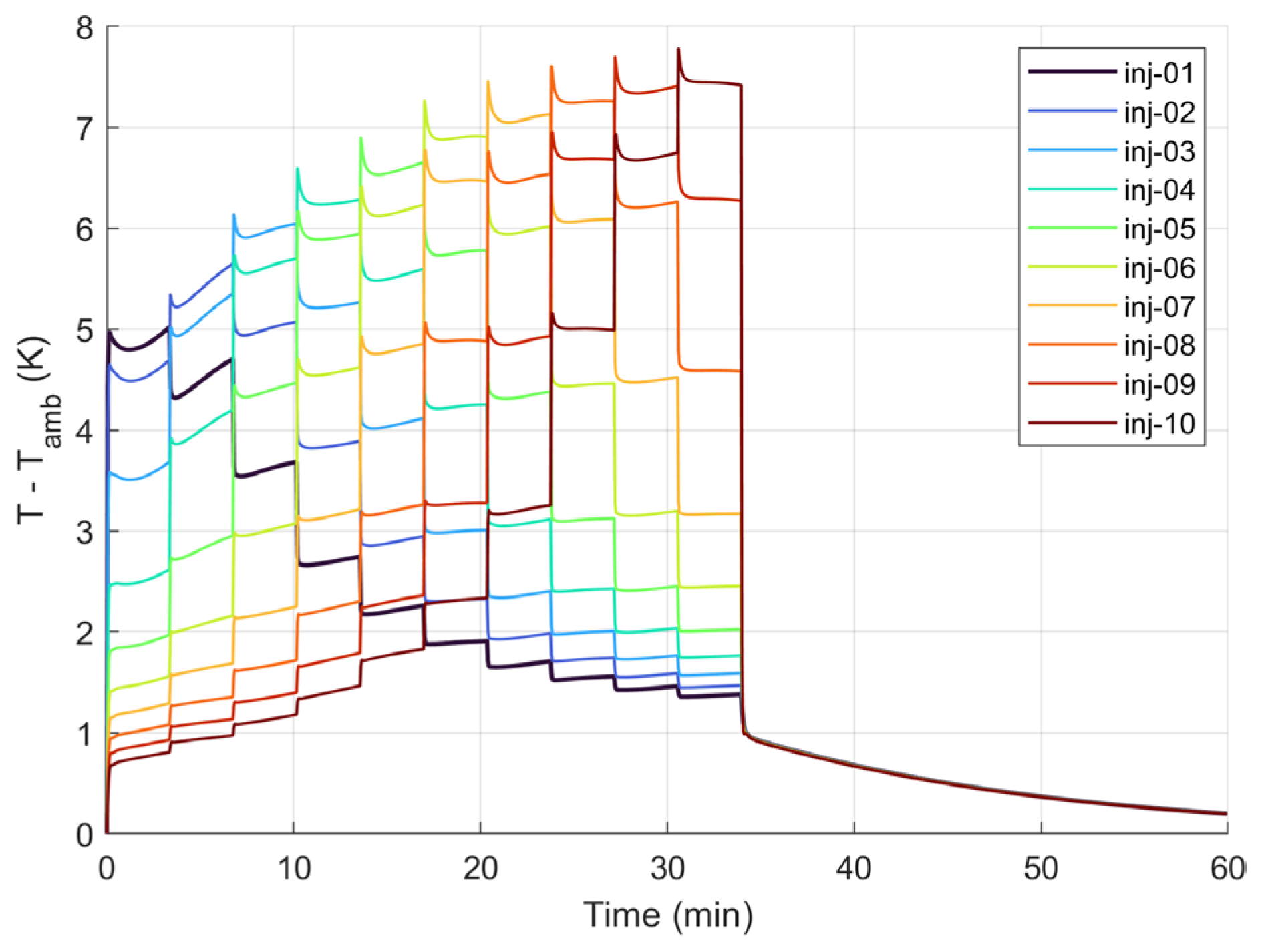
For specifying the magnitude of the near-source thermal forcing in the buoyancy UDF, the heat input Q is estimated from near-source temperature measurements used to bound the plume forcing magnitude. Air temperature was recorded using a Fluke 922 (Fluke Corporation, Everett, WA, USA) temperature probe positioned horizontally toward the burning tip at a radial distance of 0.03 m under room conditions (n = 3 trials; 1 min per trial). In a representative trial, the measured near-source temperature rise relative to ambient was ΔT = 5.92 ± 0.27 K (mean ± SD over 60 samples), with instantaneous values spanning 5.6–7.0 K. Using this bound, the thermal forcing magnitude was set to Q = 20 W and applied as a volumetric source within the active near-source region(s). The resulting near-source (T-T_amb) time histories are shown in Figure 7, which confirms the sequential activation of injection locations and a bounded thermal response within the intended near-source volume.

Figure 7. Injection-region volume-averaged temperature rise.

For the particulate phase, the key unknowns are the incense emission rate, burning time, and room air-change rate. These parameters are calibrated by matching CFD predictions to experimental PM time series. A total of 32 CFD simulations are initially run, grouped into four sets corresponding to PM_2.5 and PM₁₀ at z = 1.5 and 2.1 m. Emission rate, burning time, and inlet mass-flow rate are varied within the ranges listed in Table 3. For example, PM_2.5 at z = 2.1 m uses emission rates between 4.24 and 6.45 µg·s⁻¹, burning times of 31–34 min, and inlet mass-flow rates of 0.0098–0.0245 kg·s⁻¹, while PM₁₀ cases used proportionally higher emission rates. During analysis, it becomes clear that the experimental time series at four probe locations—2A and 3A at z = 2.1 m and 1B and 7B at z = 1.5 m—are unreliable, so the corresponding CFD candidates are discarded from the calibration set. This reduces the usable pool from 32 to 24 CFD models.

Table 3. PM DPM parameters.

Simulation Group	Emission Rate [µg/s]	Burning Time [min]	Inlet Mass-Flow Rate [kg/s]	Equivalent Air-Change Rate [ACH]
PM2.5, z = 2.1m	4.24–6.42	31–34	0.0098–0.0245	1.96–4.90
PM2.5, z = 1.5m	3.62–5.50	31–34	0.0147–0.02695	2.94–5.39
PM10, z = 2.1m	6.51–11.83	31–34	0.0098–0.0245	1.96–4.90
PM10, z = 1.5m	6.83–10.69	31–34	0.0147–0.02695	2.94–5.39

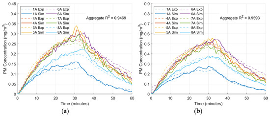
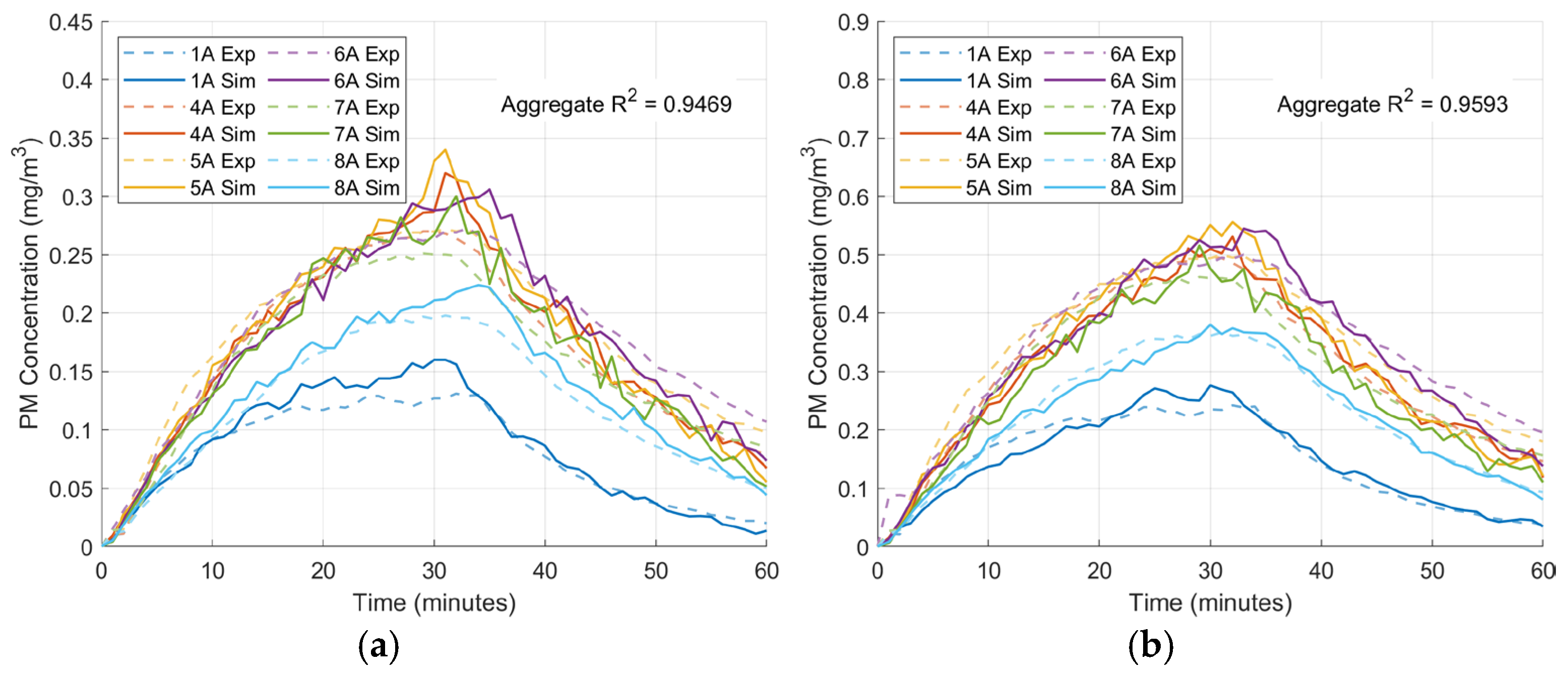
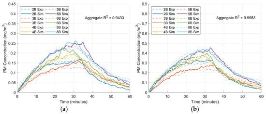
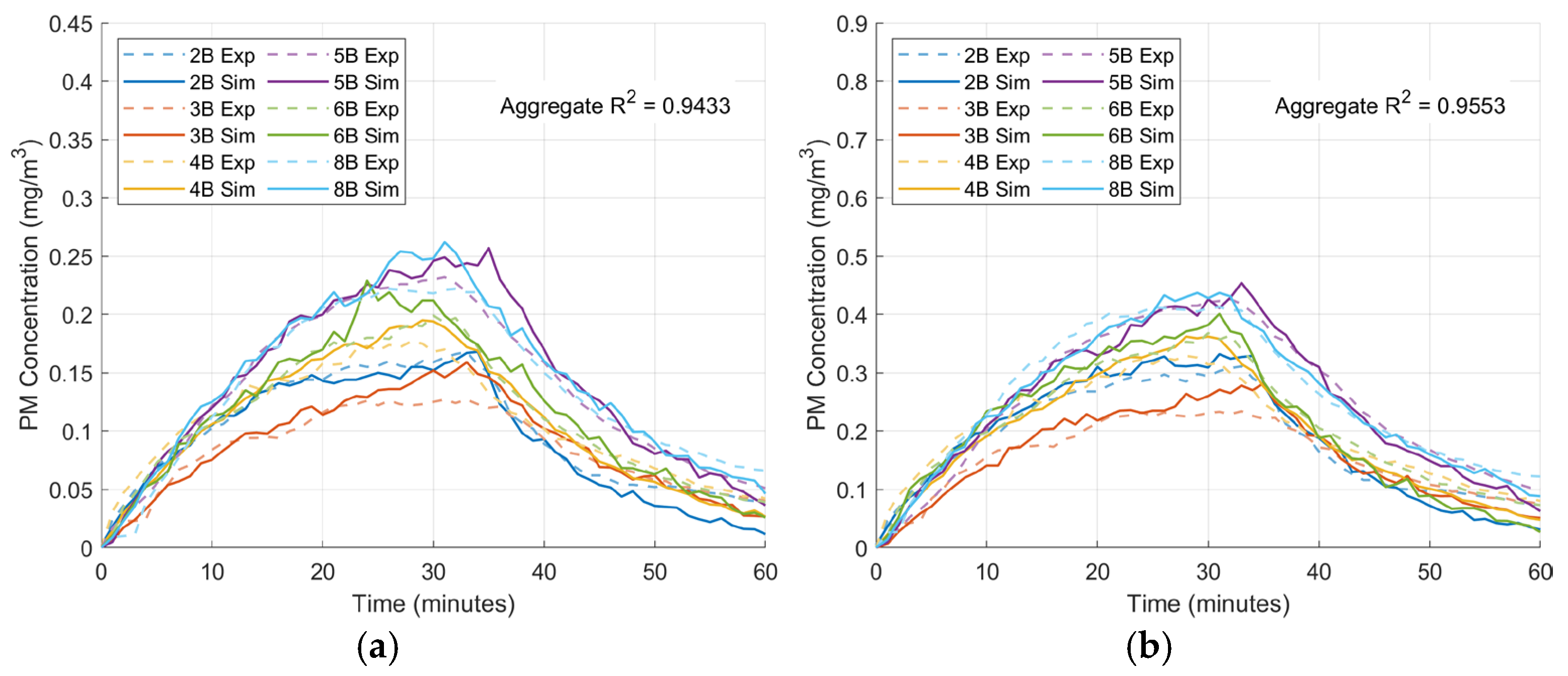
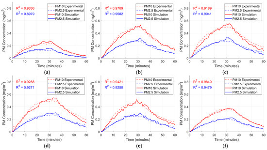
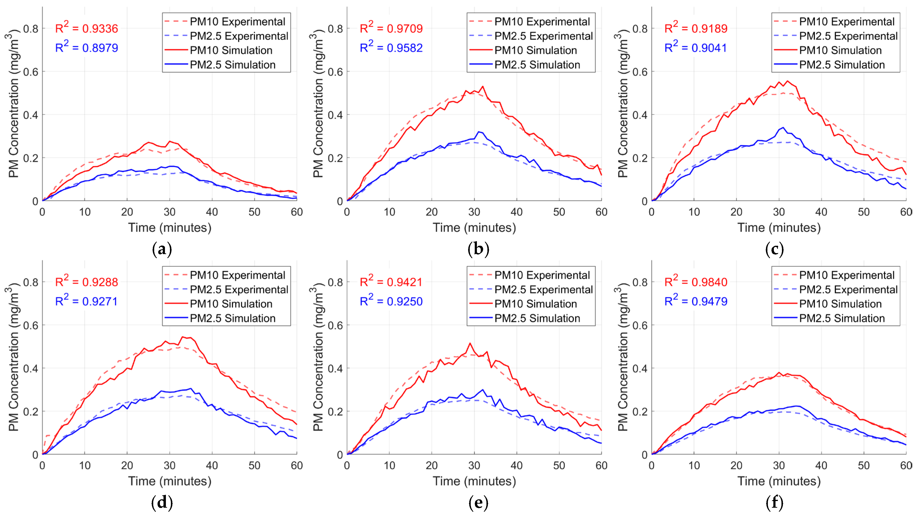
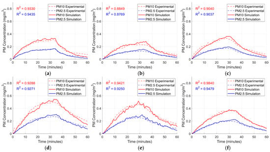
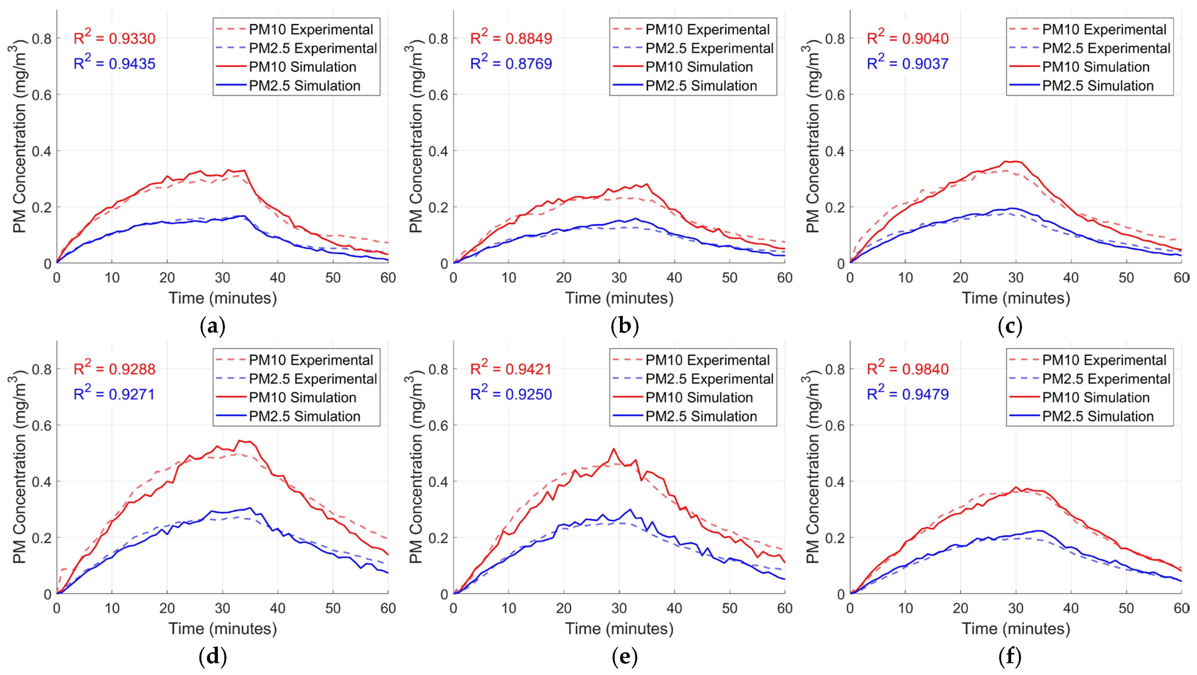
From these 24 runs, models are selected for which PM time series matches the experimental measurements for the remaining probes in each group. For all accepted models, the aggregate coefficient of determination (R²) across the four probes in the group exceeds 0.90, as shown in Figure 8 for probes at z = 2.1 m and Figure 9 for probes at z = 1.5 m. The corresponding segregated validation plots in Figure 10 and Figure 11 show the individual experimental and simulated time series for each probe at z = 2.1 m and z = 1.5 m, respectively. Individual-probe R² values vary, but the group-level aggregate remains consistently above 0.90. These calibrated models form the basis for the subsequent spatial mapping of PM_2.5 and PM₁₀ distributions and the sensor-placement analysis.

Figure 8. PM consolidated simulation validation (z = 2.1 m): (a) PM_2.5, (b) PM₁₀.

Figure 9. PM consolidated simulation validation (z = 1.5 m): (a) PM_2.5, (b) PM₁₀.

Figure 10. PM segregated simulation validation (z = 2.1m): models (a) 1A, (b) 4A, (c) 5A, (d) 6A, (e) 7A, and (f) 8A.

Figure 11. PM segregated simulation validation (z = 1.5m): models (a) 2B, (b) 3B, (c) 4B, (d) 5B, (e) 6B, and (f) 8B.

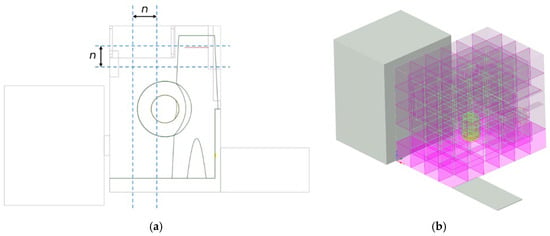
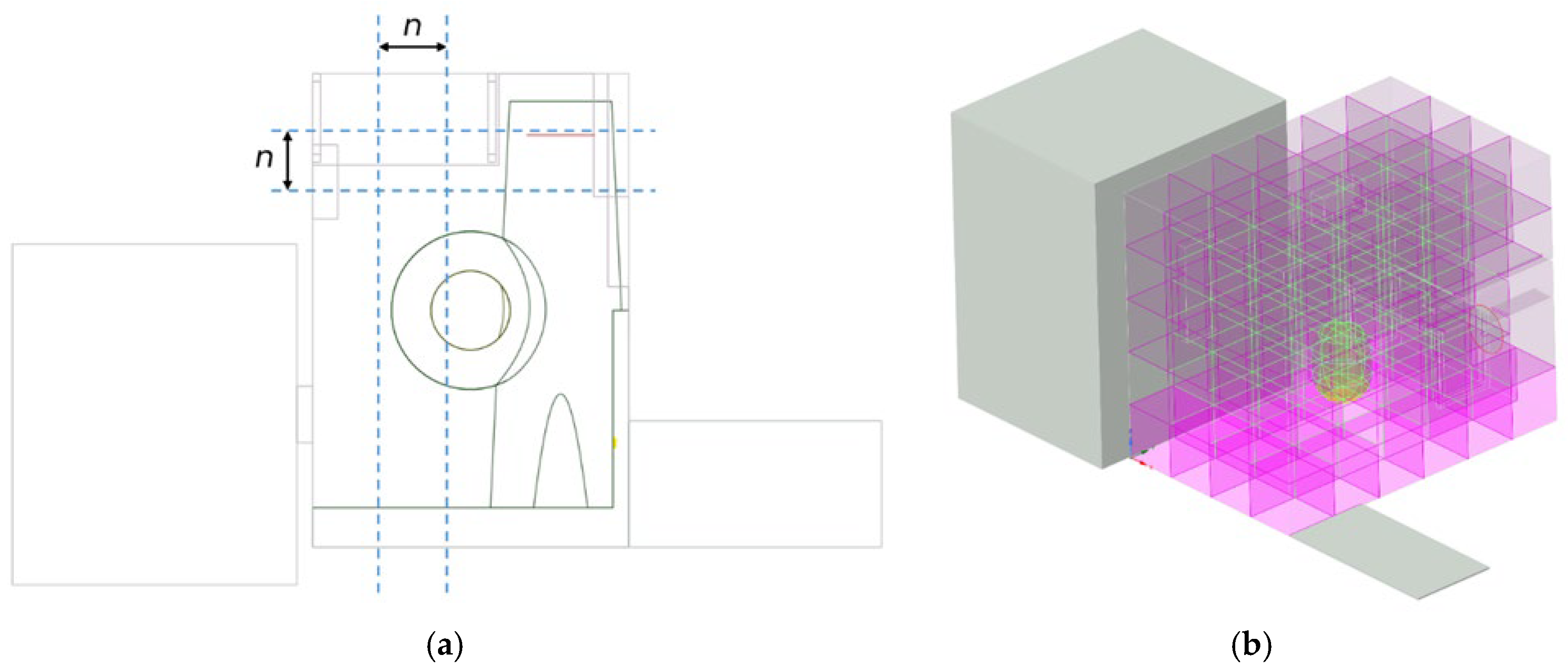
To identify suitable locations for PM sensors, the main volume of the bedroom is divided into a regular grid of cubic regions with side length n = 0.5 m. For the 2.0 × 3.0 × 2.5 m³ room, this yields 120 regions, shown in Figure 12. Four of these cubes intersect the fan disk. In the CFD model, these four cubes are merged into a single control volume to avoid interfering with the fan boundary condition. For post-processing, the same concentration history from this merged control volume is assigned back to the four corresponding region indices, so the exposure analysis formally uses 120 regions but only 117 of them are independent.

Figure 12. Room (a) spatial subdivision diagram and (b) 3D geometry. In (b), the magenta cubes denote the spatial regions used for the exposure analysis, while the translucent gray volume denotes the extension domains.

For each region, the CFD post-processing extracts a time series of volume-averaged PM concentration over the first 60 min of the simulation. Beyond 60 min, the concentrations are already close to ambient and add little information for sensor placement. The regional time series are grouped by height layer (z = 0–0.5, 0.5–1.0, 1.0–1.5, 1.5–2.0, 2.0–2.5 m) and reshaped into 4 × 6 matrices. Within a given layer, regions are referenced by their x-y indices shown on the heatmap axes and denoted as region (x,y) (e.g., region (1,2) corresponds to x = 1, y = 2); the height layer is specified separately (e.g., ceiling region (1,2) for z = 2.0–2.5 m). For a given time instant, each matrix represents the instantaneous spatial distribution of PM within one horizontal layer. Heatmaps are generated from these matrices using a uniform color scale for all cases and times, so that direct visual comparison between models and snapshots is possible. The locations of the incense source and the table footprint are annotated on the plots to aid interpretation of how emissions and internal obstructions influence the evolving concentration field. The heatmaps are taken at representative times spanning the initial build-up, near-peak conditions, and the subsequent decay phase after the incense stopped burning.

To relate the spatially resolved CFD fields to sensor-placement decisions, exposure-based metrics are defined for each region r. For every simulation and pollutant, the post-processing extracted the regional time series C_r(t) over the first 60 min of the simulation, which covers the build-up and early decay phases relevant for mapping. The maximum concentration C_max,r is taken as the peak value of C_r(t) in this 0–60 min window, which represents a worst-case short-term level. The time-averaged concentration C_avg,r, representing cumulative exposure in that region, is defined as the arithmetic mean of C_r(t) over the same period.

For normalization, the full set of 120 cubic regions is considered. The global peak concentration for a given simulation, C_max,room, is defined as the maximum of C_max,r over all regions, and the room-mean time-averaged concentration, C_avg,room, is computed as the average of C_avg,r over all regions. The four cubes intersecting the fan volume have identical concentration histories and therefore do not affect the ranking even though they are counted separately. Normalized metrics are then obtained as follows:

$$C_{\mathit{max},r}^{\ast }=C_{\mathit{max},r}/C_{\mathit{max},\mathit{room}}$$

(2)

$$C_{\mathit{avg},r}^{\ast }=C_{\mathit{avg},r}/C_{\mathit{avg},\mathit{room}}$$

(3)

Regions with C^*_max,r close to unity experience peaks comparable to the room maximum, while C^*_avg,r > 1 indicates above-average cumulative exposure.

A single scalar for ranking potential sensor locations is obtained by combining the two normalized metrics into an exposure score:

$$E_r=0.5(C_{\mathit{max},r}^{\ast }+C_{\mathit{avg},r}^{\ast })$$

(4)

Assigning equal weight to short-term peaks and longer-term exposure. For each representative CFD model, regions are sorted by E_r to identify hotspot cells and candidate sensor locations. The exposure scores are then mapped back onto the three-dimensional room subdivision and plotted as layer-wise heatmaps. For a given model, the color bar is fixed between the highest exposure score in the room (maximum E_r) and the 12th-highest region of the model (P90), so that candidate sensor locations stand out as the warmest cells. Comparing these exposure score maps between models highlights regions that repeatedly emerge as high-exposure candidates across different particle sizes and varying emission and air-change rates.

2.4. Persistence Metrics from Particle Tracks

To quantify how long particles persist in specific regions beyond peak concentrations, two residence time-based metrics were computed from the Lagrangian particle tracks over the analysis window after particle release: the fraction of particles entering a region and the P90 residence time among entrants. Let p = 1, …, N_p index the tracked particles and r = 1, …, N_r index the spatial regions shown in Figure 12.

2.4.1. Regional Residence Time

For each particle p, the residence time accumulated in r is the following:

$${\tau }_{p,r}={\int }_0^{T}1\left[x_p\left(t\right)\in r\right]\mathrm{dt}$$

(5)

where T = 3600 s and 1[⋅] is an indicator equal to 1 when the particle position, x_p(t), lies inside r. With discrete track output at times t_p,k, τ_p,r is evaluated by time-increment accumulation,

$${\mathsf{\tau }}_{p,r}\approx \sum _{k=1}^{K_p-1}∆t_{p,k}1\left[r_{p,k}=r\right]$$

(6)

$$∆t_{p,k}=t_{p,k+1}-t_{p,k}$$

(7)

where K_p is the number of recorded samples for p and r_p,k is the region containing the p at sample k.

2.4.2. Fraction of Particles Entering a Region

A particle is counted as an entrant to r if τ_p,r > 0. The entrant count and entrant fraction are

$$N_{\mathit{enter}}\left(r\right)=\sum _{p=1}^{N_p}1\left[{\mathsf{\tau }}_{p,r}>0\right]$$

(8)

$$f_{\mathit{enter}}\left(r\right)={\displaystyle \frac{N_{\mathit{enter}}\left(r\right)}{N_p}}$$

(9)

This metric captures how many particles ever reach a region during the analysis window.

2.4.3. P90 Residence Time Among Entrants

For regions with at least one entrant, the persistence of the upper tail is quantified using the 90th percentile of τ_p,r conditioned on entry:

$${\mathsf{\tau }}_{90,\mathit{enter}}\left(r\right)=Q_{0.90}\left(\left\{{\mathsf{\tau }}_{p,r}|{\mathsf{\tau }}_{p,r}>0\right\}\right)$$

(10)

Implemented as an order statistic: If the entrant times are sorted ascending as τ⁽¹⁾ ≤ … ≤ τ^(N_enter⁾, then

$${\mathsf{\tau }}_{90,\mathit{enter}}\left(r\right)={\mathsf{\tau }}^{\left(⌈0.90N_{\mathit{enter}}\left(r\right)⌉\right)}$$

(11)

This metric focuses on long-staying particles rather than the typical residence time. f_enter tells how many particles ever reach a region, while τ_90,enter tells how long they stay once they get there. Using both avoids treating a frequently visited region the same as a rarely visited region that traps particles for long periods.

3. Results and Discussion

3.1. Selection of Representative CFD Cases

From the 24 calibrated CFD models, four are selected for detailed analysis of particulate transport and spatial distribution: two for PM_2.5 (models 2.5-4A and 2.5-2B) and two for PM₁₀ (models 10-8A and 10-5B), with parameters detailed in Table 4. These cases span the range of air-change rates and emission parameters that still provide good agreement with experiments and therefore bracket the plausible behavior of the bedroom under the tested conditions. For PM_2.5, models 2.5-4A and 2.5-2B yield coefficients of determination R² = 0.9582 and 0.9435, respectively, when comparing CFD predictions to measured time series at the validation probes. For PM₁₀, models 10-8A and 10-5B achieve R² = 0.984 and 0.9771.

Table 4. DPM parameters of selected cases.

Case	Sim. Group	Emission Rate [µg/s]	Burning Time [min]	Inlet Mass-Flow Rate [kg/s]	Equivalent Air-Change Rate [ACH]
2.5-4A	PM2.5, z = 2.1 m	5.79	31	0.0098	1.96
2.5-2B	PM2.5, z = 1.5 m	4.60	34	0.02695	5.39
10-8A	PM10, z = 2.1 m	8.75	34	0.0147	2.94
10-5B	PM10, z = 1.5 m	10.69	34	0.0196	3.92

3.2. PM_2.5 Transport and Spatial Patterns

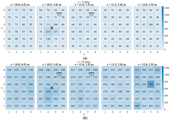
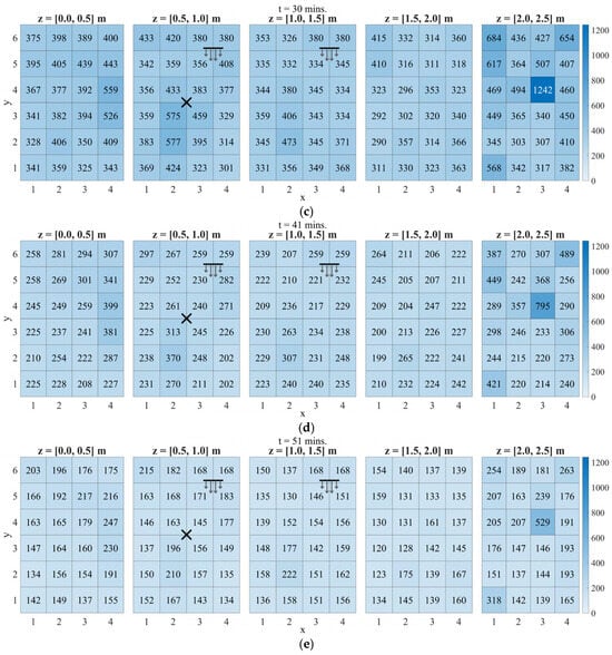
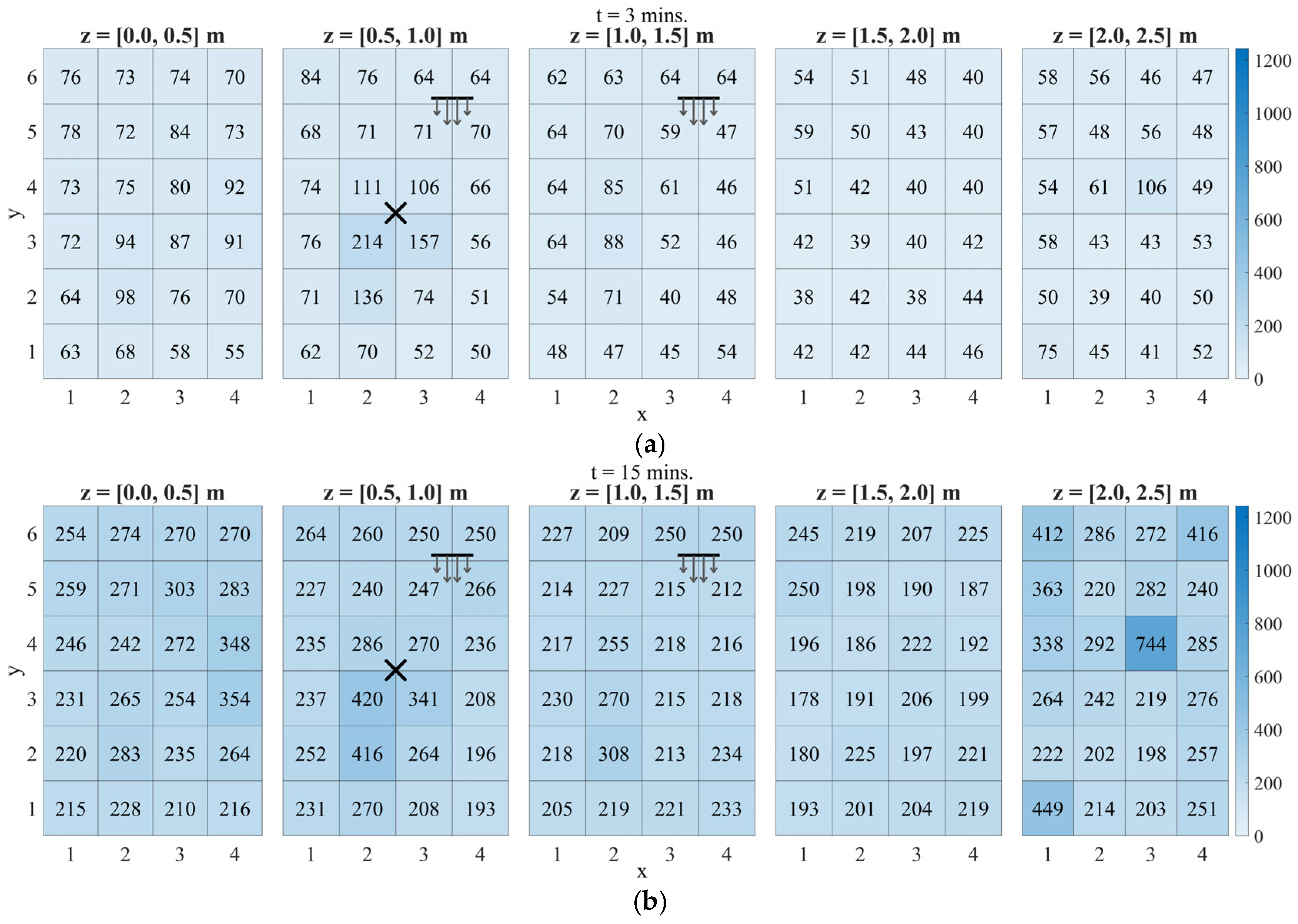
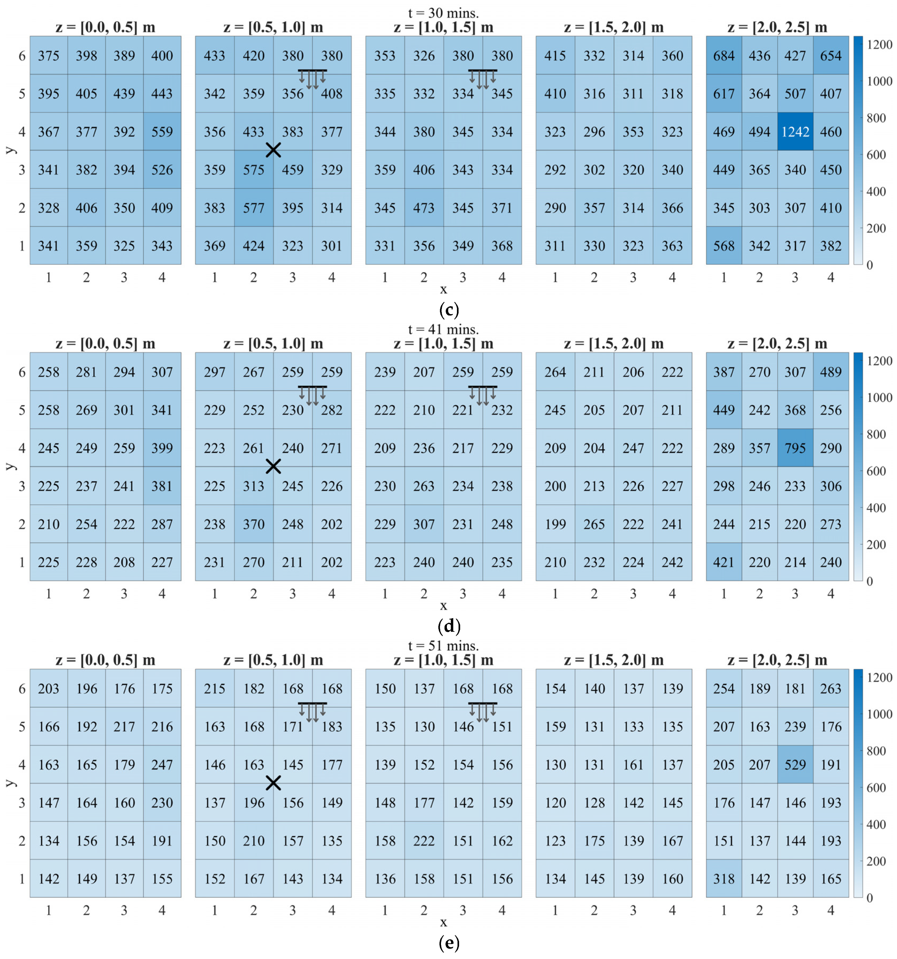
The PM_2.5 heatmaps for models 2.5-4A and 2.5-2B (z = 2.1 m and 1.5 m, respectively) show how the fan-driven circulation shapes the build-up and decay of fine particles in the bedroom. Figure 13 shows the heatmap snapshots of model 2.5-4A at t = 3, 15, 30, 41, and 51 min (a to e), illustrating the full evolution from the early emission phase to the late decay. Incense burning ends at t = 31 min. The elevation increases from left to right. The X-mark on the 2nd column (z = [0.5–1]) shows the location of the incense. The horizontal line on the 2nd and 3rd columns (z = [0.5–1] and z = [1–1.5]) represents the fan with the arrows showing the wind direction. At t = 3 min, high concentrations are strongly localized around the incense source, with the rest of the room otherwise comparatively uniform. By t = 15 min, the dominant hotspot has shifted to the uppermost layer (z = 2.0–2.5 m). This indicates rapid lofting and trapping in a ceiling-adjacent recirculation pocket. This hotspot is consistently anchored at ceiling region (3,4), which remains the global maximum through t = 30 min and persists as the highest-concentration pocket during the decay phase (t = 41 and 51 min). Near the end of burning (t = 30 min), this ceiling hotspot intensifies further and dominates the field. After the source is extinguished, concentrations decay across all layers, but the same ceiling region pocket persists as the maximum at t = 41 and 51 min, consistent with weak local exchange controlling the late-time removal.

Figure 13. PM_2.5 concentration heatmaps (in µg/m³) for model 2.5-4A at (a) t = 3, (b) 15, (c) 30, (d) 41, and (e) 51 min. The X mark denotes the incense source, and the horizontal line with arrows denotes the pedestal fan location and airflow direction.

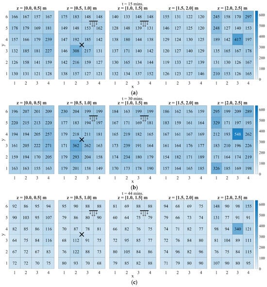
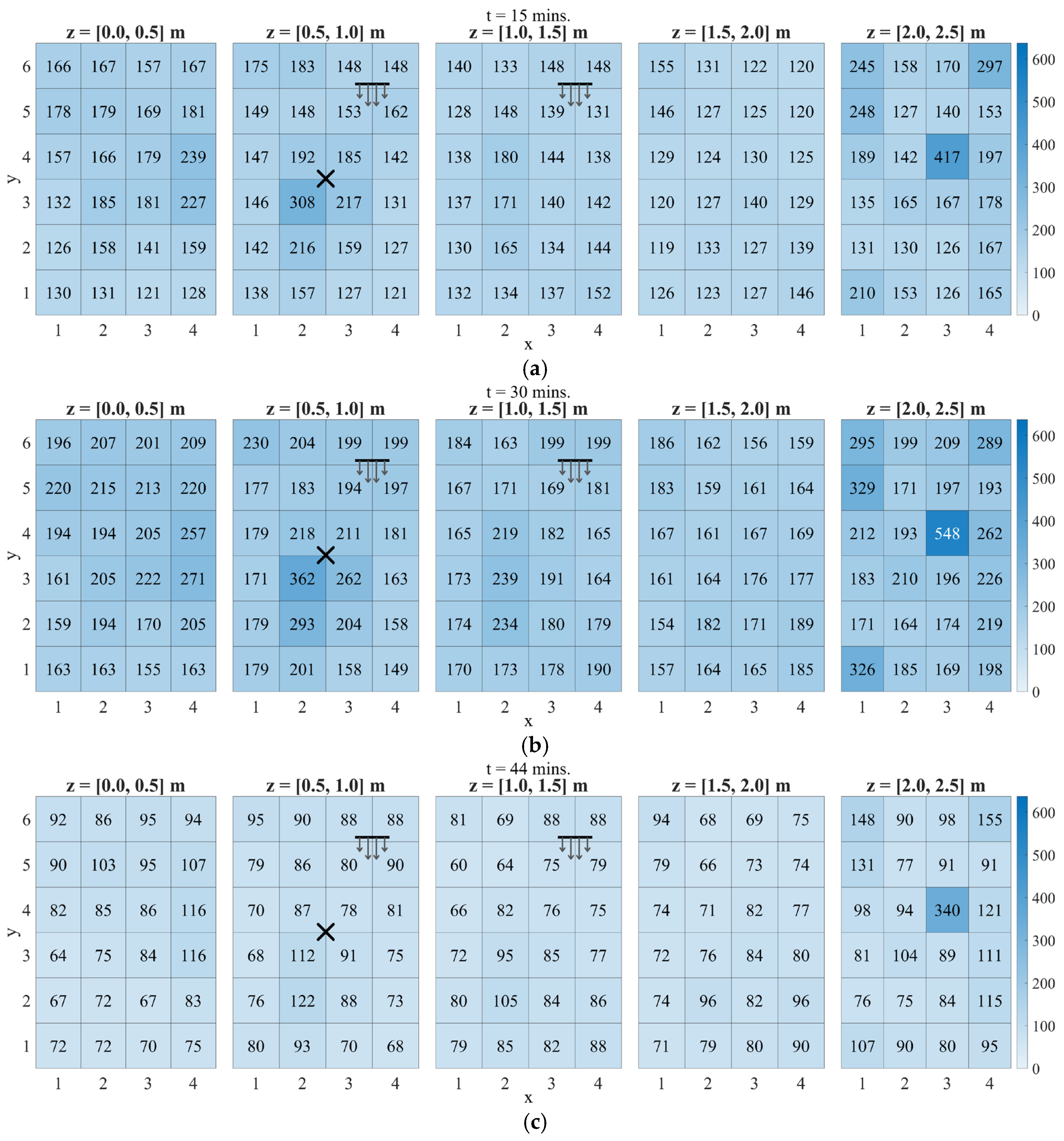
Figure 14 shows the heatmap snapshots of model 2.5-2B, which has a higher air-change rate and probes at z = 1.5 m, exhibiting the same dominant accumulation structure but at lower overall levels. Across all snapshots, the dominant hotspot remains ceiling region 34. Secondary build-ups are also evident in the ceiling corners, which suggests additional weakly ventilated zones near the perimeter at the top layer. At t = 15 min, the field is already non-uniform with emerging ceiling-layer enrichment; by t = 30 min, the ceiling hotspot intensifies while the rest of the domain remains comparatively moderate. During the decay phase (t = 44 min), concentrations drop across all layers, yet the same ceiling pocket remains elevated relative to the background with the weak local exchange controlling late-time removal. The main effect of the higher air-change rate is therefore a faster reduction in the room-wide concentration, not the removal of the persistent ceiling accumulation zone.

Figure 14. PM_2.5 concentration heatmaps (in µg/m³) for model 2.5-2B at (a) t = 15, (b) 30, and (c) 44 min. The X mark denotes the incense source, and the horizontal line with arrows denotes the pedestal fan location and airflow direction.

Taken together, the PM_2.5 cases highlight two key features of the bedroom relevant for monitoring: a near-source peak region where early-time concentrations are highest but highly sensitive to the exact source location, and persistent ceiling-level pockets, with elevated concentrations recurring in region 34 and the corners. After emissions cease, these ceiling pockets remain elevated while the rest of the room decays more uniformly. Any monitoring strategy that relies solely on measurements near the fan or close to the door/window is therefore at risk of underestimating PM_2.5 concentrations in these remote upper-corner regions.

3.3. PM₁₀ Transport and Spatial Patterns

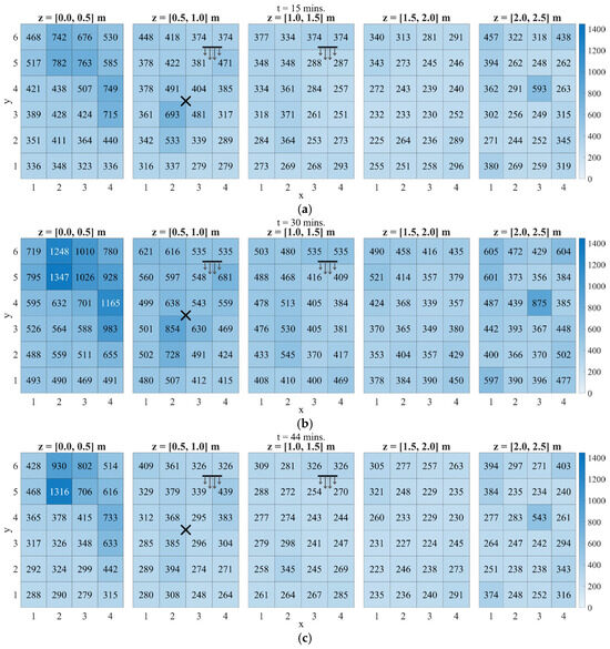
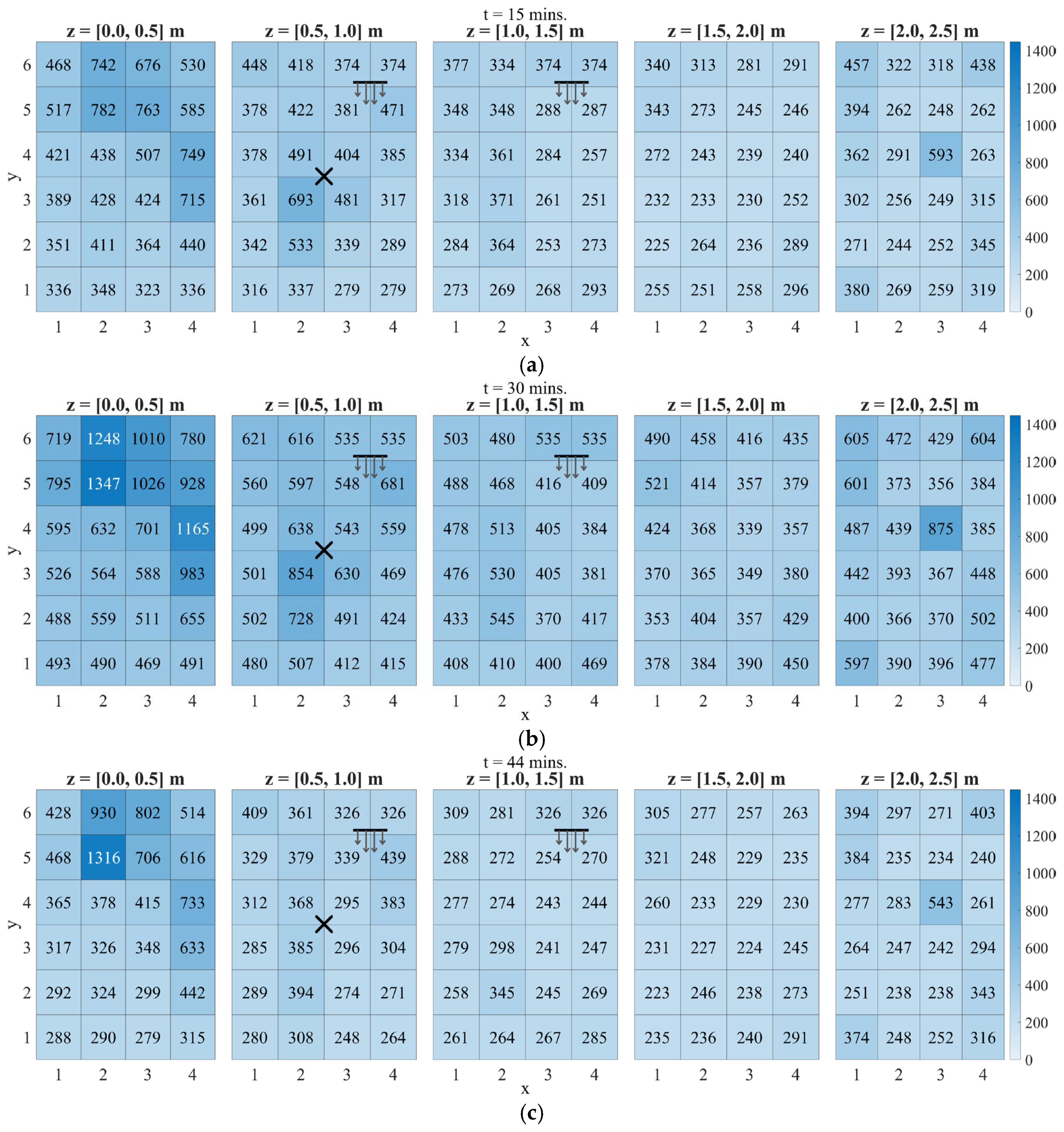
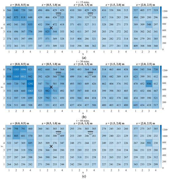
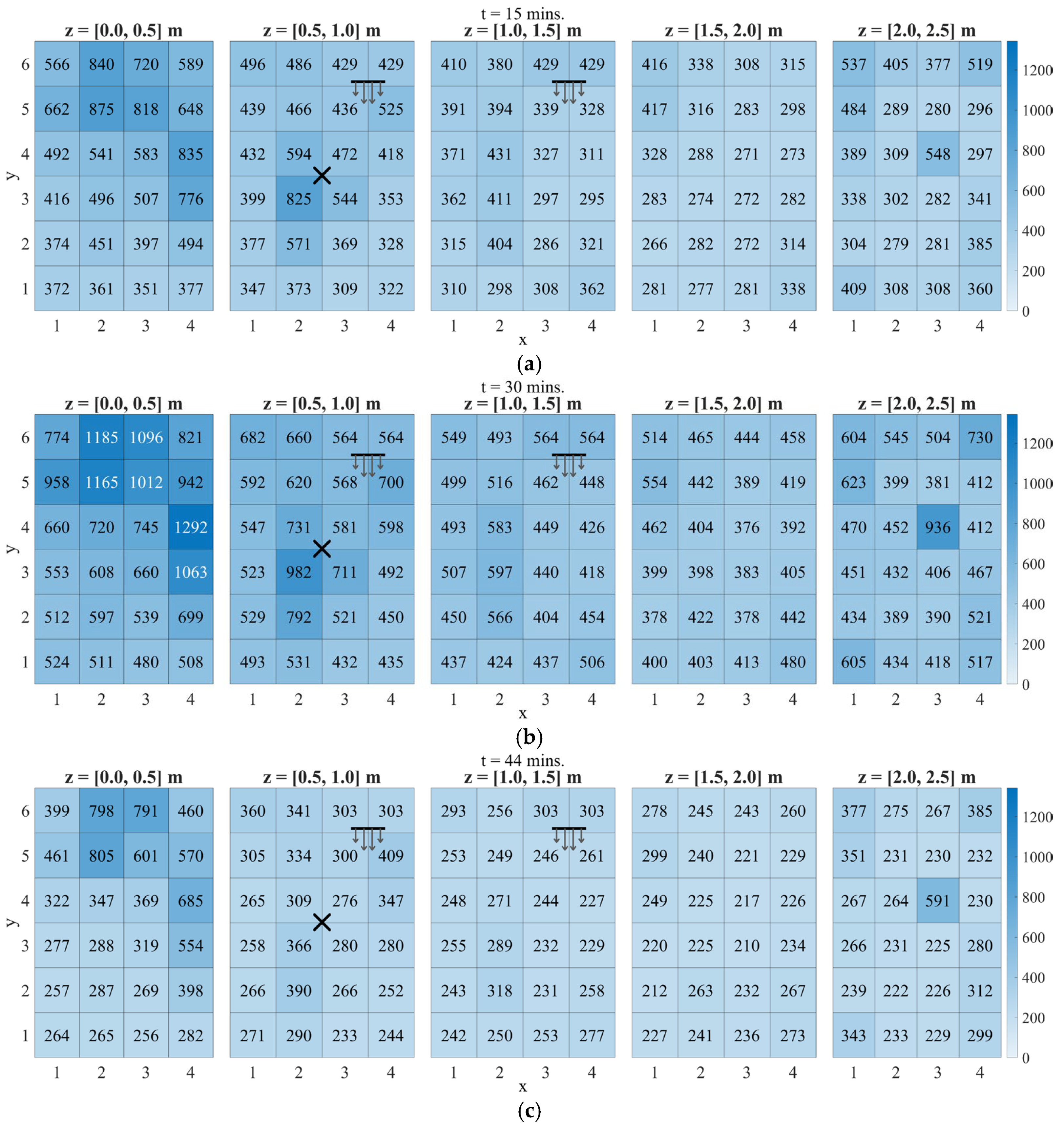
The PM₁₀ heatmaps for models 10-8A (z = 2.1 m) and 10-5B (z = 1.5 m) retain the same room-scale organization observed for PM_2.5, but the highest values sit more consistently in the lower layers. This distribution is consistent with gravity-enabled PM₁₀ transport, which increases floor accumulation relative to PM_2.5 while still allowing ceiling pockets to persist through recirculation. For model 10-8A in Figure 15, the t = 15 min snapshot concentrates around the source region and the floor layer. By t = 30 min, these near-floor pockets intensify, while the ceiling layer maintains a recurring hotspot at region (3,4). After the source is extinguished, concentrations decrease across all layers, yet the same floor and ceiling pocket locations remain visible at t = 44 min. Model 10-5B, in Figure 16, preserves the same pocket locations under a higher air-change rate: Decay is slightly faster, but residual hotspots persist in the floor layer and in ceiling pockets (region (3,4) and corners).

Figure 15. PM₁₀ concentration heatmaps (in µg/m³) for model 10-8A at (a) t = 15, (b) 30, and (c) 44 min. The X mark denotes the incense source, and the horizontal line with arrows denotes the pedestal fan location and airflow direction.

Figure 16. PM₁₀ concentration heatmaps (in µg/m³) for model 10-5B at (a) t = 15, (b) 30, and (c) 44 min. The X mark denotes the incense source, and the horizontal line with arrows denotes the pedestal fan location and airflow direction.

These PM₁₀ results reinforce the fact that the exposure field is driven by persistent pockets rather than by distance to the fan alone. Relative to PM_2.5, PM₁₀ exhibits stronger floor-layer gravity-enabled accumulation, while elevated ceiling pockets still recur at the same x-y locations, notably region (3,4) and the corners. While increasing the air-change rate mainly lowers the room-wide background and accelerates decay, the pocket locations remain. A single-point monitor placed near the fan or near openings can therefore miss both the floor accumulation zones and the ceiling pockets that control the late-time spatial contrasts.

3.4. Exposure Score Maps

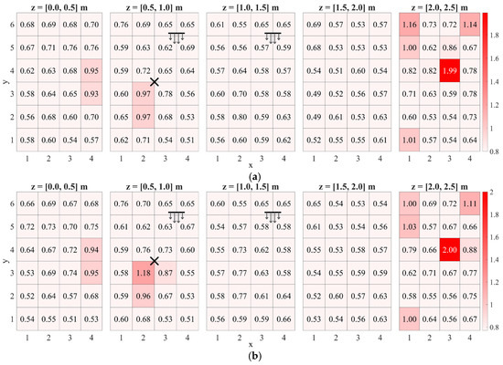
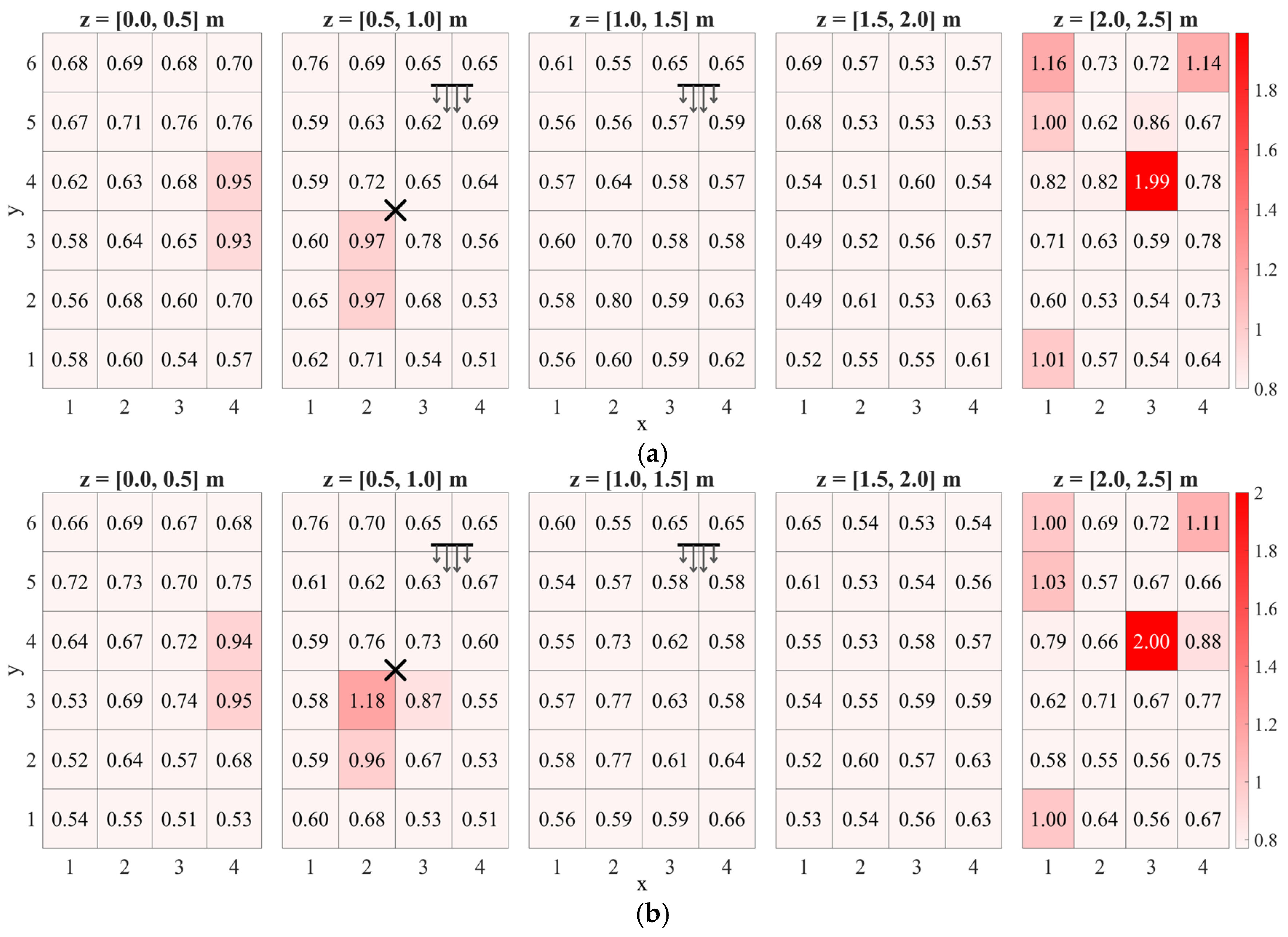
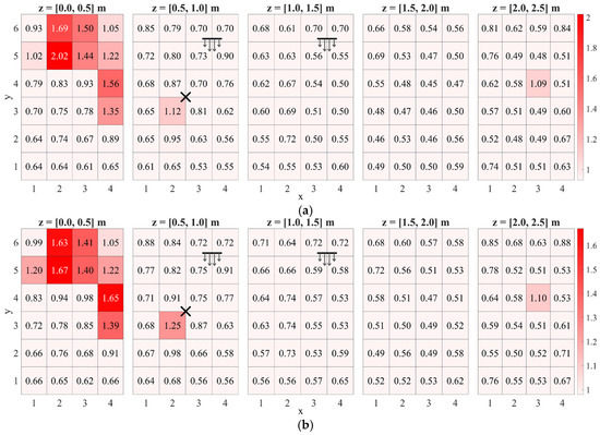
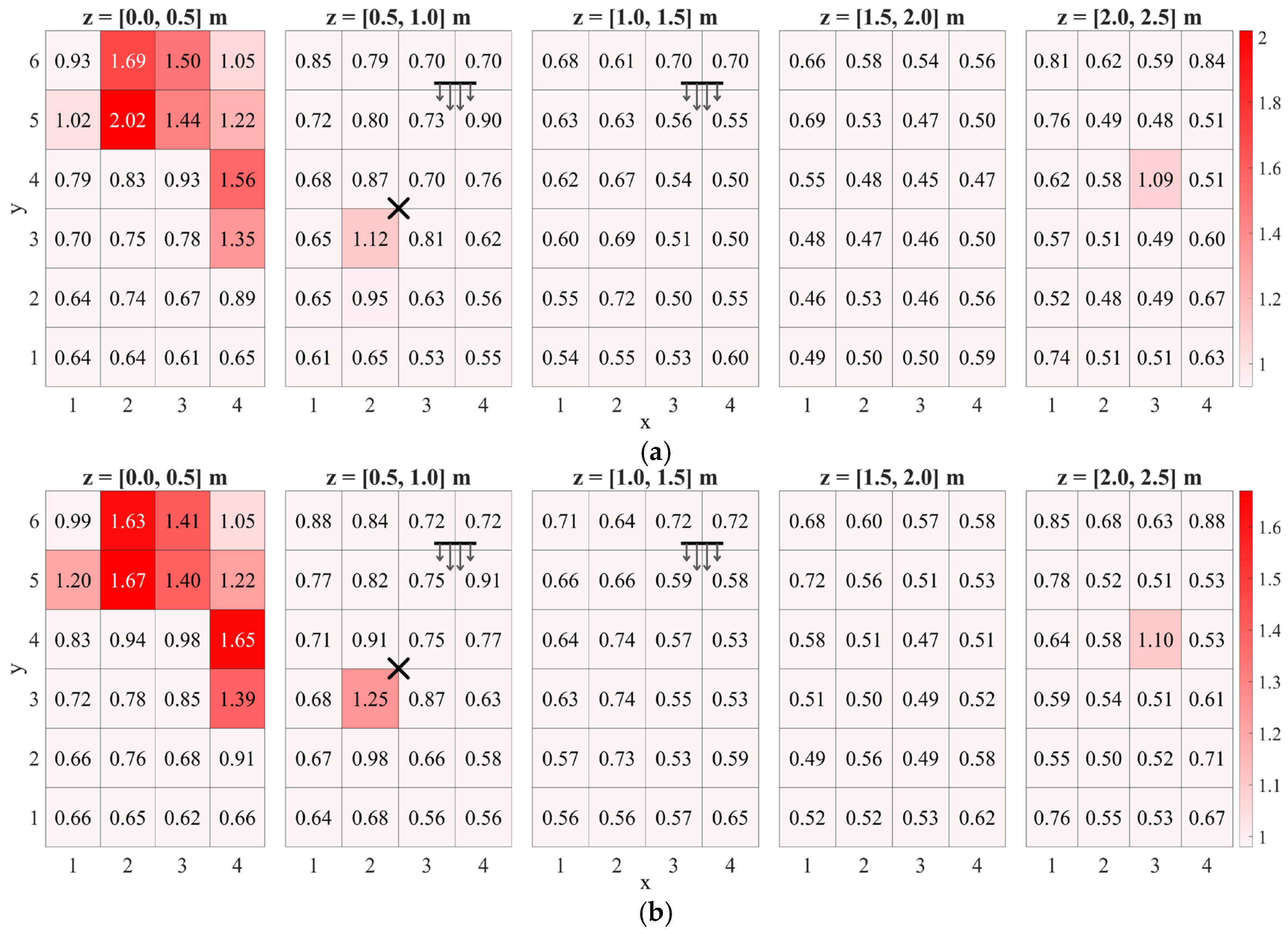
The exposure score E_r heatmaps for the PM_2.5 and PM₁₀ representative models summarize how peak and time-averaged PM levels combine across the room, as shown in Figure 17 and Figure 18, respectively. In all four cases, highest E_r concentrate in two parts of the room: floor-layer cells around the incense location, and a small set of ceiling-layer pocket cells, most visibly at ceiling region (3,4) and the corners. The balance between these two clusters shifts with particle size and air-change rate, but the hotspot locations repeat across the representative models.

Figure 17. Exposure score heatmap for models (a) 2.5-4A and (b) 2.5-2B. The X mark denotes the incense source, and the horizontal line with arrows denotes the pedestal fan location and airflow direction.

Figure 18. Exposure score heatmap for models (a) 10-8A and (b) 10-5B. The X mark denotes the incense source, and the horizontal line with arrows denotes the pedestal fan location and airflow direction.

At floor level, the cubes nearest the source register high E_r because they combine large early-time peaks with sustained elevated levels over the 1 h window. These cubes coincide with a low-speed region in the flow field, so particles are not rapidly swept into the main circulation. In the PM₁₀ exposure maps, the floor dominance is stronger: The top two P90-ranked regions occur at floor region (2,5) and floor region (4,4), whereas most other regions cluster near the background exposure score level.

The ceiling-layer hotspots are more localized but repeatable. For PM_2.5, ceiling region (3,4) is the room maximum in both E_r maps (≈2.0), with additional elevated cells in the ceiling corners. For PM₁₀, ceiling pockets remain present but with reduced intensity relative to the floor hotspots. The exposure score framework can be used as a quantitative basis for sensor-placement claims. However, in this study, it is used as an initial hotspot-screening metric, and its interpretation is complemented by additional parameters in the next sections.

3.5. Airflow Structure of High E_r Pockets

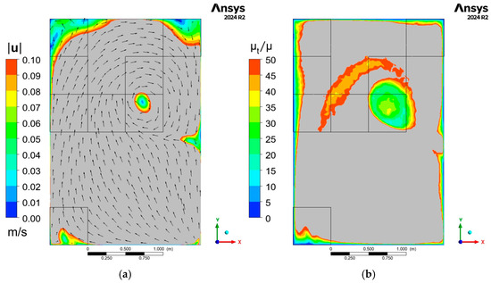
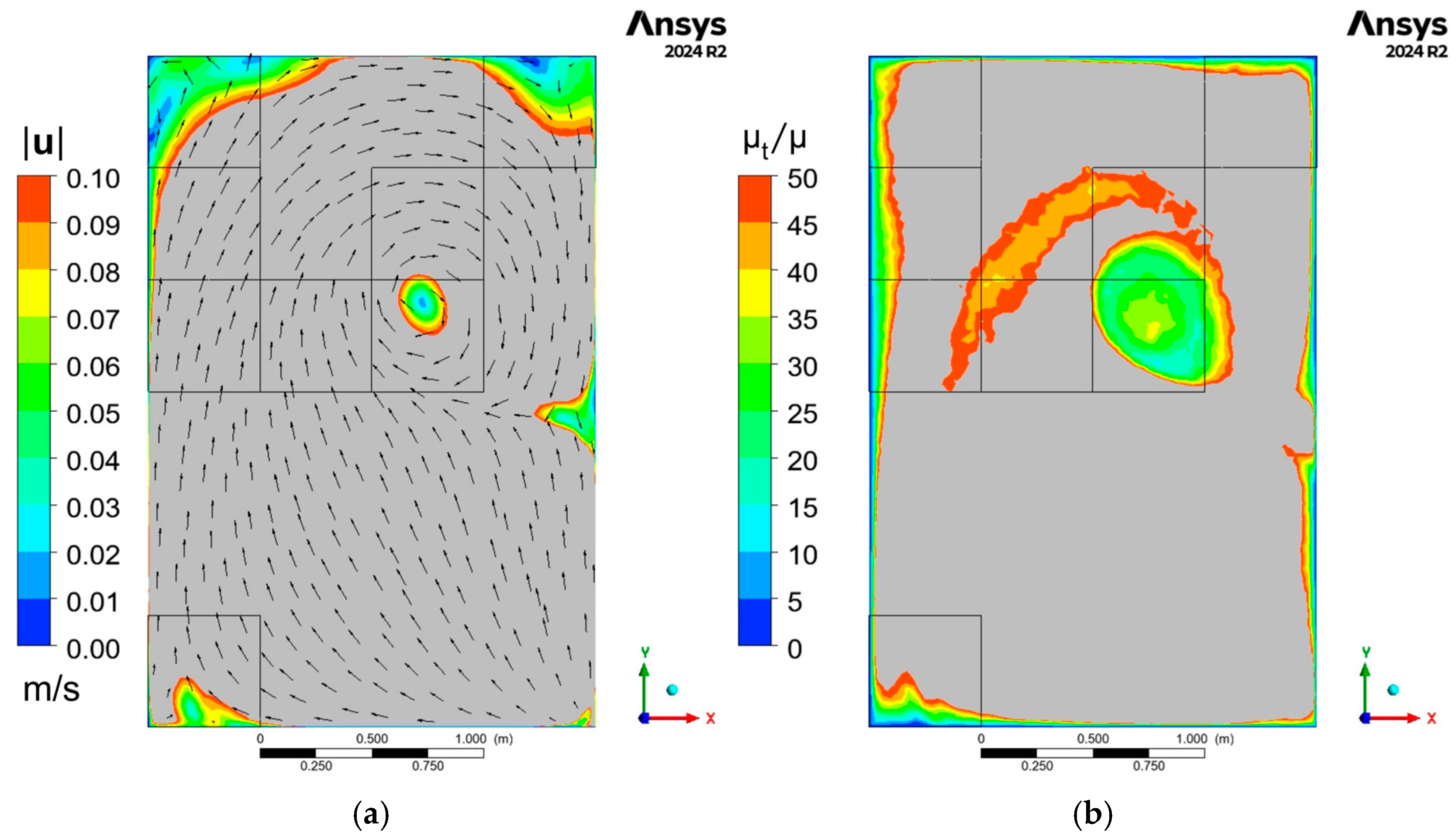
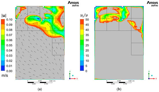
Figure 19 and Figure 20 show top-view contours of velocity magnitude, ∣u∣ (m·s⁻¹), and turbulent viscosity ratio, μ_t/μ. The P90 E_r region outlines are overlaid to locate the exposure hotspots within the spatial subdivision used in the heatmaps. Figure 19 is taken at z = 2.4 m (ceiling layer) and Figure 20 at z = 0.1 m (floor layer). These fields are extracted from the steady-state airflow solution and are therefore time-invariant over the PM transport window. The vectors on the ∣u∣ contours are single-colored and indicate flow direction only. Gray denotes values above the plotted maximum (clipped). For a given ventilation setting, the same ∣u∣ and μ_t/μ fields apply to both PM_2.5 and PM₁₀ cases because the discrete phase is simulated with one-way coupling.

Figure 19. Ceiling layer (z = 2.4 m) contours: (a) velocity magnitude (in m/s) with vectors and (b) turbulent viscosity ratio.

Figure 20. Floor layer (z = 0.1 m) contours: (a) velocity magnitude (in m/s) with vectors and (b) turbulent viscosity ratio.

At the ceiling plane, a compact low-∣u∣ pocket sits inside the cell that repeatedly appears as the PM_2.5 and PM₁₀ hotspot (ceiling region (3,4) in the heatmaps). In the same area, μ_t/μ drops as well. Low speed and low turbulent mixing limit exchange, so particles linger and the ceiling pockets persist during the decay phase. The band of higher μ_t/μ around the pocket traces the local shear layer. At the floor plane, low-∣u∣/low-μ_t/μ pockets appear along the perimeter and in localized recirculation zones. The highest PM₁₀ exposure regions fall on these same floor pockets. Settling is more prominent for PM₁₀, so the floor layer carries the strongest accumulation signal, while the pocket locations are set by the steady ventilation flow field rather than by distance to the source.

3.6. Persistence Metrics

Two residence time-based persistence metrics are investigated to characterize transport beyond peak concentrations. The fraction of particles entering a region, f_enter, measures reachability (how broadly a region is sampled by the released particles), while the 90th-percentile residence time among entrants, τ_90,enter, measures upper-tail retention (how long the long-staying particles remain once the region is reached). Because the exposure score maps show repeating hotspot locations across the representative PM_2.5 and PM₁₀ cases, models 2.5-4A and 10-8A are used here as illustrative persistence cases for the two particle-size classes. The same screening workflow may then be applied to other calibrated cases by ranking regions first by E_r and then checking f_enter and τ_90,enter to distinguish broadly sampled regions from true trapping pockets.

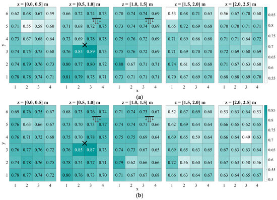
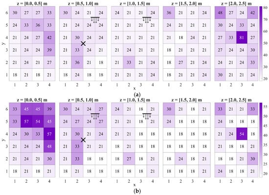
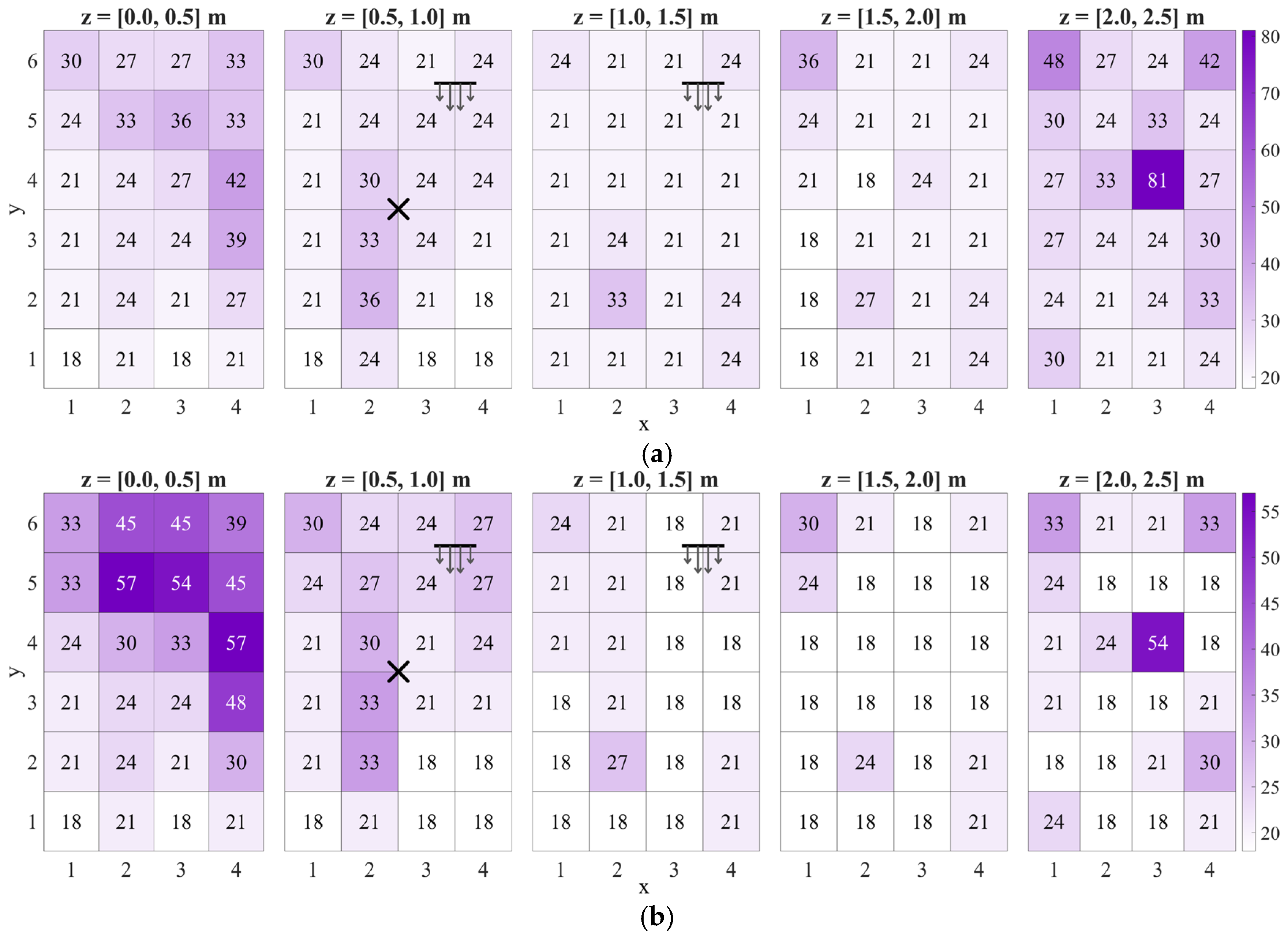
Figure 21 shows f_enter maps for models 2.5-4A and 10-8A. In both cases, reachability is highest in the source-adjacent circulation core: The z = 0.5–1.0 m layer contains the maxima, with f_enter ≈ 0.85–0.89 for PM_2.5 and 0.85–0.87 for PM₁₀ in the cells surrounding the source marker. Away from this core, most regions still register f_enter ∼0.6–0.75, so a majority of particles visit much of the room at least once during the 1 h window.

Figure 21. f_enter maps for models (a) 2.5-4A and (b) 10-8A. The X mark denotes the incense source, and the horizontal line with arrows denotes the pedestal fan location and airflow direction.

The main contrast between sizes appears in the uppermost layer. PM_2.5 maintains moderate reachability across the ceiling layer (typically ≳ 0.68), whereas PM₁₀ shows a clearer drop in ceiling reachability, including a minimum of about 0.49 in the ceiling hotspot cell. This is consistent with size-dependent settling: Fewer PM₁₀ trajectories reach the upper pockets, even though the airflow structure that defines the pocket locations is the same. f_enter therefore separates regions that are broadly sampled from regions that are weakly accessed.

Figure 22 displays the τ_90,enter maps for models 2.5-4A and 10-8A. In the PM_2.5 case, the largest upper-tail residence time occurs in the ceiling layer at region (3,4), where τ_90,enter reaches 81 s. Several other ceiling cells are elevated (order 30–50 s), while most regions in the middle layers sit closer to ~18–30 s. This separates the ceiling pocket behavior from the rest of the room: Once particles enter the pocket, a nontrivial fraction remains there for long residence times. In the PM₁₀ case, the strongest τ_90,enter values concentrate in the floor layer, with multiple hotspots reaching ~54–57 s. Upper layers are mostly ~18–27 s, and the ceiling pocket at region (3,4) remains visible (τ_90,enter = 54 s) but no longer dominates the map.

Figure 22. τ_90,enter maps (in seconds) for models (a) 2.5-4A and (b) 10-8A. The X mark denotes the incense source, and the horizontal line with arrows denotes the pedestal fan location and airflow direction.

Jointly, f_enter and τ_90,enter separate three behaviors. First, transit regions: high f_enter but modest τ_90,enter, where many particles pass through without long retention. Second, trapping pockets: moderate/low f_enter but high τ_90,enter, where entry is less frequent yet long-stay events dominate once particles arrive. Third, dominant accumulation zones: simultaneously high f_enter and high τ_90,enter, which combine broad access with long retention. The ceiling pocket illustrates the trapping-pocket behavior: For PM_2.5, ceiling region (3,4) has moderate reachability (~0.64) but the largest upper-tail residence time (81 s); for PM₁₀, the same cell is reached less often (down to ~0.49) yet still shows a long-stay tail (~54 s). In contrast, the PM₁₀ floor hotspots approach the dominant accumulation behavior by coupling relatively high reachability with elevated τ_90,enter.

A rank correlation check was performed to quantify how the exposure score E_r relates to the two persistence metrics. Spearman’s rank correlation, ρ_s, was computed across all 120 regions for the pairs (E_r,f_enter), (E_r,τ_90,enter), and (f_enter,τ_90,enter). This analysis does not replace the spatial maps but tests whether regions ranked high by E_r are also ranked high by reachability or upper-tail retention. As summarized in Table 5, E_r tracks τ_90,enter closely for both representative cases, whereas the association between E_r and f_enter is weaker and case-dependent. The relationship between f_enter and τ_90,enter also differs by case, showing that broad access and long-stay trapping can decouple depending on particle size and where the dominant accumulation layer forms.

Table 5. Spearman’s rank correlation between exposure score and persistence metrics.

Pair	Nused	2.5-4A		10-8A
		ρs	p	ρs	p
Er, fenter	120	−0.133	0.149	0.435	6.78 × 10−7
Er, τ90,enter	120	0.861	1.67 × 10−30	0.882	1.76 × 10−40
fenter, τ90,enter	120	−0.453	2.00 × 10−7	0.138	0.132

Table 5 motivates using the exposure score E_r as the primary screening metric for candidate monitoring locations because it aligns most closely with upper-tail retention τ_90,enter. The reachability metric f_enter provides a distinct check. It distinguishes broadly sampled regions from trapping pockets that can dominate exposure despite lower reachability. In the present bedroom and ventilation configuration, the PM_2.5 results consistently identify the ceiling pocket at region (3,4) as the most persistent hotspot (high E_r and high τ_90,enter), whereas the PM₁₀ results shift the dominant accumulation to the floor layer, where the top-ranked regions coincide with the floor hotspots. This implies that a single sensor location is insufficient to represent both particle sizes without bias; at minimum, a ceiling-pocket location (region (3,4)) should be paired with a floor-layer hotspot location.

4. Conclusions

This study developed and experimentally validated a transient indoor CFD framework for indoor particulate transport by coupling RANS airflow, buoyancy-enabled source representation, and Lagrangian discrete phase tracking in a full-scale bedroom with a fixed, non-oscillating pedestal fan and a window opening. The airflow solution was verified by grid-independence testing and validated against multi-point velocity measurements. The particulate phase model was subsequently calibrated and validated against experimental PM_2.5 and PM₁₀ time-series data which yields accepted cases with aggregate agreement above R² = 0.9. The validated transient PM transport fields were further translated into room-scale spatiotemporal maps that support objective-based guidance for candidate sensor placement.

Across the representative cases, the dominant PM patterns were governed primarily by airflow-defined accumulation pockets rather than by source proximity alone. Two recurrent behaviors emerged. First, a near-source region produced strong early-time peaks and remained sensitive to the exact source location. Second, remote recirculation pockets persisted in low-exchange zones and remained elevated during the decay phase. For PM_2.5, the most persistent hotspot was the ceiling-adjacent pocket at region (3,4), which combined high exposure score with the strongest upper-tail residence time behavior. For PM₁₀, the same room-scale airflow organization remained evident, but gravitational settling shifted the dominant accumulation toward floor-layer hotspots located in low-velocity, low-mixing zones. Changes in air-change rate mainly altered concentration magnitude and decay rate, but did not materially change the hotspot locations.

The exposure score framework proved useful as a first screening tool because it converts transient concentration histories into a simple spatial ranking that captures both short-term peaks and longer-term exposure. The added persistence metrics further strengthened the interpretation by separating broadly sampled transit regions from true trapping pockets. In particular, the strong association between exposure score and upper-tail residence time showed that the highest-ranked regions were not merely high because many particles passed through them, but because they preferentially retained long-staying particles. This gives the ranking a clearer physical basis for sensor-placement decisions.

From a monitoring standpoint, the results show that placement should follow the measurement objective. Near-source regions are more responsive to localized peak events, ceiling pockets are more suitable for persistent PM_2.5 hotspot monitoring, and floor hotspots are more critical for PM₁₀. Therefore, no single fixed sensor location is sufficient to represent both particle sizes without bias in the present bedroom configuration. At minimum, a ceiling-pocket location and a floor-layer hotspot location should be paired when the aim is to capture both persistent fine-particle retention and coarse-particle accumulation. More broadly, the study demonstrates that validated transient CFD, combined with exposure-based and persistence-based post-processing, can provide a physics-based workflow for translating non-uniform indoor PM transport into defensible sensor-placement guidance.

Future work should test the robustness of these rankings under different room sizes, source locations, ventilation operations, and window-door states, and should incorporate deposition and broader particle-size distributions to extend applicability to other indoor environments. It should also assess how the sensor-ranking results change under alternative weightings of peak and average concentration, as different monitoring objectives may prioritize short-term peaks, sustained exposure, or overall representativeness differently.

References

- Nassikas, N.J.; McCormack, M.C.; Kipen, H.M.; Balmes, J.R.; Bond, T.C.; Brigham, E.M.D.; Cromar, K.; Ewart, G.; Goldstein, A.H.; Hicks, A.; et al. Indoor Air Sources of Outdoor Air Pollution: Health Consequences, Policy, and Recommendations: An Official American Thoracic Society Workshop Report. Ann. Am. Thorac. Soc. 2024, 21, 365–376. [Google Scholar] [CrossRef] [Scilit]
- Izadyar, N.; Miller, W. Ventilation Strategies and Design Impacts on Indoor Airborne Transmission: A Review. Build. Environ. 2022, 218, 109158. [Google Scholar] [CrossRef] [Scilit]
- Liu, Y.; Ma, H.; Zhang, N.; Li, Q. A Systematic Literature Review on Indoor PM2.5 Concentrations and Personal Exposure in Urban Residential Buildings. Heliyon 2022, 8, e10174. [Google Scholar] [CrossRef] [Scilit] [PubMed]
- Silva, G.V.; Martins, A.O.; Martins, S.D.S. Indoor Air Quality: Assessment of Dangerous Substances in Incense Products. Int. J. Environ. Res. Public Health 2021, 18, 8086. [Google Scholar] [CrossRef] [Scilit] [PubMed]
- Park, S.; Song, D. CO2 Concentration as an Indicator of Indoor Ventilation Performance to Control Airborne Transmission of SARS-CoV-2. J. Infect. Public Health 2023, 16, 1037–1044. [Google Scholar] [CrossRef] [Scilit] [PubMed]
- Costanzo, V.; Yao, R.; Xu, T.; Xiong, J.; Zhang, Q.; Li, B. Natural Ventilation Potential for Residential Buildings in a Densely Built-up and Highly Polluted Environment. A Case Study. Renew. Energy 2019, 138, 340–353. [Google Scholar] [CrossRef] [Scilit]
- Lopes, M.B.; Kanama, N.; Poirier, B.; Guyot, G.; Ondarts, M.; Gonze, E.; Mendes, N. A Numerical and Experimental Study to Compare Different IAQ-Based Smart Ventilation Techniques. Buildings 2024, 14, 3555. [Google Scholar] [CrossRef] [Scilit]
- Concilio, C.; Aguilera Benito, P.; Piña Ramírez, C.; Viccione, G. CFD Simulation Study and Experimental Analysis of Indoor Air Stratification in an Unventilated Classroom: A Case Study in Spain. Heliyon 2024, 10, e32721. [Google Scholar] [CrossRef] [Scilit]
- Mathew, J.; Subbaiyan, G. Investigation of Ventilation Performance to Improve the Indoor Air Quality of Institutional Kitchens. J. Daylight. 2024, 11, 39–54. [Google Scholar] [CrossRef] [Scilit]
- Zhang, Q.; Li, L.; Zhou, J.; Braham, W.W.; Ma, N. A Spatial Analysis of Ozone and PM2.5 Distribution for Assessing Design Factors of Healthy Buildings. J. Build. Eng. 2024, 89, 109357. [Google Scholar] [CrossRef] [Scilit]
- Hsu, C.N.; Tsai, Y.L. Experimental Measurement and Computational Simulation Analysis of Indoor Air Quality in Office-Integration of Voltage Adsorption Dust Collection Device and Energy Recovery Ventilator. Sens. Mater. 2020, 32, 4299–4321. [Google Scholar] [CrossRef] [Scilit]
- Liu, Z.; Pfrang, C.; Sommariva, R.; Brean, J.; Su, Y.; Bloss, W.; Fraga, B. A Coupled Fluids-Chemistry Model for Pollutant Dynamics Indoors—Application to a Kitchen Scenario. Phys. Fluids 2025, 37, 053336. [Google Scholar] [CrossRef] [Scilit]
- Yun, S.; Licina, D. Optimal Sensor Placement for Personal Inhalation Exposure Detection in Static and Dynamic Office Environments. Build. Environ. 2023, 241, 110459. [Google Scholar] [CrossRef] [Scilit]
- Yun, S.; Zhong, S.; Alavi, H.S.; Alahi, A.; Licina, D. Proxy Methods for Detection of Inhalation Exposure in Simulated Office Environments. J. Expo. Sci. Environ. Epidemiol. 2023, 33, 396–406. [Google Scholar] [CrossRef] [Scilit]
- Ciuzas, D.; Prasauskas, T.; Krugly, E.; Sidaraviciute, R.; Jurelionis, A.; Seduikyte, L.; Kauneliene, V.; Wierzbicka, A.; Martuzevicius, D. Characterization of Indoor Aerosol Temporal Variations for the Real-Time Management of Indoor Air Quality. Atmos. Environ. 2015, 118, 107–117. [Google Scholar] [CrossRef] [Scilit]
- Hong, G.; Liao, C.; Liu, H. Study of Indoor PM2.5 Distribution Characteristics and Optimal Location for Its Monitoring in an Office. In Proceedings of the E3S Web of Conferences; EDP Sciences: Les Ulis, France, 2019; Volume 80. [Google Scholar]
- Yao, C.; Lee, S.; Kim, T. A Numerical Study on the Optimal Placement of Two Air Purifiers for Simultaneous Operation in a School Classroom. Int. J. Air-Cond. Refrig. 2025, 33, 6. [Google Scholar] [CrossRef] [Scilit]
- Anyaegbuna, B.E.; Onokwai, A.O.; Anyaegbuna, N.T.; Iweriolor, S.; Anyaegbuna, I.D.; Adegun, I.K.; Fayomi, O.S.; Ighravwe, D.E.; Onifade, M.K. Numerical Analysis on Mechanical Ventilation Impact on Indoor Air Quality in a Basement. Sci. Afr. 2024, 25, e02310. [Google Scholar] [CrossRef] [Scilit]
- Considine, B.; McNabola, A.; Kumar, P.; Gallagher, J. A Numerical Analysis of Particulate Matter Control Technology Integrated with HVAC System Inlet Design and Implications on Energy Consumption. Build. Environ. 2022, 211, 108726. [Google Scholar] [CrossRef] [Scilit]
- Zhao, X.; Wang, S.; Li, P.; Shi, X. Long-Term Indoor Air Quality Monitoring in Office Buildings: Data-Driven and Goal-Oriented Recommendations for Sensor Placement and Sampling Frequency. Build. Environ. 2025, 283, 113392. [Google Scholar] [CrossRef] [Scilit]
- Talami, R.; Hu, X.; Dawoodjee, I.; Ghahramani, A. Examining Different Placement Strategies for Indoor Environmental Quality Sensors in Office Environments. Sci. Technol. Built Environ. 2025, 31, 786–805. [Google Scholar] [CrossRef] [Scilit]
- Heemstra, T.; van der Schans, M.; Gibas, J.; Linnartz, J.P.M.G.; Delnoij, R. Ceiling-Mounted CO2 Sensing: Effect of Location and Stratification Temperature. Indoor Air 2024, 1840021. [Google Scholar] [CrossRef] [Scilit]
- Cheng, J.C.P.; Kwok, H.H.L.; Li, A.T.Y.; Tong, J.C.K.; Lau, A.K.H. BIM-Supported Sensor Placement Optimization Based on Genetic Algorithm for Multi-Zone Thermal Comfort and IAQ Monitoring. Build. Environ. 2022, 216, 108997. [Google Scholar] [CrossRef] [Scilit]
- Hu, X.; Zhang, M.; Fan, F. Numerical Investigation of Indoor Particle Behaviors in Different Ventilation Scenarios. Aerosol Air Qual. Res. 2025, 25, 35. [Google Scholar] [CrossRef] [Scilit]
- Vouriot, C.V.M.; van Reeuwijk, M.; Burridge, H.C. Uncertainties in Exposure Predictions Arising from Point Measurements of Carbon Dioxide in Classroom Environments. J. R. Soc. Interface 2024, 21, 20240270. [Google Scholar] [CrossRef] [Scilit]
- Guo, Q.; Tian, J.; Huang, R.; Boyce, C.M. Towards Accurate Modeling of Vibration in CFD-DEM Simulations of Vibrated Gas-Fluidized Beds without Using a Moving Mesh. Chem. Eng. Sci. 2024, 298, 120445. [Google Scholar] [CrossRef] [Scilit]
- Termini, S. CFD Modelling of the Pneumatic Conveying of Non-Conventional Solids; Politecnico di Torino: Turin, Italy, 2022. [Google Scholar]
- Cloete, J.H.; Cloete, S.; Radl, S.; Amini, S. Evaluation of Wall Friction Models for Riser Flow. Powder Technol. 2016, 303, 156–167. [Google Scholar] [CrossRef] [Scilit]
- Derksen, J.J.; van den Akker, H.E.A.; Sundaresan, S. Two-Way Coupled Large-Eddy Simulations of the Gas-Solid Flow in Cyclone Separators. AIChE J. 2008, 54, 872–885. [Google Scholar] [CrossRef] [Scilit]
Disclaimer/Publisher’s Note: The statements, opinions and data contained in all publications are solely those of the individual author(s) and contributor(s) and not of MDPI and/or the editor(s). MDPI and/or the editor(s) disclaim responsibility for any injury to people or property resulting from any ideas, methods, instructions or products referred to in the content. |
© 2026 by the authors. Licensee MDPI, Basel, Switzerland. This article is an open access article distributed under the terms and conditions of the Creative Commons Attribution (CC BY) license.