


Abstract
This work addresses the need for efficient and reusable vector embeddings (VEs) for large-scale RDF Knowledge Graphs, focusing on the widely used DrugBank dataset. The study aims to reduce the computational burden and environmental impact associated with repeatedly generating embeddings for downstream tasks such as link prediction, clustering, and recommendation. To this end, embeddings are generated from the DrugBank Knowledge Graph—comprising over 3.6 million triples, more than 1.5 million entities, and 95 relations—using 25 models implemented in the PyKEEN framework. The dataset is processed into training, validation, and test splits, and embeddings of fixed dimensionality are produced for both entities and relations. The resulting representations are released in multiple formats, including full JSON files, class-partitioned subsets, and an efficient Parquet-based structure, to support scalable querying. Experimental evaluation demonstrates substantial improvements in access time and memory usage when using structured formats, particularly Parquet. Additionally, the study quantifies the carbon footprint of embedding generation, showing that distributing precomputed embeddings can reduce energy consumption by up to 99.37% compared to on-demand recomputation. Overall, the work provides a comprehensive, reusable resource that facilitates research while promoting computational efficiency and environmental sustainability.
Dataset: https://zenodo.org/records/20714497 (accessed on 30 August 2026)
Dataset License: CC BY-NC 4.0
1. Summary
The current spread and success of sub-symbolic processing of symbolic information like RDF1 data presumes the availability of a multi-dimensional numerical representation of entities and the relations between them, commonly referred as vector embeddings (VEs), which sub-symbolic methods are applied to. Such VEs are then fed in downstream processing, e.g., in the case of RDF data, for link prediction [1], clustering [2], and Knowledge-aware Recommendation [3,4], just to name a few. More broadly, vector representations of graph-structured data are widely adopted beyond RDF and Knowledge Graphs, supporting tasks such as node classification and link prediction in social and information networks [5,6,7], as well as traffic forecasting in transportation networks [8] and intrusion detection in communication networks [9]. Due to the high variability in the application domains and in the embedding methods, off-the-shelf repositories of VEs are scarce, since the burden of their off-line computation can be amortized only by an intensive use of the very same VE among many (different) applications—the larger/more widespread the data store, the more convenient the VE pre-computation. This is the case for DrugBank, whose VEs we make available here for 25 different embedding methods.
However, the availability of off-line VEs for an RDF dataset is not just a time-saving facility for downstream applications; it may also be a benefit when considering the carbon footprint that stems from VE computation itself. In fact, while a significant reduction in computing time could also be obtained by using parallel architectures—which are now highly available even in a pay-per-use modality—such a time reduction would not reduce the power consumption needed to compute VEs, whose distributed computing among several devices does not reduce the total sum of the carbon footprint, and may even increase it [10]. In fact, some large open datasets [11] now also offer (along with symbolic data) the VEs of RDF resources, precomputed for a chosen VE model [12].
Since its first presentation [13], DrugBank has continued to represent a reference knowledge base for drugs, drug actions and drug targets, and it continues to be up to date [14]. Over 12,000 papers cited DrugBank in only the period from 2020 up to the present2. Therefore, both the widespread use of DrugBank and its continual maintenance qualify it as a target for an off-line computation of its VEs, which will be added into a dataset to be made available to researchers for intensive testing; this is not just a time-saving alternative to in-source computation, but more importantly an energy-saving alternative.
2. Data Description
The objective of this work is to provide a comprehensive collection of Knowledge Graph embeddings generated from the DrugBank Knowledge Graph introduced in Section 2.1. To support different data access strategies, the resulting embeddings are provided in multiple formats. Specifically, we release (i) complete embeddings for all entities and relations in the Knowledge Graph (Section 2.2), (ii) subsets of embeddings for selected DrugBank resource classes to facilitate exploration of the most relevant entities (Section 2.3), and (iii) a Parquet-based representation3 that enables efficient querying and scalable data access (Section 2.4). In addition, we report the estimated carbon footprint associated with the embedding generation process in Section 2.5.
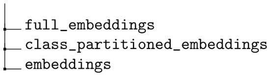
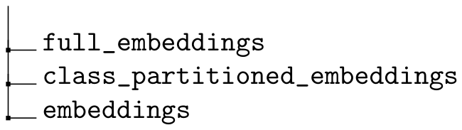
An overview of the directory structure of the released embeddings is presented in Figure 1, while the contents of each component are described in detail in the following sections.
Figure 1.
Directory structure of the released embeddings, organized into three main folders.
2.1. DrugBank
The embeddings provided in this work are generated from the DrugBank Knowledge Graph, using the last available RDF version as of 10 June 2026, namely version 34, provided by the Bio2RDF portal5 in N-Quads format [15]. Table 1 summarizes the main statistics of the Knowledge Graph, including the number of triples, entities, and relations. Each RDF triple is of the form , where s is the subject (also called the head), p the predicate, and o the object (tail). All resources in subject and object positions are treated as entities, while those in predicate positions are treated as relations.
Table 1.
Summary statistics of the DrugBank Knowledge Graph, including the number of triples, entities, and relations.
Among the entities, several DrugBank resource classes are particularly relevant for pharmacological and biological analysis, according to DrugBank statistics6. Table 2 reports the number of resources for each of these classes.
Table 2.
Number of resources for selected DrugBank resource classes.
2.2. Complete Knowledge Graph Embeddings
In general, we refer to the embeddings as representations, following the terminology adopted in the PyKEEN7 [16] library (v1.11.1) in a Python environment (v3.11), and use the two terms interchangeably, since each model may produce a single embedding or multiple embeddings for each entity or relation, or other types of information that are detailed in Section 3.1.1. Table 3 reports, for each model, the number of representations obtained for entities and relations—for example, AutoSF (first data row) uses four representations, both for the entities and for the relations. Consequently, the representations generated for each entity and relation in the dataset are stored in separate JSON files: one for entities and one for relations. These files are organized within the directory full_embeddings, according to the hierarchical structure illustrated in Figure 2, where model denotes the name of the Knowledge Graph embedding model.
Table 3.
Number of representations generated by each Knowledge Graph embedding model for entities and relations.
Figure 2.
Directory structure of the full_embeddings folder, where representations for entities and relations are stored in separate JSON files for each Knowledge Graph embedding model.
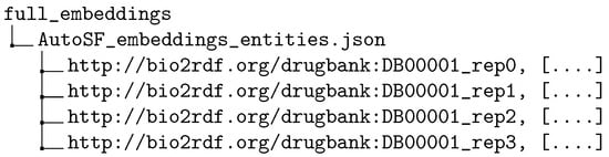
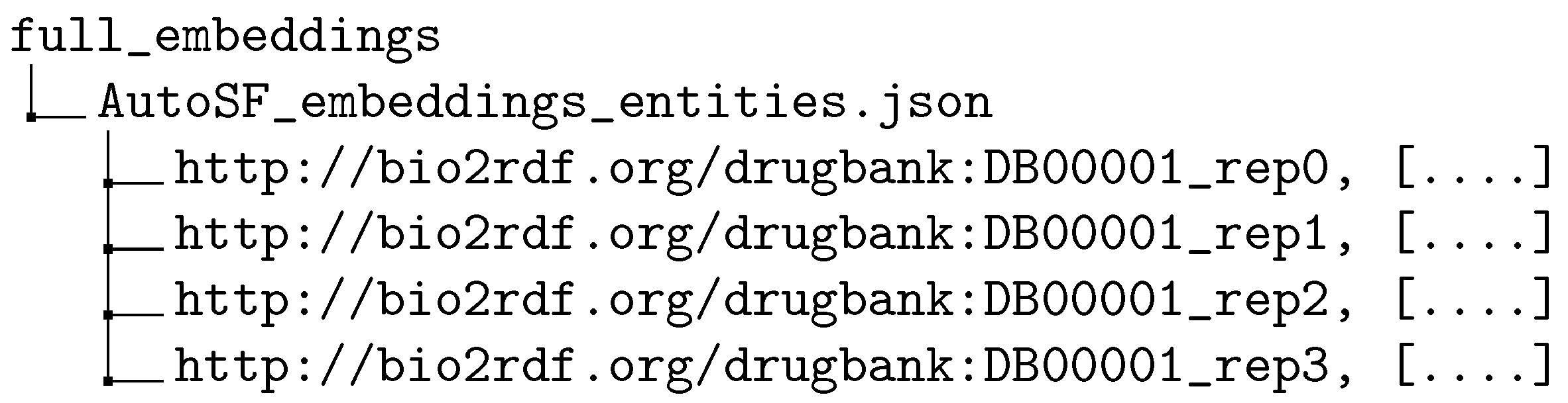
Representations in the JSON files are stored as key-value pairs. The JSON key corresponds to the id (URI or literal) of the entity or relation if the model generates a single representation per entity/relation and id_repn if the model generates multiple representations (with for the first representation, for the second, and sequential increments for additional representations). The values associated with each key correspond to the respective representation. For example, the AutoSF model produces four representations for each entity, as shown in Table 3. Therefore, for the entity “http://bio2rdf.org/drugbank:DB00001” (accessed on 10 June 2026), the JSON file would include four entries, one for each representation, as illustrated in Figure 3.
Figure 3.
Example of JSON entries for models producing multiple representations per entity or relation. Each list corresponds to the vector representation associated with the key.
Consequently, for models that generate multiple representations per entity or relation, the total number of entries in the JSON file is equal to the number of entities or relations multiplied by the number of representations produced by the model.
Furthermore, in the case of multiple representations, within each JSON file all resources associated with representation rep0 appear first, followed by those associated with rep1, and so on. By contrast, the CrossE model generates only one representation for each entity. Therefore, the JSON structure contains a single entry for each entity, as illustrated by the example in Figure 4.
Figure 4.
Example of JSON entries for models producing a single representation per entity or relation.
It should be noted that some resources may appear in both the entity and relation JSON files, since the same URI can occur in the Knowledge Graph both as an entity and as a relation. However, the relation JSON file (full_embeddings/model _embeddings_ relations.json) contains the representation(s) corresponding specifically to cases where that resource appears as a predicate in the Knowledge Graph. Similarly, the entity JSON file (full_embeddings/model _embeddings_entities.json) contains the representation(s) for resources appearing as subjects or objects.
2.3. Class-Partitioned Embeddings
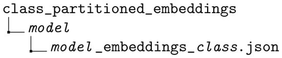
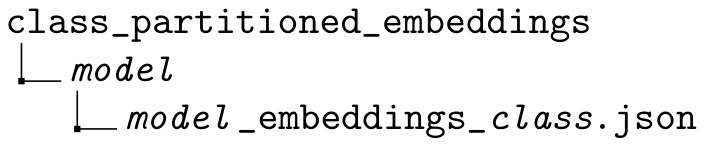
For completeness we provide the full entity JSON file for each Knowledge Graph embedding model (full_embeddings/model _embeddings_entities.json) to enable exploration of all entity representations in the Knowledge Graph, as described in Section 2.2. However, since these files are large and difficult to explore (ranging in size from approximately 3 to 13 GB), we additionally provide separate JSON files for each Knowledge Graph embedding model corresponding to the specific entity resource classes reported in Table 2. These files are organized according to the hierarchical structure shown in Figure 5, where each file follows the naming convention model _embeddings_class.json.
Figure 5.
Structure of the class_partitioned_embeddings directory, with JSON files containing representations for specific DrugBank resource classes.
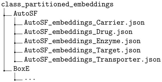
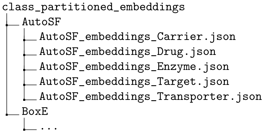
For instance, for the model AutoSF, the directory structure is illustrated in Figure 6.
Figure 6.
Example directory structure for the AutoSF model, showing JSON files for each DrugBank resource class (Carrier, Drug, Enzyme, Target, Transporter). Each file contains entity representation(s) corresponding to the specific class.
The format of these JSON files follows the same conventions described in Section 2.2 regarding keys, values, and representations.
2.4. Embeddings in Parquet Format
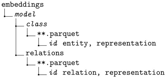
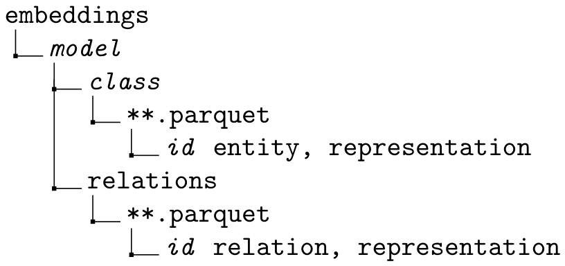
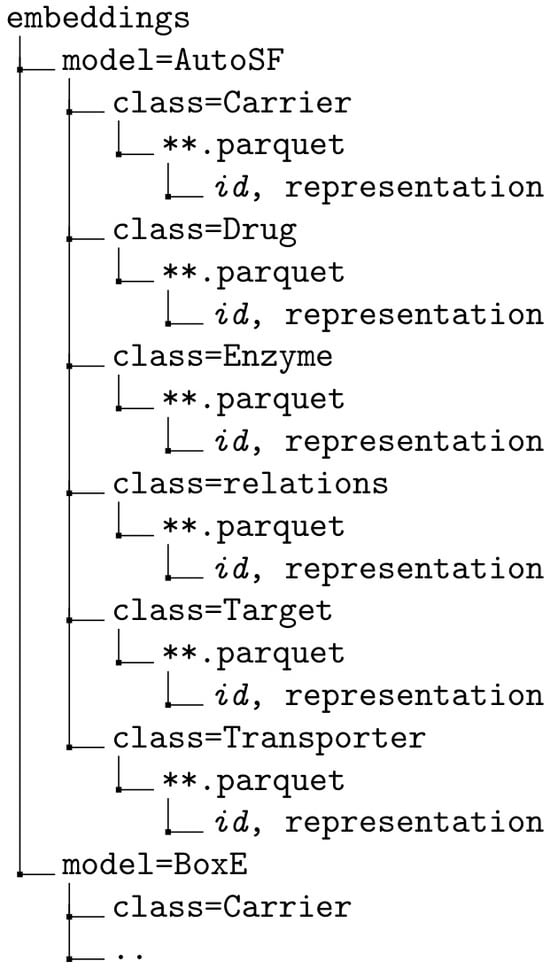
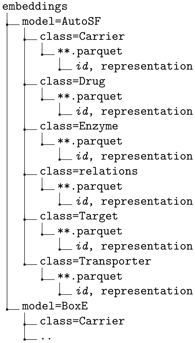
To further improve accessibility and facilitate exploration of the representations, we also provide them in Parquet format, partitioned by model and by the selected DrugBank resource classes, including representations for relations. The Parquet dataset, named embeddings, follows the general hierarchical structure shown in Figure 7, with a more detailed example illustrated in Figure 8.
Figure 7.
General hierarchical structure of the Parquet dataset, organized by model and by DrugBank class, containing representations for entities and relations. The notation **.parquet denotes the Parquet file contained in each corresponding class directory.
Figure 8.
Example of the Parquet dataset organization for the AutoSF model. The notation **.parquet denotes the Parquet file contained in each corresponding class directory.
The id follows the same naming convention introduced in Section 2.2: it corresponds to the entity or relation id when a single representation is provided and to entity/relation id_repn when multiple representations are available.
2.5. Carbon Footprint
Energy consumption, computed as the sum of CPU, GPU, and RAM energy, and the corresponding CO2 emissions for the embedding generation process are estimated using the CodeCarbon8 Python library (v3.2.1). The estimation considers experiments conducted in Italy on a device equipped with a 12th Gen Intel Core i7-12700F processor (2.10 GHz, 12 cores), an NVIDIA GeForce RTX 4060 Ti GPU, 64 GB of RAM, and a 2TB Kingston SNV2S2000G SSD. The results are reported in Table 4.
Table 4.
Runtime (in hours), CO2 emissions (in kilograms of CO2), and total energy consumption (in kilowatt-hour) measured during the embedding generation process using the 25 models. The final row summarizes the total values aggregated across all models and is shown in bold to distinguish it from the individual model results.
To provide an intuitive interpretation of the measured emissions, we use the equivalence provided by CodeCarbon9. According to these estimates, driving a European passenger car emits on average approximately 0.12 kgCO2 per kilometer under normal driving conditions. By summing the emissions generated by all the evaluated models, the total carbon footprint of our experiments corresponds approximately to driving a car for ≈178 km. Considering the same estimates, the total energy consumption of the embedding generation experiments corresponds to approximately 468 days of television usage, assuming an average daily usage of 6.5 h and a modern television with a power consumption of 21.2 W per hour (about 138 Wh per day). This is equivalent to about 3040 h (or ≈127 days) of continuous television operation.
Of course, the above carbon footprint estimations suffer from some local conditions—geographic location, computing facilities, etc.—that would hamper the use of such data outside the situations in which they were measured. Hence, to measure a more general “off-line download vs. on-line recomputation” gain, we also computed, in the same local conditions, the carbon footprint of the download of the VEs (i.e., full_embeddings.json in compressed format) and the Energy Gain ratio between the two measures. In this way, the Carbon Intensities () of the two footprints cancel out in the ratio, leaving a percentage gain that does not depend on local conditions. Then, by multiplying such a ratio for the local Carbon Intensity, a researcher may evaluate an absolute carbon footprint saving estimate for their own local conditions. The obtained results, aggregated across all models, are reported in Table 5. They show that downloading precomputed embeddings enables an energy reduction of approximately 158 times, corresponding to a reduction in carbon footprint—both in terms of emissions and total energy—of about 99.37%, independently of the geographic location.
Table 5.
Energy Gain ratio computed between the energy consumption of on-line recomputation and that of off-line download, aggregated across all models.
3. Methods
3.1. Embedding Generation
Embeddings are generated for each entity and relation in the DrugBank Knowledge Graph using 25 different models implemented in the PyKEEN library (v1.11.1). The original dataset is first processed by extracting all triples and converting them into TSV format. The resulting dataset is then randomly split at the triple level into training, validation, and test sets, using proportions of 90%, 5%, and 5%, respectively, while ensuring that all entities and relations occur at least once in each split. The training split is larger than usual because the produced embeddings are conceived and validated for unsupervised tasks, where labeled values are not available for validation and testing. The code used to perform the split is provided in the same repository as the dataset to support reproducibility. Embeddings are subsequently generated using the model-specific default hyperparameters provided by PyKEEN. According to the documentation10, these defaults are generally based on the best-performing values reported in the original publication introducing each model. The embedding dimensionality (d) is the only hyperparameter explicitly set to 100 for every model, while the same pipeline configuration is used for all of them11. The value falls within the range frequently adopted by PyKEEN and is consistent with the previous literature [22,26,27,34]. To ensure reproducibility, random_state and random_seed hyperparameters are both set to 1 for the data splitting and embedding generation processes, respectively.
3.1.1. Model Representations
As mentioned previously, while some models generate a single embedding for each entity or relation, others produce multiple representations (Table 3). In this section, we describe the meaning and role of the different representations produced by each embedding model that generates more than one representation.
AutoSF
In the original paper [17], the authors split entity and relation embeddings into four vectors of equal dimensionality. Similarly, in the implementation provided by PyKEEN, the default value of the parameter num_components is set to four. In this work, the embedding size d is set to 100 for all models (as stated in Section 3.1); consequently, when using PyKEEN, each entity is associated with four representations, each of dimension 100. This unified representation is designed to encompass several scoring functions, such as DistMult [22], ComplEx [19], Analogy [41], and SimplE [32]. Specifically, this partitioning enables the model to capture two key structural variations: (i) the distinction between real-valued and complex-valued embeddings, and (ii) the different ways in which split embeddings are combined by various scoring functions. By default, the use of four partitions enables the model to encompass the four aforementioned scoring functions while ensuring a tractable search space [17].
BoxE
Entities are modeled as points in Euclidean space and relations as boxes. Each entity is represented by two d-dimensional vectors: the first defines the base position of the entity, while the second represents a translational bump that shifts all entities co-occurring in a triple with this entity from their base positions to their final embeddings. Each relation is represented by n hyper-rectangles, where n corresponds to the arity of the relation r [18]. In the implementation provided by PyKEEN, the arity is always set to two (one box for the head position and one for the tail position), since the library only considers single-hop link prediction. As shown in Table 3, BoxE uses six relation representations. Specifically:
- The first (which we denote as rep0) is a d-dimensional vector and defines the box center for entities in the head position.
- The second (rep1) is a d-dimensional vector and defines the normalized extent of the head box along each dimension (i.e., the extents sum to one).
- The third (rep2) consists of a one-dimensional vector defining a scalar global scaling factor for the head box.
- The fourth (rep3) is a d-dimensional vector and defines the box center for entities in the tail position.
- The fifth (rep4) is a d-dimensional vector and defines the normalized extent of the tail box along each dimension.
- The sixth (rep5), like the third representation, is a one-dimensional vector and represents a scalar global scaling factor for the tail box.
CrossE
Each entity and relation is represented by two d-dimensional representations: a general embedding, which encodes high-level properties, and an interaction embedding, which captures specific features arising from crossover interactions [20]. When using PyKEEN, it is possible to obtain a single d-dimensional embedding per entity, while for relations, both representations are provided.
KG2E
This model represents each entity and relation as a Gaussian distribution, parameterized by two d-dimensional vectors: the first is a mean vector, which denotes its position in the embedding space, and the second a diagonal covariance vector, which models the (un)certainty associated with entities and relations. In this context, the (un)certainty of an entity or relation reflects the confidence in capturing its semantic meaning when scoring a triple [1].
MuRE
Each entity is represented by a d-dimensional embedding vector and two scalar bias terms, corresponding to its role as a head or as a tail in a triple, respectively. These bias terms determine the radius of a hypersphere decision boundary centered at the subject embedding after relation-specific transformation. In particular, the subject embedding and the object embedding are predicted to be related by relation r if the relation-adjusted object embedding falls within a hypersphere of radius . Each relation is represented by two representations: a d-dimensional relation offset vector, which models a translation from the subject to the object entity embeddings, and a diagonal relation matrix [25]. In the PyKEEN implementation, the latter is represented as a d-dimensional vector.
NTN
Each entity is modeled using a d-dimensional embedding vector. The model is designed to determine whether two entities participate in a relation R by computing a relation-specific scoring function [26]. In the implementation provided by PyKEEN, each relation is represented through the parameters of this scoring function, resulting in five distinct representations (see Table 3):
- The first (rep0) corresponds to the tensor layer and has dimensionality , where k is the number of tensor slices. By default, PyKEEN sets ; thus in our case this representation has a size of .
- The second (rep1) and third (rep2) correspond to the matrix , which is split in PyKEEN into two matrices of size , associated with the head and tail entities, respectively (in our case ).
- The fourth (rep3) and fifth (rep4) are vectors of dimension k (by default ): rep3 represents the bias vector, while rep4 corresponds to the final projection vector.
PairRE
Entities are modeled using a single d-dimensional embedding, while each relation is represented by a pair of d-dimensional representations. The first projects the head entity into Euclidean space while the second projects the tail entity [27].
SE
A single d-dimensional embedding is learned to model each entity, and two representations are learned for each relation, corresponding to the head and tail roles, respectively. These relation representations are modeled by PyKEEN as matrices, consistent with the original formulation [31].
SimplE
Each entity is represented by two d-dimensional vectors: one capturing the entity’s behavior when it appears as a subject and the other when it appears as an object. Similarly, each relation is represented by two d-dimensional vectors: one for the relation itself and one for its inverse [32].
TransD
This model represents each entity and relation with two d-dimensional vectors: one capturing the meaning of the entity or relation, and the other serving as a projection vector that determines how to project an entity embedding into the corresponding relation vector space [34]. In the implementation provided by PyKEEN, it is possible to define different dimensionalities for entity and relation embeddings. However, by default, these dimensions are set to be equal, and in our experiments we keep this default configuration, setting for both entities and relations.
TransH
Entities are modeled using a single d-dimensional embedding vector, while each relation is represented by two d-dimensional vectors. In the implementation provided by PyKEEN, the first corresponds to the relation-specific translation vector in the hyperplane and the second to the normal vector defining the relation-specific hyperplane (denoted as and , respectively, in the original notation [37]).
TransR
Each entity is modeled using a single d-dimensional embedding vector, while relations are represented in a distinct relation-specific entity space. Since the dimensionality of relation embeddings can differ from that of entity embeddings, in the default PyKEEN configuration the relation dimension (k) is set to 30, whereas we set the entity dimension to 100. Each relation is associated with two representations: the first is a k-dimensional vector corresponding to the relation embedding itself, while the second is a relation-specific projection matrix of size that projects entities from the entity space to the relation space [38]. As a result, the embeddings provided for this model have a dimensionality of 100 for entities and 30 for the first representation of relations, while the second representation of relations is a relation-specific projection matrix of size (i.e., shape ), which maps entity embeddings from the entity space to the relation space.
4. User Notes
The Parquet structure enables efficient access to the embeddings using analytical tools such as DuckDB [42]. In contrast to JSON files, which typically require loading large portions of data into the memory, the columnar and partitioned structure of Parquet allows selective access to the relevant subsets of the dataset. In particular, we compare three alternative access strategies: (i) using the complete JSON files containing all entity representations, (ii) using the class-partitioned JSON files that group representations by class, and (iii) querying the Parquet dataset through DuckDB (v1.4.3). To illustrate the advantages of the different formats provided in this work, we report three example queries. The execution time and memory usage12 for the three queries under the different access strategies are reported in Table 6.
Table 6.
Comparison of execution time (in seconds) and memory usage (in megabytes) for the three example queries under different data access strategies: full JSON embeddings, class-partitioned JSON files, and the Parquet dataset queried with DuckDB. Reported values correspond to the average over three independent runs.
- Query 1: Retrieving the representation(s) of a specific drug.The following example retrieves the representation associated with the drug “http://bio2rdf.org/drugbank:DB00001” (accessed on 30 August 2026) generated by the DistMA [21] model.
- When using the complete JSON embeddings file, the entire file full_embeddings/DistMA_embeddings_entities.json must be loaded in order to access the value corresponding to the key “http://bio2rdf.org/drugbank:DB00001” (accessed on 30 August 2026). This requires loading a file of approximately 3 GB.
- Using the class-partitioned JSON file reduces the amount of data that must be loaded. In this case, the required information can be obtained by loading the specific file class_partitioned_embeddings/DistMA/DistMA_embeddings_Drug.json (approximately 16 MB) and retrieving the value associated with the same key.
- Finally, when using the Parquet structure, the same result can be obtained by executing the following query using DuckDB:
- SELECT id, representation
- FROM read_parquet (’embeddings/∗∗’)
- WHERE model = ’DistMA’
- AND class = ’Drug’
- AND id = ’http://bio2rdf.org/drugbank:DB00001’;
- Query 2: Retrieving the representations for entities belonging to a specific DrugBank resource class.The following query retrieves all representations generated by the DistMA model corresponding to entities of the Target class.
- When using the full JSON representations file, retrieving all representations for a specific resource class (e.g., Target) requires prior knowledge of the target entities’ identifiers. In this case, the entire file containing all entity embeddings must be loaded and iterated over to identify the entries whose keys correspond to the target resources and extract the associated representations. In contrast, the other two access strategies do not require prior knowledge of the target identifiers.
- When using the class-partitioned JSON representation, the desired embeddings can be obtained simply by loading the file (e.g., class_partitioned_embeddings/DistMA/DistMA_embeddings_Target.json), which already only contains the representations for the resources belonging to the Target class.
- When using the Parquet representation, the same result can be obtained by executing the following query using DuckDB:
- SELECT id, representation
- FROM read_parquet (’embeddings/∗∗’)
- WHERE model = ’DistMA’
- AND class = ’Target’;
- Query 3: Retrieving the representation(s) of a specific drug across all models. This query aims to retrieve all embeddings corresponding to the drug with URI http://bio2rdf.org/drugbank:DB00001 (accessed on 30 August 2026) for each model.
- When using the complete JSON embeddings, the entire file containing all entity embeddings for each model (full_embeddings/model _embeddings_entities.json) must be loaded in order to access the value corresponding to the key http://bio2rdf.org/drugbank:DB00001 (accessed on 30 August 2026). This requires loading 25 files, with sizes ranging from approximately 3 GB to 13 GB.
- When using the class-partitioned JSON file, it is sufficient to load the specific file corresponding to the Drug class for each model (class_partitioned_embeddings/model/model _embeddings_Drug.json) and extract the representation(s) associated with the given URI. These files are significantly smaller than those in the previous access strategy, ranging in size from approximately 16 MB to 63 MB.
- When using the Parquet representation, the same result can be obtained efficiently by executing, for each model, the following query in DuckDB:
- SELECT id, representation
- FROM read_parquet (’embeddings/∗∗’)
- WHERE
- model = ’{model}’
- AND class = ’Drug’
- AND (id = ’http://bio2rdf.org/drugbank:DB00001’ OR
- id LIKE ’ http://bio2rdf.org/drugbank:DB00001_rep%’);
The three queries illustrate increasing levels of complexity. The first query retrieves the representation of a single entity for a single model, the second retrieves the representations of all entities belonging to a specific class for a single model, and the third retrieves the representation(s) of a single entity across all models. The results show a substantial improvement in performance when moving from a JSON representation to more structured storage formats. In the full embedding configuration, the entire dataset is loaded and processed regardless of the specific query requirements. This leads to very high execution times and memory usage, highlighting the inefficiency of scanning large JSON files when only a subset of the data is actually needed. The first major improvement is achieved with the class-partitioned JSON approach. By splitting the embeddings according to their class, queries can access only the relevant subset of the data. This significantly reduces both execution time and memory consumption. The best performance, particularly in terms of execution time, is obtained using the Parquet dataset queried with DuckDB. In fact, Queries 1 and 2 execute in tens of milliseconds, while Query 3 executes in hundreds of milliseconds. This corresponds to an order-of-magnitude improvement over the class-partitioned JSON approach, up to three-orders-of-magnitude improvement compared to the full embedding configuration for Queries 1 and 2, and reaching up to four orders of magnitude for Query 3. When using the Parquet representation, memory usage is significantly reduced for Queries 1 and 3 compared to the full embedding approach and is less than half of that required by the class-partitioned strategy. For Query 2, memory usage is slightly higher than that of the class-partitioned approach, while remaining comparable and still significantly lower than the full embedding configuration. Overall, we provide the Parquet representation as it offers the best trade-off between execution time and memory usage, enabling scalable and efficient querying even on large datasets. The full JSON embeddings may still be useful in cases of the representation of an entity that does not belong to the selected DrugBank classes.
5. Downstream Use Case: Unsupervised Learning
To illustrate the applicability of the released embeddings in downstream tasks, we consider an unsupervised learning scenario focused on DrugBank resources of type Drug. Specifically, for each embedding model, we use entity embeddings as input representations for clustering-based analysis. As explained in Section 3.1.1, different embedding models may generate different numbers and types of entity representations. Therefore, we apply a model-specific preprocessing step to obtain a single vector representation for each drug entity. For models that produce a single entity representation, we directly use the corresponding embedding. For complex-valued models such as ComplEx [19] and RotatE [30], we concatenate the real and imaginary parts of each embedding, following the common practice [19] of representing complex-valued embeddings as real-valued vectors. For models that learn multiple entity representations (AutoSF [17], BoxE [18], KG2E [1], SimplE [32], and TransD [34]), we concatenate the available representations to obtain a single vector per entity, thereby preserving all learned information in a unified representation. Finally, for MuRE [25], we use only the first entity representation, since the second and third learned components correspond to scalar bias terms.
5.1. Clustering Settings
We perform clustering using Hierarchical Agglomerative Clustering, setting only the distance metric, the linkage criterion, and the number of clusters (k), while keeping the remaining hyperparameters at their default values. We use cosine distance as the distance metric, since it is commonly adopted for vector embeddings [21,43,44]. We adopt average linkage, which computes inter-cluster distances by considering all pairwise distances between elements of the two clusters. This choice reduces the influence of individual outliers compared with single and complete linkages, which are determined by the closest and farthest pair of points, respectively. Ward linkage is excluded because it cannot be used in combination with cosine distance. The number of clusters k is determined through the Calinski–Harabasz index by selecting the value that maximizes the index within the predefined interval . This interval is intended to cover a sufficiently broad range of possible clustering solutions, while excluding configurations that are either too coarse or excessively fragmented. Given the number of resources considered in our experiments, and assuming approximately balanced clusters, this interval corresponds to an average cluster size ranging from about 13 to 95 resources.
5.2. Results
The results are reported in Table 7 in terms of overall cluster cohesion, measured through the average intra-cluster cosine distance. For each cluster with at least two elements, we compute the average pairwise cosine distance13 between all entities belonging to the cluster, thus quantifying how close the cluster elements are in the embedding space. The model-level score is then obtained by averaging these values over all clusters produced by the model. Since the score is distance-based, lower values indicate higher cohesion, meaning that the model produces, under the adopted settings, more geometrically compact clusters.
Table 7.
Optimal number of clusters and overall intra-cluster cosine distance obtained for each embedding model. Lower values indicate higher geometric cohesion of the clusters produced under the adopted clustering settings.
For this downstream task (clustering with hierarchical clustering), results guide the implementer towards vector embedding models showing better performance. Of course, for a different downstream task, the choice of the better models may change. In this respect, our repository provides a ready-to-use starting point for any downstream task starting from the vector embeddings of DrugBank data.
Author Contributions
Conceptualization, S.C., F.M.D. and V.S.; methodology, S.C., F.M.D. and V.S.; software, V.S.; validation, V.S.; investigation, S.C., F.M.D. and V.S.; resources, V.S.; data curation, V.S.; writing—original draft preparation, S.C., F.M.D. and V.S.; writing—review and editing, S.C., F.M.D. and V.S.; visualization, V.S.; supervision, S.C. and F.M.D.; funding acquisition, S.C. and F.M.D. All authors have read and agreed to the published version of the manuscript.
Funding
This work has been partially supported by the Italian aerospace technological district “Distretto Tecnologico Aerospaziale S.C.a.r.l.” and by project “LIFE: the itaLian system wIde Frailty nEtwork” founded by Ministry of Health (CUP D93C22000640001).
Data Availability Statement
The vector embeddings generated in this study are openly available on Zenodo at https://zenodo.org/records/20714497 (accessed on 30 August 2026) The embeddings are generated from the DrugBank RDF Knowledge Graph obtained from the Bio2RDF portal (https://download.bio2rdf.org/#/current/drugbank/ (accessed on 10 June 2026)). The original DrugBank data are third-party data and remain subject to the terms and conditions of the original data provider.
Conflicts of Interest
The authors declare no conflicts of interest.
Abbreviations
The following abbreviations are used in this manuscript:
| VE | Vector Embedding |
| CI | Carbon Intensity |
Notes
| 1 | https://www.w3.org/TR/rdf12-concepts/ (accessed on 30 August 2026). |
| 2 | Source: Scopus, queried with key term “DrugBank” on 15 January 2026; query with key terms “DrugBank and RDF” (respectively “DrugBank and BIO2RDF”) returns 122 (respectively, 60) documents in the same time range. |
| 3 | https://parquet.apache.org/docs/ (accessed on 30 August 2026). |
| 4 | https://download.bio2rdf.org/#/current/drugbank/ (accessed on 10 June 2026). |
| 5 | http://bio2rdf.org (accessed on 10 June 2026). |
| 6 | https://go.drugbank.com/stats (accessed on 30 August 2026). |
| 7 | https://pykeen.readthedocs.io/en/stable/ (accessed on 30 August 2026). |
| 8 | https://docs.codecarbon.io/latest/ (accessed on 30 August 2026). |
| 9 | https://docs.codecarbon.io/latest/introduction/methodology/#estimation-of-equivalent-usage-emissions (accessed on 30 August 2026). |
| 10 | The documentation states: “Each model’s default hyper-parameters were chosen based on the best reported values from the paper originally publishing the model unless otherwise noted on the model’s reference page.” |
| 11 | According to the PyKEEN 1.11.1 documentation, the default pipeline uses the stochastic Local Closed World Assumption (sLCWA), the RankBasedEvaluator, the Adagrad optimizer with an initial learning rate of 0.01, the BasicNegativeSampler, 5 training epochs, a batch size of 256, and no early stopping (see https://pykeen.readthedocs.io/en/v1.11.1/_modules/pykeen/pipeline/api.html#pipeline as of 9 July 2026). In addition, all models included in our experiments use the MarginRankingLoss with a ReLU margin activation. |
| 12 | Memory usage corresponds to the Resident Set Size measured using the psutil.Process.memory_info function from the psutil Python library (https://psutil.readthedocs.io (accessed on 30 August 2026)) (v7.2.1). |
| 13 | Hierarchical Agglomerative Clustering, the Calinski-Harabasz index, and pairwise distances are computed using the scikit-learn [45] (v1.6.1) implementation. |
References
- He, S.; Liu, K.; Ji, G.; Zhao, J. Learning to Represent Knowledge Graphs with Gaussian Embedding. In Proceedings of the 24th ACM International Conference on Information and Knowledge Management, CIKM ’15, Melbourne, Australia, 18–23 October 2015; pp. 623–632. [Google Scholar] [CrossRef] [Scilit]
- Colucci, S.; Donini, F.M.; Schena, V.; Scioscia, F.; Di Sciascio, E. LISE: A Logic-based Interactive Similarity Explainer for clusters of RDF data. IEEE Access 2025, 13, 90109–90128. [Google Scholar] [CrossRef] [Scilit]
- Anelli, V.W.; Ferrara, A.; Musto, C.; Narducci, F.; Ragone, A.; Zanker, M. Sixth Knowledge-aware and Conversational Recommender Systems Workshop (KaRS). In Proceedings of the 18th ACM Conference on Recommender Systems, RecSys ’24, Bari, Italy, 14–18 October 2024; pp. 1245–1249. [Google Scholar] [CrossRef] [Scilit]
- Zhang, J.C.; Zain, A.M.; Zhou, K.Q.; Chen, X.; Zhang, R.M. A review of recommender systems based on knowledge graph embedding. Expert Syst. Appl. 2024, 250, 123876. [Google Scholar] [CrossRef] [Scilit]
- Perozzi, B.; Al-Rfou, R.; Skiena, S. DeepWalk: Online learning of social representations. In Proceedings of the 20th ACM SIGKDD International Conference on Knowledge Discovery and Data Mining, KDD ’14, New York, NY, USA, 24–27 August 2014; pp. 701–710. [Google Scholar] [CrossRef] [Scilit]
- Grover, A.; Leskovec, J. node2vec: Scalable Feature Learning for Networks. In Proceedings of the 22nd ACM SIGKDD International Conference on Knowledge Discovery and Data Mining, KDD ’16, San Francisco, CA, USA, 13–17 August 2016; pp. 855–864. [Google Scholar] [CrossRef] [Scilit] [PubMed]
- Tang, J.; Qu, M.; Wang, M.; Zhang, M.; Yan, J.; Mei, Q. LINE: Large-scale Information Network Embedding. In Proceedings of the 24th International Conference on World Wide Web, WWW’15, Florence, Italy, 18–22 May 2015; pp. 1067–1077. [Google Scholar] [CrossRef] [Scilit]
- Yu, B.; Yin, H.; Zhu, Z. Spatio-temporal graph convolutional networks: A deep learning framework for traffic forecasting. In Proceedings of the 27th International Joint Conference on Artificial Intelligence (IJCAI’18), Stockholm, Sweden, 13–19 July 2018; pp. 3634–3640. [Google Scholar]
- Zhong, M.; Lin, M.; Zhang, C.; Xu, Z. A survey on graph neural networks for intrusion detection systems: Methods, trends and challenges. Comput. Secur. 2024, 141, 103821. [Google Scholar] [CrossRef] [Scilit]
- Lannelongue, L.; Grealey, J.; Inouye, M. Green algorithms: Quantifying the carbon footprint of computation. Adv. Sci. 2021, 8, 2100707. [Google Scholar] [CrossRef] [Scilit] [PubMed]
- Färber, M.; Lamprecht, D.; Krause, J.; Aung, L.; Haase, P. SemOpenAlex: The scientific landscape in 26 billion RDF triples. In Proceedings of the International Semantic Web Conference, ISWC’23, Athens, Greece, 6–10 November 2023; Springer: Berlin/Heidelberg, Germany, 2023; pp. 94–112. [Google Scholar] [CrossRef] [Scilit]
- Erten, Ö.; Mehryar, S.; Xiong, B.; Çelebi, R.; Brewster, C. Refining SemOpenAlex Concept Ontology: A Constraint-Aware Approach via Knowledge Graph Embeddings and SKOS Constraints. In Proceedings of the 15th International Conference on Semantic Web Applications and Tools for Health Care and Life Sciences, SWAT4HCLS 2024, Leiden, The Netherlands, 20–26 February 2024; pp. 56–65. [Google Scholar]
- Wishart, D.S.; Knox, C.; Guo, A.C.; Cheng, D.; Shrivastava, S.; Tzur, D.; Gautam, B.; Hassanali, M. DrugBank: A knowledgebase for drugs, drug actions and drug targets. Nucleic Acids Res. 2008, 36, D901–D906. [Google Scholar] [CrossRef] [Scilit] [PubMed]
- Knox, C.; Wilson, M.; Klinger, C.M.; Franklin, M.; Oler, E.; Wilson, A.; Pon, A.; Cox, J.; Chin, N.E.L.; Strawbridge, S.A.; et al. DrugBank 6.0: The DrugBank Knowledgebase for 2024. Nucleic Acids Res. 2023, 52, D1265–D1275. [Google Scholar] [CrossRef] [Scilit] [PubMed]
- Carothers, G. RDF 1.1 N-Quads. A Line-Based Syntax for RDF Datasets. W3C Recommendation 25 February 2014. 2014. Available online: https://www.w3.org/TR/n-quads/ (accessed on 30 August 2026).
- Ali, M.; Berrendorf, M.; Hoyt, C.T.; Vermue, L.; Sharifzadeh, S.; Tresp, V.; Lehmann, J. PyKEEN 1.0: A Python Library for Training and Evaluating Knowledge Graph Embeddings. J. Mach. Learn. Res. 2021, 22, 1–6. [Google Scholar]
- Zhang, Y.; Yao, Q.; Dai, W.; Chen, L. AutoSF: Searching Scoring Functions for Knowledge Graph Embedding. In Proceedings of the 2020 IEEE 36th International Conference on Data Engineering (ICDE), Dallas, TX, USA, 20–24 April 2020; pp. 433–444. [Google Scholar] [CrossRef] [Scilit]
- Abboud, R.; Ceylan, I.; Lukasiewicz, T.; Salvatori, T. BoxE: A box embedding model for knowledge base completion. In Proceedings of the 34th Annual Conference on Neural Information Processing Systems, NeurIPS’20, Vancouver, BC, Canada, 6–12 December 2020; Volume 33, pp. 9649–9661. [Google Scholar]
- Trouillon, T.; Welbl, J.; Riedel, S.; Gaussier, E.; Bouchard, G. Complex embeddings for simple link prediction. In Proceedings of the 33rd International Conference on Machine Learning, ICML’16, New York, NY, USA, 19–24 June 2016; Volume 48, pp. 2071–2080. [Google Scholar]
- Zhang, W.; Paudel, B.; Zhang, W.; Bernstein, A.; Chen, H. Interaction Embeddings for Prediction and Explanation in Knowledge Graphs. In Proceedings of the Twelfth ACM International Conference on Web Search and Data Mining, WSDM ’19, Melbourne, Australia, 11–15 February 2019; pp. 96–104. [Google Scholar] [CrossRef] [Scilit]
- Shi, X.; Xiao, Y. Modeling Multi-mapping Relations for Precise Cross-lingual Entity Alignment. In Proceedings of the 2019 Conference on Empirical Methods in Natural Language Processing and the 9th International Joint Conference on Natural Language Processing (EMNLP-IJCNLP), Hong Kong, China, 3–7 November 2019; Inui, K., Jiang, J., Ng, V., Wan, X., Eds.; Association for Computational Linguistics: Stroudsburg, PA, USA, 2019; pp. 813–822. [Google Scholar] [CrossRef] [Scilit]
- Yang, B.; tau Yih, W.; He, X.; Gao, J.; Deng, L. Embedding Entities and Relations for Learning and Inference in Knowledge Bases. In Proceedings of the International Conference on Learning Representations, ICLR 2014, Banff, AB, Canada, 14–16 April 2014. [Google Scholar]
- Dong, X.; Gabrilovich, E.; Heitz, G.; Horn, W.; Lao, N.; Murphy, K.; Strohmann, T.; Sun, S.; Zhang, W. Knowledge vault: A web-scale approach to probabilistic knowledge fusion. In Proceedings of the 20th ACM SIGKDD International Conference on Knowledge Discovery and Data Mining, KDD ’14, New York, NY, USA, 24–27 August 2014; pp. 601–610. [Google Scholar] [CrossRef] [Scilit]
- Nickel, M.; Rosasco, L.; Poggio, T. Holographic embeddings of knowledge graphs. In Proceedings of the Thirtieth AAAI Conference on Artificial Intelligence, AAAI’16, Phoenix, AZ, USA, 12–17 February 2016; AAAI Press: Washington, DC, USA, 2016; pp. 1955–1961. [Google Scholar]
- Balažević, I.; Allen, C.; Hospedales, T. Multi-relational poincaré graph embeddings. In Proceedings of the 33rd International Conference on Neural Information Processing Systems (NeurIPS-2019); Wallach, H., Larochelle, H., Beygelzimer, A., d’Alché-Buc, F., Fox, E., Garnett, R., Eds.; Curran Associates Inc.: Red Hook, NY, USA, 2019; Volume 32. [Google Scholar]
- Socher, R.; Chen, D.; Manning, C.D.; Ng, A. Reasoning with Neural Tensor Networks for Knowledge Base Completion. In Proceedings of the Advances in Neural Information Processing Systems 26 (NeurIPS-2013); Burges, C., Bottou, L., Welling, M., Ghahramani, Z., Weinberger, K., Eds.; Curran Associates, Inc.: Red Hook, NY, USA, 2013; Volume 26. [Google Scholar]
- Chao, L.; He, J.; Wang, T.; Chu, W. PairRE: Knowledge Graph Embeddings via Paired Relation Vectors. In Proceedings of the 59th Annual Meeting of the Association for Computational Linguistics and the 11th International Joint Conference on Natural Language Processing (Volume 1: Long Papers), Bangkok, Thailand, 1–6 August 2021; Zong, C., Xia, F., Li, W., Navigli, R., Eds.; Association for Computational Linguistics: Stroudsburg, PA, USA, 2021; pp. 4360–4369. [Google Scholar] [CrossRef] [Scilit]
- Shi, B.; Weninger, T. ProjE: Embedding projection for knowledge graph completion. In Proceedings of the Thirty-First AAAI Conference on Artificial Intelligence, AAAI’17, San Francisco, CA, USA, 4–9 February 2017; AAAI Press: Washington, DC, USA, 2017; pp. 1236–1242. [Google Scholar]
- Nickel, M.; Tresp, V.; Kriegel, H.P. A three-way model for collective learning on multi-relational data. In Proceedings of the 28th International Conference on International Conference on Machine Learning, ICML’11, Madison, WI, USA, 28 June–2 July 2011; pp. 809–816. [Google Scholar]
- Sun, Z.; Deng, Z.H.; Nie, J.Y.; Tang, J. RotatE: Knowledge Graph Embedding by Relational Rotation in Complex Space. arXiv 2019, arXiv:1902.10197. [Google Scholar] [CrossRef] [Scilit]
- Bordes, A.; Weston, J.; Collobert, R.; Bengio, Y. Learning Structured Embeddings of Knowledge Bases. In Proceedings of the Twenty-Fifth AAAI Conference on Artificial Intelligence, San Francisco, CA, USA, 7–11 August 2011; Volume 25, pp. 301–306. [Google Scholar] [CrossRef] [Scilit]
- Kazemi, S.M.; Poole, D. SimplE Embedding for Link Prediction in Knowledge Graphs. In Proceedings of the Advances in Neural Information Processing Systems (NeurIPS-2018); Bengio, S., Wallach, H., Larochelle, H., Grauman, K., Cesa-Bianchi, N., Garnett, R., Eds.; Curran Associates, Inc.: Red Hook, NY, USA, 2018; Volume 31. [Google Scholar]
- Ebisu, T.; Ichise, R. TorusE: Knowledge graph embedding on a lie group. In Proceedings of the Thirty-Second AAAI Conference on Artificial Intelligence and Thirtieth Innovative Applications of Artificial Intelligence Conference and Eighth AAAI Symposium on Educational Advances in Artificial Intelligence, AAAI’18/IAAI’18/EAAI’18, New Orleans, LA, USA, 2–7 February 2018; AAAI Press: Washington, DC, USA, 2018. [Google Scholar]
- Ji, G.; He, S.; Xu, L.; Liu, K.; Zhao, J. Knowledge Graph Embedding via Dynamic Mapping Matrix. In Proceedings of the 53rd Annual Meeting of the Association for Computational Linguistics and the 7th International Joint Conference on Natural Language Processing (Volume 1: Long Papers), Beijing, China, 26–31 July 2015; Zong, C., Strube, M., Eds.; Association for Computational Linguistics: Stroudsburg, PA, USA, 2015; pp. 687–696. [Google Scholar] [CrossRef] [Scilit]
- Bordes, A.; Usunier, N.; Garcia-Durán, A.; Weston, J.; Yakhnenko, O. Translating embeddings for modeling multi-relational data. In Proceedings of the 27th International Conference on Neural Information Processing Systems, NeurIPS’13, Lake Tahoe, NV, USA, 5 December 2013; Volume 2, pp. 2787–2795. [Google Scholar]
- Feng, J.; Huang, M.; Wang, M.; Zhou, M.; Hao, Y.; Zhu, X. Knowledge graph embedding by flexible translation. In Proceedings of the Fifteenth International Conference on Principles of Knowledge Representation and Reasoning; KR’16; AAAI Press: Washington, DC, USA, 2016; pp. 557–560. [Google Scholar]
- Wang, Z.; Zhang, J.; Feng, J.; Chen, Z. Knowledge Graph Embedding by Translating on Hyperplanes. In Proceedings of the AAAI Conference on Artificial Intelligence, AAAI’14, Québec City, Québec, Canada, 27–31 July 2014; AAAI Press: Washington, DC, USA, 2014; Volume 28. [Google Scholar] [CrossRef] [Scilit]
- Lin, Y.; Liu, Z.; Sun, M.; Liu, Y.; Zhu, X. Learning Entity and Relation Embeddings for Knowledge Graph Completion. In Proceedings of the AAAI Conference on Artificial Intelligence, AAAI’15, Austin, TX, USA, 25–30 January 2015; AAAI Press: Washington, DC, USA, 2015; Volume 29. [Google Scholar] [CrossRef] [Scilit]
- Balazevic, I.; Allen, C.; Hospedales, T. TuckER: Tensor Factorization for Knowledge Graph Completion. In Proceedings of the 2019 Conference on Empirical Methods in Natural Language Processing and the 9th International Joint Conference on Natural Language Processing (EMNLP-IJCNLP) Hong Kong, China, 3–7 November 2019; Inui, K., Jiang, J., Ng, V., Wan, X., Eds.; Association for Computational Linguistics: Stroudsburg, PA, USA, 2019; pp. 5185–5194. [Google Scholar] [CrossRef] [Scilit]
- Bordes, A.; Glorot, X.; Weston, J.; Bengio, Y. A semantic matching energy function for learning with multi-relational data. Mach. Learn. 2014, 94, 233–259. [Google Scholar] [CrossRef] [Scilit]
- Liu, H.; Wu, Y.; Yang, Y. Analogical inference for multi-relational embeddings. In Proceedings of the 34th International Conference on Machine Learning, JMLR.org, ICML’17, Sydney, NSW, Australia, 6–11 August 2017; Volume 70, pp. 2168–2178. [Google Scholar]
- Raasveldt, M.; Mühleisen, H. DuckDB: An Embeddable Analytical Database. In Proceedings of the 2019 International Conference on Management of Data (SIGMOD ’19), Amsterdam, The Netherlands, 30 June–5 July 2019; Manegold, S., Boncz, P., Ailamaki, A., Deshpande, A., Kraska, T., Eds.; ACM: New York, NY, USA, 2019; pp. 1981–1984. [Google Scholar] [CrossRef] [Scilit]
- d’Amato, C.; Masella, P.; Fanizzi, N. An Approach Based on Semantic Similarity to Explaining Link Predictions on Knowledge Graphs. In Proceedings of the IEEE/WIC/ACM International Conference on Web Intelligence and Intelligent Agent Technology, WI-IAT ’21, Melbourne, VIC, Australia, 14–17 December 2021; pp. 170–177. [Google Scholar] [CrossRef] [Scilit]
- Hubert, N.; Paulheim, H.; Brun, A.; Monticolo, D. Do Similar Entities Have Similar Embeddings? In The Semantic Web, Proceedings of the 21st International Conference, ESWC 2024, Hersonissos, Crete, Greece, 26–30 May 2024; Meroño Peñuela, A., Dimou, A., Troncy, R., Hartig, O., Acosta, M., Alam, M., Paulheim, H., Lisena, P., Eds.; Lecture Notes in Computer Science; Springer: Cham, Switzerland, 2024; Volume 14664, pp. 3–21. [Google Scholar]
- Pedregosa, F.; Varoquaux, G.; Gramfort, A.; Michel, V.; Thirion, B.; Grisel, O.; Blondel, M.; Prettenhofer, P.; Weiss, R.; Dubourg, V.; et al. Scikit-learn: Machine Learning in Python. J. Mach. Learn. Res. 2011, 12, 2825–2830. [Google Scholar]





Disclaimer/Publisher’s Note: The statements, opinions and data contained in all publications are solely those of the individual author(s) and contributor(s) and not of MDPI and/or the editor(s). MDPI and/or the editor(s) disclaim responsibility for any injury to people or property resulting from any ideas, methods, instructions or products referred to in the content. |
© 2026 by the authors. Licensee MDPI, Basel, Switzerland. This article is an open access article distributed under the terms and conditions of the Creative Commons Attribution (CC BY) license.